Real Time Monitoring and Characterizing of Li-ion Batteries Aging

Feng Leng, Cher Ming Tan, Raghavendra Arunachala, Andreas Jossen

presented by

Cher Ming Tan IEEE EDS Distinguished lecturer Fellow of SQI; Fellow of IES Editor of IEEE TDMR; Series Editor of Springerbrief; Editor of World Scientific Journal; Editorial Advisory Board of Microelectronics Reliability 15th of November 2013

1

Overview of EV Program in Singapore

2

Battery modeling: Model type, Choice

3

Source: Kroeze,R.C and Krein, P.T, “Electrical Battery Model for Use in Dynamic Electric Vehicle Simulations” IEEE. PESC,Rhodes,GRE, 2008, pp. 1336-1342

• Electrochemical models ---Computationally time consuming • Mathematical models---No direct relation between the model parameters and the

electrical characteristics of the batteries. • Electrical model---Electrical equivalent circuit and on-line estimation of battery states.

Battery Models: • Electrochemical • Mathematical • Electrical

I(t), T(t), DoD

Voltage U(t) Cell Temperature T(t)

Charge SoC Health SoH

Decomposition of battery discharging curve

4

Source: V. Pop, H.J. Bergveld, D. Danilov, P.P.L. Regtien, and P.H.L. Notten, Battery management system: accurate state-of-charge indication for battery powered applications, vol.9: Springer Verlag, 2008.

Over-potential

𝑉𝑡𝑒𝑟𝑚𝑖𝑛𝑎𝑙 = 𝑉𝑒𝑚𝑓 − 𝜂

Development of EMF

5

𝑉𝑒𝑚𝑓 = 𝐸𝑒𝑞+ − 𝐸𝑒𝑞

− (1)

𝐸𝑒𝑞+ = 𝐸0

+ −𝑅𝑇

𝐹𝑙𝑛

𝑥𝐿𝑖

1−𝑥𝐿𝑖+ 𝑈𝑗

+𝑥𝐿𝑖 − 𝜁𝑗+ (2)

𝐸𝑒𝑞− = 𝐸0

− −𝑅𝑇

𝐹𝑙𝑛

𝑧𝐿𝑖

1−𝑧𝐿𝑖+ 𝑈𝑗

−𝑧𝐿𝑖 − 𝜁𝑗− (3)

Employ the EMF expression derived by Pop et al

𝑄𝑚𝑎𝑥+ = 𝑚1𝑄𝑚 ,𝒎𝟏 ≤ 𝟏 (4)

𝑄𝑚𝑎𝑥− = 𝑚2𝑄𝑚 ,𝒎𝟐 ≤

𝟏

𝟐 (5)

Source: V. Pop, H. J. Bergveld, P.P.L. Regien, J.H.G. Op het Veld, D. Danilov, and P.H.L. Notten, “Battery Aging and Its Influence on the Electromotive Force”, J.Electrochem. Soc, Vol.154, No.8, pp.A744-A750, 2007

𝑉𝑒𝑚𝑓 = 𝐸𝑒𝑞+ − 𝐸𝑒𝑞

−

= 𝐸0 −𝑅𝑇

𝐹{𝑙𝑛

2− 2−𝑚1 𝑆𝑜𝐶 2𝑚2− 2−𝑚1 𝑆𝑜𝐶

2𝑚1−2+ 2−𝑚1 𝑆𝑜𝐶 2−𝑚1 𝑆𝑜𝐶+

𝑈+

𝑚1−

2−𝑚1

2𝑚1𝑚2× 𝑆𝑜𝐶 × 𝑚2𝑈

+ −𝑚1𝑈− + 𝜀}

If SoC >50% 𝑄0− ≪ 𝑄𝑚𝑎𝑥,

𝑄0− 𝑐𝑎𝑛 𝑏𝑒 𝑖𝑔𝑛𝑜𝑟𝑒𝑑

Development of Over-potential

𝜂

6

Electrical model of a battery : based on the principle of physical chemistry

7

Source: Serge.pelissier,“Battery for electric and hybrid vehicles state of the art,” IEEE. VPPC, Lille, FR, 2010, Tutorial 2-2 part.2

Ohmic resistance of electrolyte and the electrodes

Charge transfer resistance

Mass transport (Diffusion)

Warburg element Butler-Volmer

Double layer capacitance

Development of Over-potential : Randles’ model

8

Cdl

Re

Rct

- Re: Ohmic resistance of the electrolyte and the electrodes - Rct: active charge transfer resistance - CDL

: double-layer capacitance

Source: Andreas Jossen, “Fundamentals of battery dynamics” J.Power Sources, vol.154 ,pp.530–538, 2006

Development of Over-potential : Diffusion phenomena

9

Fick’s first law describes the diffusion:

Source: Andreas Jossen, “Fundamentals of battery dynamics” J.Power Sources, vol.154 ,pp.530–538, 2006

Development of Over-potential :Diffusion phenomena

10

Semi-infinite diffusion ( Warburg impedance) : Infinite electrode in an infinite electrolyte reservoir No stationary state ; the impedance has a constant phase of -45° at any frequencies Bounded diffusion : Limited diffusion layer with ideal reservoir at the boundary Stationary state : the electric equivalent circuit is a resistor; flux of diffused component is constant Restricted diffusion : Limited diffusion layer with a fixed amount of electro-active substance Stationary state : the electric equivalent circuit is a capacitor and a resistor in series; flux of diffused component is zero Source: Andreas Jossen, “Fundamentals of battery dynamics” J.Power Sources, vol.154 ,pp.530–538, 2006

Development of Over-potential :Warburg element

11

From our EIS spectrum results, we can see that our battery diffusion belongs to the case of semi-infinite diffusion layer, which is Warburg element, and it corresponding impedance is given:

𝑍𝑤 =𝜎

𝜔− 𝑗

𝜎

𝜔

Source: Andreas Jossen, “Fundamentals of battery dynamics” J.Power Sources, vol.154 ,pp.530–538, 2006

Typical Experimental

Development of Over-potential :Warburg element

12

Warburg element mainly occurs in electrolyte, it should be in series to the electrochemical charge transfer reaction . With the consideration of this mixed kinetic and charge transfer control, and equivalent circuit is constructed as below:

Development of Over-potential : Butler-Volmer

13

In a continuous discharging operation of battery, reduction in the active mass concentration at the porous electrode will occur. The reduction in the active mass concentration also affects the kinetics of electrochemical reactions at the electrodes, and affects the over-potential. Such effect can be taken into account by including Butler-Volmer term in our model , and the corresponding impedance presented by this term is given by Shepherd

𝒁𝑩𝑽 = 𝒌𝑸𝒎

𝑸𝒎 − 𝒊𝒅𝒕

Where K is rate constant for electrode reaction. Since the Butler-Volmer term accounts for the process at the electrodes, ZBV should be in series with Rct, and therefore the equivalent circuit model for a Li Ion cell is as shown in below:

Cource: C.M. Shepherd, “1965 Design of Primary and Secondary Cells An Equation Describing Battery Discharge” J.Electrochem. Soc, vol. 112, pp. 657-664, 1965

Development of Over-potential : Temporal model

14

- Through the inverse Laplace transform of Warburg impedance, the expression is shown below:

𝑍𝜔 = 1

𝐶𝜔𝑒𝑥𝑝

−𝑡

𝑅𝑛𝐶𝜔

∞𝑛=1

and

𝑅𝑛 =8𝑘1

2𝑛−1 2𝜋2

𝐶𝜔 =𝑘1

2𝑘22

Source: E. Kuhn, C. Forgez, G. Friedrich, “Electric Equivalent circuit of a NiMH Cell, Methods and results,” EVS 20, Long Beach, CA, 2003

Development of Over-potential : Temporal model

15

- The equivalent circuit shown in below: - It is too complex for obtaining time domain

relationship between the terminal voltage and discharging current of the cell.

- Since the time constant due to 𝑪𝒅𝒍 (in the order of 𝟏𝟎−𝟑 milliseconds to 10 seconds)is much smaller than that due to the Warburg element and the Butlet-

Volmer term (in the order of 1 second to 𝟏𝟎𝟓hours) and in our case the initial exponential decay is just 0.03 second of the discharging curve is omitted, and use the circuit is simplified without 𝑪𝒅𝒍

Development of Over-potential

16

Cdl

Re

Rct

𝜂(𝑡) = 𝑖(𝑡) 𝑅𝑒 + 𝑅𝑐𝑡 + 𝑘𝑄𝑚

𝑄𝑚− 𝑖 𝜏 𝑑𝜏𝑡0

+ 1− exp −𝑡

𝑅𝑛𝐶𝑤

∞𝑛=1 𝑅𝑛

Re+Rct

ZBV

Cw ….. Cw

Rn R1

nRC group

Model Verification

Experimentation: Hardware set-up

18

Battery Characteristics

Series Panasonic Solid Solution (PPS)

Chemical System LiNiMnCoO2 (NMC)

Nominal voltage 3.6V

Capacity 2,250mAh Typical

Charging Condition CVCC 4.2V max.0.7 C-rate

(1500mA), 110mA cut-off 25 o C

Discharging Condition CONSTANT CURRENT, 3.0V cut-off

25 o C

Max discharge current 10A (25 o C)

Diameter(with tube)/Max. 18.6 (mm)

Height(with tube)/Max 65.2 (mm)

Approx.Weight 44 (g) Table 1 CGR18650CH Li-ion battery specification

(b) (a)

Warburg Element

19

n 𝑹𝟏 𝛀 𝑹𝟏𝑪𝒘 𝒔 Re+Rct(

) 𝑸𝒎 𝑪 𝒎𝟏 𝒎𝟐 k() rmse(V)

1 0.643 2298 0.0315 2.1812 1.0 0.5 0.0028 3.955 1.0989 0.0045

2 1.212 8915 0.0526 2.1480 1.0 0.5 0.0016 4.047 0.9737 0.0053

3 0.960 13075 0.0520 2.1216 1.0 0.5 0.0009 4.043 0.5155 0.0064

4 0.989 19211 0.0458 2.1102 1.0 0.5 0.0006 4.014 0.3761 0.0069

5 0.407 10837 0.0489 2.0716 1.0 0.5 0.0000 4.029 0.0001 0.0106

6 0.414 11606 0.0465 2.0848 1.0 0.5 0.0002 4.026 0.0002 0.0110

7 0.154 1653 0.0436 2.1060 1.0 0.5 0.0005 4.057 0.0000 0.0134

8 0.148 1518 0.0435 2.1127 1.0 0.5 0.0006 4.062 0.0000 0.0136

9 0.146 1473 0.0432 2.1157 1.0 0.5 0.0007 4.062 0.0000 0.0137

10 0.144 1445 0.0426 2.1178 1.0 0.5 0.0007 4.062 0.0000 0.0139

11 0.143 1426 0.0424 2.1194 1.0 0.5 0.0007 4.063 0.0000 0.0140

12 0.142 1409 0.0425 2.1209 1.0 0.5 0.0008 4.064 0.0000 0.0140

13 0.142 1400 0.0423 2.1217 1.0 0.5 0.0008 4.064 0.0000 0.0141

14 0.141 1387 0.0422 2.1229 1.0 0.5 0.0008 4.065 0.0000 0.0142

15 0.141 1380 0.0420 2.1236 1.0 0.5 0.0008 4.065 0.0000 0.0142

16 0.141 1376 0.0418 2.1242 1.0 0.5 0.0008 4.065 0.0000 0.0143

17 0.140 1369 0.0417 2.1249 1.0 0.5 0.0008 4.065 0.0000 0.0143

18 0.140 1369 0.0417 2.1249 1.0 0.5 0.0008 4.065 0.0000 0.0143

Table 2 Estimation of battery discharging model’s parameters for different number of RC groups

Fig.8(a). Variation of R1and R1Cwwith different value of n Fig.8(b). Variation of Re+Rct and Qm with different value of n

0 2 4 6 8 10 12 14 16 18 200

5000

10000

15000

20000 R1C

W

R1

N

R1C

W

0.0

0.2

0.4

0.6

0.8

1.0

1.2

R1

0 2 4 6 8 10 12 14 16 18 20

0.030

0.035

0.040

0.045

0.050

0.055 R

e+R

ct

Qm

NR

e+

Rct

2.06

2.08

2.10

2.12

2.14

2.16

2.18

Qm

20

N 𝑹𝟏 𝛀 𝑹𝟏𝑪𝒘 𝒔 Re+Rct() 𝑸𝒎 𝑪 𝒎𝟏 𝒎𝟐 k() rmse(V) Accuracy

15 0.141 1380 0.042 2.1236 1.0 0.5 0.0008 4.065 0 0.0142 0.9964

Table 3 Estimation of battery discharging model’s parameters using 15 of RC group for the Warburg elements

Discharging curve of Panasonic CGR18650CH Li-ion battery at 2C under Lab’s ambient temperature of 23oC until the terminal voltage drop to cut-off voltage of 3V

Comparison of Experimental and computed EIS spectrum of our Li Ion cell at 4V OCV

Our model is derived based on the physical chemistry processes in the battery discharging process. The result shows same experimental EIS spectrum with the parameters as determined from the discharging curve.

0 5 10 15 20 25

3.0

3.2

3.4

3.6

3.8

4.0

Term

inal V

ota

ge (

Volts)

Discharging Time (mins)

Experiment

Simulation

0.05 0.06 0.07 0.08 0.09 0.10 0.11

0.00

0.01

0.02

0.03

0.04

0.05

Imagin

ary

Im

pedance

Real Impedance

Experiment

Simulation

Experiment: Effect of Resting time

21

• In order to obtain stable terminal voltage of Li-ion battery, a rest period of at least 12 hours after the battery is fully charged is specified, i.e. the battery can start to discharge only after the rest period. The purpose of the rest period is to regain the chemical equilibrium at the electrodes and compensates for the self-discharge after charging[1].

• A cell is discharged at 2C-rates with different rest time (10mins, 30mins, 1hr, 6hrs and 12hrs) after it is fully charged.

Rest time 𝑹𝟏 𝛀 𝑹𝟏𝑪𝒘 𝒔 𝒌 𝛀 𝑸𝒎 𝑪 𝒎𝟏 𝒎𝟐 rmse(V) Accuracy

10’ 0.323 8252 0.0012 2.19 1.0 0.5 0.0120 0.9973

30’ 0.315 8259 0.0013 2.18 1.0 0.5 0.0122 0.9972

1h 0.315 8165 0.0011 2.17 1.0 0.5 0.0129 0.9969

6h 0.315 8187 0.0014 2.17 1.0 0.5 0.0116 0.9960

12h 0.315 8184 0.0016 2.17 1.0 0.5 0.0114 0.9966

Table 4 Estimation of battery discharging model’s parameters at different rest time condition

Source: Isidor Buchmann, Batteries in a Portable World - A Handbook on Rechargeable Batteries for Non-Engineers-3rd Edition. Cadex Electronics Inc. 2011

*Warburg coefficient is main contributor

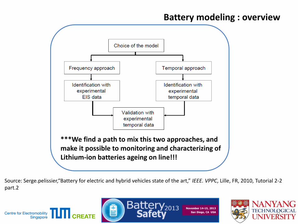
Battery modeling : overview

22

Source: Serge.pelissier,“Battery for electric and hybrid vehicles state of the art,” IEEE. VPPC, Lille, FR, 2010, Tutorial 2-2 part.2

***We find a path to mix this two approaches, and make it possible to monitoring and characterizing of Lithium-ion batteries ageing on line!!!

Experiment: Effect of Discharging Current

23

• We conduct experiments with discharging current of 1C, 1.5C and 2C to examine the impact of the discharging current on the model parameters. The results are shown in Table 5

Discharging

Current

𝑹𝟏 𝛀 𝑹𝟏𝑪𝒘 𝒔 𝒌 𝛀 𝑸𝒎 𝑪 𝒎𝟏 𝒎𝟐 rmse(V) Accuracy

2C 0.140 1360.65 0.000874 2.13 1 0.5 0.0144 0.996

1.5C 0.159 1533.19 0.000108 2.18 1 0.5 0.0148 0.996

1C 0.175 2045.91 0.000176 2.17 1 0.5 0.0153 0.996

Table 5 Model Parameters determined from discharging curves at different discharging currents

• Larger discharging current => the diffusion of the ionic species to move faster in the electrolyte => Warburg element will be smaller as show in Table 5

• Larger discharging current => too many charges arriving at the negative electrode per unit time => render inefficient storage of charges=> apparent Qm smaller

Experiment: Effect of Changing Discharging Current

24

• Since discharging current affect the model parameters, we use the values in Table 5 to determine the discharge curve of our battery cell with step change in the discharging current, with 30 minutes in between the step change.

Fig.10. Comparison of our computed and experimental discharging curve

***The maximum error in the battery voltage is 0.0808V and the root mean square error in the battery voltage is only 0.0326V, which is very small. The larger deviation occur at lower battery voltage (or correspondingly lower SoC) is due possibly to the fact that our model assumption is for SoC>50%!

0 10 20 30 40 50 60

3.0

3.2

3.4

3.6

3.8

4.0

4.2

Te

rmin

al V

olta

ge

(V

)

Discharging time (mins)

Experiment

Simulation

1C

1.5C

2C

Application of the Battery Model

25

• This method is fast and accurate, taking approximately 0.3011s , and can easily be implemented in most practical applications.

Fig.11. An implementation flow-chart of SoC estimation

“A Practical Framework of electrical based On-line SoC Estimation of Lithium-Ion Battery”, Journal of power source, F Leng, CM, Tan, R Yazami, MD, Le (under review)

Model : Limitation

26

As this is a first attempt to relate the electrochemical process in Li-Ion battery to the components in electrical , we limit our study to the following situation: • The self-discharge behavior of the battery is not considered. This can be

considered only if the physical-chemistry process of the self-discharge is well understood.

• The temperature of the battery during discharging is assumed to be constant. The model in this work can in principle be extended to include the temperature effect by making the components in the equivalent circuit to be temperature dependent. This will be considered in our future work with experimental data.

• SoC is always above 50% for practical consideration. Extension to SoC all the way to 20% will be considered in future.

• No high discharging current so that Peukert effect is insignificant.

Characterization of battery Aging

27

Aging = irreversible damage to battery , and hence loss of performances

28

Aging Introduction:

Storage aging (Calendar aging)

Cycling aging

SoC Temperature SoC Temperature

DoD

Current profile Discharging C-rate

Cycling aging depend very much on the application (Portable device, EV, HEV.etc)

29

Lithium-ion battery main ageing mechanisms: Cause Electrolyte

decomposition

(SEI formation)

Solvent co-intercalation,

gas evolution and

subsequent cracking

formation in particles

Decrease of accessible

surface area due to

continuous SEI growth

Changes in porosity

due to volume

changes, SEI formation

and growth

Contact loss of

active material

particles due to

volume changes

during cycling

Effect • Loss of lithium

• impedance rise

• Loss of active

material (graphite

exfoliation)

• Loss of lithium

• Impedance rise • Impedance rise • Loss of active

material

• J. Vetter, M. Winter, M. Wohlfahrt-Mehrens “ageing mechanisms in Lithium-ion batteries”, J.Electrochem. Soc, Vol.154, No.8, pp.393-403, 2009

Our Cycling Test: • The charging process is carried out at a fixed charging rate

of 0.7C in CC mode and a voltage of 4.2V in CV mode with a charge-termination current of 110mA, according to the company specification. Since this work focus only on the discharging process, the charging condition is fixed for all cases.

• Cycling the battery under constant ambient temperature and fixed constant discharging C-rate (1C, 1.5C and 2C) to the cut-off voltage of 3V as shown in the battery specification

30

Design of aging tests:

31

Electrode/Electrolyte Interface degradation

Source: Samartha A. Channagiri, Shrikant C. Nagpure, S.S. Babu, Garret J. Noble, Richard T. Hart “Porosity and phase fraction evolution with aging in lithium ion phosphate batter cathode”J.Power Sources, vol.243 ,pp.750–757, 2013.

32

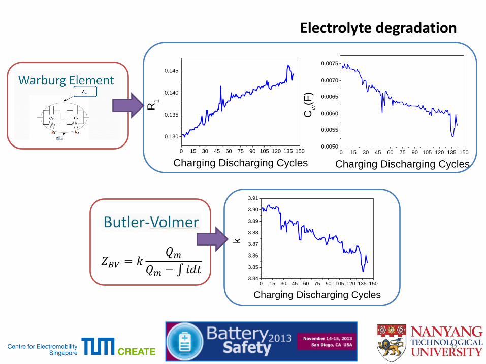
Electrolyte degradation

0 15 30 45 60 75 90 105 120 135 150

0.130

0.135

0.140

0.145

R1

Charging Discharging Cycles

0 15 30 45 60 75 90 105 120 135 1500.0050

0.0055

0.0060

0.0065

0.0070

0.0075

Cw(F

)

Charging Discharging Cycles

𝑍𝐵𝑉 = 𝑘𝑄𝑚

𝑄𝑚 − 𝑖𝑑𝑡

0 15 30 45 60 75 90 105 120 135 1503.84

3.85

3.86

3.87

3.88

3.89

3.90

3.91

k

Charging Discharging Cycles

𝑸𝒎𝒂𝒙+ = 𝒎𝟏𝑸𝒎 ,𝒎𝟏 ≤ 𝟏 ,

𝑸𝒎𝒂𝒙− = 𝒎𝟐𝑸𝒎 ,𝒎𝟐 ≤

𝟏

𝟐 ;

33

Electrode degradation

0 20 40 60 80 100 1200.90

0.92

0.94

0.96

0.98

1.00

1.02

1.04

1.06

1.08

1.10

m1

number of cycles

m1

0 20 40 60 80 100 1200.45

0.46

0.47

0.48

0.49

0.50

0.51

0.52

m2

number of cycles

m2

34

The rate of change of different model parameters that correspond to different ageing mechanisms

0

2

4

6

8

10

12

14

16

18

20

Re+Rct R1 Cw k m1 m2

% V

aria

tio

n o

f m

od

el p

aram

ete

rs

35

In-situ time domain characterization method

Temperature

DoD

Constant discharging Discharging C-rate

Current Profile Application

Different test conditions (Factors of ageing) Different ageing characteristics

Discharging curve

+

Proposed battery model

36

Conclusion

• An electrical model is developed in this work, and it can

determine 𝑄𝑚 easily after every discharge cycle, making the

estimation of SoH and SoC using Coulomb counting

method more accurate.

• This electrical model is able to provide an in-situ time-

domain characterization method that enables us to monitor

the different aging mechanisms under various operating

conditions on-line through its discharge curve alone, and

identify the dominant degradation mechanisms.

• The rate of aging through SoH determination allows

estimation of the Remain Useful Lifetime (RUL).

37

Thank you

Q & A