Only for Reading

Do not Download

Contents lists available at ScienceDirect

Scientia Horticulturae

journal homepage: www.elsevier.com/locate/scihorti

Real-time irrigation: Cost-effectiveness and benefits for water use andproductivity of strawberries

Laurence Gendrona,⁎,1, Guillaume Létourneaua, Lelia Andersona, Guillaume Sauvageaua,Claire Depardieua, Emily Paddockb, Allison van den Houtb, Raymond Levalloisc,Oleg Daugovishd, Samuel Sandoval Solise, Jean Carona,⁎

a Soil Science and Agri-Food Engineering Department, Pavillon de l'Envirotron, Université Laval, 2480, boulevard Hochelaga, Quebec (Qc), G1V 0A6, CanadabDriscoll’s, 1750 San Juan Rd, Aromas, CA, 95004, United Statesc Department of Agricultural Economics and Consumer Science, Pavillon Paul-Comtois, Université Laval, 2425, rue de l’Agriculture, Quebec (Qc), G1V 0A6, Canadad Division of Agriculture and Natural Resources, University of California Cooperative Extension, 669 County Square Drive, #100, Ventura, CA, 93003, United Statese Department of Land, Air and Water Resources, University of California, Veihmeyer Hall #135, 393, N Quad, Davis, CA, 95616, United States

A R T I C L E I N F O

Keywords:Tension sensorsSoil matric potentialConventional practiceWater use efficiencyEconomic analysisPrecision irrigation

A B S T R A C T

Although California is experiencing permanent water deficits compensated by irrigation, the state accounts formore than 90% of total strawberry production in the United States. There is a critical need to optimize yield andcrop water productivity (CWP), as influenced by irrigation management. Although studies have reported thatirrigation management based on soil matric potential (ѱ) has the potential to increase yield and CWP comparedto conventional practices, the cost of this technology may be a limiting factor for some growers. In this study, weassessed the cost-effectiveness of wireless tensiometer technology (WTT) for field-grown strawberries inCalifornia in comparison with the conventional irrigation management. As a second step, we evaluated the cost-effectiveness of deficit irrigation. Using data from eight sites, we calculated multiple linear regressions (MLR) todescribe the relationship between: (1) fresh market yield and average soil matric potential reached before ir-rigation initiation (ѱirr) and (2) water use and ѱirr. Based on MLR results, we evaluated the technical perfor-mance of each irrigation management method and conducted an economic analysis. Our results showed thatadopting a precise irrigation scheduling tool such as WTT is cost-effective and leads to water savings relative toconventional irrigation. Our results also revealed that any water savings associated with a deficit irrigationstrategy are costly for strawberry growers.

1. Introduction

With more than 1.3 million metric tonnes of strawberries (Fragaria xananassa Duch.) produced each year, the United States is the world’ssecond largest supplier for both fresh and frozen markets (FAOSTAT,2016). Remarkably, California leads all states in strawberry production,accounting for more than 90% of U.S. production (U.S. Department ofAgriculture, 2013). Because of sustained and severe drought conditions,the major strawberry growing regions of California experienced sub-stantial water supply problems between 2011–16 (USDA, 2016). Thestate relies heavily on irrigation, with much of the surface irrigationwater supplied by state and federal water projects (USDA, 2016). In

drought years, however, many farmers compensate for reduced surfacewater delivery by increasing water withdrawals from groundwaterwells (USDA, 2016). In addition, certain areas of coastal California donot have access to the delivered irrigation water and therefore relysolely on well water. The western United States is currently facing anumber of difficulties, including long-term aquifer depletion, potentialland subsidence, and salt water intrusion and nitrate contamination inlocal aquifers (California Departement of Water Resources, 2014;Fulcher et al., 2016; Gallardo et al., 1996; Gray et al., 2015; Scanlonet al., 2012). This situation can be particularly critical when aquifersare non-renewable sources of freshwater with naturally low rechargerates, which is found in many areas (USDA, 2016). Consequently, there

https://doi.org/10.1016/j.scienta.2018.06.013Received 3 March 2018; Received in revised form 22 May 2018; Accepted 6 June 2018

⁎ Corresponding authors.

1 Present address: Direction régionale de la Mauricie, Ministère de l’Agriculture, des Pêcheries et de l’Alimentation du Québec, 5195, boulevard des Forges, Trois-Rivières (QC), GY84Z3.

E-mail addresses: laurence.gendron.1@ulaval.ca (L. Gendron), jean.Caron@fsaa.ulaval.ca (J. Caron).

Abbreviations: ѱirr, soil matric potential at irrigation initiation; IT, irrigation threshold; WTT, wireless tensiometer technology; CWP, crop water productivity; RCBD, randomizedcomplete block design; MLR, multiple linear regression; FMY, fresh market yields; WU, water use; BEP, break-even point; EV, expected value; DI, deficit irrigation

Scientia Horticulturae 240 (2018) 468–477

0304-4238/ © 2018 Elsevier B.V. All rights reserved.

T

Only for Reading

Do not Download

is a critical need to increase crop water productivity to ensure rationalfreshwater use in areas of intensive agricultural activity (Lea-Cox et al.,2013).

Strawberry plants are sensitive to water stress (Hanson, 1931) dueto their shallow root system (Manitoba Minister of Agriculture, Foodand Rural Development, 2015). When the crop is drip irrigated, ade-quate irrigation management is required to meet plant water require-ments because only limited volumes of soil are wetted (Coelho and Or,1998). The effectiveness of such irrigation is highly dependent on itsscheduling, and it is thus important to determine the best timing andduration of irrigation events to limit over-watering, which often resultsin wasted water and soluble nutrients and lower crop yields (Saleemet al., 2013; Létourneau et al., 2015). Irrigation management practiceshave been studied extensively in field-grown strawberries (El-Farhanand Pritts, 1997). The methods most commonly used in California arebased either on crop evapotranspiration (ET) or on soil moisture mea-surements.

Evapotranspiration estimates the quantity of water used by the cropduring a given time period based on weather data and a field estimateof crop coefficients (Kc) (Grattan et al., 1998). Several studies havereported that ET-based irrigation has the potential to optimize waterapplications in strawberries (Cahn et al., 2016; Hanson and Bendixen,2004; Yuan et al., 2004). Despite being an inexpensive decision-makingtool (costs are negligible as many websites offer free access to potentialevapotranspiration calculations and tabulated crop coefficient values;Allen et al., 1998; California Irrigation Management InformationSystem, 2017), this approach estimates water usage indirectly andtherefore is not as accurate as direct-measurement methods (Lea-Cox,2012). To compensate for crop evapotranspiration losses (Allen et al.,1998), ET estimates past water requirements to predict future waterapplications, thus eliminating the possibility of managing irrigation inreal-time. While common grower practices aim for water applicationsequivalent to approximately 100% of crop ET, recent studies suggestthat improved irrigation scheduling methods, such as irrigation basedon soil matric potential (ѱ), can generate water savings without com-promising strawberry yields or fruit quality, once an optimal irrigationthreshold (IT) has been defined (Muñoz-Carpena et al., 2003;Létourneau et al., 2015; Migliaccio et al., 2008; Shae et al., 1999). Byoptimizing irrigation efficiency, the ѱ-based method is likely to enablestrawberry farmers to better meet sustainability and economic objec-tives.

Wireless soil sensor technology combines traditional soil matricpotential monitoring with wireless communication, thus allowing real-time data reporting and irrigation management (Chappell et al., 2013;Lea-Cox et al., 2013). In California, it has been shown that yields de-creased sharply at soil matric potentials of less than −8 to −12 kPa insandy loam to clay loam soils, suggesting that ѱ-based irrigation mayprovide optimal yield and CWP at soil matric potentials ranging from−10 to −15 kPa in field-grown strawberries (Létourneau et al., 2015).In similar conditions, Anderson (2015) showed that ѱ-based irrigationat an IT of −17 kPa could increase yield and CWP compared to con-ventional irrigation which was usually drier (ѱirrs of −27, −31 and−42 kPa). These results are consistent with other research studies,where significantly higher strawberry yields were obtained using an ITof −10 kPa compared to ITs ranging from −30 to −70 kPa (Guimeràet al., 1995; Peñuelas et al., 1992; Serrano et al., 1992). Although mostgrowers are receptive to the idea of wireless sensor networks, they haveso far been reluctant to adopt WTT because it is more costly – involvingan investment in equipment of more than $1500 per hectare – than theconventional irrigation management method (Majsztrik et al., 2013;Lea-Cox, 2012). However, no analysis assessing the cost-effectiveness ofthis technology has been conducted for strawberry production in NorthAmerica.

WTT also opens up a range of possibilities for fine-tuned irrigationstrategies, such as deficit irrigation (DI), which has been shown to re-duce water use and improve CWP in many crops (Geerts and Raes,

2009; Fereres and Soriano, 2007; Zwart and Bastiaanssen, 2004). Instrawberries, Létourneau et al. (2015) obtained higher CWP in driertreatments (lower ITs) than in wetter treatments (−26 kPa vs −10 kPa;−15 kPa vs −8 kPa). Likewise, in Finland, in a strawberry crop grownin a sandy soil, Hoppula and Salo (2007) obtained higher CWP withirrigation initiated at −60 kPa instead of −15 kPa. Considering thatmost Californian strawberry growers must pay for water, it could bebeneficial to develop a controlled dry-irrigation management strategythat uses tension sensors to save water.

In this study, we first assessed the cost-effectiveness of ѱ-basedmanagement using WTT with an optimal IT of −10 kPa in field-grownstrawberries in California, in comparison with the conventional irri-gation management method. In a second time, we evaluated the cost-effectiveness of deficit irrigation using WTT by simulating a set of re-duced-irrigation scenarios.

2. Materials and methods

2.1. Site description and experimental designs

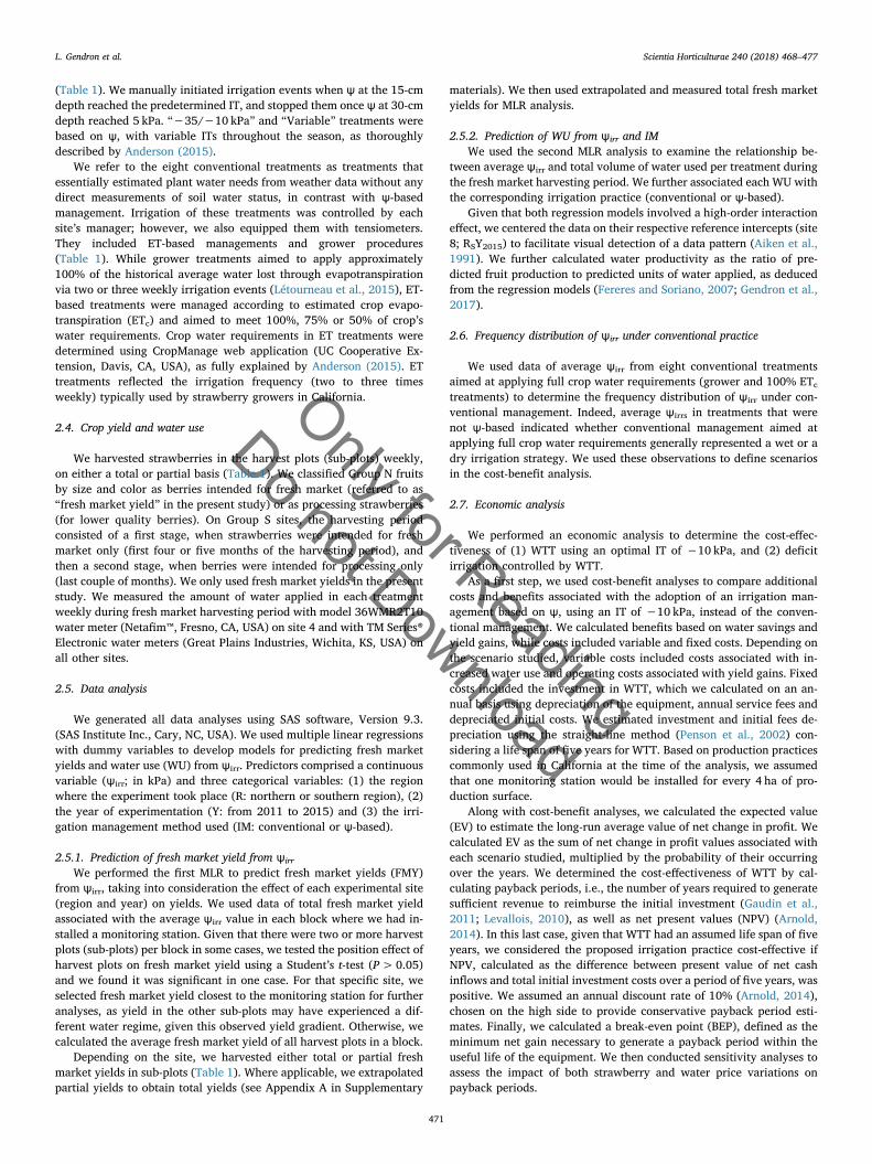
We collected the data analyzed in this study over five growingseasons and on eight experimental sites covering a range of soil prop-erties, cultivation periods, strawberry cultivars and farming practicesused in field strawberry production in California, USA (Table 1). Wearranged treatments in all sites except site 1 in a randomized completeblock design (RCBD) with three to five replicates (Table 1). We dividedsites, all located in a typical temperate, Mediterranean climate, into twogroups according to their location: northern strawberry growing region(Group N: sites 1–4) and southern strawberry growing region (Group S:sites 5–8). We grew strawberry plants on raised beds covered with aplastic mulch according to standard farming practices (Strand, 2008),with two (Group N) or four (Group S) plant rows per bed. In Group N,day-neutral strawberries (Fragaria× ananassa Duch.) were planted bythe farm team in November in silty clay and clay loam soils. Trials ranfrom April to October on sites 1, 3 and 4, and from mid-April to lateJune on site 2. In Group S, short-day strawberries were planted by thefarm team in sandy loam soils in October with fresh market harvestperiod falling between January/February and May/June, depending onthe growing season.

2.2. Irrigation system specifications and ѱirr measurements

At all sites, sprinkler irrigation was used by the farm team up toproper establishment (for 4–6 weeks after planting). Subsequently, weused drip-irrigation until the end of the season. We irrigated growingbeds by two (Group N) or three (Group S) drip lines (0.34–0.70 L·h−1

per emitter, depending on the site, with 20-cm emitter spacing). Weinstalled field monitoring stations reporting real-time ѱ measurementsthrough wireless networks and web servers in all treatments in one ortwo blocks (Group N) or in one to three blocks (Group S) (Table 1). ATX3 wireless monitoring station (Hortau, Quebec, Qc, Canada) con-sisted of two model HXM80 tensiometers, buried at two different depths(15 and 30 cm), that measured ѱ at 15-min intervals. In ѱ-basedtreatments, the shallow probe, located in the root zone, indicated whena set IT was reached and when irrigation should be initiated. The deepprobe, located below the root zone, indicated when to stop irrigation toprevent water percolation and nutrient leaching under the root zone. Inconventional treatments, the probe at a 15-cm depth reported theaverage soil matric potential reached before irrigation and the deepprobe monitored the soil water status at a 30-cm depth.

2.3. Irrigation treatments

Irrigation treatments in our study concern post-establishment irri-gation. A total of twenty-five ѱ-based treatments consisted of differentirrigation initiation thresholds ranging from −8 kPa to −35 kPa

L. Gendron et al. Scientia Horticulturae 240 (2018) 468–477

469

Only for Reading

Do not Download

Table1

Site

descriptionan

dirriga

tion

treatm

ents.

Group

Site

Location

(lat;lon

g)Year

Freshmarke

tha

rvestpe

riod

Soil

type

Site

area

(ha)

Bedleng

th/

width

(m)

Num

berof

beds

perplot

Expe

rimen

tal

design

Num

berof

harvestplots

(sub

-plots)

Num

berof

mon

itoring

stations/trtb

Harve

stfreq

uenc

y(P

cor

Td)

Treatm

ents

(irrigationman

agem

ent)

Con

ventiona

leѱ-based

(VWCf )

N1

Watsonv

ille,

CA,

USA

(368

8°;-12

1,81

°)

2011

Aprilto

Octob

erSilty

clay

0.28

55/0

.80

14Notreatm

ent

replicate

31

PGrower

−10

kPa(0.60)

−20

kPa(0.55)

N2

Salin

as,C

A,

USA

(366

9°;-12

1,65

°)

2012

Mid-Aprilto

late

June

Siltyclay

loam

0.56

127/

0.80

4RCBD

a

3reps

21

PNA

−8kP

a(0.45)

−13

kPa(0.44)

−18

kPa(0.42)

N3

Watsonv

ille,

CA,

USA

(368

9°;-12

2,67

°)

2013

Aprilto

Octob

erClay

loam

0.28

32/0

.80

2RCBD

4reps

11

TGrower

−10

kPa(0.60)

−17

kPa(0.57)

−25

kPa(0.53)

N4

Watsonv

ille,

CA,

USA

(368

9°;-12

1,67

°)

2014

Aprilto

Octob

erClay

loam

0.19

34/0

.80

1RCBD

4reps

22

P50

%ET

c75

%ET

c10

0%ET

cGrower

−10

kPa(0.60)

−35

kPa/−

10kP

a(0.50/

0.60

)

S5

Oxn

ard,

CA,

USA

(34.15

°,-119

.15°)

2012

Februa

ryto

mid-

June

Sand

yloam

0.70

130/

1.22

3RCBD

3reps

21

TNA

−8kP

a(0.36)

−11

kPa(0.35)

−13

kPa(0.34)

S6

Oxn

ard,

CA,

USA

(341

9°;-11

9,19

°)

2013

Janu

aryto

May

Sand

yloam

NA

NA

2RCBD

3reps

21

PGrower

−13

kPa(0.34)

−13

kPa(0.34)

−18

kPa(0.33)

S7

Oxn

ard,

CA,

USA

(341

9°;-11

9,19

°)

2014

Janu

aryto

June

Sand

yloam

0.55

127/

1.22

1RCBD

5reps

23

PGrower

−10

kPa(0.35)

−35

kPa(0.30)

−35

kPa/-10kP

a(0.30/

0.35

)Variablethresholds

S8

Oxn

ard,

CA,

USA

(341

9°;-11

9,19

°)

2015

Janu

aryto

June

Sand

yloam

0.55

119/

1.22

1RCBD

5reps

23

PNA

−10

kPa(0.35)

−35

kPa(0.30)

−35

kPa/-10kP

a(0.30/

0.35

)Variablethresholds

Grower

(ѱ-based

)g

a RCBD

:Ran

domized

Com

pleteBloc

kDesign.

bSo

mesitesha

dreplicates

withon

esensor

perexpe

rimen

talun

itan

ddidthereforeha

veman

ysensorspe

rtreatm

ents.Onothe

rsites,

whe

rewewereim

posedlim

itationof

equipm

ent,therewas

onetensiometer

per

treatm

ent.In

thesecases,co

resamples

(sitech

aracterization

)weretake

nat

thebe

ginn

ingof

theexpe

rimen

ttoch

ecktheun

iformity.

Also,

earlymeasuremen

tsweretake

nwithtensiometersat

multiplelocation

sto

mak

esure

that

thesite

chosen

was

represen

tative

oftheva

riab

ility.

c P(partial

yield):whe

nha

rvestby

theresearch

team

was

done

less

oftenthan

that

ofthegrow

er.

dT(total

yield):w

henha

rvestby

theresearch

team

was

done

asoftenas

that

ofthegrow

er.

e Con

ventiona

ltreatmen

tswereessentially

estimated

from

weather

data

witho

utan

ydirect

measuremen

tof

soilwater

status,inco

ntrast

withѱ-based

treatm

ents,a

ndwereirriga

tedat

thesamefreq

uenc

y(twoto

three

times

weekly).

f VWC:v

olum

etricwater

conten

t.Th

ispa

rameter

was

notm

easuredon

sitesan

dwas

rather

estimated

from

publishe

dwater

desorption

curves

from

thesamesites(A

nderson,

2015

).Asthewater

conten

t-matricpo

tential

relation

ship

depe

ndson

soiltexture,

soilstuc

ture

andhy

sterisis

phen

omen

a,thesite

water

conten

tva

lueev

enwithinasamesite

isap

prox

imateon

ly.R

eading

swithVWCprob

esalso

need

slocalcalib

ration

formore

accu

rate

estimate.

Localcalib

ration

ofVWCwithtensim

eter

read

ings

isthereforereco

mmen

dedto

establishco

rrespo

ndan

cewiththesoilwater

potentialva

lues

impo

sedin

theseexpe

rimen

ts.

g The

grow

ertreatm

enton

site

8was

includ

edin

theѱ-based

treatm

ents

sinc

ewirelesstensiometer

tech

nology

was

used

toman

ageirriga

tion

.

L. Gendron et al. Scientia Horticulturae 240 (2018) 468–477

470

Only for Reading

Do not Download

(Table 1). We manually initiated irrigation events when ѱ at the 15-cmdepth reached the predetermined IT, and stopped them once ѱ at 30-cmdepth reached 5 kPa. “−35/−10 kPa” and “Variable” treatments werebased on ѱ, with variable ITs throughout the season, as thoroughlydescribed by Anderson (2015).

We refer to the eight conventional treatments as treatments thatessentially estimated plant water needs from weather data without anydirect measurements of soil water status, in contrast with ѱ-basedmanagement. Irrigation of these treatments was controlled by eachsite’s manager; however, we also equipped them with tensiometers.They included ET-based managements and grower procedures(Table 1). While grower treatments aimed to apply approximately100% of the historical average water lost through evapotranspirationvia two or three weekly irrigation events (Létourneau et al., 2015), ET-based treatments were managed according to estimated crop evapo-transpiration (ETc) and aimed to meet 100%, 75% or 50% of crop’swater requirements. Crop water requirements in ET treatments weredetermined using CropManage web application (UC Cooperative Ex-tension, Davis, CA, USA), as fully explained by Anderson (2015). ETtreatments reflected the irrigation frequency (two to three timesweekly) typically used by strawberry growers in California.

2.4. Crop yield and water use

We harvested strawberries in the harvest plots (sub-plots) weekly,on either a total or partial basis (Table 1). We classified Group N fruitsby size and color as berries intended for fresh market (referred to as“fresh market yield” in the present study) or as processing strawberries(for lower quality berries). On Group S sites, the harvesting periodconsisted of a first stage, when strawberries were intended for freshmarket only (first four or five months of the harvesting period), andthen a second stage, when berries were intended for processing only(last couple of months). We only used fresh market yields in the presentstudy. We measured the amount of water applied in each treatmentweekly during fresh market harvesting period with model 36WMR2T10water meter (Netafim™, Fresno, CA, USA) on site 4 and with TM Series®Electronic water meters (Great Plains Industries, Wichita, KS, USA) onall other sites.

2.5. Data analysis

We generated all data analyses using SAS software, Version 9.3.(SAS Institute Inc., Cary, NC, USA). We used multiple linear regressionswith dummy variables to develop models for predicting fresh marketyields and water use (WU) from ѱirr. Predictors comprised a continuousvariable (ѱirr; in kPa) and three categorical variables: (1) the regionwhere the experiment took place (R: northern or southern region), (2)the year of experimentation (Y: from 2011 to 2015) and (3) the irri-gation management method used (IM: conventional or ѱ-based).

2.5.1. Prediction of fresh market yield from ѱirr

We performed the first MLR to predict fresh market yields (FMY)from ѱirr, taking into consideration the effect of each experimental site(region and year) on yields. We used data of total fresh market yieldassociated with the average ѱirr value in each block where we had in-stalled a monitoring station. Given that there were two or more harvestplots (sub-plots) per block in some cases, we tested the position effect ofharvest plots on fresh market yield using a Student’s t-test (P>0.05)and we found it was significant in one case. For that specific site, weselected fresh market yield closest to the monitoring station for furtheranalyses, as yield in the other sub-plots may have experienced a dif-ferent water regime, given this observed yield gradient. Otherwise, wecalculated the average fresh market yield of all harvest plots in a block.

Depending on the site, we harvested either total or partial freshmarket yields in sub-plots (Table 1). Where applicable, we extrapolatedpartial yields to obtain total yields (see Appendix A in Supplementary

materials). We then used extrapolated and measured total fresh marketyields for MLR analysis.

2.5.2. Prediction of WU from ѱirr and IMWe used the second MLR analysis to examine the relationship be-

tween average ѱirr and total volume of water used per treatment duringthe fresh market harvesting period. We further associated each WU withthe corresponding irrigation practice (conventional or ѱ-based).

Given that both regression models involved a high-order interactioneffect, we centered the data on their respective reference intercepts (site8; RSY2015) to facilitate visual detection of a data pattern (Aiken et al.,1991). We further calculated water productivity as the ratio of pre-dicted fruit production to predicted units of water applied, as deducedfrom the regression models (Fereres and Soriano, 2007; Gendron et al.,2017).

2.6. Frequency distribution of ѱirr under conventional practice

We used data of average ѱirr from eight conventional treatmentsaimed at applying full crop water requirements (grower and 100% ETc

treatments) to determine the frequency distribution of ѱirr under con-ventional management. Indeed, average ѱirrs in treatments that werenot ѱ-based indicated whether conventional management aimed atapplying full crop water requirements generally represented a wet or adry irrigation strategy. We used these observations to define scenariosin the cost-benefit analysis.

2.7. Economic analysis

We performed an economic analysis to determine the cost-effec-tiveness of (1) WTT using an optimal IT of −10 kPa, and (2) deficitirrigation controlled by WTT.

As a first step, we used cost-benefit analyses to compare additionalcosts and benefits associated with the adoption of an irrigation man-agement based on ѱ, using an IT of −10 kPa, instead of the conven-tional management. We calculated benefits based on water savings andyield gains, while costs included variable and fixed costs. Depending onthe scenario studied, variable costs included costs associated with in-creased water use and operating costs associated with yield gains. Fixedcosts included the investment in WTT, which we calculated on an an-nual basis using depreciation of the equipment, annual service fees anddepreciated initial costs. We estimated investment and initial fees de-preciation using the straight-line method (Penson et al., 2002) con-sidering a life span of five years for WTT. Based on production practicescommonly used in California at the time of the analysis, we assumedthat one monitoring station would be installed for every 4 ha of pro-duction surface.

Along with cost-benefit analyses, we calculated the expected value(EV) to estimate the long-run average value of net change in profit. Wecalculated EV as the sum of net change in profit values associated witheach scenario studied, multiplied by the probability of their occurringover the years. We determined the cost-effectiveness of WTT by cal-culating payback periods, i.e., the number of years required to generatesufficient revenue to reimburse the initial investment (Gaudin et al.,2011; Levallois, 2010), as well as net present values (NPV) (Arnold,2014). In this last case, given that WTT had an assumed life span of fiveyears, we considered the proposed irrigation practice cost-effective ifNPV, calculated as the difference between present value of net cashinflows and total initial investment costs over a period of five years, waspositive. We assumed an annual discount rate of 10% (Arnold, 2014),chosen on the high side to provide conservative payback period esti-mates. Finally, we calculated a break-even point (BEP), defined as theminimum net gain necessary to generate a payback period within theuseful life of the equipment. We then conducted sensitivity analyses toassess the impact of both strawberry and water price variations onpayback periods.

L. Gendron et al. Scientia Horticulturae 240 (2018) 468–477

471

Only for Reading

Do not Download

As a second step, we conducted cost-benefit analyses to assess thecost-effectiveness of deficit irrigation controlled by WTT. Analyses ac-counted for variations in yield and water use when DI strategies wereadopted instead of the optimal IT of −10 kPa. We conducted sensitivityanalyses to assess the impact of water price variations on cost-effec-tiveness of deficit irrigation.

We conducted cost-benefit analyses on a one-hectare basis, sincefarm size had a negligible impact on net changes in profit (data notshown). We predicted FMY and WU values from the fitted regressionmodels. We reported input costs and output prices as in Appendix B (inSupplementary materials).

3. Results

3.1. Multiple linear regressions

3.1.1. Prediction of fresh market yield from ѱirr

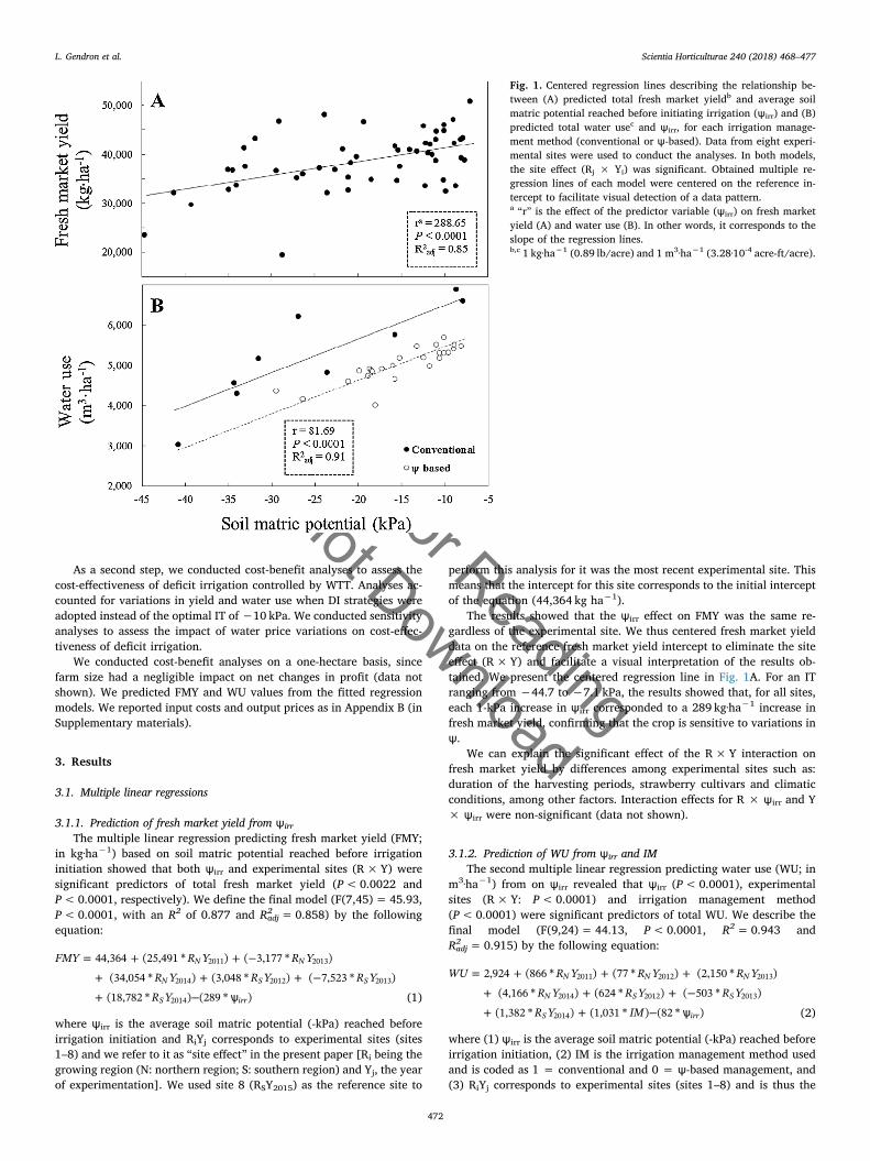
The multiple linear regression predicting fresh market yield (FMY;in kg·ha−1) based on soil matric potential reached before irrigationinitiation showed that both ѱirr and experimental sites (R×Y) weresignificant predictors of total fresh market yield (P<0.0022 andP<0.0001, respectively). We define the final model (F(7,45)= 45.93,P<0.0001, with an R2 of 0.877 and R2

adj=0.858) by the followingequation:

ѱ

= + + −

+ + + −

+ −

FMY R Y R Y

R Y R Y R Y

R Y

44,364 (25,491 * ) ( 3,177 * )

(34,054 * ) (3,048 * ) ( 7,523 * )

(18,782 * ) (289 * )

N N

N S S

S irr

2011 2013

2014 2012 2013

2014 (1)

where ѱirr is the average soil matric potential (-kPa) reached beforeirrigation initiation and RiYj corresponds to experimental sites (sites1–8) and we refer to it as “site effect” in the present paper [Ri being thegrowing region (N: northern region; S: southern region) and Yj, the yearof experimentation]. We used site 8 (RSY2015) as the reference site to

perform this analysis for it was the most recent experimental site. Thismeans that the intercept for this site corresponds to the initial interceptof the equation (44,364 kg ha−1).

The results showed that the ѱirr effect on FMY was the same re-gardless of the experimental site. We thus centered fresh market yielddata on the reference fresh market yield intercept to eliminate the siteeffect (R×Y) and facilitate a visual interpretation of the results ob-tained. We present the centered regression line in Fig. 1A. For an ITranging from −44.7 to −7.1 kPa, the results showed that, for all sites,each 1-kPa increase in ѱirr corresponded to a 289 kg·ha−1 increase infresh market yield, confirming that the crop is sensitive to variations inѱ.

We can explain the significant effect of the R×Y interaction onfresh market yield by differences among experimental sites such as:duration of the harvesting periods, strawberry cultivars and climaticconditions, among other factors. Interaction effects for R × ѱirr and Y× ѱirr were non-significant (data not shown).

3.1.2. Prediction of WU from ѱirr and IMThe second multiple linear regression predicting water use (WU; in

m3·ha−1) from on ѱirr revealed that ѱirr (P<0.0001), experimentalsites (R×Y: P<0.0001) and irrigation management method(P<0.0001) were significant predictors of total WU. We describe thefinal model (F(9,24)= 44.13, P<0.0001, R2=0.943 andR2adj=0.915) by the following equation:

ѱ

= + + +

+ + + −

+ + −

WU R Y R Y R Y

R Y R Y R Y

R Y IM

2,924 (866 * ) (77 * ) (2,150 * )

(4,166 * ) (624 * ) ( 503 * )

(1,382 * ) (1,031 * ) (82 * )

N N N

N S S

S irr

2011 2012 2013

2014 2012 2013

2014 (2)

where (1) ѱirr is the average soil matric potential (-kPa) reached beforeirrigation initiation, (2) IM is the irrigation management method usedand is coded as 1 = conventional and 0 = ѱ-based management, and(3) RiYj corresponds to experimental sites (sites 1–8) and is thus the

Fig. 1. Centered regression lines describing the relationship be-tween (A) predicted total fresh market yieldb and average soilmatric potential reached before initiating irrigation (ѱirr) and (B)predicted total water usec and ѱirr, for each irrigation manage-ment method (conventional or ѱ-based). Data from eight experi-mental sites were used to conduct the analyses. In both models,the site effect (Rj × Yi) was significant. Obtained multiple re-gression lines of each model were centered on the reference in-tercept to facilitate visual detection of a data pattern.a “r” is the effect of the predictor variable (ѱirr) on fresh marketyield (A) and water use (B). In other words, it corresponds to theslope of the regression lines.b,c 1 kg·ha−1 (0.89 lb/acre) and 1 m3·ha−1 (3.28·10-4 acre-ft/acre).

L. Gendron et al. Scientia Horticulturae 240 (2018) 468–477

472

Only for Reading

Do not Download

“site effect” [Ri being the growing region (N: northern region; S:southern region) and Yj, the year of experimentation]. We again usedsite 8 (RSY2015) as the reference site to perform this analysis for it wasthe most recent experimental site. This means that the intercept for thissite corresponds to the initial intercept of the equation (2924).

Since the effect of ѱirr on WU of each IM was the same regardless ofthe experimental site, we centered the WU data as described above andfurther increased by 3333 m3·ha−1 to obtain positive values of WU onthe entire range of ѱirr, thus facilitating visual detection of a datapattern. We show the centered regression line in Fig. 1B.

Considering ITs ranging from −40.8 to −7.9 kPa, we found a po-sitive relationship between water use and ѱirr, with a predicted WUincrease of 82 m3·ha−1 per kPa. Moreover, irrigation managementmethod had a significant effect on the amount of water applied. Indeed,the conventional management used constantly more water (1031m3·ha−1) than ѱ-based method (Fig. 1B). Hence, the results indicatethat we can expect an increase in CWP with the use of ѱ-based irri-gation management with WTT instead of conventional management(see Appendix C in Supplementary materials).

We can explain significant differences in WU between experimentalsites by inter-site variations such as: duration of the harvesting periods,climatic conditions, strawberry cultivars, soil types, among others.Interaction effect for Y × ѱirr, R × ѱirr, R× IM and Y× IM were notsignificant (data not shown).

3.2. Frequency distribution and studied scenarios

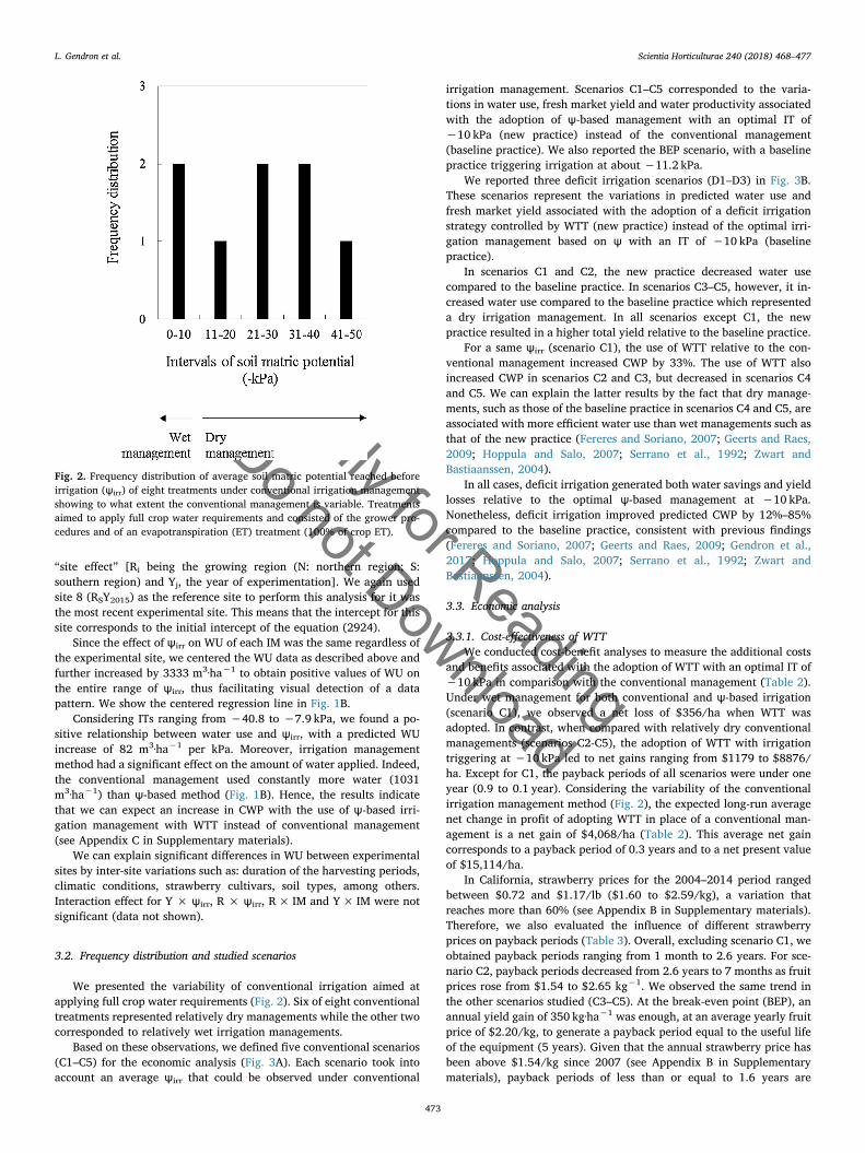
We presented the variability of conventional irrigation aimed atapplying full crop water requirements (Fig. 2). Six of eight conventionaltreatments represented relatively dry managements while the other twocorresponded to relatively wet irrigation managements.

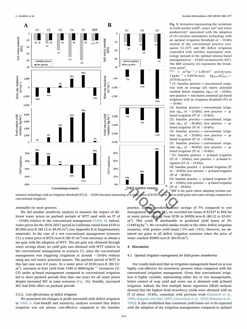
Based on these observations, we defined five conventional scenarios(C1–C5) for the economic analysis (Fig. 3A). Each scenario took intoaccount an average ѱirr that could be observed under conventional

irrigation management. Scenarios C1–C5 corresponded to the varia-tions in water use, fresh market yield and water productivity associatedwith the adoption of ѱ-based management with an optimal IT of−10 kPa (new practice) instead of the conventional management(baseline practice). We also reported the BEP scenario, with a baselinepractice triggering irrigation at about −11.2 kPa.

We reported three deficit irrigation scenarios (D1–D3) in Fig. 3B.These scenarios represent the variations in predicted water use andfresh market yield associated with the adoption of a deficit irrigationstrategy controlled by WTT (new practice) instead of the optimal irri-gation management based on ѱ with an IT of −10 kPa (baselinepractice).

In scenarios C1 and C2, the new practice decreased water usecompared to the baseline practice. In scenarios C3–C5, however, it in-creased water use compared to the baseline practice which representeda dry irrigation management. In all scenarios except C1, the newpractice resulted in a higher total yield relative to the baseline practice.

For a same ѱirr (scenario C1), the use of WTT relative to the con-ventional management increased CWP by 33%. The use of WTT alsoincreased CWP in scenarios C2 and C3, but decreased in scenarios C4and C5. We can explain the latter results by the fact that dry manage-ments, such as those of the baseline practice in scenarios C4 and C5, areassociated with more efficient water use than wet managements such asthat of the new practice (Fereres and Soriano, 2007; Geerts and Raes,2009; Hoppula and Salo, 2007; Serrano et al., 1992; Zwart andBastiaanssen, 2004).

In all cases, deficit irrigation generated both water savings and yieldlosses relative to the optimal ѱ-based management at −10 kPa.Nonetheless, deficit irrigation improved predicted CWP by 12%–85%compared to the baseline practice, consistent with previous findings(Fereres and Soriano, 2007; Geerts and Raes, 2009; Gendron et al.,2017; Hoppula and Salo, 2007; Serrano et al., 1992; Zwart andBastiaanssen, 2004).

3.3. Economic analysis

3.3.1. Cost-effectiveness of WTTWe conducted cost-benefit analyses to measure the additional costs

and benefits associated with the adoption of WTT with an optimal IT of−10 kPa in comparison with the conventional management (Table 2).Under wet management for both conventional and ѱ-based irrigation(scenario C1), we observed a net loss of $356/ha when WTT wasadopted. In contrast, when compared with relatively dry conventionalmanagements (scenarios C2-C5), the adoption of WTT with irrigationtriggering at −10 kPa led to net gains ranging from $1179 to $8876/ha. Except for C1, the payback periods of all scenarios were under oneyear (0.9 to 0.1 year). Considering the variability of the conventionalirrigation management method (Fig. 2), the expected long-run averagenet change in profit of adopting WTT in place of a conventional man-agement is a net gain of $4,068/ha (Table 2). This average net gaincorresponds to a payback period of 0.3 years and to a net present valueof $15,114/ha.

In California, strawberry prices for the 2004–2014 period rangedbetween $0.72 and $1.17/lb ($1.60 to $2.59/kg), a variation thatreaches more than 60% (see Appendix B in Supplementary materials).Therefore, we also evaluated the influence of different strawberryprices on payback periods (Table 3). Overall, excluding scenario C1, weobtained payback periods ranging from 1 month to 2.6 years. For sce-nario C2, payback periods decreased from 2.6 years to 7 months as fruitprices rose from $1.54 to $2.65 kg−1. We observed the same trend inthe other scenarios studied (C3–C5). At the break-even point (BEP), anannual yield gain of 350 kg·ha−1 was enough, at an average yearly fruitprice of $2.20/kg, to generate a payback period equal to the useful lifeof the equipment (5 years). Given that the annual strawberry price hasbeen above $1.54/kg since 2007 (see Appendix B in Supplementarymaterials), payback periods of less than or equal to 1.6 years are

Fig. 2. Frequency distribution of average soil matric potential reached beforeirrigation (ѱirr) of eight treatments under conventional irrigation managementshowing to what extent the conventional management is variable. Treatmentsaimed to apply full crop water requirements and consisted of the grower pro-cedures and of an evapotranspiration (ET) treatment (100% of crop ET).

L. Gendron et al. Scientia Horticulturae 240 (2018) 468–477

473

Only for Reading

Do not Downloadattainable for most growers.We did another sensitivity analysis to measure the impact of dif-

ferent water prices on payback periods of WTT used with an IT of−10 kPa relative to the conventional management (Table 4). Indeed,water prices for the 2016–2017 period in California varied from $150 to$5,000/acre-ft ($0.12 to $4.05/m3) (see Appendix B in Supplementarymaterials). In the case of a wet conventional management (scenarioC1), a water price of $575/acre-ft ($0.47/m3) was necessary to obtain anet gain with the adoption of WTT. The net gain was obtained throughwater savings alone; no yield gain was obtained with WTT relative tothe conventional management in scenario C1, since the conventionalmanagement was triggering irrigations at around −10 kPa withoutusing any soil matric potential sensors. The payback period of WTT inthis last case was 4.9 years. At a water price of $150/acre-ft ($0.12/m3), increases in fruit yield from 1440 to 8660 kg·ha−1 (scenarios C2-C5) under ѱ-based management compared to conventional irrigationled to short payback periods (less than one year) for all water pricesdespite increased WU in some scenarios (Fig. 3A). Notably, increasedWU had little effect on payback periods.

3.3.2. Cost-effectiveness of deficit irrigationWe presented net changes in profit associated with deficit irrigation

in Table 5. Cost-benefit and sensitivity analyses revealed that deficitirrigation was not always cost-effective compared to the baseline

practice. Despite predicted water savings of 7% compared to wetmanagement (scenario D1), we recorded net losses of $1537 to $92/haat water prices ranging from $150 to $4500/acre-ft ($0.12 to $3.65/m3). This result is attributable to predicted yield losses of 3%(1440 kg·ha-1). We revealed similar trends in the other deficit irrigationscenarios, with greater yield losses (-7% and -14%). However, we ob-tained net gains in all deficit irrigation scenarios when the price ofwater reached $5000/acre-ft ($4.05/m3).

4. Discussion

4.1. Optimal irrigation management for field-grown strawberries

Our results indicated that an irrigation management based on ѱ washighly cost-effective for strawberry growers when compared with theconventional irrigation management. Given that conventional irriga-tion is highly variable, representing either dry or wet managements,better control of crop yield and water use is obtained with ѱ-basedirrigation. Indeed, the first multiple linear regression (MLR) analysisshowed that the highest fresh strawberry yields were obtained with anIT of about -10 kPa, consistent with previous work (Guimerà et al.,1995; Hoppula and Salo, 2007; Létourneau et al., 2015; Peñuelas et al.,1992). It also established that consistent yield losses are to be expectedwith the adoption of dry irrigation managements compared to optimal

Fig. 3. Scenarios representing the variationsin fresh market yielda, water useb and waterproductivityc associated with the adoptionof (A) wireless tensiometer technology withan optimal irrigation threshold of −10 kPainstead of the conventional practice (sce-narios C1-C5d) and (B) deficit irrigationcontrolled with wireless tensiometer tech-nology instead of the optimal tension-basedmanagement at −10 kPa (scenarios D1-D3e).The BEP scenario (A) represents the break-even pointf.a,b,c 1 m3·ha−1 = 3.28·10-4 acre-ft/acre;1 kg·ha−1 = 0.89 lb/acre; kgfruit·m-3

water =2719 lb/acre-ft.d C1: baseline practice= conventional irriga-tion with an average soil matric potentialreached before irrigation (ѱirr) of −10 kPa;new practice= soil matric potential (ѱ)-basedirrigation with an irrigation threshold (IT) of−10 kPa.C2: baseline practice= conventional irriga-tion (ѱirr of −15 kPa); new practice = ѱ-based irrigation (IT of −10 kPa).C3: baseline practice= conventional irriga-tion (ѱirr of −25 kPa); new practice = ѱ-based irrigation (IT of −10 kPa).C4: baseline practice= conventional irriga-tion (ѱirr of −35 kPa); new practice = ѱ-based irrigation (IT of −10 kPa).C5: baseline practice= conventional irriga-tion (ѱirr of −40 kPa); new practice = ѱ-based irrigation (IT of −10 kPa).e D1: baseline practice = ѱ-based irrigation(IT of −10 kPa); new practice = ѱ-based ir-rigation (IT of −15 kPa).D2: baseline practice = ѱ-based irrigation (ITof−10 kPa); new practice = ѱ-based irrigation(IT of −20 kPa).D3: baseline practice = ѱ-based irrigation (ITof−10 kPa); new practice = ѱ-based irrigation(IT of −30 kPa).f BEP is the point where adopting wireless ten-

siometer technology with an irrigation threshold (IT) of−10 kPa becomes interesting at a water price of $150/acre-ft, due to yield gains and water savings compared toconventional irrigation.

L. Gendron et al. Scientia Horticulturae 240 (2018) 468–477

474

Only for Reading

Do not Download

management with an IT of −10 kPa. Interestingly, the analysis showedthat site-specific characteristics, such as region, climatic conditions, soiltypes, and strawberry cultivars, among others, did influence the totalamount of fresh fruits harvested at each site, but did not change theresponse of yield to the ѱirr. We can thus conclude that optimal irri-gation is attained with an IT of −10 kPa in open-field strawberryproduction in California.

In addition, the results of the second multiple linear regression in-dicated that conventional irrigation constantly used more water than ѱ-based irrigation to obtain a similar yield, regardless of the experimentalsite. Ѱ-based irrigation management thus appears to allow for moreefficient water use than the conventional management in open-fieldstrawberry production in California.

4.2. Adopting WTT: economic considerations

Our cost-benefit analyses showed that the cost-effectiveness of WTTwas highly dependent on yield. We calculated a payback period withinthe useful life of the equipment for a yield increase of only 350 kg·ha-1

with WTT. Likewise, given that the equipment is expected to last for 5years, we obtained short payback periods (under one year) for the in-vestment in WTT with high predicted yield gains (4330–8660 kg·ha−1)relative to conventional irrigation, even though these yield gains wereassociated with increased water use. This suggests that the current costof water is low since it has little influence on payback periods.Similarly, payback periods were relatively short (1.6–2.6 years) even atvery low strawberry prices, between $1.54 and $1.76/kg, suggestingthat the cost-effectiveness of the technology is not likely to be affectedby strawberry price variations.

In the case where the use of WTT instead of conventional irrigationgenerated only water savings, the current water price, ranging from$150 to $350/acre-ft ($0.12 to $0.28/m3) depending on the growingregion, was too low to generate a net gain for the grower. Indeed, aminimum water price of $575/acre-ft1 ($0.47/m3) would be required toensure the cost-effectiveness of WTT on the sole basis of water savings.This suggests that current water prices are not high enough to supportan investment in water-saving technologies, such as WTT.

However, regardless of water price, farmers can make better man-agement decisions with water allocations that they receive fromCalifornia groundwater pumping agencies (imposed during drought),while improved in-field monitoring would allow compliance with re-gional regulations on water use and discharge.

4.3. Deficit irrigation: unfortunately for the environment, an unprofitablestrategy so far

Our cost-benefit analyses for deficit irrigation showed that money

Table 2Cost-benefit analysis associated with the adoption of wireless tensiometertechnology with an optimal irrigation threshold of −10 kPa instead of theconventional practice in California (USA). Five scenarios (C1–C5) are analysed.Net change in revenue (dollars per hectarea), payback periods (years) and netpresent value (dollars per hectare) are presented. Prices are expressed in USdollars.

Scenariosb C1 C2 C3 C4 C5 ExpectedValueProbability of each

scenario’s occurring1/4 1/8 1/4 1/4 1/8

Additional benefitsYield gainc – 3,168 9,526 15,884 19,052Water savingsd 124 74 – – –Total additional

benefits ($/ha)124 3,242 9,526 15,884 19,052 9,170

Additional costsVariable costsIncreased water use – – 23 121 170Operating costs – 1,584 4,763 7,942 9,526Fixed costs (WTT)e

Technologydepreciation

245 245 245 245 245

Interestf – – – – –Annual service fees 225 225 225 225 225Depreciation of

initial fees10 10 10 10 10

Total additionalcosts ($/ha)

480 2,064 5,265 8,543 10,176 5,102

Net change in profit($/ha)

−356 1,179 4,261 7,341 8,876 4,068

Payback period(years)

NPBg 0.9 0.3 0.2 0.1 0.3

Net present value($/ha)

−1,658 4,161 15,843 27,521 33,339 15,114

a $1.00/ha = $0.40/acre.b C1: baseline practice= conventional irrigation with an average soil matricpotential reached before irrigation (ѱirr) of −10 kPa; new practice= soil ma-tric potential (ѱ)-based irrigation with an irrigation threshold (IT) of −10 kPa.C2: baseline practice= conventional irrigation (ѱirr of −15 kPa); new practice= ѱ-based irrigation (IT of −10 kPa).C3: baseline practice= conventional irrigation (ѱirr of −25 kPa); new practice= ѱ-based irrigation (IT of −10 kPa).C4: baseline practice= conventional irrigation (ѱirr of −35 kPa); new practice= ѱ-based irrigation (IT of −10 kPa).C5: baseline practice= conventional irrigation (ѱirr of −40 kPa); new practice= ѱ-based irrigation (IT of −10 kPa).c,d Fresh market yield and water use are predicted from the regression lines(Fig. 1A and B).e We assumed that one monitoring station would be installed for every 4 ha (10acres) of production surface. See Appendix B (in Supplementary materials) formore details.f The technology is offered at 0% interest. See Appendix B (in Supplementarymaterials) for more details.g NPB: No payback on investment.

Table 3Impact of different strawberry prices in California (USA) on payback periods ofan investment in the wireless tensiometer technology (WTT) for irrigationmanagement based on soil matric potential (ѱ) with an optimal threshold (IT)of−10 kPa instead of the conventional management. Prices are expressed in USdollars.

Conventionalscenariosa

Payback periods (years)

Annual fresh market strawberry prices ($/kg)b

1.54 1.76 1.98 2.20 2.43 2.65

C1 NPBc NPB NPB NPB NPB NPBC2 2.6 1.6 1.1 0.9 0.7 0.6C3 0.8 0.5 0.4 0.3 0.2 0.2C4 0.4 0.3 0.2 0.2 0.1 0.1C5 0.4 0.2 0.2 0.1 0.1 0.1BEPd NPB NPB NPB 4.7 3.6 2.9

a C1: baseline practice= conventional irrigation with an average soil matricpotential reached before irrigation (ѱirr) of −10 kPa; new practice= soil ma-tric potential (ѱ)-based irrigation with an irrigation threshold (IT) of −10 kPa.C2: baseline practice= conventional irrigation (ѱirr of −15 kPa); new practice= ѱ-based irrigation (IT of −10 kPa).C3: baseline practice= conventional irrigation (ѱirr of −25 kPa); new practice= ѱ-based irrigation (IT of −10 kPa).C4: baseline practice= conventional irrigation (ѱirr of −35 kPa); new practice= ѱ-based irrigation (IT of −10 kPa).C5: baseline practice= conventional irrigation (ѱirr of −40 kPa); new practice= ѱ-based irrigation (IT of −10 kPa).b 1.00 $/kg= 0.45 $/lb.c NPB: No payback on investment.d BEP is the point where adopting wireless tensiometer technology with an IT of−10 kPa becomes interesting at a water price of $150/acre-ft, due to yieldgains and water savings compared to conventional irrigation.

L. Gendron et al. Scientia Horticulturae 240 (2018) 468–477

475

Only for Reading

Do not Download

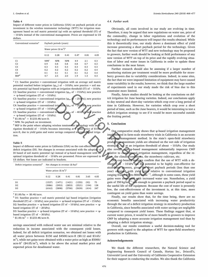
savings associated with reduced water use are minimal relative to thereduction in income associated with the consequent yield losses.Indeed, for all deficit irrigation scenarios, we obtained net losses withall water prices between $150 and $4500/acre-ft ($0.12 and $3.65/m3), while net gains were obtained with a water price as high as $5000/acre-ft1 ($4.05/m3), which is far above the actual market price andexpected prices for desalinated water.

4.4. Further work

Obviously, all costs involved in our study are evolving in time.Therefore, it may be argued that new regulations on water use, price ofthe commodity, change in labor regulations and evolution of thetechnology and its performances will impact the results obtained. Whilethis is theoretically true, our study shows a dominant effect of yieldincrease generating a short payback period for the technology. Giventhe fact that new version of WTT and new technology may be proposedto growers, further work should be looking at field performance of anynew version of WTT on top of its price and the rapidly evolving situa-tion of labor and water issues in California in order to update theseconclusions in the near future.

Further research should also be assessing if a larger number ofmonitoring stations per treatment would be more profitable for straw-berry growers due to variability considerations. Indeed, in some sites,the fact that we were imposed limitation of equipment may have causedsome variability in the results; however, we think that the large numberof experiments used in our study made the risk of bias due to thisconstraint more limited.

Finally, future studies should be looking at the conclusions on def-icit irrigation for June bearing varieties. Indeed, our conclusions applyto day neutral and short-day varieties which crop over a long period oftime in California. However, for varieties which crop over a shortperiod of time, such as the June bearers, it would be interesting to test adeficit irrigation strategy to see if it would be more successful outsidethe fruiting period.

5. Conclusion

Our comparative study shows that ѱ-based irrigation managementimplemented in farm-scale strawberry trials in California is an accurateirrigation management method. In the state’s open-field strawberryproduction, maximum yields are obtained on the wet side of irrigationstrategies, i.e. at an irrigation threshold of about −10 kPa. Our studyalso reveals that ѱ-based management substantially improves CWPrelative to conventional irrigation management, regardless of the re-gion, the climatic conditions, the strawberry cultivars, etc.

Our cost-benefit analyses confirm that the use of WTT with a de-fined IT of −10 kPa has the potential to be highly cost-effective forstrawberry growers, given the short payback periods (less than oneyear) obtained with yield gains relative to conventional irrigationranging from 1440 to 8660 kg·ha−1, although in some cases, these yieldgains were associated with increased water use. Nonetheless, a yieldgain of 350 kg·ha−1 was enough to generate a payback period equal tothe useful life of the equipment. Because the cost of water is presentlylow, the cost-effectiveness of the investment is, at this time, morecontingent on yield gains than water savings.

Finally, our results show that, for the time being, there are noeconomic benefits associated with increasing water productivitythrough the use of a deficit irrigation strategy in strawberry productionin California, since benefits associated with water savings are negligiblecompared to consequent yield losses. These findings suggest that, atcurrent water prices, it would be of more benefit to growers to improveCWP by adopting a more accurate irrigation management tool than byadopting a deficit irrigation strategy.

Overall, our results constitute a useful decision-making tool forgrowers with regard to the adoption of WTT for open-field strawberryproduction in California.

Acknowledgements

We thank the different researchers, the Natural Science andEngineering Research Council of Canada, Hortau Inc., Driscoll’s,Université Laval and the University of California Cooperative Extensionfor their support in conducting the studies. We also thank the California

Table 4Impact of different water prices in California (USA) on payback periods of aninvestment in the wireless tensiometer technology (WTT) for irrigation man-agement based on soil matric potential (ѱ) with an optimal threshold (IT) of−10 kPa instead of the conventional management. Prices are expressed in USdollars.

Conventional scenariosa Payback periods (years)

Water prices ($/m3)b

0.12 0.28 0.41 0.47 0.81 4.05

C1 NPBc NPB NPB 4.9 2.1 0.3C2 0.9 0.8 0.8 0.8 0.7 0.3C3 0.3 0.3 0.3 0.3 0.3 0.3C4 0.2 0.2 0.2 0.2 0.2 0.4C5 0.1 0.1 0.1 0.1 0.2 0.4BEPd 4.7 2.5 2.0 1.9 1.3 0.3

a C1: baseline practice= conventional irrigation with an average soil matricpotential reached before irrigation (ѱirr) of −10 kPa; new practice= soil ma-tric potential (ѱ)-based irrigation with an irrigation threshold (IT) of −10 kPa.C2: baseline practice= conventional irrigation (ѱirr of −15 kPa); new practice= ѱ-based irrigation (IT of −10 kPa).C3: baseline practice= conventional irrigation (ѱirr of −25 kPa); new practice= ѱ-based irrigation (IT of −10 kPa).C4: baseline practice= conventional irrigation (ѱirr of −35 kPa); new practice= ѱ-based irrigation (IT of −10 kPa).C5: baseline practice= conventional irrigation (ѱirr of −40 kPa); new practice= ѱ-based irrigation (IT of −10 kPa).b $1.00/m3 = $1233.48/acre-ft.c NPB: No payback on investment.d BEP is the point where adopting wireless tensiometer technology with an ir-rigation threshold of −10 kPa becomes interesting at a water price of $150/acre-ft, due to yield gains and water savings compared to conventional irriga-tion.

Table 5Impact of different water prices in California (USA) on the cost-effectiveness ofdeficit irrigation (DI). Net changes in revenue associated with the adoption ofDI based of soil matric potential (ѱ) instead of ѱ-based management with anoptimal irrigation threshold of −10 kPa are presented. Prices are expressed inUS dollars. Net losses are indicated in brackets.

Deficit irrigation scenariosb Net changes in revenue ($/ha)a

Water prices ($/m3)c

0.12 0.28 0.41 0.81 3.65 4.05

D1 (1537) (1471) (1421) (1255) (92) 75D2 (3086) (2953) (2853) (2521) (194) 138D3 (6162) (5898) (5700) (5039) (414) 247

a $1.00/ha = $0.40/acre.b D1: baseline practice= soil matric potential (ѱ) based irrigation [irrigationthreshold (IT) of −10 kPa]; new practice = ѱ-based irrigation (IT of −15 kPa).D2: baseline practice = ѱ-based irrigation (IT of −10 kPa); new practice = ѱ-based irrigation (IT of −20 kPa).D3: baseline practice = ѱ-based irrigation (IT of −10 kPa); new practice = ѱ-based irrigation (IT of −30 kPa).c $1.00/m3 = $1233.48/acre-ft.

L. Gendron et al. Scientia Horticulturae 240 (2018) 468–477

476

Only for Reading

Do not Download

growers for providing the experimental sites, material and workforce.

Supplementary data.

Supplementary material related to this article can be found, in theonline version, at doi:https://doi.org/10.1016/j.scienta.2018.06.013.

References

Aiken, L.S., West, S.G., Reno, R.R., 1991. Multiple Regression: Testing and InterpretingInteractions, first ed. Thousand Oaks.

Allen, R.G., Pereira, L.S., Raes, D., Smith, M., 1998. Crop evapotranspiration: guidelinesfor computing crop water requirements. FAO Irrig. Drain. Pap. 56, 1–15.

Anderson, L., 2015. Détermination de la stratégie d’irrigation optimale de la fraise baséesur le potentiel matriciel du sol et un modèle climatique. MS Thesis. Univ. Laval,Quebec.

Arnold, T., 2014. How Net Present Value Is Implemented in: A Pragmatic Guide to RealOptions. Palgrave Macmillan US, New York, pp. 1–13. http://dx.doi.org/10.1057/9781137391162_1.

Cahn, M.D., Smith, R.F., Farrara, B.F., Hartz, T.K., Johnson, L.F., Melton, F.S., Post, K.M.,2016. Irrigation and nitrogen management decision support tool for vegetables andberries. Groundw. Issues Water Manag. 53–63.

California Department of Water Resources, 2014. Public Update for Drought Response.California Dep. of Water Resour., Sacramento.

California Irrigation Management Information System (CIMIS), 2017. CIMIS Overview -Data Retrieval by Users. 15 April 2016. http://wwwcimis.water.ca.gov/Default.aspx.

Chappell, M., Dove, S.K., Van Iersel, M.W., Thomas, P.A., Ruter, J., 2013. Implementationof wireless sensor networks for irrigation control in three container nurseries.HortTechnology 23 (6), 747–753.

Coelho, E.F., Or, D., 1998. Root distribution and water uptake patterns of corn undersurface and subsurface drip irrigation. Plant Soil 206 (2), 123–136. http://dx.doi.org/10.1023/A:1004325219804.

El-Farhan, A.H., Pritts, M.P., 1997. Water requirements and water stress in strawberry.Advances Strawb. Res. 16, 5–12.

FAOSTAT, 2016. Food and Agricultural Commodities Production, Countries byCommodity. 24 May 2016. http://faostat3.fao.org/browse/rankings/countries_by_commodity/E.

Fereres, E., Soriano, M.A., 2007. Deficit irrigation for reducing agricultural water use. J.Exp. Bot. 58 (2), 147–159. http://dx.doi.org/10.1093/jxb/erl165.

Fulcher, A., LeBude, A.V., Owen Jr., J.S., White, S.A., Beeson, R.C., 2016. The next tenyears: strategic vision of water resources for nursery producers. HortTechnology 26(2), 121–132.

Gallardo, M., Snyder, R.L., Schulbach, K., Jackson, L.E., 1996. Crop growth and water usemodel for lettuce. J. Irrig. Drain. Eng. 1996 (November-December), 354–359.

Gaudin, M., Jaffrès, C., Réthoré, A., 2011. Gestion de l’exploitation agricole, third ed.Paris.

Geerts, S., Raes, D., 2009. Deficit irrigation as an on-farm strategy to maximize crop waterproductivity in dry areas. Agric. Water Manage. 96 (9), 1275–1284. http://dx.doi.org/10.1016/j.agwat.2009.04.009.

Gendron, L., Létourneau, G., Depardieu, C., Anderson, L., Sauvageau, G., Levallois, R.,Caron, J., 2017. Irrigation management based on soil matric potential improveswater use efficiency of field-grown strawberries in California. Acta Hortic. 1156,191–196. http://dx.doi.org/10.17660/ActaHortic.2017.1156.29.

Grattan, S.R., Bowers, W., Dong, A., Snyder, R.L., Carroll, J.J., George, W., 1998. Newcrop coefficients estimate water use of vegetables, row crops. Calif. Agric. 52 (1),16–21. http://dx.doi.org/10.3733/ca.v052n01p16.

Gray, B., Hanak, E., Frank, R., Howitt, R., Lund, J., Szeptycki, L., Thompson, B., 2015.Allocating California’s Water: Directions for Reform. Public Policy Institute of Calif.,PPIC Water Policy Center, San Francisco.

Guimerà, J., Marfà, O., Candela, L., Serrano, L., 1995. Nitrate leaching and strawberryproduction under drip irrigation management. Agr. Ecosyst. Environ. 56, 121–135.http://dx.doi.org/10.1016/0167-8809(95)00620-6.

Hanson, H.C., 1931. Comparison of root and top development in varieties of strawberry.Am. J. Bot. 18 (8), 658. http://dx.doi.org/10.2307/2435677.

Hanson, B., Bendixen, W., 2004. Drip irrigation evaluated in Santa Maria Valley straw-berries. Calif. Agric. 58 (1), 48–53 http://doi.org/10.3733.

Hoppula, K.I., Salo, T.J., 2007. Tensiometer-based irrigation scheduling in perennialstrawberry cultivation. Irr. Sci. 25, 401–409. http://dx.doi.org/10.1007/s00271-006-0055-7.

Lea-Cox, J.D., 2012. Using wireless sensor networks for precision irrigation scheduling.In: Kumar, M. (Ed.), Problems, Perspectives and Challenges of Agricultural WaterManagement. In Tech Publisher, London, pp. 233–258.

Lea-Cox, J.D., Bauerle, W.L., Iersel, M.W., van, Kantor, G.F., Bauerle, T.L., Lichtenberg, E.,King, D.M., Crawford, L., 2013. Advancing wireless sensor networks for irrigationmanagement of ornamental crops: an overview. HortTechnology 23 (6), 717–724.

Létourneau, G., Caron, J., Anderson, L., Cormier, J., 2015. Matric potential-based irri-gation management of field-grown strawberry: effects on yield and water use effi-ciency. Agr. Water Mgt. 161, 102–113. http://dx.doi.org/10.1016/j.agwat.2015.07.005.

Levallois, R., 2010. Gestion de l’entreprise agricole : de la théorie à la pratique, first ed.Quebec.

Majsztrik, J., Lichtenberg, E., Saavoss, M., 2013. Ornamental grower perceptions ofwireless irrigation sensor networks: results from a national survey. HortTechnology23 (6), 775–782.

Migliaccio, K.W., Schaffer, B., Li, Y.C., Evans, E., Crane, J.H., Muñoz-Carpena, R., 2008.Assessing benefits of irrigation and nutrient management practices on a southeastFlorida royal palm (Roystonea elata) field nursery. Irrig. Sci. 27 (1), 57–66. http://dx.doi.org/10.1007/s00271-008-0121-4.

Manitoba Ministery of Agriculture, Food and Rural Development, 2015. StrawberryIrrigation. Water Interrelations. 10 November 2017. http://www.gov.mb.ca/agriculture/crops/production/fruit-crops/strawberry-irrigation.html.

Muñoz-Carpena, R., Bryan, H., Klassen, W., Dukes, M.D., 2003. Automatic soil moisture-based drip irrigation for improving tomato production. Proc. Fla. State. Hort. Soc.116, 80–85.

Penson, J.B., Capps, O., Rosson, C.P., 2002. Introduction to Agricultural Economics, 3rded. Prentice Hall, Upper Saddle River, N.J.

Peñuelas, J., Savé, R., Marfà, O., Serrano, L., 1992. Remotely measured canopy tem-perature of greenhouse strawberries as indicator of water status and yield under mildand very mild water stress conditions. Agric. For. Meteorol. 58, 63–77. http://dx.doi.org/10.1016/0168-1923(92)90111-G.

Saleem, S.K., Delgoda, D.K., Ooi, S.K., Dassanayake, K.B., Liu, L., Halgamuge, M.N.,Malano, H., 2013. Model predictive control for real-time irrigation scheduling. IFACAgricontrol 4, 299–304. http://dx.doi.org/10.3182/20130828-2-SF-3019.00062.

Scanlon, B.R., Faunt, C.C., Longuevergne, L., Reedy, R.C., Alley, W.M., McGuire, V.L.,McMahon, P.B., 2012. Groundwater depletion and sustainability of irrigation in theUS high plains and Central Valley. Proc. Natl. Acad. Sci. 109 (24), 9320–9325. http://dx.doi.org/10.1073/pnas.1200311109.

Serrano, L., Carbonell, X., Savé, R., Marfà, O., Peñuelas, J., 1992. Effects of irrigationregimes on the yield and water use of strawberry. Irrig. Sci. 13 (1), 45–48. http://dx.doi.org/10.1007/BF00190244.

Shae, J.B., Steele, D.D., Gregor, B.L., 1999. Irrigation scheduling methods for potatoes inthe Northern Great plains. Trans. ASAE 42 (2), 351–360. http://dx.doi.org/10.13031/2013.13366.

Strand, L., 2008. Integrated Pest Management for Strawberries, second ed. United States.U.S. Department of Agriculture (USDA), 2013. 2012 Census of Agriculture, U.S.

Strawberry Harvested Acreage, Yield Per acre, and Production, 13 States, 1970-2013.U.S. Dept. Agr., Washington, D.C.

USDA, 2016. California Drought: Farms. 13 August 2016. aspx in August 2016. http://www.ers.usda.gov/topics/in-the-news/california-drought-farm-and-food-impacts/california-drought-farms.

Yuan, B., Sun, J., Nishiyama, S., 2004. Effect of drip irrigation on strawberry growth andyield inside a plastic greenhouse. Biosyst. Eng. 87 (2), 237–245. http://dx.doi.org/10.1016/j.biosystemseng.2003.10.014.

Zwart, S.J., Bastiaanssen, W.G.M., 2004. Review of measured crop water productivityvalues for irrigated wheat, rice, cotton and maize. Agric. Water Manag. 69 (2),115–133. http://dx.doi.org/10.1016/j.agwat.2004.04.

L. Gendron et al. Scientia Horticulturae 240 (2018) 468–477

477