real-time data assimilation for operational ensemble...

Real-Time Data Assimilation for Operational Ensemble Streamflow Forecasting

JASPER A. VRUGT

Earth and Environmental Sciences Division, Los Alamos National Laboratory, Los Alamos, New Mexico

HOSHIN V. GUPTA

Department of Hydrology and Water Resources, The University of Arizona, Tucson, Arizona

BREANNDÁN Ó NUALLÁIN

Department of Computational Science, University of Amsterdam, Amsterdam, Netherlands

WILLEM BOUTEN

Department of Physical Geography and Soil Science, University of Amsterdam, Amsterdam, Netherlands

(Manuscript received 16 March 2005, in final form 15 September 2005)

ABSTRACT

Operational flood forecasting requires that accurate estimates of the uncertainty associated with model-generated streamflow forecasts be provided along with the probable flow levels. This paper demonstratesa stochastic ensemble implementation of the Sacramento model used routinely by the National WeatherService for deterministic streamflow forecasting. The approach, the simultaneous optimization and dataassimilation method (SODA), uses an ensemble Kalman filter (EnKF) for recursive state estimation al-lowing for treatment of streamflow data error, model structural error, and parameter uncertainty, whileenabling implementation of the Sacramento model without major modification to its current structuralform. Model parameters are estimated in batch using the shuffled complex evolution metropolis stochastic-ensemble optimization approach (SCEM-UA). The SODA approach was implemented using parallel com-puting to handle the increased computational requirements. Studies using data from the Leaf River, Mis-sissippi, indicate that forecast performance improvements on the order of 30% to 50% can be realized evenwith a suboptimal implementation of the filter. Further, the SODA parameter estimates appear to be lessbiased, which may increase the prospects for finding useful regionalization relationships.

1. Introduction and scope

Since the early 1960s, considerable effort has beendevoted to the development and application of modelsof the rainfall–runoff process. A class of these, oftencalled “conceptual watershed models” represents theprecipitation–soil moisture–streamflow water balancedynamics using heuristic and/or empirical relationshipsthat represent a perceptual and conceptual hydrologicunderstanding of watershed behavior at aggregatescales (see, e.g., Kuczera 1997). Conceptual watershed

models used for operational streamflow forecastingtypically have 10 or more parameters that specify thebehavior of the transfer functions relating inputs to out-puts via series and parallel pathways of interconnectedconceptual water storages (state variables) representingsoil moisture accumulations in the upper and lower soilzones. It is tacitly assumed that these conceptual stor-ages correspond to “real” control volumes in physicalspace, even though the boundaries of these control vol-umes cannot generally be explicitly delineated.

The Sacramento Soil Moisture Accounting concep-tual watershed model (SAC-SMA; Burnash et al. 1973)is used by the National Weather Service (NWS) foroperational streamflow forecasting and flood warningthroughout the United States. The model has 16 pa-rameters whose values must be specified (Table 1).

Corresponding author address: Jasper Vrugt, Earth and Envi-ronmental Science Division, Los Alamos National Laboratory,Los Alamos, NM 87544.E-mail: [email protected]

548 J O U R N A L O F H Y D R O M E T E O R O L O G Y VOLUME 7

© 2006 American Meteorological Society

JHM504

While the values of some of these parameters can beestimated directly from knowledge of physical water-shed characteristics, most represent “effective” water-shed properties that cannot, in practice, be measuredvia direct observation in the field. It is common prac-tice, therefore to estimate values for the model param-eters by calibrating the performance of the modelagainst a historically observed streamflow hydrograph,using either a “manual expert” trial-and-error approachor an automated search algorithm (e.g., Gupta et al.1998; Boyle et al. 2000; Madsen 2000). Note that pa-rameters estimated in this manner are spatially andtemporally lumped (i.e., effective) representations ofheterogeneous watershed properties.

While considerable progress has been made in thedevelopment and application of automated proceduresfor watershed model calibration, such methods havereceived criticism for their lack of rigor in treating vari-ous sources of uncertainty (e.g., Beven and Binley 1992;Thiemann et al. 2001; Vrugt et al. 2005). In particular,most procedures explicitly account only for uncertain-ties in the streamflow measurement data (e.g., So-rooshian and Dracup 1980; Sorooshian et al. 1993) andin the parameter estimates (e.g., Kuczera 1983a,b;

Beven and Binley 1992; Gupta et al. 1998; Thiemann etal. 2001; Vrugt et al. 2003b, 2006a). Most methods usebatch processing of the data to search for parameterestimates that minimize a likelihood measure of theoverall (statistical) variance of the model residuals. Un-certainties that stem from errors associated with themeasured system inputs (rainfall and potential evapo-transpiration), initialization and propagation of statevariables (moisture storages), and model structural er-rors arising from inadequate representation of physicalprocesses (including the aggregation of spatially distrib-uted processes) have not been adequately handled in anexplicit manner.

Over the past decade, interesting methods for ad-dressing such problems have appeared in the literature,with attention given to the problem of estimating rea-sonable uncertainty bounds on the model predictions.Bayesian, pseudo-Bayesian, set-theoretic, multiple-criteria, and recursive model identification strategiesthat estimate model parameter and streamflow predic-tion uncertainties can provide forecasts of the “mostprobable” streamflow value along with estimates of theranges of possible outcomes (e.g., Kuczera 1983a,b;Keesman 1990; van Straten and Keesman 1991; Beven

TABLE 1. Parameter and state variables in the SAC-SMA model.

Capacity thresholdsInitialranges

SCEM-UAranges

SODAranges

UZTWM Upper-zone tension water maximum storage (mm) 1.0–150.0 90.2–91.1 85.8–129.3UZFWM Upper-zone free water maximum storage (mm) 1.0–150.0 16.3–16.8 66.5–93.6LZTWM Lower-zone tension water maximum storage (mm) 1.0–500.0 267.6–270.2 121.2–155.3LZFPM Lower-zone free water primary maximum storage (mm) 1.0–1000.0 141.8–148.2 384.6–730.4LZFSM Lower-zone free water supplemental maximum storage (mm) 1.0–1000.0 51.0–53.9 180.0–557.4ADIMP Additional impervious area (�) 0.0–0.40 0.08–0.10 0.38–0.40

Recession parametersUZK Upper-zone free water lateral depletion rate (day�1) 0.1–0.5 0.50–0.50 0.32–0.46LZPK Lower-zone primary free water depletion rate (day�1) 0.0001–0.025 0.001–0.001 0.0006–0.004LZSK Lower-zone supplemental free water depletion rate (day�1) 0.01–0.25 0.06–0.07 0.18–0.19

Percolation and otherZPERC Maximum percolation rate (�) 1.0–250.0 248.9–250.0 4.5–94.8REXP Exponent of the percolation equation (�) 1.0–5.0 2.6–2.7 1.2–2.1PCTIM Impervious fraction of the watershed area (�) 0.0–0.1 0.007–0.007 0.04–0.05PFREE Fraction percolating from upper- to lower-zone free

water storage(�) 0.0–0.6 0.13–0.13 0.37–0.44

Not optimizedRIVA Riparian vegetation area (�) 0.0SIDE Ratio of deep recharge to channel base flow (�) 0.0RSERV Fraction of lower zone free water not transferable to

tension water(�) 0.3

States DescriptionUZTWC Upper-zone tension water storage content (mm)UZFWC Upper-zone free water storage content (mm)LZTWC Lower-zone tension water storage content (mm)LZFPC Lower-zone free primary water storage content (mm)LZFSC Lower-zone free secondary water storage content (mm)ADIMC Additional impervious area content (mm)

JUNE 2006 V R U G T E T A L . 549

and Binley 1992; Klepper et al. 1991; Freer et al. 1996;Gupta et al. 1998; Thiemann et al. 2001; Young 2001;Vrugt et al. 2003b, 2006a). Such methods typically sum-marize the model uncertainty primarily in terms of un-certainty in the parameter estimates.

Since the early 1980s, state-space filtering methodshave been proposed as having the potential for explic-itly handling uncertainties in hydrological models. Incontrast to classical model calibration strategies, state-space filtering methods continuously update the statesin the model when new measurements become avail-able, to improve the model forecast and estimate fore-cast accuracy. Variations of the Kalman filter approach(Kalman 1960) have been applied to real-time stream-flow forecasting by Todini et al. (1976), Kitanidis andBras (1980a,b), Bras and Restrepo-Posada (1980), Brasand Rodriguez-Iturbe (1985), Wood and O’Connell(1985), Awwad and Valdés (1992), Awwad et al. (1994),and Young (2002), among others. Of particular rel-evance to this paper is the pioneering work of Kitanidisand Bras (1980a,b) in which an extended Kalman filter(EKF) was implemented using a state-space reformu-lation of the nonlinear SAC-SMA model to trackprobabilistic estimates of the state variables and to de-tect impulse-type rainfall errors. However, the recur-sive KF approach did not achieve practical operationalstatus for a variety of practical reasons, an importantone being that the implementation requires the highlynonlinear original model to be rendered into a continu-ously differentiable state-space form, involving variousmodifications and/or approximations (Kitanidis andBras 1980a,b; Georgakakos et al. 1988; Georgakakosand Sperflage 1995; Refsgaard 1998; Seo et al. 2003).Besides the fact that the input-state-output behavior ofthe reformulated state-space model can deviate signifi-cantly from the original model—the EKF is notoriouslyunstable if the model nonlinearities are strong (Even-sen 1992; Miller et al. 1994)—the model reformulationand the computation of model derivative equations canrequire a considerable amount of experience and ex-pertise (Seo et al. 2003). Further, the computationalcosts of state-space filtering methods (e.g., KF andEKF) are significant (especially for high-dimensionalstate-vector problems, such as spatially distributedmodels) and have, so far, restricted their widespreadimplementation for operational use.

Other data assimilation approaches have been re-cently explored. Seo et al. (2003) investigated varia-tional assimilation (VAR) as a tool for assimilating cli-matological estimates of potential evaporation andreal-time observations of streamflow and precipitationto improve SAC-SMA model streamflow forecasts. TheVAR method has achieved widespread application to

hydrometeorological and oceanographic models anddoes not depend on a state-space model formulation,but does require availability of an adjoint code that canbe difficult to derive. Hydrological investigations ofVAR include the work of Reichle et al. (2001) for es-timating spatial soil-moisture distributions by assimila-tion of remotely sensed microwave brightness tempera-tures into a land surface model. Madsen and Skotner(2005) investigated the suboptimal steady Kalman filterapproximation of Cañizares et al. (2001) for adaptivestate updating using the Mike-11 model and reportedthat the reduced computational costs make the methodbetter suited than the full Kalman filter for operationaluse.

In the past few years, ensemble forecasting tech-niques based on sequential data assimilation (SDA)methods have become increasingly popular due to theirpotential ability to explicitly handle the various sourcesof uncertainty in operational hydrological models.Early techniques reported in the literature include thedynamic identifiability analysis approach for recursiveidentifiability and detection of time variation in modelparameters (DYNIA; Wagener et al. 2003), the param-eter identification method based on localization of in-formation (PIMLI; Vrugt et al. 2002), and the Bayesianrecursive estimation approach (BaRE; Thiemann et al.2001; Misirli 2003; Gupta et al. 2003). Most recently,techniques based on the ensemble Kalman filter(EnKF; Evensen 1994) have been suggested as havingthe power and flexibility required for data assimilationusing conceptual watershed models. Vrugt et al. (2005)presented the simultaneous optimization and data as-similation method (SODA), which uses EnKF to recur-sively update model states while estimating time-inva-riant values for the model parameters using the shuffledcomplex evolution metropolis stochastic-ensemble op-timization approach (SCEM-UA; Vrugt et al. 2003b).A novel feature of SODA is its explicit treatment oferrors due to parameter uncertainty, state variables’uncertainty, model structural error, and streamflowmeasurement error. Moradkhani et al. (2005a,b) pre-sented two different dual state-parameter estimation(DSPE) methods based on EnKF and sequential MonteCarlo techniques [SMC; also known as particle filtering(e.g., Gordon et al. 1993; Arulampalam et al. 2002)],respectively, for simultaneous recursive time-variableestimation of model states and parameters. Both EnKFand SMC allow accurate tracking of second-order mo-ments of the probability distribution functions for mod-els having nonlinear dynamics, but SMC can also trackhigher moments and therefore incurs increased compu-tational costs. The EnKF achieves better computationalefficiency by using linear rules for state updating but


may give suboptimal performance in the presence ofstrong model nonlinearities.

The objective of this paper is to investigate the ap-plicability and advantages of using SODA for joint pa-rameter-state estimation and ensemble streamflowforecasting using the operational SAC-SMA concep-tual watershed model. Our motivation is that theSODA method has the potential for ready assimilationinto NWS operational forecasting procedures, therebyproviding stochastic streamflow forecasts without re-quiring significant modifications to operational modelcodes or software. The paper is organized as follows.Section 2 presents a brief description of the SAC-SMAmodel. Sections 3 and 4 discuss the rationale and archi-tecture of SODA and its implementation using parallelcomputing. Sections 5 and 6 present the experimentaldesign and data used in this study and discuss the find-ings and results. In particular, we compare the per-formance of the stochastic SODA method with theconventional deterministic approach in current opera-tional usage. Finally, section 7 summarizes the resultsand conclusions and explores implications for futurework.

2. Sacramento Soil Moisture Accounting model

The SAC-SMA model (Fig. 1) is a lumped concep-tual watershed model consisting of six state variablereservoirs representing the accumulation of water intwo soil zones (upper and lower), in the forms of both“tension” and “free” water (Burnash et al. 1973; Braziland Hudlow 1981). The upper zone represents surfacesoil processes and interception storage, while the lowerzone represents deeper soil processes and groundwaterstorage. Nonlinear equations relate the absolute andrelative quantities of water within the state variablereservoirs and control the partitioning of precipitationinto overland flow, infiltration to the upper zone, inter-flow, percolation to the lower zone, and fast and slowcomponents of groundwater recession baseflow. Satu-ration excess overland flow occurs when rainfall ex-ceeds the interflow and percolation capacities and theupper zone storage is full. Percolation from the upperto the lower layer is controlled by a complex nonlinearprocess dependent on the storages in both soil zones.

The model has 13 user-specifiable (and 3 fixed) pa-rameters and an evapotranspiration demand curve (or

FIG. 1. Schematic representation of the SAC-SMA model as implemented in this study. The rectangles refer to the various modelstates, while arrows indicate fluxes between compartments; Z1, Z2, and Z3 refer to the three main channel components, which sumtogether to become the streamflow Z at the watershed outlet.

JUNE 2006 V R U G T E T A L . 551

adjustment curve). Inputs to the model include meanareal precipitation (MAP) and potential evapotranspi-ration (PET) while the outputs are estimated evapo-transpiration and channel inflow. A unit hydrograph orkinematic wave routing model is commonly used torout channel inflow downstream to the gauging point.In this work, we instead use a simple Nash cascade(NC) of three linear reservoirs to rout the upper zone(quick response) channel inflow (Z1) while the lowerzone recession components Z2 and Z3 are passed di-rectly to the gauging point. This configuration adds oneparameter and three state variables to the model, butfacilitates inclusion of the NC routing model parameterand states in the data assimilation process. Moreover,NC routing considerably improves computational timeas it avoids the need for computationally expensiveconvolution. Our formulation of the model thereforehas 14 time-invariant parameters and 9 time-varyingstate variables to be estimated.

The SAC-SMA model has been used extensively inprevious studies to study automatic model calibrationissues (e.g., Brazil and Hudlow 1981; Sorooshian andGupta 1983; Gupta and Sorooshian 1985; Sorooshian etal. 1993; Gupta et al. 1998; Boyle et al. 2000, 2001;Hogue et al. 2000, 2005; Thiemann et al. 2001; Vrugt etal. 2003a, 2006a; among others) and to explore stateestimation for improved streamflow forecasting (e.g.,Kitanidis and Bras 1980a,b; Seo et al. 2003).

3. Simultaneous optimization and data assimilation

Conventional methods for automated calibration ofnonlinear watershed models treat the underlying uncer-tainty in the input-state-output representation of themodel as arising primarily from uncertainty in the pa-rameter estimates and output measurements. That ap-proach essentially neglects measurement errors associ-ated with the system input (forcing), state variables,and model structure leading to model simulations andassociated prediction uncertainty bounds that do notconsistently and accurately simulate the observed un-certainty in system behavior (Vrugt et al. 2005). This iseasily seen by examination of the model residuals,which typically exhibit considerable variation in bias(nonstationarity), variance (heteroscedasticity), andcorrelation structure under different hydrologic condi-tions. Several contributions to the hydrologic literaturehave brought into question the continued usefulness ofthe classical paradigm for estimating model parameters(see, e.g., Beven and Binley 1992; Gupta et al. 1998;Kavetski et al. 2003).

In a separate line of research considerable progresshas been made in the development and application of

SDA techniques, which provide a general and explicitframework for dealing with input, output, and modelstructural uncertainties but assume the optimal modelparameters to be known a priori. The latter assumptionis particularly inappropriate for conceptual watershedmodels, in which the parameters represent lumped andaggregated processes in space and time that cannot bemeasured directly and are therefore poorly specified. Ithas been our experience that considerable uncertaintyin the state values and associated model output predic-tion can arise due to uncertainty in the choice of pa-rameter values.

Vrugt et al. (2005) recently proposed the combineduse of parameter optimization and sequential data as-similation to facilitate improved treatment of input,output, parameter, and model structural errors in hy-drologic modeling using an algorithm named SODA.The algorithm merges the strengths of the SCEM-UAstochastic parameter optimization method with thepower and computational efficiency of EnKF to simul-taneously estimate both state variables and parameters.For detailed descriptions of EnKF and SODA seeEvensen (1994) and Vrugt et al. (2005), respectively. Inbrief, SODA implements an inner EnKF loop for re-cursive state estimation (conditioned on an assumedparameter set) within an outer stochastic global opti-mization loop for batch estimation of the posterior den-sity of the parameters. The EnKF uses a Monte Carlo–based randomly sampled ensemble of state trajectoriesto propagate and update approximate estimates of themean and covariance of the uncertain state variables �t

from one time step to the next. See Fig. 2 for a con-densed outline of the method. A key point is that theEnKF propagates an ensemble of state-vector trajecto-ries in parallel such that each trajectory represents onerealization of generated model replicates. When an out-put measurement is available, each forecasted en-semble state vector � f

t is updated to �ut by means of a

linear updating rule (in a manner analogous to the Kal-man filter):

� tu � � t

f � Kt��z̃t � H�� tf ��, �1�

where z̃t denotes a streamflow observation from datasetZ̃ � {z̃1, . . . , z̃n}, H(•) represents the operator relatingthe model states to the model output, and the strengthof the gain Kt depends on the strength of the crosscovariance between the state variables of interest andthe model outputs for which measurements are avail-able. The cross covariance is approximated using theinformation contained in the ensembles. It should benoted, therefore, that the EnKF updating strategy fa-vors situations for which the state to output transition


equations are weakly nonlinear or almost linear overthe range of conditions spanned by the ensembles, andfor cases where the state–output relationships arestrongly nonlinear, the EnKF may not be useable forstate updating.

For parameter estimation, a Bayesian criterion isspecified (Box and Tiao 1973) that measures the “close-ness” between the (EnKF derived) mean ensemblemodel forecast and the corresponding measurement,resulting in the posterior density function:

p��|Z̃� � t�1

n

�et��n, �2�

where n denotes the total number of streamflow obser-vations, and et(�) represents the mean ensemblestreamflow forecast error computed at each measure-ment time t as

et�� z̃t � H�� tf��. �3�

To generate parameter samples corresponding to thedistribution indicated by the posterior parameter prob-ability density function [Eq. (2)], we use an implemen-tation of the general purpose SCEM-UA global opti-mization algorithm, which provides an efficient esti-mate of the posterior distribution and its mode (the

FIG. 2. Flowchart of the EnKF used in SODA to recursively estimate the state variables; Ndenotes the ensemble size, n the number of time steps, � is the SCEM-UA generated param-eter combination, and �o represents the error covariance of the observations.

JUNE 2006 V R U G T E T A L . 553

most likely parameter set) within a single optimizationrun (Vrugt et al. 2003b). The algorithm, a modifica-tion of the successful SCE-UA global optimiza-tion method (Duan et al. 1992, 1994), belongs to thefamily of Markov chain Monte Carlo (MCMC) sam-plers, and generates multiple sequences of parametersets {�(1), �(2), . . . , �(k�1)} that converge to the station-ary posterior distribution. Studies using a parsimoniousfive-parameter conceptual watershed model haveshown that SODA leads to improved estimates of pa-rameter and model output prediction uncertainty(Vrugt et al. 2005).

4. Implementation using parallel computing

Implementation of the SODA methodology requiresthe EnKF solution of a sequential state estimationproblem (over the calibration period) for each SCEM-UA generated parameter set. Approximation of thestochastic evolution of the state error covariance matrixtherefore involves large numbers of deterministic wa-tershed model simulation runs. Fortunately, there hasbeen considerable progress in the development of dis-tributed computer systems using the power of multipleprocessors to efficiently solve large computationalproblems. In hydrology, many computational problemsrelated to the flow and storage of water are admirablysuited for implementation on distributed computer sys-tems.

In this study, we implemented the SODA methodol-ogy using a local area multi-computer (LAM)/messagepassing interface (MPI) distributed computing interfacefor the Octave programming environment (Vrugt et al.2006b). LAM/MPI is a high-quality open-source imple-mentation of the message passing interface specifica-tion, including all of MPI-1.2 and much of MPI-2. In-tended for production as well as research use, LAM/MPI includes a rich set of features for parallelcomputing. GNU Octave (Eaton 1998, 2001) is a high-level language intended primarily for numerical com-putation. It provides a convenient command line inter-face for numerical solution of linear and nonlinearproblems, and for performing numerical experi-ments, using a language that is highly compatible withMATLAB. A detailed description and explanation ofthe software appear in Fernández et al. (2003, 2004).

Our parallel computing implementation of SODA in-corporates some minor modifications to the sequentialnature in which the samples are generated within eachMarkov chain of the SCEM-UA algorithm. A flowchartof our parallel implementation is given in Fig. 3. First,the evaluation of the fitness function for the individualsin the population is distributed over the slave proces-

sors, thereby avoiding excessively long execution timeson a single processor. Second, each slave computer(node) is set up to evolve a different sequence andcomplex in the SCEM-UA algorithm, as this step doesnot require information exchange and communicationbetween different nodes. Each node might therefore beconsidered as a “particle” within the state space, evolv-ing each of the SCEM-UA Markov chains to explorethe global parameter space. The calculations reportedin this paper were implemented using 25 Pentium IV3.40-GHz processors of the LISA cluster belonging tothe SARA parallel computing center (Netherlands).The CPU time required for joint stochastic calibrationand ensemble state estimation of the SAC-SMA modelusing 8 yr of daily streamflow data and 50 000 SCEM-UA generated parameters combinations was approxi-mately 22 h.

5. Experimental design and data used

The watershed used for this study is the Leaf Riverbasin in Mississippi for which approximately 40 yr ofhistorical 6-hourly MAP and daily streamflow and PETdata are available. Previous work has indicated that acalibration dataset of approximately 8 to 11 yr of data,representing a range of hydrologic phenomena (wet,medium, and dry years), is desirable to achieve deter-ministic model calibrations that are consistent and gen-erate good verification and forecasting performance(e.g., Yapo et al. 1996; Vrugt et al. 2006a). In this studywe use 8 yr [water years (WY) 1953–60] for model cali-bration and further 28 yr (WY 1961–88) for evaluationof model forecast performance.

Two calibration cases are considered. In the first(benchmark) case, called “deterministic” in the text, wecalibrate and evaluate the SAC-SMA model in the con-ventional manner, using SCEM-UA to estimate param-eter uncertainty, without state-variable updating. Thewording deterministic is used to reflect that we do notuse an explicit (stochastic) model error, but instead as-sume that the SAC-SMA model is a correct represen-tation of the underlying rainfall-runoff transformation.A standard maximum likelihood estimation criterion isused based on a heteroscedastic Gaussian error modelfor the streamflow measurements, with the measure-ment error variances specified explicitly as explainedlater in this section. The prediction performance of thecalibrated deterministic model is then evaluated by pro-jecting the estimated parameter uncertainty into theoutput space and comparing with the measured stream-flow hydrograph.

In the second case, called “stochastic” in the text, weuse the SODA data assimilation methodology to cali-


brate the model parameters (in batch mode), usingSCEM-UA to estimate parameter uncertainty, with(recursive mode) state-variable updating using anEnKF applied to each sampled parameter set. In thiscase, we evaluate the model performance under twoconditions—first in simulation mode without recursiveassimilation of streamflow measurement data, andthen in online data assimilation mode using the EnKFto update the model states as streamflow observationsbecome available. In both evaluation cases the param-eters of the model are fixed to the constant values es-

timated during calibration. The first of these two evalu-ation cases emulates the standard deterministic fore-casting procedure except that streamflow uncertaintybounds based on parameter uncertainty are also pro-vided, while the second evaluation case illustrates theperformance achievable using recursive online data as-similation for state updating.

In each calibration case, proper specification of thelikelihood function used to extract information fromthe streamflow data requires realistic estimates of thestatistical properties of the streamflow measurement

FIG. 3. Schematic overview of the parallel implementation of SODA. The master computerperforms the various algorithmic steps in the SCEM-UA algorithm, while the slave computerssolve the computationally expensive recursive state estimation problem using the EnKF.

JUNE 2006 V R U G T E T A L . 555

error. In the absence of compelling information de-scribing the statistical properties of the measurementerror, most previous studies reported in the literaturehave assumed that the measurement error can be de-scribed by a Gaussian distribution having zero meanand having a prespecified parametric functional formthat relates the error variance to the magnitude of theassociated flow value (e.g., Sorooshian and Dracup1980; Thiemann et al. 2001; Vrugt et al. 2003b, 2006a;among others). The parameters of this variance func-tion are then jointly estimated during calibration, alongwith the parameters of the model, from the propertiesof the model residual. However, because of input, state,and structural errors the statistics of the model residualwill not necessarily behave in a fashion similar to thestatistics of the streamflow measurement error. In thispaper, we use an alternative nonparametric approachfor estimating the properties of the measurement errorin a data series (e.g., Rice 1984; Hall et al. 1990; Seifertet al. 1993; Dette et al. 1998). This method assumes thatthe measurement errors are random in nature, and in-volves taking the time difference of the original timeseries, z̃t, and estimating the error deviation as

�̂to �� 1

2�n � 1� t�2

n

�z̃t � z̃t�1�2, �4�

which assumes that the time sequence of flow values issufficiently smooth, the sampling interval is sufficientlyhigh compared to the temporal scale of streamflow dy-namics, and that the variance of the measurement erroris constant (homoscedastic). While the first two as-sumptions might be reasonable for daily streamflowtime series, the assumption of homoscedasticity of thestreamflow error terms is unrealistic. We therefore in-stead apply the nonparametric error deviation estima-tor “locally” to the time series using

�̂to ��2u

u ��1

��uz̃t�2, �5�

where u denotes the difference operator applied utimes. It can be readily verified that the estimator in Eq.(5) is insensitive to polynomial trends in the data up toorder u. While more sophisticated higher-order differ-encing procedures have been proposed (Hall et al.1990), our investigations with numerically generatedstreamflow data have shown that a choice of u � 3works well in practice (Vrugt et al. 2005). The optimalvalue of u can be determined by evaluating Eq. (5) overa range of u values and comparing the error estimatesas a function of flow level with the error functions usedto perturb the synthetic streamflow observations. Fig-

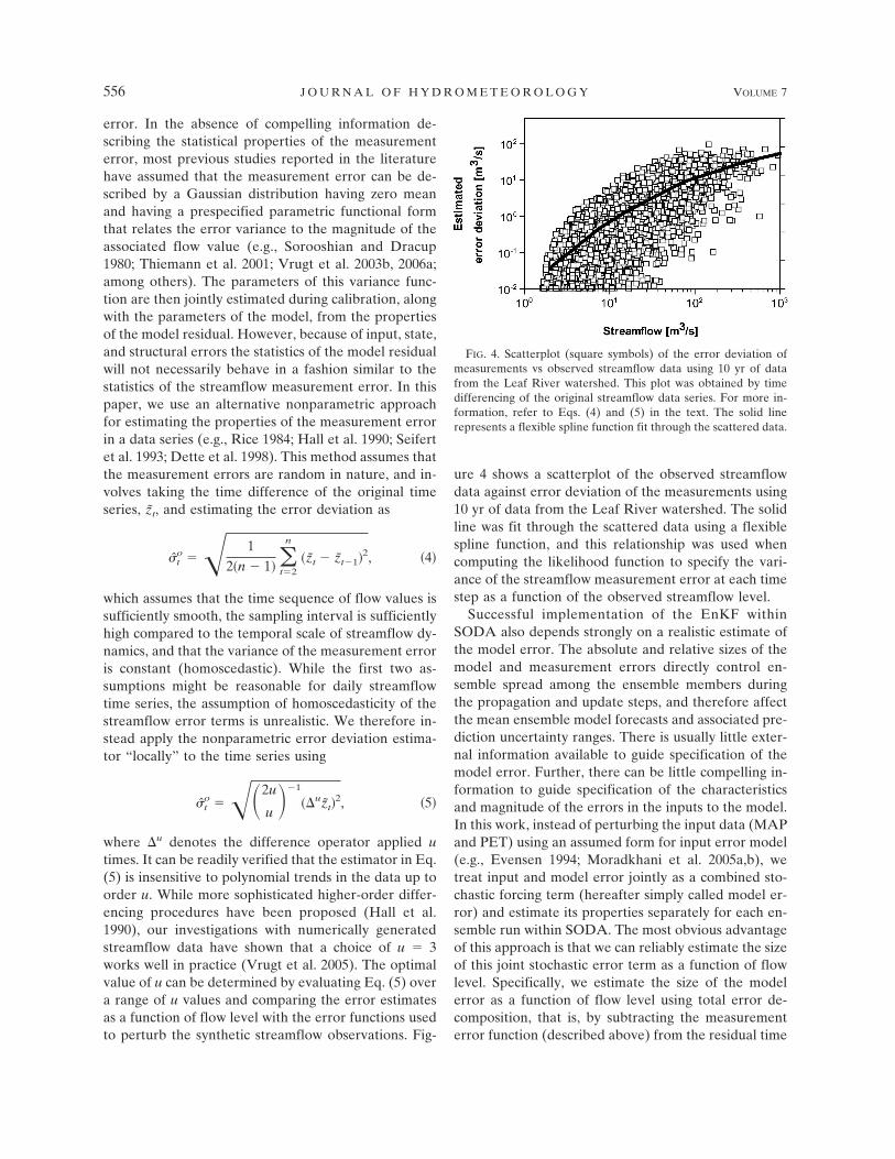
ure 4 shows a scatterplot of the observed streamflowdata against error deviation of the measurements using10 yr of data from the Leaf River watershed. The solidline was fit through the scattered data using a flexiblespline function, and this relationship was used whencomputing the likelihood function to specify the vari-ance of the streamflow measurement error at each timestep as a function of the observed streamflow level.

Successful implementation of the EnKF withinSODA also depends strongly on a realistic estimate ofthe model error. The absolute and relative sizes of themodel and measurement errors directly control en-semble spread among the ensemble members duringthe propagation and update steps, and therefore affectthe mean ensemble model forecasts and associated pre-diction uncertainty ranges. There is usually little exter-nal information available to guide specification of themodel error. Further, there can be little compelling in-formation to guide specification of the characteristicsand magnitude of the errors in the inputs to the model.In this work, instead of perturbing the input data (MAPand PET) using an assumed form for input error model(e.g., Evensen 1994; Moradkhani et al. 2005a,b), wetreat input and model error jointly as a combined sto-chastic forcing term (hereafter simply called model er-ror) and estimate its properties separately for each en-semble run within SODA. The most obvious advantageof this approach is that we can reliably estimate the sizeof this joint stochastic error term as a function of flowlevel. Specifically, we estimate the size of the modelerror as a function of flow level using total error de-composition, that is, by subtracting the measurementerror function (described above) from the residual time

FIG. 4. Scatterplot (square symbols) of the error deviation ofmeasurements vs observed streamflow data using 10 yr of datafrom the Leaf River watershed. This plot was obtained by timedifferencing of the original streamflow data series. For more in-formation, refer to Eqs. (4) and (5) in the text. The solid linerepresents a flexible spline function fit through the scattered data.


series obtained each time the SAC-SMA model isevaluated against an observed time series of data. Themodel error variance is, therefore, both dependent onflow level and conditional (as it should be) on the spe-cific parameter set used for each ensemble run.

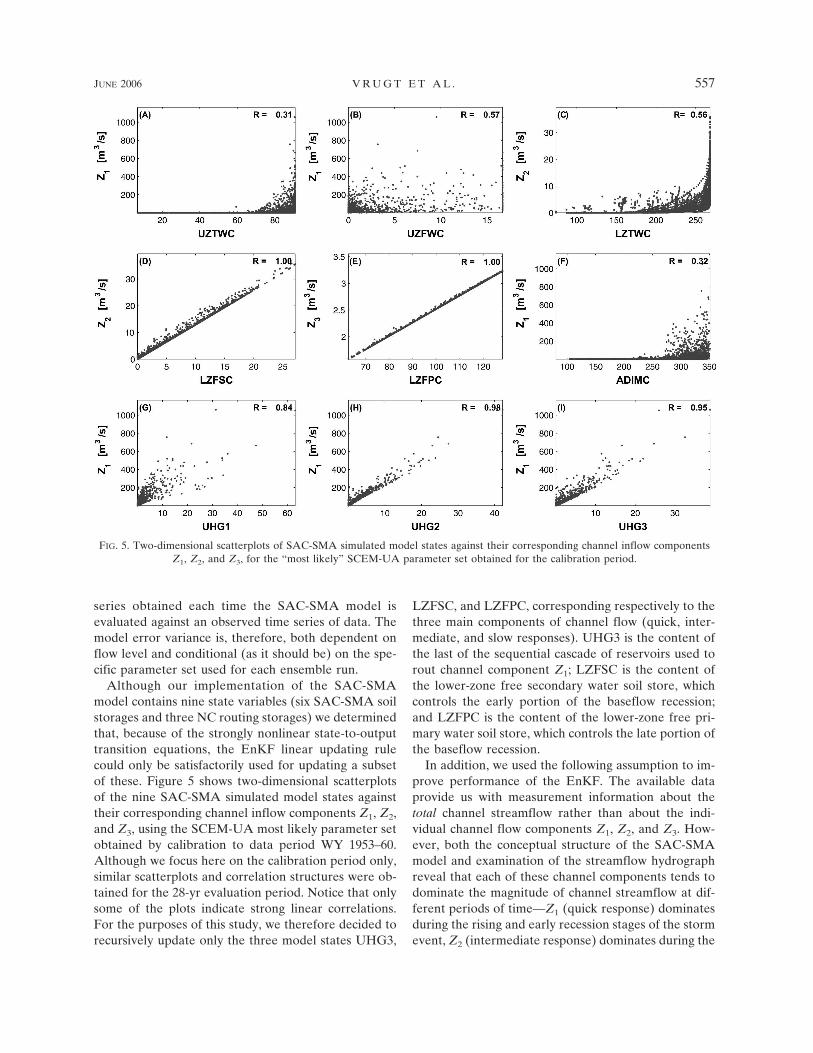
Although our implementation of the SAC-SMAmodel contains nine state variables (six SAC-SMA soilstorages and three NC routing storages) we determinedthat, because of the strongly nonlinear state-to-outputtransition equations, the EnKF linear updating rulecould only be satisfactorily used for updating a subsetof these. Figure 5 shows two-dimensional scatterplotsof the nine SAC-SMA simulated model states againsttheir corresponding channel inflow components Z1, Z2,and Z3, using the SCEM-UA most likely parameter setobtained by calibration to data period WY 1953–60.Although we focus here on the calibration period only,similar scatterplots and correlation structures were ob-tained for the 28-yr evaluation period. Notice that onlysome of the plots indicate strong linear correlations.For the purposes of this study, we therefore decided torecursively update only the three model states UHG3,

LZFSC, and LZFPC, corresponding respectively to thethree main components of channel flow (quick, inter-mediate, and slow responses). UHG3 is the content ofthe last of the sequential cascade of reservoirs used torout channel component Z1; LZFSC is the content ofthe lower-zone free secondary water soil store, whichcontrols the early portion of the baseflow recession;and LZFPC is the content of the lower-zone free pri-mary water soil store, which controls the late portion ofthe baseflow recession.

In addition, we used the following assumption to im-prove performance of the EnKF. The available dataprovide us with measurement information about thetotal channel streamflow rather than about the indi-vidual channel flow components Z1, Z2, and Z3. How-ever, both the conceptual structure of the SAC-SMAmodel and examination of the streamflow hydrographreveal that each of these channel components tends todominate the magnitude of channel streamflow at dif-ferent periods of time—Z1 (quick response) dominatesduring the rising and early recession stages of the stormevent, Z2 (intermediate response) dominates during the

FIG. 5. Two-dimensional scatterplots of SAC-SMA simulated model states against their corresponding channel inflow componentsZ1, Z2, and Z3, for the “most likely” SCEM-UA parameter set obtained for the calibration period.

JUNE 2006 V R U G T E T A L . 557

later recession stages of the storm event, and Z3 (slowresponse) dominates during the interstorm baseflow re-cession periods. We therefore assumed that the simu-lated (i.e., model computed) estimates Z1(�), Z2(�), andZ3(�) provide reasonable estimates of the relative frac-tions of the total streamflow observation Z̃ comingfrom each of the three components of channel flow.Based on this assumption, the measurement operatorwas modified so that

Z̃i�� Zi��

Z1�� Z2�� Z3�� Z̃ for each i � �1, 2, 3�,

�6�

which, in effect, partitions the scalar streamflow mea-surement Z̃t at each time step into a vector of threevalues Z̃1, Z̃2, and Z̃3.

Finally, a number of experiments were conducted toevaluate sensitivity of filter and parameter estimationperformance to the number of state-vector ensemblesto be used in the EnKF implementation. Figure 6 showsa plot of the normalized rmse ratio (NRR) againstEnKF ensemble size for the SODA estimated best pa-rameter set for a given ensemble size. NRR is calcu-lated in two steps: first the ratio of the time-averagedrmse of the ensemble mean to the mean rmse of theensemble members is computed (Ra), following whichRa is divided by �((N � 1)/2N), where N denotes theensemble size (see Fig. 2) (see Anderson 2001; Morad-khani et al. 2005a). A value of NRR close to 1.0 isdesirable; NRR greater than 1.0 indicates that the en-semble has too little spread, whereas NRR � 1 indi-cates too much spread. Figure 6 shows that the cali-brated model gives an NRR value close to unity, indi-cating that the size of the ensemble is of the correct

order of magnitude and that ensemble sizes larger than50 do not provide improved results. An ensemble sizeof N � 50 was used for all the studies reported in thispaper. Note that NRR values nearly identical to unitywere obtained when the model parameters were al-lowed to vary within the bounds obtained using a clas-sical Bayesian SCEM-UA calibration.

6. Discussion of results

Results of the model calibration phase of this studyare shown in Figs. 7 to 9 using WY 1953 for illustration.In all cases where a streamflow hydrograph is shown,box plot symbols are used to denote the median, lower,and upper quartile values of the confidence intervalsfor the streamflow data. Figure 7a shows the bench-mark deterministic model case where the SAC-SMAmodel was calibrated in the conventional manner(which implicitly assumes an accurate model structure),without state-variable updating, using the method de-scribed in section 5 to specify variation of output mea-surement error variance with flow level and the SCEM-UA algorithm to estimate parameter uncertainty.While the model-simulated estimates of streamflowlook reasonable, the simulated 95% confidence inter-vals for streamflow (dark gray region; generated byprojecting parameter uncertainty into the output space)are clearly too narrow and do not include the data,indicating that the estimation procedure is placing toomuch confidence in the validity of the model. Figure 7bshows the stochastic model case where the SAC-SMAmodel was calibrated using SODA (with EnKF recur-sive state-variable updating applied to each parameterset). The simulated overall 95% confidence intervalsfor streamflow, representing both parameter uncer-

FIG. 6. NRR as a function of ensemble size for the “most likely” SODA parameter set derived forthe calibration period.


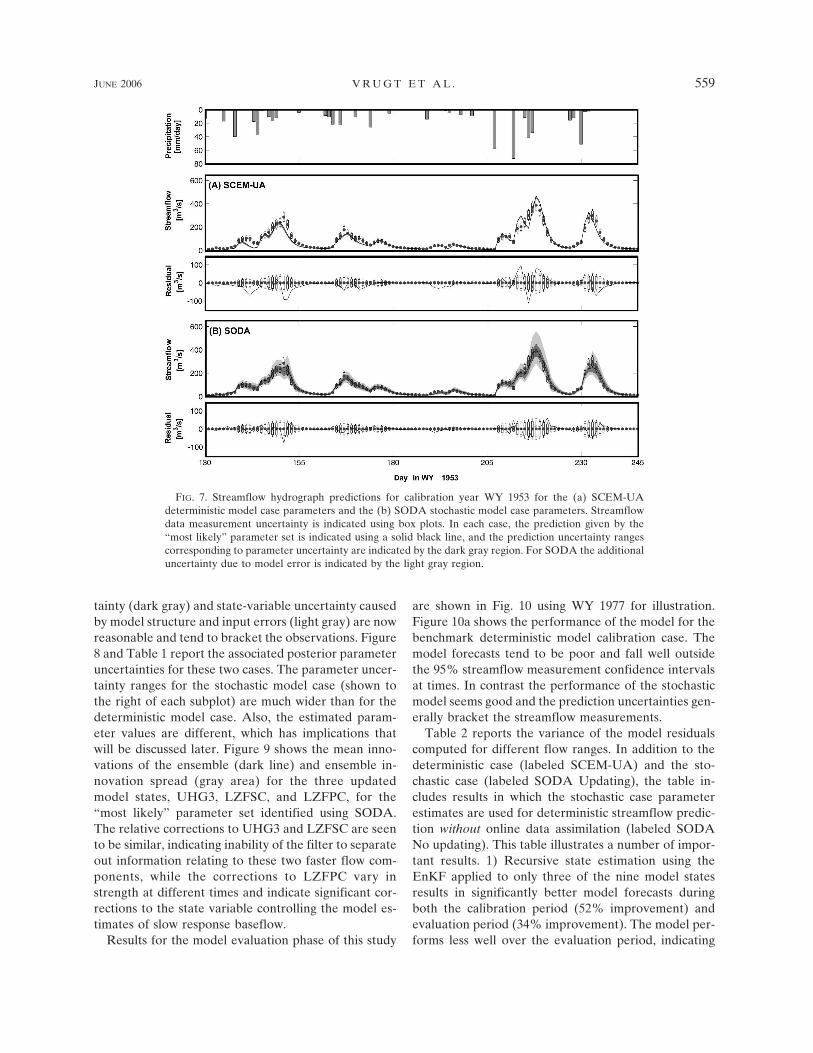
tainty (dark gray) and state-variable uncertainty causedby model structure and input errors (light gray) are nowreasonable and tend to bracket the observations. Figure8 and Table 1 report the associated posterior parameteruncertainties for these two cases. The parameter uncer-tainty ranges for the stochastic model case (shown tothe right of each subplot) are much wider than for thedeterministic model case. Also, the estimated param-eter values are different, which has implications thatwill be discussed later. Figure 9 shows the mean inno-vations of the ensemble (dark line) and ensemble in-novation spread (gray area) for the three updatedmodel states, UHG3, LZFSC, and LZFPC, for the“most likely” parameter set identified using SODA.The relative corrections to UHG3 and LZFSC are seento be similar, indicating inability of the filter to separateout information relating to these two faster flow com-ponents, while the corrections to LZFPC vary instrength at different times and indicate significant cor-rections to the state variable controlling the model es-timates of slow response baseflow.

Results for the model evaluation phase of this study

are shown in Fig. 10 using WY 1977 for illustration.Figure 10a shows the performance of the model for thebenchmark deterministic model calibration case. Themodel forecasts tend to be poor and fall well outsidethe 95% streamflow measurement confidence intervalsat times. In contrast the performance of the stochasticmodel seems good and the prediction uncertainties gen-erally bracket the streamflow measurements.

Table 2 reports the variance of the model residualscomputed for different flow ranges. In addition to thedeterministic case (labeled SCEM-UA) and the sto-chastic case (labeled SODA Updating), the table in-cludes results in which the stochastic case parameterestimates are used for deterministic streamflow predic-tion without online data assimilation (labeled SODANo updating). This table illustrates a number of impor-tant results. 1) Recursive state estimation using theEnKF applied to only three of the nine model statesresults in significantly better model forecasts duringboth the calibration period (52% improvement) andevaluation period (34% improvement). The model per-forms less well over the evaluation period, indicating

FIG. 7. Streamflow hydrograph predictions for calibration year WY 1953 for the (a) SCEM-UAdeterministic model case parameters and the (b) SODA stochastic model case parameters. Streamflowdata measurement uncertainty is indicated using box plots. In each case, the prediction given by the“most likely” parameter set is indicated using a solid black line, and the prediction uncertainty rangescorresponding to parameter uncertainty are indicated by the dark gray region. For SODA the additionaluncertainty due to model error is indicated by the light gray region.

JUNE 2006 V R U G T E T A L . 559

that the statistical properties of the rainfall–soil mois-ture–runoff transformation may be variable in time[i.e., the batch calibration assumption of time-invariantmodel structure and parameters may be incorrect—see

also Moradkhani et al. (2005a,b)]. 2) State estimationresults in much larger relative improvements to modelperformance at lower flows (�80% improvement) thanat high flows (�40% improvement for calibration/

FIG. 9. Mean ensemble innovations (dark line) for the LZFSC, LZFPC, and UHG3 states in theSAC-SMA model for calibration year WY 1953. Results correspond to the mode of the posteriordistribution identified using SODA. Dark gray ranges reflect uncertainty in the ensemble members.

FIG. 8. Posterior uncertainty ranges (box plots) for the (left) SCEM-UA deterministic model caseparameters and the (right) SODA stochastic model case parameters resulting from model calibrationusing the period WY 1953–60. The parameter uncertainties are scaled relative to their prior ranges toobtain normalized values.


�30% improvement for evaluation). This of coursecorrectly reflects the fact that the error variance of thestreamflow measurement data increases with stream-flow level. 3) The “most likely” parameter set esti-mated using SODA gives significantly better forecastperformance than the one estimated using SCEM-UAfor both the calibration and evaluation periods (SODANo updating case). This confirms our view (see Vrugt et

al. 2005) that proper acknowledgment of state-variableuncertainty (in addition to parameter uncertainty andoutput measurement error) can result in better esti-mates for the parameters (in the sense that they are lesscorrupted by system and other kinds of errors). Furthersupport for this claim is given in Clark and Vrugt(2006).

Figure 11 illustrates another test of model perfor-

TABLE 2. Summary statistic (rmse) for the one-day-ahead streamflow forecasts over the calibration and evaluation period using theSCEM-UA and SODA methods with and without recursive state updating. The error statistic is computed for different flow groups.

Calibration (WY 1953–60) Evaluation (WY 1961–88)

SCEM-UA

SODA

SCEM-UA

SODA

Flow group (m3 s�1) No updating Updating No updating Updating

0–5 3.36 1.73 0.55 3.42 1.44 0.655–10 8.22 3.91 1.76 7.02 3.36 1.7110–25 13.18 8.59 4.15 10.83 8.18 5.6825–50 19.74 15.54 9.19 22.78 15.67 10.9950–100 28.41 25.95 17.90 32.42 28.52 17.41100–250 69.89 58.29 33.03 53.83 53.06 43.12�250 129.81 121.41 78.47 128.63 111.45 102.29Overall 22.47 18.31 11.07 27.83 24.67 18.28

FIG. 10. Streamflow hydrograph predictions for evaluation year WY 1977 for the (a) SCEM-UAdeterministic model case parameters and the (b) SODA stochastic model case parameters. Streamflowdata measurement uncertainty is indicated using box plots. In each case, the prediction given by the“most likely” parameter set is indicated using a solid black line, and the prediction uncertainty rangescorresponding to parameter uncertainty are indicated by the dark gray region. For SODA the additionaluncertainty due to model error is indicated by the light gray region.

JUNE 2006 V R U G T E T A L . 561

mance and consistency. For each of the 36 water yearsused in this study (8 calibration plus 28 evaluation), theannual standard deviation of the one-day-aheadstreamflow forecast errors is plotted against the annualmean flow level for that year. Each box symbol indi-cates a calibration year and each “�” symbol indicatesan evaluation year. In all three cases the symbols ap-pear to fall approximately on a straight line indicatingthat calibration and evaluation period performance aremutually consistent. The slopes of the lines indicatethat forecast errors tend to be larger for wetter years(as reported also by Hsu et al. 2002). However, in thecase of SODA, the points are less scattered, the slope ofthe regression line is smaller and the intercept approxi-mately intersects the origin, indicating better and moreconsistent forecast performance. Further, a statisticalcheck of the autocorrelation functions of the residualsshowed that for both of the cases without state updatingthe forecast errors are strongly correlated. In contrast,the SODA forecast errors are essentially white (uncor-related), indicating that most of the bias in the one-day-ahead streamflow predictions is removed by the recur-sive state updating procedure.

Finally, it is worth mentioning that the performanceof the SAC-SMA model with recursive state estimationis very similar to that obtained for the same watershedby Hsu et al. (2002) using the deterministic SOLO ar-tificial neural network (ANN) approach having 1350parameters. The ANN results provide an indication ofthe limits to achievable forecasting performance for thiswatershed when using rainfall to predict streamflow.These results indicate that the SAC-SMA model is arelatively good representation of the rainfall–soil mois-ture–runoff transformation process for medium-sizedhumid watersheds such as the Leaf River. Taken to-gether with the parameter uncertainty results reported

in Fig. 8 and Table 1, they also further support our viewthat [contrary to suggestions by Jakeman and Horn-berger (1993)] the rainfall–runoff data can and do con-tain sufficient information for identifying models of thislevel of complexity (14� parameters and 9 state vari-ables).

7. Summary and conclusions

While conceptual watershed models are widely usedfor operational streamflow forecasting their stronglynonlinear structural equations (including threshold-type discontinuities) have historically posed a challengeto the application of computer-based systems’ methodsfor automated model identification, and parameter andstate estimation. Progress in stochastic global optimiza-tion methods has helped to diminish the difficulties as-sociated with parameter estimation. The recent devel-opment of ensemble-based techniques and filteringstrategies for sequential data assimilation now make itpossible (in principle) to implement techniques thatproperly account for data (input and output), state vari-able, parameter, and model structural uncertainties, al-though the details of how such implementation can beachieved are still an active area of research.

This paper has demonstrated the applicability of theSODA method for joint parameter–state estimationand operational ensemble streamflow forecasting usingthe SAC-SMA conceptual watershed model. SODAmerges the strengths of the ensemble Kalman filter forrecursive data assimilation to update model states, andthe shuffled complex evolution metropolis algorithmfor batch data assimilation to estimate time-invariantvalues for the model parameters. The algorithm wasimplemented using a LAM/MPI distributed processinginterface and Octave programming environment to

FIG. 11. Annual mean standard deviation of one-day-ahead streamflow forecast errors as function of meanannual flow level for the (a) SCEM-UA deterministic model case parameters, and the (b) SODA stochastic modelcase parameters without state updating and (c) with state updating. Calibration years are plotted using the boxsymbol, and evaluation years are plotted using the “�” symbol.


maximize computing efficiency, using 25 Pentium IV3.40-GHz processing nodes. Each stochastic joint cali-bration and ensemble state estimation run reported inthis paper using 50 000 SCEM-UA generated param-eter combinations required approximately 22 h of CPUtime.

The performance of the stochastic SODA method(using an ensemble size of 50) was compared to a con-ventional deterministic model calibration approach.The heteroscedastic error variance properties of thestreamflow measurement error were estimated fromthe data using a nonparametric approach and the het-eroscedastic error variance properties of the modelstructural error were estimated (for each parameterset) from the model residuals by subtraction. Becausethe EnKF uses a linear rule for state updating we de-cided to update only the three of the nine model statesthat showed strong cross covariances with the threemain components of channel flow (quick, intermediate,and slow responses). A simple but reasonable assump-tion was used to partition the scalar streamflow mea-surement at each time step into a vector correspondingto the three flow component values. The results may besummarized as follows:

1) The conventional deterministic approach gives nar-row estimates of streamflow uncertainty that do notinclude the data, indicating that the deterministicestimation procedure places too much confidence inthe validity of the model. In contrast, the stochasticSODA approach gives reasonable streamflow con-fidence intervals (neither too wide nor too narrow)that bracket the observations.

2) The parameter uncertainty ranges for the stochasticmodel case (SODA) are wider than for the deter-ministic model case (SCEM-UA) and lie in differentareas of the feasible parameter space. Further, theSODA “most likely” parameter set gives signifi-cantly better forecast performance (in nonupdating/simulation mode) than its SCEM-UA counterpart,indicating that proper treatment of state variable,parameter, and output measurement uncertaintiescan result in better (i.e., less biased) parameter esti-mates. This may increase the prospects for findinguseful regionalization relationships.

3) Although data assimilation via recursive state esti-mation was applied to only three of the nine modelstates, significant improvements in SAC-SMAmodel forecast performance were realized (on theorder of 30% to 50%).

4) State estimation resulted in larger relative improve-ments to model performance at lower flows than athigher flows, reflecting the fact that streamflow

measurement error variance increases with stream-flow level. Further, SODA forecast errors were es-sentially white (uncorrelated), indicating that mostof the bias in the one-day-ahead streamflow predic-tions was removed by recursive state updating.

5) The calibrated SAC-SMA model with stochasticstate-variable uncertainty propagation and updatingprovides streamflow forecast estimates that ap-proach the accuracy achievable using a sophisticated1350-parameter artificial neural network approach.These results suggest that the 16-parameter SAC-SMA model is a relatively good representation ofthe rainfall–soil moisture–runoff transformationprocess for medium-sized humid watersheds such asthe Leaf River.

On the negative side, we also found that the cali-brated model performs less well over the evaluationperiod, suggesting that the statistical properties of therainfall–soil moisture–runoff transformation may betime varying in a manner not adequately captured bythe SODA procedure. Part of this might be due to thefact that the evaluation period showed on average con-siderable higher flow values. In particular, the SCEM-UA batch calibration approach assumes that the systemstructure (as reflected in the structural equations andparameters) is time invariant and that the accuracy ofthe model (as reflected in the temporal trajectory ofmodel error bias) is stationary. Further, our approachdoes not yet properly account for input errors, particu-larly of the nonstationary kind arising from nondetec-tion of precipitation (caused by inadequate gauge den-sity and other factors). Nevertheless, the results of thisstudy indicate that the SODA method has the potentialfor ready implementation into operational forecastingprocedures, and the capability of providing improvedensemble streamflow forecasts without requiring sig-nificant modifications to operational model codes orsoftware. Research aimed at further improvements inalgorithm applicability, performance, and efficiency areongoing and will be reported in due course. As always,we invite dialogue with others interested in these top-ics. Software used in this and related work can be foundonline at www.science.uva.nl/ibed/cbpg/products and/or at www.sahra.arizona.edu/software.

Acknowledgments. The first author is supported bythe LANL Director’s Funded Postdoctoral program.In addition, we are grateful for partial support re-ceived from the National Weather Service (GrantsNA87WHO582 and NA07WH0144), the SAHRA Cen-ter for Sustainability of Semi arid Hydrology and Ri-parian Areas at the University of Arizona (NSF Grant

JUNE 2006 V R U G T E T A L . 563

EAR-9876800), and for computer support provided bythe SARA center for parallel computing at the Univer-sity of Amsterdam.

REFERENCES

Anderson, H., 2001: An ensemble adjustment filter for data as-similation. Mon. Wea. Rev., 129, 2884–2903.

Arulampalam, M. S., S. Maskell, N. Gordon, and T. Clapp, 2002:A tutorial on particle filters for online nonlinear/non-Gaussian Bayesian tracking. IEEE Trans. Signal Process., 50(2), 174–188.

Awwad, H. M., and J. B. Valdés, 1992: Adaptive parameter esti-mation for multi-site hydrologic forecasting. J. Hydraul. Eng.,118, 1201–1221.

——, ——, and P. J. Restrepo, 1994: Streamflow forecasting forHan River basin, Korea. J. Water Resour. Plann. Manage.,120, 651–673.

Beven, K. J., and A. M. Binley, 1992: The future of distributedmodels: Model calibration and predictive uncertainty. Hy-drol. Processes, 6, 279–298.

Box, G. E. P., and G. C. Tiao, 1973: Bayesian Inference in Statis-tical Analyses. Addison-Wesley-Longman, 585 pp.

Boyle, D. P., H. V. Gupta, and S. Sorooshian, 2000: Towards im-proved calibration of hydrologic models: Combining thestrengths of manual and automatic methods. Water Resour.Res., 36, 3663–3674.

——, ——, and ——, 2001: Towards improved streamflow fore-casts: The value of semi-distributed modeling. Water Resour.Res., 37, 2749–2759.

Bras, R. L., and P. Restrepo-Posada, 1980: Real time automaticparameter calibration in conceptual runoff forecasting mod-els. Proc. Third Int. Symp. on Stochastic Hydraulics, 61–70.

——, and I. Rodriguez-Iturbe, 1985: Random Functions and Hy-drology. Addison-Wesley, 545 pp.

Brazil, L. E., and M. D. Hudlow, 1981: Calibration proceduresused with the National Weather Service Forecast System.Water and Related Land Resources, Y. Y. Haimes and J. Kin-dler, Eds., Pergamon Press, 457–466.

Burnash, R. J. C., R. L. Ferral, and R. A. McGuire, 1973: A gen-eralized streamflow simulation system: Conceptual modelsfor digital computers. National Weather Service, NOAA, andthe State of California Department of Water ResourcesTech. Rep., Joint Federal–State River Forecast Center, Sac-ramento, CA, 68 pp.

Cañizares, R., H. Madsen, H. R. Jensen, and H. J. Vested, 2001:Developments in operational shelf sea modeling in Danishwaters. Estuarine Coastal Shelf Sci., 53, 595–605.

Clark, M. P., and J. A. Vrugt, 2006: Unraveling uncertainties inhydrologic model calibration: Addressing the problem ofcompensatory parameters. Geophys. Res. Lett., 33, L06406,doi:10.1029/2005GL025604.

Dette, H., A. Munk, and T. Wagner, 1998: Estimating the variancein nonparametric regression—What is a reasonable choice? J.Roy. Stat. Soc., 60B, 751–764.

Duan, Q., V. K. Gupta, and S. Sorooshian, 1992: Effective andefficient global optimization for conceptual rainfall-runoffmodels. Water Resour. Res., 28, 1015–1031.

——, S. Sorooshian, and V. K. Gupta, 1994: Optimal use of theSCE-UA global optimization method for calibrating water-shed models. J. Hydrol., 158, 265–284.

Eaton, J. W., 1998: Octave Version 1. Department of Chemical

Engineering, University of Wisconsin. [Available online athttp://www.octave.org.]

——, 2001: Octave: Past, Present and Future. Proc. Second Int.Workshop on Distributed Statistical Computing, Vienna, Aus-tria, Technical University of Vienna, 1–17.

Evensen, G., 1992: Using the extended Kalman filter with a multi-layer quasi-geostrophic ocean model. J. Geophys. Res., 97(C11), 17 905–17 924.

——, 1994: Sequential data assimilation with a nonlinear quasi-geostrophic model using Monte Carlo methods to forecasterror statistics. J. Geophys. Res., 99, 10 143–10 162.

Fernández, J., A. Cañas, A. F. Díaz, J. González, J. Ortega, and A.Prieto, 2003: Performance of message-passing MATLABtoolboxes. Lect. Notes Comput. Sci., 2565, 228–241.

——, M. Anguita, S. Mota, A. Cañas, E. Ortigosa, and F. J. Rojas,2004: MPI toolbox for Octave. Proc. Sixth Int. Conf. on HighPerformance Computing for Computational Science, Valen-cia, Spain, Polytechnic University of Valencia, 1–6.

Freer, J., K. J. Beven, and B. Ambroise, 1996: Bayesian estimationof uncertainty in runoff prediction and the value of data: Anapplication of the GLUE approach. Water Resour. Res., 32,2161–2173.

Georgakakos, H., and J. A. Sperflage, 1995: Hydrologic forecastsystem-HFS: A user’s manual. HRC Tech. Note 1, Hydro-logic Research Center, San Diego, CA, 17 pp.

——, H. Rajaram, and S. G. Li, 1988: On improved operationalhydrologic forecasting of streamflows. Iowa Institute of Hy-draulic Research Rep. 325, 162 pp.

Gordon, N. D., D. Salmond, and A. F. M. Smith, 1993: Novelapproach to nonlinear and non-Gaussian Bayesian state es-timation. Proc. Inst. Electr. Eng., Part F, 140, 107–113.

Gupta, H. V., S. Sorooshian, and P. O. Yapo, 1998: Towards im-proved calibration of hydrologic models: Multiple and non-commensurable measures of information. Water Resour. Res.,34, 751–763.

——, ——, T. S. Hogue, and D. P. Boyle, 2003: Advances in au-tomatic calibration of watershed models. Calibration of Wa-tershed Models, Q. Duan et al., Eds., Water Science Appli-cations Series, Vol. 6, Amer. Geophys. Union, 113–124.

Gupta, V. K., and S. Sorooshian, 1985: The relationship betweendata and the precision of estimated parameters. J. Hydrol.,81, 57–77.

Hall, P., J. W. Kay, and D. M. Titterington, 1990: Asymptoticallyoptimal difference-based estimation of variance in nonpara-metric regression. Biometrika, 77, 521–528.

Hogue, T. S., S. Sorooshian, H. V. Gupta, A. Holz, and D. Braatz,2000: A multi-step automatic calibration scheme (MACS) forriver forecasting models. J. Hydrometeor., 1, 524–542.

——, H. V. Gupta, and S. Sorooshian, 2005: A “user-friendly”approach to parameter estimation in hydrologic models. J.Hydrol., 320, 202–217.

Hsu, K., H. V. Gupta, X. Gao, S. Sorooshian, and B. Imam, 2002:Self-organizing linear output map (SOLO): An artificial neu-ral network suitable for hydrologic modeling and analysis.Water Resour. Res., 38, 1302, doi:10.1029/2001WR000795.

Jakeman, A., and G. M. Hornberger, 1993: How much complexityis warranted in a rainfall-runoff model? Water Resour. Res.,29, 2637–2649.

Kalman, R., 1960: New approach to linear filtering and predictionproblems. J. Basic Eng., 82D, 35–45.

Kavetski, D., S. W. Franks, and G. Kuczera, 2003: Confrontinginput uncertainty in environmental modeling. Calibration of


Watershed Models, Q. Duan et al., Eds., Water Science Ap-plications Series, Vol. 6, Amer. Geophys. Union, 49–68.

Keesman, K. J., 1990: Set theoretic parameter estimation usingrandom scanning and principal component analysis. Math.Comput. Simul., 32, 535–543.

Kitanidis, P. K., and R. L. Bras, 1980a: Real time forecasting witha conceptual hydrologic model, 1, Analysis of uncertainty.Water Resour. Res., 16, 1025–1033.

——, and ——, 1980b: Real time forecasting with a conceptualhydrologic model, 2, Applications and results. Water Resour.Res., 16, 1034–1044.

Klepper, O., H. Scholten, and J. P. G. van de Kamer, 1991: Pre-diction uncertainty in an ecological model of the Ooster-schelde Estuary. J. Forecasting, 10, 191–209.

Kuczera, G., 1983a: Improved parameter inference in catchmentmodels: 1. Evaluating parameter uncertainty. Water Resour.Res., 19, 1151–1162.

——, 1983b: Improved parameter inference in catchment models:2. Combining different kinds of hydrologic data and testingtheir compatibility. Water Resour. Res., 19, 1163–1172.

——, 1997: Efficient subspace probabilistic parameter optimiza-tion for catchment models. Water Resour. Res., 33, 177–185.

Madsen, H., 2000: Automatic calibration of a conceptual rainfall-runoff model using multiple objectives. J. Hydrol., 235, 276–288.

——, and C. Skotner, 2005: Adaptive state-updating in real-timeriver flow forecasting—A combined filtering and error fore-casting procedure. J. Hydrol., 308, 302–312.

Miller, R. N., M. Ghil, and F. Ghautiez, 1994: Advanced dataassimilation in strongly nonlinear dynamical systems. J. At-mos. Sci., 51, 1037–1055.

Misirli, F., 2003: Improving efficiency and effectiveness of Bayes-ian recursive parameter estimation for hydrologic models.Ph.D. dissertation, The University of Arizona.

Moradkhani, H., S. Sorooshian, H. V. Gupta, and P. R. Hauser,2005a: Dual state–parameter estimation of hydrological mod-els using ensemble Kalman filter. Adv. Water Res., 28, 135–147.

——, K. Hsu, H. V. Gupta, and S. Sorooshian, 2005b: Uncertaintyassessment of hydrologic model states and parameters: Se-quential data assimilation using the particle filter. Water Re-sour. Res., 41, W05012, doi:10.1029/2004WR003604.

Refsgaard, J. C., 1998: Validation and intercomparison of differ-ent updating procedures for real-time forecasting. Nord. Hy-drol., 28, 65–84.

Reichle, R. H., D. Entekhabi, and D. B. McLaughlin, 2001:Downscaling radio brightness measurements for soil mois-ture estimation: A four dimensional variational data assimi-lation approach. Water Resour. Res., 37, 2353–2364.

Rice, J., 1984: Bandwidth choice for nonparametric kernel regres-sion. Ann. Stat., 12, 1215–1230.

Seifert, B., T. Gasser, and A. Wolf, 1993: Nonparametric estima-tion of residual variance revisited. Biometrika, 80, 373–383.

Seo, D. J., V. Koren, and N. Cajina, 2003: Real-time variationalassimilation of hydrologic and hydrometeorological data intooperational hydrologic forecasting. J. Hydrometeor., 4, 627–641.

Sorooshian, S., and J. A. Dracup, 1980: Stochastic parameter es-timation procedures for hydrologic rainfall-runoff models:Correlated and heteroscedastic error cases. Water Resour.Res., 16, 430–442.

——, and V. K. Gupta, 1983: Automatic calibration of conceptualrainfall-runoff models: The question of parameter observ-ability and uniqueness. Water Resour. Res., 19, 260–268.

——, Q. Duan, and V. K. Gupta, 1993: Calibration of rainfall-runoff models: Application of global optimization to the Sac-ramento soil moisture accounting model. Water Resour. Res.,29, 1185–1194.

Thiemann, M., M. W. Trosset, H. V. Gupta, and S. Sorooshian,2001: Bayesian recursive parameter estimation for hydrologicmodels. Water Resour. Res., 37, 2521–2535.

Todini, E., A. Szollosi-Nagy, and E. F. Wood, 1976: Adaptivestate-parameter estimation algorithm for real time hydrologicforecasting: A case study. Proc. IIASA/WMO Workshop onthe Recent Developments in Real Time Forecasting/Controlof Water Resources Systems, Laxenburg, Austria, IIASA–Laxenburg.

van Straten, G., and K. J. Keesman, 1991: Uncertainty propaga-tion and speculation in projective forecasts of environmentalchange: A lake eutrophication example. J. Forecasting, 10,163–190.

Vrugt, J. A., W. Bouten, H. V. Gupta, and S. Sorooshian, 2002:Toward improved identifiability of hydrologic model param-eters: The information content of experimental data. WaterResour. Res., 38, 1312, doi:10.1029/2001WR001118.

——, H. V. Gupta, L. Bastidas, W. Bouten, and S. Sorooshian,2003a: Effective and efficient algorithm for multiobjectiveoptimization of hydrologic models. Water Resour. Res., 39,1214, doi:10.1029/2002WR001746.

——, ——, W. Bouten, and S. Sorooshian, 2003b: A shuffled com-plex evolution metropolis algorithm for optimization and un-certainty assessment of hydrologic model parameters. WaterResour. Res., 39, 1201, doi:10.1029/2002WR001642.

——, C. G. H. Diks, H. V. Gupta, W. Bouten, and J. M. Ver-straten, 2005: Improved treatment of uncertainty in hydro-logic modeling: Combining the strengths of global optimiza-tion and data assimilation. Water Resour. Res., 41, W01017,doi:10.1029/2004WR003059.

——, H. V. Gupta, S. C. Dekker, S. Sorooshian, T. Wagener, andW. Bouten, 2006a: Application of stochastic parameter opti-mization to the Sacramento Soil Moisture Accounting model.J. Hydrol., in press.

——, B. Ó. Nualláin, B. A. Robinson, W. Bouten, S. C. Dekker,and P. M. A. Sloot, 2006b: Application of parallel computingto stochastic parameter estimation in environmental models.Comput. Geosci., in press.

Wagener, T., N. McIntyre, M. J. Lees, H. S. Wheater, and H. V.Gupta, 2003: Towards reduced uncertainty in conceptualrainfall-runoff modeling: Dynamic identifiability analysis.Hydrol. Processes, 17, 455–476.

Wood, E. F., and P. E. O’Connell, 1985: Real-time forecasting.Hydrological Forecasting, M. G. Anderson and T. P. Burt,Eds., John Wiley and Sons.

Yapo, P., H. V. Gupta, and S. Sorooshian, 1996: Automatic cali-bration of conceptual rainfall-runoff models: Sensitivity tocalibration data. J. Hydrol., 181, 23–48.

Young, P. C., 2001: Data-based mechanistic modeling and valida-tion of rainfall-flow processes. Model Validation, M. G.Anderson and P. G. Bates, Eds., John Wiley and Sons, 117–161.

——, 2002: Advances in real-time flood forecasting. Philos. Trans.Roy. Soc. London, 360, 1433–1450.

JUNE 2006 V R U G T E T A L . 565

real-time data assimilation for operational ensemble...

Documents