REAL MATHEMATICAL ANALYSIS

Lectures by Niranjan Balachandran, IIT Bombay.

Contents

1 Preliminaries: The Real Line 51.1 Relations . . . . . . . . . . . . . . . . . . . . . . . . . . . . . . . . . . . . 51.2 Natural Numbers . . . . . . . . . . . . . . . . . . . . . . . . . . . . . . . 6

1.2.1 Axioms for Natural Numbers N . . . . . . . . . . . . . . . . . . . 61.2.2 Addition and Multiplication . . . . . . . . . . . . . . . . . . . . . 71.2.3 Order on N . . . . . . . . . . . . . . . . . . . . . . . . . . . . . . 81.2.4 The Well Ordering Principle, and the Euclidean Algorithm . . . . 91.2.5 Prime Numbers . . . . . . . . . . . . . . . . . . . . . . . . . . . . 10

1.3 Integers . . . . . . . . . . . . . . . . . . . . . . . . . . . . . . . . . . . . 111.3.1 Addition on Z . . . . . . . . . . . . . . . . . . . . . . . . . . . . . 121.3.2 Multiplication on Z . . . . . . . . . . . . . . . . . . . . . . . . . . 131.3.3 Subtraction . . . . . . . . . . . . . . . . . . . . . . . . . . . . . . 131.3.4 Order on Z . . . . . . . . . . . . . . . . . . . . . . . . . . . . . . 15

1.4 Rational Numbers . . . . . . . . . . . . . . . . . . . . . . . . . . . . . . . 171.4.1 Addition and Multiplication on Q . . . . . . . . . . . . . . . . . . 181.4.2 Order on Q . . . . . . . . . . . . . . . . . . . . . . . . . . . . . . 201.4.3 Q misses some ‘numbers’ . . . . . . . . . . . . . . . . . . . . . . 21

1.5 Real Numbers . . . . . . . . . . . . . . . . . . . . . . . . . . . . . . . . . 231.5.1 Addition and Multiplication on R . . . . . . . . . . . . . . . . . . 241.5.2 Another description for Real Numbers . . . . . . . . . . . . . . . 271.5.3 Archimedian Property of R . . . . . . . . . . . . . . . . . . . . . 28

1

1.6 Cardinality . . . . . . . . . . . . . . . . . . . . . . . . . . . . . . . . . . 321.7 The Complex Numbers . . . . . . . . . . . . . . . . . . . . . . . . . . . . 38

2 Basic Topology 392.1 Metric Spaces . . . . . . . . . . . . . . . . . . . . . . . . . . . . . . . . . 392.2 Subsequences . . . . . . . . . . . . . . . . . . . . . . . . . . . . . . . . . 452.3 Continuity . . . . . . . . . . . . . . . . . . . . . . . . . . . . . . . . . . . 472.4 Compactness . . . . . . . . . . . . . . . . . . . . . . . . . . . . . . . . . 482.5 Induced Topology on Subsets of R . . . . . . . . . . . . . . . . . . . . . . 522.6 Extending from the Reals to arbitrary Metric spaces . . . . . . . . . . . . 542.7 Connectedness . . . . . . . . . . . . . . . . . . . . . . . . . . . . . . . . . 55

2.7.1 A Weird Closed Set in R: . . . . . . . . . . . . . . . . . . . . . . 572.7.2 Pathological Examples: . . . . . . . . . . . . . . . . . . . . . . . . 58

2.8 Another Construction of R from Q . . . . . . . . . . . . . . . . . . . . . 602.9 Returning to the Cantor Set . . . . . . . . . . . . . . . . . . . . . . . . . 64

3 Differentiation 653.1 Differentiation of Real Valued Functions . . . . . . . . . . . . . . . . . . 653.2 The Mean Value Theorems and Consequences . . . . . . . . . . . . . . . 69

3.2.1 A Theorem of Darboux . . . . . . . . . . . . . . . . . . . . . . . . 703.2.2 The L’Hopital Rule . . . . . . . . . . . . . . . . . . . . . . . . . . 71

3.3 Series . . . . . . . . . . . . . . . . . . . . . . . . . . . . . . . . . . . . . . 733.3.1 Power Series . . . . . . . . . . . . . . . . . . . . . . . . . . . . . . 783.3.2 Taylor Series and Taylor Approximation . . . . . . . . . . . . . . 80

3.4 Uniform Convergence . . . . . . . . . . . . . . . . . . . . . . . . . . . . . 823.4.1 The Metric Space (C[0, 1], d) . . . . . . . . . . . . . . . . . . . . . 833.4.2 Theorems of Weierstrass . . . . . . . . . . . . . . . . . . . . . . . 853.4.3 Baire Category Theorem . . . . . . . . . . . . . . . . . . . . . . . 90

4 Riemann Integration 934.1 Integrals according to Riemann and Darboux . . . . . . . . . . . . . . . . 934.2 Measure Zero sets and Riemann Integrability . . . . . . . . . . . . . . . . 964.3 Consequences of the Riemann-Lebesgue Theorem . . . . . . . . . . . . . 1004.4 Antiderivatives and some ‘well known’ Integral Calculus techniques . . . 1024.5 The Integral Test . . . . . . . . . . . . . . . . . . . . . . . . . . . . . . . 1074.6 Weak version of Stirling’s formula for n! . . . . . . . . . . . . . . . . . . 1084.7 Convergence of sequences of functions and Integrals . . . . . . . . . . . . 110

5 Measures of sets and a peek into Lebesgue Integration 1135.1 Measure for subsets of R . . . . . . . . . . . . . . . . . . . . . . . . . . . 1135.2 Sigma Algebras and the Borel Sigma Field . . . . . . . . . . . . . . . . . 1245.3 Lebesgue Integration . . . . . . . . . . . . . . . . . . . . . . . . . . . . . 1245.4 Lebesgue’s Monotone Convergence Theorem . . . . . . . . . . . . . . . . 133

2

Preface

Real Analysis is all about formalizing and making precise, a good deal of the intuitionthat resulted in the basic results in Calculus. As it turns out, the intuition is spot on, inseveral instances, but in some cases (and this is really why Real Analysis is important atall), our sense of intuition is so far from reality, that one needs some kind of guarantee,or validation to our heuristic arguments.

I thank all my students of this course who very actively and enthusiastically acted asscribes for the lectures for this course.

3

1 Preliminaries: The Real Line

As mentioned in the preface, in order to formalize the results one has studied in a firstCalculus course, one needs to start at the very beginning, in order to ensure that thereis no inconsistency in our settings. And we shall begin at the very beginning - with theNatural numbers.

It may be a bit difficult to formally define what the natural numbers actually are. But,we shall avoid doing this, by making our approach axiomatic. The more important thingis to ensure that the axioms are no contradictory. As it turns out, very basic axioms aboutthe natural numbers are sufficient to set up our understanding of the natural numbers ina wholesome manner.

1.1 Relations

Definition 1 Suppose S is a set,then the Relation R on S is defined as a subset of

S × S := (s1, s2)|s1, s2 ∈ S

If (s1, s2) ∈ R we denote it as s1 ∼ s2.

Definition 2 1. A relation R is Reflexive if a ∼ a , ∀ a ∈ S

2. A relation R is Symmetric if a ∼ b ⇒ a ∼ b , ∀ a, b ∈ S

3. A relation R is Transitive if a ∼ b , b ∼ c ⇒ a ∼ c ,∀ a, b, c ∈ S

Definition 3 (Equivalence Relation)A relation is an Equivalence relation iff it is Reflexive, Symmetric and Transitive.

Proposition 1 Suppose ∼ is an equivalence relation defined on a set S, then ∼ inducesa partition on S. Conversely, for any partition Π = Sαα∈λ of the set S, there is anequivalence relation ∼Π which induces partition Π on S.

5

Proof: Given ∼, an equivalence relation, for each a ∈ S ,define

Sa = b ∈ S|b ∼ a

Claim 1 Saa∈S is a partition of S.

Let a 6= b, where a, b ∈ S. Consider Sa ∩ Sb. Suppose Sa ∩ Sb 6= Φ. We shall show thatSa ⊆ (Sa ∩ Sb). Similarly, Sb ⊆ (Sa ∩ Sb) and these will prove that Sa = Sb = (Sa ∩ Sb).

Since Sa ∩ Sb 6= Φ, there exists some c ∈ (Sa ∩ Sb). Let x ∈ Sa. Then we have x ∼ a.However, since c ∈ Sa, we have c ∼ a⇒ a ∼ c , by symmetry. Therefore, by transitivity,x ∼ c. And since c ∼ b, we also get x ∼ b ⇒ x ∈ Sb. Now that x ∈ Sa and x ∈ Sb,x ∈ (Sa∩Sb). Since this is true for any x ∈ Sa, we have Sa ⊆ (Sa∩Sb). Similarly, we canshow that Sb ⊆ (Sa∩Sb). Thus, Sa = Sb = (Sa∩Sb) which is a partition of S induced by∼.

Converse: Given Π = Sαα∈λ, a partition of S, we define a relation ∼Π as follows:

a ∼Π b if ∃ α ∈ λ such that a, b ∈ SαNow, we prove that it is an equivalence relation on S.

Reflexivity: (a ∼Π a) ∀a ∈ S as it is in the same partition as itself.Symmetry: a ∼Π b ⇒ a is in the same partition as b ⇒ b is in the same partition asa⇒ b ∼Π aTransitivity: a ∼Π b,⇒ a, b ∈ Sα and b ∼Π c,⇒ b, c ∈ Sβ. But since S has beenpartitioned by Π and b belongs to both Sα and Sβ, we must have Sα = Sβ. Hence a andc belong to Sα and are related under ∼Π, thus proving the transitivity.These three properties put together make ∼Π an equivalence relation defined on S. ♣

1.2 Natural Numbers

1.2.1 Axioms for Natural Numbers N1. 0 ∈ N.

2. For each n ∈ N there is a unique successor for n, denoted by n+ 1.

3. If S ⊆ N,satisfying

• 0 ∈ N.

• n ∈ N⇒ n+ 1 ∈ N.

then S = N. This is referred to as The Principle of Mathematical Induction.

4. For each n ∈ N \0, there exists a unique m ∈ N such that m+ 1 = n.

6

1.2.2 Addition and Multiplication

We can define two operations on N called ‘addition, multiplication’ that satisfies thefollowing. We skip the proofs.

Theorem 1 Given m,n ∈ N ,there exists a binary operation ’+’ on N satisfying:

1. 0 + n = n, ∀ n ∈ N.

2. m+ n = n+m, ∀m,n ∈ N. (Commutative Property)

3. m+ (n+ p) = (m+ n) + p, ∀m,n, p ∈ N. (Associative Property)

♣

Theorem 2 Given m,n, p ∈ N ,there exists a binary operation ’.’ on N satisfying:

1. 1.n = n ∀n ∈ N.

2. m.n = n.m, ∀m,n ∈ N. (Commutative Property)

3. m.(n.p) = (m.n).p, ∀m,n, p ∈ N. (Associative Property)

4. m.(n+ p) = m.n+m.p, ∀m,n, p ∈ N. (Distributive Property)

♣

Example 1 Prove that 2+2=4.

Proof:

2 + 2 =2 + (1 + 1) . . . (since 2 is successor of 1),

=(2 + 1) + 1 . . . (Associative property),

=3 + 1 . . . (3 is successor of 2),

=4 . . . (4 is successor of 3).

♣

7

1.2.3 Order on NDefinition 4 We say a > b, if

1. a = b+ c for some c ∈ N,

2. a 6= b.

The following theorem follows from the definition of order. The proof is again skipped.

Theorem 3 ′ >′ on N satisfies

1. a > b⇒ a+ c > b+ c ∀ c ∈ Z.

2. a > b and c > 0⇒ ac > bc.

3. a > b, b > c⇒ a > c. (Transitivity)

4. Given a, b ∈ N, precisely one of a > b or b > a or a = b is satisfied.

5. 0 < 1 < 2 < 3 < · · ·

♣

Lemma 1 If c, d ∈ N, and c+ d = 0 , then c = d = 0.

Proof: Suppose c 6= 0. Then,

c =c′ + 1

c+ d =(c′ + 1) + d

=(c′ + d) + 1

=0

So, it follows that 0 is the successor of c′ + d, which is a contradiction to the fact that 0has no predecessor in N. Hence proved. ♣

Remark 1 If x = x+ y, then y = 0.

Note 1 Suppose a, b ∈ N and suppose a > b, can we have b > a too?

If yes, then

a > b⇒ a = b+ c

and

b > a⇒ b = a+ d

8

where c, d ∈ N and c, d 6= 0⇒ (a+ b) = (a+ b) + (c+ d). From earlier remark, we havec = d = 0 which shows that only one of the above two is possible, else they are equal.

Remark 2 We have already seen that 0 < 1 < 2 < 3 . . . . In particular, we have:For any a ∈ N, a < (a+ 1) + b for any b ∈ N, b > 0.

1.2.4 The Well Ordering Principle, and the Euclidean Algorithm

We start with an equivalent formulation to the principle of Induction, known as thePrinciple of Complete Induction.

1. 0 ∈ S.

2. 0, 1, 2, ..., n ⊆ S ⇒ n+ 1 ∈ S.

Then S = N. The proof is a simple consequence of the principle of Mathematical Induc-tion. We skip the proof.

Proposition 2 The Well Ordering Principle (WOP): Every non empty subsetS ⊂ N contains a least element, i.e., there exists s ∈ S such that s < s′ for all s′ ∈S, s′ 6= s.

Proof: For natural numbers a < b, we shall denote by [a, b] the set a, a+1, . . . , b−1, b.

Let ∅ ( S ⊂ N. We need to show that S has a minimal element.Suppose S has no minimal element. Let P (n) be the propositional function: n /∈ S.

We have two cases:

Case 1: 0 ∈ S. Since 0 is the least element of N, it is also the minimal element of Swhich is a contradiction.

Case 2: 0 /∈ S so P (0) holds. Suppose P (j) holds for 0 ≤ j ≤ k, i.e., suppose for allj ∈ [0, k] : j /∈ S.

If k + 1 ∈ S then k + 1 would be the minimal element of S. So k + 1 /∈ S and soP (k + 1) also holds. Thus we have proven the following.

1. P (0) holds.

2. For all j ∈ [0, k] : P (j) holds) ⇒ P (k + 1) holds.

So by the principle of complete induction P (n) holds for all n ∈ N. But this means Sis empty which is a contradiction. ♣

A simple consequence is the following:

9

Theorem 4 Euclidean division and the Euclidean algorithm: Given positiveintegers m,n there exist unique non-negative integers q, r such that m = qn+r, 0 ≤ r < n.We describe this by saying that the Euclidean algorithm when applied to the ordered pair(m,n) gives a quotient of q and remainder r.

Proof: Define S = m − kn | k ∈ N0,m − kn > 0. Now, S ⊂ N0 and S 6= Φ asm− 0.n = m ∈ S. By WOP, S has a least element; call it r = m− qn. We claim

1. 0 ≤ r < n.

2. q, r as determined above, are unique.

To prove this claim, note that by definition of S, r ≥ 0. Indeed, suppose otherwise. Thenm − (q + 1)n = m − qn − n = r − n ≥ 0, and this implies m − (q + 1)n ∈ S. Alsom− (q + 1)n = r − n < r as n > 0. Hence, r is not the least element of S, and this is acontradiction. This proves the first part.

To prove the second, again, suppose otherwise. Let m = q1n + r1 and m = q2n + r2

be two such representations and WLOG, let r2 > r1.Equating the RHS of the above equations and simplifying,(q1 − q2)n = r2 − r1,⇒ r2 − r1 is a multiple of n. But since, r1, r2 < n, r2 − r1 < n, the only possibility isr2 − r1 = 0. which implies that r1 = r2 and it follows that q1 = q2 and this proves thesecond claim as well.

Thus, r, q are unique integers satisfying r ∈ [0, n) and m = qn+ r. ♣

A very important consequence of the Euclidean algorithm is the following. For natu-ral numbers a, b we say that n divides m if the corresponding value of r in the Euclideanalgorithm above equals 0. For natural numbers a, b we say that d is the greatest com-mon divisor (and denoted (a, b)) of a, b if d divides a, b and for any d′ that divides botha, b we also have d divides d′. A very useful consequence of the Euclidean algorithm isthis: Given m,n, r as in the theorem, (m,n) = (r, n).

1.2.5 Prime Numbers

Definition 5 Suppose n ∈ N , n > 1 . We say that n is prime if n = ab,⇒ a = 1 or b = 1. An equivalent definition is that for every 1 ≤ a < p we must have(a, p) = 1.

Theorem 5 (Euclid) The set of Prime Numbers has no largest element.

Proof: Suppose that there are only N ∈ N prime numbers. Let them be p1, p2, . . . pN .Consider the number

n = p1p2 . . . pN + 1

Now, the number n is none of the prime numbers listed above and so it can be anotherprime number not in the listed N primes,which then contradicts our assumption. If n

10

is not a prime number, then n can be written as n = ab for a, b ∈ N such that a > 1and b > 1 (If either a or b is 1, then n will be a prime). Now we note that p1, p2, . . . pNdo not divide either a or b, which contradicts the Fundamental Theorem of Arithmetic(given below), i.e., there must exist atleast another prime number apart from p1, p2, . . . pNwhich can divide n. This is due to our incorrect assumption that there exists only N primenumbers. Hence, there is no largest prime number. ♣

1.3 Integers

informally, an integer is a ‘number’ that can be represented as (a − b) where a, b ∈ N.But this definition is clearly a deficient one. We shall see how to make sense of this asfollows.

Definition 6 Describe a relation ’r’ on N×N as follows:

(a, b) r (c, d)

if and only if

a+ d = b+ c

Lemma 2 (Cancellation Law for N) If x+ y = z + y,then x = z, ∀ x, y, z ∈ N.

Proof: We prove it by induction on y. For y = 0, x+ 0 = z + 0 ⇒ x = z.Suppose it is true for y, i.e, if x+ y = z + y, then x = z.Now we need to prove it for y + 1. If x+ (y + 1) = z + (y + 1), then by associativity, wehave, (x+ y) + 1 = (y + z) + 1.Since predecessors in N \0 are unique, x + y = y + z. By induction, it follows thatx = z. Hence, the lemma holds good. ♣

Proposition 3 ′r′ on N×N is an Equivalence relation.

Proof: We have (a, b) r (a, b) if a + b = b + a. Since addition is commutative ,this issatisfied and ′r′ is reflexive.Now consider (a, b) r (c, d). This gives a + d = b + c. Similarly (c, d) r (a, b) this givesc + b = a + d. Since addition on natural numbers is commutative, this also proves thesymmetry.Now considering, (a, b) r (c, d) i.e.,

a+ d = b+ c

and (c, d) r (e, f) i.e.,

c+ f = d+ e

11

Adding the above gives

a+ d+ c+ f = b+ c+ d+ e

which is

(a+ f) + (c+ d) = (b+ e) + (c+ d)

Using the cancellation law, we get a+ f = b+ e, thus proving transitivity.Since ′r′ is Reflexive, Symmetric and Transitive, it is an Equivalence relation.♣

Since the relation r defines an Equivalence relation, it partitions N×N and theseequivalence classes are called Integers, and the set of integers is denoted by Z.

1.3.1 Addition on ZConsider the integers (a, b) and (c, d). We define addition in the following manner:

(a, b) + (c, d) := (a+ c, b+ d)

Claim 2 (+) is well defined.

Proof: Let (a, b) and (a′, b′) belong to one equivalence class and (c, d) and (c′, d′) belongto another. By definition,

(a, b) + (c, d) = (a+ c, b+ d)

and

(a′, b′) + (c′, d′) = (a′ + c′, b′ + d′)

Also,

a+ b′ = a′ + b . . . (1)

c+ d′ = c′ + d . . . (2)

Adding (1) and (2), we get

a+ b′ + c+ d′ = a′ + b+ c′ + d

Using Associativity, we can rewrite it as

a+ c+ b′ + d′ = a′ + c′ + b+ d

Thus, (a+ c, b+d) and (a′+ c′, b′+d′) belong to the same equivalence class, proving that(+) is well defined. ♣

12

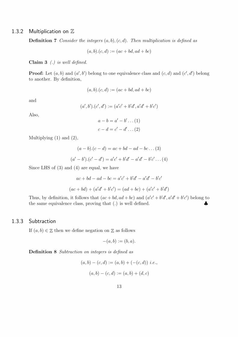
1.3.2 Multiplication on ZDefinition 7 Consider the integers (a, b), (c, d). Then multiplication is defined as

(a, b).(c, d) := (ac+ bd, ad+ bc)

Claim 3 (.) is well defined.

Proof: Let (a, b) and (a′, b′) belong to one equivalence class and (c, d) and (c′, d′) belongto another. By definition,

(a, b).(c, d) := (ac+ bd, ad+ bc)

and(a′, b′).(c′, d′) := (a′c′ + b′d′, a′d′ + b′c′)

Also,a− b = a′ − b′ . . . (1)

c− d = c′ − d′ . . . (2)

Multiplying (1) and (2),

(a− b).(c− d) = ac+ bd− ad− bc . . . (3)

(a′ − b′).(c′ − d′) = a′c′ + b′d′ − a′d′ − b′c′ . . . (4)

Since LHS of (3) and (4) are equal, we have

ac+ bd− ad− bc = a′c′ + b′d′ − a′d′ − b′c′

(ac+ bd) + (a′d′ + b′c′) = (ad+ bc) + (a′c′ + b′d′)

Thus, by definition, it follows that (ac+ bd, ad+ bc) and (a′c′ + b′d′, a′d′ + b′c′) belong tothe same equivalence class, proving that (.) is well defined. ♣

1.3.3 Subtraction

If (a, b) ∈ Z then we define negation on Z as follows

−(a, b) := (b, a).

Definition 8 Subtraction on integers is defined as

(a, b)− (c, d) := (a, b) + (−(c, d)) i.e.,

(a, b)− (c, d) := (a, b) + (d, c)

13

It can be checked that (-) is also well defined, by using the ’well-defined’ness of (+) andthe fact that (−) can be represented in terms of (+).

Claim 4 N ⊆ Z.

Proof: Define a set N := (a, 0) ∈ Z. Now, consider the following map.

f : N 7−→ N

i.e., f : a 7−→ (a, 0)

We observe that f(a + b) = (a + b, 0) and f(a) = (a, 0) , f(b) = (b, 0)⇒ f(a + b) =f(a) + f(b) ∀a, b ∈ N . This map identifies Natural Numbers sitting inside the Integers.♣

Proposition 4 Addition and Multiplication on Z satisfy the following:

1. They are Commutative, Associative and Addition distributes over Multiplication

2. O:=(0,0) satisfies (a,b)+O=(a,b) ∀(a, b) ∈ Z

3. Given m ∈ Z there exists a unique n ∈ Z such that m+ n = 0

4. If m+ x = n+ x , then m = n, ∀ x,m, n ∈ Z

Proof: 3. Let us consider m = (a, b) ∈ Z. Let n = (c, d) ∈ Z such that m+ n = 0.

(a, b) + (c, d) = (0, 0)

(a+ c, b+ d) = (0, 0)

(a+ c)− (b+ d) = 0− 0

(a+ c)− (b+ d) = 0

a+ c = b+ d

a− b = d− c−(a− b) = c− d

(b, a) = (c, d)

Hence (c, d) = (b, a) and this shows existence of additive inverse in Z.

Now, we prove the uniqueness of additive inverse. Let n1 = (c, d) ∈ Z and n2 = (e, f) ∈ Z

14

both be additive inverses for m.

(a, b) + (c, d) = (0, 0) . . . (1)

(a, b) + (e, f) = (0, 0) . . . (2)

(a+ c, b+ d) = (0, 0) . . . (using (1))

(a+ e, b+ f) = (0, 0) . . . (using (2))

(a+ c, b+ d) = (a+ e, b+ f) . . . (from above two)

(a+ c) + (b+ f) = (b+ d) + (a+ e) . . . (from definition)

a+ b+ c+ f = a+ b+ d+ e . . . (using associativity)

c+ f = e+ d . . . (cancellation law)

c− d = e− f(c, d) = (e, f)

Hence (c, d) and (e, f) represent the same integer and hence, we have proved uniquenessof the inverse. ♣

Proof: 4. Let us consider m = (a, b) and n = (c, d) ∈ Z. Let x = (x1, x2) ∈ Z such thatm + x = n + x. For x = (0, 0), we have (a, b) + (0, 0) = (c, d) + (0, 0) ⇒ (a, b) = (c, d).Now, we induct on x1.Assume that m + x = n + x⇒ m = n is true for x = (x1, x2). We now prove this to betrue for x = (x1 + 1, x2).

(a+ x1, b+ x2) = (c+ x1, d+ x2)⇒ (a, b) = (c, d) . . . (given)

(a+ x1)− (b+ x2) = (c+ x1)− (d+ x2)⇒ (a, b) = (c, d)

(a− b) + (x1 − x2) = (c− d) + (x1 − x2)⇒ (a, b) = (c, d)

(a− b) + (x1 − x2) + 1 = (c− d) + (x1 − x2) + 1⇒ (a, b) = (c, d)

(a− b) + ((x1 + 1)− x2) = (c− d) + ((x1 + 1)− x2)⇒ (a, b) = (c, d)

Hence, we have shown that the statement holds for x = (x1 + 1, x2), thus completing theinduction. ♣

1.3.4 Order on ZLet m,n ∈ Z We say m > n if

1. m = n+ p, for some p ∈ Z

2. m 6= n.

15

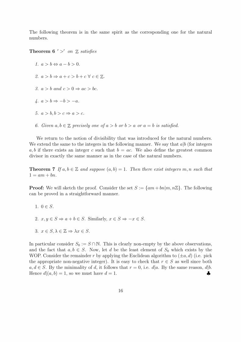
The following theorem is in the same spirit as the corresponding one for the naturalnumbers.

Theorem 6 ′ >′ on Z satisfies

1. a > b⇔ a− b > 0.

2. a > b⇒ a+ c > b+ c ∀ c ∈ Z.

3. a > b and c > 0⇒ ac > bc.

4. a > b⇒ −b > −a.

5. a > b, b > c⇒ a > c.

6. Given a, b ∈ Z precisely one of a > b or b > a or a = b is satisfied.

We return to the notion of divisibility that was introduced for the natural numbers.We extend the same to the integers in the following manner. We say that a|b (for integersa, b if there exists an integer c such that b = ac. We also define the greatest commondivisor in exactly the same manner as in the case of the natural numbers.

Theorem 7 If a, b ∈ Z and suppose (a, b) = 1. Then there exist integers m,n such that1 = am+ bn.

Proof: We will sketch the proof. Consider the set S := am+ bn|m,nZ. The followingcan be proved in a straightforward manner.

1. 0 ∈ S.

2. x, y ∈ S ⇒ a+ b ∈ S. Similarly, x ∈ S ⇒ −x ∈ S.

3. x ∈ S, λ ∈ Z⇒ λx ∈ S.

In particular consider S0 := S ∩N. This is clearly non-empty by the above observations,and the fact that a, b ∈ S. Now, let d be the least element of S0 which exists by theWOP. Consider the remainder r by applying the Euclidean algorithm to (±a, d) (i.e. pickthe appropriate non-negative integer). It is easy to check that r ∈ S as well since botha, d ∈ S. By the minimality of d, it follows that r = 0, i.e. d|a. By the same reason, d|b.Hence d|(a, b) = 1, so we must have d = 1. ♣

16

1.4 Rational Numbers

Again, informally, by the rational numbers, we denote ‘numbers of the formp

q, where

p, q ∈ Z and q 6= 0’. But as we have seen before with the Integers, the path to formalizingthis involves setting up the right kind of equivalence relation on pairs of integers.

Definition 9 We define a Relation ∼ on Z× (Zr0) as

a//b ∼ c//d

if ad = bc, where a, b, c, d ∈ Z and b, d 6= 0.

Remark 3 The integers satisfy the property that there are no zero divisors,i.e. if a, b ∈ Z and ab = 0,then either a = 0 or b = 0 or both a, b = 0. Indeed, if a, b > 0then we have seen from the properties of the natural numbers that ab > 0. If say a < 0,then (−a)b > 0 and this also implies that ab < 0, so in particular, it is not zero. Thesame argument works in the other cases as well.

Proposition 5 ∼ defined on Z× (Zr0) is an Equivalence Relation.

Proof: We prove the three properties of equivalence relations.

1. ReflexivityWe have

a//b ∼ a//b

⇒ ab = ba and this is true.

2. SymmetryWe have , if

a//b ∼ c//d

⇒ ad = bc, then

c//d ∼ a//b

⇒ bc = ad, which is true, since ad = bc.

3. TransitivityIf

a//b ∼ c//d

⇒ ad = bc, and

c//d ∼ e//f

17

⇒ fc = ed, we get

(ad)(fc) = (bc)(ed)

(af)(cd) = (eb)(cd)........(Using Associativity)

(af − eb)(cd) = 0

Let x = cd .We now use the property of no zero divisors for integers. If x 6= 0 weare through, since it implies that af = eb and hence ⇒ a//b ∼ e//f .If x = 0, then cd = 0,⇒ c = 0 , since d 6= 0 by definition. But then, if c = 0, thena = 0 and e = 0 (by definition of the relation) and thus ⇒ a//b ∼ e//f .Since, the relation ∼ is Reflexive , Symmetric and Transitive, it is an EquivalenceRelation.

♣

Remark 4 The set of Rational Numbers, denoted by Q, is the set of equivalence classesof Z×(Zr0) with respect to the equivalence relation ∼ .

1.4.1 Addition and Multiplication on QWe define Addition on Q in the following manner:

(a//b) + (c//d) := (ad+ bc)//bd

We define Multiplication on Q in the following manner:

(a//b).(c//d) := (ac)//bd

We can check that both Addition(+) and Multiplication(.) on Q are well defined as wehave done with the integers.

Claim 5 (.) is well defined for Q.

Proof: Let (a//b) and (a′//b′) belong to one equivalence class and let (c//d) and (c′//d′)belong to another equivalence class.Then by definition,

(a//b).(c//d) := (ac)//bd

(a′//b′).(c′//d′) := (a′c′)//b′d′

18

Also, since (a//b) and (a′//b′) belong to the same equivalence class,we have ab′ = ba′.Similarly, cd′ = dc′ .⇒ (ab′)(cd′) = (ba′)(dc′). By associativity,we have (ac)(b′d′) =(bd)(a′c′). Thus, by definition,

(ac//bd) ∼ (a′c′//b′d′)

and hence (.) is well defined for Q ♣

Claim 6 (+) is well defined for Q

Proof: Let (a//b) and (a′//b′) belong to one equivalence class and let (c//d) and (c′//d′)belong to another equivalence class.Then by definition,

(a//b) + (c//d) = (ad+ bc)//bd

(a′//b′).(c′//d′) = (a′d′ + b′c′)//b′d′

Also, since (a//b) and (a′//b′) belong to the same equivalence class,we have

ab′ = ba′ . . . (1)

Similarly,cd′ = dc′ . . . (2)

Now, multiplying (1) on both sides by dd′ and (2) by bb′, we get

ab′dd′ = ba′dd′ . . . (3)

cd′bb′ = dc′bb′ . . . (4)

By associativity,(3) and (4) can be written as

adb′d′ = a′d′bd . . . (5)

b′d′bc = b′c′bd . . . (6)

Adding (5) and (6), we get

adb′d′ + b′d′bc = a′d′bd+ b′c′bd

Thus,by definition⇒ (ad+ bc)//bd ∼ (a′d′ + b′c′)//b′d′

and hence (+) is well defined for Q. ♣

Theorem 8 (Q is a FIELD)The set of Rationals , along with the binary operations (.) and (+) defined on it satisfythe following:

19

1. Addition and Multiplication on Q are commutative , associative and (+) dis-tributes over (.) .

2. Z is a subset of Q .i.e., Z 7−→ Q and this can be obtained byn 7−→ (n//1). Therefore, the map identifies Z inside Q and all the operations arecompatible.

3. For x ∈ Q , we have

x+ 0 = x . . . Additive Identityx.1 = x . . . Multiplicative Identity.

4. For x = a//b , there is a unique rational y = −a//b such that x+y = 0. Therefore,Q has a unique Additive Inverse.

5. If x = a//b where a 6= 0 , then there exists unique x−1 := b//a satisfying

x.x−1 = 1 . . . Multiplicative Inverse.

♣

Note 2 For x = (a//b) we define −x := (−1//1).(a//b).i.e., −x = −1.x.

1.4.2 Order on QFor x ∈ Q , we say that

1. x > 0 if , for x = a//b , a, b ∈ N−0

2. x < 0 if −1.x > 0.

3. x = 0 if a = 0 and b 6= 0.

In general , for x, y ∈ Q we say that x > y , if ∃ r ∈ Q and r > 0 such that x = y + r .

Theorem 9 (Total Order) The Rational numbers Q and >,< defined earlier on Qsatisfy the following:

1. For x, y ∈ Q, exactly one of x > y , x < y , x = y is satisfied.(Trichotomy)

2. For x, y, z ∈ Q, x < y ⇒ x+ z < y + z.

3. For x, y, z ∈ Q and z > 0, x < y ⇒ xz < yz.

4. For x < y, −x > −y.

5. For x, y, z ∈ Q , if x < y and y < z , then x < z.

Thus, (Q, (+), (.), <,>) is a Totally Ordered Field. ♣

20

1.4.3 Q misses some ‘numbers’

Before we move to the next important theorem we need a lemma. Recall the definitionof primes (in the set N).

Lemma 3 For a prime number p , if p|ab for natural numbers a, b, then p|a or p|b orboth.

Proof: First, using the Euclidean algorithm we may assume WLOG that a, b ≤ p. Sincep is prime, if p does not divide a, then we must have (a, p) = 1. By a previous theorem,there exist integers λ, µ such that aλ + pµ = 1. Multiplying by b on both sides wehave b = abλ + bpµ. Now, both the terms on the right hand side are divisible by p byassumption. Hence we must necessarily have p|b. ♣

Theorem 10 Fundamental Theorem of ArithmeticEvery Natural number n > 1 can be expressed as a product of primes in a unique way,except for permuting the factors.

Proof:

1. (Existence of the product of primes)We use induction to prove that all natural numbers n > 1 can be expressed as aproduct of primes. For n = 2, it is true since 2 is itself a prime number. Assumethat for all n > 2 and less than N , there is a way to express the numbers as aproduct of primes. Now, consider n = N . If N is prime, we are through. If N isnot a prime, then N can be written as N = ab , where a, b ∈ N and 0 < a, b < N .According to induction, a and b can be expressed as a product of primes. Thus,N = ab can also be expressed as a product of primes.

2. (Uniqueness) Suppose that the number N can be expressed in two ways as

N = pa11 pa22 . . . pamm = qb11 q

b22 . . . qbnn

Here all the pi′s and qj

′s are distinct primes and all ai′s and bj

′s are the numberof times each prime occurs in the product. We want to show that m = n and eachpaii = q

bjj for some j ; i.e., pi = qj and ai = bj . Now, consider p1.We have

pa11 pa22 . . . pamm = qb11 q

b22 . . . qbnn (1)

p1 divides LHS of (1). Hence p1 divides even RHS of (1).⇒ p1|qbjj for some j.

⇒ p1|qj. But since p1 and qj are primes , we must have p1 = qj . Let us renumberthe index j as 1 and vice-versa. We get,

pa11 pa22 . . . pamm = pb11 q

b22 . . . qbnn

21

Now, if a1 > b1 then divide both sides by pb11 to get

pa1−b11 pa22 . . . pamm = qb22 . . . qbnn

We notice that the LHS is now divisible by p1 while the RHS is not.This is notpossible. Similarly we can show that a1 < b1 is also not possible. Hence , the onlypossibility is that a1 = b1.The equation now becomes

pa22 . . . pamm = pb11 qb22 . . . qbnn

Without loss of generality, we will assumem < n. Proceeding similarly for p2, p3 . . . pmwe can cancel terms on both sides until we are left with

1 = qbm+1

m+1 qbm+2

m+2 . . . qbnn

However since the RHS is supposed to be a product of primes which is equal to 1, itimplies that all the terms on the RHS are 1’s and do not contribute to the productof (1). Hence, we will have each of the prime in LHS paired up with a prime in RHSwith equal powers, thus proving the uniqueness of the product expression exceptfor the order in which they occur.

♣

From the fundamental theorem of arithmetic it follows that every rational x canbe expressed asp

qwhere p, q are integers that have no prime factors in common. This

representation of the rationals will be of use to us.Firstly, the rationals are a pretty ‘large’ set. Indeed, we have the following:

Fact 1 If a, b ∈ Q and a < b , then there exists c ∈ Q such that a < c < b.

Indeed, it is easy do check that if a < b ∈ Q then c = 12(a + b) is also in Q and we have

a < c < b.

Proposition 6 There is no Rational Number x such that x2 = 2.

Proof: Let us assume to the contrary that there exists x ∈ Q such that x2 = 2. Writingx as x = p

qwhere p, q ∈ Z,q 6= 0 and p, q have no common factor other than 1.Then we

have,

(p/q)2 = 2 (1.1)

⇒ p2 = 2q2 (1.2)

⇒ 2|p2 (1.3)

⇒ 2|p (1.4)

⇒ p = 2k for some k ∈ N (1.5)

22

Substituting p in (2),we get

⇒ 4k2 = 2q2 (1.6)

⇒ 2k2 = q2 (1.7)

⇒ 2|q2 (1.8)

⇒ 2|q (1.9)

From (4) and (9) , we get 2|p and 2|q which is a contradiction to the assumption thatp, q have no common factor other than 1.Therefore there is no rational number such that x2 = 2.

♣

1.5 Real Numbers

Definition 10 (Dedekind Cut) A Dedekind Cut is a partition A ·∪B of Q satisfying

1. A 6= ∅ , B 6= ∅.

2. For a ∈ A , b ∈ B , we have a < b.

3. A has no largest element

Definition 11 A Dedekind Cut A oB is defined to be a Real number.i.e.,

R = A oB | A oB is a Dedekind cut of Q

Proposition 7 Q ⊂ R, i.e., x ∈ Q⇒ x ∈ R.

Proof: For every x ∈ Q , we define the partition

L = y ∈ Q |y < x,

R = y ∈ Q |y ≥ x,

By this partition, we can associate every x ∈ Q to a corresponding partition L oR whichis a Real Number in R. ♣

Definition 12 (Order on Real Numbers) If x = (L oR) and y = (L’ oR’) are Realnumbers , then x < y if L ⊂ L’.

Definition 13 A non-empty set S ⊆ R is said to be bounded above if there is anx ∈ R, such that for every s ∈ S , s < x. Such an x is called an Upper Bound of S.

23

Theorem 11 Every non empty set S ⊆ R which is bounded above has a least upperbound (lub).i.e., ∃y ∈ R satsifying

1. s ≤ y, ∀ s ∈ S.

2. If y′ satisfies s ≤ y′ ∀ s ∈ S , then y ≤ y′ .

Proof: Let s = (Ls oRs) . Let L = ∪s∈S Ls and R = QrL.

1. CLAIM: y = (L oR) will do.First, L 6= ∅ and R 6= ∅, since every rational upper bound for S is not in Ls forany s. Further, for a ∈ L and b ∈ R, we have a ≤ b. Lastly, it is not hard to seethat L has no greatest element since such an element must necessarily be in someof the Ls which is not possible by assumption. Now we have Ls ⊂ L and thereforefor every s ∈ S we have s ≤ y .

2. Suppose there exists another number y′ such that y′ ≥ s ∀s ∈ S. Since y′ ≥ s ∀s ,by definition we have Ly′ ⊇ Ls ∀s ∈ S,

⇒ Ly′ ⊇ ∪s∈SLs

⇒ y′ ≥ y.

♣

Example 2 The real number√

2 can be obtained as the following Dedekind cut L o Rdefined as:

L = x ∈ Q |x ≤ 0 or x2 < 2

R = QrL.

We will in fact prove something stronger and more general later.

1.5.1 Addition and Multiplication on RWe define Addition on R in the following manner:

x = (Lx oRx)

andy = (Ly oRy),

x+ y = (Lx+y oRx+y),

24

whereLx+y := Lx + Ly := r + s | r ∈ Lx, s ∈ Ly.

Rx+y := Q \Lx+y.

We define Multiplication on R in the following manner:

First consider the case of positive cuts where x, y ≥ 0.Then

Lx.y := r ≤ 0 ∪ a.b | a ∈ Lx, b ∈ Ly, a, b ≥ 0

For the remaining cases, we need to define the notion of negative cut.

Definition 14 Ify = (Ly oRy) ∈ R

thenL−y := r | r = −s for some s ∈ Ry, s is not min(Ry)

Now,

If x ≥ 0, y ≤ 0x.y := −(x.(−y)).

If x ≤ 0, y ≥ 0x.y := −((−x).y).

If x ≤ 0, y ≤ 0,x.y := (−x).(−y).

One can prove (we omit the rather laborious proof) that

Theorem 12 (R,+, ·) is a field. ♣

The next proposition shows that the set of reals constructed this way does not have ‘gaps’the way the set of rationals did.

Proposition 8 R has no gaps.

Proof: Suppose A oB is a partition of R s.t

1. A, B 6= Ø, A ∪ B = R, A ∩ B = Ø.

2. For a ∈ A , b ∈ B , we have a < b.

25

3. A has no largest element.

By (2) each b ∈ B is an upper bound for A ⇒ A is bounded above ⇒ x = lub(A)exists.Since x = lub(A), we have

a ≤ x, for all a ∈ A ( x is a least upper bound ),

x ≤ b for all b ∈ B (each b is also an upper bound for A),

so it follows that

a ≤ x ≤ b for all a ∈ A , b ∈ B.

Consider

A′ = r ∈ Q ‖ r < x

B′ = r ∈ Q ‖ r ≥ x

x = A′ oB′

Claim 7

A = y ∈ R ‖ y < x

B = y ∈ R ‖ y ≥ x

Indeed,

A ⊆ y ∈ R ‖ y < x

clearly it is true as x = lub(A) and moreover

y ∈ R ‖ y < x ⊆ A.

The last holds since otherwise there is y < x, y /∈ A⇒ y ∈ B. But each b ∈ B satisfiesx ≤ b and this contradicts y < x.The other parts are proven similarly. ♣

The following theorem (whose proof we skip as the details are laborious) consolidatesour understanding of the reals.

Theorem 13 (R, (+), (.), <,>) is a Totally Ordered Field. ♣

26

1.5.2 Another description for Real Numbers

Before we go there, here is a remarkable property of R.

Definition 15 A real number x is called IRRATIONAL if x ∈ RrQ

Notation: Suppose a < b, a, b ∈ R.

(a, b) = x ∈ R ‖ a < x < b.

[a, b] = x ∈ R ‖ a ≤ x ≤ b.

(−∞, a) = x ∈ R ‖ x < a.

(−∞, a] = x ∈ R ‖ x ≤ a.

(b,∞) = x ∈ R ‖ x > b.

[b,∞) = x ∈ R ‖ x ≥ b.

Theorem 14 For every a < b, the interval (a, b) contains both rational and irrationalnumbers.

Proof:√

2 ∈ RrQ⇒ 1√2∈ RrQ.

Also we know that 12∈ Q and in fact, 1

2∈ (0, 1) since if 1

2> 1, then multiplying by 2 on

both sides, we get 1 > 2 which is a contradiction.Thus for a = 0, b = 1 we are through.Now let a = A oB, b = A

′ oB′ and a < b⇒ A ⊂ A

′ ⇒ ∃r, s ∈ A′ r A.WLOG, r < s ⇒ a ≤ r < s ≤ bNow, consider the function, f : (0, 1)→ (r, s) defined as f(x) = r + x(s− r).Clearly, f maps rationals to rationals and this property is also satisfied by its inverse,which exists as f is a bijection.⇒ f(1

2) ∈ Q, f( 1√

2) ∈ RrQ and they lie in (a, b). ♣

Theorem 15 For all x > 0, and n ≥ 2, n ∈ N, there exists a unique y > 0 such thatyn = x or equivalently, we write y = n

√x

Proof: Suppose x > 1 (WLOG, this is the only case we have to deal with).Let R = r > 0‖ rn ≤ x. Clearly, R 6= ∅ as 1 ∈ R.

Claim 8 R is bounded above.

x > r for all r ∈ R. A simple induction argument shows that xn ≥ x. Also, bydefinition, x /∈ R so R is bounded above. Hence y = lub (R) exists.

27

Claim 9 yn = x.

We will use the Trichotomy law for showing that equality holds, i.e., we shall showyn ≥ x and yn ≤ x.As y = lub(R), we have r ≤ y for any r ∈ R. Now, for any r ∈ R we have r ≤ y ⇒ r.r ≤y.r (as r > 0). Hence r2 ≤ y2. Similarly, rn ≤ yn. (by induction) ⇒ yn ≥ x.

For the other case consider A = (y − ε)n‖ 0 < ε < y.

Claim 10 x is an upper bound for A.

y = lub(R)

⇒ y − ε is not an upper bound forR.

Claim 11 (y − ε)n ≤ x.

Since y−ε is not an upper bound for R, there exists r ∈ R such that (y−ε)n ≤ rn ≤ x⇒ x is an upper bound for A.

Claim 12 yn = lub(A)

Suppose not. Clearly, yn is an upper bound.Let yn − δ be the lub for A for some fixed δ > 0So

(y − ε)n ≤ yn − δ for all 0 < ε < y, which implies

δ ≤ yn − (y − ε)n

≤ ε(yn−1 + yn−2(y − ε) + .....(y − ε)n−1)

≤ εnyn−1

for all 0 < ε < y. If ε = δ2nyn−1 < y then we have δ ≤ δ

2for δ > 0 which is a contradiction.

So, yn = lub(A) ≤ x, and this completes the proof that yn = x. ♣

1.5.3 Archimedian Property of RProposition 9 For any real x > 0, there exists a unique n ∈ N s.t n ≤ x < n+ 1.

Proof: Let x ∈ R, x = A oB. For p, q ∈ N, pick

p

q∈ B,

p

q> x > 0, and p, q > 0.

Thenp

q<

p

q+

p

q+

p

q+ ..... +

p

q= p.

28

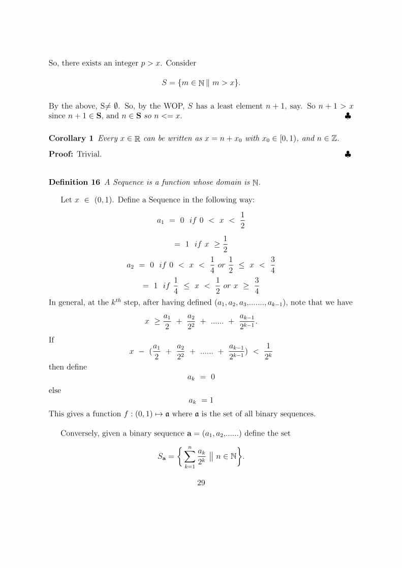
So, there exists an integer p > x. Consider

S = m ∈ N ‖ m > x.

By the above, S6= ∅. So, by the WOP, S has a least element n + 1, say. So n + 1 > xsince n+ 1 ∈ S, and n ∈ S so n <= x. ♣

Corollary 1 Every x ∈ R can be written as x = n+ x0 with x0 ∈ [0, 1), and n ∈ Z.

Proof: Trivial. ♣

Definition 16 A Sequence is a function whose domain is N.

Let x ∈ (0, 1). Define a Sequence in the following way:

a1 = 0 if 0 < x <1

2

= 1 if x ≥ 1

2

a2 = 0 if 0 < x <1

4or

1

2≤ x <

3

4

= 1 if1

4≤ x <

1

2or x ≥ 3

4

In general, at the kth step, after having defined (a1, a2, a3,......., ak−1), note that we have

x ≥ a1

2+

a2

22+ ...... +

ak−1

2k−1.

If

x − (a1

2+

a2

22+ ...... +

ak−1

2k−1) <

1

2k

then defineak = 0

elseak = 1

This gives a function f : (0, 1) 7→ a where a is the set of all binary sequences.

Conversely, given a binary sequence a = (a1, a2,......) define the set

Sa =

n∑k=1

ak2k∥∥ n ∈ N

.

29

Since each element of S is strictly less than 1, lub(S) exists for each binary sequence.

To summarize: For every x , 0 < x < 1 we can associate a binary sequence ax ,and conversely, for each binary sequence a we can define a real number in (0,1) byx = lub(Sa).

Question 1: If 0 < x < y < 1, then can we have ax = ay? In other words, if x < ythen is it true that ak(x) 6= ak(y) for some k?

If y − x = δ > 0, pick n such that δ > 12n

. Suppose ax = ay i.e ax(i) = ay(i) for alli ∈ N. Then

x > Σax(i)

2i= Σ

ay(i)

2i> y − 1

2n,

so that we have

y − x <1

2n⇒ δ <

1

2n,

which is a contradiction. Hence, distinct elements of (0, 1) give distinct binary sequencesby this mapping. In other words, x→ ax is an injection.

Question 2: If a1 6= a2, is lub(S1) 6= lub(S2)?

This is not the case. Considera1 = (1, 0, 0, 0..., ) and a2 = (0, 1, 1, 1...). Both ‘represent’ the same number.

Proposition 10 The sequence a = (1, 1, 1...) has lub(Sa) = 1.

Proof: Clearly 1 is an upper bound. Suppose lub(Sa) = 1− δ ∃ δ > 0. Then Σk≤n12k≤

1− δ for all n ∈ N. But then 1− 12n≤ 1− δ ⇒ δ ≤ 1

2nfor all n ∈ N. By the Archimedean

property, there exists N ∈ N such that N > 1δ. Now, one can prove by induction, that

2N > N for all N ∈ N, so this gives 2N > 1δ. This is a contradiction. ♣

A consequence of the above proposition is the following. For any sequence a whichterminates in ones, i.e. ai = 1 for all i ≥ N0 for some N0 there is another binary sequenceb such that bi = 0 for all i ≥ N0 and lub(Sa) = lub(Sb). Let us now denote by A the setof all binary sequences that do NOT terminate in ones.

We now can prove the following

Theorem 16 The maps F,G,

F : A → (0, 1), defined as F (a) = lub(Sa),

G : (0, 1) → A, defined as G(x) = ax

as defined in class, are inverses of each other, i.e., F (G(x)) = x,G(F (a)) = a.

30

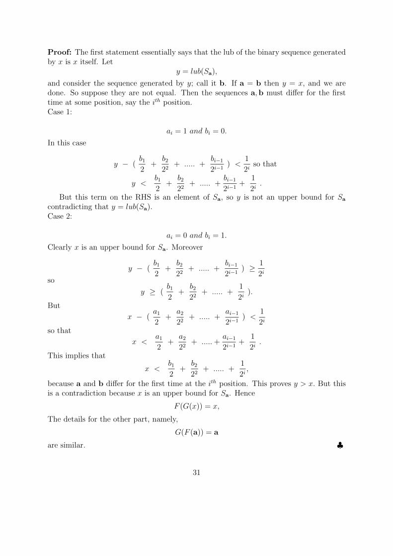
Proof: The first statement essentially says that the lub of the binary sequence generatedby x is x itself. Let

y = lub(Sa),

and consider the sequence generated by y; call it b. If a = b then y = x, and we aredone. So suppose they are not equal. Then the sequences a,b must differ for the firsttime at some position, say the ith position.Case 1:

ai = 1 and bi = 0.

In this case

y − (b1

2+

b2

22+ ..... +

bi−1

2i−1) <

1

2iso that

y <b1

2+

b2

22+ ..... +

bi−1

2i−1+

1

2i.

But this term on the RHS is an element of Sa, so y is not an upper bound for Sa

contradicting that y = lub(Sa).Case 2:

ai = 0 and bi = 1.

Clearly x is an upper bound for Sa. Moreover

y − (b1

2+

b2

22+ ..... +

bi−1

2i−1) ≥ 1

2iso

y ≥ (b1

2+

b2

22+ ..... +

1

2i).

But

x − (a1

2+

a2

22+ ..... +

ai−1

2i−1) <

1

2i

so that

x <a1

2+

a2

22+ .....+

ai−1

2i−1+

1

2i.

This implies that

x <b1

2+

b2

22+ ..... +

1

2i,

because a and b differ for the first time at the ith position. This proves y > x. But thisis a contradiction because x is an upper bound for Sa. Hence

F (G(x)) = x,

The details for the other part, namely,

G(F (a)) = a

are similar. ♣

31

1.6 Cardinality

Until now, we have talked a great deal about natural numbers, integers, rationals andthen the reals, but haven’t had a look at the sizes of these sets. A measure of the numberof elements in any set in general motivates the idea of cardinality.

Definition 17 We say that two sets A and B have the same cardinality iff ∃ a bijectionh : A B

Definition 18 Set A is said to have cardinality n (for some n ∈ N if A has samecardinality as 0,1,2,...,n-1 (or equivalently 1,2,...,n). We write it as : |A| = n

Remark 5 We denote the set 1,2,...,m by [m].

Proposition 11 Given m,n∈ N where m < n, there is no injection f : [n]→ [m].

Proof: Let S = n ∈ N | ∃m ∈ N,m < n such that there is an injection fnm : [n]→ [m]We now need to prove that S = Φ.If not, then by the Well-Ordering Principle, it must have a least element (say n0) and acorresponding m < n0.Let h be the injection h : 1, 2, ..., n0 → 1, 2, ...,m. Consider the value h(n0).

Case I: h(n0) = mConstruct the function h’ such that

h′ : [n0 − 1]→ [m− 1]h′(i) = h(i)∀ i ∈ 1, 2, ..., n0 − 1

Then h’ is also an injection. Hence (n0− 1) ∈ S which contradicts the fact that n0 is theleast element of S.

Case II: h(n0) 6= mSuppose h(n0) = k, k < mLet π be the map (km), i.e., the map that permutes k and m.Then, we have an injection π h : [n] [m] with (π h)(n) = m which is a functionsatisfying Case I, hence again leading to a contradiction.So, our assumption was wrong. S must be Φ. ♣

Corollary 2 If A [n], then we cannot have A [m] for any m 6= n.

Definition 19 We say that a non-empty set A is INFINITE iff there is no n ∈ N suchthat |A| = n.

Remark 6 |Φ| := 0.

32

Proposition 12 N is infinite.

Proof: Suppose f : N [n] for some n. In particular, restrict f to [n+ 1]. This definesan injection f ′ : [n+ 1] [n] which is a contradiction. ♣

Proposition 13 Suppose A ⊆ N. Then either |A| = n for some n ∈ N0 or A has thesame cardinality as N.

Proof: If A ⊆ N is finite, we say that |A| = n for some n ∈ N0. Also, if A = N, we arethrough. So, the only thing that remains to be proved is that if A is infinite and A 6= N,there exists

f : A N

Since A 6= Φ, it has a least element, say a1. Let A0 = A.Consider A1 = A0 \ a1. A1 must be infinite. Because if it weren’t, then A0 would havejust one more element than A1 and hence also be finite.So, there must exist a minimum element in A1, say a2. Construct A2 = A1 \ a2.Inductively, obtain an+1 = min(An); An+1 = An \ an+1The bijection is:

f : N→ Af(i) = ai

f is clearly injective since ai < aj∀i < j. Hence also observe that ai ≥ i (can be provedusing induction). We now need to prove surjectivity of f .Suppose f is not surjective. Since A 6= N, we must have an x ∈ A such that ax > x andx 6= ai∀i. But in this case, x ∈ Ax−1 and x < ax which is a contradiction. So, f must besurjective and hence bijective too. ♣

Corollary 3 There are as many primes as elements of N.

Remark 7 We write |A| <∞ if |A| = n for some n ∈ N0.If |A| <∞, B ⊂ A, then |B| < |A|.

Definition 20 We say that a set is countable (countably infinite) if it has same cardi-nality as N.

Observations:

1. |Even naturals| = |N |This is because we have the bijection

f : 2N Nf(2k) = k

33

2. |Z | = |N |We can build the bijection here as

f : N Zf(2k) = k

f(2k + 1) = −k

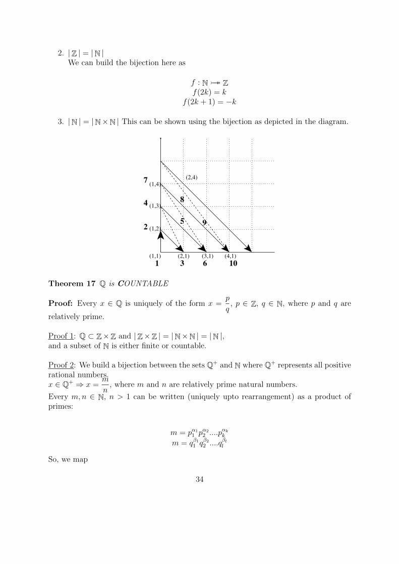
3. |N | = |N×N | This can be shown using the bijection as depicted in the diagram.

(1,2)

(1,3)

(2,4)

(4,1)

(1,4)

(1,1) (3,1)(2,1)

2

3

4

6 101

7

95

8

Theorem 17 Q is COUNTABLE

Proof: Every x ∈ Q is uniquely of the form x =p

q, p ∈ Z, q ∈ N, where p and q are

relatively prime.

Proof 1: Q ⊂ Z×Z and |Z×Z | = |N×N | = |N |,and a subset of N is either finite or countable.

Proof 2: We build a bijection between the sets Q+ and N where Q+ represents all positiverational numbers.x ∈ Q+ ⇒ x =

m

n, where m and n are relatively prime natural numbers.

Every m,n ∈ N, n > 1 can be written (uniquely upto rearrangement) as a product ofprimes:

m = pα11 p

α22 ....p

αkk

m = qβ11 qβ22 ....q

βll

So, we map

34

m

n7→ (p2α1

1 p2α22 ....p2αk

k q2β1−11 q2β2−1

2 ....q2βl−1l )

This is a bijection as an even exponent will map to a factor in the numerator while anodd one will give me one in the denominator. ♣

What about R? Is it also countable?

In the following material, we attempt to answer this particular question.

Definition 21 For a set A, the power set of A is defined as P(A) := B|B ⊆ A.

Theorem 18 |N | 6= |P(N)|

Proof: Here, we simply show that there can’t be an injection from P(N) to N.Identify P(N) with binary sequences in the following way:Given A ⊆ N, for i ∈ N, aA(i) = 1 if i ∈ A and 0 otherwise.Suppose if possible that such an injection exists.

f : N 7→ BinarySequences

Construct the binary string b such that bi = 1 if f(i) has 0 at ith position and o otherwise.Then, b can’t be the image of any natural number and hence f cannot be surjective,leading to the fact that the injection we wanted can’t exist. ♣

Observation: If x ∈ R is associated with binary string α where α ends in all zeroes,then x ∈ Q.

Theorem 19 R is not countable.

Proof: We will show that there is no bijection from from the real numbers in (0,1) to

N. We once again use the idea of identifying elements (real numbers in this case) withstrings. The only difference being that we use ternary strings instead of binary in orderto avoid dealing with such strings that end in all 1s.

Each real number between 0 and 1 can be represented in ternary notation as a string of0s, 1s and 2s, leading to a one-to-one mapping between (0,1) and the set T of all ternarystrings on 0,1,2.Suppose f is a bijection from N to T .

Using Cantor’s diagonalization idea,Construct a ternary string t wherein ti = 0 if f(i) has 1 or 2 in the ith position and 1otherwise. Then t cannot be the image of any natural number, ruling out the possibilityof the existence of a bijection between (0,1) and N. ♣

35

Proposition 14 |(0, 1)| = |R |

Proof: Construct the bijection:

f : (0, 1)→ Rx 7→ 2x− 1

2x(1− x)

♣

Definition 22 We say that |A| ≥ |B| if there is an injection f : B A.

Theorem 20 (SCHRODER-BERNSTEIN)If |A| ≤ |B| and |B| ≤ |A|, then |A| = |B|.

Proof: Consider two sets A and B such that there is an injection f from A to B and aninjection g from B to A. Construct the sequences:

A0 = A, A1 = g f(A0, A2 = g f(A1, ....B0 = B, B1 = f g(B0, B2 = f g(B1, ....

We can define our bijections between Ai−1 \ Ai and Bi−1 \Bi, i ≥ 1.In the figure that follows, the blue parts are in bijection and so are the ones in white.

g(B) f(A)

fg(B)gf(A)

f

gA B

Consider the blue parts. Under f , the range of A is f(A) which is precisely the blue andyellow coloured parts in B. Also, the range of g(B) is the yellow coloured part in B. So,since f is an injection, the range of A \ g(B) must be the blue part in B, meaning thatthe two blue parts are in bijection.By symmetry, the two white parts are also in bijection. Hence, extending this argumentto the entire sequence, we will need to show that Ares and Bres are in bijection where

36

Ares = A \ (⋃i≥1Ai−1 \ Ai)

Bres = B \ (⋃i≥1Bi−1 \Bi)

Claim: f(Ares) = Bres. Suppose there exists a y ∈ Bres which does not have a pre-imagein Ares under f . Say f(x) = y. Then x ∈ (

⋃i≥1Ai−1 \ Ai). But this means that x ∈ Ai

for some i. Then y ∈ Bres is a contradiction.Therefore, Ares and Bres must be in bijection and this completes our proof. ♣

Remark 8 So, we say that A and B are in bijection if we have two injections, one fromA to B and one from B to A.

Examples: Consider the two sets (0,1) and [0,1]. The two injections are as follows:

f : (0, 1)→ [0, 1]x 7→ x g : [0, 1]→ (0, 1)

x 7→ 2x+ 1

4

Theorem 21 For any set A, |A| < |P(A)|

Proof: If A is finite, we have |P(A)| = 2|A|. Now, we need to prove the theorem forinfinite sets. Suppose there is a bijection between A and P(A)| where A is infinite.

f : A→ P(A) = B ⊆ A a 7→ f(a)

Construct B := a ∈ A| /∈ f(a).Suppose f−1(B) = b⇒ B = f(b).If b ∈ B, then b /∈ B.If b /∈ B, then b ∈ B.This is a contradiction. Hence such a bijection cannot exist. ♣

37

1.7 The Complex Numbers

A simple algebraic equation like X2 = −1 may not have a real solution. Introducing com-plex numbers validates the so called fundamental theorem of algebra: every polynomialwith a positive degree has a root (though we will not prove that here).

Definition 23 A complex number is a pair z = (a, b) where a, b ∈ R and we writez = a+ ib.

R×R ≈ C as sets.

Consider two complex numbers z1 = (a1, b1) and z2 = (a2, b2)

1. z1 + z2 = (a1 + a2, b1 + b2)

2. z1z2 = (a1a2 − b1b2, a1b2 + a2b1)

3. z1 = (a1,−b1). This is called the conjugate of z1.

4. |z1| =√a2

1 + b21. Note that |z1| = 0 iff a1 = b1 = 0.

5. For z1 6= 0, z−11 =

z1

|z|2and z z−1 = 1.

Proposition 15 C along with the operations +, · as defined above make it a field withadditive and multiplicative identities being 0, 1 respectively. However, there is no totalorder on C, satisfying the following order properties:

• a ∈ C⇒ a > 0, a = 0 or a < 0.

• a, b > 0⇒ a+ b > 0.

• a > 0, b > c⇒ ab > ac.

Proof: We will only prove the latter statement here. Suppose if possible that there existsa total order on C satisfying the properties listed above.

Since i 6= 0, i must be either less than or greater than 0.Suppose i > 0, then i.i = i2 = −1 > 0 where −1 ∈ C. Hence −1 × −1 = 1 > 0 where1 ∈ C. −1 > 0 and 1 > 0 ⇒ −1 + 1 = 0 > 0 which is a contradiction. Hence, i must beless than 0 for which we can find a similar contradiction. ♣

38

2 Basic Topology

2.1 Metric Spaces

We start with some basic inequalities.

1. x ∈ R =⇒ x2 ≥ 0;x2 = 0; iff x = 0.

2. x ∈ R =⇒

|x| :=

x if x ≥ 0

−x if x < 0

Clearly, x ≤ |x| for all x ∈ R.

Theorem 22 The Triangle Inequality:

x+ y ∈ R =⇒ |x+ y| ≤ |x|+ |y|.

Proof: x + y ≤ |x| + |y|, comes from adding x ≤ |x|, y ≤ |y| for all x ∈ R and y ∈ R.The other inequality, namely, −(x+ y) ≤ |x|+ |y|, comes from adding −x ≤ |x|,−y ≤ |y|for all x ∈ R and y ∈ R. ♣

Definition 24 Metric Space: A metric space is a set X, along with a function d :X× X→ R+ (R+ = x ∈ R|x ≥ 0) satisfying:

1. d(x, y) = d(y, x),for all x, y ∈ X.

2. d(x, y) = 0 if and only if x = y for all x, y ∈ X.

3. Triangle Inequality: d(x, y) ≤ d(x, z) + d(y, z) for all x, y, z ∈ X.

Here are some examples:

1. X = R, d(x, y) = |x− y|.

2. X = Q, d(x, y) = |x− y|.

39

3. X = C, d(z, w) = |z − w|.

4. X = 0, 1n, x, y ∈ X i.e x, y are binary strings. d(x, y) = #1 ≤ i ≤ n|xi 6= yi.

5. One of the most commonly used metrics is X = R2 = R × R, with the distancefunction defined as d((x, y), (x′, y′)) =

√(x− x′)2 + (y − y′)2.

6. One also uses the other metric (called the Taxicab metric) on R2 with the distancefunction d((x, y), (x′, y′)) = |x− x′|+ |y − y′|.

Definition 25 Limit point: Suppose A ⊆ R. We say that x ∈ R is a Limit point of Aif for any ε > 0 we have (x− ε, x+ ε) ∩ (A− x) 6= ∅.

Definition 26 Cauchy sequence: A sequence xn in the reals is called a Cauchy se-quence if given ε > 0 there exists Nε ∈ N such that for all m,n ∈ Nε we have |xn−xm| < ε.

The following proposition is an immediate consequence.

Proposition 16 If xn is Cauchy the the set xn is bounded. Equivalently, thereexists M > 0 such that xn ∈ [−M,M ] for all n ∈ N.

Proof: For ε = 12, there exists N = N 1

2such that for all n ≥ N, xn ∈ (xN − 1

2, xN + 1

2).

Let

M = |x1|+ |x2|+ . . . |xN |+1

2.

We claim that this value of M does the job as stated in the proposition.

Now for all n < N, xn < |xn|+ 12, so xn < M . Also if n ≥ N , then

xn − xN ∈ (−1

2,1

2) =⇒ |xn − xN | <

1

2,

=⇒ |xn| − |xN | <1

2,

=⇒ xn < |xn| < |xN |+1

2,

=⇒ xn < M.

♣

Example 3 xn = (−1)n 1n

. Is xn Cauchy?

40

Suppose n < m. Then

|xn − xm| = |(−1)n 1

n− (−1)m+n

m|,

= | 1n− (−1)m+n

m|,

≤ 1

n+

1

m<

2

n.

Consider an ε > 0. By the archimedian property, n0 ≤ 2ε< n0 + 1 for some n0. So

2n0≥ ε ≥ 2

n0+1. Therefore |xn − xm| < ε, for every n > n0. Hence this sequence is indeed

Cauchy.

Proposition 17 Suppose xnis Cauchy. Then the set xn contains at most one limitpoint.

Proof: Suppose x < y and x, y are both limit points of xn|n ∈ N. Since x is a limitpoint of xn|n ∈ N= A. For every small enough ε > 0, the set (x − ε, x + ε) ∩ A isinfinite. Similarly, (y − ε, y + ε) ∩ A is infinite. Since xn is Cauchy, there exists Nε

such that for all m,n ≥ Nε, |xn − xm| < ε. By (the first observation above there existsn ≥ Nε, such that xn ∈ (x − ε, x + ε) ∩ A. In the same vein, there exists m ≥ Nε, suchthat xm ∈ (y − ε, y + ε) ∩ A. This gives |xn − xm| < ε. However, on the other hand, forany α ∈ (x− ε, x+ ε),β ∈ (y − ε, y + ε)

|α− β| ≥ (y − ε)− (x+ ε),

= y − x− 2ε,

≥ 98y − x100

,

= 98ε,

where ε = y−x100

; this gives a contradiction and our proof is complete. ♣

Definition 27 For any metric (X, d), for any point x ∈ X,we define the open ball ofradius r at x asBr(x) := y ∈ X|d(x, y) < r.

Remark 9 One defines a limit point in an arbitrary metric space in the same manneras in the case of the real line. Indeed, for A ⊆ X, we say that a is a limit point of the setA if and only if Ba(ε) ∩ Ar a 6= ∅ for every r > 0.

We also define a Cauchy sequence in a metric space in the same manner.

Definition 28 Cauchy Sequence in X: xnis Cauchy in X iff for every ε > 0, thereexists Nε ∈ N such that for m,n≥ Nε, we have d (xm, xn) < ε.

41

The following proposition follows along the same lines as the real case.

Proposition 18 A Cauchy sequence in (X, d) has atmost one limit point.

However, in the case of the reals, we are guaranteed a limit point as the following theoremstates

Theorem 23 Every Cauchy sequence in R has a limit point.

Remark 10 Not all metric spaces enjoy this privilege. Indeed, the metric X = Q hasCauchy sequences that do not have any limit in Q.

Proof: Suppose xn is Cauchy. As seen before, xn is bounded, i.e., there exists M > 0such that xn ∈ [−M,M ] for all n ∈ N. Consider

A = a ∈ R | a ≤ xn for infinitely many n .

Clearly, A 6= ∅ since −M ∈ A. Also, A ⊆ [−∞,M ]. So, A is non-empty and boundedabove. Let (A) = x.

Claim 13 x is a limit point for the sequence xn. In other words, for any ε > 0, (x− ε, x+ ε)contains some xn.

Suppose not. Then there exists some ε > 0 such that (x− ε, x+ ε) has no element ofxn. Since x = lub (A) x − ε is not an upper bound for A, so there exist infinitely manyxn > x− ε. But this implies that all elements of xn greater than x− ε must in fact belarger than x+ ε. This gives x+ ε ∈ A, a contradiction since x = lub (A). This completesthe proof of the claim, and consequently, every Cauchy sequence in R has a limit point.♣

We say that a set A ∈ X is bounded if A ⊂ Br (x) for some x ∈ X and a suitabler > 0. The following proposition is also easy.

Proposition 19 In a metric space, every Cauchy sequence is bounded.

Definition 29 Given xn ⊆ X, we say that xn converges to a limit if it is Cauchyand has a limit point.

In symbols, limn→∞

xn = x if for any ε > 0 there exists Nε ∈ N such that for all n ≥ Nε

we have d (xn, x) < ε.

Example 4 xn = 1n

Claim 14 limn→∞1n

= 0| 1n− 0| = 1

n< ε for large enough n ( Archimedian Property )

42

Proposition 20 (X = R, |.|) Suppose xnand ynare sequences in R. Let

limn→∞

xn = X, limn→∞

yn = Y.

1. limn→∞ xn ± yn = X ± Y .

2. limn→∞ λ.xn = λ.X.

3. limn→∞ xn.yn = X.Y .

4. If yn 6= 0 for all n > N for some N and limn→∞ yn 6= 0. then limn→∞xnyn

= XY

.

Proof: We only write the proofs for statements (3), (4) in the proposition above.

limn→∞

xn.yn = X.Y

|xn.yn −X.Y | = |xn.yn −X.yn +X.yn −X.Y |≤ |yn|.|xn −X|+ |X|.|yn − Y |

If x = 0, then the second term vanishes; otherwise choose N1ε such that |yn−Y | < ε2|x|

for all n ≥ N1ε . Since limn→∞ yn = Y , |yn| ≤M for some M > 0 for all n ∈ N.

So, for the first term pick N2ε such that |xn −X| < ε2M

. Hence,

|xn.yn −X.Y | < M.ε

2M+ε

2= ε.

We need to show that 1yn

converges to 1y. Now,

| 1

yn− 1

Y| = |Y − yn|

|Y ||yn|.

Suppose limn→∞ yn = Y 6= 0. Then there exists Nε such that for all n ≥ Nε (where

ε = |Y |2

) ,we have |yn − Y | < |Y |2

. This implies yn ≥ |Y |2

=⇒ |Y−yn||Y ||yn| ≤ 2. |Y−yn||Y |2 for all

n > N . Pick N∗ ≥ N such that |Y − yn| < |y|2ε2

for n ≥ N∗. ♣

The following proposition is often useful in deducing the existence of a limit of asequence.

Proposition 21 Suppose xn is increasing and bounded above, then limn→∞ xn existsand equals lub(xn).

The same conclusion also holds if the sequence is decreasing and bounded below.

43

Example 5 If x > 0 and 0 < x < 1 let xn = xn. Note that xn > xn+1 (This can beproved by Induction.), so xn is decreasing. By the previous proposition, since x > 0 forall n, limn→∞ x

n = L exists and limn→∞ xn+1 = L as well. Hence,

L = limn→∞

xn+1 = x. limn→∞

xn = x.L,

so

=⇒ L. (1− x) = 0 =⇒ L = 0.

If x > 1 then xn is not bounded. Indeed, suppose not, i.e., suppose xn ≤ M for all n.Then xn < xn+1 so xn is increasing. But then by the proposition above the limit wouldexist, and then by the same argument the limit would be zero. But since x > 1 thesisleads to a contradiction.

Proposition 22 e := limn→∞(1 + 1

n

)nexists

Proof: Let xn =(1 + 1

n

)n. We show that xn is increasing and bounded above. Indeed,

xn =

(1 +

1

n

)n,

= 1n + n1

n+n (n− 1)

2!

(1

n

)2

+ . . .+n (n− 1) . . . 1

n!

(1

n

)n,

= 1 +n

n+

nn(n−1

n)

2!+ . . .+

nn(n−1

n) . . . .1

1

n!,

Hence,

xn+1 = 1 +n+ 1

n+ 1+

(n+1n+1

) (nn+1

)2!

+ . . .+

(n+1n+1

) (nn+1

). . . .1

1

(n+ 1)!.

We know that 1 − kn+1

> 1 − kn; also, xn+1 has more number of terms of than xn, so it

follows that xn+1 > xn. Also,

xn ≤ 1 +1

1!+

1

2!+ . . .+

1

n!≤ 1 +

1

1+

1

22+

1

23+ . . .+

1

2n< 3.

Since the sequence is increasing and bounded above, by the above proposition the limitexists. ♣

Example 6 limn→∞n√n = 1.

Write n√n = 1 + xn. Then, we have

n = (1 + xn)n

≥ x2n

(n

2

)>

√2

n− 1for n ≥ 2.

44

Now, limn→∞

√2

n−1exists and is equal to 0. Also, xn > 0. So, by the sandwich

theorem, limn→∞ xn = 0 and so limn→∞n√n = 1 + 0 = 1.

2.2 Subsequences

Definition 30 Given a sequence xn in R any sequence xnkk≥1 where nk is anincreasing infinite subset of N is called a subsequence of xn.

Proposition 23 Any subsequence of a convergent sequence converges to same value i.e.,if xn → X then for any subsequence xnk → X as k →∞.

Proof: Given ε > 0, there exists Nε ∈ N such that | xn − x |< ε for all n ≥ Nε. Sincenk is an increasing infinite subset of N, there are atmost finitely many k such thatnk < Nε i.e., for k > kε(for some kε) , we must have nk ≥ Nε. Therefore for all k > kε,we must have | xnk − x |< ε. ♣

Remark 11 The converse of this proposition is not true. For instance the sequence0,1,0,1,0,1..... does not converge even though it has convergent subsequences.

We now state one of the most important theorems in the context of bounded sequences.

Theorem 24 Bolzano-Weierstrass Theorem Every bounded real sequence admits aconvergent sub-sequence.

Proof: Without loss of generality we may assume 0 ≤ xn ≤ 1 for all n. There are twocases to deal with.

Case 1: xn has only finitely many distinct values.

In this case one element x must repeat infinitely many times. Consider that sub-sequence x, x, x, x . . . which clearly converges to x.

Case 2: xn has infinitely many distinct values:

Let A = xn|n ∈ N. Since A is infinite either A∩[0, 12] is infinite or A∩[1

2, 1] is infinite.

Let I1 be one of the intervals [0, 12], [1

2, 1] which contains infinitely many elements of

A.Inductively if Ik = [a, b] then let Ik+1 be one of [a, a+b2

], [a+b2, b] which contains infinitely

many elements of A.

This gives a sequence of intervals I0 ⊃ I1 ⊃ I2 ⊃ I3 · · · such that each Ik containsinfinitely many elements of A.Write

I0 = [a0, b0], I1 = [a1, b1], I2 = [a2, b2] . . .

45

Since the sequence of intervals is nested, it follows that

a0 ≤ a1 ≤ a2 ≤ · · · < b0 and b0 ≥ b1 ≥ b2 ≥ · · · > a0.

Since an is increasing and bounded, limn→∞ an = a exists.

For each k, pick xnk ∈ Ik.

bn is decreasing and bounded below. So bn → b for some b as n→∞.

an < bn , we must have a ≤ b. Note that bk − ak = 12k

. Thus,

limk→∞

(bk − ak) = limk→∞

1

2k= 0 = lim(bk − ak) = lim

k→∞bk − lim

k→∞ak,

which gives b = a.Since ak ≤ xnk ≤ bk, the sandwich theorem implies that xnk is convergent. ♣

Proposition 24 Suppose an is a sequence in [0, 1] and an → a for some a, thena ∈ [0, 1].

Proof: Suppose not. Without loss of generality suppose a > 1; then a > 1 + 1n

for somenatural number n. Then we have (a− δ, a+ δ)∩ [0, 1] 6= ∅ for δ = a− (1 + 1

n). But since

an ∈ [0, 1] (a − δ, a + δ) cannot have any element of an, and this contradicts that anconverges to a. ♣

Remark 12 Suppose I1 ⊃ I2 ⊃ . . . ⊃ In ⊃ . . . is a sequence of bounded closed intervals.Pick xi ∈ Ii; by the Bolzano-Weierstrass theorem, there exists xnk → x for some x ∈ R.By the preceding proposition x ∈ I1. Similarly xnrr≥k → x and xnrr≥k ⊆ Ik. So,x ∈ Ik by the preceding proposition, and therefore x ∈ Ik for all k. This implies that⋂i≥1 Ii 6= ∅.

Remark 13 The above property is not true on all nested families of sets of reals. Con-sider Ik = (0, 1

k). Here I1 ⊃ I2 ⊃ . . . ⊃ In ⊃ . . .. In this case,

⋂i≥1 Ii = ∅.

Definition 31 1. A set U ∈ R is open if for each x ∈ U , there exists a δ = δx > 0for which (x− δ, x+ δ) ⊂ U .

2. A set U ∈ R is closed if U is open.

Any open interval in R is an open set clearly. It is also easy to see that a closedinterval in R is a closed set.

Some Generalities: The following properties are easily verified.

46

1. A is open if and only if A is closed.

2. ∅ is closed; it is also open.

3. A set can be neither open nor closed: U = (0, 1] not open and U = (−∞, 0]∪(1,∞)is not open.

4. If Ai are open then⋃Ai is open.

5. If Ai are closed then⋂Ai is closed.

6. Finite intersection of open sets is open.

7. Finite intersection of closed sets is closed.

8. a is closed.

Remark 14⋂∞n=1(− 1

2n, 1

2n) = 0. This need not be true for infinite sets.

2.3 Continuity

Definition 32 Suppose U ∈ R is open. f : U =⇒ R is said to be continuous at a pointa ∈ U if given ε > 0, there exists δ > 0 such that | x− y |< δ =⇒| f(x)− f(y) |< ε.

Proposition 25 f : U → R is continuous and xn is a sequence in U converges tox ∈ U . Then f(xn)→ f(x).

Proof: Given ε > 0, we need to prove: There exists Nε such that | f(xn)− f(x) |< ε forall n ≥ Nε.

Since f is continuous there exists δ > 0 such that |f(x)−f(y)| < ε whenever |x−y| < δ.Since U is open, there exists δ1 > 0 such that (x − δ1, x + δ1) ⊂ U . Since xn → x thereexists Nε such that | xn − x |< δ1 if n ≥ Nε. Hence for n ≥ Nε,we have | xn − x |< δ=⇒| f(xn)− f(x) |< ε. ♣

Proposition 26 f is continuous at x if and only if every sequence xn =⇒ x, we alsohave f(xn) =⇒ f(x).

Proof: It suffices to prove the sufficiency part of the proposition. Suppose it does nothold, i.e., suppose f is not continuous at some x i.e. given ε > 0 there exists δ > 0 suchthat | x− y |< δ =⇒| f(x)− f(y) |< ε. This is the same as saying that there exists ε > 0such that for every δ > 0, there is some y such that | x− yδ |< δ, but | f(x)− f(yδ) |≥ ε.

In particular, for δ= 1n, (for every n ∈ N), there exists yn such that | x− yn |< 1

nand

| f(x) − f(yn) |≥ ε. Now, yn → x and still f(yn) does not converge to f(x) - thiscontradicts the hypothesis. ♣

47

Proposition 27 A set A ⊆ R is closed if and only if it contains all its limit points.

Proof: Recall that x ∈ R is a limit point of A if and only if for each δ > 0 (x − δ, x +δ) ∩ (A− x) 6= ∅.

Proof of Necessity:

Suppose A is closed. Let x be a limit point of A. If x /∈ A then x ∈ A which im-plies that there exists δ > 0 such that (x − δ, x + δ) ⊂ A. But then for this δ > 0,(A− x) ∩ (x− δ, x+ δ) = ∅. but this contradicts the hypothesis that A is closed.

Proof of Sufficiency:

Suppose A contains all its limit points. It suffices to prove that A is open.Pick x ∈ A. We claim that there exists δ > 0 such that (x− δ, x+ δ) ∩ A = ∅.

Suppose not,then for each δ = 1n, there exists xn ∈ (x − 1

n, x + 1

n) ∩ A. Let B =

xn|n ≥ 1. By definition, x is a limit point of B, but B is contained in A. In otherwords x is a limit point of B ⊆ A, and therefore x ∈ A, contradicting the hypothesis thatx ∈ A. ♣

2.4 Compactness

Recall: For any closed interval [a, b] any sequence xn ⊂ [a, b] contains a convergentsubsequence, whose limit is also in [a, b]. This comes from the fact that [a, b] is a closedset and the Bolzano Weierstrass theorem.

Definition 33 Sequentially Compactness Let K ⊂ R. We say that K is sequentiallycompact if every sequence in K has a convergent subsequence whose limit is also in K .

Example 7 1. The interval [a, b] is Sequentially Compact.

2. Consider A = [0, 1] ∩ Q. This is not sequentially compact since if we considerxn → 1√

2, xn ⊆ A the limit of any of its subsequence does not lie in A.

3. R or N. Neither of these is sequentially compact. Indeed, consider the sequencexn = n. None of its subsequences converge.

Lemma 4 If a set K ⊆ R is sequentially compact, then it is closed.

Proof: Suppose x is a limit point of K and it does not lie in K. Then for everyδ > 0 (x − δ, x + δ) ∩ K 6= ∅, because x is a limit point. In particular for δ = 1

n,

xn ∈ (x − 1n, x + 1

n) ∩ K. So, xn converges to x. So, any subsequence of that sequence

48

would also converge to x. This in particular implies that the limit x should lie in Kbecause K is sequentially compact. So, all limit points of K lie in K. That means K isclosed. ♣

Lemma 5 If a set K ⊆ R is sequentially compact, then it is bounded.

Proof: Suppose K is not bounded, then there is no M ∈ N such that K ⊆ [−M,M ]. Sothere exists a sequence in K such that for xm ∈ K r [−M,M ].

Consider xmm≥1 ⊂ K. As K is sequentially compact, it has a convergent subse-quence xmk. Let xmk → y as k →∞. Now xmk ∈ (y−1, y+1) for all k ≥ k0. Hence,xmk ∈ (−mk,mk) by the choice of the xi’, so

mk+1 ≥ mk,

(y − 1, y + 1) ∈ [−M,M ], for some M

and this yields xmk /∈ [−M,M ], which is a contradiction. ♣

Another Characterization of Continuity: Let U ⊆ R be open in R, f : U 7→ Rand suppose f is continuous i.e., for x ∈ U , given ε > 0, there exists δ > 0 such that|x − y| < δ implies |f(x) − f(y)| < ε. Equivalently, for y∈ (x − δ, x + δ), we havef(y) ∈ (f(x)− ε, f(x) + ε). For a set V ∈ R,

f−1(V ) := u ∈ U |f(u) ∈ V

so that for V = (f(x)− ε, f(x) + ε) we have

f−1(f(x)− ε, f(x) + ε) ⊃ (x− ε, x+ ε)

In other words if V is open in R, f−1(V ) is open in U . The converse is also valid, i.eif f : U → R such that f−1is open in U for every open set V in R, then f is continuous.

For v ∈ V , there exists ε > 0 such that (v − ε, v + ε) ∈ V if f−1 (v − ε, v + ε) = ∅,then there is nothing to prove. Suppose u ∈ U such that f(u) = v. Since f−1(v− ε, v+ ε)is open in U , and contains u, there exists δ > 0 such that (u− δ, u+ δ) ∈ f−1(v− ε, v+ ε).

For the next lemma, we need a definition.

Definition 34 A collection of open sets U in R is called an open cover for a set K if

K ⊂⋃U∈U

U.

Lemma 6 Lebesgue Number Lemma: Given a set K that is sequentially compact andan open covering U for K, there exists δ > 0 such that for each x ∈ K, (x− δ, x+ δ) ⊂ Ufor some U ∈ U.

49

Proof: Suppose not. For every δ > 0 , there exists x ∈ K such that (x − δ, x + δ) * Ufor any U ∈ U. In particular take δ = 1

n, get xn ∈ K such that (xn − δ, xn + δ) * U for

all U ∈ U i.e (xn − 1n, xn + 1

n) * U ,for all U ∈ U.

Consider xn in K, this has a convergent subsequence xnk → x in K. Now if x ∈ U0

for some U0 ∈ U , U0 is open , then there exists a δ0 > 0 such that (x−δ0, x+δ0) ⊂ U0. Picka k such that 1

nk< δ0

4i.e n > 4

δ0. For such n, clearly (xnk− 1

nk, xnk + 1

nk) ⊂ (x−δ0, x+δ0).

So (xnk − 1nk, xnk + 1

nk) ⊂ U0 which is a contradiction. ♣

Theorem 25 If K is sequentially compact, then for every open cover U for K, thereexists a finite subcover. i.e., if K ⊆ U there exists U1, U2, . . . , Un, for some n ∈ N, suchthat K ∈

⋃ni=1 Ui.

Proof: Suppose not. Pick x1 ∈ K, there exists U1 ∈ U such that x1 ∈ U1. Since there isno finite subcover, pick x2 ∈ KrU1such that U2 ∈ U and (x2−δ, x2+δ) ⊆ U2. Proceedinginductively, pick xn ∈ Kr

⋃ni=1 Ui and Un ∈ U such that xn ∈ Un and (xn−δ, xn+δ) ⊆ Un.

For the sequence xnn≥1, let xnk be a convergent subsequence, and let x ∈ K be alimit of xnk . Let U ∈ U such that (x− δ, x+ δ) ⊂ U . Write yk = xnk . We have yk → x inK i.e given ε > 0, there exists Nε such that |yk − x| < ε for every k ≥ Nε. This implies|yk − yk+1| < 2ε for k ≥ Nε. Pick ε = δ

2; then for k ≥ Nε, we have

1. |yk − yk+1| < 2ε =⇒ yk+1 ∈ (yk − δ, yk + δ).

2. (yk − δ, yk + δ) ⊆ Uk.

3. yk+1 /∈ Uk.

That is a contradiction. ♣

The Lebesgue Number Lemma has a very important consequence for continuous func-tions defined on compact sets, in particular, closed intervals.

Theorem 26 Suppose f : [0, 1] → R is continuous, then f is bounded, and attainsmaximum and minimum.

Proof: Consider f−1(−n, n) as n ∈ N. Let Un = f−1(−n, n). As f is continuous, Un isopen in [0, 1]. Also

⋃i=1 ≥ [0, 1]. [0, 1] is sequentially compact implies there is a finite

subcover i.e., there exists n1, n2, . . . , nr such that [0, 1] ⊆⋃ri=1 f

−1(−ni, ni) implies fmaps from [0, 1] to some finite open sets. So, f is bounded.

Suppose M = sup(f(x)). If M is never attained, then the continuous function g(x); =M − f(x) > 0 which implies 1

M−f(x)> 0. Since a continuous function is bounded, it

follows that 1M−f(x)

≤ k for all x which implies f(x) ≤M − 1k.

50

This is a contradiction that M is the supremum of f . So, M is attained. The proof ofattainment of minimality is similar. ♣

Definition 35 A set K is Compact if every open cover of K admits a finite subcover.

In particular, for subsets of R sequentially compactness implies compactness.

Theorem 27 Heine-Borel Theorem: If K ⊆ R is compact, then it is also sequentiallycompact. In particular, K ⊆ R is compact if and only if K is closed and bounded.

Proof: Suppose xn ⊆ K. There exists convergent subsequent i.e we want xnk suchthat xnk → x for some x ∈ K.

We will instead prove the following: If K ⊆ R is compact then K is closed andbounded. By a previous theorem, this will prove that K is sequentially compact.

1. K is compact =⇒ K is bounded.

For each x ∈ K ,(x−1, x+1) = Ux, U =⋃Ux. Clearly U covers K. So, there exists

a finite subcover. WLOG x1 < x2 < . . . < xn ; Ux1 , Ux2 , . . . , Uxn cover K. Hence

[x1 − 2, xn + 2] ⊇ K

Let M = max|x2 − 2|, |xn + 2|, so that K ⊆ [−M,M ], hence K is bounded.

2. K is compact =⇒ K is closed.

Suppose xn ⊆ K and xn → x in R but x /∈ K. WLOG we assume xn < x . Sinceinfinitely many xn are less than x, that will do.

Consider Un = (−∞, xn + |x−xn|2

) and U = (x,∞) ,⋃n≥1 Un = (−∞, x). Let

U = U ∪ Un|n ≥ 1.

U is an open cover for K, so there is a finite subcover, say Un1 , Un2 , . . . , Unk withn1 < n2 < . . . < nk, and (x,∞) ∪

⋃ni=1 Ui covers K.

But since xn → x there exists k such that |x − xk| < minni=1|x−xi|

2and that is a

contradiction. So, x ∈ K, which implies K is closed.

♣

51

2.5 Induced Topology on Subsets of RWe have thus far defined continuity of functions whose domain is open in R (ε − δdefinition). We also saw that this definition is equivalent to the following:

f : (a, b)→ R is continuous if and only if for any U ⊆ R open, we have that f−1(U) isopen in (a, b) . We use this as a more general definition of continuity for functions whosedomain is an arbitrary subset X of R.

Definition 36 Given X ∈ R, we define the Induced topology of open subsets in Xas follows. We say that U ⊆ X is open in X if U = X ∩ V , for some V open in R. It iseasy to verify the following.

1. ∅, X are open in X.

2. Uα ⊂ X are open , so is⋃α Uα

3. U1, U2, . . . , Un are open in X, then⋂ni=1 Ui is also open in X.

Definition 37 For f : X → R, we say that X is continuous, if for any open set U ⊆ R,f−1(U)is open in X.

Example 8 1. X = N. The topology induced by R gives 1 = N∩ (1− 12, 1 + 1

2) and

(1 − 12, 1 + 1

2) is open in R . So every n, n ∈ N is open in N. So every function

whose domain is N is continuous!

2. X = [a, b]. Here, intervals of the form [0, ε), (1 − ε, 1] are also open in [0, 1] otherthan the ones open in R and contained in [0, 1].

Remark 15 We can define sequential compactness and compactness for arbitrary subsetsof R in a similar fashion as we did for R.

Another feature of Compact Sets: We have already seen that continuous func-tions defined on a compact set attain maxima and minima. Here, we shall see thatsomething else holds for continuous functions defined on a compact set.

Definition 38 f : [0, 1]→ R is continuous, we say that f is uniformly continuous iffor a given ε > 0, there exists δ > 0 such that |x− y| < δ =⇒ |f(x)− f(y)| < ε.

Example 9 1. f : [0, 1] → R, f(x) = x ,f(x) is uniformly continuous. Indeed, takeδ = ε, for a given ε > 0.

2. f : [0, 1]→ R, f(x) is a constant function, then f(x) is uniformly continuous. Takeδ = k k ∈ R,for a given ε > 0.

3. f : (0, 1)→ R, f(x) = 1x

is not uniformly continuous.

52

Proof: The last statement needs a little clarification. Suppose for given , ε = 1, thereexists a δ > 0 such that if |x− y| < δ implies |f(x)− f(y)| < ε. Take x = k = −δ+

√δ2+8δ

4

and y = δ2

+ k . Then

|f(x)− f(y)| = 1

k− 1

k + δ2

=⇒ |f(x)− f(y)| =δ2

k2 + k. δ2

=⇒ |f(x)− f(y)| = 1

Since k is root of k2+. kδ2

= δ2, |f(x) − f(y)| is not less than ε. Hence f(x) is not

uniformly continuous. ♣

Theorem 28 Suppose f : [0, 1]→ R is continuous, then f is uniformly continuous.

Proof: It follows from continuity of f that for a given ε > 0 and x ∈ [0, 1] there existsδx > 0 such that for all y ∈ (x+ δx, x− δx) ∩ [0, 1] , we have |f(x)− f(y)| < ε.

Consider U = (x− δx, x + δx)|x ∈ [0, 1]; clearly, this is an open cover for [0, 1] andsince [0, 1] is sequentially compact the Lebesgue Number lemma tells us that there isδ > 0 such that for any x ∈ [0, 1], (x − δ, x + δ) ⊂ Uy for some y ∈ [0, 1]. For this δsuppose we have |x − y| < δ i.e y ∈ (x − δ, x + δ) ⊂ Uz for some z. Then by continuityof f at z,

|f(x)− f(z)| < ε

Also, |f(z)− f(y)| < ε. Therefore

|f(x)− f(y)| = |f(x)− f(z) + f(z)− f(y)|

|f(x)− f(y)| ≤ |f(x)− f(z)|+ |f(z)− f(y)|

|f(x)− f(y)| ≤ 2ε.

♣

In any arbitrary metric space, consider

Br(x) = y ∈ X|d(x, y) < r

Let K be compact in X. Suppose x is a limit point for K . If x /∈ K, for each y ∈ K pickBr(y) such that x /∈ Br(y) (for some suitable r). Then Bry(y)|y ∈ K is an open coverfor K . Since K is sequentially compact, there is a finite subcover for K. Therefore, say

Br1(y1) ∪Br2(y2) ∪ . . . ∪Brn(yn) ⊇ K

53

Let mind(y1, x), d(y2, x), . . . , d(yn, x) = d0. Since x is limit point, B d02

(x)∩K 6= ∅. But

d0 is minimum.This is a contradiction.

Remark 16 f : [0, 1]→ R is continuous =⇒ f is uniformly continuous.The same proof works for any K compact and f : K → R.

Proposition 28 U is open in R then U =⋃i=1(ai, bi), where (ai, bi) ∩ (aj, bj) = ∅ for

i 6= j.

Proof: Suppose x ∈ U , By definition there is some (x − δ, x + δ) ⊂ U for some δ > 0 .Let ax = infa|(a, x) ⊂ U,bx = supb|(x, b) ⊂ U.

If Rx = b|(x, b) ⊂ U is not bounded above, then (x,∞) ⊂ U . Similarly, remark fora|(a, x) ⊂ U is not bounded below, (−∞, x) ⊂ U .

x ∈ (ax, bx), then bx cannot be in U because if it is in U , then (bx− δ, bx + δ) will alsobe in U . So bx will be not be supremum. So bx does not lie in U . Similarly ax also doesnot lie in U .

We claim that the set U is at most countably infinite. We can say this because therecan be either finite sets which would be countable or infinite sets. In that case take allthe infimums of those sets say C = c0, c1, c2, . . .. Then define a bijection from that setto N where each element of the set C represents one open set (suppose infimum of a setdoes not exist, the only case is that there is only one set of that sort in U i.e of the form(−∞, k), k ∈ R.So that does not effect the type of infinity). So, the number of such setsis at most countably infinite. ♣

2.6 Extending from the Reals to arbitrary Metric spaces

Many of the results we have considered in the case of Real numbers also extend with the‘same’ proof (with some cosmetic changes, of course) an to arbitrary metric space. Butsome properties do not necessarily carry through. We tabulate them in this table forconvenience.

Property R (X, d)1. Limits of Sequences X X2. Continuity of function X X3. Sequential Compactness X X4. Compactness X X5. Sequential Compactness ⇔ Closed and Bounded X ×6. Sequential Compactness ⇔ Compact X X

54

Example 10 For Property 5, consider X = Q⋂

[0, 1] and d(x, y) = |x − y|. This isclosed and bounded but there are Cauchy sequences with no limit point in X; forinstance the rational sequences which converge to an irrational number in R.

Theorem 29 For a metric space (X, d) if (X, d) is sequentially compact, then (X, d) iscompact.

Proof: We have proved the Lebesgue number lemma for open covers which states thatif K is sequentially compact and U is an open cover for K, then there exists δ > 0 suchthat for all x ∈ K,Bδ(x) ⊂ u for some u ∈ U. In fact, we have just replaced (x− δ, x+ δ)with Bδ(x). Both the proofs carry through with minimal changes. ♣

The question of the converse of this statement is quite a natural one. Unfortunately,our proof from the real case does not quite apply since the Heine-Borel theorem does nothold for an arbitrary metric space. We will see the validity of the converse in a slightlymore general manner, in the next section. We do however, make one remark: If xnhas a convergent subsequence, then it’s limit must lie in X because compact sets arenecessarily closed in an arbitrary metric space.

Alternate way of looking at compactness: The following proposition is a con-sequence of interpreting the definition of compactness by taking the complements of thesets of any open cover. We omit the proof.

Proposition 29 K is compact if and only if for any finite collection of closed sets Csatisfying C1, C2, . . . Cn ∈ C with C1 ∩ C2 · · · ∩ Cn 6= ∅, we must have

⋂C∈C 6= ∅.

2.7 Connectedness

We have already seen that any open set in R is at most a countable union of pairwisedisjoint open intervals. In particular, if ∅ ( U ( R is open in R, then U is not closed.Equivalently, the only sets of R that are both open and closed are ∅ and R. What aboutin general?

Example 11 X = Q, open sets are of type Q ∩ U, where U ⊆ R is open. The set(−∞,

√2] ∩Q = (−∞,

√2) ∩Q is both closed and open in Q. As witnessed over Q, in

the general case, this is not true.

Definition 39 We say that a metric space (X, d) is disconnected if there exists U, V(open)⊆ X, that satisfy

1. U ∩ V = ∅.

55

2. U ∪ V = X.

3. U, V 6= ∅.

And we say X is connected if it is not disconnected. (If U, V witness a discon-nection, we say that U, V separate X).

Theorem 30 R is connected and so is any interval of the type (a, b], (a, b), [a, b], [a, b).

Proof: We have already seen that R is connected. For the remaining ones, we shall onlyprove the case of (a, b]. The other cases follow similarly.

Consider (a, b].Suppose this is not connected. U, V are open in R such that U ∩V = ∅,U ∪ V ⊇ (a, b] and U, V 6= ∅. Pick a < c < d ≤ b such that c ∈ U, d ∈ V .

Now consider [c, d] ∩ U, [c, d] ∩ V. This must give a separation of [c, d]. Pick [c, d] ∩ U.This is bounded above and non-empty. Let x ∈ R = sup([c, d] ∩ U). ♣

Theorem 31 Intermediate Value Theorem

Suppose f : [a, b] =⇒ R is continuous and f(a) > 0, f(b) < 0. Then there existsc ∈ (a, b) such that f(c) = 0.

Suppose not. Then for all x ∈ [a, b], f(x) > 0 or f(x) < 0. Let U = x ∈ [a, b]|f(x) > 0and V = x ∈ [a, b]|f(x) < 0.

U, V 6= ∅ since a ∈ U, b ∈ V.U ∪ V = [a, b] and U ∩ V = ∅.U = f−1(0,∞) and V = f−1(−∞, 0) =⇒ U, V are open in [a, b].

So, U, V separate [a, b] which is a contradiction.

Note: Open in R ≈⋃∞i=1(an, bn).

This begs another question. Is it true that a closed set in R is a countable union ofclosed intervals? The answer is a resounding NO.

56

2.7.1 A Weird Closed Set in R:Consider

C0 = [0, 1]

C1 = [0,1

3] ∩ [

2

3, 1]

C2 = [0.1

9] ∩ [

2

9,3

9] ∩ [

6

9,7

9] ∩ [

8

9, 1]

...

C =∞⋂i=0

Ci

C is called the Cantor Set. We make a few observations.

1. C is closed since C is a union of open intervals and hence it is open.

2. 0, 1 ∈ C, since 0, 1 ∈ Ci,for all i ∈ N.

3. No (a, b) ⊂ C where a, b ∈ [0, 1]. Indeed, Cn is a finite union of closed intervals andthe sum of lengths of these intervals is (2

3)n.

If (a, b) ⊂ C, then (a, b) ⊂ Cn for all n ∈ N. But limn→∞ (23)n

= 0 which implies if(2

3)n < b

a, then we have a contradiction.

4. C is uncountable! More precisely |C| ∼ |R|.Consider a ternary expansion for elements x ∈ [0, 1], where we pick only thoseexpansions which don’t terminate in 2.Note that x ∈ C1 ⇔ the first place after the decimal is either 0 or 2.

...Similarly x ∈ Cn ⇔ the first n places after the decimal are all either 0 or 2.Replacing 2’s in these ternary strings with 1’s gives us the set of all binary stringswhose cardinality is same as |R|.

We return to a question we posed earlier, namely, the equivalence of the notions ofCompactness and Sequential Compactness on Metric spaces. We have already seen thatSequential Compactness gives compactness in metric spaces, and we now wish to showthat Compactness implies Sequential Compactness.

Over R, Compactness of a set is equivalent to the set being Closed and Boundedwhich is in turn equivalent to Sequential Compactness. What is boundedness in thegeneral metric space context? This is straightforward; we say that a metric space (X, d)is bounded if there exists x ∈ X and r ∈ R such that Br(x) ⊇ (X, d).

Unfortunately, in a general metric space, ‘Closed and Bounded’ does not guaranteeSequential Compactness. For instance, there is no guarantee that Cauchy sequences evenconverge.

57

Definition 40 We say that a metric space (X, d) is Complete if every Cauchy sequenceactually converges to some member of X.

2.7.2 Pathological Examples:

X = Q ∩ [0, 1], d(x, y) = |x− y|. Here X is not complete.

If X is complete and bounded, is it also sequentially compact?

NO!

Suppose X = N and the discrete metric d(x, y) where

d(x, y) = 1 if x 6= y,

= 0 if x = y.

This is complete as every Cauchy sequence on N will eventually have the same numbercoming up infinitely often.This is bounded as d(x, y) can be just 0 or 1. In particular, any ball of radius 1 containsevery element in X. However the sequence an := n has no convergent subsequence. So, itis not sequentially compact. And it is not compact either; 1, 2, 3, . . . form an opencover with no finite subcover.

This begs a question:

Can we characterize compact sets in (X, d)?

Proposition 30 If X is compact then it is complete.

Proof: Suppose xn is Cauchy in X. It suffices to find a limit point for this set A =xn|n ≥ 1. Suppose A has no limit point. Then note that A is closed. Consider

A1 = x1, x2, . . .A2 = x2, x3, . . .

...

An = xn, xn+1, . . ....

For the same reason that A is closed, it follows that each Ai is also closed. Furthermore,Ai1 ∩ Ai2 ∩ . . . ∩ Ain 6= ∅ for all n ∈ N and i1, i2, . . . , in. But

⋂n≥1An = ∅.

But the above observation contradicts the Finite Intersection Property for compactsets. This completes the proof. ♣

58

Suppose (X, d) is compact. The above theorem implies that it is complete.For each x ∈ X, consider B1(x), and consider the open cover

U = B1(x)|x ∈ X.

Since U is an open cover B1(x1) ∪ B1(x2) . . . ∪ B1(xn) ⊇ X for some x1, x2 . . . , xn. Inparticular, for any sequence yn in (X, d) it follows that there exists some subsequenceyni ⊆ B1(x1).

Lemma 7 Suppose X is compact and K ⊆ X is closed then K is also compact.

Remark 17 The set Bclr (x) := y ∈ X, d(x, y) ≤ r is closed. So, by this lemma Bcl

1 (x)is compact in X.

Proof: (Of the lemma)Suppose U is an open cover for K. Then

U′ = U ∪ XrK,

is an open cover for X. This implies it has a finite subcover for X, which gives a finitesubcover of U for K. ♣

So far, we have y(1)n ⊆ B1 ⊆ Bcl

1 which is compact. So, B 12(x)|x ∈ B1(x) is an

open cover for B1(x)cl. Suppose (WLOG) that there exists an infinite y(k)n ⊆ y(1)

n ⊂B 1

2(x2) = B2.

Get y(k)n (infinite) such that y

(k)n ⊆ B( 1

2)k−1

(xk) for all n ∈ NGiven ε > 0

=⇒ d(y(k)n , xk) ≤ 1

2k−1

=⇒ d(y(k)n , y

(k)m ) ≤ d(y

(k)n , xk) + d(xk, y

(k)m )

≤ 12k−2

So,given ε > 0, pick k such that 12k−2 < ε. So, the sequence y(1)

1 , y(2)2 , . . . is Cauchy in

X.

Remark 18 Suppose X has the property that for any ε ≥ 0, there is a finite open coverof X by balls of radius ε, then the same proof essentially works.

Definition 41 We say X is totally bounded if for any ε > 0,X is a union of finitelymany balls of radius ε.

Theorem 32 Generalized Heine-Borel Theorem: A metric space (X, d) is compactif and only if it is complete and totally bounded.

59

2.8 Another Construction of R from QInformally: Every Cauchy sequence of rationals represents a real number.

Definition 42 Say X = (x1, x2, x3, · · · ) and Y = (y1, y2, y3, · · · ), where xi, yi ∈ Q.We say X ∼ Y if for any rational ε > 0, there exists Nε such that |xn − yn| < ε for alln > Nε.

Proposition 31 ∼ is an equivalence relation.

Proof: Reflexive: Trivial, because |xn − xn| is zero.Symmetric: Trivial, because |xn − yn| = |yn − xn| for all xn, yn.Transitive: X, Y, Z are such that if we are given an ε > 0there exists Nε1 such that |xn − yn| < ε

2for all n > Nε1 , and

there exists Nε2 such that |yn − zn| < ε2

for all n > Nε2 .Let Nε be the greater of Nε1 and Nε2 .

Using the triangle inequality, we have:|xn − zn| ≤ |xn − yn| + |yn − zn| ≤ ε

2+ ε

2= ε, for all n > Nε .Hence, it is transitive. ♣

Let Q = X | X is an equivalence class of the Cauchy sequence X, related by ∼ Let X = xn and Y = yn. We can define the operations + and · on Q:

• X + Y = X + Y = xn + yn

• X · Y = X · Y = xn · yn

Similarly define:

• −(X) = −X = −xn

• X / Y = X/Y = xnyn, where yn 6= 0 for all n ≥ 1.

Since + and . are well defined (proofs skipped), we have the following:

Theorem 33 (Q, +, ·, 0, 1) is a field, where 0 ≡ 0, 0, 0, · · · and 1 ≡ 1, 1, 1, · · ·.

Definition 43 We say A > B if an = bn + ε for some rational ε > 0, for all n > Nε,where an ∈ A and bn ∈ B.

Making use of this definition, we have:

Theorem 34 (Q, +, ., 0, 1, <, >) is an ordered field.

60

Proof: A ⊆ Q is bounded above, i.e., for all p ⊆ A, p < q for some q ∈ Q.WLOG, qn ≥ pn + ε for some rational ε > 0, for all n > 0. We want to produce an X asan lub for A, i.e. a sequence xn where xn ∈ Q.Pick x1 ∈ N such that x1 is the least element which is an upper bound for A.Pick x2 as the least element of the form n

2, such that it is an upper bound for A, n ∈ N.

Pick x2 as the least element of the form n22

, such that it is an upper bound for A, n ∈ N....

Continue this process for all nClaim: xn is Cauchy.x1 ≥ x2 ≥ x3 ≥ · · ·

Also, xn − xn−1 ≤ 12n

Suppose m < n:

|xm − xn| =|(xm − xm+1) + (xm+1 − xm+2) + · · ·+ (xn−1 − xn)|≤|xm − xm+1|+ |xm+1 − xm+2|+ · · ·+ |xn−1 − xn|

≤ 1

2m+

1

2m+1+ · · ·+ 1

2n−1

≤ 1

2m−1

So, X = xn is Cauchy.Claim: X is an lub for A.We prove it in two steps:(i)X is an upper bound for A.

(ii)X is the least upper bound.

Suppose X is NOT an upper bound for A, i.e. p > X for some p ∈ A.So, there exists ε > 0 such that pn ≥ xn + ε, for all n ≥ n0. ———— (∗)For m ≥ n, this means pm ≥ xm + ε.Pick n ≥ n0 such that 1

2n−1 < εBut xn was chosen such that xn ≥ pm for all large m.

Then,xn ≥ pm ≥ xm + ε

or, ε < xm − xn < 12n−1 < ε

which is a contradiction.So, X is an upper bound for A.2. Suppose q is a SMALLER upper bound for A than X,i.e. q ≥ p for all p ∈ A, and X ≥ q + ε for some ε > 0.Pick n such that 1

2n−1 < ε.We claim that at the nth step in the construction of X, we could then, in light of (∗),have done strictly better and that would contradict the choice of xn.For each p ∈ A,

qn ≥ pnforalln ≥ n(p)

61

xn ≥ xn − ε ≥ qn ≥ pn

But xn was chosen to be the least rational of the form a2n−1 that is an upper bound for A.

Since ε > 12n−1 , the element a−1

2n−1 must also satisfy:

a− 1

2n−1≥ qn ≥ pn

This contradicts the minimality of xn.So, X is the least upper bound for A.Hence, if A ⊆ Q is bounded above, then it has an lub in Q. ♣

We have seen that R can be constructed from Q by taking all Cauchy sequences.We have also seen before (from the Dedekind cuts definition of R), that Cauchy sequencesin R are convergent.Question: Can we do the same for an arbitrary metric space (X, d)?Answer: Yes. Suppose (x1, x2, · · · ) = X(y1, y2, · · · ) = Y are Cauchy sequences in (X, d).

Define: X ∼ Y ifflimn =⇒∞d(xn, yn) = 0. We can check that ∼ is an equivalence relation.

Let X = X | Equivalence classes of Cauchy sequences in X Define: d (X, Y ) := limn =⇒∞d(xn, yn).where,

X = x1, x2, · · · ,Y = y1, y2, · · · . We can check that:

1. d is well defined.

2. d gives a metric space, i.e.

• d (X, X) = 0

• d (X, Y ) = d (Y , X)

• d (X, Y ) ≤ d (X, Z) + d (Z, Y )

Lemma 8 If xn, yn are Cauchy in X, then limn =⇒∞ d(xn, yn) = αn exists, αn ⊆R.

Proof: It is enough to check that d(xn, yn) is Cauchy in R.WTS: Given ε > 0 there exists Nε such that if m, n ≥ Nε,

|αn − αm| < ε .The triangle inequality gives:

d(xm, ym) ≤ d(xm, xn) + d(xn, yn) + d(yn, ym)

62

xn and yn are Cauchy. Pick Nε large so that d(xm, xn) < ε2

and d(ym, yn) < ε2.

So, d(xm, ym)− d(xn, yn) < ε, andd(xn, yn)− d(xm, ym) < ε =⇒ αn is Cauchy in R. ♣

If X ∼ X ′ and Y ∼ Y ′, thenlimn =⇒∞ d(xn, yn) = limn =⇒∞ d(x′n, y

′n)

And since X ∼ X ′, we havelimn =⇒∞ d(xn, x

′n) = limn =⇒∞ d(yn, y

′n) = 0

i.e., given ε > 0, there exists Nε such that if n > Nε, d(xn, x′n) < ε

2and d(yn, y

′n) < ε

2. As

before,

d(xn, yn) ≤ d(xn, x′n) + d(x′n, y

′n) + d(y′n, yn)

≤ d(x′n, y′n) + ε

Taking limits:limn =⇒∞ d(xn, yn) ≤ limn =⇒∞ d(x′n, y

′n) + ε for any ε > 0

=⇒ limn =⇒∞ d(xn, yn) ≤ limn =⇒∞ d(x′n, y′n).

Supposing (xn, x′n) and (yn, y

′n) in the above, we get the reverse inequality.

=⇒ d is well defined.Clearly,

X → X by

x 7→ ( (x, x, · · ·), (y, y, · · ·) )

d(x, y) 7→ d ( (x, x, · · ·), (y, y, · · ·) )

limn =⇒∞d(xn, yn) = limn =⇒∞d(x, y)

Theorem 35 (X, d) contains an isometric copy of (X, d) and is complete.

ISOMETRIC: For any x, y ∈ X, d (x, y) =

where x = (x, x, · · · )y = (y, y, · · · )

UPSHOT: Every metric space can be completed. Proof: We need to show that everyCauchy sequence in X has a limit in X,i.e. given ε > 0, there exists Nε such that d (Xm, Xn) < ε for all m,n > Nε.

X1 = x(1)1 , x

(1)2 , · · · , x(1)

m′ , · · · , x(1)n′ , · · ·

X2 = x(2)1 , x

(2)2 , · · · , x(2)

m′ , · · · , x(2)n′ , · · ·

...Xm = x

(m)1 , x

(m)2 , · · · , x(m)

m′ , · · · , x(m)n′ , · · ·

...where X1, X2, · · · , Xm, · · · are all Cauchy sequences,

and (X1, X2, · · · , Xm, · · · ) is a Cauchy sequence.

63

Take X = (x(1)1 , x

(2)2 , · · · )

Is X Cauchy?Pick Nε such that:

d(x(n)m , x(m)

n ) <ε

2

d(x(m)n , x(n)

m ) <ε

2=⇒ d(x(m)

m , x(n)m ) < ε (triangle inequality)

We need to show that for ε > 0, d(Xn, X) < ε for all n > Nε, for some Nε, i.e.,

limk =⇒∞ d(x(n)k , x

(k)k ) < ε, or

d(x(n)k , x

(k)k ) < ε for all k ≥ kε, n ≥ Nε. ♣

2.9 Returning to the Cantor Set

C0 = [0, 1]

C1 = [0,1

3] ∪ [

2

3, 1]

C2 = [0,1

9] ∪ [

2

9,1

3] ∪ [

2

3,7

9] ∪ [

8

9, 1]

...

Let C∗ = ∩n≥0 Cn. We have the following:

1. C∗ is closed, uncountable and bounded.

2. Elements of C∗ are those with a ternary expansion involving no ones.

3. Consider f : C∗ =⇒ [0, 1], wherex = (0.x1x2 · · · )3 7→ (0.x1

2x22· · · )2

It is a continous, surjective map.

4. C∗ has measure zero.

Theorem 36 (Cantor Surjection Theorem)If X is a COMPACT metric space, then there exists a continuous surjection f : C∗

=⇒ X.

64

3 Differentiation

3.1 Differentiation of Real Valued Functions

Definition 44 Suppose there is a function f : (a, b)→ R, we say f is differentiable at a0

if

limh→0

f(a0 + h)− f(a0)

h

exists; that is, for a given ε > 0 there exists δ > 0(δ may depend on a0) and a real L suchthat

0 < |a0 − x| < δ ⇒ |f(x)− f(a0)

x− a0

− L| < ε.

Remark 19 The derivative of f at a0 is what we will call the number L in this definition.It heuristically captures the notion of slope of a tangent line to the curve y = f(x) at thepoint (a0, f(a0)).

Remark 20 The differentiability of f is a local property, that is f is differentiable on (a,b)if and only if it is differentiable at each a0 ∈ (a, b).

Proposition 32 If a function f : (a, b)→ R is differentiable at a0, then f is continuousat a0.

Proof: Let ε > 0, we need to find δ > 0 such that

|x− a0| < δ ⇒ |f(x)− f(a0)| < ε.

Since f is differentiable at a0 for this given ε > 0, there exists δ > 0 and L∈ R such that

0 < |a0 − x| < δ ⇒ |f(x)− f(a0)

x− a0

− L| < ε

that is

L− ε < f(x)− f(a0)

x− a0

< L+ ε

which implies

(L− ε)|x− a0| <(f(x)− f(a0))|x− a0|

x− a0

< (L+ ε)|x− a0|

65

We shall assume ε < |L|. Therefore 0 ≤ |f(x) − f(a0)| ≤ (L + ε)|x − a0| because|x− a0| < δ1. therefore |f(x)− f(a0)| < (|L|+ ε)δ. This completes the proof. ♣

Proposition 33 Suppose f, g : (a, b)→ R are differentiable at a0.

1. (f + g)′ (a0) = f ′ (a0) + g′ (a0).

2. (fg)′ (a0) = f ′ (a0) g (a0) + g′ (a0) f (a0).

3. (λf)′ (a0) = λf ′ (a0).

4.(fg

)′(a0) = f ′(a0)g(a0)−g′(a0)f(a0)

(g(a0))2. if g(x) is never zero in some small neighborhood of

a0.

5. (f g)′(x) = f ′(g(x)) · g′(x).

Proof:

1. Consider (f + g) (x) = f (x) + g (x).

We want to show:

limx→a0(f+g)(x)−(f+g)(a)

x−a0 exists and is equal to f ′ (a0) + g′ (a0). Now,

|(f (x)− f (a0)) + (g (x)− g (a0))

x− a0

−f ′ (a0)−g′ (a0) | ≤ |f (x)− f (a0)

x− a0

−f ′ (a0) |+|g (x)− g (a0)

x− a0

−g′ (a0) |

and these two terms are bounded above by ε1, ε2 respectively.

2. |f(x)g(x)−f(a0)g(a0)x−a0 − f (a0) g′ (a0)− f ′ (a0) g (a0) |

= |f(x)g(x)−f(x)g(a0)+f(x)g(a0)−f(a0)g(a0)x−a0 − f (a0) g′ (a0)− f ′ (a0) g (a0) |

≤ |f (x)(g(x)−g(a0)x−a0

)− f (a0) g′ (a0) |+ |g (a0) ||f(x)−f(a0)

x−a0 − f ′ (a0) |

Since g(x) is differentiable in the interval so g(x) is bounded (by a positive numberM) and f(x) is differentiable

∴ |g (a0) ||f(x)−f(a0)x−a0 − f ′ (a0) | < Mε1∀ε1 ∈ R+

Hence it suffices to show that the other term is small enough.

Now, |f (x)(g(x)−g(a0)x−a0

)− f (a0) g′ (a0) + f (x) g (a0)− f (x) g (a0) |

≤ |f (x) ||(g(x)−g(a0)x−a0

)− g′ (a0) |+ |g′ (a0) ||f (x)− f (a0) |

66

Since f ′ (a0) exists and f is also continuous which implies |f (x) | ≤ f (α) for someconstant α in |x− a0| < δ for some small δ > 0.

3. |λf(x)−λf(x)x−a0 − λf ′ (a0) |

= |λ||f(x)−f(x)x−a0 − f ′ (a0) |

< |λ|ε1

Choose ε1 ≤ ε2λ

; this gives

|λ||f (x)− f (x)

x− a0

− f ′ (a0) | < ε

2.

4. QUOTIENT RULE :

|1

g(x)− 1

g(a0)

x− a0

+g′ (a0)

g2 (a0)| = | g (a0)− g (x)

(x− a0) g (x) g (a0)+g′ (a0)

g2 (a0)|

=1

|g (a0) ||g (a0)− g (x)

(x− a0) g (x)+g′ (a0)

g (a0)|

=1

|g (a0) ||g (x)− g (a0)

(x− a0) g (x)− g′ (a0)

g (a0)|

=1

|g (a0) ||g′ (a0)

g (a0)−

g(x)−g(a0)(x−a0)

g (x)|

5. Define variable v = g(x+h)−g(x)h

− g′(x) and w = f(y+k)−f(y)k

− f ′(y)

We see that v → 0 as h→ 0, w → 0 as k → 0.

We can rewrite the above equations as

g(x+ h) = g(x) + [g′(x) + v]h,

f(y + k) = f(y) + [f ′(y) + w]k

Taking f of the first equation, we get

f(g(x+ h)) = f(g(x) + [g′(x) + v]h)

Now, put y = g(x) and k = [g′(x) + v]h in the second equation

f(y + k) = f(g(x) + [g′(x) + v]h) = f(g(x)) + [f ′(g(x)) + w].[g′(x) + v]h

So, f(g(x+h))−f(g(x))h

= f(g(x))+[f ′(g(x))+w].[g′(x)+v].h−f(g(x))h

67

= [f ′(g(x))+w].[g′(x)+v].hh

= [f ′(g(x)) + w].[g′(x) + v].h

limh→0f(g(x+h))−f(g(x))

h= limh→0[f ′(g(x)) + w].[g′(x) + v]

= (limh→0 f′(g(x)) + limh→0w).(limh→0 g

′(x) + limh→0 v)

= f ′(g(x)).g′(x)

since v → 0 as h→ 0 and w → 0 as h→ 0.

♣

Remark 21 Suppose f : (0, 1) → R is differentiable at a ∈ (0, 1). Then by definition,given ε > 0 there exists δ > 0 such that

0 < |x− a0| < δ ⇒ |f(x)−f(a0)x−a0 − f ′ (a0) | < ε

⇒ f (a0)− ε < f(x)−f(a0)x−a0 < f (a0) + ε for all x ∈ (a0 − δ, a0 + δ)− a0

In particular, for x ∈ [a0, a0 + δ) ,

(f ′ (a0)− ε) (x− a0) ≤ f (x)− f (a0) ≤ (f ′ (a0) + ε) (x− a0)

⇒ (f ′ (a0)− ε) (x− a0) + f (a0) ≤ f (x)− f (a0) + f (a0) ≤ (f ′ (a0) + ε) (x− a0) + f (a0)

that is f (x) = f ′ (a0) (x− a0) + f (a0)

Similar analysis can be done for x ∈ (a0 − δ, a0].

This is called (NEWTON’S APPROXIMATION) or (THE FIRST ORDEREXPANSION)

Theorem 37 (Rolle’s theorem) Suppose f : (0, 1)→ R is continuous and suppose f isdifferentiable at each x ∈ (0, 1). Further suppose f(0) = f(1), then there exists ξ ∈ (0, 1)such that f ′ (ξ) = 0

Proof: Without loss of generality, we assume f(0) = f(1) = 0.

1. Suppose f(x) = 0 for all x ∈ (0, 1), then f ′(x) = 0 everywhere in the interval.Hence this part is trivial.

2. Suppose f(x) is not identically 0.

Without loss of generality, let f (α) > 0 for some αε (0, 1). Since f : (0, 1) → R iscontinuous, it attains maximum. Since f (α) > 0, if f attains maximum at someξ ∈ [0, 1], then f (ξ) > 0, in particular for ξ ∈ (0, 1).

68

Claim 15 f ′ (ξ) = 0.

Suppose not, that is f ′ (ξ) > 0 (this can be assumed without loss of generality).Then given ε > 0 there exists δ > 0 such that for all x ∈ (ξ − δ, ξ + δ)

f ′ (ξ)− ε < f(x)−f ′(ξ)x−ξ < f ′ (ξ) + ε

Pick ε = f ′(ξ)2− ε and pick a corresponding δ > 0, then

f ′(ξ)2

< f(x)−f(ξ)x−ξ < 3f ′(ξ)

2holds for all x ∈ (ξ − δ, ξ − δ).

In particular, at x = ξ + δ2,

f ′(ξ)2

δ2< f

(ξ + δ

2

)− f (ξ), contradicting that f attains maximum at ξ

The case where f ′ (ξ) < 0 is similarly dealt with.

♣

Remark 22 The above proof actually shows that if f ′ (a0) > 0, then for element to theright of a0 in its small neighbourhood, the function value is higher than that at a0, thefunction value is higher than that at a0; likewise for all x to the left of a0 and sufficientlyclose to a0, f (x) < f (a0).

3.2 The Mean Value Theorems and Consequences

Theorem 38 (Mean Value Theorem): Given f : [a, b]→ R, continuous on [a, b] and

differentiable on (a, b), there exists ξ ∈ (a, b) such that f ′ (ξ) = f(b)−f(a)b−a .

Proof: Consider g (x) = f (x) − f(b)−f(a)b−a define on [a, b] Then g is continuous on [a, b]

,differentiable on (a, b) and g (a) = g (b). By applying Rolle’s theorem on g(x), we getg′(ξ) = 0 for some ξ ε(a, b). So,

f ′(ξ)− f(b)− f(a)

b− a= 0

⇒f ′(ξ) =

f(b)− f(a)

b− a♣

Proposition 34 Ratio Mean Value Theorem Suppose f,g : [a, b]→ R are continuouson [a, b], differentiable on (a, b), then there exists ξ ∈ (a, b) such that

(f(b)− f(a))g′(ξ) = (g(b)− g(a))f ′(ξ).

69

Proof: Consider the function, h(x) = f(x)−f(a)f(b)−f(a)

+ g(b)−g(x)g(b)−g(a)

− 1

Since h(a) = 0 and h(b) = 0, applying mean value theorem to h(x), we get

h′(ξ) = 0

⇒f ′(ξ)

f(b)− f(a)=

g′(ξ)

g(b)− g(a)⇒

(f(b)− f(a))g′(ξ) = (g(b)− g(a))f ′(ξ)

♣

Proposition 35 Suppose f : [0, 1] → R is continuous on [0, 1] , differentiable on (0, 1)and suppose that f ′(x) > 0 for all xε(0, 1). Prove that f is strictly increasing.

Proof: Let us suppose that f(a) ≥ f(b) and a < b for some a,bε(0, 1)

Applying Mean value theorem on the interval (a, b), for some ξ ∈ (a, b)

f(b)− f(a)

b− a= f ′(ξ)

Since f ′(x) > 0 for all x in the interval, we have

f(b)− f(a)

b− a> 0

which impliesf(b) > f(a)

which is a contradiction. ♣

Remark 23 The converse is false. Take for example the function f(x) = x3.

3.2.1 A Theorem of Darboux

The following theorem, due to Darboux tells us a rather interesting feature of the firstderivative. In particular, it tells that arbitrary functions cannot be candidates for thederivative function.

Theorem 39 If f : [a, b]→ R is differentiable ,then function f ′ satisfies the IntermediateValue Theorem.

Corollary 4 f ’ cannot have JUMP DISCONTINUITIES.

70

Proof: Pick ε > 0 such that f ′ (x1) + ε2< γ < (x2) − ε

2Let h1 > 0 such that

|f(x1+h)−f(x1)h

− f (x1) | < ε2

and |f(x2+h)−f(x2)h

− f (x2) | < ε2

In particular f(x1+h)−f(x1)h

< f ′ (x1) + ε2< γ and f(x2+h)−f(x2)

h> f ′ (x2)− ε

2> γ

Let g (x) = f(x+h)−f(x)h

for x ∈ [x1, x2] . By the continuity of f on (a, b) it follows that gis also continuous.

Hence ,by I.V.P for g ,it follows that there exists y ∈ [x1, x2] such that

∣∣∣∣f (y + h)− f (y)

h

∣∣∣∣ = γ.

Now restrict f to [y, y + h] and apply the mean value theorem. ♣

3.2.2 The L’Hopital Rule

The L’Hopital Rule is one of the most convenient-to-use results in Differential Calculus.But surprisingly, history seems to suggest that the result was most probably discoveredby Bernoulli, and yet does not bear his name.

Theorem 40 (The L’Hopital Rule): Suppose f,g (a, b) → R such that limx→0

f (x) →

0,limx→0

g (x)→ 0 and if limx→0f ′(x)g′(x)

= L for some real L,then limx→0f(x)g(x)

= L.

Proof: Given ε > 0 we need to show that

|f(x)

g(x)− L| < ε

We note that by Ratio Mean Value Theorem for any interval (y, x), we have

f(x)− f(y)

g(x)− g(y)=f ′(ξ)

g′(ξ)

for some ε(y, x) and ξ and g(x)− g(y) 6= 0. We can see by the triangle inequality that

|f(x)

g(x)− L| ≤ |f(x)

g(x)− f(x)− f(y)

g(x)− g(y)|+ |f(x)− f(y)

g(x)− g(y)− L|.

Since f ′(x)g′(x)

converges as x goes to 0, we can pick δ0 > 0 small enough so that |f′(x)g′(x)−L| < ε

2.

The second term in the inequality above can be written

|f(x)

g(x)− L| = |f

′(ξx,y)

g′(ξx,y)− L|,

71

where y < ξx,y < x, so by choosing x < δ0, we can make |f(x)g(x)−L| < ε

2. In order to bound

the first term, note that

|f(x)

g(x)− f(x)− f(y)

g(x)− g(y)| = |f(y)g(x)− f(x)g(y)

g(x)(g(x)− g(y))|

Now since g(x) → 0 as x → 0 for a fixed x < δ0 we can choose y < y0 < x such that

|g(x)− g(y)| > |g(x)|2

. Consequently,

|f(y)g(x)− f(x)g(y)

g(x)(g(x)− g(y))| ≤ |2(|f(x)|+ |g(x)|)

g2(x)|(|f(y)|+ |g(y)|)

Again, since both f, g go to 0 as y approaches 0, pick y < y1 so that

|f(y)|+ |g(y)| < (g2(x)

2(|f(x)|+ |g(x)|))(ε

2)

which makes the first term less than ε2.This completes the proof. ♣

Corollary 5 Suppose f, g : [a, b] → R are differentiable on (a, b) and suppose f ′

g′con-

verges to a finite limit L, as x → a.Suppose that f(x)g(x)

is of the form ∞/∞ as x → a,then,

limx→a

f(x)

g(x)= lim

x→a

f ′(x)

g′(x)= L

Proof:Consider u(x) = 1

f(x)and v(x) = 1

g(x), and let limx→a

f(x)g(x)

= L0.

Then v(x)u(x)

is of the form 0/0 and v′

u′will also converge to the finite limit.

Using L’Hopital Rule, we will have,

limx→a

v(x)

u(x)= lim

x→a

v′(x)

u′(x)

⇒ limx→a

f(x)

g(x)= lim

x→a

g′(x)

f ′(x)

(f(x))2

(g(x))2

Since, f ′(x)g′(x)

converges to a finite limit L and f(x)g(x)

to L0, as x→ a, we can write this as,

limx→a

f(x)

g(x)= lim

x→a

g′(x)

f ′(x)limx→a

(f(x))2

(g(x))2

which gives L0 = 1LL2

0, so we have L = L0. ♣

72

3.3 Series

Definition 45 Given a real sequence an, if the sequence of partial sumsn∑k=1

ak con-

verges,we say that the seriesn∑k=1

ak converges .

Example 12 an = xn,0 < x < 1

The partial sums are

n∑k=1

xk = x+ x2 + x3 + ...+ xn =x (1− xn)

(1− x).

As n→∞ we have xn → 0, son∑k=1

xk =x

(1− x).

Definition 46 We sayn∑k=1

xk diverges to infinity, Sn of partial sums satisfies :

Given M > 0 ,there exists n0 ∈ N such that for all n ≥ n0, we have Sn > M .

Example 13 an = 1 for all n0 ∈ N.

Proposition 36 Suppose∞∑k=1

ak converges, then an → 0 as n→∞.

Proof: Given ε > 0 ,let n0 be such that for all n ≥ n0 |Sn − L| < ε2

for some real L.

In particular for n ≥ n0, we have |Sn + 1− L| < ε2

and |Sn+1 − L| < ε2, so

⇒ |Sn+1 − Sn| < ε,

⇒ |an+1| < ε. ♣

Remark 24 THE CONVERSE IS NOT TRUE;

Example 14 : an = 1n

, The Harmonic series. It is easy to see that this series divergesas

1

n+ 1+

1

n+ 2+ · · ·+ 1

2n>

1

2

holds for all n.

Theorem 41 Suppose an ,bn are non-negative sequences. Suppose an ≤ bn for all nlarge enough, i.e., (n ≥ n0).

73

1. If∑n

k=1 bk converges ,then so does∞∑k=1

an.

2. If∑n

k=1 ak diverges to infinity, so does∞∑k=1

bn.

Proof:

1.∑n

k=1 bk converges ,so in particular there exists n1 ∈ N such that

|∑n

k=1 bk − L| < 1 ∀n ≥ n1 ,for some real L.

In particular,∑n

k=1 bk < L+ 1 for all n ≥ n1,

⇒∑n

k=1 ak < L+ 1 for all n ≥ n1,

⇒ ∑n

k=1 ak is bounded above.

Since∑n

k=1 ak is increasing and bounded above it follows that ∑n

k=1 ak converges.

2.∑n

k=1 ak diverges ,so in particular there exists n1 ∈ N such that∑nk=1 ak > M for all n ≥ n1 ,for some M .

⇒∑n

k=1 bk > M for all n ≥ n1.

Hence∑n

k=1 bk diverges.

♣

Theorem 42 Suppose an ≥ 0 .If limn→∞an+1

an= L,then

1. If 0 ≤ L < 1 ,then∑n

k=1 ak converges.

2. If L > 1 ,then∑n

k=1 ak diverges.

3. If L = 1, then the test is inconclusive.

Proof:

1. Suppose limn→∞an+1

an= L < 1

⇒ there exists n0 such that if n ≥ n0 ,then

(L− ε)an < an+1 < (L+ ε)an where L+ ε < 1an0+1 < (L+ ε)an0

an0+2 < (L+ ε)an0+1

an0+3 < (L+ ε)an0+2

In general,an0+k < (L+ ε)kan0

⇒∑

k≥1 an0+k <∑

k≥1 (L+ ε)kan0

But since∑

k≥1 (L+ ε)k is convergent (L+ ε < 1)

74

we must have covergence of∑

k≥1 an as well.

2. Suppose limn→∞an+1

an= L > 1

⇒ there exists n0 such that if n ≥ n0 ,then

(L− ε)an < an+1 where L− ε > 1an0+1 > (L− ε)an0

In generalan0+k > (L− ε)kan0

Since∑

k≥1 (L+ ε)k is divergent (L− ε > 1) it follows that∑

k≥1 an diverges.

♣

Remark 25 For L=1, RATIO TEST is inconclusive, that is there are instances of serieswhere an+1

an→ 1 and

∑n≥1 an converges and also instances where an+1

an→ 1 but

∑n≥1 an

diverges.

Theorem 43 Suppose an ≥ 0 and limn→∞ an1n = L .Then

1. If 0 ≤ L < 1 ,then∑

n≥1 an converges

2. If L > 1,then∑

n≥1 an diverges

Proof:

1. Fix ε > 0 ,such that L+ ε < 1

Get n0 ∈ N such that for n ≥ n0 ,we have

L− ε < a1nn < L+ ε

(L− ε)n < an < (L+ ε)n

Now,we get∑Nk=1 an0+k < (L+ ε)n0

∑Nk=1 (L+ ε)K

But since

∑k≥1 (L+ ε)k is convergent (L+ ε < 1)∑

k≥1 an converges as well.

2. The proof of this part is similar, and we omit the details.

♣

75

Remark 26 1. Consider xn = anxn for some x > 0 a real number for some positive

sequence an. If x limn→∞ an1n < 1, then

∑xn converges that is,

if

0 < x <1

limn→∞

n√an,

then∑xn =

∑anx

n converges.

2. A general technique: Calculate L = limn→∞ an1n . If this limit is finite for all 0 ≤

x < 1L

then series∑xn converges. We may define a function f :

[0, 1

L

)→ R.

f (x) =∑anx

n

Theorem 44 Suppose an ∈ R. We can still define convergence of∑an .Suppose

∑|an|converges.

then∑an also converges.

Proof: We can check the Cauchyness of ∑Sn, that is for given ε > 0 ,we must find

n0 ∈ N such that |Sm − Sn| < ε for all m,n ≥ n0 Without Loss of Genrality, m > n.

|Sm − Sn| < |am + am−1 + ...+ an+1| ≤ |am|+ |am−1|+ ...+ |an+1| (∗)since

∑|an| converges, there exists n0 ∈ N such that

∑n0+Nn>n0

|an| < ε for any N ≥ 1

Clearly, this same n0 establishes that R.H.S of (∗) < ε♣

Definition 47 We say that a series∑an is absolutely convergent if

∑|an| converges.

Remark 27 Consider∑anx

n. The Root test applies to |anxn| = bn In general if an ↓ 0,then

∑(−1)n an converges.

Proposition 37 Rearrangements of absolutely convergent sums are absolutely conver-gent. i.e. given an absolutely convergent series

∑an and a bijection σ : N→ N,

∑aσ(n)

is absolutely convergent.

Proof:Pick any ε > 0. Since

∑an is absolutely convergent, there exists an n0 ∈ N such that

m∑k=n

|ak| < ε ∀n,m ≥ n0

Now, consider the set S = t|σ(t) < n0, t ∈ N. Since S is a finite set (it has exactlyn0 elements, σ being just a rearrangement), so S has a maximum element, say MS. Letn′0 = MS + 1.

76

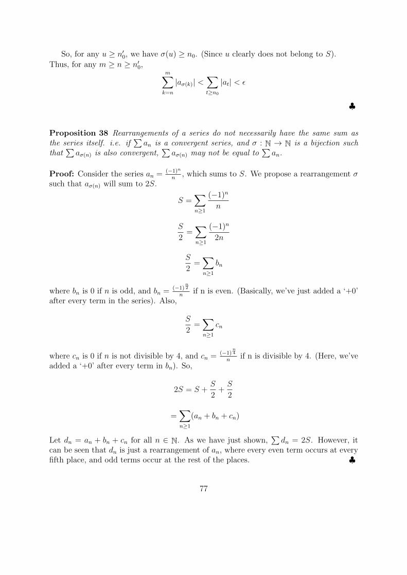
So, for any u ≥ n′0, we have σ(u) ≥ n0. (Since u clearly does not belong to S).

Thus, for any m ≥ n ≥ n′0,m∑k=n

|aσ(k)| <∑t≥n0

|at| < ε

♣

Proposition 38 Rearrangements of a series do not necessarily have the same sum asthe series itself. i.e. if

∑an is a convergent series, and σ : N → N is a bijection such

that∑aσ(n) is also convergent,

∑aσ(n) may not be equal to

∑an.

Proof: Consider the series an = (−1)n

n, which sums to S. We propose a rearrangement σ

such that aσ(n) will sum to 2S.

S =∑n≥1

(−1)n

n

S

2=∑n≥1

(−1)n

2n

S

2=∑n≥1

bn

where bn is 0 if n is odd, and bn = (−1)n2

nif n is even. (Basically, we’ve just added a ‘+0’

after every term in the series). Also,

S

2=∑n≥1

cn

where cn is 0 if n is not divisible by 4, and cn = (−1)n4

nif n is divisible by 4. (Here, we’ve

added a ‘+0’ after every term in bn). So,

2S = S +S

2+S

2

=∑n≥1

(an + bn + cn)

Let dn = an + bn + cn for all n ∈ N. As we have just shown,∑dn = 2S. However, it

can be seen that dn is just a rearrangement of an, where every even term occurs at everyfifth place, and odd terms occur at the rest of the places. ♣

77

3.3.1 Power Series

Definition 48 (Radius of Convergence) Given a series∑

n≥0 anxn , its radius of

convergence is defined to be

R =1

lim supn→∞

n√|an|

Theorem 45 Suppose f(x) =∑n≥0

anxn has radius of convergence R > 0, then

1. g(x) =∑

n≥1 nanxn−1 also has radius of convergence R.

2. f is differentiable on (R,R) and f ′(x) = g(x) for all x ∈ (−R,R).

Proof:Part 1:The radius of convergence of this series is

1

lim supn→∞

n√|an+1|(n+ 1)

=1

lim supn→∞

n√|an+1|

1

lim supn→∞

n√n+ 1

= R · 1

= R.

Part 2:Pick a certain x ∈ (−R,R)

We need to show that for every ε > 0 there exists a δ > 0 such that |f(x)−f(t)x−t − g(x)| < ε

provided |x− t| < δ; that is, as x→ t we have |f(x)−f(t)x−t − g(x)| → 0

Without loss of generality, we can assume x < t < β < R

|f(x)− f(t)

x− t− g(x)| = |

∑n≥1

an(xn − tn

x− t− nxn−1)|

= |∑n≥1

an[(xn−1 + txn−2 + t2xn−3 + ...+ tn−1)− nxn−1]|

=∑n≥1

|an||(xn−1 − xn−1) + (txn−2 − xn−1) + ...+ (tn−1 − xn−1)|

=∑n≥1

|an||xn−2(t− x) + ...+ xn−r−1(tr − xr) + ...+ (tn−1 − xn−1)|

=∑n≥1

|an||(t− x)[xn−2 + xn−3(t+ x) + ...+ (tn−2 + tn−3x+ ...+ xn−2)]|

78

≤∑n≥1

|an||t− x|n(n− 1)

2βn−2

=|t− x|β2

(∑n≥1

|an|n(n− 1)

2βn)

Since β < R, the root test, tells us that

lim supn

√|an|

n(n− 1)

2=

1

R· 1 =

1

R,

and we have

|f(x)− f(t)

x− t− g(x)| ≤ |x− t|

β2(∑n≥1

|an|n(n− 1)

2βn).

Thus as x→ t or |x− t| → 0,

|f(x)− f(t)

x− t− g(x)| → 0.

♣

Corollary 6 A function defined by a power series f(x) =∑

n≥0 anxn is infinitely often

differentiable, and the derivatives can be computed by differentiating the series term-by-term.

In particular, we recall some ‘well-known’ functions’ from elementary calculus; here aretheir formal definitions!

Definition 49 •ex :=

∑n≥0

xn

n!.

•cos(x) :=

∑n≥0

(−1)n

(2n)!x2n.

•sin(x) :=

∑n≥0

(−1)n

(2n+ 1)!x2n+1.

By the theorem above,

• (ex)′ = ex.

• (sin(x))′ = cos(x).

• (cos(x))′ = sin(x).

79

Consider f(x) =∑

n≥0 anxn, then on differentiating it repeatedly we obtain

f(0) = a0, f′(0) = a1,

f ′′(0)

2!= a2,

f ′′′(0)

3!= a3

and so on. In general,

an =f (n)(0)

n!

In short, if f has a power series in some neighborhood of 0, then power series expansionfor f can be uniquely determined.

If we are given a function f , can we determine if it has a power series expansion?Suppose f has derivatives of all order, the candidate for the power series of f is

f(x) =∑n≥0

f (n)(0)

n!xn

Definition 50 A function is said to be analytic on an open interval I, if

f(x) =∑n≥0

an(x− α)n

which holds for all x ∈ I, for some α ∈ I.

NOTE: The expansion∑

n≥0f (n)(0)n!

xn is called the TAYLOR SERIES for f .

Definition 51 A function is said to be smooth if all its derivatives exist.

FACT: There exist smooth and non-analytic functions defined on R.

3.3.2 Taylor Series and Taylor Approximation

Theorem 46 (Taylor Approximation)Suppose f (i)(x) exists for all x ∈ (a, b) and 0 ≤ i ≤ r for some r ∈ N.Define R(h) = f(x+ h)− PTaylor(h) where,

PTaylor(h) =r∑

k=0

f (k)(x)

k!hk

Then,

limh→0

R(h)

hr= 0.

80

Proof:Suppose h > 0Now we have R(0) = R′(0) = R′′(0) = ... = R(r)(0) = 0.Thus by the mean value theorem, we have a θ1 where 0 ≤ θ1 ≤ h such that,

R(h) = R(h)−R(0) = R′(θ1)h

Similarly we will have,

R′(θ1) = R′(θ1)−R′(0) = R′′(θ2)θ1

R′′(θ2) = R′′(θ2)−R′′(0) = R′′′(θ3)θ2

...

R(r−2)(θr−2) = R(r−2)(θr−2)−R(r−2)(0) = R(r−1)(θr−1)θr−2

where, h ≥ θ1 ≥ θ2 ≥ ... ≥ θr−1 ≥ 0 .

|R(h)

hr| = |R

′(θ1)h

hr| = ... = |θ1θ2...θr−2hR

(r−1)(θr−1)

hr| = |θ1

h

θ2

h...θr−2

h

R(r−1)(θr−1)

h|

Since we have h ≥ θ1 ≥ θ2 ≥ ... ≥ θr−1 ≥ 0, so each θih

will be less than 1. Thus,

|R(h)

hr| ≤ |R

(r−1)θrh

| ≤ |R(r−1)(θr−1)

θr−1

| = |R(r−1)(θr−1)−R(r−1)(0)

θr−1

|

Now, as h→ 0, we also have θr−1 → 0. So,

limh→0|R(h)

hr| = lim

h→0|R

(r−1)(θr−1)−R(r−1)(0)

θr−1

| = limθr−1→0

|R(r−1)(θr−1)−R(r−1)(0)

θr−1

| = |R(r)(0)| = 0

Therefore,

limh→0

R(h)

hr= 0.

♣

Theorem 47 Suppose in addition to the hypothesis of the above theorem, we also havethat f (r+1)(x) exists, that is f (i)(x) exists for all x ∈ (a, b) and 0 ≤ i ≤ r + 1, then

R(h) =f (r+1)(θ)

(r + 1)!hr+1,

for some θ ∈ (x, x+ h).

81

Proof:Suppose h > 0. Consider for 0 ≤ t ≤ h

g(t) = f(x+ t)−r∑

k=0

(f (k)(x)

k!tk)− R(h)

hr+1tr+1

Now we have g(0) = g′(0) = ... = g(r)(0) = 0. So using the mean value theorem, we getg(0) = 0 and g(h) = 0 ⇒ there exists θ1, 0 ≤ θ1 ≤ h such that g′(θ1) = 0Hence there exists θ2, 0 ≤ θ1 ≤ θ1 such that g′′(θ2) = 0Continuing in this vein, we see that there exists θr, 0 ≤ θr ≤ θr−1 such that g(r)(θr) = 0.

Also g(r) is differentiable, so,

g(r+1)(t) = f (r+1)(x+ t)− R(h)

hr+1(r + 1)!

Since g(r)(0) = g(r)(θr) = 0, by mean value theorem, there exists θr+1 ∈ (0, θr) such that

g(r+1)(θr+1) = 0

⇒ f (r+1)(x+ θr+1)− R(h)

hr+1(r + 1)! = 0

Thus for θ = x+ θr+1, we have θ ∈ (x, x+ θr) ⊆ (x, x+ h) such that

f (r+1)(θ)− R(h)

hr+1(r + 1)! = 0

⇒ R(h) =f (r+1)(θ)

(r + 1)!hr+1

♣

3.4 Uniform Convergence

Definition 52 A sequence fn is said to converge uniformly to f on [0, 1] if givenε > 0, there exists n0 ∈ N such that |fn(x)− f(x)| < ε whenever n ≥ n0 for all x ∈ [0, 1].This is denoted by writing fn ⇒ f .

Theorem 48 Suppose fn : [0, 1] → R and fn ⇒ f on [0, 1]. If fn are continuous at x0

for some x0 ∈ [0, 1], then f is also continuous at x0.

Proof:Given an ε > 0, we have to show that there exists δ > 0 such that |x0 − x| < δ ⇒|f(x0)− f(x)| < ε.

82

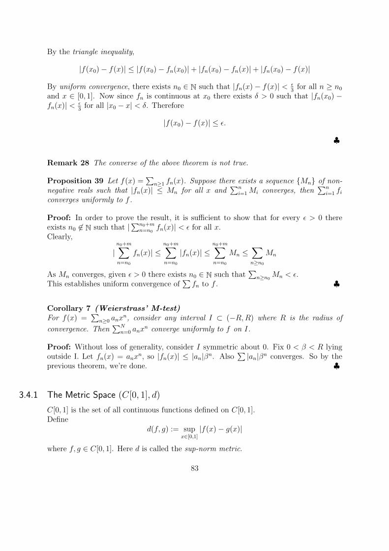
By the triangle inequality,

|f(x0)− f(x)| ≤ |f(x0)− fn(x0)|+ |fn(x0)− fn(x)|+ |fn(x0)− f(x)|

By uniform convergence, there exists n0 ∈ N such that |fn(x)− f(x)| < ε3

for all n ≥ n0

and x ∈ [0, 1]. Now since fn is continuous at x0 there exists δ > 0 such that |fn(x0) −fn(x)| < ε

3for all |x0 − x| < δ. Therefore

|f(x0)− f(x)| ≤ ε.

♣

Remark 28 The converse of the above theorem is not true.

Proposition 39 Let f(x) =∑

n≥1 fn(x). Suppose there exists a sequence Mn of non-negative reals such that |fn(x)| ≤ Mn for all x and

∑ni=1Mi converges, then

∑ni=1 fi

converges uniformly to f .

Proof: In order to prove the result, it is sufficient to show that for every ε > 0 thereexists n0 6∈ N such that |

∑n0+mn=n0

fn(x)| < ε for all x.Clearly,

|n0+m∑n=n0

fn(x)| ≤n0+m∑n=n0

|fn(x)| ≤n0+m∑n=n0

Mn ≤∑n≥n0

Mn

As Mn converges, given ε > 0 there exists n0 ∈ N such that∑

n≥n0Mn < ε.

This establishes uniform convergence of∑fn to f . ♣

Corollary 7 (Weierstrass’ M-test)For f(x) =

∑n≥0 anx

n, consider any interval I ⊂ (−R,R) where R is the radius of

convergence. Then∑N

n=0 anxn converge uniformly to f on I.

Proof: Without loss of generality, consider I symmetric about 0. Fix 0 < β < R lyingoutside I. Let fn(x) = anx

n, so |fn(x)| ≤ |an|βn. Also∑|an|βn converges. So by the

previous theorem, we’re done. ♣

3.4.1 The Metric Space (C[0, 1], d)

C[0, 1] is the set of all continuous functions defined on C[0, 1].Define

d(f, g) := supx∈[0,1]

|f(x)− g(x)|

where f, g ∈ C[0, 1]. Here d is called the sup-norm metric.

83

Proposition 40 (C[0, 1], d) is a metric space.

Proof:

d(f, g) := supx∈[0,1]

|f(x)− g(x)|

where f, g ∈ C[0, 1]. Clearly,d(f, f) = 0

and,d(f, g) = 0⇔ f(x) = g(x) for all x ∈ [0, 1]

Now,d(f, h) = sup

x∈[0,1]

|f(x)− h(x)| = supx∈[0,1]

|f(x)− g(x) + g(x)− h(x)|.

Hence,

d(f, h) ≤ supx∈[0,1]

(|f(x)− g(x)|+ |g(x)− h(x)|)

≤ supx∈[0,1]

|f(x)− g(x)|+ supx∈[0,1]

|g(x)− h(x)|

= d(f, g) + d(g, h).

This proves the result. ♣

Remark 29 Define‖ f ‖sup:= sup

x∈[0,1]

|f(x)|.

So the corresponding distance d(f, g) =‖ f − g ‖sup.

Remark 30 Since C[0, 1] is a metric space, fn ⇒ f ⇔ d(fn, f)→ 0 as n→∞.

Theorem 49 C[0, 1] is complete with respect to the sup-norm metric.

Proof:Suppose fn is Cauchy in C[0, 1] with respect to the sup-norm metric.Given an ε > 0, we have to find an n0 such that |fn(x) − f(x)| ≤ ε, for all x ∈ [0, 1],whenever n ≥ n0.Since fn is Cauchy, we can find an n0 such that

supx∈[0,1]

|fn(x)− fm(x)| < ε

2

whenever m,n ≥ n0.

84

So, for each fixed x ∈ [0, 1], fn(x) is a real Cauchy sequence. Define

f(x) := limn→∞

fn(x)

Now, for any x ∈ [0, 1], take Mx such that

|fm(x)− f(x)| ≤ ε

2

for all m ≥Mx.Now, for any n ≥ n0,

|fn(x)− f(x)| ≤ |fn(x)− fMx(x)|+ |fMx(x)− f(x)| ≤ ε

2+ε

2.

♣

3.4.2 Theorems of Weierstrass

Theorem 50 (Weierstrass’ Approximation Theorem)Suppose f ∈ C[0, 1] and ε > 0. There is a polynomial P ∈ C[0, 1] such that ‖ f−P ‖sup<ε. In other words, if P denotes the set of polynomials in C[0, 1], then P is dense inC[0, 1].

Proof:(Bernstein)f ∈ C[0, 1] ⇒ given ε > 0 there exists δ > 0 such that |f(x) − f(y)| < ε whenever|x− y| < δ.Let ‖ f ‖sup= M . Consider

P (x) =n∑k=0

(n

k

)xk(1− x)n−kf(

k

n)

|f(x)− P (x)| = |(x+ 1− x)nf(x)− P (x)|

= |n∑k=0

(n

k

)xk(1− x)n−k(f(x)− f(

k

n))|

Suppose X is a random variable X ∼ Bin(n, x). Then(n

k

)xk(1− x)n−k = P (X = k)

By Chebychev’s inequality,

P (|X − nx| > t) ≤ nx(1− x)

t2≤ n

4t2

85

Taking t = n23 ,

P (|X − nx| > t) ≤ 1

4n13

Call k as deviant if |k − nx| > n23 . So,∑

deviant k

(n

k

)xk(1− x)n−k <

1

4n13

⇒ |n∑k=0

(n

k

)xk(1− x)n−k(f(x)− f(

k

n))|

≤∑

deviant k

(n

k

)xk(1−x)n−k|(f(x)−f(

k

n))|+

∑non−deviant k

(n

k

)xk(1−x)n−k|(f(x)−f(

k

n))|

Now, ∑deviant k

(n

k

)xk(1− x)n−k|(f(x)− f(

k

n))| ≤ 2M

4n13

and, ∑non−deviant k

(n

k

)xk(1− x)n−k|(f(x)− f(

k

n))|

≤ (∑

non−deviant k

(n

k

)xk(1− x)n−k) ( sup

non−deviant k|f(x)− f(

k

n)|)

< supnon−deviant k

|f(x)− f(k

n)|

Pick δ > 0 such that |f(x)− f(y)| < ε2

whenever |x− y| < δ and pick n such that n13 > 2

δ

and M

2n13< ε

2.

This will guarantee that P is the required polynomial. ♣

Theorem 51 (Weirstrass)There exists f : R→ R such that f is continuous but nowhere differentiable.

Proof: Let f0(x) : R→ R

f0(x) =

(x) on [2n, 2n+ 1]

(1− x) on [2n+ 1, 2n+ 2]∀n ∈ Z

and fk(x) = αkf0(4kx), for some 0 < α < 1.

Let f(x) =∑

k≥0 fk(x)

Since ||fk|| ≤ αk and∑

k≥0 αk <∞, by the M-test it follows that f is continuous.

86

Claim 16 f is any NOT differentiable at any x ∈ R.

Observe : ‘Slopes’ appearing on f0 ∈ 1,−1.‘Slopes’ appearing on fk ∈ (4α)k,−(4α)k.So we want α > 1

4but α < 1 (if f can be guaranteed to be non-differentiable).

It suffices to show that there is a sequence δn → 0(δn ≥ 0) such that

|f(x± δn)− f(x)

δn| ≥ n

Also notice that f0(x+ 2) = f0(x) for all x.

fk(x+2

4k) = αkf0(4k(x+

2

4k))

= αkf0(4kx+ 2)

= αkf0(4kx)

= fk(x)

Choose δn = 12(4n)

f(x± δn)− f(x)

δn=∑k≥0

αkf0(4k(x± δn))− f0(4kx)

δn.

For k > n, coefficients are zero, therefore

f(x± δn)− f(x)

δn=

n∑k≥0

αkf0(4k(x± δn))− f0(4kx)

δn.

At k = n , αkf0(4kx± 12

)−f0(4kx)

δn = (4α)k.

For k < n,

αkf0(4k(x± 1

2.4n))− f0(4kx)

12.4n

≤ (4α)k,

|f(x± δn)− f(x)

δn| = |

∑k<n

fk(x± δn)− f(x)

δn± (4α)n| ≥ (4α)n −

∑0≤k<n

(4α)k.

Now,n−1∑

0

(4α)k =(4α)n − 1

4α− 1,

so

(4α)n − ((4α)n − 1

4α− 1) > (

4α− 2

4α− 1).(4α)n.

87

This shows that f ′(x) → ∞ as n → ∞. As x was arbitrary, this shows that f ′(x) doesnot exist for any x ∈ R. ♣

We denote C[a, b] as the set of continuous functions in the interval [a, b]. The previousresult in fact shows that there are members of C[0, 1] that are nowhere differentiable in[a, b].

One might wonder if the example of Weierstrass is a pathological extreme, and is notthe norm. The next result however shows that far from being the norm, most members ofC[a, b] are in fact of this type, i.e., a ‘generic’ element of C[a, b] is nowhere differentiable.

Theorem 52 Consider f ∈ C[0, 1]. A ‘generic’ element of C[0, 1] is nowhere differen-tiable.

Consider for some hn,x > 0,

Rn =

f ∈ C[0, 1]

∣∣∣∣|f(x± hn,x)− f(x)

hn,x| ≥ n ∀x ∈ [0, 1− 1

n]

Note that if f is differentiable at x ∈ (0, 1), then f /∈ Rn for all n ≥ n0 for some n0 ∈ N.If f ∈

⋂n≥1Rn, then f is nowhere differentiable (not differentiable at every x ∈ [0, 1] ).

We shall first prove a lemma.

Lemma 9 Define Rn as,

Rn := f ∈ C[0, 1]

∣∣∣∣|f(x± hn,x)− f(x)

hn,x| ≥ n ∀x ∈ [0, 1− 1

n].

Then Rn is open and dense in C[0, 1].

Note 3 In general, in a metric space (X , d) if Un ⊂ X , are open in X , then one couldhave

⋂n≥1 Un = ∅.

The theorem follows as a consequence of the Baire Category theorem, which we shall doin the next section, and the lemma above. This incidentally also defines what we meanby ‘generic’.

Proof: There are two things we need to prove:

1. Rn is open in C[0, 1].

2. Rn is dense in C[0, 1].

We will address both of these below.

88

1. We have to show that, given f ∈ Rn we want ε > 0 such that for all g ∈ C [0, 1]satisfying ‖f − g‖sup < ε we also have g ∈ Rn.

For each x, there is a hx = h such that

|f(x± h)− f(x)

h| > n.

The functions f(x±h)−f(x)h

are continuous and have absolute value greater than n atx.

By continuity, there is some small interval Ix containing x and a δx > 0 such that|f(y±hx)−f(y)

hx| ≥ n+ δx for all y ∈ Ix and corresponding hx for an appropriate choice

of + or −.

Consider

U =

Ix | x ∈

[0, 1− 1

n

].

This clearly covers[0, 1− 1

n

]. So by compactness of

[0, 1− 1

n

], there is a finite

sub-cover, i.e., there exist x1, x2 . . . . . . xr such that⋃ri=1 Ixi covers

[0, 1− 1

n

]. In

other words, for all x ∈[0, 1− 1

n

], |f(x±h)−f(x)

h| > n+ min δ1, δ2, ...δr

and a suitable h for each x.

In particular, if ‖g − f‖ < ε, then

|g(x+ h)− g(x)

h−f(x+ h)− f(x)

h| = |(g(x+ h)− f(x+ h))− (g (x)− f (x))

h| ≥ n.

This completes the proof.

2. We have to show that, given f ∈ C [0, 1] and ε > 0, we want a g ∈ Rn and‖g − f‖ < ε. We shall think of g = f + a where h satisfies ‖a‖ < ε, where a is asuitable sawtooth function.

|f(x+ h) + a(x+ h)− f (x)− a (x)

h| > n

= |f(x+ h)− f(x)

h− a(x+ h)− a(x)

h|

a (x) =

(3

4

)kfo(4kx),

for a large enough k.

So slopes occurring in a are ±3k.

If f is piecewise linear, then f consists of finite number of straight line segments.

89

Let M = max(slopes of line segments occurring in f). Pick k large so that 3k−M >n and we are through.

If P ∈ C [0, 1] is the set of all piecewise linear functions in C [0, 1], then (Rn

⋂P )

is dense in P .

Hence, P is dense in C [0, 1] and therefore Rn is dense in C [0, 1]. This completesthe proof of the lemma.

♣

3.4.3 Baire Category Theorem

In this section, we state and prove the Baire Category theorem (in the context of aComplete Metric space) which completes the proof of the previous theorem. It statesthat in a complete metric space, dense open sets are in some sense, ‘large’. This sense oflargeness is not set-theoretic (i.e., in cardinality terms) but is something topological.

Theorem 53 (Baire Category Theorem)In a complete metric space (X , d), if Un ⊂ X are open and dense, then

⋂n Un is dense in

X .

Proof: Let x ∈ X and let ε > 0. U1 is dense and open, so there exists P1 ∈ Bε (x) andr1 > 0 such that

Br1 (P1) ⊂ Bε (x)⋂

U1.

U2 is open and dense. So there exists P2 and r2 such that Br2 (p2) ⊂ Br1 (p1)⋂U2 ⊆

U1

⋂U2.

Get Pn ∈ X , rn ∈ R such that Brn(Pn) ⊂ Brn−1(Pn−1)⋂Un for each n ≥ 2.

Consider Pn. Note that Brn(Pn) contains Pm for all m ≥ n. rn can be chosen asrn <

rn−1

2. So rn <

ε2n−1 if m, k ≥ n, so Pn is Cauchy. Since X is complete, Pn → p for

some p.

Claim 17 p ∈ Un for all n ∈ N.

Note that: d(p, x) < 2ε. So, d(p, x) ≤ d(x, px) + d(px, p). Pick ` such that d(p`, p) <ε4.

d(x, p`) < ε so d(p, x) < 2ε.We want to show that p ∈ Un for all n; that will complete the proof. To see for instancethat p ∈ U1, note that

Pn ∈ Br2 (P2) ⊂ U1

for all n ≥ 2. Hence, p ∈ U1 since p is a limit point of Pn. Similarly we can show thatp ∈ Un for all n ∈ N. ♣

90

Remark 31 As commented before, the last lemma of the previous section and the Bairecategory theorem tell us that functions that are nowhere differentiable are in fact densein C[0, 1].

Definition 53 A set A is of CATEGORY 1 if A can be written as countable union of“nowhere dense” sets.

(A set A is nowhere dense if A does not contain any non-trivial open ball.)

Examples :

1. X = R and A is any linear set.

2. X = R A = Z.

3. X = R A = Q.

Definition 54 A set is said to be of CATEGORY 2 if it is not CATEGORY 1.

Proposition 41 Suppose X is a metric space. The following are equivalent.

• X is CATEGORY 2.

• Un ⊂ X are dense open ⇒⋂n Un is dense in X .

Examples:

1. Cantor set is of category 1.

2. Real line(R) is of category 2.

91

4 Riemann Integration

4.1 Integrals according to Riemann and Darboux

Definition 55 A Partition P of [a, b] is a set

a = x0 < x1 < x2 < · · · < xn = b

Definition 56 For a bounded function f , let

mi = infx∈[xi−1,xi]

f(x)

where i = 1, 2, ..., n. Then the Lower Sum denoted by L(P, f) is given by

L(P, f) :=n∑i=1

mi(xi − xi−1).

Definition 57 For a bounded function f , let

Mi = supx∈[xi−1,xi]

f(x)

where i = 1, 2, ..., n. Then the Upper Sum denoted by U(P, f) is given by

U(P, f) :=n∑i=1

Mi(xi − xi−1).

Definition 58 A partition Q is a refinement of P if Q ⊇ P and this is denoted byQ P .

Observations:

1. If Q P ,then U(Q, f) ≤ U(P, f).

Proof: The case where Q = P is trivial. Otherwise, Q contains some additionalpoints to that of P . As they must belong to some interval of P ,let us denote themas yi ∈ [xi−1, xi]. Now

Mi = sup[xi−1,xi]

f(x) ≥ Mi(1) = sup

[xi−1,yi]

f(x) (4.1)

Mi = sup[xi−1,xi]

f(x) ≥ Mi(2) = sup

[yi,xi]

f(x). (4.2)

93

Hence,

Mi(xi − xi−1) = Mi(xi − yi) +Mi(yi − xi−1) ≥Mi(2)(xi − yi) +Mi

(1)(yi − xi−1).

Therefore

U(Q, f) ≤ U(P, f).

2. If Q P ,then L(Q, f) ≥ L(P, f).

Proof of this is similar to the above case except for Mi being replaced with mi andthe inequalities reversed.

Definition 59 For a partition P ,the Norm of P (written as N (P )) equals

maxxi − xi−1|1 ≤ i ≤ n.

Definition 60 Darboux Integrability: We say f : [a, b]→ R is (Darboux) integrableif there exists a real I such that the following holds: Given ε > 0, there exists δ > 0 suchthat for any partition P with N (P ) < δ,we have

|U(P, f)− I| < ε and |I − L(P, f)| < ε.

Observe that f is Darboux integrable iff given ε > 0, there exists δ >0 such that

for every P with N (P ) < δ, we have

U(P, f) < L(P, f) + ε.

This is because both U(P, f) and L(P, f) tend to the same I as N (P ) tends to zero.

Definition 61 Riemann Integrability: Given P , let T be a subset of [a, b] such that

T = t1 ≤ t2 ≤ ... ≤ tn and ti ∈ [xi−1, xi]

Define

R(P, T, f) =n∑i=1

(xi − xi−1).f(ti).

f is (Riemann) integrable if there exists I real such that

given ε > 0, there exists δ > 0 such that for any P with N (P ) < δ and any T of P ,

|R(P, T, f)− I| < ε.

The above sum R(P, T, f) is called Riemann sum of f w.r.t partition P .

Theorem 54 Darboux integrability is equivalent to Riemann integrability.

94

Proof: Darboux integrability ⇒ Riemann integrability:

mi ≤ f(ti) ≤Mi for every ti ∈ [xi−1, xi].Therefore

mi(xi − xi−1) ≤ f(ti)(xi − xi−1) ≤Mi(xi − xi−1) (4.3)

L(P, f) ≤ R(P, T, f) ≤ U(P, f) (4.4)

By Darboux integrability, we mean that both L(P, f), U(P, f) tend to I as N (P ) tends tozero. From (3),(4), by the Sandwich Theorem, R(P, T, f) tends to I which is equivalentto

|R(P, T, f)− I| < ε.

Riemann integrability ⇒ Darboux integrability:

Riemann integrability provides us a P such that |R(P, T, f)− I| < ε

2for every T

of P . Choose T1 = t11 ≤ t21 ≤ ... ≤ tn1 such that for every ti1 ∈ [xi−1, xi],

f(ti1) +ε

2(b− a)> sup

[xi−1,xi]

f(x).

Then

U(P, f)−R(P, T1, f) <ε

2(b− a)

n∑i=1

(xi − xi−1) =ε

2

Similarly,choose T2 = t12 ≤ t22 ≤ ... ≤ tn2 such that for every ti2 ∈ [xi−1, xi],

f(ti2)−ε

2(b− a)< inf

[xi−1,xi]f(x)

Then

R(P, T2, f)− L(P, f) >ε

2

Hence,by Triangle inequality, we have |U(P, f)− I| < ε and |I − L(P, f)| < ε. ♣

Notation 1: We define the set R[a, b] to denote the set of all Riemann integrable func-tions on [a, b].

Proposition 42 If f is continuous on [a, b], then f is integrable on [a, b], i.e., f ∈C[a, b]⇒ f ∈ R[a, b].

Proof: Given ε > 0, we need to show that U(P, f) − L(P, f) < ε for N (P ) < δ. Giventhat f is continuous on [a, b], it follows that f is uniformly continuous on [a, b], i.e., givenε > 0, there exists δ > 0 such that

|x− y| < δ ⇒ |f(x)− f(y)| < ε.

95

Here,ε

b− ais also another positive number. Hence ε can be replaced by

ε

b− a.

For any partition P with N (P ) < δ, we have

maxx∈[xi−1,xi]

f(x)− minx∈[xi−1,xi]

f(x) <ε

b− a.

U(P, f)− L(P, f) =n∑i=1

(Mi −mi)(xi − xi−1) <ε

b− a

n∑i=1

(xi − xi−1) =ε

b− a(b− a) = ε.

This completes the proof. ♣

Example 15

f(x) =

1 : x ∈ [0, 1]0 : x ∈ (1, 2]

This is also Riemann integrable. To see this, note that for a partition P , any interval ofP does not contain x = 1,we are through. Else, as the norm of P gets lower and lower,it essentially adds to zero and hence is Riemann integrable.

Example 16

f(x) =

1 : x ∈ Q0 : x /∈ Q

Mi on any subinterval is 1 and mi on any subinterval is 0. Hence U(P, f) does not tendto

L(P, f) for any partition. This is therefore not Riemann integrable.

What kind of discontinuities admit Riemann Integrability? Before answering this

question,we’ll look into the concept of measure zero.

4.2 Measure Zero sets and Riemann Integrability

Concept of Measure Zero: A set A is said to be of Measure Zero if given ε > 0,

there exists a sequence of open intervals (ai, bi)i≥1 such that⋃i≥1

(ai, bi) covers A and∑i

(bi − ai) < ε.

Examples:

1. Finite sets.

2. Countable sets.

3. Cantor set.

96

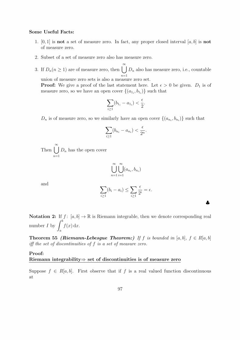
Some Useful Facts:

1. [0, 1] is not a set of measure zero. In fact, any proper closed interval [a, b] is notof measure zero.

2. Subset of a set of measure zero also has measure zero.

3. If Dn(n ≥ 1) are of measure zero, then∞⋃n=1

Dn also has measure zero, i.e., countable

union of measure zero sets is also a measure zero set.Proof: We give a proof of the last statement here. Let ε > 0 be given. D1 is ofmeasure zero, so we have an open cover (a1i , b1i) such that∑

i≥1

(b1i − a1i) <ε

2.

Dn is of measure zero, so we similarly have an open cover (ani , bni) such that∑i≥1

(bni − ani) <ε

2n.

Then∞⋃n=1

Dn has the open cover

∞⋃n=1

∞⋃i=1

(ani , bni)

and ∑i≥1

(bi − ai) ≤∑i≥1

ε

2i= ε.

♣

Notation 2: If f : [a, b]→ R is Riemann integrable, then we denote corresponding real

number I by

∫ b

a

f(x) dx.

Theorem 55 (Riemann-Lebesgue Theorem:) If f is bounded in [a, b], f ∈ R[a, b]iff the set of discontinuities of f is a set of measure zero.

Proof:Riemann integrability⇒ set of discontinuities is of measure zero

Suppose f ∈ R[a, b]. First observe that if f is a real valued function discontinuousat

97

x0, then there exists ε > 0 such that

supy∈(x−r,x+r)

f(y)− infy∈(x−r,x+r)

f(y) ≥ ε

for every r ≥ 0, i.e.,

oscf (x) := limr→0

diam(f(x− r, x+ r)) ≥ ε.

Fact: f is discontinuous at x if and only if oscf (x) > 0.

Let D(f) be the set of discontinuities of f . Then D(f) =⋃n≥1

Df (n) where

Df (n) = x : oscf (x) ≥ 1

n.

So, if f ∈ R[a, b], it suffices to show that for each n ≥ 1, Df (n) has measure zero. Asf ∈ R[a, b], given ε > 0, there exists δ > 0 such that for P satisfying N (P ) < δ, we have

U(P, f)− L(P, f) <ε

n.

In particular, take the open intervals (xi, xi+1) determined by the partition P such that

Df (n) ⊂⋃i

(xi, xi+1); call i BAD if (xi, xi+1) ∩Df (n) 6= ∅. Therefore,

∑i

(xi+1 − xi)n

≤∑BADi

(Mi −mi)(xi+1 − xi) ≤ U(P, f)− L(P, f) <ε

n∑i

(xi+1 − xi) < ε.

Hence, Df (n) is of measure zero. Hence⋃n≥1

Df (n), a countable union of measure zero

sets, is also of measure zero.

Proof of Converse:

Given Df has measure zero. Note that if x ∈ Df \ Df (n), then oscf (x) <1

n. Consider

D1 =n⋃i=1

Df (i) for some large n (which will be determined later) and D2 = Df \D1.

Now D1 =n⋃i=1

Df (i) is a set of measure zero. So, there’s a collection of open intervals

(ai, bi) such that D1 ⊆⋃i

(ai, bi) and∑i

(bi − ai) < ε for any ε > 0.

We want a δ > 0 such that any P with N (P ) < δ satisfies U(P, f)− L(P, f) < ε. Note

98

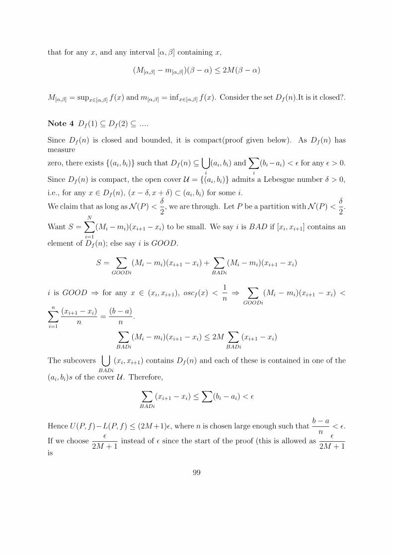
that for any x, and any interval [α, β] containing x,

(M[α,β] −m[α,β])(β − α) ≤ 2M(β − α)

M[α,β] = supx∈[α,β] f(x) and m[α,β] = infx∈[α,β] f(x). Consider the set Df (n).It is it closed?.

Note 4 Df (1) ⊆ Df (2) ⊆ ....

Since Df (n) is closed and bounded, it is compact(proof given below). As Df (n) hasmeasure

zero, there exists (ai, bi) such that Df (n) ⊆⋃i

(ai, bi) and∑i

(bi−ai) < ε for any ε > 0.

Since Df (n) is compact, the open cover U = (ai, bi) admits a Lebesgue number δ > 0,

i.e., for any x ∈ Df (n), (x− δ, x+ δ) ⊂ (ai, bi) for some i.

We claim that as long asN (P ) <δ

2, we are through. Let P be a partition withN (P ) <

δ

2.

Want S =N∑i=1

(Mi−mi)(xi+1− xi) to be small. We say i is BAD if [xi, xi+1] contains an

element of Df (n); else say i is GOOD.

S =∑

GOODi

(Mi −mi)(xi+1 − xi) +∑BADi

(Mi −mi)(xi+1 − xi)

i is GOOD ⇒ for any x ∈ (xi, xi+1), oscf (x) <1

n⇒

∑GOODi

(Mi − mi)(xi+1 − xi) <

n∑i=1

(xi+1 − xi)n

=(b− a)

n.∑

BADi

(Mi −mi)(xi+1 − xi) ≤ 2M∑BADi

(xi+1 − xi)

The subcovers⋃BADi

(xi, xi+1) contains Df (n) and each of these is contained in one of the

(ai, bi)s of the cover U . Therefore,∑BADi

(xi+1 − xi) ≤∑

(bi − ai) < ε

Hence U(P, f)−L(P, f) ≤ (2M+1)ε, where n is chosen large enough such thatb− an

< ε.

If we chooseε

2M + 1instead of ε since the start of the proof (this is allowed as

ε

2M + 1is

99

also another positive number), we end up getting

U(P, f)− L(P, f) ≤ ε

♣

Proposition 43 Let f have the domain [a, b]. Then for any n, Dn(f) = x ∈ [a, b] such

that oscf (x) ≥ 1

n is compact.

Proof: Our claim is that Dnc is open in [a, b]. For every x0 ∈ Dn

c,oscf (x0) = t(say)<1

n.

So,t = lim

h→0sup |f(x1)− f(x2)|

for x1, x2 ∈ (x0 − h, x0 + h) ∩ [a, b].Therefore, for ε =1− nt

2n> 0 there exists δ > 0 such

that if 0 < h < δ, then,| sup |f(x1)− f(x2)| − t| < ε

for all x1, x2 ∈ (x0 − h, x0 + h) ∩ [a, b].Therefore,

sup |f(x1)− f(x2)| < t+ ε =t

2+

1

2n<

1

2n+

1

2n<

1

n

That is, (x0− δ, x0 + δ)∩ [a, b] ⊂ Df (n)c. Hence, Df (n)c is open in [a, b] and hence Df (n)

is closed.Also Df (n) ⊂ [a, b] is bounded. Hence, it is compact. ♣

4.3 Consequences of the Riemann-Lebesgue Theorem

1. If f ∈ R[a, b]⋂R[b, c], then f ∈ R[a, c] (a < b < c).

2. f, g ∈ R[a, b]⇒ f ± g ∈ R[a, b] and fg ∈ R[a, b].

3. If g > 0 in [a, b] and g ∈ R[a, b], then1

g∈ R[a, b].

Proposition 44 If f, g ∈ R[a, b],then

1.

∫ b

a

(f + g)(x) dx =

∫ b

a

f(x) dx+

∫ b

a

g(x) dx.

2.

∫ b

a

λf(x) dx = λ

∫ b

a

f(x) dx.

100

3.

∫ b

a

f(x) dx ≤ (sup[a,b]|f |)(b− a).

Proof: (1)f ∈ R[a, b]⇒ we can find a partition P1 such that

U(P1, f)− L(P1, f) <ε

2

Similarly, we can find another partition P2 such that

U(P2, g)− L(P2, g) <ε

2

Now on P = P1 ∪ P2 = a = x0 < x1 < ... < xn = b. supx∈[xi−1,xi](f + g) ≤

supx∈[xi−1,xi]f +

supx∈[xi−1,xi]g and infx∈[xi−1,xi](f + g) ≥ infx∈[xi−1,xi] f + infx∈[xi−1,xi] g. Therefore,

U(P, f + g) ≤ U(P, f) + U(P, g) and −L(P, f + g) ≤ −L(P, f)− L(P, g).Now, P1, P2 ⊆

P .Hence, U(P1, f) ≥ U(P, f) and −L(P1, f) ≥ −L(P, f). Similar thing holds for P2, g.

Now,

U(P, f + g)− L(P, f + g) ≤ U(P, f) + U(P, g)− L(P, f)− L(P, g)

= U(P, f)− L(P, f) + U(P, g)− L(P, g)

≤ U(P1, f)− L(P1, f) + U(P2, g)− L(P2, g)

<ε

2+ε

2= ε

(2),(3) can be similarly proved. ♣

If f ∈ R[a, b], then by Riemann-Lebesgue theorem, [a, b]⋂D(f) is of measure zero ⇒

for any x ∈ (a, b), [a, x]⋂D(f) has measure zero⇒ f ∈ R[a, x] for every x ∈ (a, b].

Consider F (x) =

∫ x

a

f(x) dx ; F (a) = 0 (denoted by

∫ a

a

f(x) dx = 0 for any a.)

Theorem 56 (a) F : [a, b]→ R is continuous.

(b) If f is continuous at x0, then F is differentiable at x0 and F ′(x0) = f(x0)(Fundamental

Theorem of Calculus).

Proof: (a) We need to show that given ε > 0, there exists a δ > 0 such that |x−y| < δ ⇒|F (x)− F (y)| < ε. Without loss of generality, let a < x < y < b.

101

Note 5 If f ∈ R[a, b], f ∈ R[b, c], then f ∈ R[a, c] and∫ c

a

f(x) dx =

∫ b

a

f(x) dx+

∫ c

b

f(x) dx

From the above result,

F (x)− F (y) =

∫ x

y

f(t) dt∣∣∣∣∫ x

y

f(t) dt

∣∣∣∣ ≤ supt∈[x,y]

|f(t)|.(y − x) ≤ supt∈[a,b]

|f(t)|.(y − x) = M.(y − x)

for some M > 0. Therefore,

|F (y)− F (x)| ≤M |y − x|

We can therefore choose δ =ε

Mand this completes the proof of (a).

Now, let h > 0.∣∣∣∣F (x0 + h)− F (x0)

h− f(x0)

∣∣∣∣ =

∣∣∣∣1h∫ x0+h

x0

f(t) dt− f(x0)

∣∣∣∣ =

∣∣∣∣1h∫ x0+h

x0

(f(t)− f(x0)) dt

∣∣∣∣Since f is continuous at x0, given ε > 0, there exists δ > 0 such that for every t ∈(x0, x0 + δ), |f(t)− f(x0)| < ε. ∣∣∣∣∫ b

a

f(t) dt

∣∣∣∣ ≤ ∫ b

a

|f(t)| dt

. Hence, for h < δ∣∣∣∣F (x0 + h)− F (x0)

h− f(x0)

∣∣∣∣ ≤ 1

h

∫ x0+h

x0

|f(t)− f(x0)| dt < ε.h

h= ε

This proves (b). ♣

Note 6 f ′(x) = 0 for every x⇒ f(x) = constant. So, in particular,

f(x) = sin2x+ cos2x⇒ f ′(x) = 2 sinx cosx+ 2 cosx(− sinx) = 0

Therefore f(x)=constant. Plugging x = 0,we get f(x) = 1.

4.4 Antiderivatives and some ‘well known’ Integral Calculus techniques

Definition 62 Given a real valued function f , a real valued function F is an

Antiderivative for f if F is differentiable and F ′ ≡ f .

If F is antiderivative for f , then so is G = F + c where c is any constant.

102

Proposition 45 Any two antiderivatives differ by a constant.

Proof: If F ′ = G′ = f , then (F −G)′ = 0. Hence by note 3, F −G = constant. ♣

Theorem 57 (Integration by Parts) Suppose f , g are differentiable on (a, b) and

continuous on [a, b] and suppose f ′, g′ ∈ R[a, b], then∫ b

a

f ′g(t) dt = fg|ba −∫ b

a

fg′(t) dt.

Proof: By consequences of Riemann-Lebesgue theorem, f ′g, fg′ ∈ R[a, b]. By the

Product rule of differenciation,

(fg)′ = f ′g + fg′ (4.5)

Hence, (fg)′ ∈ R[a, b]. Pick antiderivatives f(x)g(x)−(constant),

∫ x

a

f ′g(t) dt,

∫ x

a

fg′(t) dt

respectively of the three functions in (5) and substitute b for x. Constant can be evalu-ated

by substituting a in x and this yields c = f(a)g(a). This completes the proof. ♣

Theorem 58 (Integration by Substitution) If f ∈ R[α, β], g′ > 0 and continuousfor

every x ∈ [α, β] and g : [a, b] −→ [α, β] bijectively, then∫ b

a

f(g(t))g′(t) dt =

∫ β

α

f(t) dt

Proof: By M.V.T, there exist tis ∈ [xi−1, xi] such that

g(xi)− g(xi−1) = g′(ti)(xi − xi−1)

Pick these tis and form the corresponding Riemann sum

R1(P, T, f) =n∑i=1

f(g(ti))g′(ti)(xi − xi−1) =

n∑i=1

f(g(ti))(g(xi)− g(xi−1))

on [a, b]. Let yi = g(xi) and si = g(ti). Note that as g′(x) > 0, α = y0 < y1 < .... < yn = β

and yi−1 < si < yi. Now, the sum will simplify to R1 =n∑i=1

f(si)(yi − yi−1) which is the

same as the one on the other hand, i.e;∫ β

α

f(t) dt =n∑i=1

f(si)(yi − yi−1) = R1 =

∫ b

a

f(g(t))g′(t) dt.

103

♣

Some facts about sinx and cosx: We know some of the properties of the trigono-metric functions (such as the sin of a sum and so forth); here, we look at some of them,from their formal definitions, and see how we might go about proving them. Recall that

1. cosx =∑n≥0

(−1)nx2n

(2n)!.

sinx =∑n≥0

(−1)nx2n+1

(2n+ 1)!.

Here we consider some well-known properties.

1. Consider f(x) = sin2 x + cos2 x. By differentiating a peer series term-by-term, weknow that (sin x)′ = cosx, (cosx)′ = − sinx. Hence it follows that f ′(x) = 0. By thefundamental theorem of calculus, it follows that f(x) = Const. At x = 0, sinx = 0and cos x = 1, hence this constant is 1. In particular, sin2 x + cos2 x = 1 for all x,and cos x attains its maximum value 1 at x = 0.

2. sin(−x) = − sinx (substituting −x in power series).

3. cos 1 < sin 1.To see this,

sin 1 = 1− 1

3!+

1

5!− 1

7!+ ....

cos 1 = 1− 1

2!+

1

4!− 1

6!+ ....

sin 1− cos 1 =1

2!− 1

3!− 1

4!+

1

5!+

1

6!− 1

7!− 1

8!+ .... =

(1

2!− 1

3!

)−(

1

4!− 1

5!

)+ ....

sin 1− cos 1 =

(2

3!− 4

5!

)+

(6

7!− 8

9!

)+ .....

2n

(2n+ 1)!− 2n+ 2

(2n+ 3)!=

(2n+ 2)(4n2 + 6n− 1)

(2n+ 3)!> 0.

Hence,sin 1 > cos 1.

Define f(x) = cos x− sinx.f(0) = 1 > 0 and f(1) < 0. Therefore by IntermediateValue Property, f(x) = 0 for some x ∈ (0, 1) Hence, there is some x (denoted byπ

4) where sinx = cosx for the first time in (0,∞).

4. Consider the following equations which will be proved later.

sin(x± a) = sinx cos a± cosx sin a (4.6)

cos(x± a) = cos x cos a∓ sinx sin a. (4.7)

104

a) If x = a, then first equation gives us sin 2x = 2 sin x cosx. Plugging x =π

4gives

sin(π

2

)= 2 sin

(π4

)cos(π

4

)= 2 sin2

(π4

).

Butsin2

(π4

)+ cos2

(π4

)= 2 sin2

(π4

)= 1.

hence sin2(π

4

)=

1

2. Therefore, sin

(π2

)= 1.

b) cos2(π

2

)= 1− sin2

(π2

)= 0, so cos

(π2

)= 0.

c) sin(x+

π

2

)= cosx (from eq.n(6))

cos(x+

π

2

)= − sinx.(from eq.n(7))

d) sin(x+ π) = sin(x+

π

2+π

2

)= − sinx

e) sin(x+2π) = sin(x+π+π) = (−1)(−1) sinx = sinx. We can similarly obtaincos(x+ 2π) = cos x. Hence we conclude that sinx and cos x are periodic.

5. To prove that sin(x + a) = sinx cos a + cosx sin a, for instance, consider f(x) =sin(x+a)− sinx cos a−cosx sin a. Then f ′(x) = cos(x+a)−cosx cos a+sinx sin aand f ′′(x) = − sin(x+ a) + sin x cos a+ cosx sin a. Hence f ′′(x) = −f(x).

Note that plugging x = 0 gives f ′(0) = f(0) = 0. Also, f(x) is analytic on Ras sinx, cosx are analytic in R as discussed in the previous chapter. Hence, wecan differentiate it further and obtain the relation f (2n)(x) = (−1)nf(x).Therefore,f (2n)(0) = (−1)nf(0) = 0. Also, f (2n+1)(x) = (−1)nf ′(x). Hence, f (2n+1)(0) =

(−1)nf ′(0) = 0. Hence f(x) =∑n≥1

f (n)(0)xn

n!= 0. Therefore,

sin(x+ a) = sinx. cos a+ cosx. sin a.

By substituting−a for a in the above result we get sin(x−a) = sinx cos a−cosx sin aand differentiating these two results gives cos(x± a) = cos x. cos a∓ sinx sin a.

Some facts about ex and the log function:

1. We have seen that ex =∑n≥0

xn

n!and (ex)′ = ex.Define f(x) = ex.e−x. Hence

f ′(x) = (ex.e−x)′ = ex.e−x + ex.(e−x(−1)) = 0,

so by the fundamental theorem of calculus,

f(x) = c.

105

But f(0) =1. Hence f(x) ≡ 1 for all x. Hence

e−x =1

ex

For x > 0, it is easy to see that ex > 0 (from expansion). Hence e−x > 0. Thisproves that ex is positive throughout and is increasing (Derivative is itself whichis positive⇒ increasing throughout) and hence f has an inverse. We’ll denote itby y = log x. In particular, we have ey = x. Since the inverse of a differentiablefunction is also differentiable, we have (by results of the preceding chapter), thefollowing: If y0 = f(x0),then

(f−1(y0))′ =1

f ′(x0).

In particular, log x is differentiable and

(log x)′ =1

elog x=

1

x.

2. ex+y = exey.This will be proved after the following proposition.

Proposition 46 Suppose g is analytic on R and g′(x) = g(x) for every x, then g(x) =cex for some constant c.

Proof:For every x, we have the following two equations.

g(x) =∑n≥0

g(n)(0)xn

n!(4.8)

g′(x) = g(x) (4.9)

g′(0) = g(0) = c (say). g′′(x) = g′(x) = g(x). Hence g′′(0) = c as well. Proceeding furtherby differentiating the equation g′(x) = g(x), by induction, we obtain that g(n)(0) = c forevery n. Hence, substituting g(n)(0) back in eq.n(8),we get the desired form, i.e.,

g(x) = cex.

♣

Now, consider f(x) = ex+a− ex.ea. f ′(x) = ex+a− ex.ea = f(x) for every x ∈ R and f(x)

is analytic throughout R as discussed in topic 3. Hence by above proposition, f(x) = cex.Substituting x = 0 in this equation, f(0) = c. But f(0) = ea − ea(1) = 0. Hence c = 0and so f(x) ≡ 0.

106

4.5 The Integral Test

Notation: By

∫ ∞a

f(x) dx, we mean limN→∞

∫ N

a

f(x) dx provided the limit exists and is

finite.

Theorem 59 (Integral Test:) Suppose f : R+ −→ R+ is monotonically decreasing

and continuous, then∑n≥k

f(n) converges or diverges accordingly as

∫ ∞k

f(x) dx exists or

not respectively.

Proof: Note that since F (t) =

∫ t

t0

f(t) dt is differentiable, using M.V.T,

F (t) = F (t)− F (t0)

= F ′(ξ)(t− t0)

= f(ξ)(t− t0)

for some ξ ∈ (t0, t). Now, ∫ N+1

N

f(x) dx = f(ξ)(N + 1−N)

= f(ξ)

for some ξ ∈ (N,N + 1). But as f is monotonically decreasing,

f(N) > f(ξ) > f(N + 1) for every ξ ∈ (N,N + 1).

Therefore,

f(N) ≥∫ N+1

N

f(x) dx ≥ f(N + 1).

Hence we have

K∑N=1

f(N) ≥K∑N=1

∫ N+1

N

f(x) dx ≥K∑N=1

f(N + 1)

K∑N=1

f(N) ≥∫ K+1

1

f(x) dx ≥K∑N=1

f(N + 1)

K∑N=1

f(N) ≥∫ K+1

1

f(x) dx ≥K+1∑N=2

f(N)

107

for every K ∈ N. As K → ∞, if the integral diverges, then so does the series, asK∑N=1

f(N) ≥∫ K+1

1

f(x) dx. Similarly, if the integral converges, then so does the series as∫ K+1

1

f(x) dx ≥K+1∑N=2

f(N). ♣

Note 7 In the convergent case,∞∑N=1

f(N) = f(1) +∞∑N=2

f(N). Addition of a constant

doesn’t disturb the convergence of the sequence.

Example 17 Let f(x)=1

xα. When does

∑n≥1

1

nαconverge?

We have seen in the previous chapter that it diverges for α = 1 and converges forα = 2. Now let α > 1. The function

f(x) =1

xα

is continuous and monotonically decreasing (x > 0). Hence the Integral test is applicable:∫ ∞1

1

xαdx =

∫ ∞1

x−α dx =x−α+1

−α + 1

∣∣∣∣∞1

.

The integral above converges when −α + 1 < 0, i.e., when α > 1.

4.6 Weak version of Stirling’s formula for n!

Theorem 60 Stirling’s Approximation: n! ≈√

2πe−nnn+ 12 .

We will prove that a weaker version which states n! ≈ Ce−nnn+ 12 . The approximation is

more precisely stated as follows:

Theorem 61

limn→∞

n!

e−nnn+ 12

= C.

for some constant C.

Proof: Consider the following equation(for a, b > 0) whose proof is given below:

log ab = log a+ log b.

Therefore,

log(n!) =n∑k=1

log k.

108

Since log x is monotonically increasing function, from eq.n(10) of the proof for the Integraltest,

log n ≤∫ n+1

n

log x dx ≤ log n+ 1.

Hence we obtainn∑k=1

log k ≤∫ n+1

1

log x dx ≤n+1∑k=2

log k.

Now, ∫ n+1

1

log x dx = (x log x− x)|ba = (n+ 1) log(n+ 1)− n,

which gives uslog n! ≤ (n+ 1) log(n+ 1)− n ≤ log(n+ 1)!,

(n+ 1) log(n+ 1)− n ≤ log n! + log(n+ 1)

which impliesn log(n+ 1)− n ≤ log n!

n log n− n < n log(n+ 1)− n ≤ log n! ≤ (n+ 1) log(n+ 1)− n

Thereforen log n− n < log n! ≤ (n+ 1) log(n+ 1)− n.

Vaguely speaking,log n! ≈ (n+ ξ) log n− n

for some ξ ∈ (0, 1). Let us examine how ξ =1

2works.

Consider yn = log n!−(n+

1

2

)log n+ n

yn − yn+1 =

(n+

1

2

)log

(1 +

1

n

)− 1 (4.10)

Using (the following eqns will be analyzed later)

log(1 + x) =x

1− x2

2+x3

3− ....

log(1− x) = −(x

1+x2

2+x3

3+ ....

)simplifies eqn.(11) to

yn − yn+1 =1

3(2n+ 1)2+

1

5(2n+ 1)4+ .... > 0 (4.11)

109

0 < yn−yn+1 <1

3(2n+ 1)2

1 +

1

(2n+ 1)2+ ....

=

1

3(2n+ 1)2 − 1=

1

12

(1

n− 1

n+ 1

).

Consequently,

yn −1

12n< yn+1 −

1

12(n+ 1)(4.12)

yn is decreasing(from eqn.(12)) and yn −1

12nis increasing(from eqn.(13)). Now assume

that yn −1

12nis not bounded. Then, for every M > 0, there exists an nM such that

yn −1

12n> M for all n ≥ nM . Hence, yn > M +

1

12n> M for all n ≥ nM . Hence, for

all M > 0, we have yn > M for all n ≥ nM .This shows that yn has no upper bound. Butyn is a decreasing sequence. Hence yn ≤ y1 for all n. This is a contradiction. Thereforelimn→∞

yn exists. Let the limit be c.

log n!−(n+

1

2

)log n+ n ≈ c,

n!en

nn+ 12

≈ ec.

As ec is also a constant, we’ll replace it with C. Hence

n! ≈ Cnn+ 12 e−n

♣

Proposition 47 log a+ log b = log ab.

Proof: Let log a = x and log b = y. Then by definition, a = ex and b = ey. Hence,

a.b = exey = ex+y

as seen earlier. Therefore,

log ab = log(ex+y) = x+ y = log a+ log b.

♣

4.7 Convergence of sequences of functions and Integrals

The following questions have been implicitly made during some of the calculations of thepreceding section: Questions:

110

1. Why and for what values of x is log(1 + x) =x

1− x2

2+x3

3− ....?

More generally, if

f(x) =∞∑

n=01

anxn

is an analytic function defined on a closed interval [a, b], then can we integrate term-by-term? The previous questions (with the log function) can be easily answered if

such were the case. We can take the expansion of1

1 + xand integrate. Thus the

relevant question really is:

If we have a power series f(x) =∑n≥0

anxn in some interval (-R,R), is it true that

for −R < a < b < R,

∫ b

a

f(x) dx =∑n≥0

an

∫ b

a

xn dx?

2. Above question can more generally be posed. Suppose fn is a sequence wherefn ∈ R[a, b] and suppose f(x) = lim

n→∞fn(x) for every x ∈ [a, b]. Then when is∫ b

a

f(x) dx = limn→∞

∫ b

a

fn(x) dx?

3. Further more basically, if fn ∈ R[a, b] and f = limn→∞

fn,does f ∈ R[a, b]?

If fn has discontinuity set Dn, then fn is continuous at all x ∈ [a, b] \Dn. Consider

[a, b] \⋃n≥1

Dn. By the Riemann-Lebesgue theorem, the sets Dn all have measure zero, so⋃n≥1

Dn has measure zero. So if f is continuous at all x ∈ [a, b] \⋃n≥1

Dn, then we could

conclude that f ∈ R[a, b]. Now, each fn is continuous at every element of [a, b]\⋃n≥1

Dn. If

fns uniformly converge to f , then we know that f is also continuous at x ∈ [a, b]\⋃n≥1

Dn.

Indeed,∣∣∣∣∫ b

a

fn(x) dx−∫ b

a

f(x) dx

∣∣∣∣ ≤ ∫ b

a

|fn(x)− f(x)| dx ≤ ||fn − f ||sup(b− a) −→ 0,

as fn uniformly converges to f . This (partially) answers the above question and provesthe following theorem.

Theorem 62 If fn uniformly converge to f and fn ∈ R[a, b],then f ∈ R[a, b] and

limn→∞

∫ b

a

fn(x) dx =

∫ b

a

f(x) dx.

111

Remark 32 Without Uniform convergence, we may have a problem. We can have fn

that tend to zero(thereby

∫ b

a

f(x) dx = 0) but

∫ b

a

fn(x) dx = 1 for every n. Indeed the

following example shows that such a possibility is eminent.

Example 18 Define a sequence as follows.

fn(x) =

4n2x : x ∈

[0,

1

2n

]4n− 4n2x : x ∈

(1

2n,

1

n

]0 : x >

1

n

For any x > 0, there exists N ∈ N such that1

n< x for every n ≥ N . Further fn(0) = 0

for every n. Hence limn→∞

fn(x) ≡ 0 for every x > 0. But each fn encloses a region of area

1 with x-axis.

112

5 Measures of sets and a peek into LebesgueIntegration

The idea of Lebesgue Integration as an alternate viewpoint to the theory of RiemannIntegration is motivated by the following analogy. Suppose we have a pile of coins and wewish to count the total money. One way we can do it is go over all the coins one by one,and add the denomination of the coin in consideration, to the running total. Anotherway would be to count the number of coins of each denomination, and sum these overall the denominations. The first way of doing it is analogous to the idea of Riemannintegrals; we shall now pursue the other way of calculating ‘integrals’. This is the spiritof Lebesgue integration.

5.1 Measure for subsets of RIn order to make this point more meaningful, suppose we have a function f definedon a closed interval [a, b] and we wish to give an alternate perspective on the idea ofcalculating the area under the curve f . To make the earlier analogy more relevant, wepick each c ∈ Image(f) and consider the sets f−1(c). The idea now is to be able to‘measure’ the content of this set f−1(c) in order to crystallize a meaningful version ofthe earlier analogy. So that is our primary question: How do we define a measure of anarbitrary subset of R?

Firstly, we make a list of some of the properties, this measure ought to possess.

Desirable properties of MEASURE: We would like to determine a function µ :P(R)→ [0,∞] (:= [0,∞) ∪ ∞) which satisfies the following properties.

1. µ(φ) = 0.

2. µ([a, b]) = b− a. This comes from the intent to have compatibility with the corre-sponding Riemann Integral. Indeed, the function f(x) = 1 on the interval [a, b] hasRiemann integral equal b − a, and this new notion of the integral needs to agreewith the Riemann integral.

3. A ⊆ B ⇒ µ(A) ≤ µ(B).

113

4. µ(A ∩ [a, b]) = b− a− µ(A ∩ [a, b]

).

This can be generalized as: If A1, A2, .... are pairwise disjoint, then

µ

(∞⋃n=1

An

)=∞∑n=1

µ(An).

Remark 33 If An is increasing sequence of sets, then

µ

(⋃n≥1

An

)= µ(A1 ∪ (A2 \ A1) ∪ (A3 \ A2) ∪ .....(An \ An−1)....)

= µ(A1) + µ(A2 \ A1) + µ(A3 \ A2) + .....

= µ(A1) + (µ(A2)− µ(A1)) + (µ(A3)− µ(A2))

= limn→∞

µ(An)

In particular, take An =[a+ 1

n, b− 1

n

]. By the above remark, we get µ((a, b)) = b− a.

Now we will examine a candidate for µ.

Definition 63 The outer measure of a set A ⊆ R as

µ∗(A)=inf

(∑n≥1

|In|

)where Ins are open intervals covering A, i.e., A ⊆

⋃n≥1

In

where |I|=length of the open interval I.

Proposition 48 1. µ∗(φ) = 0.

2. A ⊆ B ⇒ µ∗(A) ≤ µ∗(B).

3. µ∗

(∞⋃n=1

An

)≤

∞∑n=1

µ∗(An).

Note 8 The last desirable property for a measure was for pairwise disjoint sets. But, inthe above proposition, the last point corresponds to any sets and this property is calledsub-additivity.

Proof: Part 1 is trivial. For part 2, note the fact that any open cover for B will alsocover A. Hence the infimum of sum of lengths of intervals for A will be less than that ofB. For part 3, let ε > 0. For each An, consider the cover Inkk≥1 such that∑

k≥1

|Ink | ≤ε

2n+1+ µ∗(An).

114

Now⋃n

⋃k

Ink covers⋃n

An, hence

∑n

∑k

|Ink | ≤∑n

µ∗(An) + ε.

Now, as ε is an arbitrary positive number,

infn,k

(∑n

∑k

|Ink |

)≤∑n

µ∗(An).

Hence, µ∗ is sub-additive. ♣

When does the equality hold in the last step of previous proof? As per the desiredproperty, it must hold for pairwise disjoint sets. But does µ∗ accomplish this? Unfortu-nately, the answer is no! It turns out, that an arbitrary subset of R can be a lot more‘funky’ than we imagine. This is explained in the next proposition formally.

115

Proposition 49 µ∗ is not countably additive.

Before looking into the proof of this proposition, we will need the Axiom of Choice.

Axiom of Choice: Given Aαα∈Λ, where Λ is an arbitrary set,∏α∈Λ

Aα 6= φ

More explicitly, it states that for every indexed family (Si)i∈I of non-empty sets thereexists an indexed family (xi)i∈I of elements such that xi ∈ Si for every i ∈ I.

Proof: Let us first define an equivalence relation on R as follows

x ∼ y iff x− y ∈ Q .

Consider the equivalence classes of this relation. Let E be the set that contains exactlyone element from each equivalence class. The validity of such a set is given by the Axiomof Choice. Further, as all real numbers have rational translates in [0, 1] we’ll pick anelement from each equivalence class that lies in [0, 1].

Define E + r := e + r|e ∈ E where r ∈ Q. Also note that if r 6= s, then(E + r) ∩ (E + s) = φ. This is because if there is a common element e, then e − r ∈ Eand e − s ∈ E. But e − r, e − s are rational translates Therefore, they must belong tosame equivalence class which contradicts our construction of E that it must contain onlyone element from each class.

Now, define E∗ =⋃

r∈Q∩[−1,1]

E + r. Now, E ⊆ [0, 1]. E∗ is a translation of E to right

by a maximum of 1 and to left by again a maximum of 1 unit. Hence, E∗ ⊆ [−1, 2].Now, consider an element of E. any other element of its equivalence class in [0, 1] is a ra-tional translate by at most 1 on either side. As E∗ includes all such translates, E∗ ⊇ [0, 1].

We can consolidate the above discussion as

[0, 1] ⊆ E∗ ⊆ [−1, 2].

As E∗ is a countable union of pairwise disjoint sets, if µ∗ is countably additive,

µ∗(E∗) =∑

r∈Q∩[−1,1]

µ∗(E + r).

But, if In covers E + r, then In + s− r covers E + s. This happens for all such opencovers and the lengths are not altered. Hence, µ∗(E + r) = µ∗(E + s).

If each of µ∗(E + r) = 0, then µ∗(E∗) = 0 (countable summation of zeroes) and werun into a contradiction as E∗ ⊇ [0, 1]. If each of µ∗(E + r) is finite nonzero value, then

116

µ∗(E∗) is a countably infinite sum of terms each of which is a nonzero constant, and thisgives a contradiction since we must have µ∗(E∗) ≤ 3 as E∗ ⊆ [−1, 2].

Hence µ∗ isn’t countably additive. ♣

Remark 34 µ∗ is not even finitely additive. To see this, in the above example, take E∗

to be the union of n translations where n is such that n > 3/µ∗(E). Here, if each of then measures is zero, we have µ∗(E∗) = 0 which is a contradiction. Else, although µ∗(E∗)doesn’t shoot up to ∞, it exceeds 3 which is again a contradiction.

Remark 35 In the above construction of a pathological example, we only used one of theimportant properties of µ∗ that it is translation invariant. But that is a desired propertyfor any µ because of the intent to make it compatible with the corresponding RiemannIntegral. Hence, there’s no µ satisfying all desired properties of a measure! This lookslike our exercise of defining a suitable ‘measure’ for al subsets of R has been one in vain.

As a remedy, we seek to define µ only on a (suitably large) subset of P(R) and thiscollection should not include any sets like the previous E∗. Recall that our choice of Edidn’t satisfy the equation

µ∗(E) + µ∗([0, 1] \ E) = µ∗([0, 1]) = 1

This is the motivation to define measurable sets and to distinguish them from sets likeE∗.

Definition 64 A set A ⊆ R is good/splitter/measurable if for any X ⊆ R

µ∗(X) = µ∗(X ∩ A) + µ∗(X ∩ A)

µ∗ is referred to as the Lebesgue outer measure.

Observations:

1. ∅ is measurable.

2. A is good, then A is good.

Proposition 50 If A1, A2 are good, so is A1 ∪ A2.

Proof: We want to show: For every set X, µ∗(X) ≥ µ∗(X∩A1∩A2)+µ∗(X∩(A1 ∩ A2)),as we already have other inequality by sub-additivity property of µ∗

Since, A1 and A2 are measurable,

µ∗(X) = µ∗(X ∩ A1) + µ∗(X ∩ (A1)) (5.1)

µ∗(X) = µ∗(X ∩ A2) + µ∗(X ∩ (A2)) (5.2)

X ∩ (A1 ∪ A2) = (X ∩ A1) ∪ (X ∩ A1 ∩ A2) (5.3)

117

Using X ∩ A1 in place of X in (2) gives

µ∗(X ∩A1) = µ∗(X ∩A1∩A2) +µ∗(X ∩A1∩A2) = µ∗(X ∩A1∩A2) +µ∗(X ∩ (A1 ∪ A2)).

From (3) we have :

µ∗(X ∩ (A1 ∪ A2)) = µ∗((X ∩ A1)) ∪ µ∗((X ∩ A1 ∩ A2))

Adding µ∗(X ∩ (A1 ∪ A2)) on both sides gives:

µ∗(X∩(A1∪A2))+µ∗(X∩(A1 ∪ A2)) ≤ µ∗((X∩A1))+µ∗((X∩A1∩A2))+µ∗(X∩A1 ∪ A2)

Due to sub-additivity of µ∗, we have

µ∗((X ∩ A1 ∩ A2)) + µ∗(X ∩ (A1 ∪ A2)) ≤ µ∗(X ∩ A1)

Summarily we have,

µ∗(X ∩ (A1 ∪ A2)) + µ∗(X ∩ A1 ∪ A2) ≤ µ∗((X ∩ A1)) + µ∗((X ∩ A1 ∩ A2)) + µ∗(X ∩ (A1 ∪ A2))

≤ µ∗((X ∩ A1)) + µ∗(X ∩ A1)

= µ∗(X),

(from (1)) proving the required inequality. ♣

Corollary 8 If A1, A2 are good, then so are A1 \ A2, A1 ∩ A2.

Proof: A1, A2 are good, therefore, A1, A2 are good. Therefore, by the previous proposi-tion, A1 ∪ A2 is good. But, this implies

A1 ∩ A2 = (A1 ∪ A2)

is good. Now, A1\A2 = A1 ∩ A2. So, we are done since if A1, A2 are good, then A1, A2

are good and therefore, A1 ∩ A2 is good. ♣

Corollary 9 If A1, A2, ..., An are good, then so aren⋃i=1

Ai,n⋂i=1

Ai.

Proof: Follows by induction and the above corollary. ♣

Proposition 51 If A1, A2 are good, and A1 ∩ A2 = ∅, then

µ∗(A1 ∪ A2) = µ∗(A1) + µ∗(A2)

118

Proof: Let X = A1 ∪ A2

Using the fact that A1 is good, we get

µ∗(X) = µ∗(X ∩ A1) + µ∗(X ∩ A1)

= µ∗(A1) + µ∗(A2).

♣

Corollary 10 If A1, A2, ..., An are good and pairwise disjoint, then

µ∗

(n⋃i=1

Ai

)=

n∑i=1

µ∗(Ai)

Proof: This follows by induction again. ♣

Proposition 52 Ai∞i=1 are measurable, then∞⋃i=1

Ai is also measurable.

Proof: Without loss of generality, Ai are pairwise disjoint; else, consider

A′1 = A1

A′2 = A2\A1...

Let A =∞⋃i=1

Ai.

By the sub-additivity of µ∗, we already have,

µ∗(X) ≤ µ∗(X ∩ A) + µ∗(X ∩ A)

It suffices to show: For any X,

µ∗(X) ≥ µ∗(X ∩ A) + µ∗(X ∩ A)

For A1, A2, ..., An,n⋃i=1

Ai is good. Therefore,

µ∗(X) = µ∗

(X ∩

(n⋃i=1

Ai

))+ µ∗

(X ∩

(n⋃i=1

Ai

))

≥ µ∗

(X ∩

(n⋃i=1

Ai

))+ µ∗

(X ∩ A

)Hence, from the previous proposition, we get,

119

µ∗(X) ≥n∑i=1

µ∗(X ∩ Ai) + µ∗(X ∩ A

)for all n ∈ N .

Taking the limit as n tends to infinity, we get

µ∗(X) ≥ µ∗(X ∩ A) + µ∗(X ∩ A).

♣

We can consolidate the above discussion as the statement of the following theorem. ByM∗, we shall denote to denote the set of all measurable sets.

Theorem 63 The set of measurable sets M∗ ( P(R) (w.r.t. µ∗) satisfies

(i) ∅ ∈ M∗.

(ii) A ∈M∗ ⇒ A ∈M∗.

(iii) Ai ∈M∗ for every i ∈ N⇒∞⋃i=1

Ai and∞⋂i=1

Ai ∈M∗.

Proposition 53 If Aii≥1 are good and pairwise disjoint, then

µ∗(⋃i

Ai) =∑i

µ∗(Ai)

Proof: Let X =∞⋃i=1

Ai. By the previous corollary,n⋃i=1

Ai is measurable for all natural n.

Therefore,

µ∗(X) = µ∗ (X ∩ (A1 ∪ A2 ∪ ... ∪ An)) + µ∗(X ∩ (A1 ∪ A2 ∪ ... ∪ An)

)≥ µ∗ (X ∩ (A1 ∪ A2 ∪ ... ∪ An))

= µ∗ ((X ∩ A1) ∪ (X ∩ A2)... ∪ (X ∩ An))

= µ∗ (A1 ∪ A2 ∪ ... ∪ An)

=n∑i=1

µ∗(Ai).

Therefore,

µ∗

(∞⋃i=1

Ai

)≥

n∑i=1

µ∗(Ai) for all n ∈ N .

Taking the limit as n tends to infinity on the right hand side, we get

µ∗

(∞⋃i=1

Ai

)≥

∞∑i=1

µ∗(Ai)

But, since the outer measure is sub-additive, we get the equality. ♣

120

Proposition 54 If An are pairwise disjoint and measurable, then for any X,

µ∗

(X ∩

(∞⋃i=1

Ai

))=∞∑i=1

µ∗(X ∩ Ai).

The previous proposition is the special case where X =∞⋃i=1

Ai.

Proof: It suffices to prove: If A1 and A2 are measurable, disjoint, then

µ∗(X ∩ (A1 ∪ A2)) = µ∗(X ∩ A1) + µ∗(X ∩ A2).

This will yield finite additivity (induction) and passing on to the countable case is similarto the previous proposition. Since, A1 is measurable, therefore,

µ∗(X ∩ (A1 ∪ A2)) = µ∗((X ∩ (A1 ∪ A2)) ∩ A1) + µ∗((X ∩ (A1 ∪ A2)) ∩ A1).

But, since A1 and A2 are disjoint, in the above equation, the first term is equal toµ∗(X ∩ A1) and the second term is equal to µ∗(X ∩ A2). ♣

Proposition 55 If Z is a set of measure zero, then Z is measurable.

Proof: Want to show: µ∗(X) = µ∗(X ∩ Z) + µ∗(X\Z)

By sub-additivity of µ∗, we have

µ∗(X) ≤ µ∗(X ∩ Z) + µ∗(X\Z)

Since, X ∩ Z ⊆ Z, µ∗(X ∩ Z) = 0.

This implies µ∗(X) ≤ µ∗(X\Z)

Also,X\Z ⊆ X ⇒ µ∗(X\Z) ≤ µ∗(X)

Hence, µ∗(X) = µ∗(X \ Z). As µ∗(X ∩ Z) = 0, we are through. ♣

Proposition 56 µ∗ ((a, b)) = b− a.

Proof: Since, (a, b) is an open cover for itself, therefore

µ∗ ((a, b)) ≤ b− a.

We now want to show: µ∗ ((a, b)) ≥ b− a.

We will instead show µ∗ ([a, b]) ≥ b− a and then prove that µ∗ ((a, b)) = µ∗ ([a, b]) .

121

In∞n=1 is an open cover for [a, b], then by compactness of [a, b], there is a finite sub-cover, say I1, I2, ..., In. W.L.O.G., each Ii is a finite interval.

Consider fi(x) : R→ R

fi(x) = 1 if x ∈ Ii= 0 otherwise, for all i = 1, 2, ..., n

f(x) = 1 if x ∈ [a, b]

= 0 if x /∈ [a, b]

Since fi has only 2 points of discontinuity, fi ∈ R[−M,M ] for a suitably large M. Similaris the case for f . Hence, ∫ M

−Mfi(x)dx = |Ii|

Since, Iini=1 cover [a, b],

n∑i=1

fi(x) ≥ f(x) for all x ∈ [−M,M ].

Integrating both sides from −M to M , we get

n∑i=1

|Ii| =∫ M

−M(n∑i=1

fi) ≥∫ M

−Mf(x)dx = b− a.

Therefore,µ∗([a, b]) ≥ b− a.

Since, (a, b) ⊂ [a, b],µ∗ ((a, b)) ≤ µ∗ ([a, b])

Also, [a, b] = (a, b) ∪ a ∪ b, by sub-additivity we have,

µ∗ ([a, b]) ≤ µ∗ ((a, b))

using the fact that a, b are measure zero sets. Hence, we get

µ∗ ([a, b]) = µ∗ ((a, b)) = b− a.

♣

Theorem 64(a,∞) ∈M∗ for all a ∈ R.

The following corollary is an immediate consequence.

122

Corollary 11 Every open set and closed set in R is contained in M∗.

Proof: Want to show: µ∗(X) ≥ µ∗(X ∩ (a,∞)) + µ∗(X ∩ (−∞, a])

Let In be a collection of open intervals covering X. Want to show,∑n

|In| ≥ µ∗(X ∩ (a,∞)) + µ∗(X ∩ (−∞, a]).

W.L.O.G, assume a = 0.

We start with an observation: If Z is any set of measure zero,

µ∗(X\Z) = µ∗(X)

We shall assume, without loss of generality that 0 /∈ X and 0 /∈ In for any n.

Let I− = n | In ⊆ (−∞, 0) and X ∩ In 6= ∅.and I+ = n | In ⊆ (0,∞) and X ∩ In 6= ∅.In other words, if we write,

X+ = X ∩ (0,∞),

X− = X ∩ (−∞, 0),

we then have X+ ∪X− = X.

Since, Inn∈I+ and Inn∈I− are open covers for X+ and X− respectively, we have∑n∈I+|In| ≥ µ∗(X+)

∑n∈I−|In| ≥ µ∗(X−)

Therefore, ∑n

|In| =∑n∈I+|In|+

∑n∈I−|In|

≥ µ∗(X+) + µ∗(X−)

Now, taking the infimum over all such open covers, we get

µ∗(X) ≥ µ∗(X+) + µ∗(X−).

♣

123

5.2 Sigma Algebras and the Borel Sigma Field

Definition 65 A σ-algebra of R is a collection A satisfying

(i) ∅ ∈ A.(ii) A ∈ A ⇒ A ∈ A.

(iii) Ai∞i=1 ⊆ A ⇒∞⋃i=1

Ai ∈ A.

What we have shown is

(i) M∗ is a σ-algebra.

(ii) M∗ contains all open subsets of R.

Proposition 57 Suppose Aα are σ-algebras where α ∈ Λ for some indexing set Λ, then⋂α∈Λ

Aα is also a σ-algebra.

The proof is trivial, which we skip. The more important consequence is the following.Given any collection of sets U we may consider the smallest sigma algebra containing themembers of U .

This makes sense because, U ⊂ P(R) and the latter is a sigma algebra. In particular,the collection of all σ-algebras containing all the members of U is non-empty. Hence bythe preceding proposition, if we index by Λ the collection of all σ-algebras containing Uthen the intersection of all these σ-algebras is the smallest sigma algebra containing Usince every σ-algebra containing all the members of U must necessarily contain the aboveintersection.

Definition 66 M is the smallest σ-algebra containing all open sets.

In the rest of our discussions, we shall restrict our attention only to the sigma field M,which is also referred to as the Borel Sigma Field.

5.3 Lebesgue Integration

Definition 67 For measurable sets E1, E2, ..., En and constants c1, c2, ..., cn (≥ 0) satis-fying Ei ∩ Ej = φ for i 6= j, the function

s(x) =n∑i=1

ci1Ei(x) ∀ x ∈ R,

where

124

1E(x) = 1 if x ∈ E= 0 otherwise,

is called a positive Simple function.

Consider the notation:

∞+∞ =∞∞.∞ =∞∞.0 = 0

Define the Lebesgue Integral for a simple positive function,∫s :=

n∑i=1

ciµ(Ei)

Example 19 Suppose

f(x) = 1 if x ∈ [0, 1] ∩ (R \Q)

= 0 otherwise.

f is simple and∫f = µ([0, 1] ∩ (R \Q)) · 1 = 1.

Recall the set E ⊆ [0, 1] obtained by picking a representative from each equivalence classof R \Q:

f(x) = 1 if x ∈ E= 0 if x /∈ E

Such functions cannot be assigned reasonable definition for a Lebesgue integral. Thismotivates the following:

Definition 68 A function f : R→ R is said to be measurable if f−1(E) is measurableif E is measurable.

Suppose E ∈M. The following question is the most natural follow-up to the the defini-tion from above. Is s = 1E measurable?

Ans: Yes. Consider F ∈M.

f−1(F ) := x ∈ R | f(x) ∈ F.

1E is measurable, since there are four possible choices for f−1(F ), namely φ,E,E,R,depending on

(i) 0, 1 /∈ F (ii) 1 ∈ F, 0 /∈ F (iii) 0 ∈ F, 1 /∈ F (iv) 0, 1 ∈ F

125

respectively.

Similarly, we can prove simple functions are measurable by inducting on n. We skip thedetails.

The next proposition tells us that a‘good’ function (continuous) is measurable.

Proposition 58 If f is continuous then it is measurable.

Proof: Let A = E ∈M | f−1(E) is measurable. We shall show that A =M.

Firstly, note that if E is open then E ∈ A. This follows from the definition of conti-nuity, since the inverse image of an open set (under a continuous function) is open, andopen sets are members of M. Thus, it suffices to show that A is a σ-algebra.

To see why, note that M is the smallest σ-algebra containing all open sets. So, if Ais a σ-algebra and A contains all the open sets, then A must containM. But since, A isa subset of M by definition, we are through.

To check that A is a σ-algebra involves the following checks:

(i) ∅ ∈ A This follows, since f−1(φ) = φ is measurable.

(ii) A ∈ A ⇒ f−1(A) ∈M⇒ f−1(A) ∈M.

But, since f−1(A) = f−1(A), this implies, A ∈ A. Thus, if A ∈ A then A ∈ A as well.

(iii) Ai ∈ A ⇒ f−1(Ai) ∈M⇒∞⋃i=1

f−1(A) ∈M

But, since∞⋃i=1

f−1(A) = f−1

(∞⋃i=1

Ai

), we get

∞⋃i=1

Ai ∈ A.

♣

Note 9 The A defined above is a σ-algebra regardless of whether f is a continuous func-tion or not. To show that it contains all the open sets is the only part that requires thedefinition of continuity of f

Note 10 The proof above uses very useful and simple set-theoretic identities:

(i) f−1(A) = f−1(A)

(ii)∞⋃i=1

f−1(A) = f−1

(∞⋃i=1

Ai

)

126

Definition 69 Suppose we have a sequence fn, fn : R→ R, supfn and limsupfnare the functions defined as,

supfn(x) := supnfn(x)

lim supfn(x) := infm

supnfm+n(x)

Proposition 59 If fn are all measurable, then so are supfn and lim supfn.

Proof:A = E ∈M | f−1(E) ∈M

We will show that A is a σ-algebra and that A contains all the open sets.

(i) Let f := supfn. Also,

f−1(A) = x | f(x) ∈ A

f(x) ∈ A if and only if supnfn(x) ∈ A

In particular, if A = (a,∞)

f(x) > a if and only if supnfn(x) > a

which implies,

x ∈∞⋃n=1

f−1n ((a,∞)) =

∞⋃n=1

f−1n (A).

So, we get, f−1(A) is measurable or equivalently,

(a,∞) ∈ A ∀ a ∈ R

We have proved earlier, that A = E ∈M | f−1(E) ∈M is always a σ-algebra. Hencewe are through.

(ii) Let f = limn

sup fn = infmsup

nfn+m

By the same kind of reasoning, one can show that infnfn is measurable if fn are allmeasurable.

The only difference in the proof as in the previous case, is that this time we use A =(−∞, a) and show that (−∞, a) ∈ A as defined there.

So, lim sup fn is also measurable if fn’s are all measurable. ♣

Definition 70 Suppose f is a positive valued measurable function.∫f := sup

∫s | s(x) ≤ f(x) ∀ x and s is simple

127

Suppose, f =∑n

i=1 ai1Ei , we had defined earlier, then∫f =

n∑i=1

aiµ(Ei)

It is clear that if we use the definition of

∫f , then

∫f ≥

n∑i=1

aiµ(Ei).

This is because f can itself be used as a simple function underestimating the integral off .

Suppose if possible that∫f := sup

∫s | 0 ≤ s(x) ≤ f(x) ∀ x and s is simple

>∑i

aiµ(Ei)

Then in particular, there exists a simple function s, such that

(i) 0 ≤ s(x) ≤ f(x) ∀ x and,

(ii)∫s >

∑i aiµ(Ei)

In other words, we have the following question:

If s, t are simple functions and

0 ≤ s(x) ≤ t(x) ∀ x

where

s(x) =n∑i=1

ai1Ei(x)

t(x) =m∑i=1

bi1Fi(x)

W.L.O.G., m = n in the equations above.

Then, can it happen thatn∑i=1

aiµ(Ei) >n∑i=1

biµ(Fi)

Answer: No.

Proof: We want to prove: If s, t are simple functions and

0 ≤ s(x) ≤ t(x) ∀ x

then, ∫s ≤

∫t

128

We prove by induction on n. For n = 1,

s(x) = a1E(x)

t(x) = b1F (x)

with a, b > 0 and E,F 6= φ

Observe, if x ∈ F , thent(x) = 0⇒ s(x) = 0⇒ x ∈ E

⇒ F ⊆ E

⇒ E ⊆ F

⇒ µ(E) ≤ µ(F )

Also,s(x) = a⇒ x ∈ E ⇒ x ∈ F ⇒ t(x) = b

But, since s(x) ≤ t(x) ∀ x, implies0 < a ≤ b

Combining the above two inequalities, we get

aµ(E) ≤ bµ(F )

or, ∫s ≤

∫t

Let the hypothesis be true for n = k.

For n=k+1,

s =k+1∑i=1

ai1Ei =k∑i=1

ai1Ei + ak+11Ek+1

t =k+1∑i=1

bi1Fi =k+1∑i=1

bi1Fi\Ek+1+

k+1∑i=1

bi1Fi∩Ek+1

So, now we will prove the corresponding terms (for the integral) in the above two equations

are less than or equal to each other. That will complete the proof.

Define

F =k+1⋃i=1

Fi and E =k+1⋃i=1

Ei

Now, if x ∈ F , then t(x) = 0⇒ s(x) = 0, therefore, x ∈ Ewhich implies that F ⊆ E and therefore, E ⊆ F and hence, we can write

129

Ek+1 =k+1⋃i=1

(Fi ∩ Ek+1)

Therefore, since Fi’s are disjoint, we get

µ(Ek+1) =k+1∑i=1

µ (Fi ∩ Ek+1)

Using the fact that s(x) ≤ t(x) ∀ x,

ak+1µ(Ek+1) =k+1∑i=1

ak+1µ (Fi ∩ Ek+1) ≤k+1∑i=1

biµ (Fi ∩ Ek+1)

Note Ei’s are disjoint, so that

k+1⋃i=1

(Fi\Ek+1) =k⋃i=1

(Ei) ∪ (F\E)

Let,ci = min

Fj∩Ei 6=φ(bj)

Observe that ai ≤ ci for each i. So, by induction hypothesis,

k∑i=1

aiµ(Ei) ≤k∑i=1

ciµ (Ei) ≤k+1∑i=1

biµ(Fi\Ek+1)

♣

This shows in particular, that the definition of Lebesgue integral given above for measur-able functions, is consistent with the definition of the Lebesgue integral of simple functionsas defined earlier. Question: Given a measurable function f , can we find “nice”simplefunctions s ≤ f ?

Proposition 60 Given f : R+ → R+, measurable, there exists a sequence sn of simple

functions such that

(i) sn(x) ≤ sn+1(x) ∀ x(ii) sn(x) ↑ f(x) ∀ x

Proof: Define

sn(t) = minx∈[ k2n ,

k+12n ]

f(x) if t ∈[k

2n,k + 1

2n

]and 0 ≤ k ≤ n2n − 1, k ∈ Z

= 0 if t > n

130

Clearly, sn is a simple function for all natural n. We claim that sn is the desiredsequence.

(i) sn(t) ≤ sn+1(t) ∀ t, nif t > n+ 1, sn(t) = sn+1(t) = 0

else if, t ∈ [n, n+ 1], then sn+1(t) ≥ sn(t) = 0

else get k < n2n − 1 such that, t ∈[

k

2n+1,k + 1

2n+1

]

then

[k

2n+1,k + 1

2n+1

]⊂

[bk

2c

2n,bk

2c+ 1

2n

]and therefore,

minx∈[ k

2n+1 ,k+1

2n+1 ]f(x) ≥ min

x∈[b k2 c2n

,b k2 c+1

2n

] f(x)

(ii) sn → f as n→∞

Clear, since the width of the interval

[k

2n,k + 1

2n

]=

1

2n→ 0 as n→∞ ♣

Note 11 In the above few properties, we have that the function is non-negative every-where. Everything above can be similarly extended to general functions in more or lessthe same way.

Remark 36 To check if a function is measurable, it may require more than just checkingif f−1(x) is measurable for each x ∈ R. Indeed, consider f : [0, 1]→ R

f(x) = 1 + x if x ∈ E= −1− x if x /∈ E

where E is not a measurable set.

Note that f−1((0,∞)) = E is not measurable, although f−1(x) is measurable for everyx.

Proposition 61 Let s, t be simple functions.

1. Suppose s(x) ≥ 0 for all x ∈ R and∫s = 0, then s(x) = 0 except on may be a set

of measure zero.

2. s ≤ t, then∫s ≤

∫t.

3.∫αs = α

∫s for any α ∈ R.

4.∫s+ t =

∫s+

∫t .

131

Proof: We only prove (iv) since the others are practically trivial.

Suppose s =n∑i=1

ci1Ei , t =m∑j=1

dj1Fj .

Note that

s+ t =n∑i=1

m∑j=1

(ci + dj)1Ei∩Fj∫(s+ t) =

n∑i=1

m∑j=1

ciµ(Ei ∩ Fj) + djµ(Ei ∩ Fj)

Since, Fj’s are pairwise disjointm∑j=1

µ(Ei ∩ Fj) = µ

(Ei ∩

m⋃j=1

Fj

)Therefore, ∫

(s+ t) =n∑i=1

ciµ(Ei) +m∑j=1

djµ(Fj) =

∫s+

∫t

♣

Recall: If f : Ω→ R+ is measurable for some measurable Ω ⊆ R, then∫f = sup

∫s|0 ≤ s ≤ f , s is simple

Proposition 62 Suppose f ≥ 0 for all x ∈ Ω and∫f = 0. Then f(x) = 0 “almost

everywhere”(except on a set of measure zero).

Proof: Suppose not; i.e., Suppose that x|f(x) > 0 is not of measure zero.

x|f(x) > 0 =∞⋃n=1

x|f(x) >1

n

Let,

Ei = x|f(x) >1

i

Note that Ei’s are measurable. Also, E1 ⊆ E2 ⊆ E3...

If each µ(Ei) = 0, then µ

(∞⋃i=1

Ei

)= 0. Hence for some n, we must have µ(En) > 0.

Consider

sn(x) =

1/n : x ∈ En0 : x /∈ En

Observe that sn ≤ f . But then, ∫f =

1

nµ(En).

132

Therefore, ∫f ≥

∫sn =

1

nµ(En) > 0,

and this contradicts the hypothesis. ♣

Lemma 10 1. 0 ≤ f ≤ g, then

∫f ≤

∫g. Equality occurs iff f = g almost

everywhere.

2. For α ≥ 0,

∫αf = α

∫f

3.

∫(f + g) ≤

∫f +

∫g

Proof: We’ll prove part 3; the others are easier to prove, and so we skip those proofs.∫f = sup

∫s | 0 ≤ s ≤ f, s is simple

.∫

g = sup

∫t | 0 ≤ t ≤ g, t is simple

.

Hence,

sup

∫(s+ t) ≤ sup

∫s+ sup

∫t.

or, ∫(f + g) ≤

∫f +

∫g

♣

5.4 Lebesgue’s Monotone Convergence Theorem

The Monotone Convergence Theorem is really where the power of the Lebesgue Integralcomes to the fore. The Riemann Integral’s biggest weakness is its inability to providesimple proofs for statements of the type:

fn → f ⇒∫fn →

∫f.

The Riemann integral guarantees this under the stronger condition of uniform conver-gence. The Lebesgue integral gives us the same convergence under a much weaker con-dition.

133

Theorem 65 Suppose fi’s are measurable and suppose f1 ≤ f2 ≤ f3 ≤ ... i.e., fn(x) ≤fn+1(x) for all x. Let f = lim

n→∞fn(x). Then f is measurable and

∫f = lim

n→∞

∫fn(x). To

put it in other words, ∫limn→∞

fn(x) = limn→∞

∫fn(x).

Proof: fn(x) ≤ f(x) for every x, so, ∫fn ≤

∫f

which implies

limn→∞

∫fn(x) ≤

∫f.

So, it suffices to show that limn→∞

∫fn(x) ≥

∫f.

We use the idea of using ‘an epsilon of room’ to prove this. Pick any 0 < ε < 1. It sufficesto show that for any 0 < ε < 1,

limn→∞

∫f ≥ (1− ε)

∫f =

∫(1− ε)f.

Since 0 < ε < 1, (1− ε)f < f . Since fn → f at each x, for all large n, we have

fn(x) ≥ (1− ε)f(x).

Let En = x|fn(x) ≥ (1− ε)f(x). Since fn’s are increasing, we have

E1 ⊆ E2 ⊆ E3...

Furthermore,∞⋃i=1

Ei = Ω.

We wish to show ∫fn ≥

∫(1− ε)f

Take s simple and s ≤ f so that we have∫Ω

fn ≥∫

Ω

fn1En ≥∫

Ω

(1− ε)f1En ≥ (1− ε)∫

Ω

f(1En) ≥ (1− ε)∫

Ω

s1En

Since, s is simple, write s =∑m

i=1 ci1Fi Then,

s1En =m∑i=1

ci1Fi∩En

134

Therefore, ∫Ω

fn ≥ (1− ε)m∑i=1

ciµ(Fi ∩ En)

Note that for each fixed 1 ≤ i ≤ m,

Fi ∩ En ⊆ Fi ∩ En+1 and⋃i

(Fi ∩ En) = Fi

We know that if A1 ⊆ A2 ⊆ ... are measurable, then

µ(∪iAi) = limn→∞

µ(An)

Therefore,limn→∞

µ(Fi ∩ En) = µ(Fi)

So,

limn→∞

∫fn ≥ (1− ε) lim

n→∞

n∑i=1

ciµ(Fi) = (1− ε)∫s.

Therefore, for any 0 ≤ s ≤ f ,

limn→∞

∫fn ≥ (1− ε)

∫s.

Take supremum over s ≤ f to get

limn→∞

∫fn ≥ (1− ε)

∫f.

Take limε→0

to complete the proof.

♣

Corollary 12∫

(f + g) =∫f +

∫g

Proof: We have

∫(f + g) ≤

∫f +

∫g

Get sequences of simple functions sn and tn such that

sn ≤ f such that

∫sn →

∫f and sequence sn is increasing

tn ≤ g such that

∫tn →

∫g and sequence tn is increasing

Since sn + tn is increasing and converging to f + g, by monotone convergence theorem,we have ∫

limn→∞

(sn + tn) = limn→∞

∫(sn + tn) = lim

n→∞

∫sn + lim

n→∞

∫tn or,

135

∫(f + g) =

∫f +

∫g

♣

136