real analysis structures - university of arizonamath.arizona.edu/~faris/realweb/real.pdf · 5.8 the...

Real Analysis Structures

William G. Faris

June 27, 2006

Contents

Preface xi

I Sets and Functions 1

1 Logical language and mathematical proof 31.1 Terms, predicates and atomic formulas . . . . . . . . . . . . . . . 31.2 Formulas . . . . . . . . . . . . . . . . . . . . . . . . . . . . . . . 41.3 Restricted variables . . . . . . . . . . . . . . . . . . . . . . . . . . 51.4 Free and bound variables . . . . . . . . . . . . . . . . . . . . . . 51.5 Quantifier logic . . . . . . . . . . . . . . . . . . . . . . . . . . . . 61.6 Natural deduction . . . . . . . . . . . . . . . . . . . . . . . . . . 81.7 Rules for logical operations . . . . . . . . . . . . . . . . . . . . . 91.8 Additional rules for or and exists . . . . . . . . . . . . . . . . . . 111.9 Strategies for natural deduction . . . . . . . . . . . . . . . . . . . 121.10 Lemmas and theorems . . . . . . . . . . . . . . . . . . . . . . . . 141.11 Relaxed natural deduction . . . . . . . . . . . . . . . . . . . . . . 151.12 Supplement: Templates . . . . . . . . . . . . . . . . . . . . . . . 171.13 Supplement: Existential hypotheses . . . . . . . . . . . . . . . . . 18

2 Sets 232.1 Zermelo axioms . . . . . . . . . . . . . . . . . . . . . . . . . . . . 232.2 Comments on the axioms . . . . . . . . . . . . . . . . . . . . . . 242.3 Ordered pairs and Cartesian product . . . . . . . . . . . . . . . . 272.4 Relations and functions . . . . . . . . . . . . . . . . . . . . . . . 282.5 Number systems . . . . . . . . . . . . . . . . . . . . . . . . . . . 292.6 The extended real number system . . . . . . . . . . . . . . . . . 302.7 Supplement: Construction of number systems . . . . . . . . . . . 31

3 Relations, functions, dynamical systems 353.1 Identity, composition, inverse, intersection . . . . . . . . . . . . . 353.2 Picturing relations . . . . . . . . . . . . . . . . . . . . . . . . . . 363.3 Equivalence relations . . . . . . . . . . . . . . . . . . . . . . . . . 363.4 Generating relations . . . . . . . . . . . . . . . . . . . . . . . . . 36

iii

iv CONTENTS

3.5 Ordered sets . . . . . . . . . . . . . . . . . . . . . . . . . . . . . . 373.6 Functions . . . . . . . . . . . . . . . . . . . . . . . . . . . . . . . 373.7 Relations inverse to functions . . . . . . . . . . . . . . . . . . . . 383.8 Dynamical systems . . . . . . . . . . . . . . . . . . . . . . . . . . 393.9 Picturing dynamical systems . . . . . . . . . . . . . . . . . . . . 393.10 Structure of dynamical systems . . . . . . . . . . . . . . . . . . . 403.11 Isomorphism of dynamical systems . . . . . . . . . . . . . . . . . 42

4 Functions, cardinal number 454.1 Functions . . . . . . . . . . . . . . . . . . . . . . . . . . . . . . . 454.2 Picturing functions . . . . . . . . . . . . . . . . . . . . . . . . . . 464.3 Indexed sums and products . . . . . . . . . . . . . . . . . . . . . 474.4 Cartesian powers . . . . . . . . . . . . . . . . . . . . . . . . . . . 484.5 Cardinality and Cantor’s theorem on power sets . . . . . . . . . . 484.6 Bernstein’s theorem for sets . . . . . . . . . . . . . . . . . . . . . 49

II Order and Structure 53

5 Ordered sets and order completeness 555.1 Ordered sets . . . . . . . . . . . . . . . . . . . . . . . . . . . . . . 555.2 Positivity . . . . . . . . . . . . . . . . . . . . . . . . . . . . . . . 565.3 Greatest and least; maximal and minimal . . . . . . . . . . . . . 575.4 Supremum and infimum; order completeness . . . . . . . . . . . . 585.5 Sequences in a complete lattice . . . . . . . . . . . . . . . . . . . 585.6 Order completion . . . . . . . . . . . . . . . . . . . . . . . . . . . 595.7 The Knaster-Tarski fixed point theorem . . . . . . . . . . . . . . 605.8 The extended real number system . . . . . . . . . . . . . . . . . 615.9 Supplement: The Riemann integral . . . . . . . . . . . . . . . . . 615.10 Supplement: The Bourbaki fixed point theorem . . . . . . . . . . 635.11 Supplement: Zorn’s lemma . . . . . . . . . . . . . . . . . . . . . 655.12 Supplement: Ordinal numbers . . . . . . . . . . . . . . . . . . . . 65

6 Structured sets 696.1 Structured sets and structure maps . . . . . . . . . . . . . . . . . 696.2 Subset of the product space . . . . . . . . . . . . . . . . . . . . . 696.3 Subset of the power set . . . . . . . . . . . . . . . . . . . . . . . 706.4 Structured sets in analysis . . . . . . . . . . . . . . . . . . . . . . 71

III Measure and Integral 73

7 Measurable spaces 757.1 σ-algebras of subsets . . . . . . . . . . . . . . . . . . . . . . . . . 757.2 Measurable maps . . . . . . . . . . . . . . . . . . . . . . . . . . . 767.3 Metric spaces . . . . . . . . . . . . . . . . . . . . . . . . . . . . . 76

CONTENTS v

7.4 The Borel σ-algebra . . . . . . . . . . . . . . . . . . . . . . . . . 777.5 Measurable functions . . . . . . . . . . . . . . . . . . . . . . . . . 787.6 σ-algebras of functions . . . . . . . . . . . . . . . . . . . . . . . . 807.7 Borel functions . . . . . . . . . . . . . . . . . . . . . . . . . . . . 817.8 Supplement: Generating sigma-algebras . . . . . . . . . . . . . . 82

8 Integrals 858.1 Measures and integrals . . . . . . . . . . . . . . . . . . . . . . . . 858.2 Borel measures . . . . . . . . . . . . . . . . . . . . . . . . . . . . 908.3 Image measures and image integrals . . . . . . . . . . . . . . . . 91

9 Elementary integrals 939.1 Stone vector lattices of functions . . . . . . . . . . . . . . . . . . 939.2 Elementary integrals . . . . . . . . . . . . . . . . . . . . . . . . . 959.3 Dini’s theorem . . . . . . . . . . . . . . . . . . . . . . . . . . . . 969.4 Dini’s theorem for step functions . . . . . . . . . . . . . . . . . . 979.5 Supplement: Monotone convergence without topology . . . . . . 97

10 Existence of integrals 10310.1 The abstract Lebesgue integral: Daniell construction . . . . . . . 10310.2 Stage one . . . . . . . . . . . . . . . . . . . . . . . . . . . . . . . 10510.3 Stage two . . . . . . . . . . . . . . . . . . . . . . . . . . . . . . . 10610.4 Extension to measurable functions . . . . . . . . . . . . . . . . . 10710.5 Example: The Lebesgue integral . . . . . . . . . . . . . . . . . . 10910.6 Example: The expectation for coin tossing . . . . . . . . . . . . . 109

11 Uniqueness of integrals 11511.1 σ-rings . . . . . . . . . . . . . . . . . . . . . . . . . . . . . . . . . 11511.2 The uniqueness theorem . . . . . . . . . . . . . . . . . . . . . . . 11711.3 σ-finite integrals . . . . . . . . . . . . . . . . . . . . . . . . . . . 11711.4 Summation . . . . . . . . . . . . . . . . . . . . . . . . . . . . . . 11811.5 Regularity . . . . . . . . . . . . . . . . . . . . . . . . . . . . . . . 11811.6 Density . . . . . . . . . . . . . . . . . . . . . . . . . . . . . . . . 11911.7 Monotone classes . . . . . . . . . . . . . . . . . . . . . . . . . . . 12011.8 Generating monotone classes . . . . . . . . . . . . . . . . . . . . 12111.9 Proof of the uniqueness theorem . . . . . . . . . . . . . . . . . . 12211.10Proof of the σ-finiteness theorem . . . . . . . . . . . . . . . . . . 12211.11Supplement: Completion of an integral . . . . . . . . . . . . . . . 123

12 Mapping integrals 12512.1 Comparison of integrals . . . . . . . . . . . . . . . . . . . . . . . 12512.2 Probability and expectation . . . . . . . . . . . . . . . . . . . . . 12612.3 Image integrals . . . . . . . . . . . . . . . . . . . . . . . . . . . . 12712.4 The Lebesgue integral . . . . . . . . . . . . . . . . . . . . . . . . 12912.5 Lebesgue-Stieltjes integrals . . . . . . . . . . . . . . . . . . . . . 13012.6 The Cantor measure and the Cantor function . . . . . . . . . . . 133

vi CONTENTS

12.7 Change of variable . . . . . . . . . . . . . . . . . . . . . . . . . . 13312.8 Supplement: Direct construction of the Lebesgue-Stieltjes measure134

13 Convergence theorems 13713.1 Convergence theorems . . . . . . . . . . . . . . . . . . . . . . . . 13713.2 Measure . . . . . . . . . . . . . . . . . . . . . . . . . . . . . . . . 13913.3 Extended real valued measurable functions . . . . . . . . . . . . 14113.4 Fubini’s theorem for sums and integrals . . . . . . . . . . . . . . 14113.5 Fubini’s theorem for sums . . . . . . . . . . . . . . . . . . . . . . 142

14 Fubini’s theorem 14714.1 Introduction . . . . . . . . . . . . . . . . . . . . . . . . . . . . . . 14714.2 Product sigma-algebras . . . . . . . . . . . . . . . . . . . . . . . 14914.3 The product integral . . . . . . . . . . . . . . . . . . . . . . . . . 15114.4 Tonelli’s theorem . . . . . . . . . . . . . . . . . . . . . . . . . . . 15214.5 Fubini’s theorem . . . . . . . . . . . . . . . . . . . . . . . . . . . 15414.6 Supplement: Semirings and rings of sets . . . . . . . . . . . . . . 156

15 Probability 15915.1 Coin-tossing . . . . . . . . . . . . . . . . . . . . . . . . . . . . . . 15915.2 Weak law of large numbers . . . . . . . . . . . . . . . . . . . . . 16015.3 Strong law of large numbers . . . . . . . . . . . . . . . . . . . . . 16115.4 Random walk . . . . . . . . . . . . . . . . . . . . . . . . . . . . . 162

IV Metric Spaces 165

16 Metric spaces 16716.1 Metric space notions . . . . . . . . . . . . . . . . . . . . . . . . . 16716.2 Normed vector spaces . . . . . . . . . . . . . . . . . . . . . . . . 16816.3 Spaces of finite sequences . . . . . . . . . . . . . . . . . . . . . . 16816.4 Spaces of infinite sequences . . . . . . . . . . . . . . . . . . . . . 16916.5 Spaces of bounded continuous functions . . . . . . . . . . . . . . 17016.6 Open and closed sets . . . . . . . . . . . . . . . . . . . . . . . . . 17116.7 Topological spaces . . . . . . . . . . . . . . . . . . . . . . . . . . 17216.8 Continuity . . . . . . . . . . . . . . . . . . . . . . . . . . . . . . . 17416.9 Uniformly equivalent metrics . . . . . . . . . . . . . . . . . . . . 17616.10Sequences . . . . . . . . . . . . . . . . . . . . . . . . . . . . . . . 17716.11Supplement: Lawvere metrics and semi-continuity . . . . . . . . 178

17 Metric spaces and metric completeness 18117.1 Completeness . . . . . . . . . . . . . . . . . . . . . . . . . . . . . 18117.2 Uniform equivalence of metric spaces . . . . . . . . . . . . . . . . 18317.3 Completion . . . . . . . . . . . . . . . . . . . . . . . . . . . . . . 18317.4 The Banach fixed point theorem . . . . . . . . . . . . . . . . . . 18417.5 Coerciveness . . . . . . . . . . . . . . . . . . . . . . . . . . . . . 185

CONTENTS vii

17.6 Supplement: The regulated integral . . . . . . . . . . . . . . . . . 186

18 Metric spaces and compactness 18918.1 Total boundedness . . . . . . . . . . . . . . . . . . . . . . . . . . 18918.2 Compactness . . . . . . . . . . . . . . . . . . . . . . . . . . . . . 19018.3 Countable product spaces . . . . . . . . . . . . . . . . . . . . . . 19118.4 The Bolzano-Weierstrass property . . . . . . . . . . . . . . . . . 19118.5 Compactness and continuous functions . . . . . . . . . . . . . . . 19218.6 The Heine-Borel property . . . . . . . . . . . . . . . . . . . . . . 19318.7 Semicontinuity . . . . . . . . . . . . . . . . . . . . . . . . . . . . 19418.8 Compact sets of continuous functions . . . . . . . . . . . . . . . . 19418.9 Summary . . . . . . . . . . . . . . . . . . . . . . . . . . . . . . . 196

V Polish Spaces 199

19 Completely metrizable topological spaces 20119.1 Completely metrizable spaces . . . . . . . . . . . . . . . . . . . . 20119.2 Locally compact metrizable spaces . . . . . . . . . . . . . . . . . 20319.3 Closure and interior . . . . . . . . . . . . . . . . . . . . . . . . . 20319.4 The Baire category theorem . . . . . . . . . . . . . . . . . . . . . 204

20 Polish topological spaces 20920.1 The role of Polish spaces . . . . . . . . . . . . . . . . . . . . . . . 20920.2 Embedding a Cantor space . . . . . . . . . . . . . . . . . . . . . 21020.3 Embedding in the Hilbert cube . . . . . . . . . . . . . . . . . . . 210

21 Standard measurable spaces 21321.1 Measurable spaces . . . . . . . . . . . . . . . . . . . . . . . . . . 21321.2 Bernstein’s theorem for measurable spaces . . . . . . . . . . . . . 21421.3 A unique measurable structure . . . . . . . . . . . . . . . . . . . 21521.4 Measurable equivalence of Cantor space and Hilbert cube . . . . 21621.5 A unique measure structure . . . . . . . . . . . . . . . . . . . . . 217

22 Measurable classification 21922.1 Standard and substandard measurable spaces . . . . . . . . . . . 21922.2 Classification . . . . . . . . . . . . . . . . . . . . . . . . . . . . . 22022.3 Orbits of dynamical systems . . . . . . . . . . . . . . . . . . . . . 221

VI Function Spaces 223

23 Function spaces 22523.1 Spaces of continuous functions . . . . . . . . . . . . . . . . . . . 22523.2 The Stone-Weierstrass theorem . . . . . . . . . . . . . . . . . . . 22623.3 Pseudometrics and seminorms . . . . . . . . . . . . . . . . . . . . 22623.4 Lp spaces . . . . . . . . . . . . . . . . . . . . . . . . . . . . . . . 227

viii CONTENTS

23.5 Dense subspaces of Lp . . . . . . . . . . . . . . . . . . . . . . . . 23023.6 The quotient space Lp . . . . . . . . . . . . . . . . . . . . . . . . 23123.7 Duality of Lp spaces . . . . . . . . . . . . . . . . . . . . . . . . . 23223.8 Supplement: Orlicz spaces . . . . . . . . . . . . . . . . . . . . . . 234

24 Hilbert space 23924.1 Inner products . . . . . . . . . . . . . . . . . . . . . . . . . . . . 23924.2 Closed subspaces . . . . . . . . . . . . . . . . . . . . . . . . . . . 24224.3 The projection theorem . . . . . . . . . . . . . . . . . . . . . . . 24324.4 The Riesz-Frechet theorem . . . . . . . . . . . . . . . . . . . . . 24424.5 Adjoint transformations . . . . . . . . . . . . . . . . . . . . . . . 24524.6 Bases . . . . . . . . . . . . . . . . . . . . . . . . . . . . . . . . . 24624.7 Separable Hilbert spaces . . . . . . . . . . . . . . . . . . . . . . . 248

25 Differentiation 25525.1 The Lebesgue decomposition . . . . . . . . . . . . . . . . . . . . 25525.2 The Radon-Nikodym theorem . . . . . . . . . . . . . . . . . . . . 25625.3 Absolutely continuous functions . . . . . . . . . . . . . . . . . . . 257

26 Conditional Expectation 26126.1 Hilbert space ideas in probability . . . . . . . . . . . . . . . . . . 26126.2 Elementary notions of conditional expectation . . . . . . . . . . . 26326.3 The L2 theory of conditional expectation . . . . . . . . . . . . . 26326.4 The L1 theory of conditional expectation . . . . . . . . . . . . . 265

27 Fourier series 26927.1 Periodic functions . . . . . . . . . . . . . . . . . . . . . . . . . . 26927.2 Convolution . . . . . . . . . . . . . . . . . . . . . . . . . . . . . . 27027.3 Approximate delta functions . . . . . . . . . . . . . . . . . . . . . 27027.4 Abel summability . . . . . . . . . . . . . . . . . . . . . . . . . . . 27127.5 L2 convergence . . . . . . . . . . . . . . . . . . . . . . . . . . . . 27227.6 C(T) convergence . . . . . . . . . . . . . . . . . . . . . . . . . . . 27427.7 Pointwise convergence . . . . . . . . . . . . . . . . . . . . . . . . 27627.8 Supplement: Ergodic actions . . . . . . . . . . . . . . . . . . . . 277

28 Fourier transforms 28128.1 Fourier analysis . . . . . . . . . . . . . . . . . . . . . . . . . . . . 28128.2 L1 theory . . . . . . . . . . . . . . . . . . . . . . . . . . . . . . . 28228.3 L2 theory . . . . . . . . . . . . . . . . . . . . . . . . . . . . . . . 28328.4 Absolute convergence . . . . . . . . . . . . . . . . . . . . . . . . . 28528.5 Fourier transform pairs . . . . . . . . . . . . . . . . . . . . . . . . 28628.6 Supplement: Poisson summation formula . . . . . . . . . . . . . 287

CONTENTS ix

VII Topology and Measure 291

29 Topology 29329.1 Topological spaces . . . . . . . . . . . . . . . . . . . . . . . . . . 29329.2 Comparison of topologies . . . . . . . . . . . . . . . . . . . . . . 29529.3 Bases and subbases . . . . . . . . . . . . . . . . . . . . . . . . . . 29729.4 Compact spaces . . . . . . . . . . . . . . . . . . . . . . . . . . . . 29829.5 The one-point compactification . . . . . . . . . . . . . . . . . . . 29929.6 Metric spaces and topological spaces . . . . . . . . . . . . . . . . 30129.7 Topological spaces and measurable spaces . . . . . . . . . . . . . 30129.8 Supplement: Ordered sets and topological spaces . . . . . . . . . 302

30 Product and weak∗ topologies 30730.1 Introduction . . . . . . . . . . . . . . . . . . . . . . . . . . . . . . 30730.2 The Tychonoff product theorem . . . . . . . . . . . . . . . . . . . 30830.3 Banach spaces and dual Banach spaces . . . . . . . . . . . . . . . 30930.4 Adjoint transformations . . . . . . . . . . . . . . . . . . . . . . . 31130.5 Weak∗ topologies on dual Banach spaces . . . . . . . . . . . . . . 31230.6 The Alaoglu theorem . . . . . . . . . . . . . . . . . . . . . . . . . 313

31 Radon measures 31731.1 Topology and measure . . . . . . . . . . . . . . . . . . . . . . . . 31731.2 Locally compact metrizable spaces . . . . . . . . . . . . . . . . . 31831.3 Riesz representation . . . . . . . . . . . . . . . . . . . . . . . . . 31931.4 Lower semicontinuous functions . . . . . . . . . . . . . . . . . . . 32131.5 Weak∗ convergence . . . . . . . . . . . . . . . . . . . . . . . . . . 32231.6 Central limit theorem for coin tossing . . . . . . . . . . . . . . . 32431.7 Weak∗ probability convergence and Wiener measure . . . . . . . 32431.8 Supplement: Measure theory on locally compact spaces . . . . . 326

Mathematical Notation 333

x CONTENTS

Preface

These lectures are an introduction to various structures in real analysis. Theseinclude the following:

• Sets and functions

• Ordered sets and order-preserving mappings

• Metric spaces and contraction mappings

• Metric spaces and Lipschitz mappings

• Metric spaces and uniformly continuous mappings

• Topological spaces and continuous mappings

• Measurable spaces and measurable mappings

Measurable spaces are the setting for the integral. The construction of anintegral is done starting from an elementary integral defined on a vector latticeof functions. Measure is a special case of integral. The goal is to exhibit thesimplicity of this remarkable theory.

The concept of topological space seems much more elegant than the conceptof metric space. One thesis of these lectures is that metric spaces are importantin their own right. In particular, the notion of complete metric space is crucial.A Polish space is a separable complete metric space, and the exposition tendsto focus on Polish spaces rather than on locally compact Hausdorff spaces.Second countable locally compact Hausdorff spaces are Polish spaces. An infinitedimensional separable Banach space is always a Polish space and is never locallycompact.

In general, topology and measure coexist somewhat uneasily. However, mea-sure theory is much simpler in the case of Polish spaces. One highlight is aremarkable uniqueness result. While Polish topological spaces include a hugevariety of spaces that occur in analysis, the measurable spaces associated withuncountable Polish spaces are all isomorphic.

The integral and metric space notions come together in functional analysis.The concept of Banach space is central. A Banach space is a vector space witha norm that makes it a complete metric space. The fact that the function space

xi

xii PREFACE

Lp is a Banach space is a landmark result that sheds much light on such subjectsas Fourier analysis and probability.

For linear mapping of Banach spaces the concepts of Lipschitz, uniformlycontinuous, and continuous coincide. The space of Lipshitz linear mappingsfrom one Banach space to another is again a Banach space. In particular, thedual space of a Banach space is a Banach space. There are two notions ofconvergence in a dual Banach space, the metric notion of norm convergence andthe topological notion of weak∗ convergence. Some spaces of measures are dualBanach spaces, and this leads to the useful concept of weak∗ convergence ofmeasures.

This book is an introduction to real analysis structures. The goal is toproduce a coherent account in a manageable scope. Standard references onreal analysis should be consulted for more advanced topics. Folland [5] is anexcellent general work. It has the results on locally compact Hausdorff spacesin full generality, and it gives thorough coverage both of theoretical topics andapplications material. Another useful reference is Dudley [4]. It gives precisestatements of the main results of real analysis. It also defends the thesis thatPolish spaces are a natural setting for measure and integration, especially forapplications to probability.

The reader should be warned that in these lecture positive means ≥ 0 andstrictly positive means > 0. Similar warnings apply to the terms increasing andstrictly increasing and to contraction (Lipschitz constant ≤ 1) and strict con-traction (Lipschitz constant < 1). This terminology is suggested by the practiceof the eminent mathematician Nicolas Bourbaki; it avoids awkward negations.A few unusual definitions are introduced in the text; these are indicated in theindex with a dagger †. In discussions of measurable spaces the term σ-algebracan refer either to the collection of measurable subsets or the correspondingspace of measurable functions. In the same way, the term measure can refer tothe measure defined on the measurable subsets or to the corresponding integraldefined on the positive measurable functions.

The plan of this book is straightforward. Parts I through IV are foundationmaterial. Part I is on Sets and Functions. Part II presents Order and Structure.Part III is on Measure and Integral. Part IV covers Metric Spaces. Parts IIIand IV may be read in either order.

Part V on Polish Spaces may be read at any point after Parts III and IV.Part VI on Function Spaces includes applications to Fourier analysis and toprobability. Part VII on Topology and Measure covers ideas of general topologyand their application to Banach spaces, in particular to weak∗ convergence ofmeasures.

Part I

Sets and Functions

1

Chapter 1

Logical language andmathematical proof

1.1 Terms, predicates and atomic formulas

There are many useful ways to present mathematics; sometimes a picture ora physical analogy produces more understanding than a complicated equation.However, the language of mathematical logic has a unique advantage: it givesa standard form for presenting mathematical truth. If there is doubt aboutwhether a mathematical formulation is clear or precise, this doubt can be re-solved by converting to this format. The value of a mathematical discovery isenhanced if it is clear that the result and its proof could be stated in such arigorous framework.

Here is a somewhat simplified model of the language of mathematical logic.There may be function symbols. These may be 0-place function symbols, orconstants. These stand for objects in some set. Example: 8. Or they may be1-place functions symbols. These express functions from some set to itself, thatis, with one input and one output. Example: square. Or they may be 2-placefunction symbols. These express functions with two inputs and one output.Example: +.

Once the function symbols have been specified, then one can form terms. Thelanguage also has a collection of variables x, y, z, x′, y′, z′, . . .. Each variable is aterm. Each constant c is a term. If t is a term, and f is a 1-place function symbol,then f(t) is a term. If s and t are terms, and g is a 2-place function symbol,then g(s, t) or (sgt) is a term. Example: In an language with constant terms1, 2, 3 and 2-place function symbol + the expression (x+ 2) is a term, and theexpression (3+(x+2)) is a term. Note: Sometimes it is a convenient abbreviationto omit outer parentheses. Thus 3 + (x + 2) would be an abbreviation for(3 + (x+ 2)).

The second ingredient is predicate symbols. These may be 0-place predicatesymbols, or propositional symbols. They may stand for complete sentences. One

3

4 CHAPTER 1. LOGICAL LANGUAGE AND MATHEMATICAL PROOF

useful symbol of this nature is ⊥, which is interpreted as always false. Or theymay be 1-place predicate symbols. These express properties. Example: even.Or they may be 2-place predicate symbols. These express relations. Example:<.

Once the terms have been specified, then the atomic formulas are specified.A propositional symbol is an atomic formula. If p is a property symbol, and tis a term, then tp is an atomic formula. If s and t are terms, and r is a relationsymbol, then srt is an atomic formula. Thus (x+ 2) < 3 is an atomic formula.Note: This could be abbreviated x+ 2 < 3.

1.2 Formulas

Finally there are logical symbols. Each of ∧, ∨, ⇒ is called a logical connec-tive. The ∀, ∃ are each a quantifier. Also, there are parentheses. Once theatomic formulas are specified, then the other formulas are obtained by logicaloperations. For instance ∃xx+ 2 < 3 is an existential formula.

And If A and B are formulas, then so is (A ∧B).

Or If A and B are formulas, then so is (A ∨B).

Implies If A and B are formulas, the so is (A⇒ B).

The implication A⇒ B is also written

if A, then B

A only if B

B if A.

Not We shall often abbreviate (A⇒ ⊥) by ¬A. Thus facts about negation willbe special cases of facts about implication.

Equivalence Another useful abbreviation is (A ⇔ B) for ((A ⇒ B) ∧ (B ⇒A)).

The equivalence A⇔ B is also written

A if and only if B.

All If x is a variable and A(x) is a formula, then so is ∀xA(x).

The universal quantified formula ∀xA(x) is also written

for all x A(x)

for each x A(x)

for every x A(x).

Exists If x is a variable and A(x) is a formula, then so is ∃xA(x).

The existential quantified formula ∃xA(x) is also written

there exists x with A(x)

for some x A(x).

1.3. RESTRICTED VARIABLES 5

In writing a formula, we often omit the outermost parentheses. However thisis just an abbreviation.

The converse of A ⇒ B is B ⇒ A. The contrapositive of A ⇒ B is ¬B ⇒¬A. Note the logical equivalence

(A⇒ B)⇔ (¬B ⇒ ¬A). (1.1)

When A is defined by B, the definition is usually written in the form A ifB. It has the logical force of A⇔ B.

Note: Avoid expressions of the form “for any x A(x).” The word “any” doesnot function as a quantifier in the usual way. For example, if one says “z isspecial if and only if for any singular x it is the case that x is tied to z”, it isnot clear which quantifier on x might be intended.

1.3 Restricted variables

Often a quantifier has a restriction. The restricted universal quantifier is ∀x (C(x)⇒A(x)). The restricted existential quantifier is ∃x (C(x) ∧A(x)). Here C(x) is aformula that places a restriction on the x for which the assertion is made.

It is common to have implicit restrictions. For example, say that the contextof a discussion is real numbers x. There may be an implicit restriction x ∈ R.Since the entire discussion is about real numbers, it may not be necessary tomake this explicit in each formula. This, instead of ∀x (x ∈ R ⇒ x2 ≥ 0) onewould write just ∀xx2 ≥ 0.

Sometimes restrictions are indicated by use of special letters for the variables.Thus often i, j, k, l,m, n are used for integers. Instead of saying that m is odd ifand only if ∃y (y ∈ N ∧m = 2y + 1) one would just write that m is odd if andonly if ∃km = 2k + 1.

The letters ε, δ are used for strictly positive real numbers. The correspondingrestrictions are ε > 0 and δ > 0. Thus instead of writing ∀x (x > 0 ⇒ ∃y (y >0 ∧ y < x)) one would write ∀ε∃δ δ < ε;.

Other common restrictions are to use f, g, h for functions or to indicate setsby capital letters. Reasoning with restricted variables should work smoothly,provided that one keeps the restriction in mind at the appropriate stages of theargument.

1.4 Free and bound variables

In a formula each occurrence of a variable is either free or bound. The occurrenceof a variable x is bound if it is in a subformula of the form ∀xB(x) or ∃xB(x).(There may also be other operations, such as the set builder operation, thatproduce bound variables.) If the occurrence is not bound, then it is said to befree.

In general, a bound variable may be replaced by a new bound variable with-out changing the meaning of the formula. Thus, for instance, if y′ is a variable


that does not occur in the formula, one could replace the occurrences of y in thesubformula ∀y B(y) by y′, so the new subformula would now be ∀y′B(y′). Ofcourse if the variables are restricted, then the change of variable should respectthe restriction.Example: Let the formula be ∃y x < y. This says that there is a number greaterthan x. In this formula x is free and y is bound. The formula ∃y′ x < y′ has thesame meaning. In this formula x is free and y′ is bound. On the other hand,the formula ∃y x′ < y has a different meaning. This formula says that there isa number greater than x′.

We wish to define careful substitution of a term t for the free occurrencesof a variable x in A(x). The resulting formula will be denoted A(t) There isno particular problem in defining substitution in the case when the term t hasno variables that already occur in A(x). The care is needed when there is asubformula in which y is a bound variable and when the term t contains thevariable y. Then mere substitution might produce an unwanted situation inwhich the y in the term t becomes a bound variable. So one first makes achange of bound variable in the subformula. Now the subformula contains abound variable y′ that cannot be confused with y. Then one substitutes t forthe free occurrences of x in the modified formula. Then y will be a free variableafter the substitution, as desired.Example: Let the formula be ∃y x < y. Say that one wished to substitute y+ 1for the free occurrences of x. This should say that there is a number greaterthan y + 1. It would be wrong to make the careless substitution ∃y y + 1 < y.This statement is not only false, but worse, it does not have the intended mean-ing. The careful substitution proceeds by first changing the original formula to∃y′ x < y′. The careful substitution then produces ∃y′ y + 1 < y′. This saysthat there is a number greater than y + 1, as desired.

The general rule is that if y is a variable with bound occurrences in the for-mula, and one wants to substitute a term t containing y for the free occurrencesof x in the formula, then one should change the bound occurrences of y to boundoccurrences of a new variable y′ before the substitution. This gives the kind ofcareful substitution that preserves the intended meaning.

1.5 Quantifier logic

Here are some useful logical equivalences. The law of double negation statesthat

¬¬A⇔ A. (1.2)

??De Morgan’s laws for connectives state that

¬(A ∧B)⇔ (¬A ∨ ¬B) (1.3)

and that¬(A ∨B)⇔ (¬A ∧ ¬B). (1.4)

1.5. QUANTIFIER LOGIC 7

??De Morgan’s laws for quantifiers state that

¬∀xA(x)⇔ ∃x¬A(x) (1.5)

and¬∃xA(x)⇔ ∀x¬A(x). (1.6)

Since ¬(A ⇒ B) ⇔ (A ∧ ¬B) and ¬(A ∧ B) ⇔ (A ⇒ ¬B), De Morgan’slaws continue to work with restricted quantifiers.

Examples:

1. The function f is continuous if ∀a∀ε∃δ∀x(|x−a| < δ ⇒ |f(x)−f(a)| < ε).It is assumed that a, x, ε, δ are real numbers with ε > 0, δ > 0.

2. The function f is not continuous if ∃a∃ε∀δ∃x(|x−a| < δ∧¬|f(x)−f(a)| <ε). This is a mechanical application of De Morgan’s laws.

Similarly, the function f is uniformly continuous if ∀ε∃δ∀a∀x(|x− a| < δ ⇒|f(x)−f(a)| < ε). Notice that the only difference is the order of the quantifiers.

Examples:

1. Consider the proof that f(x) = x2 is continuous. The heart of the proofis to prove the existence of δ. The key computation is |x2 − a2| = |x +a||x − a| = |x − a + 2a||x − a|. If |x − a| < 1 then this is bounded by(2|a|+ 1)|x− a|.Here is the proof. Let ε > 0. Suppose |x − a| < min(1, ε/(2|a| + 1)).From the above computation it is easy to see that |x2 − a2| < ε. Hence|x− a| < min(1, ε/(2|a|+ 1))⇒ |x2− a2| < ε. Since in this last statementx is arbitrary, ∀x (|x − a| < min(1, ε/(2|a| + 1)) ⇒ |x2 − a2| < ε). Hence∃δ∀x (|x − a| < δ ⇒ |x2 − a2| < ε). Since ε > 0 and a are arbitrary, thefinal result is that ∀a∀ε∃δ∀x (|x− a| < δ ⇒ |x2 − a2| < ε).

2. Consider the proof that f(x) = x2 is not uniformly continuous. Now theidea is to take x−a = δ/2 and use x2−a2 = (x+a)(x−a) = (2a+δ/2)(δ/2).

Here is the proof. With the choice of x−a = δ/2 and with a = 1/δ we havethat |x−a| < δ and |x2−a2| ≥ 1. Hence ∃a∃x (|x−a| < δ∧|x2−a2| ≥ 1).Since δ > 0 is arbitrary, it follows that ∀δ∃a∃x (|x−a| < δ∧|x2−a2| ≥ 1).Finally we conclude that ∃ε∀δ∃a∃x (|x− a| < δ ∧ |x2 − a2| ≥ ε).

It is a general fact that f uniformly continuous implies f continuous. Thisis pure logic; the only problem is to interchange the ∃δ quantifier with the ∀aquantifier. This can be done in one direction. Suppose that ∃δ∀aA(δ, a). Letδ′ be a temporary name for the number that exists, so that ∀aA(δ′, a). Inparticular, A(δ′, a′). It follows that ∃δA(δ, a′). This conclusion does not dependon the name, so it follows from the original supposition. Since a′ is arbitrary, itfollows that ∀a∃δ A(δ, a).


What goes wrong with the converse argument? Suppose that ∀a∃δ A(δ, a).Then ∃δ A(δ, a′). Let a′ satisfy A(δ′, a′). The trouble is that a′ is not arbitrary,because something special has been supposed about it. So the generalization isnot permitted.

1.6 Natural deduction

The formalization of logic that corresponds most closely to the practice of math-ematical proof is natural deduction. Natural deduction proofs are constructedso that they may be read from the top down. (On the other hand, to constructa natural deduction proof, it is often helpful to work from the top down and thebottom up and try to meet in the middle.)

In natural deduction each Suppose introduces a new hypothesis to the setof hypotheses. Each matching Thus removes the hypothesis. Each line is aclaim that the formula on this line follows logically from the hypotheses abovethat have been introduced by a Suppose and not yet eliminated by a matchingThus .Example: Say that one wants to show that if one knows the algebraic fact∀x (x > 0 ⇒ (x + 1) > 0), then one is forced by pure logic to accept that∀y (y > 0 ⇒ ((y + 1) + 1) > 0). Here is the argument, showing every logicalstep.

Suppose ∀x(x > 0⇒ (x+ 1) > 0)Suppose z > 0z > 0⇒ (z + 1) > 0(z + 1) > 0(z + 1) > 0⇒ ((z + 1) + 1) > 0((z + 1) + 1) > 0

Thus z > 0⇒ ((z + 1) + 1) > 0∀y (y > 0⇒ ((y + 1) + 1) > 0

Notice that the indentation makes the hypotheses in force at each stage quiteclear. On the other hand, the proof could also be written in narrative form. Itcould go like this.Example: Suppose that for all x, if x > 0 then (x+1) > 0. Suppose z > 0.By specializing the hypothesis, obtain that if z > 0, then (z+ 1) > 0. It followsthat (z+1) > 0. By specializing the hypothesis again, obtain that if (z+1) > 0,then ((z + 1) + 1) > 0. It follows that ((z + 1) + 1) > 0. Thus if z > 0, then((z + 1) + 1) > 0. Since z is arbitrary, conclude that for all y, if (y > 0, then((y + 1) + 1) > 0).

Mathematicians usually write in narrative form, but it is useful to practiceproofs in outline form, with proper indentation to show the subarguments.

Natural deduction takes time to learn, and so a full exposition is not at-tempted here. However it worth being aware that there are systematic rules forlogical deduction. The following pages present the rules for natural deduction,at least for certain of the logical operations. In each rule there is a connectiveor quantifier that is the center of attention. It may be in the hypothesis or

1.7. RULES FOR LOGICAL OPERATIONS 9

in the conclusion. The rule shows how to reduce an argument involving thislogical operation to one without the logical operation. (To accomplish this, therule needs to be used just once, except for the all in hypothesis and exists inconclusion rules. If it were not for this exception, mathematics would be simpleindeed.)

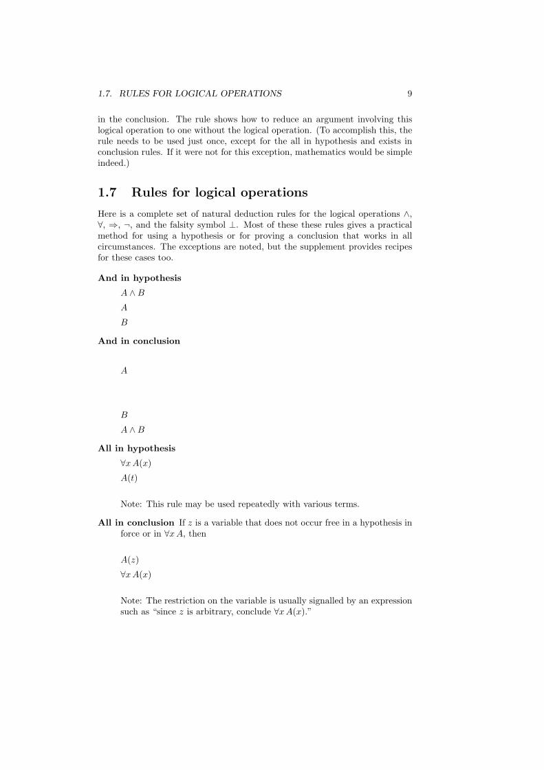
1.7 Rules for logical operations

Here is a complete set of natural deduction rules for the logical operations ∧,∀, ⇒, ¬, and the falsity symbol ⊥. Most of these these rules gives a practicalmethod for using a hypothesis or for proving a conclusion that works in allcircumstances. The exceptions are noted, but the supplement provides recipesfor these cases too.

And in hypothesis

A ∧BA

B

And in conclusion

A

B

A ∧BAll in hypothesis

∀xA(x)

A(t)

Note: This rule may be used repeatedly with various terms.

All in conclusion If z is a variable that does not occur free in a hypothesis inforce or in ∀xA, then

A(z)

∀xA(x)

Note: The restriction on the variable is usually signalled by an expressionsuch as “since z is arbitrary, conclude ∀xA(x).”


Implication in hypothesis

A⇒ B

A

B

Note: This rule by itself is an incomplete guide to practice, since it maynot be clear how to prove A. See the supplement for a variant that alwaysworks.

Implication in conclusion

Suppose A

B

Thus A⇒ B

The operation of negation ¬A is regarded as an abbreviation for A⇒ ⊥.Thus we have the following specializations of the implication rules.

Not in hypothesis

¬A

A

⊥

Note: This rule by itself is an incomplete guide to practice, since it maynot be clear how to prove A. See the supplement for a variant that alwaysworks.

Not in conclusion

Suppose A

⊥Thus ¬A

Finally, there is the famous law of contradiction.

1.8. ADDITIONAL RULES FOR OR AND EXISTS 11

Contradiction

Suppose ¬C

⊥Thus C

So far there are no rules for A∨B and for ∃xA(x). In principle one could notbother with such rules, because A∨B could always be replaced by ¬(¬A∧¬B)and ∃xA(x) could be replaced by ¬∀x¬A(x). Such a replacement is ratherclumsy and is not done in practice. Thus the following section gives additionalrules that explicitly deal with A ∨B and with ∃xA(x).

1.8 Additional rules for or and exists

Or in hypothesis

A ∨BSuppose A

C

Instead suppose B

C

Thus C

Or in conclusion

A

A ∨B

together with

B

A ∨BNote: This rule is an incomplete guide to practice. See the supplementfor a variant that always works.


Exists in hypothesis If z is a variable that does not occur free in a hypothesisin force, in ∃xA, or in C, then

∃xA(x)

Let A(z)

C

From this point on treat C as a consequence of the existential hypothesiswithout the temporary supposition A(z) or its temporary consequences.

The safe course is to take z to be a variable that is used as a temporaryname in this context, but which occurs nowhere else in the argument.

Exists in conclusion

A(t)

∃xA(x)

Note: This rule is an incomplete guide to practice. See the supplementfor a variant that always works.

1.9 Strategies for natural deduction

A natural deduction proof is read from top down. However it is often discoveredby working simultaneously from the top and the bottom, until a meeting in themiddle. The discoverer then obscures the origin of the proof by presenting itfrom the top down. This is convincing but not illuminating.Example: Here is a natural deduction proof that ∀x (x rich ⇒ x happy) leadsto ∀x (¬x happy⇒ ¬x rich).

Suppose ∀x (x rich⇒ x happy)Suppose ¬w rich

Suppose w happyw happy⇒ w richw rich⊥

Thus ¬w happyThus ¬w rich⇒ ¬w happy∀x (¬x happy⇒ ¬x rich)

There are 3 “Suppose” lines and 2 “Thus” lines. Each “Thus” removes a“Suppose.” Since 3-2 = 1, the bottom line follows from the top line alone.

Here is how to construct the proof. Start from the bottom up. To prove thegeneral conclusion, prove the implication for an arbitrary variable. To provethe implication, make a supposition. This reduces the problem to proving anegation. Then work from outside to inside. Make a supposition without the

1.9. STRATEGIES FOR NATURAL DEDUCTION 13

negation and try to get a contradiction. To accomplish this, specialize thehypothesis.Example: Here is the same proof in narrative form.

Suppose ∀x (x rich⇒ x happy). Suppose ¬w rich. Suppose w happy.Specializing the hypothesis gives w happy ⇒ w rich. So w rich. This gives afalse conclusion ⊥. Thus ¬w happy. Thus ¬w rich⇒ ¬w happy. Since w isarbitrary ∀x (6 x happy⇒ ¬x rich)Example: Here is a natural deduction proof of the fact that ∃x (x happy∧x rich)logically implies that ∃xx happy ∧ ∃xx rich.

Suppose ∃x (x happy ∧ x rich)Let z happy ∧ z richz happyz rich∃xx happy∃xx rich∃xx happy ∧ ∃xx rich

Example: Here is the same proof in narrative form.Suppose ∃x (x happy ∧ x rich). Let z happy ∧ z rich. Then z happy

and hence ∃xx happy. Similarly, z rich and hence ∃xx rich. It follows that∃xx happy ∧ ∃xx rich. Since z is an arbitrary name, this conclusion holds onthe basis of the original supposition of existence.Example: We could try to reason in the other direction, from the existence ofa happy individual and the existence of a rich individual to the existence of ahappy, rich individual? What goes wrong?

Suppose ∃xx happy∧∃xx rich. Then ∃xx happy, ∃xx rich. Let z happy.Let w rich. Then z happy ∧ w rich. This approach does not work.Example: Here is another attempt at the other direction.

Suppose ∃xx happy∧∃xx rich. Then ∃xx happy, ∃xx rich. Let z happy.Let z rich. Then z happy∧ z rich. So ∃x (x happy∧x rich). So this proves theconclusion, but we needed two temporary hypotheses on z. However we can-not conclude that we no longer need the last temporary hypothesis z rich, butonly need ∃xx rich. The problem is that we have temporarily supposed also thatz happy, and so z is not an arbitrary name for the rich individual. All this provesis that one can deduce logically from z happy, z rich that ∃x (x happy∧x rich).So this approach also does not work.Example: Here is a natural deduction proof that ∃y∀xx ≤ y gives ∀x∃y x ≤ y.

Suppose ∃y∀xx ≤ yLet ∀xx ≤ y′x′ ≤ y′∃y x′ ≤ y∀x∃y x ≤ y

Example: Here is the same proof in narrative form.Suppose ∃y∀xx ≤ y. Let y′ satisfy ∀xx ≤ y′. In particular, x′ ≤ y′.

Therefore ∃y x′ ≤ y. In fact, since y′ is just an arbitrary name, this follows onthe basis of the original existential supposition. Finally, since x′ is arbitrary,conclude that ∀x∃y x ≤ y.


A useful strategy for natural deduction is to begin with writing the hypothe-ses at the top and the conclusion at the bottom. Then work toward the middle.The most important point is to try to use the all in conclusion rule and theexists in hypothesis rule early in this process of proof construction. This intro-duces new “arbitrary” variables. Then one uses the all in hypothesis rule andthe exists in conclusion rule with terms formed from these variables. So it isreasonable to use these latter rules later in the proof construction process. Theymay need to be used repeatedly.

1.10 Lemmas and theorems

In statements of mathematical theorems it is common to have implicit universalquantifiers. For example say that we are dealing with real numbers. Instead ofstating the theorem that

∀x∀y 2xy ≤ x2 + y2 (1.7)

one simply claims that2uv ≤ u2 + v2. (1.8)

Clearly the second statement is a specialization of the first statement. But itseems to talk about u and v, and it is not clear why this might apply for someonewho wants to conclude something about p and q, such as 2pq ≤ p2 + q2. Whyis this permissible?

The answer is that the two displayed statements are logically equivalent,provided that there is no hypothesis in force that mentions the variables u orv. Then given the second statement and the fact that the variables in it arearbitrary, the first statement is a valid generalization.

Notice that there is no similar principle for existential quantifiers. The state-ment

∃xx2 = x (1.9)

is a theorem about real numbers, while the statement

u2 = u (1.10)

is a condition that is true for u = 0 or u = 1 and false for all other real numbers.It is certainly not a theorem about real numbers. It might occur in a contextwhere there is a hypothesis that u = 0 or u = 1 in force, but then it would beincorrect to generalize.

One cannot be careless about inner quantifiers, even if they are universal.Thus there is a theorem

∃xx < y. (1.11)

This could be interpreted as saying that for each arbitrary y there is a numberthat is smaller than y. Contrast this with the statement

∃x∀y x < y (1.12)

with an inner universal quantifier. This is clearly false for the real numbersystem.

1.11. RELAXED NATURAL DEDUCTION 15

1.11 Relaxed natural deduction

Mathematicians ordinarily do not care to put in all logical steps explicitly, aswould be required by the natural deduction rules. However there is a morerelaxed version of natural deduction which might be realistic in some contexts.This version omits certain trivial logical steps. Here is an outline of how it goes.

And The rules for eliminating “and” from a hypothesis and for introducing“and” in the conclusion are regarded as obvious.

All The rule for eliminating ∀xA(x) from a hypothesis by replacing it with A(t)is regarded as obvious. The rule for introducing ∀xA(x) in a conclusionis indicated more explicitly, by some such phrase as “since x is arbitrary”,which means that at this stage x does not occur as a free variable in anyhypothesis in force.

Implies The rule for eliminating ⇒ from a hypothesis is regarded as obvious.The rule for introducing ⇒ in a conclusion requires special comment. Atan earlier stage there was a Suppose A. After some logical reasoningthere is a conclusion B. Then the removal of the supposition and theintroduction of the implication is indicated by Thus A⇒ B.

Not The rule for eliminating ¬ from a hypothesis is regarded as obvious. Therule for introducing ¬ in a conclusion requires special comment. At anearlier stage there was a Suppose A. After some logical reasoning thereis a false conclusion ⊥. Then the removal of the supposition and theintroduction of the negation is indicated by Thus ¬A.

Contradiction The rule for proof by contradiction requires special comment.At an earlier stage there was a Suppose ¬A. After some logical reasoningthere is a false conclusion ⊥. Then the removal of the supposition and theintroduction of the conclusion is indicated by Thus A.

Or The rule for eliminating ∨ for the hypothesis is by proof by cases. Start withA ∨ B. Suppose A and reason to conclusion C. Instead suppose Band reason to the same conclusion C. Thus C. The rule for startingwith A (or with B) and introducing A ∨ B in the conclusion is regardedas obvious.

Exists Mathematicians tend to be somewhat casual about ∃xA(x) in a hy-pothesis. The technique is to Let A(z). Thus z is a variable that maybe used as a temporary name for the object that has been supposed toexist. (The safe course is to take a variable that will be used only in thiscontext.) Then the reasoning leads to a conclusion C that does not men-tion z. The conclusion actually holds as a consequence of the existentialhypothesis, since it did not depend on the assumption about z. The rulefor starting with A(t) and introducing ∃xA(x) is regarded as obvious.


Rules for equality (everything is equal to itself, equals may be substituted)are also used without comment.

One of the most important concepts of analysis is the concept of open set.This makes sense in the context of the real line, or in the more general case ofEuclidean space, or in the even more general setting of a metric space. Here weuse notation appropriate to the real line, but little change is required to dealwith the other cases.

For all subsets V , we say that V is open if ∀a (a ∈ V ⇒ ∃ε∀x (|x− a| < ε⇒x ∈ V )).

Recall the definition of union of a collection Γ of subsets. This says that forall y we have y ∈ ⋃Γ if and only if ∃W (W ∈ Γ ∧ y ∈W ).

Here is a proof of the theorem that for all collections of subsets Γ the hy-pothesis ∀U (U ∈ Γ ⇒ U open) implies the conclusion

⋃Γ open. The style of

the proof is a relaxed form of natural deduction in which some trivial steps areskipped.

Suppose ∀U (U ∈ Γ ⇒ U open). Suppose a ∈ ⋃Γ. By definition∃W (W ∈ Γ ∧ a ∈ W ). Let W ′ ∈ Γ ∧ a ∈ W ′. Since W ′ ∈ Γ and W ′ ∈Γ ⇒ W ′ open, it follows that W ′ open. Since a ∈ W ′ it follows from thedefinition that ∃ε∀x (|x− a| < ε ⇒ x ∈ W ′). Let ∀x (|x− a| < ε′ ⇒ x ∈ W ′).Suppose |x − a| < ε′. Then x ∈ W ′. Since W ′ ∈ Γ ∧ x ∈ W ′, it followsthat ∃W (W ∈ Γ ∧ x ∈ W ′). Then from the definition x ∈ ⋃Γ. Thus |x −a| < ε′ ⇒ x ∈ ⋃Γ. Since x is arbitrary, ∀x (|x − a| < ε′ ⇒ x ∈ ⋃Γ). So∃ε∀x (|x− a| < ε⇒ x ∈ ⋃Γ). Thus a ∈ ⋃Γ⇒ ∃ε∀x (|x− a| < ε⇒ x ∈ ⋃Γ).Since a is arbitrary, ∀a (a ∈ ⋃Γ ⇒ ∃ε∀x (|x − a| < ε ⇒ x ∈ ⋃Γ)). So bydefinition

⋃Γ open. Thus ∀U (U ∈ Γ⇒ U open)⇒ ⋃

Γ open.In practice, the natural deduction rules are useful only for the construction

of small proofs and for verification of a proof after the fact. The way to makeprogress in mathematics is find concepts that have meaningful interpretations.In order to prove a major theorem, one prepares by proving smaller theoremsor lemmas. Each of these may have a rather elementary proof. But the choiceof the statements of the lemmas is crucial in making progress. So while themicro structure of mathematical argument is based on the rules of proof, theglobal structure is a network of lemmas, theorems, and theories based on astuteselection of mathematical concepts.

To illustrate this, here is a final version of the proof that the union of acollection Γ of open subsets is open. The simplification is due to the notion ofopen ball B(a, ε), ε > 0, and the use of set notation and facts about sets. Itallows us to say that V is open if ∀a (a ∈ V ⇒ ∃εB(a, ε) ⊂ V ).

Suppose ∀U (U ∈ Γ ⇒ U open). Suppose a ∈ ⋃Γ. By definition∃W (W ∈ Γ ∧ a ∈ W ). Let W ′ ∈ Γ ∧ a ∈ W ′. Since W ′ ∈ Γ and W ′ ∈ Γ ⇒W ′ open, it follows that W ′ open. Since a ∈ W ′ it follows from the definitionthat ∃εB(a, ε) ⊂ W ′. Let B(a, ε′) ⊂ W ′. Use the fact that W ′ ∈ Γ impliesW ′ ⊂ ⋃

Γ. It follows that W ′ ⊂ ⋃Γ. Conclude that B(a, ε′) ⊂ ⋃

Γ. So∃εB(a, ε) ⊂ ⋃Γ. Thus a ∈ ⋃Γ ⇒ ∃εB(a, ε) ⊂ ⋃Γ. Since a is arbitrary,∀a (a ∈ ⋃Γ⇒ B(a, ε) ⊂ ⋃Γ). So by definition

⋃Γ open. Thus ∀U (U ∈ Γ⇒

U open)⇒ ⋃Γ open.

1.12. SUPPLEMENT: TEMPLATES 17

1.12 Supplement: Templates

Here are templates that show how to use the contradiction rule to remove theimperfections of certain of the natural deduction rules presented above. Thesetemplates are sometimes less convenient, but they always work to produce aproof, if one exists.

Implication in hypothesis template

A⇒ B

Suppose ¬C

A

B

⊥Thus C

Negation in hypothesis template

¬ASuppose ¬C

A

⊥Thus C

Note: The role of this rule to make use of a negated hypothesis ¬A. Whenthe conclusion C has no useful logical structure, but A does, then the ruleeffectively switches A for C.

Or in conclusion template Replace A ∨ B in a conclusion by ¬(¬A ∧ ¬B).Thus the template is

¬(¬A ∧ ¬B)

A ∨B.

Exists in conclusion template Replace ∃xA(x) in a conclusion by ¬(∀x¬A(x)).Thus the template is

¬(∀x¬A(x))

∃xA(x).


The Godel completeness theorem says given a set of hypotheses and a con-clusion, then either there is a proof using the natural deduction rules, or thereis an interpretation in which the hypotheses are all true and the conclusion isfalse. Furthermore, in the case when there is a proof, it may be constructed viathese templates.

Whey does this theorem not make mathematics trivial? The problem is thatif there is no proof, then the unsuccessful search for one may not terminate. Theproblem is with the rule for “all” in the hypothesis. This may be specialized inmore than one way, and there is not upper bound to the number of unsuccessfulattempts.

1.13 Supplement: Existential hypotheses

Most expositions of natural deduction give a different version of the rule for anexistential hypothesis. This rule displays the logical pattern much more clearly.Unfortunately, it is not part of everyday mathematical practice.

For the record, here is the rule:If z is a variable that does not occur free in a hypothesis in force, in ∃xA,

or in C, then

∃xA(x)Suppose A(z)

CThus C exists in hypothesis

Note: The restriction on the variable could be signalled by an expression suchas “since z is arbitrary, conclude C on the basis of the existential hypothesis∃xA(x).”

As we have seen, mathematicians tend not to use this version of the rule.They simply suppose that some convenient variable may be used as a name forthe thing that exists. They reason with this name up to a point at which theyget a conclusion that no longer mentions it. At this point they convenientlyforget the temporary supposition.Example: Here is a natural deduction proof of the fact that ∃x (x happy∧x rich)logically implies that ∃xx happy ∧ ∃xx rich.

Suppose ∃x (x happy ∧ x rich)Suppose z happy ∧ z richz happyz rich∃xx happy∃xx rich∃xx happy ∧ ∃xx rich

Thus ∃xx happy ∧ ∃xx rich

1.13. SUPPLEMENT: EXISTENTIAL HYPOTHESES 19

Example: Here is a natural deduction proof that ∃y∀xx ≤ y gives ∀x∃y x ≤ y.Suppose ∃y∀xx ≤ y

Suppose ∀xx ≤ y′x′ ≤ y′∃y x′ ≤ y

Thus ∃y x′ ≤ y∀x∃y x ≤ y

Problems

1. Quantifiers. A sequence of functions fn converges pointwise (on someset of real numbers) to f as n tends to infinity if ∀x∀ε∃N∀n(n ≥ N ⇒|fn(x) − f(x)| < ε). Here the restrictions are that x is in the set andε > 0. Show that for fn(x) = xn and for suitable f(x) there is pointwiseconvergence on the closed interval [0, 1].

2. Quantifiers. A sequence of functions fn converges uniformly (on someset of real numbers) to f as n tends to infinity if ∀ε∃N∀x∀n(n ≥ N ⇒|fn(x) − f(x)| < ε). Show that for fn(x) = xn and the same f(x) theconvergence is not uniform on [0, 1].

3. Quantifiers. Show that uniform convergence implies pointwise conver-gence.

4. Quantifiers. Show that if fn converges uniformly to f and if each fn iscontinuous, then f is continuous.

Hint: The first hypothesis is ∀ε∃N∀x∀n (n ≥ N ⇒ |fn(x) − f(x)| < ε).Deduce that ∃N∀x∀n (n ≥ N ⇒ |fn(x) − f(x)| < ε′/3). Temporarilysuppose ∀x∀n (n ≥ N ′ ⇒ |fn(x)− f(x)| < ε′/3).

The second hypothesis is ∀n∀a∀ε∃δ∀x (|x− a| < δ ⇒ |fn(x)− fn(a)| < ε).Deduce that ∃δ∀x (|x − a| < δ ⇒ |fN ′(x) − fN ′(a)| < ε′/3). Temporarilysuppose that ∀x (|x− a| < δ′ ⇒ |fN ′(x)− fN ′(a)| < ε′/3).

Suppose |x−a| < δ′. Use the temporary suppositions above to deduce that|f(x)− f(a)| < ε′. Thus |x− a| < δ′ ⇒ |f(x)− f(a)| < ε′. This is well onthe way to the desired conclusion. However be cautious: At this point x isarbitrary, but a is not arbitrary. (Why?) Explain in detail the additionalarguments to reach the goal ∀a∀ε∃δ∀x(|x− a| < δ ⇒ |f(x)− f(a)| < ε).

5. Quantifiers. A function f : R→ R is uniformly continuous iff ∀ε∃δ∀x∀y (|x−y| < δ ⇒ |f(x) − f(y)| < ε). Here ε > 0 and δ > 0 are variables re-stricted to be strictly positive. Describe the class of functions such that∀x∀y∀ε∃δ (|x− y| < δ ⇒ |f(x)− f(y)| < ε).

6. Logical deduction. Here is a mathematical argument that shows thatthere is no largest prime number. Assume that there were a largest primenumber. Call it a. Then a is prime, and for every number j with a < j,


j is not prime. However, for every number m, there is a number k thatdivides m and is prime. Hence there is a number k that divides a! + 1and is prime. Call it b. Now every number k > 1 that divides n! + 1 mustsatisfy n < k. (Otherwise it would have a remainder of 1.) Hence a < b.But then b is not prime. This is a contradiction.

Write a complete proof in outline form to show that from pure logic itfollows that the hypotheses

∀m∃k (k prime ∧ k divides m) (1.13)

∀n∀k (k divides n! + 1⇒ n < k) (1.14)

logically imply the conclusion

¬∃n (n prime ∧ ∀j (n < j ⇒ ¬ j prime)). (1.15)

7. Logical deduction. It is a well-known mathematical fact that√

2 is ir-rational. In fact, if it were rational, so that

√2 = m/n, then we would

have 2n2 = m2. Thus m2 would have an even number of factors of 2,while 2n2 would have an odd number of factors of two. This would be acontradiction.

Show that from logic alone it follows that

∀i i2 even-twos (1.16)

and∀j (j even-twos⇒ ¬(2 · j) even-twos) (1.17)

give¬∃m∃n (2 · n2) = m2. (1.18)

8. Logical deduction. If X is a set, then P (X) is the set of all subsets ofX. If X is finite with n elements, then P (X) is finite with 2n elements.A famous theorem of Cantor states that there is no function f from Xto P (X) that is onto P (X). Thus in some sense there are more elementsin P (X) than in X. This is obvious when X is finite, but the interestingcase is when X is infinite.

Here is an outline of a proof. Consider an arbitrary function f from Xto P (X). We want to show that there exists a set V such that for eachx in X we have f(x) 6= V . Consider the condition that x /∈ f(x). Thiscondition defines a set. That is, there exists a set U such that for all x,x ∈ U is equivalent to x /∈ f(x). Call this set S. Let p be arbitrary.Suppose f(p) = S. Suppose p ∈ S. Then p /∈ f(p), that is, p /∈ S. Thisis a contradiction. Thus p /∈ S. Then p ∈ f(p), that is, p ∈ S. This is acontradiction. Thus f(p) 6= S. Since this is true for arbitrary p, it followsthat for each x in X we have f(x) 6= S. Thus there is a set that is not inthe range of f .

1.13. SUPPLEMENT: EXISTENTIAL HYPOTHESES 21

Show that from logic alone it follows that from

∃U ∀x ((x ∈ U ⇒ ¬x ∈ f(x)) ∧ (¬x ∈ f(x)⇒ x ∈ U)) (1.19)

one can conclude that∃V ∀x¬f(x) = V. (1.20)

9. Logical deduction. Here is an argument that if f and g are continuousfunctions, then the composite function gf defined by (gf)(x) = g(f(x))is a continuous function.Assume that f and g are continuous. Consider an arbitrary point a′

and an arbitrary ε′ > 0. Since g is continuous at f(a′), there existsa δ > 0 such that for all y the condition |y − f(a′)| < δ implies that|g(y)− g(f(a′))| < ε′. Call it δ1. Since f is continuous at a′, there exists aδ > 0 such that for all x the condition |x−a′| < δ implies |f(x)− f(a′)| <δ1. Call it δ2. Consider an arbitrary x′. Suppose |x′ − a′| < δ2. Then|f(x′)− f(a′)| < δ1. Hence |g(f(x′))− g(f(a′))| < ε′. Thus |x′ − a′| < δ2implies |g(f(x′))− g(f(a′))| < ε′. Since x′ is arbitrary, this shows that forall x we have the implication |x−a′| < δ2 implies |g(f(x))−g(f(a′))| < ε′.It follows that there exists δ > 0 such that all x we have the implication|x − a′| < δ implies |g(f(x)) − g(f(a′))| < ε′. Since ε′ is arbitrary, thecomposite function g f is continuous at a′. Since a′ is arbitrary, thecomposite function g f is continuous.In the following proof the restrictions that ε > 0 and δ > 0 are implicit.They are understood because this is a convention associated with the useof the variables ε and δ.Prove that from

∀a∀ε∃δ∀x (|x− a| < δ ⇒ |f(x)− f(a)| < ε) (1.21)

and∀b∀ε∃δ∀y (|y − b| < δ ⇒ |g(y)− g(b)| < ε) (1.22)

one can conclude that

∀a∀ε∃δ∀x (|x− a| < δ ⇒ |g(f(x))− g(f(a))| < ε). (1.23)

10. Relaxed natural deduction. Take the proof that the union of open sets isopen and put it in outline form, with one formula per line. Indent at everySuppose line. Remove the indentation at every Thus line. (However,do not indent at a Let line.)

11. Draw a picture to illustrate the proof in the preceding problem.

12. Relaxed natural deduction. Prove that for all subsets U, V that (U open∧V open) ⇒ U ∩ V open. Recall that U ∩ V =

⋂U, V is defined byrequiring that for all y that y ∈ U ∩ V ⇔ (y ∈ U ∧ y ∈ V ). It may behelpful to use the general fact that for all t, ε1 > 0, ε2 > 0 there is animplication t < min(ε1, ε2) ⇒ (t < ε1 ∧ t < ε2). Use a relaxed naturaldeduction format. Put in outline form, with one formula per line.


13. Draw a picture to illustrate the proof in the preceding problem.

14. Relaxed natural deduction. Recall that for all functions f , sets W , andelements t we have t ∈ f−1[W ] ⇔ f(t) ∈ W . Prove that f continuous(with the usual ε-δ definition) implies ∀U (U open⇒ f−1[U ] open).

15. Relaxed natural deduction. It is not hard to prove the lemma y | |y−b| <ε open. Use this lemma and the appropriate definitions to prove that∀U (U open⇒ f−1[U ] open) implies f continuous.

Chapter 2

Sets

2.1 Zermelo axioms

Mathematical objects include sets, functions, and numbers. It is natural tobegin with sets. If A is a set, the expression

t ∈ A (2.1)

can be read simply “t in A”. Alternatives are “t is a member of A, or “t is anelement of A”, or “t belongs to A”, or “t is in A”. The expression ¬t ∈ A isoften abbreviated t /∈ A and read “t not in A”.

If A and B are sets, the expression

A ⊂ B (2.2)

is defined in terms of membership by

∀t (t ∈ A⇒ t ∈ B). (2.3)

This can be read simply “A subset B.” Alternatives are “A is included in B”or “A is a subset of B”. (Some people write A ⊆ B to emphasize that A = Bis allowed, but this is a less common convention.) It may be safer to avoid suchphrases as “t is contained in A” or “A is contained in B”, since here practice isambiguous. Perhaps the latter is more common.

The following axioms are the starting point for Zermelo set theory. Theywill be supplemented later with the axiom of infinity and the axiom of choice.These axioms are taken by some to be the foundations of mathematics; howeverthey also serve as a review of important constructions.

Extensionality A set is defined by its members. For all sets A,B

(A ⊂ B ∧B ⊂ A)⇒ A = B. (2.4)

23

24 CHAPTER 2. SETS

Empty set Nothing belongs to the empty set.

∀y y /∈ ∅. (2.5)

Unordered pair For all objects a, b the unordered pair set a, b satisfies

∀y (y ∈ a, b ⇔ (y = a ∨ y = b)). (2.6)

Union If Γ is a set of sets, then its union⋃

Γ satisfies

∀x (x ∈⋃

Γ⇔ ∃A (A ∈ Γ ∧ x ∈ A)) (2.7)

Power set If X is a set, the power set P (X) is the set of all subsets of X, so

∀A (A ∈ P (X)⇔ A ⊂ X). (2.8)

Selection Consider an arbitrary condition p(x) expressed in the language ofset theory. If B is a set, then the subset of B consisting of elements thatsatisfy that condition is a set x ∈ B | p(x) satisfying

∀y (y ∈ x ∈ B | p(x) ⇔ (y ∈ B ∧ p(y))). (2.9)

2.2 Comments on the axioms

Usually in a logical language there is the logical relation symbol = and a numberof additional relation symbols and function symbols. The Zermelo axioms couldbe stated in an austere language in which the only non-logical relation symbolis ∈, and there are no function symbols. The only terms are variables. Whilethis is not at all convenient, it helps to give a more precise formulation of theselection axiom. The following list repeats the axioms in this limited language.However, in practice the other more convenient expressions for forming termsare used.

The philosophy of Zermelo set theory is that everything is a set. Howeverit is helpful at times to think of a hierarchy of objects of different types. Anobject whose internal structure is of no interest is a point. A set is defined byits members, which may be points. A collection is a set whose members arethemselves sets. Sometimes a collection is called a family.

Extensionality∀A∀B (∀t (t ∈ A⇔ t ∈ B)⇒ A = B). (2.10)

The axiom of extensionality says that a set is defined by its members.Thus, if A is the set consisting of the digits that occur at least once inmy car’s license plate 5373, and if B is the set consisting of the odd onedigit prime numbers, then A = B is the same three element set. All thatmatters are that its members are the numbers 7,3,5.

2.2. COMMENTS ON THE AXIOMS 25

Empty set∃N∀y ¬y ∈ N. (2.11)

By the axiom of extensionality there is only one empty set, and in practiceit is denoted by the conventional name ∅.

Unordered pair∀a∀b∃E∀y (y ∈ E ⇔ (y = a ∨ y = b)). (2.12)

By the axiom of extensionality, for each a, b there is only one unorderedpair a, b. The unordered pair construction has this name because theorder does not matter: a, b = b, a. Notice that this set can have eitherone or two elements, depending on whether a = b or a 6= b. In the casewhen it has only one element, it is written a and is called a singletonset.

If a, b, c are objects, then there is a set a, b, c defined by the conditionthat for all y

y ∈ a, b, c ⇔ (y = a ∨ y = b ∨ y = c). (2.13)

This is the corresponding unordered triple construction. The existence ofthis object is easily seen by noting that both a, b and b, c exist by theunordered pair construction. Again by the unordered pair constructionthe set a, b, b, c exists. But then by the union construction the set⋃a, b, b, c exists. A similar construction works for any finite numberof objects.

Union∀Γ∃U∀x (x ∈ U ⇔ ∃A (A ∈ Γ ∧ x ∈ A)) (2.14)

The standard name for the union is⋃

Γ. Notice that⋃ ∅ = ∅ and⋃

P (X) = X. A special case of the union construction is A ∪ B =⋃A,B. This satisfies the property that for all x

x ∈ A ∪B ⇔ (x ∈ A ∨ x ∈ B). (2.15)

Suppose that C ⊂ X is a given subset of X and that Γ is a collection ofsubsets of X. Then Γ is said to be a cover of C provided C ⊂ ⋃Γ.

If Γ 6= ∅ is a set of sets, then the intersection⋂

Γ is defined by requiringthat for all x

x ∈⋂

Γ⇔ ∀A (A ∈ Γ⇒ x ∈ A) (2.16)

The existence of this intersection follows from the union axiom and theselection axiom:

⋂Γ = x ∈ ⋃Γ | ∀A (A ∈ Γ⇒ x ∈ A).

There is a peculiarity in the definition of⋂

Γ when Γ = ∅. If there is acontext where X is a set and Γ ⊂ P (X), then we can define

⋂Γ = x ∈ X | ∀A (A ∈ Γ⇒ x ∈ A). (2.17)

26 CHAPTER 2. SETS

If Γ 6= ∅, then this definition is independent of X and is equivalent tothe previous definition. On the other hand, by this definition

⋂ ∅ = X.This might seem strange, since the left hand side does not depend on X.However in most contexts there is a natural choice of X, and this is thedefinition that is appropriate to such contexts. There is a nice symmetrywith the case of union, since for the intersection

⋂ ∅ = X and⋂P (X) = ∅.

A special case of the intersection construction is A ∩B =⋂A,B. This

satisfies the property that for all x

x ∈ A ∩B ⇔ (x ∈ A ∧A ∈ B). (2.18)

If A ⊂ X, the relative complement X \ A is characterized by saying thatfor all x

x ∈ X \A⇔ (x ∈ X ∧ x /∈ A). (2.19)

The existence again follows from the selection axiom: X \ A = x ∈ X |x /∈ A. Sometimes when the set X is understood the complement X \Aof A is denoted Ac.

The constructions A∩B, A∪B,⋂

Γ,⋃

Γ, and X \A are means of produc-ing objects that have a special relationship to the corresponding logicaloperations ∧,∨,∀,∃,¬. A look at the definitions makes this apparent.

Two sets A,B are disjoint if A ∩ B = ∅. (In that case it is customary towrite the union of A and B as AtB.) More generally, a set Γ ⊂ P (X) ofsets is disjoint if for each A in Γ and B ∈ Γ with A 6= B we have A∩B = ∅.A partition of X is a set Γ ⊂ P (X) such that Γ is disjoint and ∅ /∈ Γ and⋃

Γ = X.

Power set∀X∃P∀A (A ∈ P ⇔ ∀t (t ∈ A⇒ t ∈ X)). (2.20)

The power set is the set of all subsets of X, and it is denoted P (X).Since a large set has a huge number of subsets, this axiom has strongconsequences for the size of the mathematical universe.

Selection The selection axiom is really an infinite family of axioms, one foreach formula p(x) expressed in the language of set theory.

∀B∃S∀y (y ∈ S ⇔ (y ∈ B ∧ p(y))). (2.21)

The selection axiom says that if there is a set B, then one may select asubset x ∈ B | p(x) defined by a condition expressed in the languageof set theory. The language of set theory is the language where the onlynon-logical relation symbol is ∈. This is why it is important to realize thatin principle the other axioms may be expressed in this limited language.The nice feature is that one can characterize the language as the one withjust one non-logical relation symbol. However the fact that the separationaxiom is stated in this linguistic way is troubling for one who believes thatwe are talking about a Platonic universe of sets.

2.3. ORDERED PAIRS AND CARTESIAN PRODUCT 27

Of course in practice one uses other ways of producing terms in the lan-guage, and this causes no particular difficulty. Often when the set B isunderstood the set is denoted more simply as x | p(x). In the definingcondition the quantified variable is implicitly restricted to range over B, sothat the defining condition is that for all y we have y ∈ x | p(x) ⇔ p(y).The variables in the set builder construction are bound variables, so, forinstance, u | p(u) is the same set as t | p(t).The famous paradox of Bertrand Russell consisted of the discovery thatthere is no sensible way to define sets by conditions in a completely unre-stricted way. The idea is to note that y ∈ x is defined for every orderedpair of sets x, y. Consider the diagonal where y = x. Either x ∈ x orx /∈ x. If there were a set a = x | x /∈ x, then a ∈ a would be equivalentto a /∈ a, which is a contradiction.

Say that it is known that for every x in A there is another correspondingobject φ(x) in B. Then another useful notation is

φ(x) ∈ B | x ∈ A ∧ p(x). (2.22)

This can be defined to be the set

y ∈ B | ∃x (x ∈ A ∧ p(x) ∧ y = φ(x). (2.23)

So it is a special case. Again, this is often abbreviated as φ(x) | p(x)when the restrictions on x and φ(x) are clear. In this abbreviated notionone could also write the definition as y | ∃x (p(x) ∧ y = φ(x)).

2.3 Ordered pairs and Cartesian product

There is also a very important ordered pair construction. If a, b are objects,then there is an object (a, b). This ordered pair has the following fundamentalproperty: For all a, b, p, q we have

(a, b) = (p, q)⇔ (a = p ∧ b = q). (2.24)

If y = (a, b) is an ordered pair, then the first coordinates of y is a and the secondcoordinate of y is b.

Some mathematicians like to think of the ordered pair (a, b) as the set (a, b) =a, a, b. The purpose of this rather artificial construction is to make it amathematical object that is a set, so that one only needs axioms for sets, andnot for other kinds of mathematical objects. However this definition does notplay much of a role in mathematical practice.

There are also ordered triples and so on. The ordered triple (a, b, c) is equalto the ordered triple (p, q, r) precisely when a = p and b = q and c = r. Ifz = (a, b, c) is an ordered triple, then the coordinates of z are a, b and c. Onecan construct the ordered triple from ordered pairs by (a, b, c) = ((a, b), c). Theordered n-tuple construction has similar properties.

28 CHAPTER 2. SETS

There are degenerate cases. There is an ordered 1-tuple (a). If x = (a), thenits only coordinate is a. Furthermore, there is an ordered 0-tuple ( ) = 0 = ∅.

Corresponding to these constructions there is a set construction called Carte-sian product. If A,B are sets, then A × B is the set of all ordered pairs (a, b)with a ∈ A and b ∈ B. This is a set for the following reason. Let U = A ∪ B.Then each of a and a, b belongs to P (U). Therefore the ordered pair (a, b)belongs to P (P (U)). This is a set, by the power set axiom. So by the selectionaxiom A×B = (a, b) ∈ P (P (U)) | a ∈ A ∧ b ∈ B is a set.

One can also construct Cartesian products with more factors. Thus A×B×Cconsists of all ordered triples (a, b, c) with a ∈ A and b ∈ B and c ∈ C.

The Cartesian product with only one factor is the set whose elements arethe (a) with a ∈ A. There is a natural correspondence between this somewhattrivial product and the set A itself. The correspondence is that which associatesto each (a) the corresponding coordinate a. The Cartesian product with zerofactors is a set 1 = 0 with precisely one element 0 = ∅.

There is a notion of sum of sets that is dual to the notion of product ofsets. This is the disjoint union of two sets. The idea is to attach labels to theelements of A and B. Thus, for example, for each element a of A consider theordered pair (0, a), while for each element b of B consider the ordered pair (1, b).Then even if there are elements common to A and B, their tagged versions willbe distinct. Thus the sets 0×A and 1×B are disjoint. The disjoint unionof A and B is the set A+B such that for all y

y ∈ A+B ⇔ (y ∈ 0 ×A ∨ y ∈ 1 ×B). (2.25)

One can also construct disjoint unions with more summands in the obvious way.

2.4 Relations and functions

A relation R between sets A and B is a subset of A×B. A function F from Ato B is a relation with the following two properties:

∀x∃y (x, y) ∈ F. (2.26)

∀y∀y′ (∃x ((x, y) ∈ F ∧ (x, y′) ∈ F )⇒ y = y′). (2.27)

In these statements the variable x is restricted to A and the variables y, y′ arerestricted to B. A function F from A to B is a surjection if

∀y∃x (x, y) ∈ F. (2.28)

A function F from A to B is an injection if

∀x∀x′ (∃y ((x, y) ∈ F ∧ (x′, y) ∈ F )⇒ x = x′). (2.29)

Notice the same pattern in these definitions as in the two conditions that definea function. As usual, if F is a function, and (x, y) ∈ F , then we write F (x) = y.

2.5. NUMBER SYSTEMS 29

In this view a function is regarded as being identical with its graph as asubset of the Cartesian product. On the other hand, there is something to besaid for a point of view that makes the notion of a function just as fundamentalas the notion of set. In that perspective, each function from A to B would havea graph that would be a subset of A× B. But the function would be regardedas an operation with an input and output, and the graph would be a set thatis merely one means to describe the function.

There is a useful function builder notation that corresponds to the set buildernotation. Say that it is known that for every x in A there is another correspond-ing object φ(x) in B. Then another useful notation is

x 7→ φ(x) : A→ B = (x, φ(x)) ∈ A×B | x ∈ A. (2.30)

This is an explicit definition of a function from A to B. This could be ab-breviated as x 7→ φ(x) when the restrictions on x and φ(x) are clear. Thevariables in such an expression are of course bound variables, so, for instance,the squaring function u 7→ u2 is the same as the squaring function t 7→ t2.

2.5 Number systems

The axiom of infinity states that there is an infinite set. In fact, it is handy tohave a specific infinite set, the set of all natural numbers N = 0, 1, 2, 3, . . ..The mathematician von Neumann gave a construction of the natural numbersthat is perhaps too clever to be taken entirely seriously. He defined 0 = ∅,1 = 0, 2 = 0, 1, 3 = 0, 1, 2, and so on. Each natural number is the setof all its predecessors. Furthermore, the operation s of adding one has a simpledefinition:

s(n) = n ∪ n. (2.31)

Thus 4 = 3 ∪ 3 = 0, 1, 2 ∪ 3 = 0, 1, 2, 3. Notice that each of these setsrepresenting a natural number is a finite set. There is as yet no requirementthat the natural numbers may be combined into a single set.

This construction gives one way of formulating the axiom of infinity. Saythat a set I is inductive if 0 ∈ I and ∀n (n ∈ I ⇒ s(n) ∈ I). The axiomof infinity says that there exists an inductive set. Then the set N of naturalnumbers may be defined as the intersection of the inductive subsets of this set.

According to this definition the natural number system N0, 1, 2, 3, . . . has0 as an element. It is reasonable to consider 0 as a natural number, since it is apossible result of a counting process. However it is sometimes useful to considerthe set of natural numbers with zero removed. In this following we denote thisset by by N+ = 1, 2, 3, . . ..

According to the von Neuman construction, the natural number n is definedby n = 0, 1, 2, . . . , n−1. This is a convenient way produce an n element indexset, but in other contexts it can also be convenient to use 1, 2, 3, . . . , n.

This von Neumann construction is only one way of thinking of the set ofnatural numbers N. However, once we have this infinite set, it is not difficult

30 CHAPTER 2. SETS

to construct a set Z consisting of all integers . . . ,−3,−2,−1, 0, 1, 2, 3, . . ..Furthermore, there is a set Q of rational numbers, consisting of all quotientsof integers, where the denominator is not allowed to be zero. The next stepafter this is to construct the set R of real numbers. This is done by a process ofcompletion, to be described later. The transition from Q to R is the transitionfrom algebra to analysis. The result is that it is possible to solve equations byapproximation rather than by algebraic means.

After that, next important number system is C, the set of complex numbers.Each complex number is of the form a + bi, where a, b are real numbers, andi2 = −1. Finally, there is H, the set of quaternions. Each quaternion is ofthe form t + ai + bj + ck, where t, a, b, c are real numbers. Here i2 = −1, j2 =−1, k2 = −1, ij = k, jk = i, ki = j, ji = −k, kj = −i, ik = −j. A purequaternion is one of the form ai+ bj+ ck. The product of two pure quaternionsis (ai+ bj+ ck)(a′i+ b′j+ c′k) = −(aa′+ bb′+ cc′) + (bc′− cb′)i+ (ca′− ac′)j+(ab′− ba′)k. Thus quaternion multiplication includes both the dot product andthe cross product in a single operation.

In summary, the number systems of mathematics are N,Z,Q,R,C,H. Thesystems N,Z,Q,R each have a natural linear order, and there are natural orderpreserving injective functions from N to Z, from Z to Q, and from Q to R. Thenatural algebraic operations in N are addition and multiplication. In Z theyare addition, subtraction, and multiplication. In Q,R,C,H they are addition,subtraction, multiplication, and division by non-zero numbers. In H the multi-plication and division are non-commutative. The number systems R,C,H havethe completeness property, and so they are particularly useful for analysis.

2.6 The extended real number system

In analysis it is sometimes useful to have an extended real number system,consisting of R together with two extra points +∞ and−∞. The order structureis that −∞ ≤ a ≤ +∞ for all real numbers a. The purpose of this system isnot to clarify the notion of infinity; rather it is to have an extended real numbersystem with a greatest element and a least element. It is possible to talk aboutcontinuity in the extended real number system, for instance by mapping it to[−1, 1] via the hyperbolic tangent function.

The arithmetic in [−∞,+∞] is worth some discussion. If a > 0 is an ex-tended real number, it is natural to define a · (±∞) = ±∞. Similarly, if a < 0is an extended real number, it is natural to define a · (±∞) = ∓∞. For zerothere is a zero times infinity convention that is often used in analysis:

0 · (±∞) = 0. (2.32)

The difficult with this convention is that it makes multiplication discontinuous.To see, this, note that while (1/n) ·n = 1→ 1 as n→∞, the limit of 1/n timesthe limit of n is 0 · (+∞) = 0.

Addition is even worse. While a + (+∞) = +∞ for all a > −∞, and a +(−∞) = −∞ for all a < +∞, the expressions (−∞) + (+∞) and (+∞) + (−∞)

2.7. SUPPLEMENT: CONSTRUCTION OF NUMBER SYSTEMS 31

are undefined. This infinity minus infinity problem is the source of many of themost interesting phenomena of analysis. On the other hand, where addition isdefined, it is continuous.

For some purposes one can get around the infinity minus infinity problemby using the systems (−∞,+∞] or by using the system [−∞,+∞). For eitherof these systems both addition and multiplication are defined.

2.7 Supplement: Construction of number sys-tems

This section gives an outline of the construction of various number systems. Thepurpose of these constructions is merely to show that the existence of numbersystems follows from the assumptions of set theory. There is no claim that theyexplain what numbers really are.

It is assumed that there is a natural number system N with a zero 0 and asuccessor operation s such that s(n) is the next integer above n. (In the vonNeumann construction 0 is the empty set and s(n) = n∪n.) The characteristicfeature is the induction property: If J is inductive, then N ⊂ J .

Addition in N may then be characterized inductively by m + 0 = 0 andm+s(n) = s(m+n). Similarly, multiplication may be characterized by m ·0 = 0and m · s(n) = m · n+m. It is a tedious process to verify the properties of theoperations by induction, but it can be done.

Next is the construction of the integers Z. Consider the product space N×N.The intuitive idea is that each point (m,n) in this space is to define an integerk with k = n −m. This idea leads to the following definitions. If the orderedpairs (m,n) and (m′, n′) are in this space, then their sum is the vector sum(m,n) + (m′, n′) = (m + m′, n + n′). The additive inverse of (m,n) is defined(somewhat unusually) as −(m,n) = (n,m). The product of (m,n) and (m′, n′)has components given by inner products ((m,n) · (m′, n′), (n,m) · (m′, n′)). Thisworks out to be (mm′ + nn′, nm′ + mn′). Two such ordered pairs (m,n) and(m′, n′) are said to be equivalent if m+n′ = n+m′. This relation of equivalencepartitions N × N into a disjoint union of sets. Each such set of ordered pairsdefines an integer.

If we consider N × N geometrically, then each integer is the graph of a linewith slope one. The sum of two integers is determined by taking the vector sumof any two points on the two lines. The inverse is obtained by reflecting pointsacross the diagonal line passing through the origin. The product is obtained bytaking a point to another point with coordinates given by the product formulaabove, which only involves inner products and the reflection across the diagonal.

Thus, for example, the integer 3 is defined as the right shift 3 = (0, 3), (1, 4), (2, 5), . . .on the natural numbers. The integer −5 is defined as the left shift −5 =(5, 0), (6, 1), (7, 2), . . .. To add the integer 3 to the integer -5, take a rep-resentative (1, 4) and another representative (7, 2). Add to get (8, 6), whichrepresents −2.

32 CHAPTER 2. SETS

Next is the construction of the rational numbers Q. Start with the integersZ. Let Z∗ be Z with the integer zero removed. Consider the product spaceZ∗ × Z. The intuitive idea is that each point (j, k) with j 6= 0 in this space isto define a rational number q with q = k/j. This idea leads to the followingdefinitions. If the ordered pairs (j, k) and (j′, k′) are in this space, then theirproduct is the pointwise product (j · j′, k · k′). (Multiply the denominators;multiply the numerators.) The multiplicative inverse of (j, k) for j, k 6= 0 isdefined as the reflection (k, j). (Interchange numerator and denominator.) Twosuch ordered pairs (j, k) and (j′, k′) are said to be equivalent if j · k′ = k · j′.This relation of equivalence partitions Z∗×Z into a disjoint union of sets. Eachsuch set of ordered pairs defines a rational number.

If we consider Z∗ × Z geometrically, then each rational is the graph of aline through the origin. Thus, for example, the rational number 4/3 is definedas 4/3 = (3, 4), (−3,−4), (6, 8), (−6,−8), . . .. The rational number −5/2 isdefined as −5/2 = (2,−5), (−2, 5), (4,−10), (−4, 10), . . .. To multiply integer4/3 by −5/2 , take a representative (3, 4) and another representative (4,−10).Use the multiplication rule to get (12,−40), which represents −10/3. Thisdiscussion has left out addition of rational numbers; this dismal story is all toowell known.

The construction of the rational numbers from the integers is quite parallelto the construction of the integers from the natural numbers. The constructionof the real numbers is quite another matter. This construction is explored indetail in the chapter on ordered sets. However here is the short version.

Most real numbers are not rational, but it is tricky to prove that individualreal numbers are not rational. Here is an example of a real number that isnot rational. Let sn = 1 + 1 + 1/2 + 1/6 + · · · 1/n!. This is clearly a rationalnumber, and the real number e is the real number that is the supremum orleast upper bound of the sn. The property that makes e irrational is that itcan be approximated very closely by a rational number that is not equal to it.Specifically, by Taylor’s theorem with remainder,

e = 1 + 1 +12

+16

+ · · · 1n!

+ecn

(n+ 1)!, (2.33)

where 0 < cn < 1 and hence 1 < ecn < 3. This shows that e is a rationalnumber (the partial sum) plus a very small number (the remainder). Supposethat e were rational, e = p/q, with integer p, q > 0. Then

n!p = qn![1 + 1 +

12

+16

+ · · · 1n!

]+ q

ecn

n+ 1, (2.34)

The numbers p and q are fixed. Choose n large enough so that n+1 > 3q. Then0 < qecn/(n+ 1) < 1. However all the other terms are integers. This leads to acontradiction. So e is not rational.

The problem is to construct the real numbers R from the rational numbers.This is the crucial step in the passage from algebra to analysis. In the construc-tion each real number will be a set of rational numbers, but only certain sets

2.7. SUPPLEMENT: CONSTRUCTION OF NUMBER SYSTEMS 33

are used. That is, the each real number will belong to the (huge) set P (Q), butnot all sets will be used.

If A is a set of rational numbers, an upper bound for A is a rational numberq such that each x in A satisfies x ≤ A. Let ↑ A be the set of all upper boundsfor A. If B is a set of rational numbers, a lower bound for B is a rational numberp such that each x in B satisfies x ≤ p. Let ↓ B be the set of all lower boundsfor B. Clearly A ⊂↓↑ A. Call a set A of rational numbers a lower Dedekindcut if ↓↑ A ⊂ A. Then R is defined as the set of all lower Dedekind cuts A suchthat A 6= ∅ and ↑ A 6= ∅.

If r is a rational number, then the set of lower bounds for r is a lowerDedekind cut. So each rational number defines a real number. For instance, therational number 4/3 defines the real number consisting of all rational numbersp with p ≤ 4/3. However there are real numbers that are not rational numbers.For instance, let S be the set of all rational numbers of the form sn = 1 + 1 +1/2 + 1/6 + · · · 1/n!. Let A =↓↑ S. Then A is a real number that does not comefrom a rational number. The intuition is that ↑ S consists of the rational upperbounds for e, and A =↓↑ S consists of the rational lower bounds for e.

If A and A′ are real numbers, regarded as lower Dedekind cuts, then A ≤ A′means A ⊂ A′. This defines the order structure on real numbers. Defining theadditive structure is easy; the sum A+ A′ of two lower Dedekind cuts consistsof the set of all rational sums x + x′ with x in A and x′ in A′. Defining themultiplicative structure is more awkward, but it can be done.

The real number system R has the property that it is boundedly complete.That is, every non-empty subset of R that is bounded above has a supremum(least upper bound). It is not hard to see this from the construction. Each realnumber in the subset is itself a lower Dedekind cut. The union of these may ormay not be a lower Dedekind cut, but there is a smallest lower Dedekind cut ofwhich the union is a subset. This is the supremum.

Problems

1. Say X has n elements. How many elements are there in P (X)?

2. Say X has n elements. Denote the number of subsets of X with exactlyk elements by

(nk

). Show that

(n0

)= 1 and

(nn

)= 1 and that

(n

k

)=(n− 1k − 1

)+(n− 1k

). (2.35)

Use this to make a table of(nk

)up to n = 7.

3. Say that X has n elements. Denote the number of partitions of X intoexactly k non-empty disjoint subsets by S(n, k). This is a Stirling numberof the second kind. Show that S(n, 1) = 1 and S(n, n) = 1 and

S(n, k) = S(n− 1, k − 1) + kS(n− 1, k). (2.36)

Use this to make a table of S(n, k) up to n = 5.

34 CHAPTER 2. SETS

4. How many functions are there from an n element set to a k element set?

5. How many injective functions are there from an n element set to a kelement set?

6. How many surjective functions are there from an n element set to a kelement set?

7. Show that mn =∑mk=0

(mk

)k!S(n, k).

8. Let Bn =∑nk=0 S(n, k) be the number of partitions of an n element

set. Show that Bn is equal to the expected number of functions from ann element set to an m element set, where m has a Poisson probabilitydistribution with mean one. That is, show that

Bn =∞∑m=0

mn 1m!e−1. (2.37)

9. Let Bn be the number of partitions of an n element set into disjoint non-empty sets. Thus B0 = 1, B1 = 1, B2 = 2, B3 = 5, B4 = 15, B5 = 52, andso on. One can try to write Bn+1 as a linear combination of B0, . . . , Bn.For instance,

B3 = B2 + 2B1 +B0 (2.38)

andB4 = B3 + 3B2 + 3B1 +B0 (2.39)

andB5 = B4 + 4B3 + 6B2 + 4B1 +B0. (2.40)

Find the general pattern. Prove that it holds for arbitrary n. Hint: Con-sider a set S with n+ 1 points, with a selected point p in it.

10. Is it possible to have sets A and B, a function f : A → B that is aninjection but not a surjection, and a function g : A→ B that is a surjectionbut not an injection. Explain.

11. A totally ordered set is densely ordered if between every two distinct pointsthere is another point. Thus Q is densely ordered, and also R is denselyordered. Show that between every two distinct points of Q there is a pointof R that is irrational.

12. Is it true that between every two distinct points of R there is a point ofQ? Discuss.

13. Define a map from R to P (Q) by j(x) = r ∈ Q | r ≤ x. Prove that j isinjective.

Chapter 3

Relations, functions,dynamical systems

3.1 Identity, composition, inverse, intersection

A relation R between sets A and B is a subset of A × B. In this context oneoften writes xRy instead of (x, y) ∈ R, and says that x is related to y by therelation. Often a relation between A and A is called a relation on the set A.

There is an important relation IA on A, namely the identity relation relationconsisting of all ordered pairs (x, x) with x ∈ A. That is, for x and y in A, therelation xIAy is equivalent to x = y.

Given an relation R between A and B and a relation S between B and C,there is a relation S R between A and C called the composition. It is definedin such a way that x(S R)z is equivalent to the existence of some y in B suchthat xRy and ySz. Thus if R relates A to B, and S relates B to C, then S Rrelates A to C. In symbols,

S R = (x, z) | ∃y (xRy ∧ ySz). (3.1)

Notice the order in which the factors occur, which accords with the usual con-vention for functions. For functions it is usual to use such a notation to indicatethat R acts first, and then S. This is perhaps not the most natural conventionfor relations, so in some circumstances it might be convenient to define anotherkind of composition in which the factors are written in the opposite order.

There are two more useful operations on relations. If R is a relation betweenA and B, then there is an inverse relation R−1 between B and A. It consistsof all the (y, x) such that (x, y) is in R. That is, yR−1x is equivalent to xRy.

Finally, if R and S are relations between A and B, then there is a relationR ∩ S. This is also a useful operation. Notice that R ⊂ S is equivalent toR ∩ S = R.

Sometimes if X ⊂ A one writes R[X] for the image of X under R, that is,

R[X] = y | ∃x (x ∈ X ∧ xRy). (3.2)

35

36 CHAPTER 3. RELATIONS, FUNCTIONS, DYNAMICAL SYSTEMS

Also, if a is in A, it is common to write R[a] instead of R[a]. Thus y is inR[a] if aRy.

3.2 Picturing relations

There are two common ways of picturing a relation R between A and B. Oneway is to draw the product space A×B and sketch the set of points (x, y) in R.This is the graph of the relation. The other way is to draw the disjoint unionA+B and for each (x, y) in R sketch an arrow from x to y. This is the cographof the relation.

3.3 Equivalence relations

Consider a relation R on A. The relation R is reflexive if IA ⊂ R. The relationR is symmetric if R = R−1. The relation R is transitive if R R ⊂ R. A rela-tion that is reflexive, symmetric, and transitive (RST) is called an equivalencerelation.

Theorem 3.1 Consider a set A. Let Γ be a partition of A. Then there is acorresponding equivalence relation E, such that (x, y) ∈ E if and only if forsome subset U in Γ both x in U and y in U . Conversely, for every equivalencerelation E on A there is a unique partition Γ of A that gives rise to the relationin this way.

The sets in the partition defined by the equivalence relation are called theequivalence classes of the relation.

3.4 Generating relations

Theorem 3.2 For every relation R on A, there is a smallest transitive relationRT such that R ⊂ RT . This is the transitive relation generated by R.

Theorem 3.3 For every relation R on A, there is a smallest symmetric andtransitive relation RST such that R ⊂ RST . This is the symmetric and transitiverelation generated by R.

Theorem 3.4 For every relation R on A, there is a smallest equivalence rela-tion E = RRST such that R ⊂ E. This is the equivalence relation generated byR.

Proof: The proofs of these theorems all follow the same pattern. Here isthe proof of the last one. Let R be a relation on A, that is, let R be a subset ofA×A. Let ∆ be the set of all equivalence relations S with R ⊂ S. Then sinceA×A ∈ ∆, it follows that ∆ is non-empty. Let E =

⋂∆. Now note three facts.

The intersection of a set of transitive relations is transitive. The intersection of

3.5. ORDERED SETS 37

a set of symmetric relations is symmetric. The intersection of a set of reflexiverelations is reflexive. It follows that E is transitive, reflexive, and symmetric.This is the required equivalence relation.

This theorem shows that by specifying a relation R one also specifies a cor-responding equivalence relation E. This can be a convenient way of describingan equivalence relation.

3.5 Ordered sets

A relation R on A is antisymmetric if R ∩ R−1 ⊂ IA. This just says that∀x∀y ((x ≤ y ∧ y ≤ x)⇒ x = y). A ordering of A is a relation that is reflexive,antisymmetric, and transitive (RAT). Ordered sets will merit further study.Here is one theorem about how to describe them.

Theorem 3.5 Consider a relation R such that there exists an order relation Swith R ⊂ S. Then there exists a smallest order relation P = RRT with R ⊂ P .

Proof: Let R be a relation on A that is a subset of some order relation.Let ∆ be the set of all such order relations S with R ⊂ S. . By assumption∆ 6= ∅. Let P =

⋂∆. Argue as in the case of an equivalence relation. A subset

of an antisymmetric relation is antisymmetric. (Note that for an non-empty setof sets the intersection is a subset of the union.) The relation P is the requiredorder relation.

The above theorem gives a convenient way of specifying an order relation P .For example, if A is finite, then P is generated by the successor relation R.

A totally ordered (or linearly ordered) set is an ordered set such that the orderrelation satisfies R∪R−1 = A×A. Thus just says that ∀x∀y (x ≤ y∨y ≤ x). Awell-ordered set is a linearly ordered set with the property that each non-emptysubset has a least element.

A rooted tree is an ordered set with a least element, the root, such that foreach point in the set, the elements below the point form a well-ordered set.

3.6 Functions

A relation F from A to B is a total relation if IA ⊂ F−1 F . It is a partialfunction if F F−1 ⊂ IB . It is a function if it is both a total relation and apartial function (that is, it is a total function).

Proposition 3.6 A relation F from A to B is total if and only if for eachS ⊂ A

S ⊂ F−1[F [S]]. (3.3)

This is true if and only if for every S ⊂ A and T ⊂ B we have

F [S] ⊂ T ⇒ S ⊂ F−1[T ]. (3.4)


Proof: A relation F is total if and only if for each a in A there exists a bin B with aFb. The first result comes from noting that c is in F−1[F [S]] if andonly if there is an a in S and a b such that cFb and aFb. The second resultfollows from the first.

Proposition 3.7 A relation F from A to B is a partial function if and only iffor each T ⊂ B

F [F−1[T ]] ⊂ T. (3.5)

This is true if and only if for every S ⊂ A and T ⊂ B we have

S ⊂ F−1[T ]⇒ F [S] ⊂ T. (3.6)

Proof: A relation F is a partial function if and only if for every b in B andd in B for which there exists a in A with aFb and aFd we have d = b. The firstresult comes from noting that d is in F [F−1[T ] if and only if there exists b in Tand a such that aFb and aFd. The second result follows from the first.

These two propositions above combine to give the following remarkable char-acterization of what it means for a relation to be a function. This property isused throughout analysis.

Proposition 3.8 A relation F from A to B is a function if and only if forevery S ⊂ A and T ⊂ B we have

F [S] ⊂ T ⇔ S ⊂ F−1[T ]. (3.7)

A function F is an injective function if it is a function and F−1 is a partialfunction. A function F is a surjective function if it is a function and also F−1

is a total relation. It is a bijective function if it is both an injective functionand a surjective function. For a bijective function F the inverse relation F−1 isa function from B to A, in fact a bijective function.

3.7 Relations inverse to functions

Lemma 3.9 Let F be a relation that is a function from A to B, and let F−1

be the inverse relation. Then the sets F−1[b] for b in the range of F form apartition of A, and F−1[b] = ∅ for b not in the range of F . If V is a subset ofB, then F−1[V ] is the union of the disjoint sets F−1[b] for b in V .

This lemma immediately gives the following remarkable and important the-orem on inverse images. Contrast this theorem with the proposition on imagesthat follows.

Theorem 3.10 Let F be a relation that is a function from A to B, and letF−1 be the inverse relation. Then F−1 respects the set operations of union,intersection, and complement. Thus:

1. If Γ is a set of subsets of B, then F−1[⋃

Γ] =⋃F−1[V ] | V ∈ Γ.

3.8. DYNAMICAL SYSTEMS 39

2. If Γ is a set of subsets of B, then F−1[⋂

Γ] =⋂F−1[V ] | V ∈ Γ.

3. If V is a subset of B, then F−1[B \ V ] = A \ F−1[V ].

Proposition 3.11 Let F be a relation from A to B. Then the action of F onsubsets respects the union operation. Thus:

1. If Γ is a set of subsets of B, then F [⋃

Γ] =⋃F [V ] | V ∈ Γ.

One can ask why the inverse image operation on sets has better propertiesthan the image operation. Part of the reason is as follows. Let f : A → Bbe a function. Suppose that T ⊂ B. To check that x ∈ f−1[T ] we just haveto check that f(x) ∈ T , which requires a function evaluation. On the otherhand, suppose that S ⊂ A. To check that y ∈ f [S] we need to check that∃x ∈ S f(x) = y, and this requires showing that an equation has a solution.

3.8 Dynamical systems

Consider a function F from A to A. Such a function is often called a dynamicalsystem. Thus if a is the present state of the system, at the next stage the stateis F (a), and at the following stage after that the state is F (F (a)), and so on.

The orbit of a point a in A is FRT [a], the image of a under the relation FRT .This is the entire future history of the system (including the present), when itis started in the state a. Each orbit S is invariant under F , that is, F [S] ⊂ S.If b is in the orbit of a, then we say that a leads to b.

The simplest way to characterize the orbit of a is as the set a, F (a), F (F (a)), F (F (F (a))), . . .,that is, the set of F (n)(a) for n ∈ N, where F (n) is the nth iterate of F . (Thenth iterate of F is the composition of F with itself n times.)

Theorem 3.12 Let F : A→ A be a function. Each orbit of a under F is eitherfinite and consists of a sequence of points that eventually enters a periodic cycle,or it is an infinite sequence of distinct points.

In the finite case the orbit may be described as having the form of a lasso.Special cases of the lasso are a cycle and a single point.

3.9 Picturing dynamical systems

Since a dynamical system is a function F : A → A, there is a peculiarity thatthe domain and the target are the same space. However this gives a nice wayof picturing orbits.

One method is to plot the graph of F as a subset of A×A, and use this todescribe the dynamical system as acting on the diagonal. For each x in the orbit,start with the point (x, x) on the diagonal. Draw the vertical line from (x, x)to (x, F (x)) on the graph, and then draw the horizontal line from (x, F (x)) to


(F (x), F (x)) back on the diagonal. This process gives a broken line curve thatgives a picture of the dynamical system acting on the diagonal.

A method that is more compatible with the cograph point of view is to lookat the set A and draw an arrow from x to F (x) for each x in the orbit.

3.10 Structure of dynamical systems

Let F : A→ A be a function. Then A is a disjoint union of equivalence classesunder the equivalence relation FRST generated by F . The following theoremgives a more concrete way of thinking about this equivalence relation.

Theorem 3.13 Let F : A → A be a function. Say that aEb if and only if theorbit of a under F has a non-empty intersection with the orbit of b under F .Then E is an equivalence relation, and it is the equivalence relation generatedby F .

Proof: To show that E is an equivalence relation, it is enough to show thatit is reflexive, symmetric, and transitive. The first two properties are obvious.To prove that it is transitive, consider points a, b, c with aEb and bEc. Thenthere are m,n with F (m)(a) = F (n)(b) and there are r, s with F (r)(b) = F (s)(c).Suppose that n ≤ r. Then F (m+r−n)(a) = F (r)(b) = F (s)(c). Thus in that caseaEc. Instead suppose that r ≤ n. A similar argument shows that aEc. Thus itfollows that aEc.

It is clear that E is an equivalence relation with F ⊂ E. Let E′ be anarbitrary equivalence relation with F ⊂ E′. Say that aEb. Then there is ac with aFRT c and bFRT c. Then aE′c and bE′c. Since E′ is an equivalencerelation, it follows that cE′b and hence aE′b. So E ⊂ E′. This shows that E isthe smallest equivalence relation E′ with F ⊂ E′. That is, E is the equivalencerelation generated by F .

Each equivalence class of a dynamical system F is invariant under F . Thusto study a dynamical system one needs only to look at what happens on eachequivalence class.

One can think of a dynamical system as reversible if the function is bijective,as conservative if the function is injective, and as dissipative in the general case.The following theorem describes the general case. There are two possibilities.Either there is eventually stabilization at a periodic cycle. Or the dissipationgoes on forever.

Theorem 3.14 Let F : A → A be a function. Then on each equivalence classF acts in one of two possible ways. Case 1. Each point in the class has a finiteorbit. In this case there is a unique cycle with some period n ≥ 1 included in theclass. Furthermore, the class itself is partitioned into n trees, each rooted at apoint of the cycle, such that the points in each tree lead to the root point withoutpassing through other points of the cycle. Case 2. Each point in the class hasan infinite orbit. Then the points that lead to a given point in the class form atree rooted at the point.

3.10. STRUCTURE OF DYNAMICAL SYSTEMS 41

Proof: If a and b are equivalent, then they each lead to some point c. If aleads to a cycle, then c leads to a cycle. Thus b leads to a cycle. So if one pointin the equivalence class leads to a cycle, then all points lead to a cycle. Therecan be only one cycle in an equivalence class.

In this case, consider a point r on the cycle. Say that a point leads directlyto r if it leads to r without passing through other points on the cycle. The pointr together with the points that lead directly to r form a set T (r) with r as theroot. A point q in T (r) is said to be below a point p in T (r) when p leads toq. There cannot be distinct points p, q on T (r) with q below p and p below q,since then there would be another cycle. Therefore T (r) is an ordered set. Ifp is in T (r), the part of T (r) below p is a finite linearly ordered set, so T (r) isa tree. Each point a in the equivalence class leads directly to a unique point ron the cycle. It follows that the trees T (r) for r in the cycle form a partition ofthe equivalence class.

The other case is when each point in the class has an infinite orbit. Therecan be no cycle in the equivalence class. Consider a point r in the class. Thesame kind of argument as in the previous case shows that the set T (r) of pointsthat lead to r is a tree.

The special case of conservative dynamical systems given by an injectivefunction is worth special mention. In that case there can be a cycle, but no treecan lead to the cycle. In the case of infinite orbits, the tree that leads to a pointhas only one branch (infinite or finite).

Corollary 3.15 Let F : A→ A be an injective function. Then on each equiva-lence class F acts either like a shift on Zn for some n ≥ 1 (a periodic cycle) ora shift on Z or a right shift on N.

The above theorem shows exactly how an injection F can fail to be a bijec-tion. A point p is not in the range of F if and only if it is an initial point forone of the right shifts.

Finally, the even more special case of a reversible dynamical systems givenby a bijective function is worth recording. In that case there can be a cycle, butno tree can lead to the cycle. In the case of infinite orbits, the tree that leadsto a point has only one branch, and it must be infinite.

Corollary 3.16 Let F : A → A be a bijective function. Then on each equiva-lence class F acts either like a shift on Zn for some n ≥ 1 (a periodic cycle) ora shift on Z.

A final corollary of this last result is that every permutation of a finite setis a product of disjoint cycles.

The following discussion uses the concept of cardinal number. A countableinfinite set has cardinal number ω0. A set that may be placed in one-to-onecorrespondence with an interval of real numbers has cardinal number c.Example: Consider the set [0, 1] of real numbers and the function f : [0, 1] →[0, 1] given by f(x) = (1/2)x4 + (1/2). This is an injection with range [1/2, 1].It has two fixed points, at 1 and at some c with 1/2 < c < 1. Each starting


point in [0, 1/2) defines a different N equivalence class. The other points in[1/2, c) lie on these equivalence classs. The starting points in (c, 1) define Zequivalence classs. Each of these N equivalence classs and Z equivalence classsare countable, that is, have cardinality ω0. The number of N equivalence classshas the cardinality c of the continuum. The number of Z equivalence classs alsohas cardinality c.

3.11 Isomorphism of dynamical systems

The above results depend implicitly on the notion of isomorphism of dynamicalsystems, but this notion deserves an explicit definition. The concept of isomor-phism of sets is easy: An isomorphism from A to B is a bijection h : A → B.However a dynamical system is more than a set; it is a set A together with aspecified function f : A→ A.

Let A, f and B, g be dynamical systems. An mapping h from the first systemto the second system is a function h : A→ B such that h f = g h. It follows,of course, that for each x in A we have h(fk(x)) = gk(h(x)) for k = 0, 1, 2, 3, . . ..The mapping is an isomorphism if h is a bijection. Intuitively this says that gacts on B in the same way that f acts on A.

Problems

1. Show that a relation is reflexive if and only if ∀xxRx.

2. Show that a relation is symmetric if and only if ∀x∀y (xRy ⇒ yRx).

3. Here are two possible definitions of a transitive relation. This first is∀x∀y∀z ((xRy ∧ yRz) ⇒ xRz). The second is ∀x∀z (∃y(xRy ∧ yRz) ⇒xRz). Which is correct? Discuss.

4. Let F be a function. Describe FT [a] (the forward orbit of a under F ).

5. Let F be a function. Describe FRT [a] (the orbit of a under F ).

6. Let F be a function. Is it possible that FT [a] = FRT [a]? Discuss in detail.

7. My social security number is 539681742. This defines a function definedon 123456789. It is a bijection from a nine point set to itself. What arethe cycles? How many are they? How many points in each cycle?

8. Describe the structure of the equivalence classes generated by the dynam-ical system f : [0, 1]→ [0, 1] given by f(x) =

√1− x2.

9. Let f : R → R be defined by f(x) = x + 1. What are the equivalenceclasses, and what type are they (Zn,Z,N)? How many are there (cardinalnumber) of each type?

3.11. ISOMORPHISM OF DYNAMICAL SYSTEMS 43

10. Recall that for a dynamical system two points are equivalent if their orbitsoverlap. Let f : [0,+∞)→ [0,+∞) be defined by f(x) = x2. Then f is abijection with two fixed points and lots of Z equivalence classes. Howeverinstead let h : R→ R be defined by h(x) = x2. Describe the equivalenceclasses of h.

11. Let f : R→ R be defined by f(x) = 2 arctan(x). (Recall that the deriva-tive of f(x) is f ′(x) = 2/(1 + x2) > 0, so f is strictly increasing.) Whatis the range of f? How many points are there in the range of f (cardi-nal number)? What are the equivalence classes, and what type are they(Zn,Z,N)? How many are there (cardinal number) of each type? Hint:It may help to use a calculator or draw a graph.

12. Let f : A → A be an injection with range R ⊂ A. Let R′ be a set withR ⊂ R′ ⊂ A. Show that there is an injection j : A → A with range R′.Hint: Use the structure theorem for injective functions.

13. Bernstein’s theorem. Let g : A → B be an injection, and let h : B → Abe an injection. Prove that there is a bijection k : A→ B. Hint: Use theresult of the previous problem.

Chapter 4

Functions, cardinal number

4.1 Functions

A function f : A → B with domain A and target (or codomain) B assigns toeach element x of A a unique element f(x) of B.

Here is a note about terminology. The word function is commonly used in avery general sense. However a function is often called a map or mapping. Yetanother term is transformation. The terms map, mapping, and transformationoften suggest that the function is from one set to another set of the same generalkind. In particular, when the set has some extra structure, such as a topologicalstructure, then a term such as mapping may suggest that the structure is pre-served. In the case of a topological structure this would mean that the mappingwas continuous. In such a context the term function sometimes takes on a morespecial connotation, as meaning a function whose target is R (or possibly C).It is safest, however, to refer to this explicitly as a real function (or complexfunction).Example: Say that φ : X → Y is a (continuous) mapping from the topologicalspace X to the topological space Y . Then if f is a (real) function on Y , thenthe composition f φ is a (real) function on X.

The set of values f(x) for x in A is called the range of f or the image of Aunder f . In general for S ⊂ A the set f [S] of values f(x) in B for x in A iscalled the image of S under f . On the other hand, for T ⊂ B the set f−1[T ]consisting of all x in A with f(x) in T is the inverse image of T under f . Inthis context the notation f−1 does not imply that f has an inverse function;instead it refers to the inverse relation.

The function is injective (or one-to-one) if f(x) uniquely determines x, andit is surjective (or onto) if each element of B is an f(x) for some x, that is, therange is equal to the target. The function is bijective if it is both injective andsurjective. In that case it has an inverse function f−1 : B → A.

If f : A→ B and g : B → C are functions, then the composition g f : A→C is defined by (g f)(x) = g(f(x)) for all x in A.

45

46 CHAPTER 4. FUNCTIONS, CARDINAL NUMBER

Say that r : A → B and s : B → A are functions and that r s = IB , theidentity function on B. That is, say that r(s(b)) = b for all b in B. In thissituation when r is a left inverse of s and s is a right inverse of r, the functionr is called a retraction and the function s is called a section.

Theorem 4.1 If r has a right inverse, then r is a surjection.

Theorem 4.2 If s has a left inverse, then s is an injection.

Theorem 4.3 Suppose s : B → A is an injection. Assume that B 6= ∅. Thenthere exists a function r : A→ B that is a left inverse to s.

Suppose r : A → B is a surjection. The axiom of choice says that there isa function s that is a right inverse to r. Thus for every b in N there is a set ofx with r(x) = b, and since r is a surjection, each such set is non-empty. Thefunction s makes a choice s(b) of an element in each set.

The notion of surjection is related to the notion of equivalence relation andequivalence classes. If f : A→ B is a surjection, then the elements of B are inone-to-one correspondence to the equivalence classes of A that are induced byf . On the other hand, just giving the equivalence classes does not specify thesurjection.

4.2 Picturing functions

Each function f : A→ B has a graph that is a subset of the product A×B. Italso has a cograph illustrated by the disjoint union A + B and an arrow fromeach element of A to the corresponding element of B. The term cograph issuggested by category theory: cograph is dual to graph in the same sense thatdisjoint union is dual to product.

Sometimes there is a function f : I → B, where I is an index set or parameterset that is not particularly of interest. Then the function f is called a indexedset or indexed family. Sometime a term like parameterized set is used. Eachindexed set determines a subset S of B, the image of I under f . It is usuallythis image subset S = f [I] that is of principal interest, hence the term indexedset. It is common to depict the indexed set by drawing this image. On the otherhand, different indexed sets may have the same image.Example: Consider the set B = p, q, r, s. Index it by I = 1, 2, 3. Send 1 toq and 2 to s and 3 to q. Then the subset S = q, s is the image whose elementshave been successfully indexed. However knowing S does not determine theindexing.

Another situation is when there is a function f : A→ J , where J is an labelset or index set. In that case it might be natural to call A with f a classified set.The function induces a partition Γ of A, but the partition does not have labels.Thus different classified sets can induce the same partition. The elements of thepartition may be called contour sets. It is common to picture a such functionthrough its contour sets.

4.3. INDEXED SUMS AND PRODUCTS 47

Example: Consider the set A = a, b, c, d. Label the elements by colorsJ = R, Y,B,G. Send a to G and b to R and c to B and d to R. Thecorresponding partition is a, c, b, d. Knowing the partition does notdetermine the colors of the elements.

4.3 Indexed sums and products

Let A be a set-valued function defined on an index set I. Then the union of Ais the union of the range of A and is written

⋃t∈I At. Similarly, when I 6= ∅ the

intersection of A is the intersection of the range of A and is written⋂t∈I At.

Let A be a set-valued function defined on an index set I. Let S =⋃t∈I At.

The disjoint union or sum of A is∑

t∈IAt = (t, a) ∈ I × S | a ∈ At. (4.1)

For each j ∈ I there is a natural mapping a 7→ (j, a) : Aj →∑tAt. This is the

injection of the jth summand into the disjoint union. Notice that the disjointunion may be pictured as something like the union, but with the elementslabelled to show where they come from.

Similarly, there is a natural Cartesian product of A given by∏

t∈IAt = f ∈ SI | ∀t f(t) ∈ At. (4.2)

For each j in I there is a natural mapping f 7→ f(j) :∏tAt → Aj. This is

the projection of the product onto the jth factor. The Cartesian product shouldbe thought of as a kind of rectangular box in a high dimensional space, wherethe dimension is the number of points in the index set I. The jth side of thebox is the set Aj .

Theorem 4.4 The product of an indexed family of non-empty sets is non-empty.

This theorem is another version of the axiom of choice. Suppose that eachAt 6= ∅. The result says that there is a function f such that for each t it makesan arbitrary choice of an element f(t) ∈ At.

Proof: Define a function r :∑t∈I At → I by r((t, a)) = t. Thus r takes

each point in the disjoint union and maps it to its label. The condition thateach At 6= ∅ guarantees that r is a surjection. By the axiom of choice r hasa right inverse s with r(s(t)) = t for all t. Thus s takes each label into somepoint of the disjoint union corresponding to that label. Let f(t) be the secondcomponent of the ordered pair s(t). Then f(t) ∈ At. Thus f takes each labelto some point in the set corresponding to that label.

Say that f is a function such that f(t) ∈ At for each t ∈ I. Then the functionmay be pictured as a single point in the product space

∏t∈I At. This geometric

picture of a function as a single point in a space of high dimension is a powerfulconceptual tool.


4.4 Cartesian powers

The set of all functions from A to B is denoted BA. In the case when A = I isan index set, the set BI is called a Cartesian power. This is the special case ofCartesian product when the indexed family of sets always has the same value B.This is a common construction in mathematics. For instance, Rn is a Cartesianpower.

Write 2 = 0, 1. Each element of 2A is the indicator function of a subsetof A. There is a natural bijective correspondence between the 2A and P (A). Ifχ is an element of 2A, then χ−1[1] is a subset of A. On the other hand, if X isa subset of A, then the indicator function 1X that is 1 on X and 0 on A \ Xis an element of 2A. Sometimes an indicator function is called a characteristicfunction, but this term has other uses.

Say that φ is a map from A to B, and f is a real function on B. Then thereal function

φ∗(f) = f φ (4.3)

is a real function on A, called the pullback of f . The map φ∗ sends real functionson B to real functions on A. It is the natural mapping on real functions comingfrom the mapping φ on points.

Consider the special case when f = 1S is an indicator function of a subsetS of B. Then we have the identity.

1S φ = 1φ−1[S]. (4.4)

This helps to explain why taking the inverse image φ−1[S] of a subset S is anoperation with such nice properties. It is a special kind of pullback.

4.5 Cardinality and Cantor’s theorem on powersets

Say that a set A is countable if A is empty or if there is a surjection f : N→ A.

Theorem 4.5 If A is countable, then there is an injection from A→ N.

Proof: This can be proved without the axiom of choice. For each a ∈ A,define g(a) to be the least element of N such that f(g(a)) = a. Then g is therequired injection.

There are sets that are not countable. For instance, P (N) is such a set. Thisfollows from the following theorem of Cantor.

Theorem 4.6 (Cantor) Let X be a set. There is no surjection from X toP (X).

The proof that follows is a diagonal argument. Suppose that f : X → P (X).Form an array of ordered pairs (a, b) with a, b in X. One can ask whether

4.6. BERNSTEIN’S THEOREM FOR SETS 49

b ∈ f(a) or b /∈ f(a). The trick is to look at the diagonal a = b and constructthe set of all a where a /∈ f(a).

Proof: Assume that f : X → P (X). Let S = x ∈ X | x /∈ f(x).Suppose that S were in the range of f . Then there would be a point a in Xwith f(a) = S. Suppose that a ∈ S. Then a /∈ f(a). But this means that a /∈ S.This is a contradiction. Thus a /∈ S. This means a /∈ f(a). Hence a ∈ S. Thisis a contradiction. Thus S is not in the range of f .

One idea of Cantor was to associate to each set A, finite or infinite, a cardinalnumber #A. The important thing is that if there is a bijection between twosets, then they have the same cardinal number. If there is no bijection, then thecardinal numbers are different. That is, the statement that #A = #B meanssimply that there is a bijection from A to B.

The two most important infinite cardinal numbers are ω0 = #N and c =#P (N). The Cantor theorem shows that these are different cardinal numbers.

4.6 Bernstein’s theorem for sets

If there is an injection f : A → B, then it is natural to say that #A ≤ #B.Thus, for example, it is easy to see that ω0 ≤ c. In fact, by Cantor’s theoremω0 < c. The following theorem was proved in an earlier chapter as an exercise.

Theorem 4.7 (Bernstein) If there is an injection f : A→ B and there is aninjection g : B → A, then there is a bijection h : A→ B.

It follows from Bernstein’s theorem that #A ≤ #B and #B ≤ #A togetherimply that #A = #B. This result gives a way of calculating the cardinalitiesof familiar sets.

Theorem 4.8 The set N2 = N× N has cardinality ω0.

Proof: It is sufficient to construct a bijection f : N2 → N. Let

f(m,n) =r(r + 1)

2+m, r = m+ n. (4.5)

The inverse function g(s) is given by finding the largest value of r ≥ 0 withr(r + 1)/2 ≤ s. Then m = s− r(r + 1)/2 and n = r −m. Clearly 0 ≤ m. Sinces < (r+ 1)(r+ 2)/2, it follows that m < r+ 1, that is, m ≤ r. Thus also 0 ≤ n.

Since the values of the inverse function run along the anti-diagonals con-sisting of m,n with m + n = r, the proof could be called an “anti-diagonal”argument”. There is a lovely picture that makes this obvious.

Corollary 4.9 A countable union of countable sets is countable.

Proof: Let Γ be a countable collection of countable sets. Then there existsa surjection u : N → Γ. For each S ∈ Γ there is a non-empty set of surjections


from N to S. By the axiom of choice, there is a function that assigns to each Sin Γ a surjection vS : N → S. Let w(m,n) = vu(m)(n). Then v is a surjectionfrom N2 to

⋃Γ. It is a surjection because each element q of

⋃Γ is an element

of some S in Γ. There is an m such that u(m) = S. Furthermore, there is ann such that vS(n) = q. It follows that w(m,n) = q. However once we have thesurjection w : N2 → ⋃

Γ we also have a surjection N→ N2 → ⋃Γ.

Theorem 4.10 The set Z of integers has cardinality ω0.

Proof: There is an obvious injection from N to Z. On the other hand, thereis also a surjection (m,n) 7→ m − n from N2 to Z. There is a bijection from Nto N2 and hence a surjection from N to Z. Therefore there is an injection fromZ to N. This proves that #Z = ω0.

Theorem 4.11 The set Q of rational numbers has cardinality ω0.

Proof: There is an obvious injection from Z to Q. On the other hand,there is also a surjection from Z2 to Q given by (m,n) 7→ m/n when n 6= 0and (m, 0) 7→ 0. There is a bijection from Z to Z2. (Why?) Therefore thereis a surjection from Z to Q. It follows that there is an injection from Q to Z.(Why?) This proves that #Q = ω0.

Theorem 4.12 The set R of real numbers has cardinality c.

Proof: First we give an injection f : R→ P (Q). In fact, we let f(x) = q ∈Q | q ≤ x. This maps each real number x to a set of rational numbers. If x < yare distinct real numbers, then there is a rational number r with x < r < y.This is enough to establish that f is an injection. From this it follows that thereis an injection from R to P (N).

Recall that there is a natural bijection between P (N) (all sets of naturalnumbers) and 2N (all sequences of zeros and ones). For the other direction, wegive an injection g : 2N → R. Let

g(s) =∞∑n=0

2sn3n+1

. (4.6)

This maps 2N as an injection with range equal to the Cantor middle third set.This completes the proof that #R = c.

Theorem 4.13 The set RN of infinite sequences of real numbers has cardinalityc.

Proof: Map RN to (2N)N to 2N×N to 2N.

4.6. BERNSTEIN’S THEOREM FOR SETS 51

Problems

1. What is the cardinality of the set NN of all infinite sequences of naturalnumbers? Prove that your answer is correct.

2. What is the cardinality of the set of all finite sequences of natural numbers?Prove that your answer is correct.

3. What is the cardinality of the set of all infinite sequences of rational num-bers? Justify your answer.

4. Let C(R) be the set of continuous real functions on R. What is thecardinality of this set? Justify your answer.

5. Define the function g : 2N → R by

g(s) =∞∑n=0

2sn3n+1

. (4.7)

Prove that it is an injection.

6. Define the function g : 2N → R by

g(s) =∞∑n=0

sn2n+1

. (4.8)

What is its range? Is it an injection?

7. Let A be a set and let f : A → A be a function. Then f is a relationon A that generates an equivalence relation. Can there be uncountablymany equivalence classes? Explain. Can there be a single equivalenceclass that is uncountable? Explain. What is the situation if the functionis an injection? How about if it is a surjection?

8. The notion of product space comes up in elementary algebra in a naturalway. Let I be a finite index set and t 7→ At be a family of finite setsindexed by I. Let S =

⋃tAt and z : S → R. The claim is that

∏

t∈I

∑

a∈Ftz(a) =

∑

f∈Qt Ft

∏

t∈Iz(f(t)). (4.9)

The right hand side is a sum over the product space. What is this identity;what is its role in algebra? Note: The identity in this general form is highlyuseful in combinatorics.

Part II

Order and Structure

53

Chapter 5

Ordered sets and ordercompleteness

5.1 Ordered sets

The main topic of this chapter is ordered sets and order completeness. A generalreference for this topic is the book of Schroder [18]. Ordered sets may also beconsidered in the setting of category theory; this approach is explained in anencyclopedia volume contribution by Wood [22].

The motivating example is the example of the set W of rational numbersr such that 0 ≤ r ≤ 1. Consider the subset S of rational numbers r that alsosatisfy r2 < 1/2. The upper bounds of S consist of rational numbers s that alsosatisfy s2 > 1/2. (There is no rational number whose square is 1/2.) There isno least upper bound of S. Contrast this with the example of the set L of realnumbers x such that 0 ≤ x ≤ 1. Consider the subset T of real numbers x thatalso satisfy x2 < 1/2. The upper bounds of T consists of real numbers y thatalso satisfy y2 ≥ 1/2. The number

√2 is the least upper bound of T . So know

whether you have an upper bound of T is equivalent to knowing whether youhave an upper bound of

√2. As far as upper bounds are concerned, the set T

is represented by a single number.Completeness is equivalent to the existence of least upper bounds. This

is the property that says that there are no missing points in the ordered set.The theory applies to many other ordered sets other than the rational and realnumber systems. So it is worth developing in some generality.

An pre-ordered set is a set W and a binary relation ≤ that is a subset ofW ×W . The pre-order relation ≤ must satisfy the first two of the followingproperties:

1. ∀p p ≤ p (reflexivity)

2. ∀p∀q∀r((p ≤ q ∧ q ≤ r)⇒ p ≤ r) (transitivity)

3. ∀p∀q ((p ≤ q ∧ q ≤ p)⇒ p = q). (antisymmetry)

55

56 CHAPTER 5. ORDERED SETS AND ORDER COMPLETENESS

If it also satisfies the third property, then it is an ordered set. An ordered set isoften called a partially ordered set or a poset. In an ordered set we write p < qif p ≤ q and p 6= q. Once we have one ordered set, we have many related ordersets, since each subset of an ordered set is an ordered set in a natural way.

In an ordered set we say that p, q are comparable if p ≤ q or q ≤ p. An orderedset is linearly ordered (or totally ordered) if each two points are comparable.(Sometime a linearly ordered set is also called a chain.)

Some standard examples of linearly ordered sets are obtained by lookingat the ordering of number systems. Thus we shall denote by N a set that isordered in the same way as N or N+. Thus it has a discrete linear order witha least element but no greatest element. Similarly, Z is a set ordered the sameway as the integers. It has a discrete linear order but without either greatest orleast element. The set Qb is ordered like the rationals. It is a countable denselyordered set with no greatest or least element. Finally, R is a set ordered like thereals. It is an uncountable densely ordered set with no greatest or least element.

Examples:

1. The ordered sets N, Z, Q, and R are linearly ordered sets.

2. Let I be a set and let W be an ordered set. Then W I with the pointwiseordering is an ordered set.

3. In particular, RI , the set of all real functions on I, is an ordered set.

4. In particular, Rn is an ordered set.

5. If X is a set, the power set P (X) with the subset relation is an orderedset.

6. Since 2 = 0, 1 is an ordered set, the set 2X with pointwise ordering isan ordered set. (This is the previous example in a different form.)

5.2 Positivity

This is a good place to record certain conventions for real numbers and realfunctions. We refer to a real number x ≥ 0 as positive, and a number x > 0 asstrictly positive. A sequence s of real numbers is increasing if m ≤ n impliessm ≤ sn, while it is strictly increasing if m < n implies sm < sn. Note thatmany authors prefer the terminology non-negative or non-decreasing for whatis here called positive or increasing. In the following we shall often write sn ↑to indicate that sn is increasing in our sense.

The terminology for real functions is more complicated. A function withf(x) ≥ 0 for all x is called positive (more specifically, pointwise positive), andwe write f ≥ 0. Correspondingly, a function f with f ≥ 0 that is not the zerofunction is called positive non-zero. While it is consistent with the conventionsfor ordered sets to write f > 0, this may risk confusion. Sometimes a term like

5.3. GREATEST AND LEAST; MAXIMAL AND MINIMAL 57

positive semi-definite is used. In other contexts, one needs another ordering onfunctions. Thus the condition that either f is the zero function or f(x) > 0for all x might be denoted f ≥≥ 0, though this is far from being a standardnotation. The corresponding condition that f(x) > 0 for all x is called pointwisestrictly positive, and a suitable notation might be f >> 0. An alternative is tosay that f > 0 pointwise or f > 0 everywhere. Sometimes a term like positivedefinite is used.

The main use of the term positive definite is in connection with quadraticforms. A quadratic form is always zero on the zero vector, so it is reasonableto restrict attention to non-zero vectors. Then according to the writer posi-tive semi-definite can mean positive or positive non-zero, while positive definitewould ordinarily mean pointwise strictly positive. However some authors usethe word positive definite in the least restrictive sense, that is, to indicate merelythat the quadratic form is positive. A reader must remain alert to the definitionin use on a particular occasion.

A related notion that will be important in the following is the pointwiseordering of functions. We write f ≤ g to mean that for all x there is aninequality f(x) ≤ g(x). Similarly, we write fn ↑ to indicate an increasingsequence of functions, that is, m ≤ n implies fm ≤ fn. Also, fn ↑ f means thatfn ↑ and fn converges to f pointwise.

5.3 Greatest and least; maximal and minimal

Let W be an ordered set, and let S be a subset of W . We write p ≤ S to mean∀q (q ∈ S ⇒ p ≤ q). In this case we say that p is a lower bound for S. Similarly,S ≤ q means ∀p (p ∈ S ⇒ p ≤ q). Then q is an upper bound for S.

We write ↑ S for the set of all upper bounds for S. Similarly, we write ↓ Sfor the set of all lower bounds for S. If S = r consists of just one point wewrite the set of upper bounds for r as ↑ r and the set of lower bounds for r as↓ r.

An element p of S is the least element of S if p ∈ S and p ≤ S. Equivalently,p ∈ S and S ⊂↑ p. As a set theory identity ↓ S ∩S = p. An element q of S isthe greatest element of S if q ∈ S and S ≤ q. Equivalently, q ∈ S and S ⊂↓ q.As a set theory identity ↑ S ∩ S = q.

An element p of S is a minimal element of S if ↓ p ∩ S = p. An elementq of S is a maximal element of S if ↑ q ∩ S = q.

Theorem 5.1 If p is the least element of S, then p is a minimal element of S.If q is the greatest element of S, then a is a maximal element of S.

In a linearly ordered set a minimal element is a least element and a maximalelement is a greatest element.


5.4 Supremum and infimum; order complete-ness

A point p is the infimum or greatest lower bound of S if ↓ S =↓ p. The infimumof S is denoted inf S or

∧S. A point q is the supremum or least upper bound of

S if ↑ S =↑ q. The supremum of S is denoted supS or∨S. The reader should

check that p = inf S if and only if p is the greatest element of ↓ S. Thus p ∈↓ Sand ↓ S ≤ p. Similarly, q = supS if and only if q is the least element of ↑ S.Thus q ∈↑ S and q ≤↑ S.

An ordered set L is a lattice if every pair of points p, q has an infimum p∧ qand a supremum p ∨ q. An ordered set L is a complete lattice if every subset Sof L has an infimum

∧S and a supremum

∨S. The most important example

of a linearly ordered complete lattice is the closed interval [−∞,+∞] consistingof all extended real numbers. An example that is not linearly ordered is the setP (X) of all subsets of a set X. In this case the infimum is the intersection andthe supremum is the union.

Examples:

1. If [a, b] ⊂ [−∞,+∞] is a closed interval, then [a, b] is a complete lattice.

2. Let I be a set and letW be a complete lattice. ThenW I with the pointwiseordering is a complete lattice.

3. In particular, [a, b]I , the set of all extended real functions on I with valuesin the closed interval [a, b] is an complete lattice.

4. In particular, [a, b]n is a complete lattice.

5. If X is a set, the power set P (X) with the subset relation is a completelattice.

6. Since 2 = 0, 1 is a complete lattice, the set 2X with pointwise orderingis a complete lattice. (This is the previous example in a different form.)

5.5 Sequences in a complete lattice

In general a function from an ordered set to another ordered set s said to beincreasing (or order preserving) if it preserves the order relation. Thus onerequires that x ≤ y implies f(x) ≤ f(y). The function is strictly increasing ifx < y implies f(x) < f(y).

Two ordered sets are said to be isomorphic if there is an increasing bijectionfrom one to the other whose inverse function is also an increasing bijection.Such an isomorphism is automatically strictly increasing.

Similarly, a function is decreasing if it reverses the order. There is a corre-sponding definition of strictly decreasing. Sometimes it is said to be monotoneif it is increasing or if it is decreasing.

5.6. ORDER COMPLETION 59

Each of these definitions applies in particular to an ordered sequence, thatis, a function from N to another ordered set.

Let r : N → L be a sequence of points in a complete lattice L. Let sn =supk≥n rk. Then the decreasing sequence sn itself has an infimum. Thus thereis an element

lim supk→∞

rk = infn

supk≥n

rk. (5.1)

Similarly, the increasing sequence sn = infk≥n rk has a supremum, and there isalways an element

lim infk→∞

rk = supn

infk≥n

rk. (5.2)

It is not hard to see that lim infk→∞ rk ≤ lim supk→∞ rk.The application of this construction to the extended real number system

is discussed in a later section. However here is another situation where it isimportant. This situation is quite common in probability. Let Ω be a set, andlet P (Ω) be the set of all subsets. Now sup and inf are union and intersec-tion. Let A : N → P (Ω) be a sequence of subsets. Then lim infk→∞Ak andlim supk→∞Ak are subsets of Ω, with the first a subset of the second. Theinterpretation of the first one is that a point ω ∈ lim infk→∞Ak if and only ifω is eventually in the sets Ak as k goes to infinity. The interpretation of thesecond one is ω is in lim supk→∞Ak if and only if ω is in Ak infinitely often ask goes to infinity.

5.6 Order completion

Consider an ordered set. For each subset S define its downward closure as ↓↑ S.These are the points that are below every upper bound for S. Thus S ⊂↓↑ S,that is, S is a subset of its downward closure. A subset A is a lower Dedekindcut if it is its own downward closure: A =↓↑ A. This characterizes a lowerDedekind cut A by the property that if a point is below every upper bound forA, then it is in A.

Lemma 5.2 For each subset S the subset ↓ S is a lower Dedekind cut. In fact↓↑↓ S =↓ S.

Proof: Since for all sets T we have T ⊂↓↑ T , it follows by taking T =↓ Sthat ↓ S ⊂↓↑↓ S. Since for all sets S ⊂ T we have ↓ T ⊂↓ S, we can takeT =↑↓ S and get ↓↑↓ S ⊂↓ S.

Theorem 5.3 If L is an ordered set in which each subset has a supremum, thenL is a complete lattice.

Proof: Let S be a subset of L. Then ↓ S is another subset of L. Let r bethe supremum of ↓ S. This says that ↑↓ S =↑ r. It follows that ↓↑↓ S =↓↑ r.This is equivalent to ↓ S =↓ r. Thus r is the infimum of S.


Theorem 5.4 An ordered set L is a complete lattice if and only if for eachlower Dedekind cut A there exists a point p with A =↓ p.

Proof: Suppose L is complete. Let A be a lower Dedekind cut and p be theinfimum of ↑ A. Then ↓↑ A =↓ p. Thus A =↓ p.

On the other hand, suppose that for every lower Dedekind cut A there existsa point p with A =↓ p. Let S be a subset. Then ↓ S is a lower Dedekind cut.It follows that ↓ S =↓ p. Therefore p is the infimum of S.

The above theorem might justify the following terminology. Call a lowerDedekind cut a virtual point. Then the theorem says that a lattice is completeif and only if every virtual point is given by a point. This is the sense in whichorder completeness says that there are no missing points.

Theorem 5.5 Let W be an ordered set. Let L be the ordered set of all subsetsof W that are lower Dedekind cuts. The ordering is set inclusion. Then L isa complete lattice. Furthermore, the map p 7→↓ p is an injection from W to Lthat preserves the order relation.

Proof: To show that L is a complete lattice, it is sufficient to show thatevery subset Γ of L has a supremum. This is not so hard: the supremum isthe downward closure of

⋃Γ. To see this, we must show that for every lower

Dedekind cut B we have ↓↑ ⋃Γ ⊂ B if and only if for every A in Γ we haveA ⊂ B. The only if part is obvious from the fact that each A ⊂ ⋃Γ ⊂↓↑ ⋃Γ.For the if part, suppose that A ⊂ B for all A in Γ. Then

⋃A ⊂ B. It follows

that ↓↑ ⋃A ⊂↓↑ B = B. The properties of the injection are easy to verify.

Examples:

1. Here is a simple example of an ordered set that is not a lattice. Let W bean ordered set with four points. There are elements b, c each below eachof x, y. Then W is not complete. The reason is that if S = b, c, then↓ S = ∅ and ↑ S = x, y.

2. Here is an example of a completion of an ordered set. Take the previousexample. The Dedekind lower cuts are A = ∅, B = b, C = c, M =b, c, X = b, c, x, Y = b, c, y, Z = b, c, x, y. So the completion Lconsists of seven points A,B,C,M,X, Y, Z. This lattice is complete. Forexample, the set B,C has infimum A and supremum M .

5.7 The Knaster-Tarski fixed point theorem

Theorem 5.6 (Knaster-Tarski) Let L be a complete lattice and f : L → Lbe an increasing function. Then f has a fixed point a with f(a) = a.

Proof: Let S = x | f(x) ≤ x. Let a = inf S. Since a is a lower boundfor S, it follows that a ≤ x for all x in S. Since f is increasing, it follows that

5.8. THE EXTENDED REAL NUMBER SYSTEM 61

f(a) ≤ f(x) ≤ x for all x in S. It follows that f(a) is a lower bound for S.However a is the greatest lower bound for S. Therefore f(a) ≤ a.

Next, since f is increasing, f(f(a)) ≤ f(a). This says that f(a) is in S.Since a is a lower bound for S, it follows that a ≤ f(a).

5.8 The extended real number system

The extended real number system [−∞,+∞] is a complete lattice. In fact, oneway to construct the extended real number system is to define it as the ordercompletion of the ordered set Q of rational numbers. That is, the definitionof the extended real number system is as the set of all lower Dedekind cuts ofrational numbers. (Note that in many treatments Dedekind cuts are definedin a slightly different way, so that they never have a greatest element. Thedefinition used here seems most natural in the case of general lattices.)

The extended real number system is a linearly ordered set. It follows that thesupremum of a set S ⊂ [−∞,+∞] is the number p such that S ≤ p and for alla < p there is an element q of S with a < q. There is a similar characterizationof infimum.

Let s : N → [−∞,+∞] be a sequence of extended real numbers. Then s issaid to be increasing if m ≤ n implies sm ≤ sn. For an increasing sequence thelimit exists and is equal to the supremum. Similarly, for a decreasing sequencethe limit exists and is equal to the infimum.

Now consider an arbitrary sequence r : N→ [−∞,∞]. Then lim supk→∞ rkand lim infk→∞ rk are defined.

Theorem 5.7 If lim infk→∞ rk = lim supk→∞ rk = a, then limk→∞ rk = a.

Theorem 5.8 If r : N → R is a Cauchy sequence, then lim infk→∞ rk =lim supk→∞ rk = a, where a is in R. Hence in this case limk→∞ rk = a. EveryCauchy sequence of real numbers converges to a real number.

This result shows that the order completeness of [−∞,+∞] implies the met-ric completeness of R.

5.9 Supplement: The Riemann integral

The Riemann integral illustrates notions of order. Let X be a set. Let L be avector lattice of real functions on X. That is, L is a vector space of functionsthat is also a lattice of functions under the pointwise order.

An example to keep in mind is when X = R and L consists of step functions.These are functions that are finite linear combinations of indicator functions ofintervals (−a, b], where a and b are each real numbers. Notice that each suchfunction is bounded and vanishes outside of a bounded set.

Suppose that µ is a linear order-preserving function from L to R. For exam-ple, we could define µ on indicator functions 1(a,b] by µ(1(a,b] = b − a. This is


of course just the length of the interval. This function is extended by linearityto the step functions. So if f is a step function, µ(f) is the usual sum used asa preliminary step in the definition of an integral.

Here is an abstract version of one of the standard constructions of the Rie-mann integral. Let g be a real function on X. Define the upper integral

µ∗(g) = infµ(h) | h ∈ L, g ≤ h. (5.3)

Similarly, define the lower integral

µ∗(g) = supµ(f) | f ∈ L, f ≤ g. (5.4)

The upper integral is order preserving and subadditive: µ∗(g1 + g2) ≤µ∗(g1) + µ∗(g2). This is because if g1 ≤ h1 and g2 ≤ h2, with h1, h2 bothin L, then g1 + g2 ≤ h1 + h2 with h1 + h2 in L. So µ∗(g1 + g2) ≤ µ(h1 + h2) =µ(h1) +µ(h2). The subadditivity is established taking the infimum on the righthand side.

Similarly, the lower integral is order preserving and superadditive: µ∗(g1 +g2) ≥ µ∗(g1) + µ∗(g2). Furthermore, µ∗(g) ≤ µ∗(g) for all g.

Define R1(X,µ) to be the set of all g : X → R such that both µ∗(g) andµ∗(g) are real, and

µ∗(g) = µ∗(g). (5.5)

Let their common value be denoted µ(g). This µ is the Riemann integral onthe space R1 = R1(X,µ) of µ absolutely Riemann integrable functions.

Alternatively, a function g is in R1 if for every ε > 0 there is a function fin L and a function h in L such that f ≤ g ≤ h, µ(f) and µ(h) are finite, andµ(h)− µ(f) < ε.

It is evident that the Riemann integral is order preserving, but the factthat it is linear is less obvious. However this is true. In fact, since it is bothsubadditive and superadditive, it must be additive.

It may be shown that every continuous real function that vanishes outside ofa bounded subset is Riemann integrable. However there are also discontinuousfunctions that have a Riemann integral.

A somewhat more general integral, the Riemann-Stieltjes integral, may bedefined by starting with a given increasing right-continuous function F : R→ R.Interpret F (b) − F (a) ≥ 0 as the mass in the interval (a, b]. Then define µ onindicator functions 1(a,b] by µ(1(a,b] = F (b)−F (a). If g is a real function on R,then g(x) may be interpreted as the economic value of something found at x.Thus if g is Riemann-Stieltjes integrable, then µ(g) is the total economic valuecorresponding to all the mass. truction of the Lebesgue integral.

Note: Some authors extend the definition of Riemann integral to certainfunctions that are not absolutely integrable, but such integrals require specialconsideration and are not considered here. The special consideration comes fromthe fact that an integral that is not absolutely convergent may be rearrangedto have an arbitrary value. This has nothing to do with the distinction betweenRiemann integral and Lebesgue integral. Conditionally convergent sums andintegrals are inherently treacherous in all cases.

5.10. SUPPLEMENT: THE BOURBAKI FIXED POINT THEOREM 63

5.10 Supplement: The Bourbaki fixed point the-orem

In the appendices to this chapter it is shown that the axiom of choice impliesZorn’s lemma. It is quite easy to show that Zorn’s lemma implies the axiom ofchoice.

Consider a non-empty ordered set. Suppose that every non-empty linearlyordered subset has an upper bound. Zorn’s lemma is the assertion that the setmust have a maximal element.

In a sense, Zorn’s lemma is an obvious result. Start at some element of theordered set. Take a strictly larger element, then another, then another, andso on. Of course it may be impossible to go on, in which case one alreadyhas a maximal element. Otherwise one can go through an infinite sequence ofelements. These are linearly ordered, so there is an upper bound. Take a strictlylarger element, then another, then another, and so on. Again this may generatea continuation of the linearly ordered subset, so again there is an upper bound.Continue in this way infinitely many times, if necessary. Then there is again anupper bound. This process is continued as many times as necessary. Eventuallyone runs out of set. Either one has reached an element from a previous elementand there is not a larger element after that. In that case the element that wasreached is maximal. Or one runs at some stage through an infinite sequence,and this has an upper bound, and there is nothing larger than this upper bound.In this case the upper bound is maximal.

Notice that this argument involves an incredible number of arbitrary choices.But the basic idea is simple: construct a generalized orbit that is linearly or-dered. Keep the construction going until a maximal element is reached, eitheras the result of a previous point in the orbit, or as the result of an previoussequence in the orbit.

The key lemma that makes this rigorous is the Bourbaki fixed point theorem.This is a theorem about a dynamical system defined by a function that sendspoints upward in an ordered set. (The orbits of this dynamical system may bethought of as increasing functions from ordinal numbers to the ordered set.) Thetheorem itself does not itself depend on the axiom of choice. However togetherwith the axiom of choice it will lead to a proof of Zorn’s lemma.

Theorem 5.9 (Bourbaki) Let A be a non-empty ordered set. Suppose thatevery non-empty linearly ordered subset has a supremum. Let f : A → A be afunction such that for all x in A we have x ≤ f(x). Then f has a fixed point.

Proof: The function f : A → A is a dynamical system. Since A is non-empty, we can choose a in A as a starting point. Let B ⊂ A. We say that B isadmissible if a ∈ B, f [B] ⊂ B, and whenever T ⊂ B is linearly ordered, thensupT ∈ B. Thus f restricted to B is itself a dynamical system.

Let M be the intersection of all admissible subsets of A. It is not difficultto show that M is itself an admissible subset and that a is the least element ofM . Thus f restricted to M is a dynamical system. We want to show that there


is a sense in which M is a kind of generalized orbit of f starting at a. Moreprecisely, we want to show that M is linearly ordered. The rest of the proof isto establish that this is so. Then the fixed point will just be the supremum ofthis linearly ordered set. In other word, the system starts at a and follows thisgeneralized orbit until forced to stop.

Let E ⊂M be the set of points c ∈M such that for all x in M , the conditionx < c implies f(x) ≤ c. Such a point c will be called a “choke point,”, for areason that will be soon apparent.

Let c ∈ E. Let Mc ⊂ M be the set of points x in M such that x ≤ cor f(c) ≤ x. These are the points that can be compared unfavorably to c orfavorably to f(c).

First we check that Mc is admissible. First, it is clear that a is in Mc.Second, f maps the set of elements x ≤ c in Mc to Mc (since x < c impliesf(x) ≤ c and x = c implies f(c) ≤ f(x)) , and f maps the set of elements x inMc with f(c) ≤ x to itself. Third, if T ⊂Mc is linearly ordered with supremumb, then either x ≤ c for all x ∈ T implies b ≤ c (since b is the least upper bound),or f(c) ≤ x for some x in T implies f(c) ≤ b (since b is an upper bound). Thusb is also in Mc.

So M ⊂ Mc, in fact they are equal. This works for arbitrary c in E. Theconclusion is that c in E, x in M implies x ≤ c or f(c) ≤ x. Thus each chokepoint c of M splits M into a part unfavorable to c or favorable to f(c). Thisjustifies the term “choke point.”

Next we check that the set of all choke points E is admissible. First, it isvacuously true that a is in E. Second, consider an arbitrary c in E, so that forx in M we have x < c implies f(x) ≤ c. Suppose that x is in M and x < f(c).Since M ⊂Mc, it follows that x ≤ c or f(c) ≤ x. However the latter possibilityis ruled out, so x ≤ c. If x < c, then f(x) ≤ c ≤ f(c), and if x = c then againf(x) ≤ f(c). This is enough to imply that f(x) ≤ f(c). Thus for x in M wehave that x < f(c) implies f(x) ≤ f(c). This shows that f(c) is in E. In otherwords, f leaves E invariant. Third, let T be a linearly ordered subset of Ewith supremum b. Suppose x is in M with x < b. Since for all c in E we haveM ⊂ Mc, either f(c) ≤ x for all c in T , or x ≤ c for some c in T . In the firstcase x is an upper bound for T , and so the least upper bound b ≤ x. This isa contradiction. In the remaining second case x ≤ c for some c in T . If x < c,then f(x) ≤ c ≤ b, otherwise x = c is in E and since b ≤ x is ruled out, againwe have f(x) ≤ b. Thus for all x in M we have that x < b implies f(x) ≤ b.Hence b is in E.

So M ⊂ E, in fact they are equal. Every point of M is an choke point.

Now we are done. Suppose that x and y are in M . Since M ⊂ E, it followsthat x is in E. Since M ⊂ Mx, it follows that y is in Mx. Thus y ≤ x orf(x) ≤ y. Hence y ≤ x or x ≤ y. This proves that M is linearly ordered.Therefore it has a supremum b. However b ≤ f(b) ≤ b. So b is a fixed point off .

5.11. SUPPLEMENT: ZORN’S LEMMA 65

5.11 Supplement: Zorn’s lemma

The following is an optional topic. It is the proof that the axiom of choiceapplies Zorn’s lemma.

Theorem 5.10 (Hausdorff maximal principle) Every ordered set has a max-imal linearly ordered subset.

Proof: Let W be the ordered set. Consider the set A of all linearly orderedsubsets of W . Suppose that T is a non-empty linearly ordered subset of A. Then⋃T is a linearly ordered subset of A, and it is the supremum of T . Suppose

there is no maximal element of A. Then for each x in A the set of Ux of linearlyordered subsets y of W with x ⊂ y and x 6= y is non-empty. By the axiom ofchoice there is a function f : A→ A such that f(x) ∈ Ux. This f does not havea fixed point. This contradicts the Bourbaki fixed point theorem.

Theorem 5.11 (Zorn’s lemma) Consider a non-empty ordered set such thatevery non-empty linearly ordered subset has an upper bound. Then the set hasa maximal element.

Proof: Let W be the ordered set. By the Hausdorff maximal principle thereis a maximal linearly ordered subset X. Since W is not empty, X is not empty.Therefore there is a maximal element m in X. Suppose there were an elementp with m 6= p and m < p. Then we could adjoin p to X and get a strictly largerlinearly ordered subset. This is a contradiction. So m is maximal in W .

5.12 Supplement: Ordinal numbers

This section is an informal supplement meant to contrast cardinal numbers withordinal numbers. As we shall see, cardinal numbers classify sets up to isomor-phism, while ordinal numbers classify well-ordered sets up to isomorphism.

A cardinal number is supposed to describe how many elements there arein a set. Two sets have the same cardinal number precisely when there isa bijection between the two sets. Addition of cardinal numbers corresponds todisjoint unionA+B of sets, while multiplication of cardinal numbers correspondsto Cartesian product A × B of sets. It may be proved using the axiom ofchoice that for infinite cardinal numbers κ, λ we have κ + λ = max(κ, λ) andκ · λ = max(κ, λ). Thus addition and multiplication are not very interesting.On the other hand, the exponential of cardinal numbers corresponds to theCartesian power BA of sets. Cardinal exponentiation has many mysteries.

A linearly ordered set is well-ordered if every non-empty subset has a leastelement. It follows from Zorn’s lemma that every non-empty set has a well-ordering. An initial segment of a well-ordered set X is a set of the form Ix =y ∈ X | y < x.Theorem 5.12 (Transfinite induction) Let X be a well-ordered set. Let Abe a subset of X. Suppose that for each x in A the condition Ix ⊂ A impliesx ∈ A. Then A = X.


It may be shown [5] that given two well-ordered sets X,Y , either X is iso-morphic to Y , or X is isomorphic to an initial segment of Y , or Y is isomorphicto an initial segment of X.

The idea of ordinal number is that it characterizes a well-ordered set up toorder isomorphism. If α, β are ordinal numbers, then α < β means that a setcorresponding to α is an initial segment of a set corresponding to β. Thus fortwo ordinals, either α = β, or α < β, or β < α.

There is also an arithmetic of ordinal numbers. This comes form correspond-ing operations on well-ordered sets. Suppose A and B are each well-ordered sets.Their disjoint sum A+B can be well-ordered by taking each element of the copyof B after each element of the copy of A. Also their Cartesian product A × Bmay be well-ordered by taking the (a, b) pairs in the order in (a, b) ≤ (a′, b′)when b < b′ or when b = b′ and a ≤ b. In other words, line up copies of Aaccording to the ordering of B.

Finally, denote the least element of B by 0. Consider the space B(A) of allfunctions from A to B that each have the value 0 on all but finitely many pointsof A. (When A is infinite this is only a small part of the Cartesian power.)Suppose f and g are two such functions. If f = g then certainly f ≥ g. Iff 6= g, then there are finitely many elements x of A with f(x) 6= g(x). Let a bemaximal among these. Then f ≤ g in B(A) is to hold provided that f(a) < g(a)in B.

The ordinal numbers are supposed to classify the well-ordered sets. Thusthe sum α + β is defined by the disjoint union construction, the product α · βis defined by the Cartesian product construction, and the exponential αβ isdefined by the function space construction. For more details see [16].

The first few ordinal numbers are 0, 1, 2, 3, . . . , ω, ω + 1, ω + 2, ω + 3, . . . , ω ·2, ω · 2 + 1, ω · 2 + 2, ω · 2 + 3, . . . , ω · 2 +ω, ω · 2 +ω+ 1, ω · 2 +ω+ 2, . . .. Noticethat ω · 2 = ω + ω, since both represent two copies of ω lined up one after theother.

These operations are not commutative. Notice that 1+ω = ω, but ω < ω+1.Also 2 · ω = ω, but ω < ω · 2.

The examples given do not exhaust the ordinals. After ω · 2, . . . , ω · 3, . . .and so on comes ω2 = ω · ω. This represents countably many copies of ω linedup one after the other. Then after ω2, . . . , ω2 · 2, . . . , ω2 · 3, . . . comes ω3. So atypical ordinal in this range might take the form ω2 ·2+ω ·7+4. This representscountably many copies of ω in order, followed by the same thing, followed byseven copies of ω, followed by four individual elements.

Even larger ordinals include ω3 + 1, ω3 + 2, . . . , ω4, . . . and so on, up toωω, ωω + 1, ωω + 2, . . .. This is just the beginning of a long and complicatedprocess that eventually leads to ω1, the first uncountable ordinal. Each ordinalless than this ordinal correspond to a countable well-ordered set. So while fromthe cardinal point of view all countable infinite sets look the same, from theordinal point of view there is a rather complicated story.

5.12. SUPPLEMENT: ORDINAL NUMBERS 67

Problems

1. Consider the sequence of real numbers sn = (−1)n n+2n+1 . State the defini-

tion of lim supn→∞ sn in terms of the concepts of supremum and infimum,and evaluate using the definition for this particular sequence.

2. Let X = (0,+∞) and for each ε > 0 define fε : X → [0,+∞] by fε(x) =1ε2 (ε− x) ∨ 0. Consider the complete lattice [0,+∞]X .

(a) Find h = supfε | ε > 0. Hint: Maximize fε(x) for fixed x.

(b) Find∫∞

0fε(x) dx. Find

∫∞0h(x) dx.

3. Does the ordered set R \Q of irrational numbers form a boundedly com-plete lattice? Explain.

4. Let L be a complete lattice. There is a map from the power set P (L) toitself given by S 7→ supS. There is also a map from L to P (L) given byy 7→↓ y. Show that these maps are adjoint, in the sense that supS ≤ y ≡S ⊂↓ y.

5. Show that S 6= ∅ implies inf S ≤ supS.

6. Show that supS ≤ inf T implies S ≤ T (every element of S is ≤ everyelement of T ).

7. Show that S ≤ T implies supS ≤ inf T .

8. Let L be a linearly ordered complete lattice. Show that p is the supremumof S if and only if p is an upper bound for S and for all r < p there is anelement q of S with r < q.

9. Let L be a complete lattice. Suppose that p is the supremum of S. Doesit follow that for all r < p there is an element q of S with r < q? Give aproof or a counterexample.

10. Let Sn be the set of symmetric real n by n matrices. Each A in Sn definesa real quadratic form x 7→ xTAx : Rn → R. Here xT is the row vector thatis the transpose of the column vector x. Since the matrix A is symmetric,it is its own transpose: AT = A. The order on Sn is the pointwise orderdefined by the real quadratic forms. Show that S2 is not a lattice. Hint:Let P be the matrix with 1 in the upper left corner and 0 elsewhere. LetQ be the matrix with 1 in the lower right corner and 0 elsewhere. LetI = P +Q. Show that P ≤ I and Q ≤ I. Show that if P ∨Q exists, thenP ∨ Q = I. Let W be the symmetric matrix that is 4/3 on the diagonaland 2/3 off the diagonal. Show that P ≤ W and Q ≤ W , but I ≤ W isfalse.

11. Let L = [0, 1] and let f : L → L be an increasing function. Can a fixedpoint be found by iteration? Discuss.


12. An ordered set is said to be boundedly complete if every non-empty subsetthat has an upper bound has a supremum (least upper bound). Prove thatif an ordered set is boundedly complete, then every non-empty subset thathas a lower bound has an infimum (greatest lower bound).

13. Suppose that an ordered set is boundedly complete. Show that its comple-tion is order isomorphic to the same set with appropriate top or bottomelements adjoined (if they are missing).

14. Consider the set of natural numbers N = 0, 1, 2, 3, . . .. Define an unusualorder relation by taking m <= n to mean that there is a k in N with theproduct m · k = n. Is this a complete lattice? If it is, give a proof. If not,describe its completion.

15. Consider the infinite binary tree. This consists of all functions p suchthat for some n in N, n = 0, 1, 2, . . . , n − 1 we have p : n → 0, 1.The ordering is extension. (In other words, the tree consists of all finitesequences of 0s and 1s; a larger point has more 0s and 1s tacked on at theend.) Is this a complete lattice? If it is, give a proof. If not, describe itscompletion.

16. Use the Knaster-Tarski fixed point theorem to prove that the equation2 + ln(x) = x has a solution in the interval [2, 4]. Where does this proofuse the continuity of the logarithm function?

Chapter 6

Structured sets

6.1 Structured sets and structure maps

A structured set is a set together with additional information. In addition,given two such structured sets, there is a notion of structure map that relatesthe information in one structured set to an other structured set in a naturalway. Such notions are dealt with in great generality in category theory [14].However here we confine ourselves to elementary examples that may be of usein analysis.Example: Consider a set X with a distinguished subset A. In algebraic topologythis is called a pair. A structure map from X,A to X ′, A′ is a function φ : X →X ′ such that φ[A] ⊂ A′, or, what is the same, A ⊂ φ−1[A′]. This is called amap of pairs.

A structure isomorphism between structured sets is a bijection between theunderlying sets that preserves the additional information. The notion of struc-ture map should satisfy the requirement that if φ : X → X ′ is a structure mapsuch that its inverse function φ−1 is also a structure map, then φ is a structureisomorphism.Example: Consider again the example of pairs consisting of a set X and adistinguished subset A. Then an isomorphism is a bijection φ : X → X ′ suchthat φ restricts to a bijection from A to A′.

6.2 Subset of the product space

If X is a set, then we may consider its product X2 = X × X with itself. IfX ′ is another such set, then there is a map φ2 : X × X → X ′ × X ′ given byφ2(x, y) = (φ(x), φ(y)).Example: Consider a structured set consisting of a set X together with adistinguished relation R ⊂ X2. A structure map from X,R to X ′, R′ is afunction φ : X → X ′ such that φ2[R] ⊂ R′. Thus if x is related to y by R, thenφ(x) is related to φ(y) by R′.

69

70 CHAPTER 6. STRUCTURED SETS

The ordered set concept is a special case of this example. In this case therelation must satisfy the order axioms. A structure map in this case is just anorder preserving map.

A dynamical system is another special case of this example. In this casethe structured set is X, f , where f : X → X. We write (x, y) ∈ R wheny = f(x). Then a structure map from (X, f) to (X ′, f ′) is when y = f(x)implies φ(y) = f ′(φ(x)). This says that φ f = f ′ φ.

If X is a set, then we may consider its product X3 = X×X×X with itself.If X ′ is another such set, then there is a corresponding map φ3 : X ×X ×X →X ′ ×X ′ ×X ′.Example: Consider a structured set consisting of a set X together with adistinguished subset G ⊂ X3. A structure map from X,G to X ′, G′ is a functionφ : X → X ′ such that φ3[G] ⊂ G′.

This kind of example occurs in many algebraic structures. Typically G isthe graph of a function f : X2 → X. In this case the structured set is X, f ,where f : X2 → X may be thought of as some kind of multiplication. We write(x, y, z) ∈ G when z = f(x, y). Then a structure map from (X, f) to (X ′, f ′) iswhen z = f(x, y) implies φ(z) = f ′(φ(x, y)). This says that φ f = f ′ φ2.Example: Instead of taking a subset of a product space, one can take a functionon the product space. In this case a structured set is of the form X, d, whered : X2 → [0,+∞] may be thought of as a distance function. A structure mapfrom X, d to X ′, d′ is a function φ : X → X ′ such that d′ φ2 ≤ d. This meansthat for each ordered pair x, y we have d′(φ(x), φ(y)) ≤ d(x, y). In other words,the structure map is a contraction.

Notice that an isomorphism is a contraction in both directions, so it preservesdistances exactly.

A metric space is of this kind. However the framework is general enough toinclude the example of X,R, where R is a relation. Take d(x, y) = 0 for (x, y)in R and d(x, y) = +∞ otherwise. It follows that a structure map from X,R toX ′, R′ has the property that (x, y) ∈ R implies (φ(x), φ(y)) ∈ R′.

6.3 Subset of the power set

Another class of examples come from considering a subset of the power setP (X). If φ : X → X ′ is a function, then φ−1 : P (X ′) → P (X) is defined bytaking inverse images under the function. This map has the wonderful propertyof preserving unions, intersections, and complements.Example: Consider a structured set consisting of an set X and a distinguishedsubset Γ ⊂ P (X). A structure map from X,Γ to X ′,Γ′ is a function φ : X → X ′

such that φ−1[Γ′] ⊂ Γ. In other words, for each A in P (X ′) we have that A ∈ Γ′

implies φ−1[A] ∈ Γ.Again there is a natural notion of isomorphism. In this setting an isomor-

phism is given by a bijection φ from X to X ′ whose action on subsets producesa bijection between Γ and Γ′.

6.4. STRUCTURED SETS IN ANALYSIS 71

This example includes the usual definition of topological space and con-tinuous map and also includes the usual definition of measurable space andmeasurable map.Example: Consider a structured set consisting of an set X and a distinguishedsubset M⊂ RX . A structure map from X,M to X ′,M′ is a function φ : X →X ′ such that for each f : X → R we have that f in M′ implies f φ ∈M.

The second example gives a framework for an alternate definition of measur-able space and measurable map. It is also general enough to include the previousexample. Take functions with values in 0, 1, these are indicator functions ofsets. Note that 1A φ = 1φ−1[A]. Thus a structure map from a structured setX,Γ to a structured set X ′,Γ′ is a map φ : X → X ′ such that A ∈ Γ′ impliesφ−1[A] ∈ Γ.

6.4 Structured sets in analysis

As a preview of things to come, here are some important structures in analysis.

• Ordered set X,≤. The relation ≤ satisfies the order axioms.

• Metric space X, d. The distance function d satisfies the metric space ax-ioms.

• Topological space X, T . The collection T of subsets is closed under unionsand finite intersections.

• Measurable space X,F . The collection F of subsets is closed under count-able unions, countable intersections, and complements.

There are also important relations between these structures. For instance,the open subsets of a metric space X, d form a collection T such that X, T isa topological space. Also, the Borel subsets of a topological space X, T form acollection F such that X,F is a measurable space.

Problems

1. Consider a structured set consisting of a set and an equivalence relation.Show that a structure map gives a natural way of mapping equivalenceclasses to equivalence classes. Show that this mapping on equivalenceclasses mail fail to be injective and may also fail to be surjective.

2. Consider a set labelled by the set L, that is, a set X together with a givenfunction g : X → L. Such a set is naturally partitioned into equivalenceclasses. Define the structure map φ : X → X ′ by requiring that g′ φ = g.Show that a structure map gives a natural way of mapping equivalenceclasses to equivalence classes. Show that this mapping on equivalenceclasses is injective. Show that this mapping on equivalence classes mayfail to be surjective.

72 CHAPTER 6. STRUCTURED SETS

Part III

Measure and Integral

73

Chapter 7

Measurable spaces

7.1 σ-algebras of subsets

The purpose of the first two chapters of this part is to define concepts that arefundamental in the real analysis: measurable space and measure space. Theactual construction of these objects will take place in subsequent chapters. Themost important point in this chapter is that there are two concepts, that ofσ-algebra of subsets and of σ-algebra of real functions, but these are entirelyequivalent.

Similarly, there is a concept of measurable space. It may be thought of as aset together with a σ-algebra of sets. Alternatively, it may be thought of as aset together with a σ-algebra of real functions. Again, it makes no difference. Infact, it will be convenient to keep this as a free choice and consider a measurablespace as a set together with a specified σ-algebra (of either kind).

Let X be a non-empty set. A σ-algebra of subsets of X is a subcollection Fof P (X) with the following three properties:

1. If Γ ⊂ F is countable, then⋃

Γ ∈ F .

2. If Γ ⊂ F is countable, then⋂

Γ ∈ F .

3. If A ∈ F , then X \A ∈ F .

In other words F must be closed under countable unions, countable intersec-tions, and complements. The empty set ∅ and the space X must also belong tothe σ-algebra.

A measurable space X,F is a non-empty set X together with a specifiedσ-algebra of subsets F . A measurable subset is a subset that is in the givenσ-algebra. When the particular σ-algebra under discussion is understood fromcontext, then a measurable space X is often denoted by its underlying set X.

Examples:

75

76 CHAPTER 7. MEASURABLE SPACES

1. The first and simplest standard example is when X is a countable set, andthe σ-algebra consists of all subsets of X.

2. The second standard example is when X = R and the σ-algebra is thesmallest σ-algebra that contains all the open intervals (a, b) with a < b. Weshall see that this example is the Borel σ-algebra. A variant of this exampleis when the set R is replaced by [0, 1], and the σ-algebra is relativized tothis subset.

7.2 Measurable maps

A map φ : X → Y between measurable spaces is a measurable map if the inverseimage of each measurable set is measurable.

If Γ ⊂ P (Y ) is an arbitrary collection of subsets of Y , then there is a leastσ-algebra F of subsets of Y such that Γ ⊂ F . This is the σ-algebra of subsetsgenerated by Γ.

For example, say that Γ = U, V , where U ⊂ Y and V ⊂ Y . Then theσ-algebra of sets generated by Γ can have up to 16 subsets in it.

Theorem 7.1 Say that X and Y are measurable spaces. Suppose also that Γgenerates the σ-algebra of sets F for Y . Suppose that f : X → Y and that forevery set B in the generating set Γ the inverse image f−1[B] is a measurableset. Then f is a measurable map.

Proof: Consider the collection of all measurable subsets B of Y such thatφ−1[B] is a measurable subset of X. This is easily seen to be a σ-algebra. Byassumption it includes every set in Γ. It follows that every measurable subsetof Y belongs to the collection.

7.3 Metric spaces

A metric space is a set M together with a function d : M ×M → [0,+∞) suchthat for all x, y, z

1. d(x, x) = 0.

2. d(x, z) ≤ d(x, y) + d(y, z) (triangle inequality)

3. d(x, y) = d(y, x) (symmetry).

4. d(x, y) = 0 implies x = y (separatedness).

For the present purpose the example to keep in mind is Rn with the Euclideandistance.

In a metric space M the open ball centered at x of radius ε > 0 is definedto be B(x, ε) = y | d(x, y) < ε. A subset U of a metric space M is open if∀x (x ∈ U ⇒ ∃εB(x, ε) ⊂ U). A subset F is closed if it is the complement of

7.4. THE BOREL σ-ALGEBRA 77

an open subset. Properties of metric spaces that are defined entirely in termsof the open and closed subsets are called topological properties.

We take it as known that if X and Y are metric spaces, then a functionf : X → Y is continuous if and only if the inverse image of every open subsetof Y is an open subset of X. So continuity is a topological property.

It takes some time to get a good intuition of open and close subsets of metricspaces. However in the case of the real line R with the usual metric there is aparticularly transparent characterization: a subset U is open if and only if it isa countable union of open intervals.Example: The Cantor space X = 2N+ is the set of all infinite sequences of 0sand 1s. There is an injection g : X → [0, 1] defined by g(x) =

∑∞n=1

2xn3n . The

range of this injection is the middle third Cantor set. The Cantor space inheritsits metric from this set. Thus X may be thought of as a metric space with themetric d(x, y) = |g(x)− g(y)|.

This metric has the property that if x1 = y1, . . . , xm = ym, the d(x, y) ≤1/3m. On the other hand, if d(x, y) < 1/3m, then x1 = y1, . . . , xm = ym. Sotwo sequences are close in this metric if they agree on finite initial segments.

7.4 The Borel σ-algebra

If X is a metric space, then it determines a measurable space by taking F asthe Borel σ-algebra of subsets. This is the smallest σ-algebra BoX that containsall the open sets of the metric space. Since it is closed under complements, italso contains all the closed sets. The subsets in this σ-algebra are said to beBorel measurable subsets.

Perhaps the most important example is when X = Rn with its usual metric.Then the Borel σ-algebra is large enough so that most subsets that one encoun-ters in practical situations are in this σ-algebra. (However it may be shown thatthere are many subsets that do not belong to the Borel σ-algebra; it is just thatthey are somewhat complicated to construct.)

Proposition 7.2 Suppose X is a measurable space and Y is a metric space, andY has the Borel σ-algebra making it also a measurable space. Let φ : X → Y bea map from X to Y such that the inverse image of every open set is measurable.Then φ is a measurable map.

This proposition is a special case of the theorem on measurable maps. If Xis also a metric space with the Borel σ-algebra, then one important consequenceis that every continuous map is measurable. Notice, however, that it is possibleto have a map φ : X → Y that is measurable or even continuous but such thatthe image φ[X] is not a Borel subset of Y .

Examples:

1. Recall that the Cantor space X = 2N+ may be considered as a metricspace. Let 0 ≤ n and let z be a sequence of n zeros and ones. Let Fn;z


be the set of all sequences x in 2N+ that agree with z in the first n places.This consists of all coin tosses that have a particular pattern of successesand failures in the first n trials, without regard to what happens in latertrials. Let F be the smallest σ-algebra such that each set Fn;z is in F . Itmay be shown that this is the Borel σ-algebra. The Cantor space, whenregarded as a measurable space with this σ-algebra rather than as a metricspace, could also be called the coin-tossing space.

2. Let Y = [0, 1] be the closed unit interval. For this example take the Borelσ-algebra Bo.Let 0 ≤ n and let z be a sequence of n zeros and ones. Let tn;z =∑nk=1 zk/2

k. Define the closed interval In;z = [tn;z, tn;z + 1/2n]. Thisclearly belongs to the Borel σ-algebra.

3. There is a relation between the above examples. Let φ : 2N+ → [0, 1] bedefined by φ(x) =

∑∞i=1 xi/2

n. Then φ is a measurable map. In fact, it iseven continuous. This is because if d(x, y) < 1/3m, then x and y agree intheir first m places, and so |φ(x)− φ(y)| ≤ 1/2m.

One useful property of the measurable map φ is that it gives a relationbetween the subsets Fn;z of the coin-tossing space and the intervals In;z.In fact, the relation is that φ−1[In;z] = Fn;z.

Example: There are situations when it is useful to consider several σ-algebrasat once. For instance, let X = Rn. For each k = 1, . . . , n let σ(x1, . . . , xk) bethe σ-algebra of subsets of Rn consisting of all sets of the form A = (x, y) |x ∈ Rk, y ∈ Rn−k, x ∈ B for some Borel subset B of Rk. In other words, thedefinition of the set depends only on the first k coordinates.

In probability one thinks of 1, . . . , n as n time steps, and σ(x1, . . . , xk)corresponds to all questions that can be answered with the information availableat time k. That is, as the experimental unfolds, initially there is no information,then the first coordinate is revealed, then also the second, and so on.

7.5 Measurable functions

Let X be a measurable space. Let f : X → R be a real function. Then f is saidto be a measurable function if the inverse image of every Borel subset of R is ameasurable subset of X. That, is, a measurable function is a measurable mapwhere the target is R with its Borel σ-algebra.

Lemma 7.3 A real function f is a measurable function if for every real a theset of points where f > a is a measurable subset.

Proof: Since the subset of X where f ≥ a is the intersection of the subsetswhere f > a − 1/n, it follows that it is also a measurable set. By takingcomplements, we see that the sets where f ≤ a and where f < a are measurablesets. By taking the intersection, we see that the set where a < f ≤ b is a

7.5. MEASURABLE FUNCTIONS 79

measurable set. Since every open set is a union of intervals, the inverse imageof every open subset is a measurable subset. It follows that f is a measurablefunction.

A set of real functions L is called a vector space of functions if the zerofunction is in L, f in L and g ∈ L imply that f + g is in L, and a in R andf in L imply that af is in L. A set of real functions L is called a lattice offunctions if f in L and g in L imply that the infimum f ∧ g is in L and that thesupremum f ∨ g is in L. The set L is called a vector lattice of functions if it isboth a vector space and a lattice.

Notice that if f is in a vector lattice L, then the absolute value given by theformula |f | = f ∨ 0− f ∧ 0 is in L.

Theorem 7.4 The collection of measurable functions forms a σ-algebra of func-tions. That is, it is a vector lattice of functions that contains the constantfunctions and is closed under pointwise monotone limits of sequences.

Proof: First we prove that the collection of measurable functions is a lattice.That is, we prove that if f and g are measurable functions, then f ∨ g and f ∧ gare measurable functions. But f ∨ g ≤ a precisely where f ≤ a and g ≤ a. Thisis the intersection of two measurable subsets, so it is measurable. A similarargument works for the f ∧ g.

Next we prove that the collection of measurable functions is a vector space.That is we prove that if f and g are measurable, then so are f + g and cf . Theproof for f + g is not completely obvious, but there is a trick that works. Itis to note that f + g > a if and only if there is a rational number r such thatf > a − r and g > r. Since this is a countable union, we get a measurablesubset. The proof for cf is easy and is left to the reader.

Next we prove that the constant functions are measurable. This is becausethe space X and the empty set ∅ are always measurable subsets.

Finally we prove that the collection of measurable functions is closed underpointwise monotone convergence of sequences. In fact, it is closed under theoperation of taking the supremum of a sequence. This is because if fn is asequence of functions, then the set where supn fn ≤ a is the intersection of thesets where fn ≤ a. Similarly, it is closed under the taking the infimum of asequence.

The σ-algebra F of measurable subsets thus gives rise to a σ-algebra F ofreal functions. This in turn determines the original σ-algebra of subsets. In fact,a subset A is measurable if and only if the indicator function 1A is a measurablefunction.

For later use, notice that the the collection F+ of positive measurable func-tions is not a vector space, but it is a cone. This means that F+ is a non-emptyset of functions such that if f, g are in the F+, then f + g is in F+, and if alsoa ≥ 0, then af is in F+.


7.6 σ-algebras of functions

The previous theorem suggests a variant definition of measurable space. Ameasurable space X is a set X together with a givenσ-algebra F of real functionson X. That is, there is a given vector lattice F of real functions that containsthe constant functions and that is closed under increasing pointwise limits ofsequences. That is, if fn ↑ f with pointwise convergence, and each fn is in F ,then f is in F . A function in this space is called a measurable function.

Of course, if the vector lattice F is closed under increasing pointwise limits ofsequence, then it is also closed under decreasing pointwise limits of sequence. Infact, then the vector lattice F is closed under all pointwise limits of sequences.Suppose that fn → f pointwise, where each fn is in F . Fix k and m. Since F is alattice, we see that gkm = supk≤n≤m fn is in F . However gkm ↑ gk = supk≤n fnas m → ∞, so gk is also in F . Then gk ↓ lim supn fn as k → ∞. Sincef = lim supn f , we are done.

Examples:

1. The first and simplest standard example is when X is a countable set, andthe σ-algebra consists of all real functions on X.

2. The second standard example is when X = R and the σ-algebra is thesmallest σ-algebra that contains all the continuous real functions on themetric space R. We shall see that this example is the Borel σ-algebra. Avariant of this example is when R is replaced by[0, 1].

A σ-algebra F of real functions gives rise to a corresponding σ-algebra ofmeasurable sets, consisting of the sets A such that 1A is in F .

Theorem 7.5 Consider a set X and a σ-algebra F of real functions. Define theσ-algebra FX of sets to consist of those subsets of X whose indicator functionsbelong to F . Then F consists of those functions that are measurable with respectto this σ-algebra FX .

Proof: Consider a real function f in F and a real number a. Then f −f ∧ais also in F . The sequence of function hn = n(f −f ∧a)∧1 converges pointwiseto 1f>a. So 1f>a is in F . Thus f > a is in the σ-algebra of sets. This is enoughto prove that f is measurable with respect to this σ-algebra.

Consider on the other hand a real function f that is measurable with respectto the σ-algebra of subsets. Then f > a is a subset in the σ-algebra. Thissays that 1f>a is in F . Then if a < b, then 1a<f≤b = 1f>a − 1f>b is alsoin F . Consider the numbers cnk = k/2n for n ∈ N and k ∈ Z. Then fn =∑k cnk1cnk<f≤cn k+1 is also in F . However fn ↑ f as n→∞. So f is in F .

Proposition 7.6 Let F be a σ-algebra of functions. If f is in F , then so isf2.

7.7. BOREL FUNCTIONS 81

Proof: Since F is a lattice, f in F implies |f | in F . For a ≥ 0 the conditionf2 > a is equivalent to the condition |f | > √a. On the other hand, for a < 0the conditionf2 > a is always satisfied.

Theorem 7.7 Let F be a σ-algebra of functions. If f , g are in F , then so isthe pointwise product fg.

Proof: Since F is a vector space, it follows that f + g and f − g are in F .However 4fg = (f + g)2 − (f − g)2.

This last theorem shows that F is not only closed under addition, but alsounder multiplication. Thus F deserves to be called an algebra. It is called aσ-algebra because of the closure under pointwise sequential limits.Example: There are situations when it is useful to consider several σ-algebrasat once. For instance, let X = Rn. For each k = 1, . . . , n let σ(x1, . . . , xk) bethe σ-algebra of real functions on Rn consisting of all Borel functions of thecoordinates x1, . . . , xk. In other words, the function depends only on the first kcoordinates.

This is the same example of unfolding information as before. However thenthe set point of view led to thinking of σ(x1, . . . , xk) as the collection of ques-tions that are answered by time k. The function point of view instead viewsσ(x1, . . . , xk) as the collection of experimental quantities whose values are knownat time k.

Proposition 7.8 A map φ : X → Y is a measurable map if and only if foreach measurable real function f on Y the composition f φ is a measurable realfunction on X.

7.7 Borel functions

Consider the important special case when X is a metric space equipped withits Borel σ-algebra BoX of subsets. Then the corresponding σ-algebra Bo ofreal measurable functions consists of the Borel functions. Such functions aresaid to be Borel measurable functions. It is clear that the space C(X) of realcontinuous functions is a subset of Bo.

Theorem 7.9 If X is a metric space, then the smallest σ-algebra includingC(X) is the Borel σ-algebra Bo.

Proof: Consider the σ-algebra of subsets that consists of the inverse imagesof Borel subsets under continuous real functions. It is sufficient to show thatevery subset in BoX is in this σ-algebra. To prove this, it is sufficient to showthat every closed set is in it. Let F be a closed subset. Then the functionf(x) = d(x, F ) is a continuous function that vanishes precisely on F . That is,the inverse image of 0 is F .


7.8 Supplement: Generating sigma-algebras

This section is devoted to a fundamental fact: A Borel function of a measurablefunction is a measurable function. So a class of measurable functions is closedunder just about any reasonable operation one can perform on the ranges of thefunctions.

If we are given a set S of functions, then the σ-algebra of functions σ(S)generated by this set is the smallest σ-algebra of functions that contains theoriginal set. The Borel σ-algebra Bo of functions on R is generated by the singlefunction x. Similarly, the Borel σ-algebra of functions on Rk is generated by thecoordinates x1, . . . , xk. The following theorem shows that measurable functionsare closed under nonlinear operations in a very strong sense.

Theorem 7.10 Let f1, . . . , fk be functions on X. Let Bo be the σ-algebra ofBorel functions on Rk. Let

G = φ(f1, . . . , fk) | φ ∈ Bo. (7.1)

The conclusion is that σ(f1, . . . , fk) = G. That is, the σ-algebra of functionsgenerated by f1, . . . , fk consists of the Borel functions of the functions in thegenerating set.

Proof: First we show that G ⊂ σ(f1, . . . , fk). Let B′ be the set of functionsφ such that φ(f1, . . . , fk) ∈ σ(f1, . . . , fk). Each coordinate function xj of Rnis in B′, since this just says that fj is in σ(f1, . . . , fk). Furthermore, B′ is aσ-algebra. This is a routine verification. For instance, here is how to checkupward monotone convergence. Suppose that φn is in B′ for each n. Thenφn(f1, . . . , fk) ∈ σ(f1, . . . , fk) for each n. Suppose that φn ↑ φ pointwise. Thenφn(f1, . . . , fk) ↑ φ(f1, . . . , fk), so φ(f1, . . . , fk) ∈ σ(f1, . . . , fk). Thus φ is inB′. Since B′ is a σ-algebra containing the coordinate functions, it follows thatBo ⊂ B′. This shows that G ⊂ σ(f1, . . . , fk).

Now we show that σ(f1, . . . , fk) ⊂ G. It is enough to show that G containsf1, . . . , fk and is a σ-algebra of functions. The first fact is obvious. To show thatG is a σ-algebra of functions, it is necessary to verify that it is a vector latticewith constants and is closed under monotone convergence. The only hard partis the monotone convergence. Suppose that φn(fn, . . . , fk) ↑ g pointwise. Theproblem is to find a Borel function φ such that g = φ(f1, . . . , fk). There is noway of knowing whether the Borel functions φn converge on all of Rk. Howeverlet G be the subset of Rk on which φn converges. Then G also consists of thesubset of Rk on which φn is a Cauchy sequence. So

G =⋂

j

⋃

N

⋂

m≥N

⋂

n≥Nx | |φm(x)− φn(x)| < 1/j (7.2)

is a Borel set. Let φ be the limit of the φn on G and φ = 0 on the complementof G. Then φ is a Borel function. Next note that the range of f1, . . . , fk is asubset of G. So φn(f1, . . . , fk) ↑ φ(f1, . . . , fk) = g.

7.8. SUPPLEMENT: GENERATING SIGMA-ALGEBRAS 83

Corollary 7.11 Let f1, . . . , fn be in a σ-algebra F of measurable functions. Letφ be a Borel function on Rn. Then φ(f1, . . . , fn) is also in F .

Proof: From the theorem φ(f1, . . . , fn) ∈ σ(f1, . . . , fn). Since F is aσ-algebra and f1, . . . , fn are in F , it follows that σ(f1, . . . , fn) ⊂ F . Thusφ(f1, . . . , fn) ∈ F .

This discussion illuminates the use of the term measurable for elements of aσ-algebra. The idea is that there is a starting set of functions S that are regardedas those quantities that may be directly measured in some experiment. The σ-algebra σ(S) consists of all functions that may be computed as the result ofthe direct measurement and other mathematical operations. Thus these are allthe functions that are measurable. Notice that the idea of what is possible inmathematical computation is formalized by the concept of Borel function.

This situation plays a particularly important role in probability theory. Forinstance, consider the σ-algebra of functions σ(S) generated by the functions inS. There is a concept of conditional expectation of a random variable f given S.This is a numerical prediction about f when the information about the values ofthe functions in S is available. This conditional expectation will be a functionin σ(S), since it is computed by the mathematical theory of probability fromthe data given by the values of the functions in S.

Problems

1. The most standard examples of σ-algebras are the σ-algebra of all subsetsof a countable set and the σ-algebra of all Borel subsets of the line. Thereare also more exotic examples. Here is a relatively small one. Let X bean uncountable set. Describe the smallest σ algebra that contains all theone point subsets of X.

2. Let Bo be the smallest σ-algebra of real functions on R containing thefunction x. This is called the σ-algebra of Borel functions. Show by adirect construction that every continuous function is a Borel function.

3. Show that every monotone function is a Borel function.

4. Can a Borel function be discontinuous at every point?

5. Let σ(x2) be the smallest σ-algebra of functions on R containing the func-tion x2. Show that σ(x2) is not equal to Bo = σ(x). Which algebra ofmeasurable functions is bigger (that is, which one is a subset of the other)?

6. Consider the σ-algebras of functions generated by cos(x), cos2(x), andcos4(x). Compare them with the σ-algebras in the previous problem andwith each other. (Thus specify which ones are subsets or proper subsetsof other ones.)

Chapter 8

Integrals

8.1 Measures and integrals

In this chapter the important concepts are integral and measure. An integral isdefined on the positive elements of a σ-algebra of functions. A measure is definedon a σ-algebra of subsets. We shall see that an integral always determines ameasure in a simple way. Conversely, there is a construction that can take usfrom a measure to an integral. So these are equivalent concepts.

A measure space is a set together with a given σ-algebra of functions andintegral or a given σ-algebra of subsets and measure. While it is seldom that anintegral is called a measure, it is quite common in many mathematical contextsto refer to an integral as a measure. Thus it is convenient to think of a measurespace as consisting of a set, a σ-algebra, and a measure. This leaves a free choiceof framework.

Consider a σ-algebra of measurable functions F on a set X. There is anassociated cone F+ of positive measurable functions. An integral is a function

µ : F+ → [0,+∞] (8.1)

such that

1. µ(0) = 0,

2. For each real a > 0 we have µ(af) = aµ(f),

3. µ(f + g) = µ(f) + µ(g),

4. If fn ↑ f pointwise, then µ(fn) ↑ µ(f).

The last condition is often called monotone convergence. Sometimes it is alsocalled countable additivity. This is because if we have fn =

∑nk=1 wk and f =∑∞

k=1 wk with each wk ≥ 0, then µ(f) = limn µ(fn) says that

µ(∞∑

k=1

wk =∞∑

k=1

µ(wk). (8.2)

85

86 CHAPTER 8. INTEGRALS

Sometimes such a general integral is called an abstract Lebesgue integral. This isbecause it is a generalization of the usual translation-invariant Lebesgue integraldefined for functions on the line or on Rn.

Consider a σ-algebra FX of subsets of X. Define the measure µ(B) of subsetsby µ(B) = µ(1B). Then

1. µ(∅) = 0,

2. If A ∩B = ∅, then µ(A ∪B) = µ(A) + µ(B),

3. If An ↑ A, then µ(An) ↑ µ(A).

Monotone convergence in this case is more often called countable additivity.This is because if we have An =

⋃nk=1Bk for disjoint subsets Bk, then

µ(∞⋃

k=1

Bk) =∑

k

µ(Bk). (8.3)

Sometimes such a general measure is called an abstract Lebesgue measure. This isbecause it is a generalization of the usual translation-invariant Lebesgue measuredefined for subsets of the line or of Rn.

Theorem 8.1 Consider an integral µ associated with a σ-algebra F of realfunctions on X. Then the restriction of this integral to indicator functions inF determines a measure on the associated σ-algebra FX of subsets of X. Themeasure uniquely determines the integral.

Proof: The fact that an integral determines a corresponding measure isobvious. The uniqueness follows from writing cnk = k/2n for n ∈ N and k ∈ Nand representing

fn =∑

k

cnk1cnk<f≤cn k+1 . (8.4)

Then by countable additivity

µ(fn) =∑

k

cnkµ(cnk < f ≤ cn k+1). (8.5)

This gives an approximation to the integral in terms of the measure. Then

µn(f) = limn→∞

µ(fn) (8.6)

gives the integral itself. It is shown in many books on real analysis that there is a converse: Each

measure on a σ-algebra of subsets uniquely determines an integral on the as-sociated σ-algebra of real measurable functions. The notions of integral andmeasure are thus totally equivalent.

A measure space is a triple X,F , µ, where X is a set, F is a σ-algebra ofsets or of functions, and µ is a measure or integral. When the σ-algebra is clear

8.1. MEASURES AND INTEGRALS 87

from context, then sometimes a measure space is denoted X,µ. Sometimes eventhe measure is taken for granted; then the measure space becomes simply X. Inmany contexts the word measure is used to mean integral. So one could describea measure space as a set, a σ-algebra, and a measure. This does not preventus from thinking of the measure as an integral acting on measurable functions,and often this point of view gives a simpler and more uniform description.

The notion of measure of subsets has an intuitive appeal, since we can thinkof the measure of a subset A as a mass. For instance, if we have sand distributedin space, then µ(A) is the amount of sand in the regionA of space. This also givesa way of thinking about an integral. Say that the sand has a concentration ofgold that varies from point to point. Consider f as a real function that describesthe economic value of the sand at each particular location. Then µ(f) is thetotal economic value of the sand at all locations.

Consider a set X and a σ-algebra F of real functions on X. Consider anintegral µ defined on F+, or the corresponding measure µ defined by µ(A) =µ(1A). The integral or measure is called finite if the integral µ(1) is finite. Thisis the same as requiring that the measure µ(X) is finite. This number is calledthe total mass of the measure.

In the case when the total mass of a measure is equal to one, the mea-sure is called a probability measure, and the corresponding integral is called anexpectation.

Examples:

1. The simplest standard example is when X is a countable set. The σ-algebra of subsets consists of all subsets; the σ-algebra of real functionsconsists of all real functions. The integral is

∑, that is, summation of a

function over the set. It can be written as∑

f =∑

x∈Xf(x). (8.7)

The corresponding measure is called counting measure. The measure of asubset A ⊂ X is the number of points #(A) in the subset.

Another integral constructed from summation is a weighted sum

µ(f) =∑

fw =∑

x∈Xf(x)w(x), (8.8)

where w ≥ 0 is a given positive real function on X.

2. The second standard example is when X = R. In this example we takethe σ-algebra of subsets to consist of all Borel subsets. Correspondingly,the σ-algebra of real functions consists of all Borel functions. The integralis the Lebesgue integral λ given by

λ(f) =∫ ∞−∞

f(x) dx. (8.9)


The corresponding measure is called Lebesgue measures.

Another integral constructed from this example would be a weighted in-tegral

µ(f) = λ(fw) =∫ ∞−∞

f(x)w(x) dx, (8.10)

where w ≥ 0 is a given positive real Borel function.

3. The third standard example is when X = [0, 1]. Again we use the Borelσ-algebra. The integral is the Lebesgue uniform distribution integral λ1

given by

λ1(g) =∫ 1

0

g(x) dx. (8.11)

The corresponding measure λ1 defined on Borel measurable subsets of [0, 1]is called the uniform probability measure on the unit interval, or Lebesguemeasure on the unit interval. It has the property that λ(In;z) = 1/2n.

4. Here is a variant of the third standard example. There is a measure µ de-fined on measurable subsets of 2N+ with the property that µ(Fn,z) = 1/2n.This is called the fair coin-tossing probability measure. The correspondingintegral is called the expectation for fair coin-tossing.

Proposition 8.2 If 0 ≤ f ≤ g, then 0 ≤ µ(f) ≤ µ(g).

Proof: Clearly (g−f)+f = g. So µ(g−f)+µ(f) = µ(g). But µ(g−f) ≥ 0.

If f in F is a measurable function, then its positive part f+ = f ∨ 0 ≥ 0and its negative part f− = −(f ∧ 0) = −f ∨ 0 ≥ 0. So they each have integrals.If either µ(f+) < +∞ or µ(f−) < +∞, then we may define the integral off = f+ − f− to be

µ(f) = µ(f+)− µ(f−). (8.12)

In this case we say that f is a definitely integrable function. (This is not standardterminology, but it seems helpful to have a word to fix the concept.) The possiblevalues for this integral are real, +∞, or −∞. There is no ambiguity of any kind.

If both µ(f+) = +∞ and µ(f−) = +∞, then the integral is not defined.The expression (+∞) − (+∞) = (+∞) + (−∞) is in general quite ambiguous!This is the major flaw in the theory, and it is responsible for most challenges inapplying the theory of integration.

Of course in certain instances it may be possible to give a finite value to anintegral by a limiting process. Thus while sin(x)/x is not definitely integrable,it is true that

lima→∞

∫ a

−a

sin(x)x

dx = π. (8.13)

In such situations one has to be rather fussy about how one takes the limit.The difficulty with the definition of integral should be contrasted with the

situation in the case of measure. The measure of a measurable subset is always

8.1. MEASURES AND INTEGRALS 89

defined; it may be infinite. In the sand analogy, this says that the amountof sand in a region of space is a definite physical quantity. Suppose now thatf is a real function that represents the economic value of the sand at eachpoint. This economic value may be positive (a valuable mineral) or negative(radioactive waste). If f is not definitely integrable, it says that we are in sucha heady economic context that we are trying to balance infinite positive gainswith infinite negative gains. So we are no longer in the domain of physics, butinstead of a variant on Pascal’s wager.

Theorem 8.3 Suppose that µ(f−) < +∞ and µ(g−) < +∞. Then µ(f + g) =µ(f) + µ(g).

Proof: Let h = f + g. Then h+ ≤ f+ + g+ and h− ≤ f− + g−. So underthe hypothesis of the theorem µ(h−) < +∞. Furthermore, from h+ − h− =f+ − f− + g+ − g− it follows that h+ + f− + g− = h− + f+ + g+. Since theseare all positive functions µ(h+) + µ(f−) + µ(g−) = µ(h−) + µ(f+) + µ(g+).However then µ(h+)−µ(h−) = µ(f+)−µ(f−) +µ(g+)−µ(g−). This is allowedbecause the terms that are subtracted are not infinite. The conclusion is thatµ(h) = µ(f) + µ(g). Theorem 8.4 If f is in F and µ(|f |) = µ(f+) + µ(f−) < ∞, then µ(f) =µ(f+)− µ(f−) is defined, and

|µ(f)| ≤ µ(|f |). (8.14)

If f is in F , then f is said to be an absolutely integrable function with respectto µ if

µ(|f |) = µ(f+) + µ(f−) < +∞. (8.15)

The collection of absolutely integrable functions is called L1(X,F , µ). So

µ : L1(X,F , µ)→ R (8.16)

is well-defined.An absolutely integrable function must be definitely integrable. A definitely

integrable function is absolutely integrable if and only if its integral is finite.Note: In many treatments of integration theory an absolutely integrable

function is called an integrable function, and there is no term for definitelyintegrable function. As mentioned before, in some contexts an integral is saidto exist and be finite even when it is not definitely integrable; but this situationalways involves a delicate limiting definition of integral, outside the scope of thepresent theory.

Consider a vector lattice L of real functions. Suppose that there is a realfunction µ : L → R that is linear and order preserving and satisfies the followingintegral bounded monotone convergence closure property: If fn is a sequence inL with fn ↑ f as n→∞, and if there is a real constant M such that for each nwe have µ(fn) ≤ M , then f is in L and µ(fn) ↑ µ(f). Then this µ is called anabsolute integral. While this term is not standard, the following theorem statesthat the restriction of an integral to the absolutely integrable functions is anabsolute integral, and so it seems a reasonable concept.


Theorem 8.5 Consider a σ-algebra F of real functions and an integral µ :F+ → [0,+∞]. Then the associated µ : L1(X,F , µ)→ R is an absolute integral.

8.2 Borel measures

For every metric space (or even topological space) there is a distinguished σ-algebra of subsets called the Borel σ-algebra, generated by the open subsets. Ameasure defined on the Borel σ-algebra is called a Borel measure.

The most obvious example is the usual Lebesgue measure on the Borel sub-sets of the line. It is possible for a Borel set with Lebesgue measure zero tohave a subset that is not in the Borel σ-algebra. Therefore some authors like toconsider a much larger σ-algebra, called the Lebesgue σ-algebra, and to definethe completed Lebesgue measure on this larger domain. This has the propertythat every subset of a set of measure zero is also measurable.

The Borel σ-algebra has the advantage that it is defined independent ofa particular measure, and so it is the potential domain for many measures.Furthermore, it is already large enough for most purposes. Therefore in mostconcrete applications in the present treatment the measures are defined on theBorel σ-algebra or on even smaller σ-algebras.

The Lebesgue-Stieltjes measures are Borel measures that generalize Lebesguemeasure. Each such measure is defined by an increasing right continuous func-tion F : R → R. This function is called a distribution function. The measureassociated to F is σF , and it is characterized by the property that σF ((a, b]) =F (b) − F (a). Lebesgue measure is then the special case when F (x) = x. Thecorresponding Lebesgue-Stieltjes integral is denoted

σF (g) =∫ ∞−∞

g(x)dF (x). (8.17)

Notice that if c < d and F (c) = F (d), then the measure σF ((c, d]) = 0.There are subsets of the interval (c, d] that are not Borel measurable. It may beshown that there are even subsets of (c, d] that are not Lebesgue measurable.One could try to extend the domain of the measure to such subsets, but this isusually not necessary. Borel measures suffice for most purposes.

The other extreme is that the distribution function has a jump discontinuityat some point p. In that case, the measure of the one point set p is the sizeof the jump.

If w ≥ 0 is a positive real Borel function, then it may be regarded as a weightfunction that defines a measure µ by µ(f) = λ(fw). Suppose that w has a finiteintegral over every bounded interval. Then this measure is a Lebesgue-Stieltjesmeasure with distribution function F satisfying by

F (b)− F (a) =∫ b

a

w(x) dx. (8.18)

The function F is said to be a distribution function with density w. Howeverit is possible to have a distribution function that is not given by integrating a

8.3. IMAGE MEASURES AND IMAGE INTEGRALS 91

density. For instance, a distribution function with a jump discontinuity has thisfeature. Thus not every Lebesgue-Stieltjes measure is given by a density.

8.3 Image measures and image integrals

Given an integral µ defined on F+, and given a measurable map φ : X → Y ,there is an integral φ[µ] defined on G+. It is given by

φ[µ](g) = µ(g φ). (8.19)

It is called the image of the integral µ under φ.The same construction works for measures. Since the measure µ(A) is the

same as the integral µ(1A), the image measure is given by φ[µ][1A] = µ(1A φ).However 1A φ = 1φ−1[A]. So for measures

φ[µ](A) = µ(φ−1[A]). (8.20)

Example: Let φ : 2N+ → [0, 1] be defined by φ(x) =∑∞k=1 xk/2

k. Let µ bethe fair coin tossing probability measure, and let λ1 be the uniform probabilitymeasure. Then φ[µ] = λ1. This is consistent with the fact that λ1(In;z) =µ(φ−1[In,z]) = µ(Fn;z) = 1/2n.

Problems

1. Let X be the unit interval [0, 1]. Consider the smallest σ algebra of sub-sets that contains all the one point subsets of X. Restrict the Lebesgueprobability measure λ1 to this σ-algebra. Prove that every measurablesubset has measure zero or has measure one.

2. Let X be an uncountable set. First consider the σ-algebra of all subsetswith counting measure. (The corresponding integral is just summationover X.) Second, consider the σ-algebra generated by the one point sub-sets and the restriction of counting measure to this smaller σ-algebra.Prove that every absolutely integrable function with respect to the firstσ-algebra is actually measurable with respect to the second smaller σ-algebra.

Chapter 9

Elementary integrals

9.1 Stone vector lattices of functions

The purpose of this chapter is to explore the concept of a elementary integralon a Stone vector lattice of real functions. In the following chapter we shall seeeach such elementary integral will give to an integral defined with respect to aσ-algebra of real functions.

Recall that a set of real functions L is called a vector lattice of real func-tions if it is both a vector space and a lattice (under the pointwise operations).Sometimes a vector lattice may have the function 1 in it, and hence have everyconstant function in it. However this is not required. A weaker condition oftensuffices. A vector lattice of real functions L is a Stone vector lattice of functionsif it is a vector lattice and satisfies the property: f ∈ L implies f ∧ 1 ∈ L.

It the following we shall often use the notion of the support of a real function.This is the closure of the set on which it is non-zero.

Examples:

1. The space L = C([0, 1]) of real continuous functions on the unit intervalis a Stone vector lattice, in fact 1 belongs to L.

2. The space L = Cc(R) of real continuous functions on the line, each withcompact support, is a Stone vector lattice.

3. A rectangular function is an indicator function of an interval (a, b] of realnumbers. Here a and b are real numbers, and the interval (a, b] consistsof all real numbers x with a < x ≤ b. The convention that the interval isopen on the left and closed on the right is arbitrary but convenient. Thenice thing about these intervals is that their intersection is an intervalof the same type. Furthermore, the union of two such intervals is a finiteunion of such intervals. And the relative complement of two such intervalsis a finite union of such intervals.

93

94 CHAPTER 9. ELEMENTARY INTEGRALS

A step function is a finite linear combination of rectangular functions. Infact, each step function may be represented as a finite linear combinationof rectangular functions that correspond to disjoint subsets. The spaceL of real step functions (finite linear combinations of rectangle functions)defined on the line is a Stone vector lattice.

4. Consider the coin-tossing space Ω = 2N+ of all sequences of zeros andones indexed by N+ = 1, 2, 3, . . .. This is thought of as a sequences oftails and heads, or of failures and successes. Each element ω is called anoutcome of the coin tossing experiment. For n ≥ 0, let Fn be the set ofreal functions on Ω that depend at most on the first n coordinates.

A random variable is a function f from Ω to R (satisfying certain technicalconditions, to be specified later). A random variable is a prescription fordetermining an experimental number, since the number f(ω) depends onthe actual result ω of the experiment. Each function in Fn is a randomvariable. These are the random variables that may be determined onlyknowing the results of the first n coin tosses.

One important function in Fn is the binary function fn;z defined for 0 ≤ nand a finite sequence z of zeros and ones. Then fn;z is equal to one onevery sequence ω that agrees with z in the first n places. Then the fn;z

for 0 ≤ k < 2n form a basis for the 2n dimensional vector space Fn. Thebinary function is one precisely for those coin tosses that have a particularpattern of successes and failures in the first n trials, without regard to whathappens in later trials.

An important infinite dimensional vector space is

L =∞⋃n=0

Fn. (9.1)

This is the space of all random variables that each depend only on somefinite number of trials. Each function in L is a continuous function on Ω.The space L is a Stone vector lattice, in fact, the function 1 is in L.

Each of the vector lattices L in the above examples defines a correspondingσ-algebra σ(L).

Examples:

1. When L = C([0, 1]) the corresponding σ-algebra σ(L) is the the smallestσ-algebra including the continuous functions. Since [0, 1] is a metric space,this is the Borel σ-algebral Bo of all real Borel functions on [0, 1].

2. When L = Cc(R) the corresponding σ-algebra σ(L) is the Borel σ-algebraBo of all real Borel functions on R. This is perhaps less obvious. However itis not difficult to see that each continuous real function on R is a pointwiselimit of of a sequence of continuous functions with compact support. Sincethe continuous functions generate the Borel functions, the result is againthe Borel σ-algebra.

9.2. ELEMENTARY INTEGRALS 95

3. When L consists of step functions on the line the corresponding σ-algebraσ(L) is the Borel σ-algebra Bo of all real Borel functions on R. This followsfrom the fact that each continuous real function on R is a pointwise limitof a sequence of step functions.

4. When L consists of functions on the Cantor space that each depend ononly finitely many coordinates, then the corresponding σ-algebra σ(L) isthe Borel σ-algebra of all real Borel functions on the Cantor space. Inorder to see this, recall that the Cantor space is a metric space with theproduct metric that defines pointwise convergence. Each real functionon the Cantor space that depends on only finitely many coordinates iscontinuous. On the other hand, let f be a continuous function on theCantor space. Let fn(ω) = f(ωn), where ωn agrees with ω in the firstn coordinates and is zero in the remaining coordinates. Since ωn → ωas n → ∞ in the product metric, it follows that fn → f pointwise asn→∞. This shows that the continuous functions are in σ(L). It followsthat σ(L) = Bo.

In each case this Borel σ algebra Bo of functions is huge; in fact, it is difficultto think of a real function that does not belong to Bo. However it is possible toshow that the cardinality of Bo is c, while the cardinality of the σ algebra of allreal functions is 2c.

9.2 Elementary integrals

Let X be a non-empty set. Let L be a vector lattice of real functions on X.Then µ is an elementary integral on L provided that

1. µ : L→ R is linear;

2. µ : L→ R is order preserving;

3. µ satisfies monotone convergence within L.

To say that µ satisfies monotone convergence within L is to say that if eachfn is in L, and fn ↑ f , and f is in L, then µ(fn) ↑ µ(f).

Proposition 9.1 Suppose that gn in L and gn ↓ 0 imply µ(gn) ↓ 0. Then µsatisfies monotone convergence within L.

Proof: Suppose that fn is in L and fn ↑ f and f is in L. Since L is avector space, it follows that gn = f − fn is in L. Furthermore gn ↓ 0. Thereforeµ(gn) ↓ 0. This says that µ(fn) ↑ µ(f).

Examples:

1. For the L = C([0, 1]), the continuous real functions on [0, 1] one cantake the Riemann integral (or even the regulated integral defined usingextension by uniform continuity). The fact that this is an elementaryintegral follows from Dini’s theorem in the following section.


2. For the continuous functions Cc(R) of continuous real functions on R, eachwith compact support, we can again take the Riemann integral (or theregulated integral). Because the support of each function is compact thereis no nonsense about integrals that are not absolutely convergent. Againthe fact that this is an elementary integral follows from Dini’s theorem.

3. For the space L of step functions the elementary integral is just the integralof a finite linear combination of rectangle functions. Thus all one hasto do is to add the areas of rectangles, with appropriate signs. Thiselementary integral is indeed elementary. On the other hand, the proofthat it satisfies monotone convergence requires a more complicated versionof Dini’s theorem, presented in a later section of this chapter.

4. Let Ω = 0, 1N+ be the set of all infinite sequences of zeros and onesindexed by N+ = 1, 2, 3, . . .. For each k = 0, 1, 2, 3, . . . consider theset Fk of functions f on Ω that depend only on the first k elements ofthe sequence, that is, such that f(ω) = g(ω1, . . . , ωk) for some functiong on Rk. This is a vector lattice with dimension 2k. The vector latticeunder consideration will be the space L that is the union of all the Fk fork = 0, 1, 2, 3, . . .. If the function f is in Fk, let

µ(f) =1∑

ω1=0

· · ·1∑

ωk=0

f(ω)12k. (9.2)

This is a consistent definition, since if f is regarded as being in Fj for k < j,then the definition involves sums over 2j sequences, but the numericalfactor is 1/2j , and the result is the same. This example describes theexpectation for a function of the result of independent tosses of a faircoin. The fact that this defines an elementary integral follows from Dini’stheorem.

9.3 Dini’s theorem

Theorem 9.2 (Dini’s theorem) Suppose K is compact. If fn is a sequenceof continuous functions on K and fn ↓ 0 pointwise as n → ∞, then fn → 0uniformly.

Proof: Let K be compact. Suppose each fn is in C(K) and fn ↓ 0 pointwise.Let ε > 0. Let An be the closed set where fn ≥ ε. Consider arbitrary a in K.Since fn(a) ↓ 0, it follows that for large n the point a is not in An. Hence itis not in the intersection

⋂nAn. Thus

⋂nAn = ∅. By the finite-intersection

property, there exists an N so that n ≥ N implies An = ∅. Thus for n ≥ N wehave fn < ε at each point. It follows that fn ↓ 0 uniformly.

Dini’s theorem will have several applications. The first is to continuousfunctions with compact support. Consider the space of continuous real functionson the real line, each with compact support. Dini’s theorem says that within

9.4. DINI’S THEOREM FOR STEP FUNCTIONS 97

this space monotone pointwise convergence to zero implies uniform convergenceto zero.

9.4 Dini’s theorem for step functions

A general step function can have arbitrary values at the end points of the inter-vals. It is sometimes nicer to make a convention that makes the step functionsleft continuous (or right continuous). This will eventually make things easierwhen dealing with more general integrals where individual points count.

If f is a step function, then its integral λ(fn) is defined in a completelyelementary way.

Theorem 9.3 For each function

f =m∑

k=1

ck1(ak,bk] (9.3)

define

λ(f) =m∑

k=1

ck(bk − ak). (9.4)

If fn ↓ 0 pointwise, then µ(fn) ↓ 0.

Proof: Say that fn → 0, where each fn is such a function. Notice that all thefn have supports in the interior of a fixed compact interval [p, q]. Furthermore,they are all bounded by some fixed constant M . Write fn =

∑mnk=1 cnk1(ank,bnk].

For each n and k choose an interval Ink = (ank, a′nk] such that the correspondinglength a′nk)− ank is bounded by ε/(2nmk). Let In be the union of the intervalsInk, so the total length associated with In is ε/2n. For each x in [p, q] let nx bethe first n such that fn(x) < ε. Choose an open interval Vx about x such thaty in Vx and y not in Inx implies fnx(y) < ε. Now let Vx1 , . . . , Vxj be a finiteopen subcover of [p, q]. Let N be the maximum of nx1 , . . . , nxj . Then since thesequence of functions is monotone decreasing, y in [p, q] but y not in the unionof the Inxi implies f(y) < ε. So λ(fN ) is bounded by the total length q − ptimes the upper bound ε on the values plus a length at most ε times the upperbound M on the values.

9.5 Supplement: Monotone convergence with-out topology

This section presents a proof of the monotone convergence property for theCantor space (coin tossing space) that does not use topological notions. Thisis conceptually important, since measure and integral should be a subject thatcan be developed independent of topology. Once we have the measure on theCantor space, we can get Lebesgue measure on the unit interval by sending the


binary expansion of a real number to the real number. So this gives an approachto the Lebesgue integral that requires no mention of compactness.

Let Ω = 0, 1N+ be the set of all infinite sequences of zeros and ones indexedby N+ = 1, 2, 3, . . .. For each k = 0, 1, 2, 3, . . . consider the set Fk of functionsf on Ω that depend only on the first k elements of the sequence, that is, suchthat f(ω) = g(ω1, . . . , ωk) for some function g on Rk. This is a vector latticewith dimension 2k. The vector lattice under consideration will be the space Lthat is the union of all the Fk for k = 0, 1, 2, 3, . . .. In the following, we supposethat we have an elementary integral µ on L.

A subset A of Ω is said to be an Fk set when its indicator function 1A is inFk. In such a case we write µ(A) for µ(1A) and call µ(A) the measure of A.Thus measure is a special case of integral.

In the following we shall need a few simple properties of measure. First, notethat µ(∅) = 0. Second, the additivity of the integral implies the correspondingproperty µ(A∪B) +µ(A∩B) = µ(A) +µ(B). In particular, if A∩B = ∅, thenµ(A ∪B) = µ(A) + µ(B). This is called the additivity of measure. Finally, theorder preserving property implies that A ⊂ B implies µ(A) ≤ µ(B).

Here is an example. If the function f is in Fk, let

µ(f) =1∑

ω1=0

· · ·1∑

ωk=0

f(ω)12k. (9.5)

This is a consistent definition, since if f is regarded as being in Fj for k < j,then the definition involves sums over 2j sequences, but the numerical factoris 1/2j , and the result is the same. This example describes the expectationfor independent of tosses of a fair coin. Suppose A is a subset of Ω whosedefinition depends only on finitely many coordinates. Then A defines an eventthat happens or does not happen according to information about finitely manytosses of the coin. The measure µ(A) = µ(1A) is the probability of this event.

The following results shows that such an example automatically satisfies themonotone convergence property and thus gives an elementary integral. Theremarkable thing about the proof that follows is that it uses no notions oftopology: it is pure measure theory.

Lemma 9.4 Suppose that L is a vector lattice consisting of bounded functions.Suppose that 1 is an element of L. Suppose furthermore that for each f in L andeach real α the indicator function of the set where f ≥ α is in L. Suppose thatµ : L → R is linear and order preserving. If µ satisfies monotone convergencefor sets, then µ satisfies monotone convergence for functions.

Proof: Suppose that µ satisfies monotone convergence for sets, that is,suppose that An ↓ ∅ implies µ(An) ↓ 0. Suppose that fn ↓ 0. Say f1 ≤M . Letε > 0. Choose α > 0 so that αµ(1) < ε/2. Let An be the set where fn ≥ α > 0.Then fn ≤ α+M1An . Hence µ(fn) ≤ αµ(1) +Mµ(An). Since An ↓ ∅, we canchoose n so that Mµ(An) < ε/2. Then µ(fn) < ε. Since ε > 0 is arbitrary, thisshows that µ(fn) ↓ 0. Thus µ satisfies monotone convergence for functions.

9.5. SUPPLEMENT: MONOTONE CONVERGENCE WITHOUT TOPOLOGY99

Theorem 9.5 Let Ω = 0, 1N+ be the set of all infinite sequences of zerosand ones. Let L =

⋃∞k=0 Fk be the vector lattice of all functions f on Ω that

each depend only on the first k elements of the sequence for some k. Supposethat µ : L → R is linear and order preserving. Then µ satisfies monotoneconvergence within L.

Proof: By the lemma, it is enough to show that if An ↓ ∅ is a sequence ofsets, each of which is an Fk set for some k, then µ(An) ↓ 0. The idea is to provethe contrapositive. Suppose then that there is an ε > 0 such that µ(An) ≥ ε forall n.

Let ω[k] = (ω1, . . . , ωk) be a finite sequence of k zeros and ones. Let

Bω[k] = ω | ω1 = ω1, . . . , ωk = ωk (9.6)

This is the binary set of all sequences in Ω that agree with ω[k] in the first kplaces. It is an Fk set. (For k = 0 we may regard this as the set of all sequencesin Ω.)

The main step in the proof is to show that there is a consistent family ofsequences ω[k] such that for each n

µ(An ∩Bω[k]) ≥ ε12k. (9.7)

The proof is by induction. The statement is true for k = 0. Suppose thestatement is true for k. By additivity

µ(An ∩Bω[k]) = µ(An ∩Bω[k]0) + µ(An ∩Bω[k]1). (9.8)

Here ω[k]0 is the sequence of length k + 1 consisting of ω[k] followed by a 0.Similarly, ω[k]1 is the sequence of length k + 1 consisting of ω[k] followed by a0. Suppose that there is an n1 such that the first term on the right is less thanε/2k+1. Suppose also that there is an n2 such that the second term on the rightis less than ε/2k+1. Then, since the sets are decreasing with n, there exists ann such that both terms are less than ε/2k+1. But then the measure on the leftwould be less than ε/2k for this n. This is a contradiction. Thus one of the twosuppositions must be false. This says that one can choose ω[k + 1] with ωk+1

equal to 1 or to 0 so that for all n we have µ(An ∩ Bω[k+1]) ≥ ε/2k+1. Thiscompletes the inductive proof of the main step.

The consistent family of finite sequences ω[k] defines an infinite sequenceω. This sequence ω is in each An. The reason is that for each n there is a ksuch that An is an Fk set. Each Fk set is a disjoint union of a collection ofbinary sets, each of which consists of the set of all sequences where the first kelements have been specified in some way. The set Bω[k] is such a binary set.Hence either An ∩ Bω[k] = ∅ or Bω[k] ⊂ An. Since µ(An ∩ Bω[k]) > 0 the firstpossibility is ruled out. We conclude that

ω ∈ Bω[k] ⊂ An. (9.9)

The last argument proves that there is a sequence ω that belongs to eachAn. Thus it is false that An ↓ ∅. This completes the proof of the contrapositive.


Problems

1. Lebesgue measure on the Hilbert cube. Consider the Hilbert cube [0, 1]N+ .Consider the vector lattice of all real functions f on the Hilbert cubesuch that there exists k and continuous F : [0, 1]k → R with f(x) =F (x1, . . . , xk). Define the elementary integral by

λ(f) =∫ 1

0

· · ·∫ 1

0

F (x1, . . . , xk) dx1 · · · dxk. (9.10)

Prove that in fact it satisfies monotone convergence.

2. Let f ≥ 0. Prove the most elementary version of the Chebyshev inequalitybetween measure and integral: For each t > 0

µ(f ≥ t) ≤ µ(f)t. (9.11)

3. Let g(z) = 1√2πe−

z22 .

(a) Prove that ∫ ∞−∞

∫ ∞−∞

g(z)g(w) dz dw = 1. (9.12)

Hint: Polar coordinates.(b) Prove the famous Gaussian integral

∫ ∞−∞

g(z) dz = 1. (9.13)

Hint: Use the previous result.(c) Prove that ∫ ∞

−∞z2g(z) dz = 1. (9.14)

Hint: Integrate by parts.(d) Evaluate ∫ ∞

−∞z4g(z) dz. (9.15)

4. Gaussian measure on R∞. Consider functions on [−∞,+∞]N+ that eachdepend on finitely many coordinates through a continuous function. De-fine the elementary Gaussian integral as follows. Suppose that f is afunction such that there exists k and F : [−∞,+∞]k → R such thatf(x) = F (x1, . . . , xk). Define

µ(f) =∫ ∞−∞· · ·∫ ∞−∞

F (z1, . . . , zk) g(z1) · · · g(zk) dz1 · · · dzk. (9.16)

Verify monotone convergence to show that this defines an elementary in-tegral.

9.5. SUPPLEMENT: MONOTONE CONVERGENCE WITHOUT TOPOLOGY101

5. Prove that this elementary Gaussian integral on functions of n variablesfor large n is mainly concentrated near the sphere of radius

√n, in the

sense that for each ε > 0

µ(|z21 + · · ·+ z2

n − n| ≥ εn) ≤ 2ε2n

. (9.17)

Hint: µ([∑nk=1(z2

k − 1)]2 ≥ ε2n2) ≤ µ([∑nk=1(z2

k − 1)]2)/(ε2n2).

6. Take as known that this elementary Gaussian integral extends to an inte-gral. Show that each cube centered at the origin has measure zero. Showthat `∞ has measure zero. Show that `2 has measure zero.

Chapter 10

Existence of integrals

10.1 The abstract Lebesgue integral: Daniell con-struction

The purpose of this chapter is to show that an elementary integral µ on a Stonevector lattice L of real functions gives rise an integral µ on a σ-algebra of realfunctions. The σ-algebra Mµ produced in the construction is depends on theintegral µ. However it includes the σ-algebra σ(L) generated by the originalvector lattice, which only depends on L.

This section is an outline of the Daniell construction of the abstract Lebesgueintegral. This is a two stage process. Let L ↑ consist of the functions h : X →(−∞,+∞] such that there exists a sequence hn in L with hn ↑ h pointwise.These are the upper functions. Similarly, let L ↓ consist of the functions f :X → [−∞,+∞) such that there exists a sequence fn in L with fn ↓ f pointwise.These are the lower functions. The first stage of the construction is to extendthe integral to upper functions and to lower functions.

This terminology of upper functions and lower functions is quite natural, butit may not be ideal in all respects. If L is vector lattice of continuous functions,then the upper functions are lower semicontinuous, while the lower functionsare upper semicontinuous.

Lemma 10.1 There is a unique extension of µ from L to the upper functionsL ↑ that satisfies the upward monotone convergence property: if hn is in L ↑and hn ↑ h, then h is in L ↑ and µ(hn) ↑ µ(h). Similarly, there is a uniqueextension of µ from L to the lower functions L ↓ that satisfies the correspondingdownward monotone convergence property.

The second stage of the process is to extend the integral to functions thatare approximated by upper and lower functions in a suitable sense. Let g be areal function on X. Define the upper integral

µ∗(g) = infµ(h) | h ∈ L ↑, g ≤ h. (10.1)

103

104 CHAPTER 10. EXISTENCE OF INTEGRALS

Similarly, define the lower integral

µ∗(g) = supµ(f) | f ∈ L ↓, f ≤ g. (10.2)

Lemma 10.2 The upper integral is order preserving and subadditive: µ∗(g1 +g2) ≤ µ∗(g1) + µ∗(g2). Similarly, the lower integral is order preserving andsuperadditive: µ∗(g1 + g2) ≥ µ∗(g1) + µ∗(g2). Furthermore, µ∗(g) ≤ µ∗(g) forall g.

Define L1(X,µ) to be the set of all g : X → R such that both µ∗(g) andµ∗(g) are real, and

µ∗(g) = µ∗(g). (10.3)

Let their common value be denoted µ(g). This µ is the integral on the spaceL1 = L1(X,µ) of µ absolutely integrable functions.

We shall see that this extended integral is in fact an absolute integral. Thissays that it satisfies the integral bounded monotone convergence closure prop-erty. The upward version says that if fn is a sequence in L1 and fn ↑ f pointwiseand the µ(fn) are bounded above, then f is in L1 and µ(fn) ↑ µ(f). There isa similar downward version. The remarkable thing is that the fact that thelimiting function f is in L1 is not a hypothesis but a conclusion.

Theorem 10.3 (Daniell construction) Let µ be an elementary integral on avector lattice L of functions on X. Then the corresponding space L1 = L1(X,µ)of µ absolutely integrable functions is a vector lattice, and the extension µ is anabsolute integral on it.

If an indicator function 1A is in L1, then µ(1A) is written µ(A) and is calledthe measure of the set A. In the following we shall often write the integral of fin L1 as µ(f) and the measure of A with 1A in L1 as µ(A).

In the following corollary we consider a vector lattice L. Let L ↑ consistof pointwise limits of increasing limits from L, and let L ↓ consist of pointwiselimits of decreasing sequences from L. Similarly, let L ↑↓ consist of pointwiselimits of decreasing sequences from L ↑, and let L ↓↑ consist of pointwise limitsof increasing sequences from L ↓.

Corollary 10.4 Let L be a vector lattice and let µ be an elementary integral.Consider its extension µ to L1. Then for every g in L1 there is a f in L ↓↑ andan h in L ↑↓ with f ≤ g ≤ h and µ(g − f) = 0 and µ(h− g) = 0.

This corollary says that if we identify functions in L1 when the integral ofthe absolute value of the difference is zero, then all the functions that we everwill need may be taken, for instance, from L ↑↓. However this class is not closedunder pointwise limits.

The proof of the theorem has a large number of routine verifications. How-ever there are a few key steps. These will be outlined in the following sections.For more detailed accounts there are several excellent references. A classic briefaccount is Chapter III of the book of Loomis[12]. Chapter VIII of the recent

10.2. STAGE ONE 105

book by Stroock[21] gives a particularly careful presentation. We shall see inthe following section that it is possible to extend the integral to much largerσ-algebras. See Chapter 16 of Royden’s book [17] for a related approach to thisresult.

10.2 Stage one

Begin with a vector lattice L and an elementary integral µ. Let L ↑ be the set ofall pointwise limits of increasing sequences of elements of L. These functions areallowed to take on the value +∞. Similarly, let L ↓ be the set of all pointwiselimits of decreasing sequences of L. These functions are allowed to take on thevalue −∞. Note that the functions in L ↓ are the negatives of the functions inL ↑.

For h in L ↑, take hn ↑ h with hn in L and define µ(h) = limn µ(hn). Thelimit of the integral exists because this is a monotone sequence of numbers.Similarly, if f in L ↓, take fn ↓ f with fn in L and define µ(f) = limn µ(fn).

Lemma 10.5 The definition of µ(h) for h in L ↑ is independent of the sequence.There is a similar conclusion for L ↓.

Proof: Say that hm is in L with hm ↑ h and kn is in L with kn ↑ k andh ≤ k. We will show that limm µ(hm) ≤ limn µ(kn). This general fact is enoughto establish the uniqueness. In fact, if h = k, then we can define µ(h) by eitherlimm µ(hm) or by limn µ(kn).

Suppose that hm is in L with hm ↑ h and kn is in L with kn ↑ k and h ≤ k.All we know about h and k are that they are in L ↑. But

hm ∧ kn ↑ hm ∧ k = hm (10.4)

as n→∞, and hm is in L. By monotone convergence within L it follows that

µ(hm ∧ kn) ↑ µ(hm) (10.5)

as n → ∞. But µ(hm ∧ kn) ≤ µ(kn) ≤ µ(k). So µ(hm) ≤ µ(k). Now takem→∞; it follows that µ(h) ≤ µ(k).

Lemma 10.6 Upward monotone convergence holds for L ↑. Similarly, down-ward monotone convergence holds for L ↓.

Proof: Here is the argument for upward monotone convergence. Say thatthe hn are in L ↑ and hn ↑ h as n → ∞. For each n, let gnm be a sequenceof functions in L such that gnm ↑ hn as m → ∞. The idea is to use this toconstruct a single sequence un of elements of L with un ↑ h.

Let un = g1n ∨ g2n ∨ · · · ∨ gnn. Then un is in L and un ≤ hn ≤ h, and soun ↑ u for some u in L↑. There is a squeeze inequality

gin ≤ un ≤ hn (10.6)


for 1 ≤ i ≤ n. As n → ∞ the gin ↑ hi and the hn ↑ h. So hi ≤ u ≤ h.Furthermore, as i → ∞ the hi ↑ h. By the squeeze inequality h ≤ u ≤ h, thatis, un ↑ h.

Again from the squeeze inequality we get

µ(gin) ≤ µ(un) ≤ µ(hn) (10.7)

for 1 ≤ i ≤ n. Since un ↑ h with each un in L, the preceding lemma givesµ(un) ↑ µ(h) as n → ∞. So µ(hi) ≤ µ(h) ≤ limn µ(hn). Then we can takei → ∞ and get limi µ(hi) ≤ µ(h) ≤ limn µ(hn). This shows that the integralsconverge to the correct value.

10.3 Stage two

The integral µ(g) is the supremum of all the µ(f) for f in L ↓ with f ≤ g andis also the infimum of all the µ(h) for h in L ↑ with g ≤ h. Alternatively, afunction g is in L1 if for every ε > 0 there is a function f in L ↓ and a functionh in L ↑ such that f ≤ g ≤ h, µ(f) and µ(h) are finite, and µ(h)− µ(f) < ε.

It is not hard to show that the set L1 of absolutely integrable functions is avector lattice and that µ is a positive linear functional on it. The crucial pointis that there is also a monotone convergence theorem. This theorem says thatif the gn are absolutely integrable functions with µ(gn) ≤M <∞ and if gn ↑ g,then g is absolutely integrable with µ(gn) ↑ µ(g).

Lemma 10.7 The integral on L1 satisfies the monotone convergence property.

Proof: We may suppose that g0 = 0. Let wn = gn − gn−1 ≥ 0 for n ≥ 1 bethe increment. Since the absolutely integrable functions L1 are a vector space,each wn is absolutely integrable. So

gn =n∑

i=1

wi (10.8)

is a sum of positive absolutely integrable functions.Consider ε > 0. Each wi may be approximated above by some hi in L ↑. In

fact, we may choose hi in L ↑ for i ≥ 1 such that wi ≤ hi and such that

µ(hi) ≤ µ(wi) +ε

2i. (10.9)

Let

sn =n∑

i=1

hi (10.10)

be the corresponding sum of functions in L ↑. Then gn ≤ sn. Also sn ↑ s inL ↑, and g ≤ s. This is the s in ↑ that we want to use to approximate g fromabove.

10.4. EXTENSION TO MEASURABLE FUNCTIONS 107

To deal with the integrals, note that

µ(sn) ≤ µ(gn) + ε ≤M + ε. (10.11)

By monotone convergence for L ↑

µ(s) ≤ limnµ(gn) + ε ≤M + ε. (10.12)

Pick m so large that gm ≤ g satisfies µ(s) < µ(gm) + 32ε. Use the fact that this

gm may be approximated from below by some r in L ↓. Thus pick r in L ↓ withr ≤ gm so that µ(gm) ≤ µ(r) + 1

2ε. Then r ≤ g ≤ s with µ(s)−µ(r) < 2ε. Sinceε is arbitrary, this proves that g is absolutely integrable.

Since gn ≤ g, it is clear that limn µ(gn) ≤ µ(g). On the other hand, theargument has shown that for each ε > 0 we can find s in L ↑ with g ≤ s andµ(g) ≤ µ(s) ≤ limn µ(gn) + ε. Since ε is arbitrary, we conclude that µ(g) ≤limn µ(gn). This proves that µ(gn) ↑ µ(g).

The proof of the monotone convergence theorem for the functions in L ↑and for the functions in L ↓ is natural within the context of ordered steps.However the proof of the monotone convergence theorem for the functions inL1 has a remarkable and deep feature: it uses in a critical way the fact that thesequence of functions is indexed by a countable set of n. Thus the errors in theapproximations can be estimated by ε/2n, and these sum to the finite value ε.

Technically a function in L ↑ or L ↓ with finite integral need not be in L1,because of the possible of infinite values (+∞ in the case of L ↑, and −∞ in thecase of L ↓. This is because according to our definition functions in L1 have onlyreal values. However in later developments we shall see that this technicalitydoes not present serious problems.

10.4 Extension to measurable functions

Proposition 10.8 If L is a Stone vector lattice, then the corresponding L1 inthe Daniell construction is also a Stone vector lattice.

Proof: Suppose that L is a Stone vector lattice. Thus f ∈ L impliesf ∧ 1 ∈ L. It follows by taking monotone increasing limits that f ∈ L ↑ ∩Limplies f ∧ 1 in L↑ ∩ L. Then it follows by taking monotone decreasing limitsthat f ∈ L ↑↓ ∩L implies f ∧ 1 ∈ L ↑↓ ∩L. Now consider g ∈ L1. Find f inL↑ ↓ ∩L1 with g ≤ f and µ(f − g) = 0. Then g ≤ f implies g ∧ 1 ≤ f ∧ 1.Furthermore, 0 ≤ f ∧ 1 − g ∧ 1 ≤ f − g. It follows that f ∧ 1 − g ∧ 1 is in L1

with integral zero. The conclusion is that g∧ 1 is in L1. So L1 is a Stone vectorlattice.

Let µ : L → R be an elementary integral defined on a vector lattice L. Bydefinition of elementary integral, if fn is in L with fn ↑ f pointwise, and if fis assumed to be in L, then µ(fn) → µ(f). The monotone convergence closureproperty is much more powerful: it says that if fn is in L with fn ↑ f pointwise,and if the µ(fn) are bounded above, then f is in L and µ(fn)→ µ(f).


Recall that an absolute integral is an integral on a vector lattice that satisfiesthe integral bounded monotone convergence closure property.

Theorem 10.9 Let µ : L → R be an absolute integral defined on a Stone vectorlattice L. Then there exists a σ-algebra M of real functions with L ⊂ M andsuch that µ extends to an integral on M+.

Proof: For technical reasons it is best to construct first a σ-algebra of subsetsMX . A subset E of X is in MX provided that it is locally measurable: foreach A with 1A in L it is also the case that 1E ∧ 1A = 1E∩A is in L.

It is routine to verify that M is indeed an algebra of subsets. To checkcountable additivity, it is enough to check that if En is in MX and En ↑ E,then E is in MX . Suppose that each En ∈ MX . Consider 1A in L. Then1En∩A ↑ 1E∩A. Since the integral of 1En∩A is bounded by the integral of 1A,we can conclude from the monotone convergence closure property that 1E∩A isindeed in L.

A σ-algebra of subsets MX always determines a σ-algebra M of real func-tions. A function f is in M provided that for every real a the set f > a is inMX .

Next we need to establish that each f in L is also inM. Since every functionf in L has a decomposition f = f+ − f− into a positive and a negative part,it is enough to verify this for positive functions. So consider a function f ≥ 0in L. Consider a ≥ 0. Since L is a Stone vector lattice, the function f ∧ a isin L. Hence also f − f ∧ a is in L. Consider a subset A with 1A in L. Thenn(f − f ∧ a) ∧ 1A is in L. These functions all have integral bounded by theintegral of 1A. As n → ∞ they converge to 1f>a ∧ 1A. So from the monotoneconvergence property this is a function in L. This shows that the set wheref > a is in MX .

Finally, we need to extend µ to all of M+. One method is to define µ(f) =+∞ if f ≥ 0 is in M+ but not in L.

Proposition 10.10 The elements f ≥ 0 of M+ in the construction are char-acterized by the property that f ∈M+ if and only if g ∈ L implies f ∧ g ∈ L.

Proof: To say that f ≥ 0 is in M+ is to say that it is measurable. Clearlyif it is measurable and g is in L1, then f ∧ g is measurable, and it follows easilythat f ∧ g is in L1. For the other direction, consider f ≥ 0. Suppose that g ∈ Limplies f ∧ g ∈ L. Consider c > 0. Take g = c1A where 1A is in L1. Thenf ∧ c1A is in L and hence is in M. It follows that the set where f ∧ c1A ≥ cis measurable. But this is the intersection of the set where f ≥ c with A. Itfollows that the set where f ≥ c is a measurable set. Thus f is a measurablefunction.

Remark: The initial construction starts with an elementary integral andproduces an absolute integral on a very large domain. The present constructionthen produces a very large σ-algebraM of locally measurable functions. In thefollowing we shall often write it asMµ, in order to emphasize that this σ-algebraof real functions depends on the integral µ. In the following we shall most often

10.5. EXAMPLE: THE LEBESGUE INTEGRAL 109

restrict the integral to F = σ(L), the σ-algebra generated by L. This is muchsmaller, but it already large enough for just about every practical purpose.Example: Let L consists of all continuous real functions with compact supporton the line. Take the elementary integral λ to be the Riemann integral. The σ-algebra Mλ constructed in this theorem is known as the σ-algebra of Lebesguemeasurable functions. It is huge: much larger than the Borel σ-algebra σ(L) =Bo generated by L. However there is no harm in most instances in restrictingthe integral to the Borel functions; there are already plenty of these.

10.5 Example: The Lebesgue integral

Consider the vector lattice L of real step functions on the line R. The integralλ of such a function is given by a finite sum. By Dini’s theorem for step func-tions this satisfies monotone convergence and hence is an elementary integral.Therefore it has an extension to an integral λ defined for the σ-algebra Mλ ofLebesgue measurable functions. In most of the following we shall find it suf-ficient to regard this integral as defined for the smaller σ-algebra Bo of Borelmeasurable functions. In either case, the integral λ is written

λ(f) =∫ ∞−∞

f(x) dx (10.13)

and is called the Lebesgue integral. The associated measure defined on Borelsubsets of the line is called Lebesgue measure.

One can show directly from the definition of the integral that that theLebesgue measure of a countable set Q is 0. This will involve a two-stageprocess. Let qj , j = 1, 2, 3, . . . be an enumeration of the points in Q. Fix ε > 0.For each j, find a n interval Bj of length less than ε/2j such that qj is in the in-terval. The indicator function 1Bj of each such interval is in L. Let h =

∑j 1Bj .

Then h is in L ↑ and λ(h) ≤ ε. Furthermore, 0 ≤ 1Q ≤ h. This is the first stageof the approximation. Now consider a sequence of ε > 0 values that approachzero, and construct in the same way a sequence of hε such that 0 ≤ 1Q ≤ hεand λ(hε) ≤ ε. This is the second stage of the approximation. This shows thatthe integral of 1Q is zero.

Notice that this could not have been done in one stage. There is no way tocover Q by finitely many binary intervals of small total length. It was necessaryfirst to find infinitely many binary intervals that cover Q and have small totallength, and only then let this length approach zero.

10.6 Example: The expectation for coin tossing

An example to which this result applies is the space Ω of the coin tossing exam-ple. Recall that the elementary integral is defined on the space L =

⋃∞n=0 Fn,

where Fn consists of the functions that depend only on the first n coordinates.


Thus L consists of functions each of which depends only on finitely many co-ordinates. A subset S of Ω is said to be an Fn set if its indicator function 1Sbelongs to Fn. This just means that the definition of the set depends only onthe first n coordinates. In the same way, S is said to be an L set if 1S is in L.

Consider the elementary integral for fair coin tossing. The elementary inte-gral µ(f) of a function f in Fn may be calculated by a finite sum involving atmost 2n terms. It is just the sum of the values of the function for all of the 2n

possibilities for the first n coin flips, divided by 2n. Similarly, the elementarymeasure µ(S) of an Fn set is the number among the 2n possibilities of the firstn coin flips that are satisfied by S, again weighted by 1/2n.

Thus consider for example the measure of the uncountable set S consistingof all ω such that ω1 + ω2 + ω3 = 2. If we think of S as an F3 set, its measureis 3/23 = 3/8. If we think of S as an F4 set, its measure is still 6/24 = 3/8.

The elementary integral on L extends to an integral. The integral of afunction f is denoted µ(f). This is interpreted as the expectation of the randomvariable f . Consider a subset S of Ω. The measure µ(S) of S is the integralµ(1S) of its indicator function 1S . This is interpreted as the probability of theevent S in the coin tossing experiment.

Proposition 10.11 Consider the space Ω for infinitely many tosses of a coin,and the associated integral for tosses of a fair coin. Then each subset withexactly one point has measure zero.

Proof: Consider such a set ω. Let Bk be the set of all ω in Ω such that ωagrees with ω in the first k places. The indicator function of Bk is in L. Sinceω ⊂ Bk, we have 0 ≤ µ(ω) ≤ µ(Bk) = 1/2k for each k. Hence µ(ω) = 0.

Proposition 10.12 Consider the space Ω for infinitely many tosses of a coin,and the associated integral that gives the expectation for tosses of a fair coin.Let S ⊂ Ω be a countable subset. Then the measure of S is zero.

Proof: Here is a proof from the definition of the integral. Let j 7→ ω(j) bean enumeration of S. Let ε > 0. For each j let B(j) be a set with indicatorfunction in L such that ω(j) ∈ B(j) and µ(B(j)) < ε

2j . For instance, one cantake B(j) to be the set of all ω that agree with ω(j) in the first k places, where1/2k ≤ ε/2j . Then

0 ≤ 1S ≤ 1Sj B

(j) ≤∑

j

1B(j) . (10.14)

The right hand side of this equation is in L↑ and has integral bounded by ε.Hence 0 ≤ µ(S) ≤ ε. It follows that µ(S) = 0.

Proof: Here is a proof from the monotone convergence theorem. Let j 7→ω(j) be an enumeration of S. Then

∑

j

1ω(j) = 1S . (10.15)

10.6. EXAMPLE: THE EXPECTATION FOR COIN TOSSING 111

By the previous proposition each term in the integral has integral zero. Henceeach partial sum has integral zero. By the monotone convergence theorem thesum has integral zero. Hence µ(S) = 0.

Corollary 10.13 Consider the space Ω for infinitely many tosses of a coin,and the associated integral that gives the expectation for tosses of a fair coin.Let S ⊂ Ω be the set of all sequences that are eventually either all zeros or allones. Then the measure of S is zero.

Examples:

1. As a first practical example, consider the function bj on Ω defined bybj(ω) = ωj , for j ≥ 1. This scores one for a success in the jth trial.It is clear that bj is in Fj and hence in L. It is easy to compute thatµ(bj) = 1/2 for the fair coin µ.

2. A more interesting example is cn = b1 + · · ·+ bn, for n ≥ 0. This randomvariable counts the number of successes in the first n trials. It is a functionin Fn and hence in L. The fair coin expectation of cn is n/2. In n cointosses the expected number of successes is n/2.

3. Consider the set defined by the condition cn = k for 0 ≤ k ≤ n. This isan Fn set, and its probability is µ(cn = k) =

(nk

)1/2n. This is the famous

binomial probability formula. These probabilities add to one:

n∑

k=0

(n

k

)12n

= 1. (10.16)

This formula has a combinatorial interpretation: the total number of sub-sets of an n element set is 2n. However the number of subsets with kelements is

(nk

). The formula for the expectation of cn gives another iden-

tity:n∑

k=0

k

(n

k

)12n

=12n. (10.17)

This also has a combinatorial interpretation: the total number of orderedpairs consisting of a subset and a point within it is the same as the numberof ordered pairs consisting of a point and a subset of the complement, thatis, n2n−1. However the number of ordered pairs consisting of a k elementset and a point within it is

(nk

)k.

4. Let u1(ω) be the first k such that ωk = 1. This waiting time randomvariable is not in L, but for each m with 1 ≤ m < ∞ the event u1 = mis an Fm set and hence an L set. The probability of u1 = m is 1/2m.The event u1 = ∞ is not an L set, but it is a one point set, so it haszero probability. This is consistent with the fact that the sum of theprobabilities is a geometric series with

∑∞m=1 1/2m = 1.


5. The random variable u1 =∑∞m=1m1u1=m is in L ↑. Its expectation is

µ(u1) =∑∞m=1m/2

m = 2. This says that the expected waiting time toget a success is two tosses.

6. Let tn(ω) for n ≥ 0 be the nth value of k such that ωk = 1. (Thus t0 = 0and t1 = u1.) Look at the event that tn = k for 1 ≤ k ≤ n, which isan Fk set. This is the same as the event ck−1 = n − 1, bk = 1 and sohas probability

(k−1n−1

)1/2k−11/2 =

(k−1n−1

)1/2k. These probabilities add to

one, but this is already not such an elementary fact. However the eventtn =∞ is a countable set and thus has probability zero. So in fact

∞∑

k=n

(k − 1n− 1

)12k

= 1. (10.18)

This is an infinite series; a combinatorial interpretation is not apparent.

7. For n ≥ 1 let un = tn − tn−1 be the nth waiting time. It is not hard toshow that the event tn−1 = k, un = m has probability µ(tn−1 = k)1/2m,and hence that the event un = m has probability 1/2m. So un also is ageometric waiting time random variable, just like u1. In particular, it hasexpectation 2.

8. We have tn = u1 + · · · + un. Hence the expectation µ(tn) = 2n. Theexpected total time to wait until the nth success is 2n. This gives anotherremarkable identity

∞∑

k=n

k

(k − 1n− 1

)12k

= 2n. (10.19)

It would not make much sense without the probability intuition.

Problems

1. Let k → rk be an enumeration of the rational points in [0, 1]. Defineg(x) =

∑k 2k1rk(x). Evaluate the Lebesgue integral of g directly from

the definition in terms of integrals of step functions, integrals of lower andupper functions, and integrals of functions squeezed between lower andupper functions.

2. The Cantor set C is the subset of [0, 1] that is the image of Ω = 0, 1N+

under the injection

c(ω) =∞∑n=1

2ωn3n

. (10.20)

The complement of the Cantor set in [0, 1] is an open set obtained byremoving middle thirds. Show that the indicator function of the comple-ment of the Cantor set is a function in L ↑. Find the Lebesgue measure ofthe complement of the Cantor set directly from the definition. Then findthe Lebesgue measure of the Cantor set.

10.6. EXAMPLE: THE EXPECTATION FOR COIN TOSSING 113

3. Let c be the cardinality of the continuum. Show that the cardinality ofthe set of all real functions on [0, 1] is cc. Show that cc = 2c.

4. Show that the cardinality of the set of real functions on [0, 1] with finiteLebesgue integral is 2c. Hint: Think about the Cantor set.

5. The Lebesgue integral may be defined starting with the elementary inte-gral λ defined on L = C([0, 1]). Show that L ↑ consists of lower semicon-tinuous functions, and L ↓ consists of upper semicontinuous functions.

Chapter 11

Uniqueness of integrals

11.1 σ-rings

We have seen that there is a correspondence between the notions of σ-algebraof subsets and σ-algebra of real functions. The purpose of this section is tointroduce slightly more general concepts, with ring replacing algebra. Thusthere will be a correspondence between the notions of σ-ring of subsets and σ-algebra of real functions. It is possible to carry out the entire theory of measureand integration in this more general σ-ring context. However, the only use weshall have for this concept is for uniqueness results. Thus only some main factare stated; details are in Halmos [7]. For convenient the ring and algebra casesare presented in parallel.

Let X be a set. A ring of subsets is a collection of subsets R such that theempty set is in R and such that R is closed under the operations of finite unionand relative complement.

A ring of sets A is an algebra of subsets if in addition the set X belongs toA. Thus the empty set belongs to A and it is closed under the operations offinite union and complement. To get from a ring of sets to an algebra of sets, itis enough to put in the complements of the sets in the ring.

An example of a ring of sets is the ring R of subsets of R generated by theintervals (a, b] with a < b. This consists of the collection of sets that are finiteunions of such intervals. Another example is the ring R0 of sets generated bythe intervals (a, b] such that either a < b < 0 or 0 < a < b. None of the sets inthis ring have the number 0 as a member.

Recall the Stone condition: If f is in the vector lattice, then so is f ∧1. Thisdoes not require that 1 is in the vector lattice. However, if 1 is in the vectorlattice, then it is automatically a Stone vector lattice.

Proposition 11.1 Let R be a ring of sets. Then the set of finite linear combi-nations of indicator functions 1A with A in R is a Stone vector lattice.

Proposition 11.2 Let A be a algebra of sets. Then the set of finite linear

115

116 CHAPTER 11. UNIQUENESS OF INTEGRALS

combinations of indicator functions 1A with A in A is a vector lattice includingthe constant functions.

A ring of sets is a σ-ring of subsets if it is closed under countable unions.Similarly, an algebra of sets is a σ-algebra of subsets if it is closed under count-able unions.

An example of a σ-ring of sets that is not a σ-algebra of sets is the set of allcountable subsets of an uncountable set X. The smallest σ-algebra includingthis σ-ring consists of all subsets that are either countable or have countablecomplement.

A standard example of a σ-algebra of sets is the Borel σ-algebra Bo of subsetsof R generated by the intervals (a,+∞) with a ∈ R. A corresponding standardexample of a σ-ring that is not a σ-algebra is the σ-ring Bo0 consisting of allBorel sets A such that 0 /∈ A.

A σ-ring of real functions F0 is a vector lattice that is closed under monotoneconvergence and that is also a Stone vector lattice.

A σ-algebra of real functions F on X is a vector lattice that is closed undermonotone convergence and that includes the constant functions.

Every σ-algebra of functions is a σ-ring of functions. A simple example ofa σ-ring of functions that is not a σ-algebra of functions is given by the setof all real functions on X that are each non-zero on a countable set. If X isuncountable, then the constant functions do not belong to this σ-ring.

A σ-ring of functions or a σ-algebra of functions is automatically closed notonly under the vector space and lattice operations, but also under pointwise mul-tiplication. In addition, there is closure under pointwise limits (not necessarilymonotone).

Proposition 11.3 Let F0 be a σ-ring of real functions on X. Then the sets Asuch that 1A are in F0 form a σ-ring R0 of subsets of X.

Proposition 11.4 Let F be a σ-algebra of real functions on X. Then the setsA such that 1A are in F form a σ-algebra R of subsets of X.

Let R0 be a σ-ring of subsets of X. Let f : X → R be a function. Then f issaid to be measurable with respect to R0 if for each B in B0 the inverse imagef−1[B] is in R0.

Similarly, let R be a σ-algebra of subsets of X. Let f : X → R be a function.Then f is said to be measurable with respect to R if for each B in Bo the inverseimage f−1[B] is in R.

To check that a function is measurable, it is enough to check the inverseimage property with respect to a generating class. For Bo this could consist ofthe intervals (a,+∞) where a is in R. Thus to prove a function f is measurablewith respect to a σ-algebra R, it would be enough to show that for each reala the set where f > a is in R. For B0 a generating class could consist of theintervals (a,+∞) with a > 0 together with the intervals (−∞, a) with a < 0.

11.2. THE UNIQUENESS THEOREM 117

Proposition 11.5 Let R0 be a σ-ring of subsets of X. Then the collection F0

of real functions on X that are measurable with respect to R0 is a σ-ring offunctions on X.

Proposition 11.6 Let R be a σ-algebra of subsets of X. Then the collectionF0 of real functions on X that are measurable with respect to R is a σ-algebraof functions on X.

11.2 The uniqueness theorem

If S is a set of functions, then the smallest σ-algebra including S is denotedσ(S). Correspondingly, the smallest σ-ring including S is denoted σ0(S). (Thismay not be standard notation, but it seems reasonable.)

Theorem 11.7 Let L be a Stone vector lattice. Let m be an elementary integralon L. Let F0 = σ0(L) be the σ-ring of functions generated by L. Then theextension µ of m to F+

0 is unique.

The proof of this theorem is presented in a later section of this chapter.

Corollary 11.8 Let L be a Stone vector lattice. Let m be an elementary integralon L. Let F = σ(L) be the σ-algebra generated by L. Suppose that the σ-ringF0 = σ0(L) of functions generated by L contains the constant functions, so thatF0 = F . Then the extension µ of m to an integral on F+ is unique.

This corollary applies in many examples. If 1 is in L there is of course noproblem. However even if 1 is not in L, it may be a pointwise limit of functionsin L. This is the case, for example, for the real continuous functions on R, eachwith compact support. It is also the case for the real step functions on R.

This integral is not unique in every case. A trivial example is to take L toconsist only of the zero function, and m the elementary integral that assignsthe number zero to this function. Then for each c with 0 ≤ c ≤ +∞ there is anintegral defined by µ(a) = ca.

This example might seem trivial, since the functions in L do not separatepoints. However another example is to take L to be all functions defined ona fixed uncountable set, each function having finite support. Again take theelementary integral to be zero for each of these functions. Then F0 consists ofall functions with countable support. Each of these functions has integral zero.Again for each c with 0 ≤ c ≤ +∞ there is an integral defined by µ(a) = ca.

11.3 σ-finite integrals

An integral is σ-finite if there is a sequence 0 ≤ un ↑ 1 of measurable functionswith each µ(un) < +∞. If this is the case, define En as the set where un ≥ 1/2.By Chebyshev’s inequality the measure µ(En) ≤ 2µ(un) < +∞. Furthermore,En ↑ X as n → ∞. Suppose on the other hand that there exists an increasing


sequence En of measurable subsets of X such that each µ(En) < +∞ andX =

⋃nEn. Then it is not difficult to show that µ is σ-finite. In fact, it suffices

to take un to be the indicator function of En.

Theorem 11.9 Let F be a σ-algebra of real functions on X. Let µ : F+ →[0,+∞] be an integral. Then µ is σ-finite if and only if there exists a Stonevector lattice L such that the restriction of µ to L has only finite values andsuch that the smallest σ-ring including L is F .

The proof of this theorem is presented in a later section of this chapter.

11.4 Summation

The familiar operation of summation is a special case of integration. Let Xbe a set. Then there is an integral

∑: [0,+∞)X → [0,+∞]. It is defined for

f ≥ 0 by∑f = supW

∑j∈W f(j), where the supremum is over all finite subsets

W ⊂ X. Since each f(j) ≥ 0, the result is a number in [0,+∞]. As usual, thesum is also defined for functions that are not positive, but only provided thatthere is no (+∞)− (+∞) problem.

Suppose f ≥ 0 and∑f < +∞. Let Sk be the set of j in X such that

f(j) ≥ 1/k. Then Sk is a finite set. Let S be the set of j in X such thatf(j) > 0. Then S =

⋃k Sk, so S is countable. This argument proves that the

sum is infinite unless f vanishes off a countable set. So a finite sum is just theusual sum over a countable index set.

The∑

integral is σ-finite if and only if X is countable. This is becausewhenever f ≥ 0 and

∑f < +∞, then f vanishes off a countable set S. So if

each fn vanishes off a countable set Sn, and fn ↑ f , then f vanishes off S =⋃Sn,

which is also a countable set. This shows that f cannot be a constant functiona > 0 unless X is a countable set.

One could define∑

on a smaller σ-algebra of functions. The smallest onethat seems natural consists of all functions of the form f = g + a, where thefunction g is zero on the complement of some countable subset of X, and a isconstant. If f ≥ 0 and a = 0, then

∑f =

∑g is a countable sum. On the

other hand, if f ≥ 0 and a > 0 then∑f = +∞.

One can also look at summation from the measure point of view. The sumof an indicator function just counts the points in the associated subset. So inthis perspective the measure is called counting measure.

11.5 Regularity

Recall that if L is a vector lattice of real functions, then the upper functionsL ↑ consist of the increasing limits of sequences functions in L, and the lowerfunctions L ↓ consist of the decreasing limits of sequences of functions in L. Itis helpful to keep in mind that if L consists of continuous functions on sometopological space, then L ↑ consists of lower semicontinuous functions, while L ↓consists of upper semicontinuous functions.

11.6. DENSITY 119

Theorem 11.10 Let F be a σ-algebra of real functions and µ be an integralassociated with F . Let L be a Stone vector lattice, and assume that the σ-ringgenerated by L is F . Suppose that µ is finite on L. Then µ is upper regular, inthe sense that for each g in L1 we have µ(g) = infµ(h | g ≤ h, h ∈ L ↑. Also,µ is lower regular, in the sense that for each g in L1 we have µ(g) = supµ(f) |f ≤ g, f ∈ L ↓.

Proof: This follows from the construction of the integral and the uniquenesstheorem. The restriction of the integral to L is an elementary integral, and sowe may construct an integral on L1 by using upper and lower functions. By theuniqueness theorem this is the original integral.

Notice that in the topological context the theorem above might be inter-preted as saying that each absolutely integrable function is both uppper LSCregular and lower USC regular.

Consider a subset G to be an outer subset if it is of the form h > a for someh in L↑ and some real number a. Similarly, consider a subset F to be an innersubset if it is of the form f ≥ a for some f in L ↓ and a real. Notice that theouter subsets and the inner subsets are complements of each other. In the casewhen L consists of continuous functions, then the subsets G in L ↑ are opensubsets, while the sets F in L ↓ are closed subsets.

Theorem 11.11 Let F be a σ-algebra of real functions and µ be a measureassociated with F . Let L be a Stone vector lattice, and assume that the σ-ringgenerated by L is F . Suppose that µ is finite on L. Then µ is outer regular, inthe sense that for each subset E of finite measure we have µ(E) = infµ(G) |E ⊂ G,Gouter. Suppose now in addition that the measure space is finite. Thenalso µ is inner regular, in the sense that for each subset E of finite measure wehave µ(e) = supµ(F ) | F ⊂ E,F inner.

Proof: The first part is the outer regularity. Consider ε > 0. From theprevious theorem there is a function h in L↑ such that 1E ≤ h and µ(h) ≤µ(E) + ε/2. Let Gn be the set where h > 1− 1/n. Then Gn is an inner subset,and E ⊂ Gn. Furthermore, µ(Gn) ≤ µ(h)/(1− 1/n) ≤ (µ(E) + ε/2)/(1− 1/n).For n sufficiently large we have µ(Gn) ≤ µ(E) + ε.

The other part is the inner regularity. When the measure space is finite thisfollows by applying the outer regularity to the complements.

In the topological context the theorem above might be interpreted as sayingthat the subsets are both outer open regular and inner closed regular.

11.6 Density

Theorem 11.12 Let F be a σ-algebra of real functions and µ be an integralassociated with F . Let L be a Stone vector lattice, and assume that the σ-ringgenerated by L is F . Suppose that µ is finite on L. Then L is dense in thepseudo-metric space L1.


Proof: Since bounded functions in L1 are dense in L1, it is enough toapproximate a bounded function g by an element of L. Consider ε > 0. Byupper regularity one can take h in L↑ with g ≤ h and µ(h) − µ(g) < ε/2.Furthermore, h can also be taken bounded. It follows that h does not assumethe value +∞, and so it is itself in L1. Then one can take f in L with f ≤ hsuch that µ(h)− µ(f) < ε/2. Since f, g, h are all in L1 we have

µ(|g − f |) ≤ µ(|g − h|) + µ(|h− f |). (11.1)

Thusµ(|g − f |) ≤ µ(h)− µ(g) + µ(h)− µ(f) < ε. (11.2)

This is the required approximation.

11.7 Monotone classes

A set of real functions F is a monotone class if it satisfies the following twoproperties. Whenever fn ↑ f is an increasing sequence of functions fn in F withpointwise limit f , then f is also in F . Whenever fn ↓ f is a decreasing sequenceof functions fn in F with pointwise limit f , then f is also in F .

Theorem 11.13 Let L be a vector lattice of real functions. Let F be the small-est monotone class of which L is a subset. Then F is a vector lattice.

Proof: The task is to show that F is closed under addition, scalar multipli-cation, sup, and inf. Begin with addition. Let f be in L. Consider the set M(f)of functions g such that f + g is in F . This set includes L and is closed undermonotone limits. So F ⊂M(f). Thus f in L and g in F imply f + g ∈ F . Nowlet g be in F . Consider the set M(g) of functions f such that f + g is in F .This set includes L and is closed under monotone limits. So F ⊂ M(g). Thusf and g in F implies f + g in F . The proof is similar for the other operations.

Theorem 11.14 Let L be a Stone vector lattice of real functions. Let F bethe smallest monotone class of which L is a subset. Then F is a Stone vectorlattice.

Theorem 11.15 Let L be a Stone vector lattice of real functions. Let F0 bethe smallest monotone class of which F is a subset. Then F0 is a σ-ring offunctions.

A set of real functions F is a vector lattice with constants of functions if it isa vector lattice and each constant function belongs to F . The following theoremis trivial, but it may be worth stating the obvious.

Theorem 11.16 Let L be a vector lattice with constants. Let F be the smallestmonotone class of which L is a subset. Then F is a vector lattice with constants.

11.8. GENERATING MONOTONE CLASSES 121

We shall now see that a monotone class is closed under all pointwise limits.

Theorem 11.17 Let F be a monotone class of functions. Let fn be in F foreach n. Suppose that lim infn fn and lim sup fn are finite. Then they are alsoin F .

Proof: Let n < m and let hnm = fn ∧ fn+1 ∧ · · · ∧ fm. Then hnm ↓ hn asm→∞, where hn is the infimum of the fk for k ≥ n. However hn ↑ lim infn fn.

The trick in this proof is to write a general limit as an increasing limitfollowed by a decreasing limit. We shall see in the following that this is a veryimportant idea in integration.

11.8 Generating monotone classes

The following theorem says that if L is a vector lattice that generates F bymonotone limits, then the positive functions L+ generate the positive functionsF+ by monotone limits.

Theorem 11.18 Let L be a vector lattice of real functions. Suppose that F isthe smallest monotone class that includes L. Let L+ be the positive elements ofL, and let F+ be the positive elements of F . Then F+ is the smallest monotoneclass that includes L+.

Proof: It is clear that F+ includes L+. Furthermore, F+ is a monotoneclass. So all that remains to show is that if G is a monotone class that includesL+, then F+ is a subset of G. For that it is sufficient to show that for each fin F the positive part f ∨ 0 is in G.

Consider the set M of f in F such that f ∨ 0 is in G. The set L is a subsetof M , since f in L implies f ∨ 0 in L+. Furthermore, M is a monotone class.To check this, note that if each fn is in M and fn ↑ f , then fn ∨ 0 is in G andfn ∨ 0 ↑ f ∨ 0, and so f ∨ 0 is also in G, that is, f is in M . The argument is thesame for downward convergence. Hence F ⊂M .

A real function f is said to be L-bounded if there is a function g in L+ with|f | ≤ g. Say that L consists of bounded functions. Then if f is L-bounded,then f is also bounded. Say on the other hand that the constant functions arein L. Then if f is bounded, it follows that f is L-bounded. However there arealso cases when L consists of bounded functions, but the constant functions arenot in L. In such cases, being L-bounded is more restrictive.

A set of real functions H is an L-bounded monotone class if it satisfies thefollowing two properties. Whenever fn ↑ f is an increasing sequence of L-bounded functions fn inH with pointwise limit f , then f is also inH. Wheneverfn ↓ f is a decreasing sequence of L-bounded functions fn in H with pointwiselimit f , then f is also in H. Notice that the functions in H do not have to beL-bounded.

The following theorem says that if L+ generates F+ by monotone limits,then L+ generates F+ using only monotone limits of L-bounded functions.


Theorem 11.19 Let L be a vector lattice of bounded real functions that includesthe constant functions. Let F+ be the smallest monotone class of which L+ isa subset. Let H be the smallest L-bounded monotone class of which L+ is asubset. Then H = F+.

Proof: It is clear that H ⊂ F+. The task is to prove that F+ ⊂ H.Consider g ≥ 0 be in L+. Let M(g) be the set of all f in F+ such that f ∧ g

is in H. It is clear that L+ ⊂ M(g). If fn ↑ f and each fn is in M(g), thenfn ∧ g ↑ f ∧ g. Since each fn ∧ g is in H and is L-bounded, it follows that f ∧ gis in H. Thus M(g) is closed under upward monotone convergence. Similarly,M(g) is closed under downward monotone convergence. Therefore F+ ⊂M(g).This establishes that for each f in F+ and g in L+ it follows that f ∧ g is in H.

Now consider the set of all f in F such that there exists h in L ↑ withf ≤ h. Certainly L belongs to this set. Furthermore, this set is monotone.This is obvious for downward monotone convergence. For upward monotoneconvergence, it follows from the fact that L ↑ is closed under upward monotoneconvergence. It follows that every element in F is in this set.

Let f be in F+. Then there exists h in L ↑ such that f ≤ h. There existshn in L+ with hn ↑ h. Then f ∧ hn is in H, by the first part of the proof.Furthermore, f ∧ hn ↑ f . It follows that f is in H. This completes the proofthat F+ ⊂ H.

11.9 Proof of the uniqueness theorem

Theorem 11.20 (improved monotone convergence) If µ(f1) > −∞ andfn ↑ f , then µ(fn) ↑ µ(f). Similarly, if µ(h1) < +∞ and hn ↓ h, then µ(hn) ↓µ(h).

Proof: For the first apply monotone convergence to fn− f1. For the secondlet fn = −hn.

Proof: Let µ1 and µ2 be two integrals on F+ that each agree with m onL+. Let H be the smallest L-monotone class such that L+ ⊂ H. Let G bethe set of all functions in F+ on which µ1 and µ2 agree. The main task isto show that H ⊂ G. It is clear that L ⊂ G. Suppose that hn is in G andhn ↑ h. If µ1(hn) = µ2(hn) for each n, then µ1(h) = µ2(h). Suppose that fnis in G and is L-bounded for each n and fn ↓ f . If µ1(fn) = µ2(fn) for all n,then by improved monotone convergence µ1(f) = µ2(f). This shows that G isa L-monotone class such that L+ ⊂ G. It follows that H ⊂ G. However theearlier result on L-monotone classes showed that H = F+. So F+ ⊂ G.

11.10 Proof of the σ-finiteness theorem

Proof: Suppose that µ is σ-finite. Let L = L1(X,F , µ). Consider the monotoneclass generated by L. Since µ is σ-finite, the constant functions belong to thismonotone class. So it is a σ-algebra. In fact, this monotone class is equal to

11.11. SUPPLEMENT: COMPLETION OF AN INTEGRAL 123

F . To see this, let En be a family of finite measure sets that increase to X.Consider a function g in F . For each n the function gn = g1En1|g|≤n is in L.Then g = limn gn is in the monotone class generated by L.

Suppose on the other hand that there exists such a vector lattice L. Considerthe class of functions f for which there exists h in L ↑ with f ≤ h. This classincludes L and is monotone, so it is includes all of F .

Take f in F+. Then there exists h in L ↑ with f ≤ h. Take hn ∈ L+ withhn ↑ h. Then un = f ∧hn ↑ f . Thus there is a sequence of L-bounded functionsun in F+ such that un ↑ f . Each of these functions un has finite integral. Inthe present case F is a σ-algebra, so we may take take f = 1. This completesthe proof that µ is σ-finite.

The only if part of the theorem gives the existence of a vector lattice, but notnecessarily the one originally used to generate the σ-algebra. Recall the exampleof the trivial vector lattice L with only the zero function. The monotone class itgenerates is still trivial. However, the elementary integral on L has an extensionto a finite integral on the σ-algebra of constant functions.

11.11 Supplement: Completion of an integral

Suppose µ is an integral defined with respect to σ-algebra F of functions. Afunction f in F is called a null function if µ(|f |) = 0. A function g is called anull-dominated function if |g| ≤ f for some null function f . A null-dominatedfunction need not be in F .

Let Fµ be the σ-algebra of functions generated by F together with its null-dominated functions. This is called the completion of the σ-algebra. It may beshown that the integral µ extends uniquely to an integral µ with respect to Fµ.This is called the completion of the integral.

The standard example is when λ is the Lebesgue integral defined for Borelmeasurable functions Bo. The completion λ is defined with respect to the mea-surable functions Boλ. The space Boλ is customarily called the space of Lebesguemeasurable functions.

The space of Lebesgue measurable functions is much larger than the space ofBorel measurable functions. In fact, the space of Borel measurable functions hascardinality c, while the space of Lebesgue measurable functions has cardinality2c = cc, which is a large as the cardinality of the space RR of all functions. Soit would seem that this completed Lebesgue integral with its extremely hugedomain of definition would be just the right thing.

As a matter of fact, it is seldom needed, and in fact could be somewhat ofa nuisance. The Borel functions are already a huge class of functions, and it isdifficult to give an example of a function that is not Borel, though such functionsmay be constructed. The Lebesgue measurable functions are an extremely hugeclass of functions, and it is impossible to give a specific example of a function thatis not Lebesgue measurable, at least not without using the axiom of choice. Butall those extra null-dominated functions play little role in practical problems;after all, they have extended Lebesgue integral equal to zero.


There is a good case for staying with the Borel functions. This is becausethey are defined independent of the integral. Suppose, as is common, that onewants to talk of two different integrals in the same context. If the common do-main of definition consists of positive Borel functions, then it is easy to comparethem. However their completions may have different domains, and that couldlead to considerations that have nothing to do with any concrete problem.

Problems

1. Let X be a set. Let L be the vector lattice of functions that are non-zero only on finite sets. The elementary integral m is defined by m(f) =∑x∈S f(x) if f 6= 0 on S. Find the σ-ring of functions F0 generated by

L. When is it a σ-algebra? Extend m to an integral µ on the smallestσ-algebra generated by L. Is the value of µ on the constant functionsuniquely determined?

2. Consider the previous problem. The largest possible σ-algebra of functionson X consists of all real functions on X. For f ≥ 0 in this largest σ-algebradefine the integral µ by µ(f) =

∑x∈S f(x) if f is non-zero on a countable

set S. Otherwise define µ(f) = +∞. Is this an integral?

3. Let X be a set. Let A be a countable subset of X, and let p be a functionon A with p(x) ≥ 0 and

∑x∈A p(x) = 1. Let L be the vector lattice of

functions that are non-zero only on finite sets. The probability sum isdefined for f in L by µ(f) =

∑x∈A∩S f(x)p(x) if f 6= 0 on S. Let F0 be

the σ-ring of functions generated by L. Show that if X is uncountable,then µ has more than one extension to the σ-algebra F consisting of thesum of functions in F0 with constant functions. Which extension is naturalfor probability theory?

Chapter 12

Mapping integrals

12.1 Comparison of integrals

This chapter presents some interesting integrals. In order to compare integrals,it is useful to have a common domain. Thus, for example, let X be a non-emptyset and let L be a Stone vector lattice of real functions on X. Then a suitabledomain for integrals might be σ(L), the smallest σ-algebra of real functionsincluding L.

Consider, for example, the situation when X is a metric space and L consistsof continuous functions. It may be that every continuous function on X is apointwise limit of a sequence of functions in L. In that case, σ(L) = Bo, theBorel σ-algebra of real functions on X.

There are many integrals that one could consider. One surprisingly usefulclass of examples are the integrals δp, where p is a point in X. This is defined byδp(f) = f(p). It is called the unit point mass at p, or the Dirac delta measureat p.

In general mass is a word that is used informally for measure. The idea isthat the measure µ(S) of a subset S is the amount of mass in the region S. Thusthe point mass at a describes a situation where a total mass of 1 is concentratedat the point a. This is because the measure δp(S) is 1 if a is in S and is 0otherwise. In other words, all the mass is sitting at p.

Linear combinations of integrals with positive coefficients are also integrals.So this gives a way of generating new integrals from old. For example

∑j cjδpj

describes masses cj > 0 sitting at the points pj . The term for a single term cδpwith c > 0 is point mass with mass c. A sum of point masses is called a discretemeasure. On the other hand, a measure that assigns measure zero to each onepoint set is called a continuous measure.

125

126 CHAPTER 12. MAPPING INTEGRALS

12.2 Probability and expectation

An integral is a probability integral (or expectation) provided that µ(1) = 1.This of course implies that µ(c) = c for every real constant c. In this contextthere is a special terminology. The set on which the functions are defined iscalled Ω. A point ω in Ω is called an outcome.

A measurable function f : Ω→ R is called a random variable. The value f(ω)is regarded as an experimental number, the value of the random variable whenthe outcome of the experiment is ω. The integral µ(f) is the expectation of therandom variable, provided that the integral exists. For a bounded measurablefunction f the expectation µ(f) always exists.

A subset A ⊂ Ω is called an event. When the outcome ω ∈ A, the eventA is said to happen. The measure µ(A) of an event is called the probability ofthe event. The probability µ(A) of an event A is the expectation µ(1A) of therandom variable 1A that is one if the event happens and is zero if the event doesnot happen.

Theorem 12.1 Let Ω = 0, 1N+ be the set of all infinite sequences of zeros andones. Fix p with 0 ≤ p ≤ 1. If the function f on Ω is in the space Fk of functionsthat depend only on the first k values of the sequence, let f(ω) = h(ω1, . . . , ωk)and define

µp(f) =1∑

ω1=0

· · ·1∑

ωk=0

h(ω1, . . . , ωk)pω1(1− p)1−ω1 · · · pωk(1− p)1−ωk . (12.1)

This defines an elementary integral µp on the vector lattice L that is the unionof the Fk for k = 0, 1, 2, 3, . . .. Let F be the σ-algebra generated by L. Thenthe elementary integral extends to an integral µp on F+, and this integral isuniquely defined.

This theorem describes the expectation for a sequence of independent cointosses where the probability of heads on each toss is p and the probability oftails on each toss is 1 − p. The special case p = 1/2 describes a fair coin. Theproof of the theorem follows from previous considerations. It is not difficult tocalculate that µ is consistently defined on L. It is linear and order preserving onthe coin tossing vector lattice L, so it is automatically an elementary integral.Since L contains the constant functions, the integral extends uniquely to theσ-algebra F .

This family of integrals has a remarkable property. For each p with 0 ≤ p ≤ 1let Fp ⊂ Ω be defined by

Fp = ω ∈ Ω | limn→∞

ω1 + · · ·+ ωnn

= p. (12.2)

It is clear that for p 6= p′ the sets Fp and Fp′ are disjoint. This gives anuncountable family of disjoint measurable subsets of Ω. The remarkable fact isthat for each p we have that the probability µp(Fp) = 1. (This is the famous

12.3. IMAGE INTEGRALS 127

strong law of large numbers.) It follows that for p′ 6= p we have that theprobability µp(Fp′) = 0. Thus there are uncountably many expectations µp.These are each defined with the same set Ω of outcomes and the same σ-algebraF of random variables. Yet they are concentrated on uncountably many differentsets.

12.3 Image integrals

There are several ways of getting new integrals from old ones. One is by usinga weight function. For instance, if

λ(f) =∫ ∞−∞

f(x) dx (12.3)

is the Lebesgue integral defined for Borel functions f , and if w ≥ 0 is a Borelfunction, then

µ(f) =∫ ∞−∞

f(x)w(x) dx (12.4)

is another integral. In applications w can be a mass density, a probabilitydensity, or the like.

In general it is very common to denote

µ(f) =∫f dµ (12.5)

or even

µ(f) =∫f(x) dµ(x). (12.6)

This notation is suggestive in the case when there is more than one integralin play. Say that ν is an integral, and w ≥ 0 is a measurable function. Thenthe integral µ(f) = ν(fw) is defined. We would write this as

∫f(x) dµ(x) =

∫f(x)w(x)dν(x). (12.7)

So the relation between the two integrals would be dµ(x) = w(x)dν(x). Thissuggests that w(x) plays the role of a derivative of one integral with respect tothe other.

A more important method is to map the integral forward. For instance, lety = φ(x) = x2. Then the integral µ described just above maps to an integralν = φ[µ] given by

ν(g) =∫ ∞−∞

g(x2)w(x) dx. (12.8)

This is a simple and straightforward operation. Notice that the forward mappedintegral lives on the range of the mapping, that is, in this case, the positive real


axis. The trouble begins only when one wants to write this new integral in termsof the Lebesgue integral. Thus we may also write

ν(g) =∫ ∞

0

g(y)1

2√y

[w(√y) + w(−√y)] dy. (12.9)

Here is the same idea in a general setting. Let F be a σ-algebra of measurablefunctions on X. Let G be a σ-algebra of measurable functions on Y . A functionφ : X → Y is called a measurable map if for every g in G the composite functiong φ is in F .

Given an integral µ defined on F , and given a measurable map φ : X → Y ,there is an integral φ[µ] defined on G. It is given by

φ[µ](g) = µ(g φ). (12.10)

It is called the image integral of the integral µ under φ. Since integrals determinemeasures and are often even called measures, this construction is also called theimage measure.

There is another, more abstract, way of thinking of this. Let φ∗ be a mapfrom real functions on Y to real functions on X defined by φ∗(f) = f φ.Sometimes this is called the pullback map. Then define the map on measuresby φ[µ] by φ[µ] = µ φ∗. Then φ[µ](f) = µ(φ∗(f)) = µ(f φ) as before. Itmight seem reasonable to call this map on measures the pushforward map.

This construction is important in probability theory. Let Ω be a measurespace equipped with a σ-algebra of functions F and an expectation µ defined onF+. If φ is a random variable, that is, a measurable function from Ω to R withthe Borel σ-algebra, then it may be regarded as a measurable map. The imageof the expectation µ under φ is an integral ν = φ[µ] on the Borel σ-algebracalled the distribution of φ. We have the identity.

µ(h(φ)) = ν(h) =∫ ∞−∞

h(x) dν(x). (12.11)

Sometimes the calculations do not work so smoothly. The reason is thatthere are really two theories of integration. The integral in real analysis acts onfunctions and maps forward under measurable maps. The integral in geometryand calculus pairs differential forms with oriented geometrical objects, and thedifferential forms maps backward under smooth maps. For instance, the dif-ferential form g(y) dy maps backward to the differential form g(φ(x))φ′(x) dx.Thus a differential form calculation with oriented integrals like

∫ b

a

g(φ(x))φ′(x) dx =∫ φ(b)

φ(a)

g(y) dy (12.12)

works very smoothly. The oriented interval maps forward; the differential formmaps backward. On the other hand, the calculation of an integral in the senseof real analysis, even with a smooth change of variable with φ′(x) 6= 0, gives

∫

[a,b]

g(φ(x)) dx =∫

φ([a,b])

g(y)∣∣∣∣

1φ′(φ−1(y))

∣∣∣∣ dy (12.13)

12.4. THE LEBESGUE INTEGRAL 129

which involves an unpleasant denominator. The problem is not with the inte-gral, which is perfectly well defined by the left hand side with no restrictionson the function φ other than measurability. The integral maps forward; thefunction maps backward. The difficulty comes when one tries to express theimage integral as a Lebesgue integral with a weight function. It is only at thisstage that the differential form calculations play a role.

The ultimate source of this difficulty is that integrals (or measures) anddifferential forms are different kinds of objects. An integral assigns a numberto a function. Functions map backward, so integrals map forward. Thus gpulls back to g φ, so µ pushes forward to φ[µ]. The value of φ[µ] on g is thevalue of µ on g φ. (It makes no difference if we think instead of measuresdefined on subsets, since subsets map backwards and measures map forward.)A differential form assigns a number to an oriented curve. Curves map forward,so differential forms map backward. Thus a curve from a to b pushes forwardto a curve from φ(a) to φ(b). The differential form g(y) dy pulls back to thedifferential form g(φ(x))φ′(x) dx. The value of g(φ(x)φ′(x) dx over the curvefrom a to b is the value of g(y) dy over the curve from φ(a) to φ(b).

12.4 The Lebesgue integral

The image construction may be used to relate measures on the coin-tossingspace to measures on the unit interval.

Theorem 12.2 Let 0 ≤ p ≤ 1. Define the expectation µp for coin tossing onthe set Ω of all infinite sequences ω : N+ → 0, 1 as in the theorem. Here p isthe probability of heads on each single toss. Let

φ(ω) =∞∑

k=1

ωk12k. (12.14)

Then the image expectation φ[µp] is an expectation νp defined for Borel functionson the unit interval [0, 1].

The function φ in this case is a random variable that rewards the nth cointoss by 1/2n if it results in heads, and by zero if it results in tails. The randomvariable is the sum of all these rewards. Thus νp is the distribution of thisrandom variable.

When p = 1/2 (the product expectation for tossing of a fair coin) the ex-pectation λ1 = ν 1

2is the Lebesgue integral for functions on [0, 1]. However note

that there are many other integrals, for the other values of p. We have thefollowing amazing fact. For each p there is an integral νp defined for functionson the unit interval. If p 6= p′ are two different parameters, then there is ameasurable set that has measure 1 for the νp measure and measure 0 for theνp′ measurable. The set comes from the set of coin tosses for which the samplemeans converge to the number p. This result shows that these measures eachlive in a different world.


Now start with Lebesgue integral for Borel functions on the unit interval[0, 1] given by

λ1(f) =∫ 1

0

f(u) du. (12.15)

The image construction then gives many new integrals.Consider the map x = ψ(u) = ln(u/(1− u)) from the open interval (0, 1) to

R. This is a bijection. It has derivative dx/du = 1/(u(1−u)). The inverse is u =1/(1− e−x) with derivative u(1− u) = 1/(2 + 2 cosh(x)). It is a transformationthat is often used in statistics to relate problems on the unit interval (0, 1) andon the line (−∞,+∞). The image of the Lebesgue integral for [0, 1] under thismap is also a probability integral. It is given by

ψ[λ](f) =∫ 1

0

f(ln(

u

1− u)

) du =∫ ∞−∞

f(x)12

11 + cosh(x)

dx. (12.16)

A variation of this idea may be used to obtain the usual Lebesgue integralfor Borel functions defined on the real line R. Let

σ(h) =∫ 1

0

h(u)1

u(1− u)du. (12.17)

This is not a probability integral. The image under ψ is

ψ[σ](f) =∫ 1

0

f(ln(u

1− u ))1

u(1− u)du =

∫ ∞−∞

f(x) dx = λ(f). (12.18)

This calculation shows that the dx integral is the image of the 1/(u(1− u)) duintegral under the transformation x = ln(u/(1 − u)). It could be taken asthe final step in a multi-step construction that starts with the fair coin-tossingexpectation µ 1

2and ends with the Lebesgue integral λ for functions on the line.

12.5 Lebesgue-Stieltjes integrals

Once we have the Lebesgue integral defined for Borel functions on the line, wecan construct a huge family of other integrals, also defined on Borel functionson the line. These are called Lebesgue-Stieltjes integrals. Often when severalintegrals are being discussed, the integrals are referred to as measures. Of coursean integral defined on functions does indeed define a measure on subsets.

The class of measures under consideration consists of those measures definedon Borel functions on the line (or on Borel subsets of the line) that give finitemeasure to compact Borel subsets.

Examples:

1. The first example is given by taking a function w ≥ 0 such that w inabsolutely integrable over each bounded Borel set. The measure is thenµ(f) = λ(fw) =

∫∞∞ f(x)w(x) dx. Such a measure is called absolutely

continuous with respect to Lebesgue measure. Often the function w iscalled the relative density (of mass or probability).

12.5. LEBESGUE-STIELTJES INTEGRALS 131

2. Another kind of example is of the form µ(f) =∑p∈S cpf(p), where S

is a countable subset of the line, and each cp > 0. This is called themeasure that assigns point mass cp to each point p in S. We require that∑a<p≤b cp <∞ for each a, b with −∞ < a < b < +∞. Often the measure

that assigns mass one to a point p is denoted δp, so δp(f) = f(p). Withthis notation the measure µ of this example is µ =

∑p∈S cpδp.

Suppose that µ is a Borel measure finite on compact subsets, so that themeasure of each set (a, b] for a ≤ b real is finite. Define F (x) = µ((0, x])for x ≥ 0 and F (x) = −µ((x, 0]) for x ≤ 0. Then F ((a, b]) = F (b) − F (a)for all a ≤ b. The function F is increasing and right continuous. With thisnormalization F (0) = 0, but one can always add a constant to F and still getthe property that F ((a, b]) = F (b) − F (a). This nice thing about this is thatthe increasing right continuous function F gives a rather explicit description ofthe measure µ. It is often called the distribution function of the measure µ.

Examples:

1. For the absolutely continuous measure F (b) − F (a) =∫ baw(x) dx. The

function F is a continuous function. However not every continuous func-tion is absolutely continuous.

2. For the point mass measure F (b)−F (a) =∑p∈(a,b] cp. The function F is

continuous except for jumps at the points p in S.

Theorem 12.3 Let F be an increasing right continuous function on R. Thenthere exists a measure σF defined on the Borel σ-algebra Bo, finite on compactsubsets, such that

σF ((a, b]) = F (b)− F (a). (12.19)

Furthermore, this measure may be obtained as the image of Lebesgue measureon an interval under a map G.

Proof: Let m = inf F and let M = supF . For m < y < M let

G(y) = supx | F (x) < y. (12.20)

We can compare the least upper bound G(y) with an arbitrary upper bound c.Thus G(y) ≤ c is equivalent to the condition that for all x, F (x) < y impliesx ≤ c. This in turn is equivalent to the condition that for all x, c < x impliesy ≤ F (x). Since F is increasing and right continuous, it follows that this inturn is equivalent to the condition that y ≤ F (c).

It follows that a < G(y) ≤ b is equivalent to F (a) < y ≤ F (b). Thus G is akind of inverse to F .

Let c = M −m and let λc be Lebesgue measure on the interval (m,M) withtotal mass c. Let σF = G[λc] be the image of λc under G. Then

σF ((a, b]) = λc(y | a < G(y) ≤ b) = λc(y | F (a) < y ≤ F (b)) = F (b)−F (a),(12.21)


so σF is the desired measure. The above proof says that every Borel measure, finite on compact subsets,

and with a certain total mass M −m may be obtained from Lebesgue measurewith the same mass. The forward mapping G just serves to redistribute themass.

Often the Lebesgue-Stieltges integral is written

σF (h) =∫ ∞−∞

h(x) dF (x). (12.22)

This is reasonable, since if F were smooth with smooth inverse G we would haveF (G(y)) = y and F ′(G(y))G′(y) = 1 and so

σF (h) = λ(hG) =∫ M

m

h(G(y)) dy =∫ M

m

h(G(y))F ′(G(y))G′(y) dy =∫ ∞−∞

h(x)F ′(x) dx.

(12.23)However in general it is not required that F be smooth, or that it have aninverse function.

These increasing functions F give a relatively concrete description of theBorel measures, finite on compact subsets. There are three qualitatively differ-ent situations. If the function F (x) is the indefinite integral of a function w(x),then F and σF are said to be absolutely continuous with respect to Lebesguemeasure. (In this case, it is reasonable to write w(x) = F ′(x). However F (x)need not be differentiable at each point x. The example when w(x) is a rect-angle function provides an example.) If the function F is constant except forjumps at a countable set of points, F and σF are said to have point masses.The third situation is intermediate and rather strange: the function F has nojumps, but it is constant except on a set of measure zero. In this case F andσF are said to be singular continuous.

The classification into absolutely continuous, singular continuous, and pointmass is very useful. In some contexts, such as the abstract characterization ofmeasures, one wants to group the first two together and speak of continuousmeasure versus point mass measure. In situations where the existence of adensity is crucial, the grouping is absolutely continuous measure versus singularmeasure.

Notice that in all cases the Lebesgue-Stieltjes measures are automaticallyboth outer open regular and inner closed regular. In fact, they are even innercompact regular, in the sense that a measure µ is inner compact regular if forevery Borel subset E we have µ(F ) = supµ(K) | K ⊂ F,Kcompact. Thismay be proved by approximating the measure of the subset by the measure ofits intersection with a large bounded closed interval.

The conclusion of this discussion is that there are many regular Borel mea-sures on Borel subsets of the line. However there is a kind of unity, since eachof these is an image of Lebesgue measure on some interval.

12.6. THE CANTOR MEASURE AND THE CANTOR FUNCTION 133

12.6 The Cantor measure and the Cantor func-tion

Here is an example of the singular continuous case. Let µ 12

be the fair coin mea-sure on the space Ω of all sequences of zeros and ones. Let χ(ω) =

∑∞n=1 2ωn/3n.

Then χ maps Ω bijectively onto the Cantor set. Thus χ[µ 12] is a probability mea-

sure on the line that assigns all its weight to the Cantor set. This is the Cantormeasure. The function F that goes with this measure is called the Cantorfunction. It is a continuous function that increases from zero to one, yet it isconstant except on the Cantor set, which has measure zero.

The Cantor function F is the distribution function of the random variable χ,that is, F (x) = µ 1

2(χ ≤ x). It also has a simple non-probabilistic description. To

see this, recall that φ defined by φ(ω) =∑∞n=1 ωn/2

n has a uniform distributionon [0, 1]. This says that µ 1

2(φ ≤ y) = y for all y in [0, 1]. For x in the Cantor

set there is a unique χ−1(x) in Ω and a corresponding y = φ(χ−1(x)) in [0, 1].The set where φ ≤ y is the same as the set where χ ≤ x, up to a set of measurezero. Therefore F (x) = µ 1

2(χ ≤ x) = µ 1

2(φ ≤ y) = y. The conclusion is that F

restricted to the Cantor set is φ χ−1, and F is constant elsewhere.The map φ χ−1 from the the middle third Cantor set to the unit interval

has a rather concrete description. Take a real number in the Cantor set andconsider its base three expansion. This will have only 0 and 2 coefficients. Lookat the base 2 expansion with 0 and 1 coefficients in the corresponding places.This converges to a real number in the unit interval.

Consider two such base 3 expansions that agree in the first n − 1 places,but such that one has a 0 in the nth place and the other has a 2 in the nthplace. Then they differ by at least 1/3n. The interval between the largestone with a 0 (which subsequently has all 2s) and the smallest one with a 2(which subsequently has all 0s) is an interval of constancy of the Cantor functionof length 1/3n. The numbers in the interior of this interval all have base 3expansions with a 1 in the nth place. The end points of the interval map intothe same number. This number has two base 2 expansions, one with a 0 in thenth place followed by all 1s, and the other with a 1 in the nth place followed byall 0s. So it is a rational number of the form k/2n. Since the Cantor functionis increasing, the points in the interior of the interval also map to this samenumber. Such numbers are the values of the Cantor function on the intervals ofconstancy.

12.7 Change of variable

This section presents a statement of the change of variable formula in n dimen-sions. See Folland [5] for a proof.

Theorem 12.4 (Change of variable) Let U ⊂ Rn be an open subset. Let gbe a C1 injective function from U to Rn. Then |det g′|, the absolute value of


the determinant of the matrix of partial derivatives, is a C1 function from U to[0,+∞). Let ν be the integral defined for functions on U by ν(f) = λ(f | det g′|).Thus ν has density J with respect to Lebesgue measure on U . Then the imagemeasure g[ν] is Lebesgue measure on g[U ]. In other words,

λ((f g)| det g′|) = λ(f). (12.24)

Let C be the set where det g′ = 0, and set f = 1C g−1 = 1g[C]. It followsthat the Lebesgue measure of g[C] is zero. Also, the function | det g′| g−1

is zero only on g[C]. So we may apply the change of variable formula to thefunction f = h/(| det g′)| g−1). This gives the following corollary.

Corollary 12.5 (Image of Lebesgue measure) Let U ⊂ Rn be an open sub-set. Let g be a C1 injective function from U to Rn. Then |det g′|, the absolutevalue of the determinant of the matrix of partial derivatives, is a C1 func-tion from U to [0,+∞). Let µ be the integral defined for functions on g[U ] byµ(h) = λ(h/(| det g′|g−1). Then if λ is Lebesgue measure on U , then the imagemeasure g[λ] is µ. In other words,

g[λ](h) = λ(h g) = λ(h1

| det g′| g−1. (12.25)

12.8 Supplement: Direct construction of the Lebesgue-Stieltjes measure

It is also possible to give a direct construction of the Lebesgue-Stieltjes measurecorresponding to an increasing right continuous function F . This is because thefollowing Dini lemma for step functions has a direct self-contained proof. Oncethe lemma is established, then the general construction of an integral from anelementary integral applies.

Lemma 12.6 Let F : R → R be an increasing right continuous function. Foreach function

f =m∑

k=1

ck1(ak,bk] (12.26)

define

σF (f) =m∑

k=1

ck(F (bk)− F (ak)). (12.27)

If fn ↓ 0 pointwise, then µ(fn) ↓ 0.

Proof: Say that fn → 0, where each fn is such a function. Notice that all thefn have supports in the interior of a fixed compact interval [p, q]. Furthermore,they are all bounded by some fixed constant M . Write fn =

∑mnk=1 cnk1(ank,bnk].

For each n and k choose an interval Ink = (ank, a′nk] such that the correspondingmass F (a′nk)− F (ank) is bounded by ε/(2nmk). This can be done by using the

12.8. SUPPLEMENT: DIRECT CONSTRUCTION OF THE LEBESGUE-STIELTJES MEASURE135

right continuity of F at each ank. Let In be the union of the intervals Ink, sothe total mass associated with In is ε/2n. For each x in [p, q] let nx be the first nsuch that fn(x) < ε. Choose an open interval Vx about x such that y in Vx andy not in Inx implies fnx(y) < ε. Now let Vx1 , . . . , Vxj be a finite open subcoverof [p, q]. Let N be the maximum of nx1 , . . . , nxj . Then since the sequence offunctions is monotone decreasing, y in [p, q] but y not in the union of the Inxiimplies f(y) < ε. So σF (fN ) is bounded by the total mass F (q) − F (p) timesthe upper bound ε on the values plus a mass at most ε times the upper boundM on the values.

Problems

1. Suppose the order preserving property f ≤ g implies µ(f) ≤ µ(g) isknown for positive measurable functions. Show that it follows for allmeasurable functions, provided that the integrals exist. Hint: Decomposethe functions into positive and negative parts.

2. Consider the space Ω = 0, 1N+ with the measure µ that describes faircoin tossing. Let S3 be the random variable given by S3(ω) = ω1 +ω2 +ω3

that describes the number of heads in the first three tosses. Draw thegraph of the corresponding function on the unit interval. Find the areaunder the graph, and check that this indeed gives the expectation of therandom variable.

3. Let µ be an integral defined for Borel measurable functions on the realline. Let φ be a measurable map from the real line to itself. Then thereis an image integral φ[µ] defined by φ[µ](f) = µ(f φ). Let φ be definedby φ(x) = 3. Find the image of Lebesgue measure λ under φ.

4. Consider the Gaussian (or normal) probability measure with expectationgiven by

µ(f) =∫ ∞−∞

f(z)1√2πe−z2

2 dz. (12.28)

Let c be in R. Define φc(z) = ecz. For each c, find the forward imageφc[µ]. (Note: This is called a log normal probability measure.)

(a) If for some c this forward image has a density with respect to Lebesguemeasure, find it.

(b) If for some c it does not have a density with respect to Lebesguemeasure, explain why not.

(c) Are there distinct values of c that give the same forward image? Ex-plain.

5. An integral is σ-finite provided that there is a sequence of positive func-tions fn with finite integral such that fn ↑ 1. Must the image of a σ-finiteintegral under a measurable map φ be σ-finite? Discuss.


6. Letµ(g) =

∫ ∞−∞

g(t)w(t) dt (12.29)

be a integral defined by a density w(t) ≥ 0 with respect to Lebesguemeasure dt. Let s = φ(t) define a smooth function that is piecewise strictlyincreasing or strictly decreasing or constant on open intervals separatedby isolated points. Show that the image integral

φ[µ](f) =∫ ∞−∞

f(s)h(s) ds+∑s∗f(s∗)c(s∗) (12.30)

is given by a density h(s) and perhaps also some point masses c(s∗)δs∗ .Here

h(s) =∑

φ(t)=s

w(t)1

|φ′(t)| (12.31)

andc(s∗) =

∫

φ(t)=s∗w(t) dt. (12.32)

7. What is the increasing right continuous function that defines the integral

µ(g) =∫ ∞−∞

g(x)1π

11 + x2

dx (12.33)

involving the Cauchy density?

8. What is the increasing right continuous function that defines the δa inte-gral given by δa(g) = g(a)?

9. A subset of the line has Lebesgue measure zero if for every ε > 0 it isa subset of a countable union of intervals of total length bounded by ε.Prove that if φ : [0, L] → R is a C2 function, and S = x | φ′(x) = 0,then the image φ[S] of the subset S under φ has measure zero. (This doesnot mean that S has measure zero.) Hint: Suppose that for each t wehave |φ′′(t)| ≤ M , so |φ(x′) − φ(x) − φ′(x)(x′ − x)| ≤ (1/2)M(x′ − x)2.Divide [0, L] into n closed subintervals each of length L/n. If y = φ(x) isin φ[S], then x is in one of the intervals, and φ′(x) = 0. What can yousay about the size of the image of this interval?

Chapter 13

Convergence theorems

13.1 Convergence theorems

The most fundamental convergence theorem is improved monotone convergence.This was proved in the last chapter, but it is well to record it again here.

Theorem 13.1 (improved monotone convergence) If µ(f1) > −∞ and fn ↑ f ,then µ(fn) ↑ µ(f). Similarly, if µ(h1) < +∞ and hn ↓ h, then µ(hn) ↓ µ(h).

The next theorem is a consequence of monotone convergence that applies toa sequence of functions that is not monotone.

Theorem 13.2 (Fatou’s lemma) Suppose each fn ≥ 0. Let f = lim infn→∞ fn.Then

µ(f) ≤ lim infn→∞

µ(fn). (13.1)

Proof: Let rn = infk≥n fk. It follows that 0 ≤ rn ≤ fk for each k ≥ n. So0 ≤ µ(rn) ≤ µ(fk) for each k ≥ n. This gives the inequality

0 ≤ µ(rn) ≤ infk≥n

µ(fk). (13.2)

However 0 ≤ rn ↑ f . By monotone convergence 0 ≤ µ(rn) ↑ µ(f). Thereforepassing to the limit in the inequality gives the result.

Fatou’s lemma says that in the limit one can lose positive mass density, butone cannot gain it.

Examples:

1. Consider functions fn = n1(0,1/n) on the line. It is clear that λ(fn) = 1for each n. On the other hand, fn → 0 pointwise, and λ(0) = 0. Thedensity has formed a spike near the origin, and this does not produce alimiting density.

137

138 CHAPTER 13. CONVERGENCE THEOREMS

2. Consider functions fn = 1(n,n+1). It is clear that λ(fn) = 1 for each n.On the other hand, fn → 0 pointwise, and λ(0) = 0. The density hasmoved off to +∞ and is lost in the limit.

It is natural to ask where the mass has gone. The only way to answer thisis to reinterpret the problem as a problem about measure. Define the measureνn(φ) = λ(φfn). Take φ bounded and continuous. Then it is possible thatνn(φ) → ν(φ) as n to ∞. If this happens, then ν may be interpreted as alimiting measure that contains the missing mass. However this measure neednot be given by a density.

Examples:

1. Consider functions nfn = 1(0,1/n) on the line. In this case νn(φ) =λ(φfn) → φ(0) = δ0(φ). The limiting measure is a point mass at theorigin.

2. Consider functions fn = 1(n,n+1). Suppose that we consider continuousfunctions with right and left hand limits at +∞ and −∞. In this caseνn(φ) = λ(φfn) → φ(+∞) = δ+∞(φ). The limiting measure is a pointmass at +∞.

Theorem 13.3 (dominated convergence) Let |fn| ≤ g for each n, where gis in L1(X,F , µ), that is, µ(g) < ∞. Suppose fn → f pointwise as n → ∞.Then f is in L1(X,F , µ) and µ(fn)→ µ(f) as n→∞.

This theorem is amazing because it requires only pointwise convergence. Theonly hypothesis is the existence of the dominating function

∀n∀x |fn(x)| ≤ g(x) (13.3)

with ∫g(x) dµ(x) < +∞. (13.4)

Then pointwise convergence

∀x limn→∞

fn(x) = f(x) (13.5)

implies convergence of the integrals

limn→∞

∫fn(x) dµ(x) =

∫f(x) dµ(x). (13.6)

Proof: We have |fk| ≤ g, so −g ≤ fk ≤ g. Let rn = infk≥n fk andsn = supk≥n fk. Then

−g ≤ rn ≤ fn ≤ sn ≤ g. (13.7)

13.2. MEASURE 139

This gives the inequality

−∞ < −µ(g) ≤ µ(rn) ≤ µ(fn) ≤ µ(sn) ≤ µ(g) < +∞. (13.8)

However rn ↑ f and sn ↓ f . It follows from improved monotone convergence thatµ(rn) ↑ µ(f) and µ(sn) ↓ µ(f). It follows from the inequality that µ(fn)→ µ(f).

Corollary 13.4 Let |fn| ≤ g for each n, where g is in L1(X,F , µ). It followsthat each fn is in L1(X,F , µ). Suppose fn → f pointwise as n → ∞. Then fis in L1(X,F , µ) and fn → f in the sense that µ(|fn − f |)→ 0 as n→∞.

Proof: It suffices to apply the dominated convergence theorem to |fn−f | ≤2g.

In applying the dominated convergence theorem, the function g ≥ 0 mustbe independent of n and have finite integral. However there is no requirementthat the convergence be uniform or monotone.

Here is a simple example. Consider the sequence of functions fn(x) =cosn(x)/(1 + x2). The goal is to prove that λ(fn) =

∫∞−∞ fn(x) dx → 0 as

n → ∞. Note that fn → 0 as n → ∞ pointwise, except for points that are amultiple of π. At these points one can redefine each fn to be zero, and this willnot change the integrals. Apply the dominated convergence to the redefined fn.For each n we have |fn(x)| ≤ g(x), where g(x) = 1/(1 + x2) has finite integral.Hence λ(fn)→ λ(0) = 0 as n→∞.

The following examples show what goes wrong when the condition that thedominating function has finite integral is not satisfied.

Examples:

1. Consider functions fn = n1(0,1/n) on the line. These are dominated byg(x) = 1/x on 0 < x ≤ 1, with g(x) = 0 for x ≥ 0. This is independentof n. However λ(g) =

∫ 1

01/x dx = +∞. The dominated convergence does

not apply, and the integral of the limit is not the limit of the integrals.

2. Consider functions fn = 1(n,n+1). Here the obvious dominating functionis g = 1(0,+∞). However again λ(g) = +∞. Thus there is nothing toprevent mass density being lost in the limit.

13.2 Measure

If E is a subset of X, then 1E is the indicator function of E. Its value is 1for every point in E and 0 for every point not in E. The set E is said to bemeasurable if the function 1E is measurable. The measure of such an E is µ(1E).This is often denoted µ(E).

Theorem 13.5 An integral is uniquely determined by the corresponding mea-sure.


Proof: Let f ≥ 0 be a measurable function. Define

fn =∞∑

k=0

k

2n1 k

2n<f≤ k+12n. (13.9)

The integral of fn is determined by the measures of the sets where k2n < f ≤ k+1

2n .However fn ↑ f , and so the integral of f is determined by the correspondingmeasure.

This theorem justifies a certain amount of confusion between the notion ofmeasure and the notion of integral. In fact, this whole subject is sometimescalled measure theory.

Sometimes we denote a subset of X by a condition that defines the subset.Thus, for instance, x | f(x) > a is denoted f > a, and its measure is µ(f > a).

Theorem 13.6 If the set where f 6= 0 has measure zero, then µ(|f |) = 0.

Proof: For each n the function |f | ∧ n ≤ n1|f |>0 and so has integral µ(|f | ∧n) ≤ n · 0 = 0. However |f | ∧ n ↑ |f | as n→∞. So from monotone convergenceµ(|f |) = 0.

The preceding theorem shows that changing a function on a set of measurezero does not change its integral. Thus, for instance, if we change g1 to g2 =g1 + f , then |µ(g2)− µ(g1)| = |µ(f)| ≤ µ(|f |) = 0, so µ(g1) = µ(g2).

There is a terminology that is standard in this situation. If a property ofpoints is true except on a subset of µ measure zero, then it is said to hold almosteverywhere with respect to µ. Thus the theorem would be stated as saying thatif f = 0 almost everywhere, then its integral is zero. Similarly, if g = h almosteverywhere, then g and h have the same integral.

In probability the terminology is slightly different. Instead of saying that aproperty holds almost everywhere, on says that the event happens almost surelyor with probability one.

The convergence theorems hold even when the hypotheses are violated on aset of measure zero. For instance, the dominated convergence theorem can bestated: If |g| ≤ g almost everywhere with respect to µ and µ(g) < +∞, thenfn → f almost everywhere with respect to µ implies µ(fn)→ µ(f).

Theorem 13.7 (Chebyshev inequality) Let f be a real measurable functionand a be a real number. Let φ be an increasing real function on [a,+∞) withφ(a) > 0 and φ ≥ 0 on the range of f . Then

µ(f ≥ a) ≤ 1φ(a)

µ(φ(f)). (13.10)

Proof: This follows from the pointwise inequality

1f≥a ≤ 1φ(f)≥φ(a) ≤1

φ(a)φ(f). (13.11)

13.3. EXTENDED REAL VALUED MEASURABLE FUNCTIONS 141

At the points where f ≥ a we have φ(f) ≥ φ(a) and so the right hand size isone or greater. In any case the right hand size is positive. Integration preservesthe inequality.

The Chebyshev inequality is used in practice mainly in certain importantspecial cases. Thus for a > 0 we have

µ(|f | ≥ a) ≤ 1aµ(|f |) (13.12)

andµ(|f | ≥ a) ≤ 1

a2µ(f2). (13.13)

Another important case is when t > 0 and

µ(f ≥ a) ≤ 1eta

µ(etf ). (13.14)

Theorem 13.8 If µ(|f |) = 0, then the set where f 6= 0 has measure zero.

Proof: By the Chebyshev inequality, for each n we have µ(1|f |>1/n) ≤nµ(|f |) = n · 0 = 0. However as n → ∞, the functions 1|f |>1/n ↑ 1|f |>0. Soµ(1|f |>0) = 0.

The above theorem also has a statement in terms of an almost everywhereproperty. It says that if |f | has integral zero, then f = 0 almost everywhere.

13.3 Extended real valued measurable functions

In connection with Tonelli’s theorem it is natural to look at functions with valuesin the set [0,+∞]. This system is well behaved under addition. In the contextof measure theory it is useful to define 0 · (+∞) = (+∞) · 0 = 0. It turns outthat this is the most useful definition of multiplication.

Let X be a non-empty set, and let F be a σ-algebra of real functions onX. A function f : X → [0,+∞] is said to be measurable with respect to F ifthere is a sequence fn of functions in F with fn ↑ f pointwise. A function ismeasurable in this sense if and only if there is a measurable set A with f = +∞on A and f coinciding with a function in F on the complement Ac.

An integral µ : F+ → [0,+∞] is extended to such measurable functions fby monotone convergence. Notice that if A is the set where f = +∞, then wecan set fn = n on A and f on Ac. Then µ(fn) = nµ(A) + µ(f1Ac). If we taken → ∞, we get µ(f) = (+∞)µ(A) + µ(f1Ac). For the monotone convergencetheorem to hold we must interpret (+∞) · 0 = 0. Notice that if µ(f) < +∞,then it follows that µ(A) = 0.

13.4 Fubini’s theorem for sums and integrals

Theorem 13.9 (Tonelli for sums of functions) If wk ≥ 0, then

µ(∞∑

k=1

wk) =∞∑

k=1

µ(wk). (13.15)


Proof: This theorem says that for positive functions integrals and sums maybe interchanged. This is the monotone convergence theorem in disguise. Thatis, let fn =

∑nk=1 wk. Then fn ↑ f =

∑∞k=1 wk. Hence µ(fn) =

∑nk=1 µ(wk) ↑

µ(f).

Theorem 13.10 (Fubini for sums of functions) Suppose that the condition∑∞k=1 µ(|wk|) < +∞ is satisfied. Set g =

∑∞k=1 |wk|. Then g is in L1(X,F , µ)

and so the set Λ where g < +∞ has µ(Λc) = 0. On this set Λ let

f =∞∑

k=1

wk (13.16)

and on Λc set f = 0. Then f is in L1(X,F , µ) and

µ(f) =∞∑

k=1

µ(wk). (13.17)

In other words, ∫

Λ

∞∑

k=1

wk dµ =∞∑

k=1

∫wk dµ. (13.18)

Proof: This theorem says that absolute convergence implies that inte-grals and sums may be interchanged. Here is a first proof. By the hypoth-esis and Tonelli s theorem µ(g) < +∞. It follows that g < +∞ on a set Λwhose complement has measure zero. Let fn =

∑nk=1 1Λwk. Then |fn| ≤ g

for each n. Furthermore, the series defining f is absolutely convergent onΛ and hence convergent on Λ. Thus fn → f as n → ∞. Furthermoreµ(fn) =

∑nk=1 µ(1Λwk) =

∑nk=1 µ(wk). The conclusion follows by the dom-

inated convergence theorem. Proof: Here is a second proof. Decompose each wj = w+

j − w−j into apositive and negative part. Then by Tonelli’s theorem µ(

∑∞j=1 w

±j ) < +∞. Let

Λ be the set where both sums∑∞j=1 w

±j < +∞. Then µ(Λc) = 0. Let f =∑∞

j=1 wj on Λ and f = 0 on Λc. Then f =∑∞j=1 1Λw

+j −

∑∞j=1 1Λw

−j . There-

fore µ(f) = µ(∑∞j=1 1Λw

+j ) − µ(

∑∞j=1 1Λw

−j ) =

∑∞j=1 µ(w+

j ) −∑∞j=1 µ(w−j ) =∑∞j=1(µ(w+

j )− µ(w−j )) =∑∞j=1 µ(wj). The hypothesis guarantees that there is

never a problem with (+∞)− (+∞).

13.5 Fubini’s theorem for sums

The following two theorems give conditions for when sums may be interchanged.Usually these results are applied when the sums are both over countable sets.However the case when one of the sums is uncountable also follows from thecorresponding theorems in the preceding section.

13.5. FUBINI’S THEOREM FOR SUMS 143

Theorem 13.11 (Tonelli for sums) If wk(x) ≥ 0, then

∑x

∞∑

k=1

wk(x) =∞∑

k=1

∑x

wk(x). (13.19)

Theorem 13.12 (Fubini for sums) Suppose that the condition∑∞k=1

∑x |wk(x)| <

+∞ is satisfied. Then for each x the series∑∞k=1 wk(x) is absolutely summable,

and ∑x

∞∑

k=1

wk(x) =∞∑

k=1

∑x

wk(x). (13.20)

Here is an example that shows why absolute convergence is essential. Letg : N × N → R be defined by g(m,n) = 1 if m = n and g(m,n) = −1 ifm = n+ 1. Then

∞∑n=0

∞∑m=0

g(m,n) = 0 6= 1 =∞∑m=0

∞∑n=0

g(m,n). (13.21)

Problems

1. Can the plane be represented as a countable union of circles (of varyingradii)? Justify your answer.

2. This problem is to show that one can get convergence theorems when thefamily of functions is indexed by real numbers. Prove that if ft → fpointwise as t→ t0, |ft| ≤ g pointwise, and µ(g) <∞, then µ(ft)→ µ(f)as t→ t0.

3. Show that if f is a Borel function and∫∞−∞ |f(x)| dx < ∞, then F (b) =∫ b

−∞ f(x) dx is continuous.

4. Must the function F in the preceding problem be differentiable at everypoint? Discuss.

5. Show that ∫ ∞0

sin(ex)1 + nx2

dx→ 0 (13.22)

as n→∞.

6. Show that ∫ 1

0

n cos(x)1 + n2x

32dx→ 0 (13.23)

as n→∞.

7. Evaluatelimn→∞

∫ ∞a

n

1 + n2x2dx (13.24)

as a function of a.


8. Consider the integral ∫ ∞−∞

1√1 + nx2

dx. (13.25)

Show that the integrand is monotone decreasing and converges pointwiseas n → ∞, but the integral of the limit is not equal to the limit of theintegrals. How does this relate to the monotone convergence theorem?

9. Let f ≥ 0 satisfy∫∞

0f(x) dx < +∞. Evaluate

limn→∞

∫ ∞0

xnf(x) dx. (13.26)

There are several possible answers: discuss all cases.

10. Let g be a Borel function with∫ ∞−∞|g(x)| dx <∞ (13.27)

and ∫ ∞−∞

g(x) dx = 1 (13.28)

Letgε(x) = g(

x

ε)1ε. (13.29)

Let φ be bounded and continuous. Show that∫ ∞−∞

gε(y)φ(y) dy → φ(0) (13.30)

as ε→ 0. This problem gives a very general class of functions gε(x) suchthat integration with gε(x) dx converges to the Dirac delta integral δ0given by δ0(φ) = φ(0).

11. Let f be bounded and continuous. Show that for each x the convolution∫ ∞−∞

gε(x− z)f(z) dz → f(x) (13.31)

as ε→ 0.

12. Prove countable subadditivity :

µ(∞⋃n=1

An) ≤∞∑n=1

µ(An). (13.32)

Show that if the An are disjoint this is an equality (countable additivity).Hint: 1S∞

n=1 An≤∑∞n=1 1An .

13.5. FUBINI’S THEOREM FOR SUMS 145

13. Egoroff’s theorem. Let n 7→ fn be a sequence of measurable functionsdefined on a finite measure space X,µ. Suppose that fn → f pointwiseas n → ∞. Show that for every a > 0 there is a set E with measureµ(E) ≥ µ(X) − a and a sequence k 7→ Nk defined for k = 1, 2, 3, . . . suchthat for each x in E we have ∀k ∀n ≥ Nk |fn(x)− f(x)| < 1/k. Since Nkdepends only on k, the result says that fn → f uniformly on E.

Hint: Let EkN = x | ∀n ≥ N |fn(x)−f(x)| < 1/k. Consider a > 0. Provethat limN→∞ µ(EkNk = 1; be explicit about what convergence theoremyou use. Then for N sufficiently large µ(EkN ) ≥ 1−a/2k. Define Nk withµ(EkNk) ≥ a/2k.

Chapter 14

Fubini’s theorem

14.1 Introduction

As an introduction, consider the Tonelli and Fubini theorems for Borel functionsof two variables.

Theorem 14.1 (Tonelli) If f(x, y) ≥ 0, then∫ ∞−∞

[∫ ∞−∞

f(x, y) dx]dy =

∫ ∞−∞

[∫ ∞−∞

f(x, y) dy]dx. (14.1)

Theorem 14.2 (Fubini) If∫ ∞−∞

[∫ ∞−∞|f(x, y)| dx

]dy < +∞, (14.2)

then ∫ ∞−∞

[∫ ∞−∞

f(x, y) dx]dy =

∫ ∞−∞

[∫ ∞−∞

f(x, y) dy]dx. (14.3)

A slightly more careful statement of Fubini’s theorem would acknowledgethat the inner integrals may not be defined. However let

Λ1 = x |∫ ∞−∞|f(x, y)| dy < +∞ (14.4)

andΛ2 = y |

∫ ∞−∞|f(x, y)| dx < +∞ (14.5)

Then the inner integrals are well-defined on these sets. Furthermore, by thehypothesis of Fubini’s theorem and by Tonelli’s theorem, the complements ofthese sets have measure zero. So a more precise statement of the conclusion ofFubini’s theorem is that

∫

Λ2

[∫ ∞−∞

f(x, y) dx]dy =

∫

Λ1

[∫ ∞−∞

f(x, y) dy]dx. (14.6)

147

148 CHAPTER 14. FUBINI’S THEOREM

This just amounts to replacing the undefined inner integrals by zero on thetroublesome sets that are the complements of Λ1 and Λ2. It is quite fortunatethat these sets are of measure zero.

The Tonelli and Fubini theorems may be formulated in a way that does notdepend on writing the variables of integration explicitly. Consider for exampleTonelli’s theorem, which applies to a positive measurable function f on theplane. Let f |1 be the function on the line whose value at a real number isobtained by holding the first variable fixed at this number and looking at fas a function of the second variable. Thus the value f |1(x) is the functiony 7→ f(x, y). Similarly, let f |2 be the function on the line whose value at areal number is obtained by holding the second variable fixed at this numberand looking at f as a function of the first variable. The value f |2(y) is thefunction x 7→ f(x, y). Then the inner integrals are (λ f |2)(y) = λ(f |2(y)) =∫∞−∞ f(x, y) dx and (λ f |1)(x) = λ(f |1(x)) =

∫∞−∞ f(x, y) dy. So λ f |2 and

λ f |1 are each a positive measurable function on the line. The conclusion ofTonelli’s theorem may then be stated as the equality λ(λ f |2) = λ(λ f |1).

Here is rather interesting example where the hypothesis and conclusion ofFubini’s theorem are both violated. Let σ2 > 0 be a fixed diffusion constant.Let

u(x, t) =1√

2πσ2texp(− x2

2σ2t). (14.7)

This describes the diffusion of a substance that has been created at time zeroat the origin. For instance, it might be a broken bottle of perfume, and themolecules of perfume each perform a kind of random walk, moving in an irregularway. The motion is so irregular that the average squared distance that a particlemoves in time t is only x2 = σ2t.

As time increases the density gets more and more spread out. Then u satisfies

∂u

∂t=σ2

2∂2u

∂x2. (14.8)

Note that∂u

∂x= − x

σ2tu (14.9)

and∂2u

∂x2=

1σ2t

(x2

σ2t− 1)u. (14.10)

This says that u is increasing in the space time region x2 > σ2t and decreasingin the space-time region x2 < σ2t.

Fix s > 0. It is easy to compute that∫ ∞s

∫ ∞−∞

∂u

∂tdx dt =

σ2

2

∫ ∞s

∫ ∞−∞

∂2u

∂x2dx dt = 0 (14.11)

and ∫ ∞−∞

∫ ∞s

∂u

∂tdt dx = −

∫ ∞−∞

u(x, s) dx = −1. (14.12)

14.2. PRODUCT SIGMA-ALGEBRAS 149

One can stop at this point, but it is interesting to look at the mechanismof the failure of the Fubini theorem. It comes from the fact that the timeintegral is extended to infinity, and in this limit the density spreads out moreand more and approaches zero pointwise. So mass is lost in this limit, at leastif one tries to describe it as a density. A description of the mass as a measuremight lead instead to the conclusion that the mass is sitting at x = ±∞ in thelimit t → ∞. Even this does not capture the essence of the situation, sincethe diffusing particles do not go to infinity in any systematic sense; they justwander more and more.

The Tonelli and Fubini theorems are true for the Lebesgue integral definedfor Borel functions on the line. However they are not true for arbitrary integralsthat are not required to be σ-finite. Here is an example based on the exampleof summation over an uncountable set.

Let λ(g) =∫ 1

0g(x) dx be the usual uniform Lebesgue integral on the interval

[0, 1]. Let∑h =

∑y h(y) be summation indexed by the points in the interval

[0, 1]. The measure∑

is not σ-finite, since there are uncountably many pointsin [0, 1]. Finally, let δxy = 1 if x = y, and δxy = 0 for x 6= y. Now for each x,the sum

∑y δxy = 1. So the integral over x is also 1. On the other hand, for

each y the integral∫ 1

0δxy dx = 0, since the integrand is zero except for a single

point of λ measure zero, where it has the value one. So the sum over y is alsozero. Thus the two orders of integration give different results.

14.2 Product sigma-algebras

This section defines the product σ-algebra. Let X1 and X2 be non-empty sets.Then their product X1 × X2 is another non-empty set. There are projectionsπ1 : X1 × X2 → X1 and π2 : X1 × X2 → X2. These are of course define byπ1(x, y) = x and π2(x, y) = y.

Suppose that F1 is a σ-algebra of real functions on X1 and F2 is a σ-algebraof real functions on X2. Then there is a product σ-algebra F1

⊗F2 of realfunctions on X1 ×X2. This is the smallest σ-algebra of functions on F1 × F2

such that the projections π1 and π2 are measurable maps.The condition that the projections π1 and π2 are measurable maps is the

same as saying that for each g in F1 the function g π1 is measurable and foreach h in F2 the function h π2 is measurable. In other words, the functions(x, y) 7→ g(x) and (x, y) 7→ h(y) are required to be measurable functions. Thiscondition determines the σ-algebra of measurable functions F1

⊗F2.If g is a real function on X1 and h is a real function on X2, then there is a

real function g ⊗ h on X defined by

(g ⊗ h)(x, y) = g(x)h(y). (14.13)

This is sometimes called the tensor product of the two functions. Such func-tions are called decomposable. Another term is separable, as in “separationof variables.” The function g ⊗ h could be define more abstractly as g ⊗ h =


(g π1)(hπ2). This identity could also be stated as g⊗h = (g⊗1)(1⊗h). It iseasy to see that F1

⊗F2 may also be characterized as the σ-algebra generatedby the functions g ⊗ h with g in F1 and h in F2.

Examples:

1. If Bo is the Borel σ-algebra of functions on the line, then Bo⊗Bo is theBorel σ-algebra of functions on the plane.

2. Take the two sigma-algebras to be the Borel σ-algebra of real functions on[0, 1] and the σ-algebra R[0,1] of all real functions on [0, 1]. These are theσ-algebras relevant to the counterexample with λ and

∑. The product σ-

algebra then consists of all functions f on the square such that x 7→ f(x, y)is a Borel function for each y. The diagonal function δ is measurable, but∑

is not σ-finite, so Tonelli’s theorem does not apply.

3. Take the two sigma-algebras to be the Borel σ-algebra of real functions on[0, 1] and the σ-algebra consisting of all real functions y 7→ a+h(y) on [0, 1]that differ from a constant function a on a countable set. These are theσ-algebras relevant to the counterexample with λ and

∑, but in the case

when we restrict∑

to the smallest σ-algebra for which it makes sense.The product σ-algebra is generated by functions of the form (x, y) 7→ g(x)and (x, y) 7→ a+h(y), where h vanishes off a countable set. This is a rathersmall σ-algebra; the diagonal function δ used in the counterexample doesnot belong to it. Already for this reason Tonelli’s theorem cannot be used.

Lemma 14.3 Let X1 be a set with σ-algebra F1 of functions and σ-finite in-tegral µ1. Let X2 be another set with a σ-algebra F2 of functions and σ-finiteintegral µ2. Let F1

⊗F2 be the product σ-algebra of functions on X1×X2. LetL consist of finite linear combinations of indicator functions of products of setsof finite measure. Then L is a vector lattice, and the smallest monotone classincluding L is F1

⊗F2.

Proof: Let L ⊂ F1

⊗F2 be the set of all finite linear combinations

f =∑

i

ci1Ai×Bi =∑

i

ci1Ai ⊗ 1Bi , (14.14)

where Ai and Bi each have finite measure. The space L is obviously a vectorspace. The proof that it is a lattice is found in the last section of the chapter.

Let En be a sequence of sets of finite measure that increase to X1. Let Fnbe a sequence of sets of finite measure that increase to X2. Then the En × Fnincrease to X1 × X2. This is enough to show that the the constant functionsbelong to the monotone class generated by L. Since L is a vector lattice andthe monotone class generated by L has all constant functions, it follows thatthe monotone class generated by L is a σ-algebra. To show that this σ-algebrais equal to all of F1

⊗F2, it is sufficient to show that each g ⊗ h is in the σ-algebra generated by L. Let gn = g1En and hn = h1Fn . It is sufficient to show

14.3. THE PRODUCT INTEGRAL 151

that each gn ⊗ hn is in this σ-algebra. However gn may be approximated byfunctions of the form

∑i ai1Ai with Ai of finite measure, and hn may also be

approximated by functions of the form∑j bj1Bj with Bj of finite measure. So

gn ⊗ hn is approximated by∑i

∑j aibj1Ai ⊗ 1Bj =

∑i

∑j aibj1Ai×Bj . These

are indeed functions in L.

14.3 The product integral

This section gives a proof of the uniqueness of the product of two σ-finite inte-grals.

Theorem 14.4 Let F1 be a σ-algebra of measurable functions on X1, and letF2 be a σ-algebra of measurable functions on X2. Let µ1 : F+

1 → [0,+∞] andµ2 : F+

2 → [0,+∞] be corresponding σ-finite integrals. Consider the productspace X1 × X2 and the product σ-algebra of functions F1

⊗F2. Then thereexists at most one σ-finite integral ν : (F1

⊗F2)+ → [0,+∞] with the propertythat if A and B each have finite measure, then ν(A×B) = µ1(A)µ2(B).

Proof: Let L be the vector lattice of the preceding lemma. The integral ν isuniquely defined on L by the explicit formula. Since the smallest monotone classincluding L is F1

⊗F2, it follows that the smallest L-monotone class includingL+ is (F1

⊗F2)+. Say that ν and ν′ were two such integrals. Then they agreeon L, since they are given by an explicit formula. However the set of functionson which they agree is an L-monotone class. Therefore the integral is uniquelydetermined on all of F+.

The integral ν described in the above theorem is called the product integraland denoted µ1×µ2. The corresponding measure is called the product measure.The existence of the product of σ-finite integrals will be a byproduct of theTonelli theorem. This product integral ν has the more general property that ifg ≥ 0 is in F1 and h ≥ 0 is in F2, then

ν(g ⊗ h) = µ1(g)µ2(h). (14.15)

The product of integrals may be of the form 0 · (+∞) or (+∞) · 0. In thatcase the multiplication is performed using 0 · (+∞) = (+∞) · 0 = 0. Thecharacteristic property (µ1 × µ2)(g ⊗ h) = µ1(g)µ2(h) may also be written inthe more explicit form

∫g(x)h(y) d(µ1 × µ2)(x, y) =

∫g(x) dµ1(x)

∫h(y) dµ2(y). (14.16)

The definition of product integral does not immediately give a useful way tocompute the integral of functions that are not written as sums of decomposablefunctions. For this we need Tonelli’s theorem and Fubini’s theorem.


14.4 Tonelli’s theorem

Let X1 and X2 be two sets. Let f : X1 ×X2 → R be a function on the productspace. For each x in X1 there is a section (or slice) function y 7→ f(x, y). Thenthere is a function f |1 from X1 to RX2 defined by saying that the value f |1(x)is the function y 7→ f(x, y). In other words, f |1 is f with the first variabletemporarily held constant.

Similarly, for each y in X2 there is a section function x 7→ f(x, y). Hencethere is a function f |2 from X2 to RX1 defined by saying that the value f |2(y)is the function x 7→ f(x, y). In other words, f |2 is f with the second variabletemporarily held constant.

Lemma 14.5 Let f : X1 × X2 → [0,+∞] be a F1

⊗F2 measurable function.Then for each x the function f |1(x) is a F2 measurable function on X2. Also,for each y the function f |2(y) is a F1 measurable function on X1.

Explicitly, this lemma says that the functions

y 7→ f(x, y) (14.17)

with fixed x andx 7→ f(x, y) (14.18)

with fixed y are measurable functions.Proof: Let L be the space of finite linear combinations of indicator functions

of products of sets of finite measure. Consider the class S of functions f forwhich the lemma holds. If f is in L, then f =

∑i ci1Ai×Bi , where each Ai

is an F1 set and each Bi is a F2 set. Then for fixed x consider the functiony 7→ ∑

i ci1Ai(x)1Bi(y). This is clearly in F2. This shows that L ⊂ S. Nowsuppose that fn ↑ f and each fn is in S. Then for each x we have that fn(x, y)is measurable in y and increases to f(x, y) pointwise in y. Therefore f(x, y) ismeasurable in y. This proves S is closed under upward monotone convergence.The argument for downward monotone convergence is the same. Thus S is amonotone class. Since F1

⊗F2 is the smallest monotone class including L, thisestablishes the result.

Lemma 14.6 Let µ1 be a σ-finite integral defined on F+1 . Also let µ2 be a

σ-finite integral defined on F+2 . Let f : X1 × X2 → [0,+∞] be a F1

⊗F2

measurable function. Then the function µ2 f |1 is an F1 measurable functionon X1 with values in [0,+∞]. Also the function µ1 f |2 is an F2 measurablefunction on X2 with values in [0,+∞].

Explicitly, this lemma says that the functions

x 7→∫f(x, y) dµ2(y) (14.19)

andy 7→

∫f(x, y) dµ1(y) (14.20)

14.4. TONELLI’S THEOREM 153

are measurable functions.Proof: The previous lemma shows that the integrals are well defined. Con-

sider the class S of functions f for which the first assertion of the lemma holds.If f is in L+, then f =

∑i ci1Ai×Bi , where each Ai is an F1 set and each Bi is

a F2 set. Then for fixed x consider the function y 7→∑i ci1Ai(x)1Bi(y). Its µ2

integral is∑i ci1Ai(x)µ(Bi). This is clearly in F1 as a function of x. This shows

that L ⊂ S. Now suppose that fn is a sequence of L-bounded functions, thatfn ↑ f , and each fn is in S. Then we have that

∫fn(x, y) dµ2(y) is measurable

in x. Furthermore, for each x it increases to∫f(x, y) dµ2(y), by the mono-

tone convergence theorem. Therefore∫f(x, y) dµ2(y) is measurable in x. This

proves S is closed under upward monotone convergence of L-bounded functions.The argument for downward monotone convergence uses the improved mono-tone convergence theorem; here it is essential that each fn be an L-boundedfunction. Thus S is an L-bounded monotone class including L+. It follows that(F1

⊗F2)+ ⊂ S.

Lemma 14.7 Let f : X1 ×X2 → [0,+∞] be a F1

⊗F2 measurable function .Then ν12(f) = µ2(µ1 f |2) defines an integral ν12. Also ν21(f) = µ1(µ2 f |1)defines an integral ν21.

Explicitly, this lemma says that the iterated integrals

ν12(f) =∫ (∫

f(x, y) dµ1(x))dµ2(y) (14.21)

and

ν21(f) =∫ (∫

f(x, y) dµ2(y))dµ1(x) (14.22)

are defined.Proof: The previous lemma shows that the integral ν12 is well defined. It

is easy to see that ν12 is linear and order preserving. The remaining task isto prove upward monotone convergence. Say that fn ↑ f pointwise. Then bythe monotone convergence theorem for µ1 we have that for each y the integral∫fn(x, y) dµ1(x) ↑ ∫ f(x, y) dµ1(x). Hence by the monotone convergence the-

orem for µ2 we have that∫ ∫

fn(x, y) dµ1(x) dµ2(y) ↑ ∫ f(x, y) dµ1(x) dµ2(y).This is the same as saying that ν12(fn) ↑ µ12(f).

Theorem 14.8 (Tonelli’s theorem) . Let F1 be a σ-algebra of real functionson X1, and let F2 be a σ-algebra of real functions on X2. Let F1

⊗F2 be theproduct σ-algebra of real functions on X1 × X2. Let µ1 : F+

1 → [0,+∞] andµ2 : F+

2 → [0,+∞] be σ-finite integrals. Then there is a unique σ-finite integral

µ1 × µ2 : (F1

⊗F2)+ → [0,+∞] (14.23)

such that (µ1 × µ2)(g ⊗ h) = µ1(g)µ2(h) for each g in F+1 and h in F+

2 . Fur-thermore, for f in (F1

⊗F2)+ we have

(µ1 × µ2)(f) = µ2(µ1 f |2) = µ1(µ2 f |1). (14.24)


In this statement of the theorem f |2 is regarded as a function on X2 withvalues that are functions on X1. Similarly, f |1 is regarded as a function on X1

with values that are functions on X2. Thus the composition µ1f |2 is a functionon X2, and the composition µ2 f |1 is a function on X1.

The theorem may be also be stated in a version with bound variables:∫f(x, y) d(µ1×µ2)(x, y) =

∫ [∫f(x, y) dµ1(x)

]dµ2(y) =

∫ [∫f(x, y) dµ2(y)

]dµ1(x).

(14.25)Proof: The integrals ν12 and ν21 agree on L+. Consider the set S of

f ∈ (F1

⊗F2)+ such that ν12(f) = ν21(f). The argument of the previouslemma shows that this is an L-monotone class. Hence S is all of (F1

⊗F2)+.Define ν(f) to be the common value ν12(f) = ν21(f). Then ν is uniquely definedby its values on L+. This ν is the desired product measure µ1 × µ2.

The integral ν is called the product integral and is denoted by µ1 × µ2. LetF 2 : RX1×X2 → (RX1)X2 be given by f 7→ f |2, that is, F2 says to hold thesecond second variable constant. Similarly, let F 1 : RX1×X2 → (RX2)X1 begiven by f 7→ f |1, that is, F 1 says to hold the first variable constant. Then theTonelli theorem says that the product integral µ1 × µ2 : (F1 ×F2)+ → [0,+∞]satisfies

µ1 × µ2 = µ2 µ1 F 2 = µ1 µ2 F 1. (14.26)

14.5 Fubini’s theorem

Recall that for an arbitrary non-empty set X, σ-algebra of functions F , andintegral µ, the space L1(X,F , µ) consists of all real functions f in F suchthat µ(|f |) < +∞. For such a function µ(|f |) = µ(f+) + µ(f−), and µ(f) =µ(f+)− µ(f−) is a well-defined real number.

Let f be in L1(X×Y,F1⊗F2, µ1×µ2). Let Λ1 be the set of all x with f |1(x)in L1(X2,F2, µ2) and let Λ2 be the set of all y with f |2(y) in L1(X1,F1, µ1).Then µ1(Λc1) = 0 and µ2(Λc2) = 0. Define the partial integral µ2(f | 1) byµ2(f | 1)(x) = µ2(f |1(x)) for x ∈ Λ1 and µ2(f | 1)(x) = 0 for x ∈ Λc1. Definethe partial integral µ1(f | 2) by µ1(f | 2)(y) = µ1(f |2(y)) for y ∈ Λ2 andµ1(f | 2)(y) = 0 for y ∈ Λc2.

Theorem 14.9 (Fubini’s theorem) Let F1 be a σ-algebra of real functionson X1, and let F2 be a σ-algebra of real functions on X2. Let F1

⊗F2 bethe product σ-algebra of real functions on X1 × X2. Let µ1 and µ2 be σ-finiteintegrals, and consider the corresponding functions

µ1 : L1(X,F1, µ1)→ R (14.27)

andµ2 : L1(X2,F2, µ2)→ R. (14.28)

The product integral µ1 × µ2 defines a function

µ1 × µ2 : L1(X1 ×X2,F1

⊗F2, µ1 × µ2)→ R. (14.29)

14.5. FUBINI’S THEOREM 155

Let f be in L1(X×Y,F1⊗F2, µ1×µ2). Then the partial integral µ2(f | 1) is inL1(X1,F1, µ1), and the partial integral µ1(f | 2) is in L1(X2,F2, µ2). Finally,

(µ1 × µ2)(f) = µ1((µ2(f | 1)) = µ2(µ1(f | 2)). (14.30)

In this statement of the theorem µ2(f | 1) is the µ2 partial integral with thefirst variable fixed, regarded after integration as a function on X1. Similarly,µ1(f | 2) is the µ1 partial integral with the second variable fixed, regarded afterintegration as a function on X2.

Fubini’s theorem may also be stated with bound variables:∫f(x, y) d(µ1×µ2)(x, y) =

∫

Λ1

[∫f(x, y) dµ2(x)

]dµ1(x) =

∫

Λ2

[∫f(x, y) dµ1(x)

]dµ2(y).

(14.31)Here as before Λ1 and Λ2 are sets where the inner integral converges absolutely.The complement of each of these sets has measure zero.

Proof: By Tonelli’s theorem we have that µ2 |f |1| is in L1(X1,F1, µ1) andthat µ1 |f |2| is in L2(X2,F2, µ2). This is enough to show that µ2(Λc1) = 0 andµ1(Λc2) = 0. Similarly, by Tonelli’s theorem we have

(µ1×µ2)(f) = (µ1×µ2)(f+)−(µ1×µ2)(f−) = µ1(µ2f |1+ )−µ1(µ2f |1− ). (14.32)

Since Λ1 and Λ2 are sets whose complements have measure zero, we can alsowrite this as

(µ1 × µ2)(f) = µ1(1Λ1(µ2 f |1+ ))− µ1(1Λ1(µ2 f |1− )). (14.33)

Now for each fixed x in Λ1 we have

µ2(f |1(x)) = µ2(f |1+ (x))− µ2(f |1− (x)). (14.34)

This says thatµ2(f | 1) = 1Λ1(µ2 f |1+ )− 1Λ1(µ2 f |1− ). (14.35)

Each function on the right hand side is a real function in L1(X1,F1, µ1). So

(µ1 × µ2)(f) = µ1(µ2(f | 1)). (14.36)

Tonelli’s theorem and Fubini’s theorem are often used together to justify an

interchange of order of integration. Here is a typical pattern. Say that one canshow that the iterated integral with the absolute value converges:

∫ [∫|h(x, y)| dν(y)

]dµ(x) <∞. (14.37)

By Tonelli’s theorem the product integral also converges:∫|h(x, y)| d(µ× ν)(x, y) <∞. (14.38)


Then from Fubini’s theorem the integrated integrals are equal:∫ [∫

h(x, y) dν(y)]dµ(x) =

∫ [∫h(x, y) dµ(x)

]dν(y). (14.39)

The outer integrals are each taken over a set for which the inner integral con-verges absolutely; the complement of this set has measure zero.

14.6 Supplement: Semirings and rings of sets

This section supplies the proof that finite linear combinations of indicator func-tions of rectangles form a vector lattice. It may be omitted on a first reading.The first and last results in this section are combinatorial lemmas that areproved in books on measure theory. See Chapter 3 of the text by Dudley [4].

Let X be a set. A ring R of subsets of X is a collection such that ∅ is in Rand such that A and B in R imply A ∩B is in R and such that A and B in Rimply that A \B is in R.

A semiring D of subsets of X is a collection such that ∅ is in D and suchthat A and B in D imply A∩B is in D and such that A and B in D imply thatA \B is a finite union of disjoint members of D.

Proposition 14.10 Let D be a semiring of subsets of X. Let R be the ringgenerated by D. Then R consists of all finite unions of members of D.

Proposition 14.11 Let D be a semiring of subsets of a set X. Let Γ be a finitecollection of subsets in D. Then there exists a finite collection ∆ of disjointsubsets in D such that each set in Γ is a finite union of some subcollection of∆.

Proof: For each non-empty subcollection Γ′ of Γ consider the set AΓ′ thatis the intersection of the sets in Γ′ with the intersection of the complements ofthe sets in Γ \Γ′. The sets AΓ′ are in R and are disjoint. Furthermore, each setC in Γ is the finite disjoint union of the sets AΓ′ such that C ∈ Γ′. The proofis completed by noting that by the previous proposition each of these sets AΓ′

is itself a finite disjoint union of sets in D.

Theorem 14.12 Let D be a semiring of subsets of X. Let L be the set of allfinite linear combinations of indicator functions of sets in D. Then L is a vectorlattice.

Proof: The problem is to prove that L is closed under the lattice operations.Let f and g be in L. Then f is a finite linear combination of indicator functionsof sets in D. Similarly, g is a finite linear combination of indicator functions ofsets in D. Take the union Γ of these two collections of sets. These sets maynot be disjoint, but there is a collection ∆ of disjoint sets in D such that eachset in the union is a disjoint union of sets in ∆. Then f and g are each linearcombinations of indicator functions of disjoint sets in ∆. It follows that f ∧ gand f ∨ g also have such a representation.

14.6. SUPPLEMENT: SEMIRINGS AND RINGS OF SETS 157

Theorem 14.13 Let X1 and X2 be non-empty sets, and let D1 and D2 besemirings of subsets. Then the set of all A × B with A ∈ D1 and B ∈ D2 is asemiring of subsets of X1 ×X2.

In the application to product measures the sets D1 and D2 consist of sets offinite measure. Thus each of D1 and D2 is a ring of subsets. It follows from thelast theorem that the product sets form a semiring of subsets of the productspace. The previous theorem then shows that the finite linear combinationsform a vector lattice.

Problems

1. Let g be a real Borel function on the line that is in L1. Thus

‖g‖1 =∫ ∞−∞|g(x)| dx < +∞. (14.40)

Let f be another such function. Show that there is a subset Λ of the realline such that for each x in Λ the function y 7→ g(x− y)f(y) is in L1, andsuch that the complement of Λ has measure zero.

Define

h(x) =∫ ∞−∞

g(x− y)f(y) dy (14.41)

for x in Λ, and define h(x) = 0 for x in the complement of Λ. Prove thath is in L1 and that ‖h‖1 ≤ ‖g‖1‖f‖1.

2. In the previous problem, show by example that it is possible that Λ is aproper subset of the real line.

3. Let µ and ν be σ-finite measures, and let k be a measurable function onthe product space. Suppose that

supy

∫ ∞−∞|k(x, y)| dµ(x) = M < +∞. (14.42)

Let f be absolutely integrable with respect to ν. (Thus f is measurableand its absolute value has finite ν integral.) For each f define

h(x) =∫k(x, y)f(y) dν(y). (14.43)

Show using the same reasoning as in the first problem that

‖h‖1 ≤M‖f‖1. (14.44)


4. Let µ and ν be σ-finite measures, and let k ≥ 0 be a measurable functionon the product space. Suppose that for each y

∫k(x, y) dµ(x) = 1. (14.45)

Let f ≥ 0 be absolutely integrable, and define

h(x) =∫k(x, y)f(y) dν(y). (14.46)

Show that‖h‖1 = ‖f‖1. (14.47)

The interpretation is that f is an initial probability density, and k(x, y)is the transition probability density from y to x. Then h is the finalprobability density.

5. Show that if µ is not required to be σ-finite, then it is possible to have‖f‖1 = 1 and ‖h‖1 = 0. Hint: Take the transition to go from each pointto the same point.

Chapter 15

Probability

15.1 Coin-tossing

A basic probability model is that for coin-tossing. The set of outcomes of theexperiment is Ω = 2N+ . Let bj be the jth coordinate function. Let fnk bethe indicator function of the set of outcomes that have the k pattern in thefirst n coordinates. Here 0 ≤ k < 2n, and the pattern is given by the binaryrepresentation of k. If S is the subset of 1, . . . , n where the 1s occur, and Sc

is the subset where the 0s occur, then

fnk =∏

j∈Sbj∏

j∈Sc(1− bj). (15.1)

The expectation µ is determined by

µ(fnk) = pjqn−j , (15.2)

where j is the number of 1s in the binary expansion of k, or the number ofpoints in S. It follows that if S and T are disjoint subsets of 1, . . . , n, then

µ(∏

j∈Sbj∏

j∈T(1− bj)) = pjq`, (15.3)

where j is the number of elements in S, and ` is the number of elements in T .It follows from these formulas that the probability of success on one trial is

µ(bj) = p and the probability of failure on one trial is µ(1−bj) = q. Similarly, fortwo trials i < j the probabilities of two successes is µ(bibj) = p2, the probabilityof success followed by failure is µ(bi)(1 − bj)) = pq, the probability of failurefollowed by success is µ((1 − bi)bj = qp, and the probability of two failures isµ((1− bi)(1− bj)) = q2.

159

160 CHAPTER 15. PROBABILITY

15.2 Weak law of large numbers

Theorem 15.1 (Weak law of large numbers) Let

sn = b1 + · · ·+ bn (15.4)

be the number of successes in the first n trials. Then

µ(sn) = np (15.5)

andµ((sn − np)2) = npq. (15.6)

Proof: Expand (sn−np)2 =∑ni=1

∑nj=1(bi−p)(bj−p). The expectation of

each of the cross terms vanishes. The expectation of each of the diagonal termsis (1− p)2p+ (0− p)2q = q2p+ p2q = pq.

Corollary 15.2 (Weak law of large numbers) Let

fn =b1 + · · ·+ bn

n(15.7)

be the proportion of successes in the first n trials. Then

µ(fn) = p (15.8)

andµ((fn − p)2) =

pq

n≤ 1

4n. (15.9)

The quantity that is usually used to evaluate the error is the standard de-viation, which is the square root of this quantity. The version that should bememorized is thus √

µ((fn − p)2) =√pq√n≤ 1

2√n. (15.10)

This 1/√n factor is what makes probability theory work (in the sense that it is

internally self-consistent).

Corollary 15.3 Let

fn =b1 + · · ·+ bn

n(15.11)


µ(|fn − p| ≥ ε) =pq

nε2≤ 1

4nε2. (15.12)

This corollary follows immediately from Chebyshev’s inequality. It gives aperhaps more intuitive picture of the meaning of the weak law of large numbers.Consider a tiny ε > 0. Then it says that if n is sufficiently large, then, withprobability very close to one, the experimental proportion fn differs from p byless than ε.

15.3. STRONG LAW OF LARGE NUMBERS 161

15.3 Strong law of large numbers

Theorem 15.4 Letsn = b1 + · · ·+ bn (15.13)

be the number of successes in the first n trials. Then

µ(sn) = np (15.14)

andµ((sn − np)4) = n(pq4 + qp4) + 3n(n− 1)(pq)2. (15.15)

This is bounded by (1/4)n2 for n ≥ 4.

Proof: Expand (sn − np)4 =∑ni=1

∑nj=1

∑nk=1

∑nl=1(bi − p)(bj − p)(bk −

p)(bl − p). The expectation of each of the terms vanishes unless all four indicescoincide or there are two pairs of coinciding indices. The expectation for the casewhen all four indices coincide is (1− p)4p+ (0− p)4q = q4p+ p4q = pq(q3 + p3).There are n such terms. The expectation when there are two pairs of coincidingindices works out to be (pq)2. There are 3n(n− 1) such terms.

The inequality then follows from npq(q3 +p3)+3n2(pq)2 ≤ n/4+3/(16)n2 ≤(1/4)n2 for n ≥ 4.

Corollary 15.5 Let

fn =b1 + · · ·+ bn

n(15.16)


µ(fn) = p (15.17)

andµ((fn − p)4) ≤ 1

4n2(15.18)

for n ≥ 4.

Corollary 15.6 (Strong law of large numbers) Let

fn =b1 + · · ·+ bn

n(15.19)


µ(∞∑

n=k

(fn − p)4) ≤ 14(k − 1)

(15.20)

for k ≥ 4.

This corollary has a remarkable consequence. Fix k. The fact that theexpectation is finite implies that the sum converges almost everywhere. Inparticular, the terms of the sum approach zero almost everywhere. This meansthat fn → p as n → ∞ almost everywhere. This is the traditional formulationof the strong law of large numbers.


Corollary 15.7 (Strong law of large numbers) Let

fn =b1 + · · ·+ bn

n(15.21)

be the proportion of successes in the first n trials. Then for k ≥ 4

µ(supn≥k|fn − p| ≥ ε) ≤ 1

4(k − 1)ε4. (15.22)

Proof: This corollary follows from the trivial fact that supn≥k |fn − p|4 ≤∑∞n=k(fn − p)4 and Chebyshev’s inequality. This corollary give a perhaps more intuitive picture of the meaning of the

strong law of large numbers. Consider a tiny ε > 0. Then it says that if k issufficiently large, then, with probability very close to one, for the entire futurehistory of n ≥ k the experimental proportions fn differ from p by less than ε.

15.4 Random walk

Let wj = 1− 2bj , so that bj = 0 gives wj = 1 and bj = 1 gives wj = −1. Thenthe sequence xn = w1 + · · ·wn is called random walk starting at zero. In thecase when p = q = 1/2 this is called symmetric random walk.

Theorem 15.8 Let ρ01 be the probability that the random walk starting at zeroever reaches 1. Then this is a solution of the equation

qρ2 − ρ+ p = (qρ− p)(ρ− 1) = 0. (15.23)

In particular, if p = q = 1/2, then ρ01 = 1.

Proof: Let ρ = ρ01. The idea of the proof is to break up the computationof ρ into the case when the first step is positive and the case when the first stepis negative. Then the equation

ρ = p+ qρ2 (15.24)

is intuitive. The probability of succeeding at once is p. Otherwise there mustbe a failure followed by getting from −1 to 0 and then from 0 to 1. Howevergetting from −1 to 0 is of the same difficulty as getting from 0 to 1.

To make this intuition precise, lett τ1 be the first time that the walk reachesone. Then

ρ = µ(τ1 < +∞) = µ(w1 = 1, τ1 < +∞) + µ(w1 = −1, τ1 < +∞). (15.25)

The value of the first term is p.The real problem is with the second term. Write it as

µ(w1 = −1, τ1 < +∞) =∞∑

k=2

µ(w1 = −1, τ0 = k, τ1 < +∞) =∞∑

k=2

qµ(τ1 = k−1)ρ = qρ2.

(15.26)

15.4. RANDOM WALK 163

This gives the conclusion. It may be shown that when p < q the correct solutionis ρ = p/q.

Notice the dramatic fact that when p = q = 1/2 the probability that therandom walk gets to the next higher point is one. It is not hard to extend thisto show that the probability that the random walk gets to any other point isalso one. So the symmetric random walk must do a lot of wandering.

Theorem 15.9 Let m01 be the expected time until the random walk starting atzero reaches 1. Then m01 is a solution of

m = 1 + 2qm. (15.27)

In particular, when p = q = 1/2 the solution is m = +∞.

Proof: Let m = m01. The idea of the proof is to break up the computationof ρ into the case when the first step is positive and the case when the first stepis negative. Then the equation

m = p+ q(1 + 2m). (15.28)

is intuitive. The probability of succeeding at once is p, and this takes time 1.Otherwise τ1 = 1 + (τ0 − 1) + (τ1 − τ0). However the average of the time τ0 − 1to get from −1 to 0 is the same as the average of the time τ1 − τ0 to get from 0to 1.

A more detailed proof is to write

m = µ(τ1) = µ(τ11w1=1) + µ(τ11w1=−1). (15.29)

The value of first term is p.The second term is

µ(τ11w1=−1) = µ((1+(τ0−1)+(τ1−τ0))1w1=−1) = q+qµ(τ1)+qµ(τ1) = q(1+2m).(15.30)

It may be shown that when p > q the correct solution is m = 1/(p− q). When p = q = 1/2 the expected time for the random walk to get to the next

higher point is infinite. This is because there is some chance that the symmetricrandom walk wanders for a very long time on the negative axis before gettingto the points above zero.

Problems

1. Consider a random sample of size n from a very large population. Theexperimental question is to find what proportion p of people in the popu-lation have a certain opinion. The proportion in the random sample whohave the opinion is fn. How large must n be so that the standard devi-ation of fn in this type of experiment is guaranteed to be no larger thanone percent?


2. Recall that fn(x) → f(x) as n → ∞ means ∀ε > 0∃N ∀n ≥ N |fn(x) −f(x)| < ε. Show that fn → f almost everywhere is equivalent to

µ(x | ∃ε > 0∀N ∃n ≥ N |fn(x)− f(x)| ≥ ε) = 0. (15.31)

3. Show that fn → f almost everywhere is equivalent to for all ε > 0

µ(x | ∀N ∃n ≥ N |fn(x)− f(x)| ≥ ε) = 0. (15.32)

4. Suppose that the measure of the space is finite. Show that fn → f almosteverywhere is equivalent to for all ε > 0

limN→∞

µ(x | ∃n ≥ N |fn(x)− f(x)| ≥ ε) = 0. (15.33)

Show that this is not equivalent in the case when the measure of thespace may be infinite. Note: Convergence almost everywhere occurs inthe strong law of large numbers.

5. Say that fn → f in measure if for all ε > 0

limN→∞

µ(x | |fN (x)− f(x)| ≥ ε) = 0. (15.34)

Show that if the measure of the space is finite, then fn → f almosteverywhere implies fn → f in measure. Note: Convergence in measureoccurs in the weak law of large numbers.

Part IV

Metric Spaces

165

Chapter 16

Metric spaces

16.1 Metric space notions

A metric space M,d is a set M together with a distancefunction d : M ×M →[0,+∞] such that for all x, y, z

1. d(x, x) = 0.

2. d(x, z) ≤ d(x, y) + d(y, z) (triangle inequality)

3. d(x, y) = d(y, x) (symmetry).

4. d(x, y) = 0 implies x = y (separatedness).

5. d(x, y) < +∞ (finiteness).

The crucial properties are the first two, particularly the triangle inequality.There are generalizations where some of these properties are allowed to fail[13].If the finiteness condition is allowed to fail, then we have an extended metric. Ifthe separateness condition is allowed to fail, then we have a pseudo-metric. Ifthe symmetry condition is allowed to fail, then we have a quasi-metric. The mostgeneral situation, where only properties 1 and 2 hold, is that of an extendedpseudo-quasimetric, or what I shall call a Lawvere metric. Such structures arenatural and important, as we shall see at the end of the chapter.

When the metric is understood from context, it is common to refer to ametric space M,d by the underlying set M . Every subset of a metric space isitself a metric space with the relative metric obtained by restriction. In thatcase, the subset with its metric is called a subspace.

Proposition 16.1 Let M be a metric space. Then For all x, y, z in M we have|d(x, z)− d(y, z)| ≤ d(x, y).

Proof: From the triangle inequality d(x, z) ≤ d(x, y) + d(y, z) we obtaind(x, z) − d(y, z) ≤ d(x, y). On the other hand, from the triangle inequality we

167

168 CHAPTER 16. METRIC SPACES

also have d(y, z) ≤ d(y, x) + d(x, z) which implies d(y, z) − d(x, z) ≤ d(y, x) =d(x, y).

In a metric space M the open ball centered at x of radius ε > 0 is definedto be B(x, ε) = y | d(x, y) < ε. The closed ball centered at x of radius ε > 0is defined to be B(x, ε) = y | d(x, y) ≤ ε. The sphere centered at x of radiusε > 0 is defined to be S(x, ε) = y | d(x, y) = ε.

Sometimes one wants to speak of the distance of a point from a non-emptyset. This is defined to be d(x,A) = infy∈A d(x, y).

16.2 Normed vector spaces

One common way to get a metric is to have a norm on a vector space. A normon a real vector space V is a function from V to [0,+∞) with the followingthree properties:

1. For all x we have ‖x‖ = 0 if and only if x = 0.

2. For all x, y we have ‖x+ y‖ ≤ ‖x‖+ ‖y‖ (triangle inequality).

3. For all x and real t we have ‖tx‖ = |t|‖x‖.

The corresponding metric is then d(x, y) = ‖x− y‖. Again the crucial propertyin the definition is the triangle inequality. The classic example, of course, isEuclidean space Rn with the usual square root of sum of squares norm. In thefollowing we shall see that this `2n norm is just one possibility among many.

16.3 Spaces of finite sequences

Here are some possible metrics on Rn. The most geometrical metric is the `2nmetric given by the `2n norm. This is d2(x, y) = ‖x− y‖2 =

√∑nk=1(xk − yk)2.

It is the metric with the nicest geometric properties. A sphere in this metric isa nice round sphere.

Sometimes in subjects like probability one wants to look at the sum of abso-lute values instead of the sum of squares. The `1n metric is d1(x, y) = ‖x−y‖1 =∑nk=1 |xk − yk|. A sphere in this metric is actually a box with corners on the

coordinate axes.In other areas of mathematics it is common to look at the biggest or worst

case. The `∞n metric is d∞(x, y) = ‖x − y‖∞ = max1≤k≤n |xk − yk|. A spherein this metric is a box with the flat sides on the coordinate axes.

Comparisons between these metrics are provided by

d∞(x, y) ≤ d2(x, y) ≤ d1(x, y) ≤ nd∞(x, y). (16.1)

The only one of these comparisons that is not immediate is d2(x, y) ≤ d1(x, y).But this follows from d2(x, y) ≤

√d1(x, y)d∞(x, y) ≤ d1(x, y).

16.4. SPACES OF INFINITE SEQUENCES 169

16.4 Spaces of infinite sequences

A sequence is often taken to be a function defined on N = 0, 1, 2, 3, . . ., but it issometimes also convenient to regard a sequence as defined on N+ = 1, 2, 3, . . ..Often all that matters is that there is an ordered set N that is order isomorphicto either of these. In fact, in some cases even the order is not important. Forinstance, there are cases when the natural index set is Z.

The `2 metric is defined on the set of all infinite sequences such that ‖x‖22 =∑∞k=1 |xk|2 <∞. The metric is d2(x, y) = ‖x− y‖2 =

√∑∞k=1(xk − yk)2. This

is again a case with wonderful geometric properties. It is a vector space witha norm called real Hilbert space. The fact that the norm satisfies the triangleinequality is the subject of the following digression.

Lemma 16.2 (Schwarz inequality) Suppose the inner product of two real se-quences is to be defined by

〈x, y〉 =∞∑

k=1

xkyk. (16.2)

If the two sequences x, y are in `2, then this inner product is absolutely conver-gent and hence well-defined, and it satisfies

|〈x, y〉| ≤ ‖x‖2‖y‖2. (16.3)

This well-known Schwarz inequality says that if we define the cosine of theangle between two non-zero vectors by 〈x, y〉 = ‖x‖2‖y‖2 cos(θ), then −1 ≤cos(θ) ≤ 1, and so the cosine has a reasonable geometrical interpretation. If werequire the angle to satisfy 0 ≤ θ ≤ π, then the angle is also well-defined andmakes geometrical sense.

The Schwarz inequality is just what is needed to prove the triangle inequality.The calculation is

‖x+y‖22 = 〈x+y, x+y〉 = 〈x, x〉+2〈x, y〉+〈y, y〉 ≤ ‖x‖22+2‖x‖2‖y‖2+‖y‖22 = (‖x‖2+‖y‖2)2.(16.4)

The `1 metric is defined on the set of all infinite sequences x with ‖x‖1 =∑∞k=1 |xk| < ∞. The metric is d1(x, y) =

∑∞k=1 |xk − yk|. This is the natural

distance for absolutely convergence sequences. It is again a vector space with anorm. In this case it is not hard to prove the triangle inequality for the normusing elementary inequalities.

The `∞ metric is defined on the set of all bounded sequences. The metricis d∞(x, y) = sup1≤k<∞ |xk − yk|. That is, d∞(x, y) is the least upper bound(supremum) of the |xk − yk| for 1 ≤ k < ∞. This is yet one more vectorspace with a norm. The fact that this is a norm requires a little thought. Thepoint is that for each k we have |xk + yk| ≤ |xk|+ |yk| ≤ ‖x‖∞ + ‖y‖∞, so that‖x‖∞+‖y‖∞ is an upper bound for the set of numbers |xk+yk|. Since ‖x+y‖∞is the least upper bound for these numbers, we have ‖x+ y‖∞ ≤ ‖x‖∞+ ‖y‖∞.


Comparisons between two of these these metrics are provided by

d∞(x, y) ≤ d2(x, y) ≤ d1(x, y). (16.5)

As sets `1 ⊂ `2 ⊂ `∞. This is consistent with the fact that every absolutelyconvergent sequence is bounded. The proof of these inequalities is almost thesame as for the finite-dimensional case. However the `∞ metric is defined bya supremum rather than by a maximum. So to bound it, one finds an upperbound for the set of all |xk− yk and then argues that ‖x− y‖∞ is the least suchupper bound.

Yet another possibility is to try to define a metric on the product space RN

of all sequences of real numbers. We shall often refer to this space as R∞. This isthe biggest possible metric space of sequences. In order to do this, it is helpful tofirst define a somewhat unusual metric on R by db(s, t) = |s−t|/(1+ |s−t|). Weshall see below that the space R with this new metric is uniformly equivalent tothe space R with its usual metric d(s, t) = |s− t|. However db has the advantagethat it is a metric that is bounded by one.

The metric on R∞ is dp(x, y) =∑∞k=1

12kdb(xk, yk). This is called the prod-

uct metric. The comparison between these metrics is given by the inequality

dp(x, y) ≤ d∞(x, y). (16.6)

The dp metric is an example of a metric on a vector space that is not given bya norm.

Two important subspaces of R∞ are the Hilbert cube [0, 1]∞ and the Cantorspace 0, 1∞. For these two it is sometimes more convenient to use the normdp(x, y) =

∑∞k=1 |xk − yk|/2k. The function g : 0, 1∞ → R defined by g(x) =∑∞

k=1 2xk/3k is a bijection from the Cantor space to the Cantor middle thirdset.

There are other kinds of product space that come up from time to time. LetT be the usual circle of circumference 2π. Then T 2 is the product of two circles,so it is an ordinary torus. The space T∞ is thus a kind of generalized torus.

16.5 Spaces of bounded continuous functions

Here is another example. Let X be a set. Let B(X) be the set of all boundedfunctions on X. If f and g are two such functions, then |f − g| is bounded, andso we can define the uniform metric by d(f, g) = ‖f − g‖sup, where

‖f‖sup = sups|f(s)| (16.7)

is the supremum norm. This again is a normed vector space.Suppose that X is a metric space. A continuous real function is a map from

X to R that is continuous. Let C(X) be the set of real continuous functionson X. Let BC(X) be the set of bounded continuous real functions on X.This is the appropriate metric space for formulating the concept of uniform

16.6. OPEN AND CLOSED SETS 171

convergence of a sequence of continuous functions to a continuous function.Thus, the uniform convergence of fn to g as n→∞ is equivalent to the conditionlimn→∞ dsup(fn, g) = 0.

It should be remarked that all these examples have complex versions, wherethe only difference is that sequences of real numbers are replaced by sequencesof complex numbers. So there is a complex Hilbert space, a space of boundedcontinuous complex functions, and so on. The version that is intended should bespecified. Our default will be the real version, except in the context of Hilbertspace and Fourier analysis.

16.6 Open and closed sets

A subset U of a metric space M is open if ∀x (x ∈ U ⇒ ∃εB(x, ε) ⊂ U). Thefollowing results are well-known facts about open sets.

Theorem 16.3 Let Γ be a set of open sets. Then⋃

Γ is open.

Proof: Let x be a point in⋃

Γ. Then there exists some S in Γ such thatx ∈ S. Since S is open there exists ε > 0 with B(x, ε) ⊂ S. However S ⊂ ⋃Γ.So B(x, ε) ⊂ ⋃Γ. Hence

⋃Γ is open.

Notice that⋃ ∅ = ∅, so the empty set is open.

Theorem 16.4 Let Γ be a finite set of open sets. Then⋂

Γ is open.

Proof: Let x be a point in⋂

Γ. Then x is in each of the sets Sk in Γ. Sinceeach set Sk is open, for each Sk there is an εk > 0 such that B(x, εk) ⊂ Sk. Letε be the minimum of the εk. Since Γ is finite, this number ε > 0. Furthermore,B(x, ε) ⊂ Sk for each k. It follows that B(x, ε) ⊂ ⋂Γ. Hence

⋂Γ is open.

Notice that under our conventions⋂ ∅ = M , so the entire space M is open.

A subset F of a metric space is closed if ∀x (∀εB(x, ε) ∩ F 6= ∅ ⇒ x ∈ F ). Hereare some basic facts about closed sets.

Theorem 16.5 The closed subsets are precisely the complements of the opensubsets.

Proof: Let U be a set and F = M \ U be its complement. Then x ∈ U ⇒∃εB(x, ε) ⊂ U is logically equivalent to ∀ε¬B(x, ε) ⊂ U ⇒ x /∈ U . But this says∀εB(x, ε) ∩ F 6= ∅ ⇒ x ∈ F . From this it is evident that F is closed preciselywhen U is open.

Theorem 16.6 A set F in a metric space is an closed subset if and only ifevery convergent sequence s : N→M with values sn ∈ F has limit s∞ ∈ F .

Proof: Suppose that F is closed. Let s be a convergent sequence withsn ∈ F for each n. Let ε > 0. Then for n sufficiently large d(sn, s∞) < ε, thatis, sn ∈ B(s∞, ε). This shows that B(s∞, ε) ∩ F 6= ∅. Since ε > 0 is arbitrary,it follows that s∞ ∈ F .


For the other direction, suppose that F is not closed. Then there is a pointx /∈ F such that ∀εB(x, ε)∩F 6= ∅. Then for each n we have B(x, 1/n)∩F 6= ∅.By the axiom of choice, we can choose sn ∈ B(x, 1/n)∩F . Clearly sn convergesto s∞ = x as n→∞. Yet s∞ is not in F .

Given an arbitrary subset A of M , the interior Ao of A is the largest opensubset of A. Similarly, the closure A of A is the smallest closed superset of A.The set A is dense in M if A = M .

16.7 Topological spaces

A topological space is a set X together with a collection of subsets that is closedunder unions and under finite intersections. These are the open subsets of X.More officially, a topology is a collection T ⊂ P (X) with the properties thatΓ ⊂ T implies

⋃Γ ∈ T and that Γ ⊂ T , Γ finite, implies

⋂Γ ∈ T .

Notice that it follows from the definition that⋃ ∅ = ∅ ∈ T and that

⋂ ∅ =X ∈ T . (This last uses the convention that X is the universe to which theintersection applies.) That is, the empty set and the whole space X are alwaysopen subsets of X.

Every metric space defines a topological space. A property of a metric spacethat can be defined only in terms of the topology (the collection of open subsets)is called a topological property.

If Y is a subset of a toplogical space X, then the relative topology of Yconsists of all the sets U ∩ Y , where U is an open subset of X. Thus everysubset of a topological space is a topological space.

If X is a metric space, and Y is a subset of X, then Y is also a metric space.The relative topology of Y is then the same as the metric topology of Y .

A topological space is said to be metrizable if there is a metric that definesits topology.

Theorem 16.7 (Urysohn’s lemma (metric case)) If X is a metrizable topo-logical space, then then for every pair A,B of disjoint closed subsets there is afunction g : X → [0, 1] that is zero on A and one on B.

Proof: let A,B be disjoint closed sets. Then x 7→ d(x,A) and x 7→ d(x,B)are continuous functions that vanish precisely on A and on B. Furthermore,d(x,A) + d(x,B) > 0 for every x. Let

g(x) =d(x,A)

d(x,A) + d(x,B). (16.8)

Then g is a continuous function from X to [0, 1] that is zero on A and 1 on B.

A topological space is Hausdorff if every pair of points is separated by apair of disjoint open sets. It is clear that every metrizable topological space isHausdorff.

16.7. TOPOLOGICAL SPACES 173

A Hausdorff topological space is regular if every pair consisting of a closedset and a point not in the set is separated by a pair of disjoint open sets. AHausdorff topological space is normal if every pair of disjoint closed sets isseparated by a pair of disjoint open sets. It follows from the theorem that everymetrizable topological space is normal. (Take the sets where g < 1/3 and whereg > 2/3.)

A base for a topological space X is a collection Γ of open set such that everyopen set is a union of sets in Γ. In a metric space the balls B(x, ε) for x in Xand ε > 0 form a base.

A topological space X is second countable if it has a countable base.If X is a topological space and S is a subset, then S is dense in X if its

closure is X.A topological space X is separable provided that there is a countable subset

S with closure S = X. In other words, X is separable if it has a countable densesubset.

Theorem 16.8 If X is a second countable topological space, then X is separa-ble.

Proof: Let Γ be a countable base for the open subsets of X. Let Γ′ = Γ\∅.Then Γ′ consists of non-empty sets. For each U in Γ′ choose x in U . Let S bethe set of all such x. Let V = X \ S. Since V is open, it is the union of those ofits subsets that belong to Γ. Either there are no such subsets, or there is onlythe empty set. In either case, it must be that V = ∅. This proves that S = X.

Theorem 16.9 If X is a separable metrizable topological space, then X is sec-ond countable.

Thus for metrizable spaces being separable is the same as being secondcountable. For a general topological space the most useful notion is that ofbeing second countable. It is not true in general that a separable topologicalspace is second countable.

The reason for introducing these concepts is that for second countable topo-logical spaces it is relatively easy to characterize which spaces are metrizable.The Urysohn metrization theorem states that every second countable regulartopological space is metrizable. A proof of this theorem may be found in Kelley[10]. Metrizable topological spaces are relatively common, and so it is reasonableto focus initially on them.

There are two reasons that a topological space might not be metrizable: itmight not be second countable, or it might not regular. In later chapters itwill become apparent that there are important examples of topological spacesthat are not metrizable because they are very big, that is, not second countable.(A typical example is an uncountable product space.) However there are alsosimple and useful examples where where the space is not metrizable because itis not regular, or even Hausdorff.


Example: Here is an example of a topology that us useful in the theory of lowersemicontinuous functions and hence in optimization. The underlying space forthis topology is the set (−∞,+∞]. An non-trivial open set in this topology isdefined to be an interval (a,+∞], where a ∈ R. This topology is not metrizable.It is not even Hausdorff. Yet is is useful when describing a situation when y isto be regarded as close to y when either y > x or y is close to x in the usualsense.Example: Another simple example of how non-Hausdorff topological spacesis classification. Say that a topological space X is classified into categories bysome equivalence relation E. The quotient space X/E consists of the equivalenceclasses. There is a classifying function q : X → X/E that sends each point ofX to its corresponding equivalence class. The topology on the quotient spaceX/E is such that U is an open subset of X/E precisely when q−1[U ] is an opensubset of X.

As an example, say that one wants to classify the real numbers R into threecategories: strictly negative, zero, strictly positive. The quotient space may beidentified with the three points −, 0,+. There are 23 = 9 subsets of this space,of which 6 are open. This space is not Hausdorff. The point is that although0 is separated from each other real number, it is not separated from the set ofstrictly positive real numbers (or from the set of strictly negative real numbers).

This example looks less silly if one thinks of the problem of classifying theasymptotic behavior of the differential equation dy/dt = −ky with k > 0. Thereare three kinds of asymptotic behaviors, depending on whether the initial valueis strictly negative, zero, or strictly positive.

16.8 Continuity

Let f be a map from a metric space A to another metric space B. Then f issaid to be continuous at a if for every ε > 0 there exists δ > 0 such that for allx we have that d(x, a) < δ implies d(f(x), f(a)) < ε. O

Let f be a map from a metric space A to another metric space B. Thenthere are various notions of how it can respect the metric.

1. f is a contraction if for all x, y we have d(f(x), f(y)) ≤ d(x, y).

2. f is Lipschitz (bounded slope) if there exists M <∞ such that for all x, ywe have d(f(x), f(y)) ≤Md(x, y).

3. f is uniformly continuous if for every ε > 0 there exists δ > 0 such thatfor all x, y we have that d(x, y) < δ implies d(f(x), f(y)) < ε.

4. f is continuous if for every y and every ε > 0 there exists δ > 0 such thatfor all x we have that d(x, y) < δ implies d(f(x), f(y)) < ε.

Clearly contraction implies Lipschitz implies uniformly continous implies con-tinuous. The converse implications are false.

16.8. CONTINUITY 175

Let A and B be metric spaces. Suppose that there is a function f : A→ Bwith inverse function f−1 : B → A. There are various notions of equivalence ofmetric spaces.

1. The metric spaces are isometric if f and f−1 are both contractions.

2. The metric spaces are Lipschitz equivalent if f and f−1 are both Lipschitz.

3. The metric spaces are uniformly equivalent if f and f−1 are both uniformlycontinuous.

4. The metric spaces are topologically equivalent or topologically isomorphicor homeomorphic) if f and f−1 are both continuous.

Again there is a chain of implications for the various kinds of equivalence: iso-metric implies Lipschitz implies uniform implies topological.

The following theorem shows that continuity at a point is a topologicalproperty.

Theorem 16.10 Let A and B be metric spaces. Then f : A→ B is continuousat a if and only if for each open set V ⊂ B with f(a) ∈ V there is an open subsetU ⊂ A with a ∈ U such that f [U ] ⊂ V , or, what is the same, U ⊂ f−1[V ].

Proof: Suppose f continuous at a. Consider an open set V with f(a) ∈ V .Since V is open, there is a ball B(f(a), ε) ⊂ V . Since f is continuous, there isa ball U = B(a, δ) such that B(a, δ) ⊂ f−1[B(f(a), ε)] ⊂ f−1[V ].

Suppose that the relation f−1 satisfies the condition of the theorem at a.ε > 0. The set V = B(f(a), ε) is open, so there is an open subset U witha ∈ U ⊂ f−1[B(f(a), ε). Since U is open there is a δ > 0 such that B(a, δ) ⊂U ⊂ f−1[B(f(a), ε)]. This shows that f is continuous at a.

The following theorem gives a particularly elegant description of continuitythat shows that it is a topological property. It follows that the property oftopological equivalence is also a topological property.

Theorem 16.11 Let A and B be metric spaces. Then f : A→ B is continuousif and only if for each open set V ⊂ B, the set f−1[V ] = x ∈ A | f(x) ∈ V isopen.

Proof: Suppose f continuous. Then it is continuous at each point. Consideran open set V whose inverse image under f is not empty. Let a be in f−1[V ].Since f is continuous at a and V is open, there is an open subset U witha ∈ U ⊂ f−1[V ]. The union of the subsets U for all a in f−1[U ] is f−1[V ]. Sof−1[U ] is open.

Suppose that the relation f−1 maps open sets to open sets. Consider an aand an open set V with f(a) ∈ V . The set U = f−1[V ] is open with a ∈ U .This shows that f is continuous at a. Since this works for each a, it follows thatf is continuous. Example: As an example, let f : X → (−∞,+∞] be a real function, buttake the topology for R to be the unusual one where the only non-trivial open


sets are intervals (a,+∞), with a real. The condition that f is continuous inthis sense is equivalent to the usual definition that f is a lower semicontinuousfunction. Such functions are important in optimization problems. For instance,a lower semicontinuous function on a non-empty compact space always assumesits minimum (but not necessarily its maximum).

16.9 Uniformly equivalent metrics

Consider two metrics on the same set A. Then the identity function fromA with the first metric to A with the second metric may be a contraction,Lipschitz, uniformly continuous, or continuous. There are corresponding notionsof equivalence of metrics: the metrics may be the same, they may be Lipschitzequivalent, they may be uniformly equivalent, or they may be topologicallyequivalent.

For metric spaces the notion of uniform equivalence is particularly important.The following result shows that given a metric, there is a bounded metric thatis uniformly equivalent to it. In fact, such a metric is

db(x, y) =d(x, y)

1 + d(x, y). (16.9)

The following theorem puts this in a wider context.

Theorem 16.12 Let φ : [0,+∞) → [0,+∞) be a continuous function thatsatisfies the following three properties:

1. φ is increasing: s ≤ t implies φ(s) ≤ φ(t)

2. φ is subadditive: φ(s+ t) ≤ φ(s) + φ(t)

3. φ(t) = 0 if and only if t = 0.

Then if d is a metric, the metric d′ defined by d′(x, y) = φ(d(x, y)) is also ametric. The identity map from the set with metric d to the set with metric d′ isuniformly continuous with uniformly continuous inverse.

Proof: The subadditivity is what is needed to prove the triangle inequality.The main thing to check is that the identity map is uniformly continuous ineach direction.

Consider ε > 0. Since φ is continuous at 0, it follows that there is a δ > 0such that t < δ implies φ(t) < ε. Hence if d(x, y) < δ it follows that d′(x, y) < ε.This proves the uniform continuity in one direction.

The other part is also simple. Let ε > 0. Let δ = φ(ε) > 0. Since φ isincreasing, t ≥ ε⇒ φ(t) ≥ δ, so φ(t) < δ ⇒ t < ε. It follows that if d′(x, y) < δ,then d(x, y) < ε. This proves the uniform continuity in the other direction.

In order to verify the subadditivity, it is sufficient to check that φ′(t) isdecreasing. For in this case φ′(s+ u) ≤ φ′(s) for each u ≥ 0, so

φ(s+ t)− φ(s) =∫ t

0

φ′(s+ u) du ≤∫ t

0

φ′(u) du = φ(t). (16.10)

16.10. SEQUENCES 177

This works for the example φ(t) = t/(1+ t). The derivative is φ′(t) = 1/(1+ t)2,which is positive and decreasing.

16.10 Sequences

Consider a sequence s : N → B, where B is a metric space. Then the limit ofsn as n→∞ is s∞ provided that ∀ε > 0∃N∀n (n ≥ N ⇒ d(sn, s∞) < ε).

Theorem 16.13 If A and B are metric spaces, then f : A→ B is continuousif and only if whenever s is a sequence in A converging to s∞, it follows thatf(s) is a sequence in B converging to f(s∞).

Proof: Suppose that f : A→ B is continuous. Suppose that s is a sequencein A converging to s∞. Consider arbitrary ε > 0. Then there is a δ > 0 suchthat d(x, s∞) < δ implies d(f(x), f(s∞)) < ε. Then there is an N such thatn ≥ N implies d(sn, s∞) < δ. It follows that d(f(sn), f(s∞)) < ε. This isenough to show that f(s) converges to f(s∞).

The converse is not quite so automatic. Suppose that for every sequences converging to some s∞ the corresponding sequence f(s) converges to f(s∞).Suppose that f is not continuous at some point a. Then there exists ε > 0 suchthat for every δ > 0 there is an x with d(x, a) < δ and d(f(x), f(a)) ≥ ε. Inparticular, the set of x with d(x, a) < 1/n and d(f(x), f(a)) ≥ ε is non-empty.By the axiom of choice, for each n there is an sn in this set. Let s∞ = a. Thend(sn, s∞) < 1/n and d(f(sn), f(s∞)) ≥ ε. This contradicts the hypothesis thatf maps convergent sequences to convergent sequences. Thus f is continuous atevery point.

One way to make this definition look like the earlier definitions is to definea metric on N+. Set

d∗(m,n) =∣∣∣∣

1m− 1n

∣∣∣∣ . (16.11)

We may extend this to a metric on N+ ∪ ∞ if we set 1/∞ = 0.

Theorem 16.14 With the metric d∗ on N+ ∪ ∞ defined above, the limit ofsn as n→∞ is s∞ if and only if the function s is continuous from the metricspace N+ ∪ ∞ to B.

Proof: The result is obvious if we note that n > N is equivalent tod∗(n,∞) = 1/n < δ, where δ = 1/N .

Another important notion is that of Cauchy sequence. A sequence s : N→ Bis a Cauchy sequence if ∀ε∃N∀m∀n ((m ≥ N ∧ n ≥ N)⇒ d(sm, sn) < ε).

Theorem 16.15 If we use the d∗ metric on N+ defined above, then for everysequence s : N+ → B, s is a Cauchy sequence if and only if s is uniformlycontinuous.


Proof: Suppose that s is uniformly continuous. Then ∀ε > 0∃δ > 0(|1/m−1/n| < δ ⇒ d(sm, sn) < ε). Temporarily suppose that δ′ is such that |1/m −1/n| < δ ⇒ d(sm, sn) < ε). Take N with 2/δ′ < N . Suppose m ≥ N andn ≥ N . Then |1/m − 1/n| ≤ 2/N < δ′. Hence d(sm, sn) < ε. Thus (m ≥N ∧ n ≥ N) ⇒ d(sm, sn) < ε. From this it is easy to conclude that s is aCauchy sequence.

Suppose on the other hand that s is a Cauchy sequence. This means that∀ε > 0∃N∀m∀n ((m ≥ N ∧ n ≥ N) ⇒ d(sm, sn) < ε). Temporarily supposethat N ′ is such that ∀m∀n ((m ≥ N ′ ∧ n ≥ N ′) ⇒ d(sm, sn) < ε). Takeδ = 1/(N ′(N ′ + 1)). Suppose that |1/m − 1/n| < δ. Either m < n or n < mor m = n. In the first case, 1/(m(m+ 1)) = 1/m− 1/(m + 1) < 1/m− 1/n <1/(N ′(N ′ + 1)), so m > N ′, and hence also n > N ′. So d(sm, sn) < ε Similarly,in the second case both m > N ′ and n > N ′, and again d(sm, sn) < ε. Finally,in the third case m = n we have d(sm, sn) = 0 < ε. So we have shown that|1/m− 1/n| < δ ⇒ d(sm, sn) < ε.

16.11 Supplement: Lawvere metrics and semi-continuity

There is a generalization of the notion of metric space that includes both pseu-dometric spaces and ordered sets. The fundamental idea is that of a Law-vere metric. A Lawvere metric space is a set M together with a functiond : M ×M → [0,+∞] with the following two properties:

1. For all x we have d(x, x) = 0

2. For all x, y, z we have d(x, z) ≤ d(x, y) + d(y, z) (triangle inequality).

This is a considerable generalization of the notion of pseudometric space. Infact, what we have is an extended pseudo-quasimetric. Not only are the values0 and +∞ allowed as distances, but also the symmetry property is dropped.

Lawvere metric is not the usual name for this concept. In various places itis called a generalized metric or a quasi-pseudometric or an extended pseudo-quasimetric. Unfortunately the terms “generalized” and “quasi” are used inother ways in various branches of mathematics. The term Lawvere metric seemsappropriate, since Lawvere [11] recognized the significance of this notion in thecontext of category theory.

Each Lawvere metric defines a notion of open ball. The ball B(x, ε) consistsof all y with d(x, y) < ε. There is also a corresponding topology, where the opensets are unions of open balls.

The notion of Lawvere metric includes the notion of ordered set. Let d(x, y) =0 if x ≤ y. Otherwise let d(x, y) = +∞. Then the Lawvere metric axioms aresatisfied. This shows a Lawvere metric space is a quantitative versions of anordered set. From this point of view an open ball in an ordered set is an intervalof the form y | x ≤ y.

16.11. SUPPLEMENT: LAWVERE METRICS AND SEMI-CONTINUITY179

There are yet other important examples of Lawvere metrics. Consider theinterval of extended real numbers [−∞,+∞). Define the upper Lawvere metricon this interval by dU (x, y) = y − x if x ≤ y, otherwise dU (x, y) = 0 if y ≤ x.Thus it costs the usual amount to go upward, but going downward is free. Theepsilon ball about x is the set of all y with dU (x, y) < ε. This is just the set ofall y with y < x+ ε.

Similarly, consider the interval of extended real numbers (−∞,+∞], anddefine the lower Lawvere metric by dL(x, y) = x − y if y ≤ x and dL(x, y) = 0for x ≤ y. Now one pays a price for going downward.

A function from a metric space M to [−∞,+∞) is said to be upper semi-continuous if for every u and every ε > 0 there is a δ > 0 such that all v withd(u, v) < δ satisfy dU (f(u), f(v)) < ε, that is, f(v) < f(u)+ε. An example of anupper semicontinuous function is one that is continuous except where it jumpsup at a single point. It is easy to fall from this peak. The indicator function ofa closed set is upper semicontinuous. The infimum of a non-empty collection ofupper semicontinuous functions is upper semicontinuous. This generalizes thestatement that the intersection of a collection of closed sets is closed.

There is a corresponding notion of lower semicontinuous function from Mto (−∞,+∞]. An example of a lower semicontinuous function is one that iscontinuous except where jumps down at a single point. The indicator functionof an open set is lower semicontinuous. The supremum of a non-empty collectionof lower semicontinuous functions is lower semicontinuous. This generalizes thefact that the union of a collection of open sets is open.

Problems

1. In this problem `p denotes the space of real functions x defined on thestrictly positive natural numbers with ‖x‖pp =

∑∞n=1 |xn|p < +∞. Sup-

pose that n 7→ cn = nan is in `2. Show that n 7→ an is in `1.

2. Here [0, 1] is the closed interval of real numbers. Consider [0, 1]N+ withuniform metric d∞ (a subset of the metric space `∞). Also, considerthe Hilbert cube [0, 1]N+ with product metric dp given by dp(x, y) =∑∞n=1 |xn−yn|/2n. Is the identity function ι1 from [0, 1]N+ , d∞ to [0, 1]N+ , dp

continuous? Is the identity function ι2 from [0, 1]N+ , dp to [0, 1]N+ , d∞continuous? In each case answer yes or no, and provide a proof or acounterexample.

3. Regard `2 as a subset of R∞. Find a sequence of points in the unit sphereof `2 that converges in the R∞ sense to zero.

4. Let X be a metric space. Give a careful proof using precise definitionsthat BC(X) is a closed subset of B(X).

5. Give four examples of bijective functions from R to R: an isometric equiv-alence, a Lipschitz but not isometric equivalence, a uniform but not Lip-schitz equivalence, and a topological but not uniform equivalence.


6. Show that for F a linear transformation of a normed vector space to itself,F continuous at zero implies F Lipschitz (bounded slope).

7. Let K be an infinite matrix with ‖K‖1,∞ = supn∑m |Kmn| < ∞. Show

that F (x)m =∑nKmnxn defines a Lipschitz function from `1 to itself.

8. Let K be an infinite matrix with ‖K‖∞,1 = supm∑n |Kmn| < ∞. Show

that F (x)m =∑nKmnxn defines a Lipschitz function from `∞ to itself.

9. Let K be an infinite matrix with ‖K‖22,2 =∑m

∑n |Kmn|2 < ∞. Show

that F (x)m =∑nKmnxn defines a Lipschitz function from `2 to itself.

10. Let K be an infinite matrix with ‖K‖1,∞ < ∞ and ‖K‖∞,1 < ∞. Showthat F (x)m =

∑nKmnxn defines a Lipschitz function from `2 to itself.

11. Let X be a topological space. Say that X is connected if there is nopartition of X into two open subsets. A subset A of X is connected if Ais connected with respect to the relative topology (where a subset of A isopen if it is the intersection of an open set of X with A). Show that if Ais connected, then A is connected.

12. Let X be a topological space. Say p ∼ q, or p is connected to q, if thereexists a connected subset A of X with p ∈ A and q ∈ A. This is anequivalence relation, and the equivalence classes are called the connectedcomponents of X. If p is in X, let Cp be the connected component withp ∈ Cp. Show that Cp is connected. Show that Cp is the largest connectedset with p ∈ C. Show that Cp is closed.

13. Let X be a topological space. Say p↔ q if there there is no open partitionU, V of X with p ∈ U and q ∈ X. (We might say in this case that p is“allied” with q.) This is also an equivalence relation. Show that p ∼ qimplies p↔ q.

14. Let g : 0, 1N+ → R be given by g(x) =∑∞k=1 2xk/3k. This is a bijection

from the Cantor space to the middle third Cantor set. Let dp(x, y) =∑∞k=1 |xk − yk|/2k be the metric on the Cantor space. Show that the

Cantor space and the Cantor set are uniformly equivalent. Hint: Showthat |g(x) − g(y)| ≤ 2dp(x, y). Show that if |g(x) − g(y)| < 1/3m, thendp(x, y) ≤ 1/2m−1.

15. Consider the Cantor space or the Cantor set. Show that each pair ofdistinct points is disconnected. Hint: Show that the points are not allied.

16. A Gδ subset of a topological space is a countable intersection of opensubsets. What is the cardinality of the collection of Gδ subsets of Rn?Establish your result by giving upper and lower estimates.

Chapter 17

Metric spaces and metriccompleteness

17.1 Completeness

Let A be a metric space. Then A is complete means that every Cauchy sequencewith values in A converges. In this section we give an alternative perspectiveon completeness that makes this concept seem particularly natural.

If z is a point in a metric space A, then z defines a function fz : A→ [0,+∞)by

fz(x) = d(z, x). (17.1)

This function has the following three properties:

1. fz(y) ≤ fz(x) + d(x, y)

2. d(x, y) ≤ fz(x) + fz(y)

3. inf fz = 0.

Say that a function f : A → [0,+∞) is a virtual point if it has the threeproperties:

1. f(y) ≤ f(x) + d(x, y)

2. d(x, y) ≤ f(x) + f(y)

3. inf f = 0.

We shall see that a metric space is complete if and only if every virtual point isa point. That is, it is complete iff whenever f is a virtual point, there is a pointz in the space such that f = fz.

It will be helpful later on to notice that the first two conditions are equiv-alent to |f(y) − d(x, y)| ≤ f(x). Also, it follows from the first condition andsymmetry that |f(x) − f(y)| ≤ d(x, y). Thus virtual points are contractions,and in particular they are continuous.

181

182 CHAPTER 17. METRIC SPACES AND METRIC COMPLETENESS

Theorem 17.1 A metric space is complete if and only if every virtual point isgiven by a point.

Proof: Suppose that every virtual point is a point. Let s be a Cauchysequence of points in A. Then for each x in A, d(sn, x) is a Cauchy sequencein R. This is because |d(sm, x) − d(sn, x)| ≤ d(sm, sn). However every Cauchysequence in R converges. Define f(x) = limn→∞ d(sn, x). It is easy to verifythat f is a virtual point. By assumption it is given by a point z, so f(x) =fz(x) = d(z, x). But d(sn, z) converges to f(z) = d(z, z) = 0, so this shows thatsn → z as n→∞.

Suppose on the other hand that every Cauchy sequence converges. Let fbe a virtual point. Let sn be a sequence of points such that f(sn) → 0 asn→∞. Then d(sm, sn) ≤ f(sm) + f(sn)→ 0 as m,n→∞, so sn is a Cauchysequence. Thus it must converges to a limit z. Since f is continuous, f(z) = 0.Furthermore, |f(y)− d(z, y)| ≤ f(z) = 0, so f = fz.

Theorem 17.2 Let A be a dense subset of the metric space A. Let M be acomplete metric space. Let f : A → M be uniformly continuous. Then thereexists a unique uniformly continuous function f : A→M that extends f .

Proof: Regard the function f as a subset of A ×M . Define the relation fto be the closure of f . If x is in A, let sn ∈ A be such that sn → x as n→∞.Then sn is a Cauchy sequence in A. Since f is uniformly continuous, it followsthat f(sn) is a Cauchy sequence in M . Therefore f(sn) converges to some y inM . This shows that (x, y) is the relation f . So the domain of f is A.

Let ε > 0. By uniform continuity there is a δ > 0 such that for all x, u′ in Awe have that d(x′, u′) < δ implies d(f(x′), f(u′)) < ε/3.

Now let (x, y) ∈ f and (u, v) ∈ f with d(x, u) < δ/3. There exists x′ inA such that f(x′) = y′ and d(x′, x) < δ/3 and d(y′, y) < ε/3. Similarly, thereexists u′ in A such that f(u′) = v′ and d(u′, u) < δ/3 and d(v′, v) < ε/3.It follows that d(x′, u′) ≤ d(x′, x) + d(x, u) + d(u, u′) < δ. Hence d(y, v) ≤d(y, y′) + d(y′, v′) + d(v′, v) < ε. Thus d(x, u) < δ/3 implies d(y, v) < ε. This isenough to show that f is a function and is uniformly continuous.

A normed vector space is a vector space with a norm. A Banach space is avector space with a norm that is a complete metric space. Here are examples ofcomplete metric spaces. All of them except for R∞ are Banach spaces. Noticethat `∞ is the special case of B(X) when X is countable. For BC(X) we takeX to be a metric space, so that the notion of continuity is defined.

Examples:

1. Rn with either the `1n, `2n, or `∞n metric.

2. `1.

3. `2.

4. `∞.

17.2. UNIFORM EQUIVALENCE OF METRIC SPACES 183

5. R∞ with the product metric.

6. B(X) with the uniform metric.

7. BC(X) with the uniform metric.

In these examples the points of the spaces are real functions. There are obvi-ous modifications where one instead uses complex functions. Often the samenotation is used for the two cases, so one must be alert to the distinction.

17.2 Uniform equivalence of metric spaces

Theorem 17.3 Let A be a metric space, and let M be a complete metric space.Suppose that there is a uniformly continuous bijection f : A→M such that f−1

is continuous. Then A is complete.

Proof: Suppose that n 7→ sn is a Cauchy sequence with values in A. Sincef is uniformly continuous, the composition n 7→ f(sn) is a Cauchy sequence inM . Since M is complete, there is a y in M such that f(sn)→ y as n→∞. Letx = f−1(y). Since f−1 is continuous, it follows that sn → x as n→∞.

Corollary 17.4 The completeness property is preserved under uniform equiv-alence.

It is important to understand that completeness is not a topological invari-ant. For instance, take the function g : R→ (−1, 1) defined by g(x) = sinh(x).This is a topological equivalence. Yet R is complete, while (−1, 1) is not com-plete.

It is customary to define a metric on [−∞,+∞] that makes it a completemetric space. One way to do this is to define the map h : [−∞,+∞]→ [−1, 1] byh(x) = sinh(x) for x in R, while h(∞) = −1 and h(+∞) = 1. Then the distancebetween two points in [−∞,+∞] is the usual distance between their imagesunder h. However, one must be careful. With this metric on [−∞,+∞] thesubset (−∞,+∞) has its usual topology, but does not inherit its usual metric.In fact, the subset (−∞,+∞) is not complete with respect to the inheritedmetric.

17.3 Completion

Theorem 17.5 Every metric space is densely embedded in a complete metricspace.

This theorem says that if A is a metric space, then there is a complete metricspace F and an isometry from A to F with dense range.

Proof: Let F consist of all the virtual points of A. These are continuousfunctions on A. The distance d between two such functions is the usual sup


norm d(f, g) = supx∈A d(f(x), g(x)). It is not hard to check that the virtualpoints form a complete metric space of continuous functions. The embeddingsends each point z in a into the corresponding fz. Again it is easy to verifythat this embedding preserves the metric, that is, that d(fz, fw) = d(z, w).Furthermore, the range of this embedding is dense. The reason for this is thatfor each virtual point f and each ε > 0 there is an x such that f(x) < ε. Then|f(y)− fx(y)| = |f(y)− d(x, y)| ≤ f(x) < ε. This shows that d(f, fx) ≤ ε.

The classic example is the completion of the rational number system Q. Avirtual point of Q is a function whose graph is in the general shape of a letter V.When the bottom tip of the V is at a rational number, then the virtual point isalready a point. However most of these V functions have tips that point to a gapin the rational number system. Each such gap in the rational number systemcorresponds to the position of an irrational real number in the completion.

17.4 The Banach fixed point theorem

If f is a Lipschitz function from a metric space to another metric space, thenthere is a constant C < +∞ such that for all x and y we have d(f(x), f(y)) ≤Cd(x, y). The set of all C is a set of upper bounds for the quotients, and sothere is a least such upper bound. This is called the least Lipschitz constant ofthe function.

A Lipschitz function is a contraction if its least Lipschitz constant is lessthan or equal to one. It is a strict contraction if its least Lipschitz constant isless than one.

Theorem 17.6 (Banach fixed point theorem) Let A be a complete metricspace. Let f : A → A be a strict contraction. Then f has a unique fixed point.For each point in A, its orbit converges to the fixed point.

Proof: Let a be a point in A, and let sk = f (k)(a). Then by inductiond(sk, sk+1) ≤Mkd(s0, s1). Then again by induction d(sm, sm+p)) ≤

∑p−1k=mM

kd(s0, s1) ≤Km/(1−K)d(s0, s1). This is enough to show that s is a Cauchy sequence. Bycompleteness it converges to some s∞. Since f is continuous, this is a fixedpoint.

Recall that a Banach space is a complete normed vector space. The Banachfixed point theorem applies in particular to a linear transformations of a Banachspace to itself that is a strict contraction.

For instance, consider one of the Banach spaces of sequences. Let f(x) =Kx + u, where K is a matrix, and where u belongs to the Banach space. Thefunction f is Lipschitz if and only if multiplication by K is Lipschitz. If theLipschitz constant is strictly less than one, then the Banach theorem gives thesolution of the linear system x−Kx = u.

To apply this, first look at the Banach space `∞. Define ‖K‖∞→∞ to be the

17.5. COERCIVENESS 185

least Lipschitz constant. Define

‖K‖∞,1 = supm

∞∑n=1

|Kmn|. (17.2)

Then it is not difficult to see that ‖K‖∞→∞ = ‖K‖∞,1.For another example, consider the Banach space `1. Define ‖K‖1→1 to be

the least Lipschitz constant. Define

‖K‖1,∞ = supn

∞∑m=1

|Kmn|. (17.3)

Then it is not difficult to see that ‖K‖1→1 = ‖K‖1,∞.The interesting case is the Hilbert space `2. Define ‖K‖2→2 to be the least

Lipschitz constant. Define

‖K‖2,2 =

√√√√∞∑m=1

∞∑n=1

K2mn. (17.4)

Then an easy application of the Schwarz inequality will show that ‖K‖2→2 ≤‖K‖2,2. However this is usually not an equality!. A somewhat more clever ap-plication of the Schwarz inequality will show that ‖K‖2→2 ≤

√‖K‖1,∞‖K‖∞,1.Again this is not in general an equality. Finding the least Lipschitz constant isa non-trivial task. However one or the other of these two results will often giveuseful information.

17.5 Coerciveness

A continuous function defined on a compact space assumes its minimum (andits maximum). This result is both simple and useful. However in general thepoint where the minimum is assumed is not unique. Furthermore, the conditionthat the space is compact is too strong for many applications. A result thatonly uses completeness could be helpful, and the following is one of the mostuseful results of this type.

Theorem 17.7 Let M be a complete metric space. Let f be a continuous realfunction on M that is bounded below. Let a = inff(x) | x ∈M. Suppose thatthere is an increasing function φ from [0,+∞) to itself such that φ(t) = 0 onlyfor t = 0 with the coercive estimate

a+ φ(d(x, y)) ≤ f(x) + f(y)2

. (17.5)

Then there is a unique point p where f(p) = a. That is, there exists a uniquepoint p where F assumes its minimum value.


Proof: Let sn be a sequence of points such that f(sn) → a as n → ∞.Consider ε > 0. Let δ = φ(ε) > 0. Since φ is increasing, φ(t) < δ impliest < ε. For large enough m,n we can arrange that φ(d(sm, sn)) < δ. Henced(sm, sn) < ε. Thus sn is a Cauchy sequence. Since M is complete, the sequenceconverges to some p in M . By continuity, f(p) = a. Suppose also that f(q) = a.Then from the inequality d(p, q) = 0, so p = q.

This theorem looks impossible to use in practice, because it seems to requiresa knowledge of the infimum of the function. However the following result showsthat there is a definite possibility of a useful application.

Corollary 17.8 Let M be a closed convex subset of a Banach space. Let f bea continuous real function on M . Say that a = infx∈M f(x) is finite and thatthere is a c > 0 such that the strict convexity condition

c‖x− y‖2 ≤ f(x) + f(y)2

− f(x+ y

2) (17.6)

is satisfied. Then there is a unique point p in M with f(p) = a.

Proof: Since M is convex, (x+ y)/2 is in M , and so a ≤ f((x+ y)/2).

17.6 Supplement: The regulated integral

The traditional integral used in rigorous treatments of calculus is the Riemannintegral. This may be developed using ideas involving order. By contrast, theregulated integral is based on metric space ideas. It is even simpler, but it issufficient for many purposes. The functions that are integrable in this sense areknown as regulated functions. Each continuous function is regulated, so thisnotion of integral is good for many calculus application. Furthermore, it worksequally well for integrals with values in a Banach space.

Let [a, b] ⊂ R be a closed interval. Consider a partition a ≤ a0 < a1 < . . . <an = b of the interval. A general step function is a function f from [a, b] to Rthat is constant on each open interval (ai, bi+1) of such a partition. For eachgeneral step function f there is an integral λ(f) that is the sum

λ(f) =∫ b

a

f(x) dx =n−1∑

i=0

f(ci)(ai+1 − ai), (17.7)

where ai < ci < ai+1.Let R([a, b]) be the closure of the space S of general step functions in the

complete metric space B([a, b]) consisting of all bounded real functions. Thiscalled the space of regulated functions. Since every continuous function is aregulated function, we have C([a, b]) ⊂ R([a, b]).

The function λ defined on the space S of general step functions is a Lipschitzfunction with Lipschitz constant b− a. In particular it is uniformly continuous,and so it extends by uniform continuity to a function on the closure R([a, b]).

17.6. SUPPLEMENT: THE REGULATED INTEGRAL 187

This extended function is also denoted by λ and is the regulated integral. Inparticular, the regulated integral is defined on C([a, b]) and agrees with theintegral for continuous functions that is used in elementary calculus.

Problems

1. The usual definition of Cauchy sequence ∀ε > 0∃N∀m ≥ N∀n ≥ N d(sm, sn) <ε involves four quantifiers. It is proposed to replace this with a new defini-tion involving three quantifiers of the form ∀ε > 0∃N∀n ≥ N d(sN , sn) <ε. Is this equivalent? For each direction of the implication, give a proofor give a counterexample.

2. Consider the space `2 of real sequences j 7→ sj for which the norm ‖s‖2 =√∑∞j=1 s

2j < +∞. Let δn be the unit basis vector determined by δnj = 1

if j = n, zero otherwise. Let n 7→ an be a sequence in R∞. Let S bethe subset consisting of the points anδn. Give necessary and sufficientconditions for S to be totally bounded, with proof.

3. Let c0 be the subset of `∞ consisting of all sequences that converge tozero. Show that c0 is a complete metric space.

4. A sequence s with values on a metric space M is said to be fast Cauchyif∑∞n=1 d(sn, sn+1) < +∞. Prove that every Cauchy sequence has a fast

Cauchy subsequence. Prove that M is complete if and only if every fastCauchy sequence is convergent. Note: A sequence is exponentially fastCauchy if d(sn, sn+1 ≤ 1/2n+1. This is more concrete, and the sameresults hold.

5. A map f : M → N of metric spaces is said to be open map if for every xin M and every ε > 0 there exists a δ > 0 such that we have B(f(x), δ) ⊂f [B(x, ε)]. Prove that if f is open if and only if it sends open subsets ofM to open subsets of N .

6. A map f : M → N of metric spaces is said to be uniformly open iffor every ε > 0 there exists a δ > 0 such that for all x ∈ N we haveB(f(x), δ) ⊂ f [B(x, ε)]. Prove that if M is complete and f : M → Nis continuous, uniformly open, and surjective, then N is complete. Hint:Let n 7→ yn be a Cauchy sequence in N . Constructive inductively anexponentially fast Cauchy sequence k 7→ xk in M such that f(xk) = yNk .

7. Let A be a dense subset of the metric space A. Let M be a completemetric space. Let f : A→M be continuous. It does not follow in generalthat there is a continuous function f : A → M that extends f . (a) Givean example of a case when the closure f of the graph is a function on Abut is not defined on A. (b) Give an example when the closure f of thegraph is a relation defined on A but is not a function.


8. Let C([0, 1]) be the space of continuous real functions on the closed unitinterval. Give it the metric d1(f, g) =

∫ 1

0|f(x) − g(x)| dx. Let h be a

discontinuous step function equal to 0 on half the interval and to 1 on theother half. Show that the map f 7→ ∫ 1

0|f(x)−h(x)| dx is a virtual point of

C([0, 1]) (with the d1 metric) that does not come from a point of C([0, 1]).

9. Let E be a complete metric space. Let f : E → E be a strict contractionwith constant C < 1. Consider z in E and r with r ≥ d(f(z), z)/(1− C).Then f has a fixed point in the ball consisting of all x with d(x, z) ≤ r.Hint: First show that this ball is a complete metric space.

10. Prove: A metric space M is complete if and only if for every sequence Biof epsilon balls in M the conditions 1) for each i the ball Bi+1 is a subsetof Bi and 2) the sequence εi of the radii of the epsilon balls converges tozero together imply that there is a unique point z of M in each Bi. (Theimportance of this idea is seen in the very similar construction in the proofof the Baire category theorem of the next chapter.)

Chapter 18

Metric spaces andcompactness

18.1 Total boundedness

The notion of compactness is meaningful and important in general topologicalspaces. However it takes a quantitative form in metric spaces, and so it isworth making a special study in this particular setting. A metric space iscomplete when it has no nearby missing points (that is, when every virtualpoint is a point). It is compact when, in addition, it is well-approximated byfinite sets. The precise formulation of this approximation property is in termsof the following concept.

A metric space M is totally bounded if for every ε > 0 there exists a finitesubset F of M such that the open ε-balls centered at the points of F cover M .

We could also define M to be totally bounded if for every ε > 0 the spaceM is the union of finitely many sets each of diameter at most 2ε. For somepurposes this definition is more convenient, since it does not require the sets tobe balls.

The notion of total boundedness is quantitative. If M is a metric space, thenthere is a function that assigns to each ε > 0 the smallest number N such thatM is the union of N sets each of diameter at most 2ε. The slower the growthof this function, the better the space is approximated by finitely many points.

For instance, consider a box of side 2L in a Euclidean space of dimensionk. Then the N is roughly (L/ε)k. This shows that the covering becomes moredifficult as the size L increases, but also as the dimension k increases.

Theorem 18.1 Let f : K → M be a uniformly continuous surjection. If K istotally bounded, then M is totally bounded.

Corollary 18.2 Total boundedness is invariant under uniform equivalence ofmetric spaces.

189

190 CHAPTER 18. METRIC SPACES AND COMPACTNESS

18.2 Compactness

For metric spaces we can say that a metric space is compact if it is both completeand totally bounded.

Lemma 18.3 Let K be a metric space. Let F be a subset of K. If F iscomplete, then F is a closed subset of K. Suppose in addition that K is complete.If F is a closed subset of K, then F is complete.

Proof: Suppose F is complete. Say that s is a sequence of points in F thatconverges to a limit a in K. Then s is a Cauchy sequence in F , so it convergesto a limit in F . This limit must be a, so a is in F . This proves that F is a closedsubset of K. Suppose for the converse that K is complete and F is closed in K.Let s be a Cauchy sequence in F . Then it converges to a limit a in K. Since Fis closed, the point a must be in F . This proves that F is complete.

Lemma 18.4 Let K be a totally bounded metric space. Let F be a subset ofK. Then F is totally bounded.

Proof: Let ε > 0. Then K is the union of finitely many sets, each of diameterbounded by 2ε. Then F is the union of the intersections of these sets with F ,and each of these intersections has diameter bounded by 2ε.

Theorem 18.5 Let K be a compact metric space. Let F be a subset of K.Then F is compact if and only if it is a closed subset of K.

Proof: Since K is compact, it is complete and totally bounded. Suppose Fis compact. Then it is complete, so it is a closed subset of K. For the converse,suppose F is a closed subset of K. It follows that F is complete. Furthermore,from the last lemma F is totally bounded. It follows that F is compact.

Examples:

1. The unit sphere (cube) in `∞ is not compact. In fact, the unit basis vectorsδn are spaced by 1.

2. The unit sphere in `2 is not compact. The unit basis vectors δn are spacedby√

2.

3. The unit sphere in `1 is not compact. The unit basis vectors δn are spacedby 2.

Examples:

1. Let ck ≥ 1 be a sequence that increases to infinity. The squashed solidrectangle of all x with ck|xk| ≤ 1 for all k is compact in `∞.

2. Let ck ≥ 1 be a sequence that increases to infinity. The squashed solidellipsoid of all x with

∑∞k=1 ckx

2k ≤ 1 is compact in `2.

3. Let ck ≥ 1 be a sequence that increases to infinity. The squashed regionof all x with

∑∞k=1 ck|xk| ≤ 1 is compact in `1.

18.3. COUNTABLE PRODUCT SPACES 191

18.3 Countable product spaces

Let Mj for j ∈ N be a sequence of metric spaces. Let∏jMj be the product

space consisting of all functions f such that f(j) ∈ Mj . Let φ(t) = t/(1 + t).Define the product metric by

d(f, g) =∞∑

j=1

12jφ(d(f(j), g(j)). (18.1)

The following results are elementary.

Lemma 18.6 If each Mj is complete, then∏jMj is complete.

Lemma 18.7 If each Mj is totally bounded, then∏jMj is totally bounded.

Theorem 18.8 If each Mj is compact, then∏jMj is compact.

Examples:

1. The product space R∞ is complete but not compact.

2. The closed unit ball (solid cube) in `∞ is a compact subset of R∞ withrespect to the R∞ metric. In fact, it is a countably infinite product [0, 1]∞

of compact spaces [0, 1]. What makes this work is that the R∞ metricmeasures the distances for various coordinates in increasingly less stringentways. This example is called the Hilbert cube.

3. In the last example the Hilbert cube was defined as the countable infiniteproduct [0, 1]∞ of the unit interval [0, 1] with itself, with some metricuniformly equivalent to the R∞ metric on this cube. An example of sucha metric is d(x, y) =

√∑n |xk − yk|2a2

n, with a fixed sequence of an >0 such that

∑n a

2n < +∞. A more geometric way of thinking of the

Hilbert cube is as the countable product of the spaces [0, an], regarded asa subspace of `2. The metric on `2 is natural geometrically. In this picturethe Hilbert cube is compact because it is more and more compressed asthe dimension gets bigger.

4. The unit sphere (cube faces) in `∞ is not compact with respect to the R∞metric, in fact, it is not even closed. The sequence δn converges to zero.The zero sequence is in the closed ball (solid cube), but not in the sphere.

18.4 The Bolzano-Weierstrass property

The notion of subsequence depends on the concept of increasing injective func-tion from N to N. Let r : N→ Nb be such a function. Then r is characterizedby the property that m < n implies rm < rn. If s : N→M is a sequence, thens r is a subsequence. That is, a subsequence of n 7→ sn is j 7→ srj , where r isincreasing and injective.


Theorem 18.9 (Bolzano-Weierstrass property) A metric space M is com-pact if and only if every sequence with values in M has a subsequence that con-verges to a point of M .

Proof: Suppose thatM is compact. Thus it is totally bounded and complete.Let s be a sequence with values in M . Since M is bounded, it is contained in aball of radius C.

By induction construct a sequence of balls Bj of radius C/2j and a decreasingsequence of infinite subsets Nj of the natural numbers such that for each k inNj we have sk in Bj . For j = 0 this is no problem. If it has been accomplishedfor j, cover Bj by finitely many balls of radius C/2j+1. Since Nj is infinite,there must be one of these balls such that sk is in it for infinitely many of thek in Nj . This defines Bj+1 and Nj+1.

Let r be a strictly increasing sequence of numbers such that rj is in Nj .Then j 7→ srj is a subsequence that is a Cauchy sequence. By completeness itconverges.

The converse proof is easy. The idea is to show that if the space is either notcomplete or not totally bounded, then there is a sequence without a convergentsubsequence. In the case when the space is not complete, the idea is to havethe sequence converge to a point in the completion. In the case when the spaceis not totally bounded, the idea is to have the terms in the sequence separatedby a fixed distance.

The theorem shows that for metric spaces the concept of compactness is in-variant under topological equivalence. In fact, it will turn out that compactnessis a purely topological property.

18.5 Compactness and continuous functions

Theorem 18.10 Let K be a compact metric space. Let L be another metricspace. Let f : K → L be a continuous function. Then f is uniformly continuous.

Proof: Suppose f were not uniformly continuous. Then there exists ε > 0such that for each δ > 0 the set of pairs (x, y) with d(x, y) < δ and d(f(x), f(y)) ≥ε is not empty. Consider the set of pairs (x, y) with d(x, y) < 1/n and d(f(x), f(y)) ≥ε. Choose sn and tn with d(sn, tn) < 1/n and d(f(sn), f(tn)) ≥ ε. Since K iscompact, there is a subsequence uk = srk that converges to some limit a. Thenalso vk = trk converges to a. But then f(uk) → f(a) and f(vk) → f(a) ask → ∞. In particular, d(f(uk), f(vk)) → d(a, a) = 0 as k → ∞. This contra-dicts the fact that d(f(uk), f(vk)) ≥ ε.

A corollary of this result is that for compact metric spaces the concepts ofuniform equivalence and topological equivalence are the same.

Theorem 18.11 Let K be a compact metric space. Let L be another metricspace. Let f : K → L be continuous. Then f [K] is compact.

Proof: Let t be a sequence with values in f [K]. Choose sk with f(sk) = tk.Then there is a subsequence uj = srj with uj → a as j → ∞. It follows that

18.6. THE HEINE-BOREL PROPERTY 193

trj = f(srj ) = f(uj) → f(a) as j → ∞. This shows that t has a convergencesubsequence.

The classic application of this theorem is to the case when f : K → R, whereK is a non-empty metric space. Then f [K] is a non-empty compact subset ofR. However, a non-empty compact set of real numbers has a least element anda greatest element. Therefore there is a p in K where f assumes its minimumvalue, and there is a q in K where f assumes its maximum value.

18.6 The Heine-Borel property

It is striking that while completeness is a metric property, and total boundednessis a metric property, according to the theorem of this section compactness is apurely topological property. In fact, it can be formulated entirely in terms ofopen subsets, with no mention of the metric.

An open cover of a topological space K is a collection Γ of open sets withK ⊂ ⋃Γ. The Heine-Borel property says that if Γ is an open cover of K, thenthere is a finite subcollection Γ0 that is an open cover of K. This is a purelytopological property.

An equivalent statement of the Heine-Borel property is the finite intersectionproperty following. Let ∆ be a collection of closed subsets of K. Suppose thatfor each finite subcollection ∆0 of ∆ the intersection

⋂∆0 6= ∅. Then

⋂∆ 6= ∅.

Theorem 18.12 The metric space K is compact if and only if K has the Heine-Borel property.

Proof: Suppose that the metric space K is compact. Then it has theBolzano-Weierstrass property, and in addition it is totally bounded. Let Γ bean open cover of K. The main point of the following proof is to show that thereis an ε > 0 such that the sets in Γ all overlap by at least ε. More precisely, theclaim is that there is an ε > 0 such that for every x there is an open set U in Γsuch that B(x, ε) ⊂ U .

Otherwise, there would be a sequence εn → 0 and a sequence xn such thatB(xn, εn) is not a subset of an open set in Γ. By the Bolzano-Weierstrassproperty there is a subsequence xnk that converges to some x. Since Γ is acover, there is a U in Γ such that x ∈ U . Since U is open, there is a δ > 0such that B(x, δ) ⊂ U . Take k so large that d(xnk , x) < δ/2 and εnk < δ/2.Then d(y, x) ≤ d(y, xnk) + d(xnk , x), so B(xnk , εnk) ⊂ B(x, δ) ⊂ U . This is acontradiction. So there must be an overlap by some ε > 0.

By total boundedness, there are points x1, . . . , xr such that the balls B(xj , ε)cover K. For each j let Uj be an open set in Γ such that B(xj , ε) ⊂ Uj . Thenthe Uj form an finite cover of K. This completes the proof of the Heine-Borelproperty.

The converse is much easier. Suppose that xn form an infinite sequence ofdistinct points with no convergent subsequence. Then for each x in K there isa ball B(x, εx) with only finitely many elements of the sequence in it. The ballsB(x, εx) cover K, but cannot have a finite subcover.


18.7 Semicontinuity

A function from a metric space M to [−∞,+∞) is said to be upper semicon-tinuous if for every u and every r > f(u) there is a δ > 0 such that all v withd(u, v) < δ satisfy f(v) < r. An example of an upper semicontinuous function isone that is continuous except where it jumps up at a single point. It is easy tofall from this peak. The indicator function of a closed set is upper semicontinu-ous. The infimum of a non-empty collection of upper semicontinuous functionsis upper semicontinuous. This generalizes the statement that the intersectionof a collection of closed sets is closed.

There is a corresponding notion of lower semicontinuous function. A functionfrom a metric space M to (−∞,+∞] is said to be lower semicontinuous if forevery u and every r < f(u) there is a δ > 0 such that all v with d(u, v) < δsatisfy f(v) > r. An example of a lower semicontinuous function is one that iscontinuous except where jumps down at a single point. The indicator functionof an open set is lower semicontinuous. The supremum of a non-empty collectionof lower semicontinuous functions is lower semicontinuous. This generalizes thefact that the union of a collection of open sets is open.

Theorem 18.13 Let K be compact and not empty. Let f : K → (−∞,+∞]be lower semicontinuous. Then there is a point p in K where f assumes itsminimum value.

Proof: Let a be the infimum of the range of f . Suppose that s is a sequenceof points in K such that f(sn)→ a. By compactness there is a strictly increasingsequence g of natural numbers such that the subsequence j 7→ sgj converges tosome p in K. Consider r < f(p). The lower semicontinuity implies that forsufficiently large j the values f(sgj ) > r. Hence a ≥ r. Since r < f(p) isarbitrary, we conclude that a ≥ f(p).

There is a corresponding theorem for the maximum of an upper semicontin-uous function on a compact space that is not empty.

18.8 Compact sets of continuous functions

Let A be a family of functions on a metric space M to another metric space.Then A is equicontinuous if for every x and every ε > 0 there is a δ > 0 suchthat for all f in A the condition d(x, y) < δ implies d(f(x), f(y)) < ε. Thus theδ does not depend on the f in A.

Similarly, A is uniformly equicontinuous if for every ε > 0 there is a δ > 0such that for all f in A the condition d(x, y) < δ implies d(f(x), f(y)) < ε. Thusthe δ does not depend on the f in A or on the point in the domain.

Finally, A is equiLipschitz if there is a constant C such that for all f in Athe condition d(x, y) < δ implies d(f(x), f(y)) < Cd(x, y) is satisfied.

It is clear that equiLipschitz implies uniformly equicontinuous implies equicon-tinuous.

18.8. COMPACT SETS OF CONTINUOUS FUNCTIONS 195

Lemma 18.14 Let K be a compact metric space. If A is an equicontinuous setof functions on K, then A is a uniformly equicontinuous set of functions on K.

Let K,M be metric spaces, and let BC(K → M) be the metric space ofall bounded continuous functions from K to M . The distance between twofunctions is given by the supremum over K of the distance of their values inthe M metric. When M is complete, this is a complete metric space. When Kis compact or M is bounded, this is the same as the space C(K → M) of allcontinuous functions from K to M . A common case is when M = [−m,m] ⊂ R,a closed bounded interval of real numbers.

Theorem 18.15 (Arzela-Ascoli) Let K and M be totally bounded metricspaces. Let A be a subset of C(K → M). If A is uniformly equicontinuous,then A is totally bounded.

Proof: Let ε > 0. By uniform equicontinuity there exists a δ > 0 such thatfor all f in A and all x, y the condition d(x, y) < δ implies that |f(x)− f(y)| <ε/4. Furthermore, there is a finite set F ⊂ K such that every point in K iswithin δ of a point of F . Finally, there is a finite set G of points in M that arewithin ε/4 of every point in M . The set GF is finite.

For each h in GF let Dh be the set of all g in A such that g is within ε/4 ofh on F . Every g is in some Dh. Each x in K is within δ of some a in F . Thenfor g in Dh we have

|g(x)− h(a)| ≤ |g(x)− g(a)|+ |g(a)− h(a)| < ε/4 + ε/4 = ε/2. (18.2)

We conclude that each pair of functions in Dh is within ε of each other. ThusA is covered by finitely many sets of diameter ε.

In practice the way to prove that A is uniformly equicontinuous is to provethat A is equiLipschitz with constant C. Then the theorem shows in a ratherexplicit way that A is totally bounded. In fact, the functions are parameterizedto within a tolerance ε by functions from the finite set F of points spaced byδ = ε/(4C) to the finite set G of points spaced by ε/4.

Corollary 18.16 (Arzela-Ascoli) Let K,M be compact metric spaces. Let Abe a subset of C(K →M). If A is equicontinuous, then its closure A is compact.

Proof: Since K is compact, the condition that A is equicontinuous impliesthat A is uniformly equicontinuous. By the theorem, A is totally bounded. Itfollows easily that the closure A is totally bounded. Since M is compact andhence complete, C(K → M) is complete. Since A is a closed set of a completespace, it is also complete. The conclusion is that A is compact.

The theorem has consequences for existence results. Thus every sequence offunctions in A has a subsequence that converges in the metric of C(K →M) toa function in the space.


18.9 Summary

This summary is a brief comparison of compactness and completeness.A topological space K is compact iff whenever Gamma is a collection of

closed subsets with the property that every finite subcollection has non-emptyintersection, then Gamma has non-empty intersection. Every closed subset A ofa compact space K is compact. Every compact subset K of a Hausdorff spaceX is closed.

Compactness is preserved under topological equivalence. In fact the imageof a compact space under a continuous map is compact.

A metric space M is complete if every Cauchy sequence in M converges toa point in M . A closed subset A of a complete metric space M is complete. Acomplete subset A of a metric space M is closed.

Completeness is preserved under uniform equivalence. In fact, the image ofa complete space under a continuous uniformly open map is complete.

A compact metric space K is complete. For compact metric spaces topolog-ical equivalence is the same as uniform equivalence. In fact, every continuousmap from a compact metric space to another metric space is uniformly contin-uous.

Problems

1. Let ck ≥ 1 be a sequence that increases to infinity. Show that the squashedsolid ellipsoid of all x with

∑∞k=1 ckx

2k ≤ 1 is compact in `2.

2. Prove that the squashed solid ellipsoid in `2 is not homeomorphic to theclosed unit ball in `2.

3. Let ck ≥ 1 be a sequence that increases to infinity. Is the squashed ellipsoidof all x with

∑∞k=1 ckx

2k = 1 compact in `2?

4. Is the squashed ellipsoid in `2 completely metrizable? Hint: Show thatthe set

∑k ckx

2k ≤ 1 is a Gδ in `2. Show that the set

∑k ckx

2k ≥ 1 is a Gδ

in `2.

5. Consider a metric space A with metric d. Say that there is another metricspace B with metric d1. Suppose that A ⊂ B, and that d1 ≤ d on A×A.Finally, assume that there is a sequence fn in A that approaches h in B\Awith respect to the d1 metric. Show that A is not compact with respectto the d metric. (Example: Let A be the unit sphere in `2 with the `2

metric, and let B be the closed unit ball in `2, but with the R∞ metric.)

6. Is the metric space of continuous functions on [0, 1] to [−1, 1] with the supnorm compact? Prove or disprove. (Hint: Consider the completion withrespect to the metric d1(f, g) =

∫ 1

0|f(x)− g(x)| dx. Construct a sequence

as in the previous problem. Also, check directly that the sequence is nottotally bounded.)

18.9. SUMMARY 197

7. Consider the situation of the Arzela-Ascoli theorem applied to a set A ⊂C(K) with bound m and Lipschitz constant C. Suppose that the numberof δ sets needed to cover K grows like (L/δ)k, a finite dimensional behavior(polynomial in 1/δ). What is the growth of the number of ε sets neededto cover A ⊂ C(K)? It this a finite dimensional rate?

8. Let M be a metric space. Show that a real function f on M is continuousif and only if its restriction to each compact subset K is continuous. Hint:Use sequences.

9. Let M be a metric space. Let fn be a sequence of continuous real functionson M such that for each compact subset K of M we have fn → f uniformlyon K. Prove that f is continuous.

Part V

Polish Spaces

199

Chapter 19

Completely metrizabletopological spaces

19.1 Completely metrizable spaces

The central focus of this part is Polish spaces: topological spaces that are metriz-able with a complete metric and that are separable. These include most of thespaces on which analysis is done. This leads to the subject of standard spaces:measurable spaces isomorphic to the space of Borel subsets of a Polish space.The concluding result of this chapter will center around a remarkable uniquenessresult: up to isomorphism there is only one uncountable standard measurablespace.

However, initially we concentrate on a more general class of topologicalspaces, those that are metrizable with a complete metric. Such a space is saidto be completely metrizable. Sometimes such a space is called topologically com-plete. However this term is used more general topological contexts, so a readerconsulting other references must remain alert. If necessary use a term such as“metrically topologically complete”.

If the hypothesis of a theorem says that a certain space is a complete metricspace, and the conclusion of the theorem is purely topological property of thisspace, then it is clear that the conclusion follows for an arbitrary completelymetrizable topological spaces. Often this observation is taken for granted. Onthe other hand, if the conclusion of a theorem says that a certain metric spaceis a completely metrizable topological space, then it does not follow that it is acomplete metric space.

Consider a topological space. A subset is a Gδ if it is a countable intersectionof open sets. A subset is a Fσ if it is a countable union of closed sets. TheGerman origin of Gδ is Gebiet-Durchschnitt, which means open intersection.The French origin of Fσ is ferme-somme, which means closed union.

Theorem 19.1 Let T be a completely metrizable topological space. Suppose

201

202CHAPTER 19. COMPLETELY METRIZABLE TOPOLOGICAL SPACES

that S is dense in T . Then S is completely metrizable if and only if it is a Gδin T .

To motivate the if part of the proof, look at the special case when S is openand dense in T . Let B = T \ S. Suppose that T has the metric d. Since S isopen it follows that d(x,B) > 0 for each x in S. Consider the metric e definedon S by

e(x, y) = d(x, y) +∣∣∣∣

1d(x,B)

− 1d(y,B)

∣∣∣∣ . (19.1)

It is easy to see that d and e define the same topology on S. However with themetric e the space S is complete. To see this, consider a Cauchy sequence xmwith respect to the metric e. It is also a Cauchy sequence with respect to themetric d, so it converges to a point x in T . On the other hand, the numbers1/d(xm, B) also form a Cauchy sequence, so they converge to a number a 6= 0.Thus 1/d(x,B) = a, and so x is in S.

Proof: Suppose that S is a Gδ in T . Then S =⋂n Un, where Un is open

in T . Let Bn = T \ Un. Suppose that T has the metric d. Since S ⊂ Un andUn is open it follows that d(x,Bn) > 0 for each x in S. Let b(t) = t/(1 + t).This is the transformation that creates bounded metrics. Consider the metric edefined on S by

e(x, y) = d(x, y) +∑n

12n

∣∣∣∣1

d(x,Bn)− 1d(y,Bn)

∣∣∣∣ . (19.2)

It is easy to see that d and e define the same topology on S. However withthe metric e the space S is complete. To see this, consider a Cauchy sequencexm with respect to the metric e. It is also a Cauchy sequence with respect tothe metric d, so it converges to a point x in T . On the other hand, for each nthe numbers 1/d(xm, Bn) also form a Cauchy sequence, so they converge to anumber an 6= 0. Thus 1/d(x,Bn) = an, and so x is in the complement of Bn.Since this works for each n, it follows that x is in S. Thus S with this metric iscomplete.

For the converse, suppose that S has a metric e that defines its topology andthat with this metric S is complete. For each n let

Un = x ∈ T | ∃δ > 0∀y ∈ S∀z ∈ S (d(y, x) < δ, d(z, x) < δ ⇒ e(y, z) < 1/n).(19.3)

The first thing to note is that for each n we have S ⊂ Un. This is becauseon S the metrics d and e define the same topology. So for each n there existsδ > 0 so that if y and z are each within δ of x with respect to d, then y and zare each within 1/(2n) of x with respect to e. It follows that y and z are within1/n of each other with respect to e.

Next, each set Un is open. Suppose that x is in Un. Then there is a cor-responding δ. Suppose that x′ is within δ/2 of x with respect to d. Then if yand z are within δ/2 of x′ with respect to d, then they are within δ of x withrespect to each d. This is enough to show that x′ is in Un.

19.2. LOCALLY COMPACT METRIZABLE SPACES 203

Finally, the intersection of the Un is S. To see this, suppose that x is apoint such that for each n we have x in Un. Since S is dense in T , there is asequence m 7→ xm of points in S such that xm → x as m → ∞. Consider aparticular value of n. Since x is in Un, there is a value of δ so that d(xm, x) < δand d(xk, x) < δ implies e(xm, xk) < 1/n. However for m, k large enough wecan guarantee that d(xm, x) < δ and d(xk, x) < δ. So for these m, k we havee(xm, xk) < 1/n. Thus the xm form a Cauchy sequence with respect to e.Therefore the xm converge to some limit in S. This limit must be x, so x is inS. The conclusion of the discussion is that S is the intersection of the open setsUn, and hence S is a Gδ.

19.2 Locally compact metrizable spaces

A topological space is M is compact if it has the Heine-Borel property, thatis, every open cover has a finite subcover. A topological space is M is locallycompact if for each p in M there is an open subset U and a compact subset Kwith p ∈ U ⊂ K.

Theorem 19.2 Let X be a metrizable topological space. Let M be a subset ofX such that M is locally compact and M is dense in X. Then M is an opensubset of X.

Proof: Suppose that p is in M . Since M is locally compact, there is anopen subset U of M and a compact subset K of M such that p ∈ U ⊂ K.Furthermore, there is an open subset W of X such that W ∩M = U . SinceM = X it follows that W = W ∩ M ⊂ W ∩M ⊂ U . Since K is compact inM , it follows that K is compact in X, and consequently K is closed in X. Itfollows that U ⊂ K. This shows that W is open in X with p ∈ W ⊂ K ⊂ M .This suffices to prove that M is an open subset of K.

Corollary 19.3 Let M be a locally compact metrizable space. Then M is acompletely metrizable topological space.

Proof: Let X be the completion of M . Then M is dense in M . It followsfrom the theorem that M is an open subset of X. In particular, M is a Gδ inX. It follows from an earlier theorem that M is topologically complete.

19.3 Closure and interior

For each subset A of a topological space, its closure is the smallest closed setof which A is a subset. The closure of A is denoted A. The closure operationsatisfies the Kuratowski closure axioms:

1. ∅ = ∅.


2. A ⊂ A.

3. A = A.

4. (A ∪B) = A ∪ B.

For each subset A of a topological space X, its interior is the largest opensubset of A. The interior of A is denoted A. The relation between closureand interior is that (A)c = Ac. In other words, just as complementationinterchanges closed sets and open sets, it also interchanges closure and interioroperations.

A dense set B with B = X is good at approximation. On the other hand, anempty interior set A with A = ∅, that is, Ac = X, is a set whose complementis good at approximation. Every point is near a point that is not in A.

The operation Ac sends A into the interior of its complement, that is, intothe set of all points that are isolated from A. This operation may be iterated.The operation Acc = (A) sends A into the set of all points that are isolatedfrom the points that are isolated from A. In other word, every point near apoint in (A) is approximated by points in A.

A set B has dense interior if B = X. For a set B with dense interior everypoint x in X may be approximated by points in the interior of B. Thus such aset is extremely good at approximation.

A set A such that (A) = ∅ is said to be nowhere dense. This is the dualnotion to dense interior. A nowhere dense set A has a complement that isextremely good in approximation, since Ac = X. In other words, every pointis near a point not approximated by A.

The collection of nowhere dense subsets is an ideal of subsets in the collectionof all subsets. This means that the nowhere dense subsets are closed under finiteintersections and countable unions, and furthermore, if A is nowhere dense andB is an arbitrary subset, then A ∩B is nowhere dense.

Notice for future use that when a set A fails to be nowhere dense, that meansthat there exists a point x that is in the interior of A.

If A is a subset of a topological space X, and Ac = X \A is its complement,then the boundary of A is the closed subset ∂A = A\A. If A is open, or if A isclosed, then ∂A has empty interior, and so in particular ∂A is nowhere dense.

19.4 The Baire category theorem

The Baire category theorem is a theory of subsets of a completely metrizabletopological space. Some subsets are good at approximation (residual sets) andother subsets have complements that are good at approximation (meager sets).Another name for meager set is set of first category; hence the terminology.

Let S be a topological space. A subset M is meager if M is a countableunion of nowhere dense subsets. A subset R of S is residual if R is a countableintersection of dense interior subsets. The property of being meager or residualis a purely topological property.

19.4. THE BAIRE CATEGORY THEOREM 205

For an example, take S = [0, 1]. Every finite subset is nowhere dense. Everycountable subset is meager. The indicator function of the rationals fails to benowhere dense, but it is meager. On the other hand, an uncountable subset of[0, 1] can be nowhere dense. The Cantor set is an example.

The collection of meager subsets is a σ-ideal of subsets in the collection of allsubsets. This means that the meager subsets are closed under finite intersectionsand countable unions, and furthermore, if A is meager and B is an arbitrarysubset, then A ∩ B is meager. A non-meager subset is, of course, a subsetthat is not meager. The Baire theorem proved below will establish that everysubset with non-empty interior of a completely metrizable topological space isnon-meager.

Sometimes another terminology is used. A subset M is first category ifit is meager. A non-meager subset is second category. We shall not use thisterminology.

Theorem 19.4 (Baire category theorem) Let S be a non-empty completelymetrizable topological space. If R is residual in S, then R is dense in S. Equiv-alently, if M is meager in S, then M has empty interior.

Proof: It is sufficient to prove that if Gn is a sequence of sets each withdense interior, then the intersection R is dense.

Let x1 be an arbitrary point in S. Let ε1 be an arbitrary number with0 < ε1 < 1. The task is to prove that there is an x in R such that d(x, x1) < ε1.

Construct inductively xn and 0 < εn with B(xn+1, εn+1) ⊂ B(xn, εn/2)∩Gn.In particular d(xn+1, xn) < εn/2 and εn+1 ≤ εn/2. The reason this can be doneis that the interior Gn is dense, and so it must have non-empty intersectionwith the open ball B(xn, εn/2). Then d(xm, xn) < εn

∑∞k=1 1/2k = εn for

m ≥ n. This proves that the xn form a Cauchy sequence. Since S is a completemetric space, there is an x such that xn → x as n → ∞. Then d(x, xn) ≤ εn.Furthermore, d(xn+1, x) ≤ εn+1 implies x ∈ Gn. Thus there is an element x inR with d(x, x1) < ε1.

Meager sets are sets whose complements are very good at approximation,yet they have a stability property under countable unions. The basic propertiesof meager subsets of completely metrizable topological spaces are summarizedhere:

• A nowhere dense (A) = ∅ ⇒ A meager⇒ A has empty interior (A = ∅).• The class of meager subsets is closed under countable unions.

• Consequence: A countable union of closed sets with empty interiors hasempty interior.

Residual sets are very good at approximation, yet they have a stabilityproperty under countable intersections. The basis properties of residual subsetsof completely metrizable topological spaces are summarized here:

1. B dense interior (B = X) ⇒ B residual ⇒ B dense (B = X).


2. The class of residual subsets is closed under countable intersection.

3. A countable intersection of dense open sets is dense.

Theorem 19.5 A subset R of a completely metrizable topological space S isresidual if and only if there is a subset W ⊂ R that is a dense Gδ in S.

Proof: If there is a subset W that is a dense Gδ, then W is a countableintersection of open sets Un. Furthermore, if W is dense, then each Un is dense.It follows that W is residual, and so R is residual.

If R is residual, then R it is the intersection of sets Bn with Bn = S. Let Wbe the intersection of the sets Bn. Then W is a Gδ. Since W is also residual, itfollows from the Baire theorem that W is dense. Example: A trivial but illuminating illustration of Baire category ideas is thefact that the plane cannot be written as a countable union of lines. Each line isnowhere dense, but the plane is not meager. Notice however that the countableunion of lines can be dense in the plane.

There is also a completely elementary proof of the same fact. Consider afixed circle. Then each line intersects the circle in at most two points, so theunion of lines cannot even include the circle.

There are many less trivial examples of the use of the Baire category theorem.What follows is a series of arguments that proves the remarkable fact that a lowersemicontinuous real function cannot be discontinuous at every point.

Theorem 19.6 Suppose that f is LSC on a complete metric space with realvalues. Then there exists a non-empty open subset on which f is bounded above.

Proof: Let Sn be the subset where f ≤ n. Since f is LSC, the set Sn isclosed. Since f has real values, the union of the Sn is a complete metric space.Such a space cannot be meager. Therefore one of the Sn must fail to be nowheredense. Since Sn is closed, it follows that Sn has non-empty interior. This givesa non-empty open set on which f ≤ n.

Lemma 19.7 Suppose that f is defined on a non-empty complete metric spaceand has real values. Suppose that f is LSC but fails to be USC at every point.Then f is unbounded above.

Proof: To say that f is USC at x is to say that for every k there existsan open set with x in it such that for all y in this open set the values f(y) <f(x) + 1/k. To say that f is not USC at x is to say that for some k there arepoints y arbitrarily close to x such that f(y) ≥ f(x) + 1/k. Let Ak be the setof all x such that there are y arbitrarily close to x with f(x) ≥ f(x) + 1/k. Iff fails to be USC at every point, then the union of the Ak is a complete metricspace. It follows that one of the Ak must fail to be nowhere dense. So there isa non-empty open set U ⊂ Ak.

There exists x0 in U and in Ak. This will be the starting point for aninductive construction. Suppose that we have xi in U and in Ak. Then there

19.4. THE BAIRE CATEGORY THEOREM 207

exists y in U with f(y) ≥ f(xi)+1/k. There exists a sequence of points that arein U and in Ak and converge to y. Since f is LSC at y, there must be a pointxi+1 that is in the range of this sequence such that f(xi+1) > f(y) − 1/(2k).Thus f(xi+1) > f(xi) + 1/(2k). It is clear that f(xi) > f(x0) + i/(2k). This isenough to show that f is unbounded above.

Theorem 19.8 There is no real function on a non-empty complete metric spacethat is LSC and nowhere continuous.

Proof: Suppose that f were such a function. Since f is LSC, there is an non-empty open set on which f is bounded above. This open set is a topologicallycomplete metric space. Since f is nowhere USC on this space, it is unboundedabove on it. This is a contradiction. Thanks to Leonid Friedlander for thisargument.

Problems

1. Let M be a metric space. Let f be a real function on M . Show that thepoints of M where f is continuous form a Gδ subset. Hint: First provethat f is continuous at a if and only if for every n there exists real z andδ > 0 such that for all x (d(x, a) < δ ⇒ d(f(x), z) < 1/n). Let Un bethe set of all a for which there exists real z and δ > 0 such that for all x(d(x, a) < δ ⇒ d(f(x), z) < 1/n). Show that Un is open.

2. (a) Consider a complete metric space. Show that every dense Gδ subsetis residual.

(b) Show that Q is not a residual subset of R.

(c) Show that is impossible for a real function on R to be continuousprecisely on Q.

3. Show that R2 is not a countable union of circles.

4. Let M be a complete metric space. Let fn be a sequence of continuousreal functions such that fn to f pointwise. Show that there is a k in Nand a non-empty open subset U such that |f | is bounded by k on U . Hint:Let Fk be the set of all x such that for each n |fn(x)| ≤ k. Use the factthat M is not meager.

5. Let L be the subset of C([0, 1]) consisting of Lipschitz functions. Showthat L is a meager subset. Hint: Let Fk be the set of all f such that forall x, y we have |f(x)− f(y)| ≤ k|x− y|.

6. Show that the middle third Cantor subset of R is equal to its boundary.Show that it is an uncountable nowhere dense subset of R.

7. Recall that f : X → R is lower semicontinuous (LSC) if and only if theinverse image of each interval (a,+∞), where −∞ ≤ a ≤ +∞, is open


in X. Show that if fn ↑ f pointwise and each fn is LSC, then f is LSC.(This holds in particular if each fn is continuous.)

8. Give an example of a function f : R→ R that is LSC but is discontinuousat almost every point (with respect to Lebesgue measure).

Chapter 20

Polish topological spaces

20.1 The role of Polish spaces

Recall that a completely metrizable topological space is a space whose topologyis given by some complete metric. A separable completely metrizable topologicalspace is called a Polish space. Every compact metrizable space is a Polish space.

It may be shown [10] that every compact Hausdorff space is normal, andevery locally compact Hausdorff space is regular. The Urysohn metrization the-orem says that every second countable regular space is metrizable. It followsthat every second countable locally compact Hausdorff space is metrizable. Wehave already seen that a locally compact metrizable space is completely metriz-able. This proves the following theorem.

Theorem 20.1 Every second countable locally compact Hausdorff space is aPolish space.

Among topological spaces the Polish spaces are particularly nice for analysis.The separable locally compact metrizable spaces are a more restrictive class;they are the same as the locally compact Polish spaces. The nicest of all arethe compact metrizable spaces, which are the compact Polish spaces.

The Euclidean space Rn is a locally compact Polish space. So one couldthink of the concept of locally compact Polish space as capturing the idea of thetopology of Euclidean space. However, some analysts prefer to work with themore general concept of locally compact Hausdorff space.

An important example of a Polish space that is not locally compact is thereal Hilbert space `2 of square-summable real sequences. This is the infinitedimensional analog of Euclidean space Rn. Similarly, the spaces `1 and `∞ arenot locally compact. Perhaps surprisingly, the space R∞ is also not locally com-pact. Certainly, each parallelepiped

∏n[−Ln, Ln] bounded in each coordinate

direction is compact, but non-empty open subsets are only bounded in finitelymany coordinate directions.

209

210 CHAPTER 20. POLISH TOPOLOGICAL SPACES

20.2 Embedding a Cantor space

A standard example of an compact metric space is the Cantor product space2N. This is space is uncountable. However in a certain sense it is the smallestsuch space, as is shown by the following result.

Proposition 20.2 Let B be a Polish space. Suppose that B is uncountable.Then there exists a compact subset D ⊂ B that is homeomorphic to 2N.

Proof: Let C be the set of all y in B such that there exists a countable opensubset U with y ∈ U . Since B is separable, we can take the open sets to belongto a countable base. This implies that C is itself a countable set.

Let D = B\C. Since B is uncountable, it follows that D is also uncountable.Each y in D has the property that each open set U with y ∈ U is uncountable.

The next task is to construct for each sequence ω1, . . . , ωm a correspondingclosed subset Fω1,...,ωm of D. Each closed set has a non-empty interior and hasdiameter at most 1/m. For different sequences the corresponding closed subsetsare disjoint. The closed sets decrease as the sequence is extended. This is doneinductively. Start with D. Since it is uncountable, it has at least two points.Construct the first two sets F0 and F1 to satisfy the desired properties. Saythat the closed subset Fω1,...,ωm has been defined. Since it non-empty interior,there are uncountably many points in it. Take two points. About each of thesepoints construct subsets Fω1,...,ωm,0 and Fω1,...,ωm,1 with the desired properties.

These closed subsets of D are also non-empty subsets of the complete metricspace B with decreasing diameter. By the completeness of B, for each infinitesequence ω in 2N the intersection of the corresponding sequence of closed setshas a single element g(ω) ∈ B. It is not hard to see that g : 2N → B isa continuous injection. Since 2N is compact, it is a homeomorphism onto acompact subset D of B.

20.3 Embedding in the Hilbert cube

Another standard example of an compact metric space is the Hilbert cube, theproduct space [0, 1]N. In a certain sense it is the largest such space, as is shownby the following result.

Theorem 20.3 Let B be a separable metrizable space. Then there exists a com-pact subset T ⊂ [0, 1]N and a dense subset S of T such that B is homeomorphicto S.

Proof: Let B be a complete separable metric space. There exists a metricon B with values bounded by one such that the map between the two metricspaces is uniformly continuous. So we may as well assume that that B is acomplete separable metric space with metric d bounded by one.

Since B is separable, there is a sequence s : N→ B that is an injection withdense range. Let I = [0, 1] be the unit interval, and consider the space IN with

20.3. EMBEDDING IN THE HILBERT CUBE 211

the product metric dp. Define a map f : B → IN by f(x)n = d(x, sn). This isa homeomorphism f from B to a subset S ⊂ IN.

If a topological space B is homeomorphic to a dense subspace S of a com-pact space T , then T is said to be a compactification of B. The above resultshows that every separable metrizable space B has a Polish compactificationT . In view of the construction, it seems reasonable to call this the Hilbert cubecompactification of a separable metrizable space.

Corollary 20.4 Let B be a Polish space. Then there exists a compact sub-set T ⊂ [0, 1]N and a dense subset S of T that is a Gδ in T such that B ishomeomorphic to S.

Problems

1. Describe the Hilbert cube compactification of the open interval (0, 1). Howmany extra points are adjoined?

212 CHAPTER 20. POLISH TOPOLOGICAL SPACES

Chapter 21

Standard measurable spaces

21.1 Measurable spaces

As we know, a measurable space is a set X together with a given σ-algebra ofsubsets. Many concepts for topological spaces carry over to measurable spaces.If Z is a subset of X, then there is a relative σ-algebra induced on X, so thatin this way Z becomes a measurable space. Also, if Γ is a partition of X, thenthere is a quotient σ-algebra induced on Γ, so that again Γ becomes a measurablespace.

Of course if X is a topological space, then with its Borel σ-algebra it alsobecomes a measurable space. Such a measurable space, where the σ-algebra isgenerated by a topology, is sometimes called a Borel space.

It is not hard to see that if X is a topological space and Z is a subset, thenthe Borel measurable structure on Z coming from the relative topology of Zis the same as the relative measurable structure on Z coming from the Borelmeasurable structure on X.

The corresponding result for quotient spaces is false. If X is a topologi-cal space, and Γ is a partition of X, then the Borel measurable structure onΓ coming from the quotient topology of Γ may be coarser than the quotientmeasurable structure on Γ coming from the Borel measurable structure on X.Example: Let X = R and let the partition Γ of X consist of the intervals[n, n + 1) for integer n in Z. Thus the partition looks like Z. The quotienttopology on Z is the trivial topology with just the empty set and the whole spaceas open sets. Thus topology does not seem very useful for classification. TheBorel measurable structure generated by this topology is also trivial. Howeverthe other direction gives us what we need. The measurable structure on thequotient space that comes from the Borel measurable structure on R consists ofall subsets.

The general picture is that the topology on a quotient space may be toocoarse to be of interest, but the measurable structure on a quotient space maybe exactly what is appropriate. So even if a measurable structure is relatively

213

214 CHAPTER 21. STANDARD MEASURABLE SPACES

uninformative compared to a topological structure, it may be all that is availablefor classification.

21.2 Bernstein’s theorem for measurable spaces

This section gives the proof of Bernstein’s theorem in the case when sets andsubsets are replaced by measure spaces and measurable subsets. It is the samedynamical systems argument that gave the theorem for sets.

Lemma 21.1 Suppose that C is a measurable space space. Suppose that A ⊂B ⊂ C are measurable subsets. Suppose that the map φ : C → A is an iso-morphism of measurable spaces. Then there exists a map ψ : C → B that is anisomorphism of measurable spaces.

Proof: Think of φ as a dynamical system on C. Let D = C \A. This is thepart of the space that consists of starting points for the action of φ as a shift. Itis a measurable subset. Since φ : C → A is an isomorphism, it maps measurablesubsets to measurable subsets. It follows that each iterate φn maps measurablesubsets to measurable subsets. The part of the space on which φ acts as ashift is the countable union of measurable subsets φn[D] for n = 0, 1, 2, 3, . . .,and hence it is a measurable subset O(D). Let E be the complement of O(D).The set E consists of the part C on which φ is a bijection. The points in themeasurable set E consist of the intersection of all the φn[A] for n = 0, 1, 2, 3, . . ..That is, each point in E comes from an arbitrarily remote past.

Decompose D into the two measurable subsets F = C \ B and G = B \ A.Then O(D) is the union of O(F ) with O(G), where O(D) is the union of theφn[F ] and O(G) is the union of the φn[G]. These are all measurable subsets.Let ψ : C → B agree with with φ on O(F ), and let ψ be the identity on 0(G).On E on can either make ψ agree with φ, or it can be set to be the identity.Then the starting points for φ as a shift are F . The range of ψ is the unionof O(F ) \ F with 0(G) and with E. This is just C \ F = B. Thus ψ gives ameasurable isomorphism of C with B.

Theorem 21.2 Let X and Y be measurable spaces. Let f : X → Y and g : Y →X be measurable functions with images that are measurable subsets. Suppose thatf and g are each isomorphisms onto their images. Then there is an isomorphismof measure spaces h : X → Y .

Proof: The composition φ = g f : X → X maps X to itself. Since g is anisomorphism from Y to the image of g in X, the map g sends the image of fto a measurable subset of X. This measurable subset is the image of φ. Also φis an isomorphism onto its image. From the lemma, there is an isomorphism ψfrom X to the image of g. Then h = g−1 ψ is the desired isomorphism fromX to Y .

21.3. A UNIQUE MEASURABLE STRUCTURE 215

21.3 A unique measurable structure

In the next sections we argue that the setting where X is a Polish the Borelmeasurable structure is very close to being unique. The only possibilities arethose associated with a countable set or with the unit interval [0, 1].

Two measurable spaces are isomorphic if there is a bijection between theunderlying sets that preserves the measurable subsets. If the spaces are topo-logical spaces, and the measurable subsets are the Borel subsets, then the spacesare sometimes said to be Borel isomorphic.

Examples:

1. The measurable spaces (0, 1) and [0, 1) are Borel isomorphic. These spacesare homeomorphic to (0,∞) and [0,+∞). So to prove this, it is sufficientto show that (0,+∞) and [0,+∞) are Borel isomorphic. An isomorphismis given by f(x) = n + 1 − (x − n) on n < x ≤ n + 1. This is a Borelisomorphism, but it is far from being continuous.

2. The measurable space [0, 1) and [0, 1] are Borel isomorphic. It is obviousthat [0, 1) is homeomorphic to (0, 1], so it is sufficient to show that (0, 1]and [0, 1] are Borel isomorphic. However (0, 1) is a Borel subset of (0, 1],and [0, 1) is a Borel subset of [0, 1]. So we can take the isomorphism wegot in the previous example between these subsets, and send 1 to 1.

Theorem 21.3 Let X and Y be two uncountable Polish topological spaces.Then X and Y are isomorphic as measurable space.

This theorem implies that for every uncountable Polish space the associatedmeasurable space is isomorphic to the measurable space associated with theunit interval [0, 1]. In other words, for most practical purposes, there is just onemeasurable space of interest.

There is a more general form of theorem that applies to uncountable sep-arable metrizable spaces that Borel subsets of Polish spaces. See the text byDudley [4] for this stronger version. The slightly more elementary Polish spaceversion is proved in the following two sections of this chapter.

Here are some consequences. Say that a measurable space is a standardmeasurable space if it isomorphic, as a measurable space, to a Polish space withthe Borel σ-algebra. Often this is called a standard Borel space.

Examples:

1. Both [0, 1] and (−∞,+∞) are standard measurable space, since they areseparable complete metric spaces and hence Polish spaces.

2. (0, 1) and [0, 1) are standard measurable spaces, and in fact are Borelisomorphic to [0, 1]. It is true that these are not complete spaces withtheir usual metrics, but they are are still Polish spaces.


Corollary 21.4 Every standard measurable space is isomorphic, as a measur-able space, to a countable set with the discrete σ-algebra or to the unit interval[0, 1] with the usual Borel σ-algebra.

Proof: If the space is uncountable, then it is isomorphic as a measurablespace to [0, 1] with its Borel structure, since [0, 1] is a complete separable metricspace. If the space is countable, then every subset is a Borel set. So it isisomorphic to a finite set or to N with the discrete topology.

Corollary 21.5 Every standard measurable space is isomorphic, as a measur-able space, to the Borel structure associated with a compact metric space.

Proof: The unit interval [0, 1] is compact. Every finite set is compact.The remaining case is that of a countable infinite set. Take the space to beN ∪ ∞, the one point compactification of the natural numbers. This is acountable compact metric space. Every subset is a Borel set.

21.4 Measurable equivalence of Cantor space andHilbert cube

The strategy of the proof is simple. The first part is to show that for everyuncountable Polish space has a Cantor set embedded in it. The second part isto show that every Polish space may be placed inside a Hilbert cube. The thirdpart is to place the Hilbert cube inside the Cantor set. The final step is to arguethat if the space has a Cantor set inside and is also inside a Cantor set, thenit may be matched up with a Cantor set. This is done by a dynamical systemsargument.

The first part is a known result. Suppose that X is an uncountable Polishspace. We have seen that there is a subset K of X that is homeomorphic to theCantor set.

The second part depends on the known embedding theorem. Suppose X isa Polish space. We have also seen that there subset S of the Hilbert cube withclosure T such that B is homeomorphic to S, and S is a Gδ subset of T .

By the definition of the relative topology on T , Each open subset U of T isof the form U = T ∩ V , where V is open an open subset of the Hilbert cube.Since S is a Gδ, it is of the form S =

⋂n Un, where each Un = T ∩ Vn is open

in T . Thus S = T ∩⋂n Vn. Since T is closed, it is a Borel subset of the Hilbertcube. Each Vn is a open set, so

⋂n Vn is also a Borel subset of the Hilbert cube.

We conclude that S is a Borel subset of the Hilbert cube.The third part of the proof is an explicit construction.

Lemma 21.6 There is a continuous bijective Borel measurable function froma Borel subset Y of 2N+ onto [0, 1]N+ with a Borel measurable inverse. Inparticular, [0, 1]N+ is isomorphic as a measure space with the Borel subset Y of2N+ .

21.5. A UNIQUE MEASURE STRUCTURE 217

Proof: There is a continuous function from 2N+ onto [0, 1] that is injectiveon a Borel subset W of 2N+ . The inverse of this continuous function is ameasurable function from [0, 1] to the Borel subset W .

The continuous function from 2N+ to [0, 1] defines a continuous functionfrom 2N+×N+ to [0, 1]N+ . It maps Y ′ = WN+ injectively onto [0, 1]N+ and hasa measurable inverse. Since there is a bijection of N+ with N+×N+, there is acontinuous bijection of 2N+ with 2N+×N+ . This gives a continuous bijection ofa subset Y ⊂ 2N+ with Y ′ ⊂ 2N+×N+ , which in turn goes bijectively to [0, 1]N+ .

The assertion of the theorem is that if X and X ′ be uncountable Polishtopological spaces, then the measurable space X is isomorphic to the measurablespace X ′. It is enough to show that they are isomorphic to the cantor spaceC = 2N+ . Here is the remainder of the proof of the theorem.

Proof: Let X be an uncountable Polish space. Then there exists a compactsubset K ⊂ X that is homeomorphic to 2N+ . Furthermore, X is isomorphic toa Borel subset S of [0, 1]N+ . Since there is a measurable isomorphism of [0, 1]N+

with a Borel subset Y of 2N+ , there is a measurable isomorphism of S with aBorel subset B of C = 2N+ .

These constructions give a measurable isomorphism of X with B. Let A ⊂ Bbe the image of K under this isomorphism. Then A ⊂ B ⊂ C, where A ismeasurable isomorphic to C. The lemma for the proof of Bernstein’s theoremshows that B must also be measurable isomorphic to C. This reasoning showsthat every such X is measurable isomorphic to C.

21.5 A unique measure structure

There is another striking result that is an easy consequence of the theorem. Thissays that if X is an uncountable Polish space, and µ is a finite non-zero Borelmeasure with no point masses, then the measure space (X,B, µ) is isomorphic toLebesgue measure on some closed and bounded interval [0,M ] of real numbers,with 0 < M < +∞. There is a corresponding result for a σ-finite measure,where the interval [0,+∞) is also allowed. In other words, for most practicalpurposes there is just one class of continuous σ-finite measure spaces of interest,classified by total mass M .

Theorem 21.7 Let µ be a finite Borel measure on an uncountable Polish spaceX. Let M = µ(X) be the total mass and suppose that M > 0. Suppose alsothere are no one point sets with non-zero measure. Then the measure space(X,B, µ) is isomorphic to the measure space ([0,M ],B, λ).

This is not a difficult result, since one can reduce the problem to the analysisof a finite measure on [0, 1]. If the measure has no point masses, then it isgiven by an increasing continuous function from [0, 1] to [0,M ]. This maps themeasure to Lebesgue measure on [0,M ]. The only problem that there may beintervals where the function is constant, so it is not bijective. This can be fixed.See the Chapter 15, Section 5 of the Royden text [17] for the detailed proof.


The conclusion is that for continuous finite measure spaces of this type theonly invariant under isomorphism is the total mass. Otherwise all such measurespaces look the same. There is a corresponding theorem for σ-finite measures.In this situation there is the possibility of infinite total mass, corresponding toLebesgue measure on the interval [0,+∞).

In the end, the measure spaces of practical interest are isomorphic to acountable set with point measures, an interval with Lebesgue measure, or adisjoint union of the two.

Problems

1. Give an explicit construction to prove that the closed unit interval [0, 1]is Borel isomorphic to the unit circle T .

Chapter 22

Measurable classification

22.1 Standard and substandard measurable spaces

A measurable space is standard if its σ-algebra is the Borel σ-algebra of somePolish space. It may be shown [4] that every measurable subset of a standardmeasurable space is a standard measurable space.

Let Z be a measurable space. Then Z is said to be countably separated ifthere is a countable family of measurable subsets that separate points.

Theorem 22.1 Let Z be a measurable space. Then there is a measurable in-jection of Z into a standard measurable space if and only if its σ-algebra F iscountably separated.

Proof: Let A1, A2, A3, . . . be a sequence of measurable subsets that separatepoints. Define a function from Z to the Cantor space by f : Z → 0, 1N+ byf(x)n = 1An(x). Then f is an injection.

The subsets ω | ωn = 1 for n = 1, 2, 3, . . . generate the σ-algebra of theCantor space. The inverse images of these sets are the Yn. This shows that fis a measurable function from Z to A.

A measurable space is a substandard if it along with its σ-algebra is isomor-phic to a subset of a standard measurable space with its σ-algebra. (The subsetneed not be measurable). This following is an easy characterization of substan-dard measurable spaces [9, 20]. Consider a measurable space with its σ-algebra.This is said to be countably generated if there is a countable sequence of mea-surable sets that generate the σ-algebra. The condition in the theorem belowis that the σ-algebra is countably generated and separates points. These implythat the σ-algebra is countably separated, so both hypothesis and conclusionare stronger than in the previous result.

Theorem 22.2 Let Z be a measurable space. Then there is a measurable in-jection of Z into a standard measurable space that preserves measurable subsetsif and only if its σ-algebra F is countably generated and separates points.

219

220 CHAPTER 22. MEASURABLE CLASSIFICATION

Proof: To say that F separates points says that for every pair of of distinctpoints x 6= y there is an element B of F such that x ∈ B and y /∈ B. LetA1, A2, A3, . . . be a sequence of measurable subsets that generate F . Then theAn also separate points. Define a function from Z to the Cantor space byf : Z → 0, 1N+ by f(x)n = 1An(x). Then f is an injection.

The subsets ω | ωn = 1 for n = 1, 2, 3, . . . generate the σ-algebra of theCantor space. Let Y be the subset of the Cantor space that is the image of f .Then f maps An onto the sets f [An] that are the intersections of the subsetsω | ωn = 1 with A. The An generate the σ-algebra of X. The images f [An] inY generate the σ-algebra of Y induced from the σ-algebra of the Cantor space.This shows that f is a measurable isomorphism of Z with A.

If Z is standard, then Z is substandard, and if Z is substandard, then Zis countably generated. For a countably generated Z there is an measurableinjection f of Z into a standard measurable space Y . This may be thought ofas a classification of the points of Z by a reasonable parameter space Y . Theclassification is nicer if Z is substandard, since then f can be a measurableisomorphism onto its range. It is particularly nice if Z is standard, since in thatcase f can be a measurable isomorphism onto a measurable subset.

22.2 Classification

Measurable spaces that are not standard measurable spaces arise in classificationproblems. This section is an introduction to this subject. Many of these ideasgo back to work of Mackey [15].

Say that X is a Polish space. Then by definition its Borel structure is astandard measurable structure. If E is an equivalence relation on X, then thequotient space X/E also has a measurable structure. If q : X → X/E is thenatural map, then W is a measurable subset of X/E precisely when q−1[W ] isa measurable measurable subset of X.

Proposition 22.3 Suppose that X is a Polish space and E is an equivalencerelation. Then there is a measurable injection of X/E into a standard mea-surable space Y if and only if there is a measurable function θ : X → Y suchthat

xEy ⇔ θ(x) = θ(y). (22.1)

Proof: Suppose that there is a measurable injection f : X/E → Y , whereY is a standard measurable space. Let θ be the composition of the natural mapfrom X/E with the map f from X/E to Y .

For the converse, suppose that there is such a map θ from X to Y . For tin X/E take x ∈ t and define f(x) = θ(t). This is well-defined and injectivefrom X/E to Y . It is easy to see from the definition of the quotient measurablestructure that it is a measurable function.

The above proposition describes when an equivalence relation E on X hasa Polish parameter space Y for the equivalence classes. (In this case someauthors [9, 8] call E a Borel smooth equivalence relation.) This seems almost a

22.3. ORBITS OF DYNAMICAL SYSTEMS 221

minimal requirement for effective classification. The parameterization need notbe particularly nice, but at least it should be injective and measurable!

An equivalence relation on a Polish space X is a Borel equivalence relationif it is a Borel subset of the product topological space. It follows that theequivalence classes are each Borel subsets of X. A Borel probability measureµ on X is ergodic with respect to the equivalence relation E if every invariantBorel subset (union of equivalence classes) has µ probability zero or one. Thefollowing result is from Becker and Kechris [1].

Theorem 22.4 Let X be a Polish space, and let E be a Borel equivalence rela-tion. Suppose that there exists a Borel probability measure µ on X that is ergodicfor E. Suppose also that each equivalence class has µ measure zero. Then thereis no measurable injection of the quotient measurable space X/G into a standardmeasurable space.

Proof: The measure µ on X maps to a measure µ on X/E. The mea-sure µ has the property that every measurable subset has measure zero or one.Furthermore, each one point subset has µ measure zero.

Suppose that X/E were countably separated. Then there would be a mea-surable injection of X/E into the unit interval [0, 1]. The probability measure µwould map to a Borel measure on [0, 1]. This would also have the property thatevery Borel subset has measure zero or one, and every one point set has measurezero. From the latter property, the distribution function would be continuous.But then by the intermediate value theorem there would be subsets with everypossible measure between zero and one.

Hjorth [8] presents another approach to results of this type. This approachmakes no mention of measure. Instead it is required that G is a topologicalgroup that is a Polish space, and G acts continuously on the Polish space X.Suppose that (1) every orbit is dense, and (2) every orbit is meager. Then thequotient space X/G cannot be injected measurably into a standard measurablespace.

22.3 Orbits of dynamical systems

Consider the case where a group acts on X. The equivalence classes are theorbits of the group. In this case there are many classical cases where there isa measure that makes the action ergodic. See the book by Sinai [19] for anelementary introduction. Thus the conclusion is that the coset spaces cannotbe parameterized, even measurably, by a Polish space.

Here is an example where the group is Z, and it acts on the circle T byrotation by an irrational angle.

Theorem 22.5 Let T be the circle of circumference one with the rotationallyinvariant probability measure. Let α be an irrational number. Then rotation byα is ergodic.

222 CHAPTER 22. MEASURABLE CLASSIFICATION

The group action is given by n · x = x + nα modulo 1. Two points x, x′

are in the same orbit if there are n, n′ with n · x = n′ · x′. This says thatx− x′ = (n′ − n)α modulo 1. The proof that this is an ergodic action is givenin the chapter on Fourier series.

The group does not have to be discrete. Consider the case is where thePolish space X = T 2 is the torus, and the group consists of the reals R.

Theorem 22.6 Let T 2 be the that is the product of two circles, each of circum-ference one. The measure is Lebesgue measure. Let α and β be numbers suchthat whenever p and q are integers with pα + qβ = 0, then p = q = 0. Thenrotation by α, β is ergodic.

Again the proof may be found in the chapter on Fourier series. These exam-ples are quite concrete. In each case an equivalence relation on a Polish spacegives rise to a quotient space. This quotient space appears to have no measur-able parameterization by a Polish space. Thus some quite natural mathematicalobjects (quotient spaces) are apparently unclassifiable.

Problems

1. Consider a measurable space X with its σ-algebra F of subsets. It is saidto be countably separated if there is a sequence n 7→ An of sets in F suchthat for every x 6= y there is an n with x ∈ An and y /∈ An.

(a) Let X be the unit interval with the Borel σ-algebra. Prove that X iscountably separated.

(b) Let X be the unit interval with the σ-algebra generated by the onepoint subsets. Prove that X is not countably separated. Hint: Describethe σ-algebra explicitly. Which ordered pairs of points in the unit squarecan be separated by a countable sequence of elements of this σ-algebra?

2. Let Z be an uncountable measurable space. Prove that Z is standard if andonly there is a sequence A1, A2, A3 of measurable subsets that generatethe σ-algebra of all measurable subsets, and such that the function f :Z → 0, 1N+ defined by f(x)n = 1An(x) is a bijection.

3. Consider a rational rotation of the circle of circumference one. Describethe space of orbits. Describe its topology and its measurable structure.

Part VI

Function Spaces

223

Chapter 23

Function spaces

23.1 Spaces of continuous functions

This section records notations for spaces of real functions. In some contexts it isconvenient to deal instead with complex functions; usually the changes that arenecessary to deal with this case are minor. Our default is to take the functionsas real functions, except in the context of Hilbert space and Fourier analysis.

Let X be a topological space. The space C(X) consists of all real continuousfunctions. The space B(X) consists of all real bounded functions. It is a Banachspace in a natural way. The space BC(X) consists of all bounded continuousreal functions. It is a somewhat smaller Banach space.

Consider now the special case when X is a locally compact Hausdorff space.Thus each point has a compact neighborhood. For example X could be Rn.The space Cc(X) consists of all continuous functions, each one of which hascompact support. The space C0(X) is the closure of Cc(X) in BC(X). It isitself a Banach space. It is the space of continuous functions that vanish atinfinity.

The relation between these spaces is that Cc(X) ⊂ C0(X) ⊂ BC(X). Theyare all equal when X compact. When X is locally compact, then C0(X) is thebest behaved.

Recall that a Banach space is a normed vector space that is complete in themetric associated with the norm. In the following we shall need the concept ofthe dual space of a Banach space E. The dual space E∗ consists of all continuouslinear functions from the Banach space to the real numbers. (If the Banach spacehas complex scalars, then we take continuous linear function from the Banachspace to the complex numbers.) The dual space E∗ is itself a Banach space,where the norm is the Lipschitz norm.

For certain Banach spaces E of functions the linear functionals in the dualspace E∗ may be realized in a more concrete way. For example, suppose thatX is a Polish space (a separable completely metrizable space) that is locallycompact. (This is equivalent to being a second countable locally compact Haus-

225

226 CHAPTER 23. FUNCTION SPACES

dorff space.) If E = C0(X), then its dual space E∗ = M(X) is a Banach spaceconsisting of finite signed Borel measures. (A finite signed measure σ is thedifference σ = σ+−σ of two finite positive measures σ±.) If σ is in M(X), thenit defines the linear functional f 7→ ∫

f(x) dσ(x), and all elements of the dualspace E∗ arise in this way.

23.2 The Stone-Weierstrass theorem

Let X be a compact Hausdorff space, and let C(X) be the space of continuousreal functions on X. It is fairly difficult to approximate in C(X), since this isuniform approximation. Nevertheless, there is a powerful way of finding a densesubset of C(X), given by the Stone-Weierstrass theorem .

A collection of functions is an algebra of functions if it is a vector spaceof functions that is also closed under pointwise multiplication. A collection offunctions separates points if for each x 6= y there is a function f in the collectionwith f(x) 6= f(y).

Theorem 23.1 (Stone-Weierstrass) Consider a algebra of real functions inC(X) that includes the constant functions. Suppose that it separates points.Then it is dense in C(X).

There are proofs of this theorem in Folland [5] and Dudley [4]. The clas-sic application is the original Weierstrass approximation theorem. In that caseX = [a, b] and the functions in the collection consist of all real polynomials.The conclusion is that every real continuous function may be uniformly approx-imated on [a, b] by a real polynomial.

Here is another example. Take X to be the circle of circumference 2π.Consider the collection of functions that are finite real linear combinations ofcos(nx) for n = 0, 1, 2, 3, . . . and sin(nx) for n = 1, 2, 3, . . .. Trigonometric iden-tities show that these form an algebra of functions. The Stone-Weierstrass the-orem shows that every real continuous periodic function may be approximateduniformly by such trigonometric functions.

There is also a version of the Stone-Weierstrass theorem for the space ofcomplex functions, but it also requires that the collection be invariant undertaking the complex conjugation. This gives a more transparent way of treatingthe last example. Take X to be the circle of circumference 2π. Consider thecollection of functions that are finite complex linear combinations of functionseinx for n in Z. It is completely elementary that this is an algebra of functions.Furthermore, the complex conjugate of such a function einx is another functione−inx of the same kind. It follows that these functions are uniformly dense inthe space C(X) of continuous complex periodic functions.

23.3 Pseudometrics and seminorms

A pseudometric is a function d : P ×P → [0,+∞) that satisfies d(f, f) ≥ 0 andd(f, g) ≤ d(f, h) + d(h, g) and such that d(f, f) = 0. If in addition d(f, g) = 0

23.4. LP SPACES 227

implies f = g, then d is a metric.The theory of pseudometric spaces is much the same as the theory of metric

spaces. The main difference is that a sequence can converge to more than onelimit. However each two limits of the sequence have distance zero from eachother, so this does not matter too much.

Given a pseudometric space P , there is an associated metric space M . Thisis defined to be the set of equivalence classes of P under the equivalence relationfEg if and only if d(f, g) = 0. In other words, one simply defines two points r, sin P that are at zero distance from each other to define the same point r′ = s′

in M . The distance dM (a, b) between two points a, b in M is defined by takingrepresentative points p, q in P with p′ = a and q′ = b. Then dM (a, b) is definedto be d(p, q).

A seminorm is a function f 7→ ‖f‖ ≥ 0 on a vector space E that satisfies‖cf‖ = |c|‖f‖ and the triangle inequality ‖f + g‖ ≤ ‖f‖ + ‖g‖ and such that‖0‖ = 0. If in addition ‖f‖ = 0 implies f = 0, then it is a norm. Each seminormon E defines a pseudo-metric for E by d(f, g) = ‖f − g‖. Similarly, a norm onE defines a metric for E.

Suppose that we have a seminorm on E. Then the set of h in E with ‖h‖ = 0is a vector subspace of E. The set of equivalence classes in the construction ofthe metric space is itself a vector space in a natural way. So for each vectorspace with a seminorm we can associate a new quotient vector space with anorm.

23.4 Lp spaces

In this and the next sections we introduce the spaces Lp(X,F , µ) and the cor-responding quotient spaces Lp(X,F , µ).

Fix a set X and a σ-algebra F of measurable functions. Let 0 < p < ∞.Define

‖f‖p = µ(|f |p) 1p . (23.1)

Define Lp(X,F , µ) to be the set of all f in F such that ‖f‖p <∞.

Theorem 23.2 For 0 < p <∞, the space Lp is a vector space.

Proof: It is obvious that Lp is closed under scalar multiplication. Theproblem is to prove that it is closed under addition. However if f , g are each inLp, then

|f + g|p ≤ [2(|f | ∨ |g|)]p ≤ 2p(|f |p + |g|p). (23.2)

Thus f + g is also in Lp. The function xp is increasing for every p > 0. In fact, if φ(p) = xp for x ≥ 0,

then φ′(p) = pxp−1 ≥ 0. However it is convex only for p ≥ 1. This is becausein that case φ′′(x) = p(p− 1)xp−2 ≥ 0.

Let a ≥ 0 and b ≥ 0 be weights with a + b = 1. For a convex function wehave the inequality φ(au+bv) ≤ aφ(u)+bφ(v). This is the key to the Minkowskiinequality.


Theorem 23.3 (Minkowski inequality) If 1 ≤ p <∞, then

‖f + g‖p ≤ ‖f‖p + ‖g‖p. (23.3)

Proof: Let c = ‖f‖p and d = ‖g‖p. Then by the fact that xp is increasingand convex

∣∣∣∣f + g

c+ d

∣∣∣∣p

≤(

c

c+ d

∣∣∣∣f

c

∣∣∣∣+d

c+ d

∣∣∣gd

∣∣∣)p≤ c

c+ d

∣∣∣∣f

c

∣∣∣∣p

+d

c+ d

∣∣∣gd

∣∣∣p

. (23.4)

Integrate. This gives

µ

(∣∣∣∣f + g

c+ d

∣∣∣∣p)≤ 1. (23.5)

Thus ‖f + g‖p ≤ c+ d. The preceding facts show that Lp is a vector space with a seminorm. It is a

fact that µ(|f |p) = 0 if and only if f = 0 almost everywhere. Thus for f in Lpwe have ‖f‖p = 0 if and only if f = 0 almost everywhere.

Theorem 23.4 (dominated convergence for Lp) Let 0 < p < ∞. Let fn → fpointwise. Suppose that there is a g ≥ 0 in Lp such that each |fn| ≤ g. Thenfn → f in Lp, that is, ‖fn − f‖p → 0.

Proof: If each |fn| ≤ g and fn → f pointwise, then |f | ≤ g. Thus |fn − f | ≤2g and |fn − f |p ≤ 2pgp. Since gp has finite integral, the integral of |fn − f |papproaches zero, by the usual dominated convergence theorem.

It would be an error to think that just because gn → g in the Lp sense itwould follow that gn → g almost everywhere. Being close on the average doesnot imply being close at a particular point. Consider the following example. Foreach n = 1, 2, 3, . . ., write n = 2k + j, where k = 0, 1, 2, 3, . . . and 0 ≤ j < 2k.Consider a sequence of functions defined on the unit interval [0, 1] with theusual Lebesgue measure. Let gn = 1 on the interval [j/2k, (j + 1)/2k] and gn= 0 elsewhere in the unit interval. Then the L1 seminorm of gn is 1/2k, so thegn → 0 in the L1 sense. On the other hand, given x in [0, 1], there are infinitelymany n for which gn(x) = 0 and there are infinitely many n for which gn(x) = 1.So pointwise convergence fails at each point.

Say that a seminormed vector space is sum complete if every absolutelyconvergent series is convergent to some limit. Recall that it is complete (as apseudometric space) if every Cauchy sequence converges to some limit.

Lemma 23.5 Consider a seminormed vector space. If the space is sum com-plete, then it is complete.

Proof: Suppose that E is a seminormed vector space that is sum complete.Suppose that gn is a Cauchy sequence. This means that for every ε > 0 thereis an N such that m,n ≥ N implies ‖gm− gn‖ < ε. The idea is to show that gnhas a subsequence that converges very rapidly. Let εk be a sequence such that∑∞k=1 εk < ∞. In particular, for each k there is an Nk such that m,n ≥ Nk

23.4. LP SPACES 229

implies ‖gm − gn‖ < εk. The desired subsequence is the gNk . Define a sequencef1 = gN1 and fj = gNj − gNj−1 for j ≥ 2. Then

gNk =k∑

j=1

fj . (23.6)

Furthermore,∞∑

j=1

‖fj‖ ≤ ‖f1‖+∞∑

j=2

εj−1 <∞. (23.7)

This says that the series is absolutely convergence. Since E is sum complete, theseries converges to some limit, that is, there exists a g such that the subsequencegNk converges to g. Since the sequence gn is Cauchy, it also must converge tothe same g. Thus E is complete. Thus the theorem follows.

Theorem 23.6 For 1 ≤ p <∞ the space Lp is complete.

Proof: Suppose that∑∞j=1 fj is absolutely convergent in Lp, that is,

∞∑

j=1

‖fj‖p = B <∞. (23.8)

Then by using Minkowski’s inequality

‖k∑

j=1

|fj |‖p ≤k∑

j=1

‖fj‖p ≤ B. (23.9)

By the monotone convergence theorem h =∑∞j=1 |fj | is in Lp with Lp seminorm

bounded by B. In particular, it is convergent almost everywhere. It follows thatthe series

∑∞j=1 fj converges almost everywhere to some limit g. The sequence∑k

j=1 fj is dominated by h in Lp and converges pointwise to∑∞j=1 fj . Therefore,

by the dominated convergence theorem, it converges to the same limit g in theLp seminorm.

Corollary 23.7 If 1 ≤ p < ∞ and if gn → g in the Lp seminorm sense, thenthere is a subsequence gNk such that gNk converges to g almost everywhere.

Proof: Let gn → g as n→∞ in the Lp sense. Then gn is a Cauchy sequencein the Lp sense. Let εk be a sequence such that

∑∞k=1 εk < ∞. Let Nk be a

subsequence such that n ≥ Nk implies ‖gn − gNk‖p < εk. Define a sequence fksuch that

gNk =k∑

j=1

fj . (23.10)


Then ‖fj‖p = ‖gNj − gNj−1‖p ≤ εj−1 for j ≥ 2. By the monotone convergencetheorem

h =∞∑

j=1

|fj | (23.11)

converges in Lp and is finite almost everywhere. It follows that

g =∞∑

j=1

fj (23.12)

converges in Lp and also converges almost everywhere In particular, gNk → gas k →∞ almost everywhere.

In order to complete the picture, define

‖f‖∞ = infM ≥ 0 | |f | ≤M almost everywhere . (23.13)

This says that ‖f‖∞ ≤ M if and only if µ(|f | > M) = 0. In other words,M < ‖f‖∞ if and only if µ(|f | > M) > 0. The space L∞(X,F , µ) consistsof all functions f in F such that ‖f‖∞ < ∞. The number ‖f‖∞ is called theessential supremum of f with respect to µ. The space L∞(X,F , µ) is a vectorspace with a seminorm. The following theorem is also simple.

Theorem 23.8 The space L∞(X,F , µ) is complete.

Among the Lp spaces the most important are L1 and L2 and L∞. Conver-gence in L1 is also called convergence in mean, more precisely, in mean absolutevalue. Convergence in L2 is convergence in root mean square. (Sometimes thisis abbreviated to RMS.) Convergence in L∞ is a measure theory version ofuniform convergence.

23.5 Dense subspaces of LpIn this section we see that it is easy to approximate in Lp, at least for 1 ≤ p <∞.The advantage is that the approximation does not have to be uniform.

For a function to be in Lp(X,F , µ) it is not only required that µ(|f |p) <∞,but also that f is measurable, that is, that f is in F . This requirement hasimportant consequences for approximation.

Theorem 23.9 Let X be a set, F a σ-algebra of real measurable functions onX, and µ an integral. Consider the space Lp(X,F , µ) for 1 ≤ p < ∞. Let Lbe a vector lattice of functions with L ⊂ Lp(X,F , µ). Suppose that the smallestmonotone class including L is F . Then L is dense in Lp(X,F , µ). That if, iff is in Lp(X,F , µ) and if ε > 0, then there exists h in L with ‖h− f‖p < ε.

Proof: We know that the smallest monotone class including L+ is F+. Letg be in L+. Let Sg be the set of all f ≥ 0 such that f ∧ g is in the Lp closureof L. Clearly L+ ⊂ Sg, since if f is in L+ then so is f ∧ g. Furthermore, Sg is

23.6. THE QUOTIENT SPACE LP 231

closed under increasing and decreasing limits. Here is the proof for increasinglimits. Say that fn is in Sg and fn ↑ f . Then fn ∧ g ↑ f ∧ g ≤ g. By the Lpmonotone convergence theorem, ‖fn ∧ g − f ∧ g‖p → 0. Since fn ∧ g is in theLp closure of L, it follows that f ∧ g is also in the Lp closure of L. Howeverthis says that f is in Sg. It follows from this discussion that F+ ⊂ Sg. Sinceg is arbitrary, this proves that f in F+ and g in L+ implies f ∧ g is in the Lpclosure of L.

Let f ≥ 0 be in Lp. Let S′f be the set of all h ≥ 0 such that f ∧ h isin the Lp closure of L. From the preceding argument, we see that L ⊂ S′f .Furthermore, S′f is closed under increasing and decreasing limits. Here is theproof for increasing limits. Say that hn is in S′f and hn ↑ h. Then f ∧ hn ↑f ∧ h ≤ f . By the Lp monotone convergence theorem, ‖f ∧ hn − f ∧ h‖p → 0.Since f ∧ hn is in the Lp closure of L, it follows that f ∧ h is also in the Lpclosure of L. However this says that h is in Sf . It follows from this discussionthat F+ ⊂ S′f . Since f is arbitrary, this proves that f ≥ 0 in Lp and h in F+

implies f ∧ h is in the Lp closure of L. Take h = f . Thus f ≥ 0 in Lp impliesf is in the Lp closure of L.

Corollary 23.10 Take 1 ≤ p <∞. Consider the space Lp(R,B, µ), where µ isa measure that is finite on compact subsets. Let L be the space of step functions,or let L be the space of continuous functions with compact support. Then L isdense in Lp(R,B, µ).

This result applies in particular to the case µ = λ of Lebesgue measure.Notice that nothing like this is true for L∞(R,B, λ). The uniform limit of asequence of continuous functions is continuous, and so if we start with continuousfunctions and take uniform limits, we stay in the class of continuous functions.But functions in L∞(R,B, λ) can be discontinuous in such a way that cannot befixed by changing the function on a set of measure zero. Even a step functionhas this property.

Remark. So people might argue that the so-called delta function δ(x) is inL1, since it has integral

∫∞−∞ δ(x) = 1. Actually the delta function is a measure,

not a function, so this is not correct. But there is a stronger sense in which thisis not correct. Let h be an arbitrary continuous function with compact support.Look at the distance from δ(x) to h(x). This is the integral

∫∞−∞ |δ(x)−h(x)| dx

which always has a value one or bigger. The delta function is thus not evenclose to being in L1.

23.6 The quotient space Lp

The space Lp(X,F , µ) is defined for 1 ≤ p ≤ ∞. It is a vector space with aseminorm, and it is complete. One can associate with this the space Lp(X,F , µ),where two elements f, g of Lp(X,F , µ) define the same element of Lp(X,F , µ)provided that f = g almost everywhere with respect to µ. Then this is a vectorspace with a norm, and it is complete. In other words, it is a Banach space.


This passage from a space of functions L to the corresponding quotientspace Lp is highly convenient, but also confusing. The elements of Lp are notfunctions, and so they do not have values defined at particular points of X.Nevertheless they are come from functions.

It is convenient to work with the spaces Lp abstractly, but to perform allcalculations with the corresponding functions in Lp. For this reason people oftenuse the notation Lp to refer to either space, and we shall follow this practice inmost of the following, unless there is a special point to be made.

However be warned, these spaces can be very different. As an example,take the space L1(R,B, δa), where δa is the measure that assigns mass one tothe point a. Thus the corresponding integral is δa(f) = f(a). This spaceconsists of all Borel functions, so it is infinite dimensional. However two suchfunctions are equal almost everywhere with respect to δa precisely when theyhave the same values at the point a. Thus the quotient space L1(R,B, δ) is onedimensional. This is a much smaller space. But it captures the notion thatfrom the perspective of the measure δa the points other than a are more or lessirrelevant.

23.7 Duality of Lp spaces

In this section we describe the duality theory for the Banach spaces Lp. Webegin with the arithmetic-geometric mean inequality. This will immediately givethe famous Holder inequality.

Lemma 23.11 (arithmetic-geometric mean inequality) Let a ≥ 0 and b ≥ 0with a+ b = 1. Let z > 0 and w > 0. Then zawb ≤ az + bw.

Proof: Since the exponential function is convex, we have eau+bv ≤ aeu+bev.Set z = eu and w = ev.

Lemma 23.12 Let p > 1 and q > 1 with 1/p + 1/q = 1. If x > 0 and y > 0,then

xy ≤ 1pxp +

1qyq. (23.14)

Proof: Take a = 1/p and b = 1/q, and substitute ea = x and eb = y.

Theorem 23.13 (Holder’s inequality) Suppose that 1 < p <∞ and that 1/p+1/q = 1. Then

|µ(fg)| ≤ ‖f‖p‖g‖q. (23.15)

Proof: It is sufficient to prove this when ‖f‖p = 1 and ‖g‖p = 1. Howeverby the lemma

|f(x)||g(x)| ≤ 1p|f(x)|p +

1q|g(x)|q. (23.16)

Integrate.

23.7. DUALITY OF LP SPACES 233

This lemma shows that if g is in Lq(µ), with 1 < q < ∞, then the linearfunctional defined by f 7→ µ(fg) is continuous on Lp(µ), where 1 < p <∞ with1/p + 1/q = 1. This shows that each element of Lq(µ) defines an element ofthe dual space of Lp(µ). It may be shown that every element of the dual spacearises in this way. Thus the dual space of Lp(µ) is Lq(µ), for 1 < p <∞.

Notice that we also have a Holder inequality in the limiting case:

|µ(fg)| ≤ ‖f‖1‖g‖∞. (23.17)

This shows that every element g of L∞(µ) defines an element of the dual spaceof L1(µ). It may be shown that if µ is σ-finite, then L∞(µ) is the dual space ofL1(µ).

On the other hand, each element f of L1(µ) defines an element of the dualspace of L∞(µ). However in general this does not give all elements of the dualspace of L∞(µ).

The most important spaces are L1, L2, and L∞. The nicest by far is L2,since it is a Hilbert space. The space L1 is also common, since it measures thetotal amount of something. The space L∞ goes together rather naturally withL1. Unfortunately, the theory of the spaces L1 and L∞ is more delicate thanthe theory of the spaces Lp with 1 < p < ∞. Ultimately this is because thespaces Lp with 1 < p <∞ have better convexity properties.

Here is a brief summary of the facts about duality. The dual space of aBanach space is the space of continuous linear scalar functions on the Banachspace. The dual space of a Banach space is a Banach space. Let 1/p+ 1/q = 1,with 1 ≤ p < ∞ and 1 < q ≤ ∞. (Require that µ be σ-finite when p = 1.)Then the dual of the space Lp(X,F , µ) is the space Lq(X,F , µ). The dual ofL∞(X,F , µ) is not in general equal to L1(X,F , µ). Typically L1(X,F , µ) is notthe dual space of anything. The fact that is often used instead is that M(X) isthe dual of C0(X).

There is an advantage to identifying a Banach space E∗ as the dual spaceof another Banach space E. This can be done for E∗ = M(X) and for E∗ = Lq(X,F , µ) for 1 < q ≤ ∞ (with σ-finiteness in the case q = ∞). Then E∗ isthe space of all continuous linear functionals on the original space E. There is acorresponding notion of pointwise convergence in E∗, called weak∗ convergence,and this turns out to have useful properties that make it a convenient technicaltool.

Spaces of sequences provide a particularly illuminating example. Let c0 bethe space of all sequences that converge to zero. It may be thought of as a spaceof continuous functions that vanish at infinity. Its dual space is `1, the spaceof absolutely summable sequences. In this context `1 is analogous to a spaceof finite signed measures. On the other hand, we may think of `1 as a spaceof integrable functions, so its dual space is `∞. This gives a concrete examplewhere the double dual `∞ is larger than the original space c0.


23.8 Supplement: Orlicz spaces

It is helpful to place the theory of Lp spaces in a general context. Clearly, thetheory depends heavily on the use of the functions xp for p ≥ 1. This is a convexfunction. The generalization is to use a more or less arbitrary convex function.

Let H(x) be a continuous function defined for all x ≥ 0 such that H(0) = 0and such that H ′(x) > 0 for x > 0. Then H is an increasing function. Supposethat H(x) increases to infinity as x increases to infinity. Finally, suppose thatH ′′(x) ≥ 0. This implies convexity.

Example: H(x) = xp for p > 1.Example: H(x) = ex − 1.Example: H(x) = (x+ 1) log(x+ 1).Define the size of f by µ(H(|f |)). This is a natural notion, but it does not

have good scaling properties. So we replace f by f/c and see if we can makethe size of this equal to one. The c that accomplishes this will be the norm off .

This leads to the official definition of the Orlicz norm

‖f‖H = infc > 0 | µ (H (|f/c|)) ≤ 1. (23.18)

When this norm is finite, then f is said to belong to the Orlicz space corre-sponding to the function H.

It is not difficult to show that if this norm is finite, then we can find a c suchthat

µ (H (|f/c|)) = 1. (23.19)

Then the definition takes the simple form

‖f‖H = c, (23.20)

where c is defined by the previous equation.It is not too difficult to show that this norm defines a Banach space LH(µ).

The key point is that the convexity of H makes the norm satisfy the triangleinequality.

Theorem 23.14 The Orlicz norm satisfies the triangle inequality

‖f + g‖H ≤ ‖f‖H + ‖g‖H . (23.21)

Proof: Let c = ‖f‖H and d = ‖g‖H . Then by the fact that H is increasingand convex

H

(∣∣∣∣f + g

c+ d

∣∣∣∣)≤ H

(c

c+ d

∣∣∣∣f

c

∣∣∣∣+d

c+ d

∣∣∣gd

∣∣∣)≤ c

c+ dH

(∣∣∣∣f

c

∣∣∣∣)

+d

c+ dH(∣∣∣gd

∣∣∣).

(23.22)Integrate. This gives

µ

(H

(∣∣∣∣f + g

c+ d

∣∣∣∣))≤ 1. (23.23)

23.8. SUPPLEMENT: ORLICZ SPACES 235

Thus ‖f + g‖H ≤ c+ d. Notice that this result is a generalization of Minkowski’s inequality. So

we see that the idea behind Lp spaces is convexity. The convexity is best for1 < p <∞, since then the function xp has second derivative p(p− 1)xp−2 > 0.(For p = 1 the function x is still convex, but the second derivative is zero, so itnot strictly convex.)

One can also try to create a duality theory for Orlicz spaces. For this it isconvenient to make the additional assumptions that H ′(0) = 0 and H ′′(x) > 0and H ′(x) increases to infinity.

The dual function to H(x) is a function K(y) called the Legendre transform.The definition of K(y) is

K(y) = xy −H(x), (23.24)

where x is defined implicitly in terms of y by y = H ′(x).This definition is somewhat mysterious until one computes that K ′(y) = x.

Then the secret is revealed: The functions H ′ and K ′ are inverse to each other.Furthermore, the Legendre transform of K(y) is H(x).

Examples:

1. Let H(x) = xp/p. Then K(y) = yq/q, where 1/p+ 1/q = 1.

2. Let H(x) = ex − 1− x. Then K(y) = (y + 1) log(y + 1)− y.

Lemma 23.15 Let H(x) have Legendre transform K(y). Then for all x ≥ 0and y ≥ 0

xy ≤ H(x) +K(y). (23.25)

Proof: Fix y and consider the function xy−H(x). Since H ′(x) is increasingto infinity, the function rises and then dips below zero. It has its maximumwhere the derivative is equal to zero, that is, where y − H ′(x) = 0. Howeverby the definition of Legendre transform, the value of xy −H(x) at this point isK(y).

Theorem 23.16 (Holder’s inequality) Suppose that H and K are Legendretransforms of each other. Then

|µ(fg)| ≤ 2‖f‖H‖g‖K . (23.26)

Proof: It is sufficient to prove this when ‖f‖H = 1 and ‖g‖K = 1. Howeverby the lemma

|f(x)||g(x)| ≤ H(|f(x)|) +K(|g(y)|). (23.27)

Integrate. This is just the usual derivation of Holder’s inequality. However if we take

H(x) = xp/p, K(y) = yq/q, then the H and K norms are not quite the usual Lp

and Lq, but instead multiples of them. This explains the extra factor of 2. Inany case we see that the natural context for Holder’s inequality is the Legendretransform for convex functions. For more on this general subject, see AppendixH (Young-Orlicz spaces) in the treatise of Dudley [3].


Problems

1. Let X = R, let Bo be the real Borel functions on R, and let the integral µbe defined by

µ(f) =(

12

)n n∑

k=0

(n

k

)f(k). (23.28)

(a) Show that µ(1) = 1. Hint: The number 2m of subsets of an m elementset may be written as the sum

∑mj=0

(mj

)= 2m over j of the number of j

element subsets. Here(mj

)= m!

j!(m−j)! .

(b) What is the dimension of the vector space L1(R,Bo, µ)?

(c) What is the dimension of the vector space L1(R,Bo, µ)?

(d) Let f(x) = x. Is f in L1(R,Bo, µ)? If so, then compute µ(f). If not,explain the problem.

2. In this problem `p is a space of real sequences indexed by natural numberswith counting measure, and Lp is a space of Borel measurable functionson the unit interval with Lebesgue measure. In each problem give a yesor no answer, together with a proof or counterexample.

(a) Is `1 ⊂ `2?

(b) Is L2 ⊂ L1?

(c) Is `1 dense in `∞?

(d) Is L∞ dense in L1?

3. Prove that(∫ ∞

1

|f(x)| dx)5

≤ 4(∫ ∞

1

x516 |f(x)| 54 dx

)4

. (23.29)

4. Consider complex Borel functions on the unit interval [0, 1] with Lebesguemeasure. Let k(x, y) be a complex function such that

c2 =∫ 1

0

∫ 1

0

|k(x, y)|2 dx dy <∞. (23.30)

Define a linear transformation K on L2 by

(Kf)(x) =∫ 1

0

k(x, y)f(y) dy. (23.31)

(a) Show that K is continuous from L2 to L2.

(b) Show that if c < 1, then for each g in L2 the equation

Kf + g = f (23.32)

has a unique solution f in L2. Hint: Define the map T from L2 to L2 byTf = Kf + g.

23.8. SUPPLEMENT: ORLICZ SPACES 237

5. Consider Lebesgue measure λ defined for Borel functions B defined on R.Let 1 ≤ q < r < ∞. (a) Give an example of a function in Lq that is notin Lr. (b) Give an example of a function in Lr that is not in Lq.

6. Consider a finite measure µ (the measure of the entire set or the integralof the constant function 1 is finite). Show that if 1 ≤ q ≤ r ≤ ∞, thenLr ⊂ Lq.

7. Let φ be a smooth convex function, so that that for each a and t we haveφ(t) ≥ φ(a) + φ′(a)(t − a). Let µ be a probability measure. Let f bea real function in L1. Show that φ(µ(f)) ≤ µ(φ(f)). (This is Jensen’sinequality.) Hint: Let a = µ(f) and t = f . Where do you use the factthat µ is a probability measure?

8. Let φ be a smooth convex function as above. Deduce from the precedingproblem the simple fact that if 0 ≤ a and 0 ≤ b with a + b = 1, thenφ(au + bv) ≤ aφ(u) + bφ(v). Describe explicitly the probability measureµ and the random variable f that you use.

9. Suppose that f is in Lr for some r with 1 ≤ r < ∞. (a) Show that thelimit as p → ∞ of ‖f‖p is equal to ‖f‖∞. Hint: Obtain an upper boundon ‖f‖p in terms of ‖f‖r and ‖f‖∞. Obtain a lower bound on ‖f‖p byusing Chebyshev’s inequality applied to the set |f | > a for some a with0 < a < ∞. Show that this set must have finite measure. For which adoes this set have strictly positive measure? (b) Show that the result isnot true without the assumption that f belongs to some Lr.

10. Consider 1 ≤ p <∞. Let B denote Borel measurable functions on the line.Consider Lebesgue measure λ and the corresponding space Lp(R,B, λ). Iff is in this Lp space, the translate fa is defined by fa(x) = f(x− a). (a)Show that for each f in Lp the function a 7→ fa is continuous from thereal line to Lp. (b) Show that the corresponding result for L∞ is false.Hint: Take it as known that the space of step functions is dense in thespace Lp for 1 ≤ p <∞.

11. Define the Fourier transform for f in L1(R,B, λ) by

f(k) =∫ ∞−∞

e−ikxf(x) dx. (23.33)

Show that if f is in L1, then the Fourier transform is in L∞ and is con-tinuous. Hint: Use the dominated convergence theorem.

12. Show that if f is in L1, then the Fourier transform of f vanishes at infinity.Hint: Take it as known that the space of step functions is dense in thespace L1. Compute the Fourier transform of a step function.

13. Minkowski’s inequality for integrals (a) Let 1 ≤ p < ∞. Show that theLp norm of the integral is bounded by the integral of the Lp norm. More


specifically, let µ be a measure defined for functions on X, and let ν bea measure defined for functions on Y . Suppose that µ and ν are eachσ-finite. Let f be a product measurable function on X×Y . Then ν(f | 1)denotes the ν partial integral of f keeping the first variable fixed, and‖f | 2‖p is the Lp norm with respect to µ keeping the second variablefixed. The assertion is that

‖ν(f | 1)‖p ≤ ν(‖f | 2‖p). (23.34)

That is,

(∫|∫f(x, y) dν(y)|p dµ(x)

) 1p

≤∫ (∫

|f(x, y)|p dµ(x)) 1p

dν(y).

(23.35)(b) What is the special case of this result when ν is a counting measureon two points? (c) What is the special case of this result when µ is acounting measure on two points? Hint: For the general inequality it isenough to give the proof when f is a positive function. Write α(y) =(∫f(x, y)p dµ(x))

1p and set α =

∫α(y) dν(y). Then

(1α

∫f(x, y) dν(y)

)p=(∫

f(x, y)α(y)

α(y)α

dν(y))p≤∫ (

f(x, y)α(y)

)pα(y)α

dν(y).

(23.36)Apply the µ integral and interchange the order of integration.

14. Let K be the Legendre transform of H. Thus K(y) = xy −H(x), wherex is the solution of y = H ′(x). (a) Show that K ′(y) = x, in other words,K ′ is the inverse function to H ′. (b) Show that if H ′′(x) > 0, then alsoK ′′(y) > 0. What is the relation between these two functions?

Chapter 24

Hilbert space

24.1 Inner products

A Hilbert space H is a vector space with an inner product that is complete.The vector space can have real scalars, in which case the Hilbert space is a realHilbert space. Or the vector space can have complex scalars; this is the casedof a complex Hilbert space. Both cases are useful. Real Hilbert spaces havea geometry that is easy to visualize, and they arise in applications. Howevercomplex Hilbert spaces are better in some contexts. In the following most ofthe attention will be given to complex Hilbert spaces.

An inner product is defined so that it is linear in one variable and conjugatelinear in the other variable. The convention adopted here is that for vectorsu, v, w and complex scalars a, b we have

〈u, av + bw〉 = a〈u, v〉+ b〈u,w〉〈au+ bw, v〉 = a〈u, v〉+ b〈w, v〉. (24.1)

Thus the inner product is conjugate linear in the left variable and linear inthe right variable. This is the convention in physics, and it is also the conven-tion in some treatments of elementary matrix algebra. However in advancedmathematics the opposite convention is common.

The inner product also satisfies the condition

〈u, v〉 = 〈v, u〉. (24.2)

Thus 〈u, u〉 is real. In fact, we require for an inner product that

〈u, u〉 ≥ 0. (24.3)

The final requirement is that

〈u, u〉 = 0⇒ u = 0. (24.4)

239

240 CHAPTER 24. HILBERT SPACE

The inner product defines a norm ‖u‖ =√〈u, u〉. It has the basic homo-

geneity property that ‖au‖ = |a|‖u‖. The most fundamental norm identityis

‖u+ v‖2 = ‖u‖2 + 〈u, v〉+ 〈v, u〉+ ‖v‖2. (24.5)

Notice that the cross terms are real, and in fact 〈u, v〉+ 〈v, u〉 = 2<〈u, v〉. Thisleads to the Schwarz inequality.

Theorem 24.1 (Schwarz inequality)

|〈u, v〉| ≤ ‖u‖‖v‖. (24.6)

Proof: If either u or v is the zero vector, then the inequality is trivial.Otherwise let u1 = u/‖u‖ and v1 = eiθv/‖v‖. Then these are unit vectors. Bythe fundamental identity

−2<(eiθ〈u1, v1〉) ≤ 2. (24.7)

Pick θ so that −<(eiθ〈u1, v1〉) = |〈u1, v1〉). Then the equation gives

2|〈u1, v1〉| ≤ 2. (24.8)

This leads immediately to the Schwarz inequality.

Theorem 24.2 (Triangle inquality)

‖u+ v‖ ≤ ‖u‖+ ‖v‖. (24.9)

Proof: From the fundamental identity and the Schwarz inequality

‖u+ v‖2 ≤ ‖u‖2 + 2‖u‖‖v‖+ ‖v‖2 = (‖u‖+ ‖v‖)2. (24.10)

Each element u of H defines an element u∗ of the dual space H∗ of continuous

linear functions from H to C. The definition of u is that it is the linear functionv 7→ 〈u, v〉. That is, the value

u∗(v) = 〈u, v〉. (24.11)

From the Schwarz inequality we have

‖u∗(v)‖ ≤ ‖u‖‖v‖, (24.12)

which proves that u∗ is Lipschitz, hence continuous.This notation shows the advantage of the convention that inner products

are continuous in the right variable. In fact, this notation is rather close to onethat is common in linear algebra. If u is a column vector, then u∗ is given bythe corresponding row vector with complex conjugate entries. The algebraicproperties of this correspondence are just what one would want: (u + w)∗ =u∗ + w∗ and (au)∗ = au∗.

24.1. INNER PRODUCTS 241

The notation is also compatible with the standard notation for the adjointof a linear transformation from one Hilbert space to another. We can identifythe vector u with the linear transformation a 7→ au from C to H. The adjoint ofthis transformation is the transformation w 7→ 〈u,w〉 from H to C. This is justthe identity 〈u,w〉a = 〈w, au〉. So it is reasonable to denote the transformationw 7→ 〈u,w〉 by the usual notation u∗ for adjoint.

One particularly convenient aspect of this notation is that one may also formthe outer product vu∗. This is a linear transformation from H to itself givenby w 7→ v〈u,w〉. This following result is well known in the context of integralequations.

Proposition 24.3 The linear transformation vu∗ has eigenvalues 〈u, v〉 and 0.If µ is not equal to either of these two values, then the inverse if µI − vu∗ is

(µI − vu∗)−1 =1µ

[I +

1µ− 〈u, v〉vu

∗]. (24.13)

If 〈u, v〉 = 1, then vu∗ is a slant projection onto v along the directions per-pendicular to u. In particular, if u∗u = 1, then uu∗ is an orthogonal projectiononto u.

In the physics literature a vector v is called a ket. A dual vector u∗ is calleda bra. The complex number that results from the pairing of a bra and a ket is〈u, v〉, hence a bracket. This rather silly terminology is due to Dirac.

If u and v are vectors, we write u ⊥ v if 〈u, v〉 = 0. They are said to beperpendicular or orthogonal.

Theorem 24.4 (Pythagoras) If u ⊥ v, then

‖u+ v‖2 = ‖u‖2 + ‖v‖2. (24.14)

The theorem of Pythagoras says that for a right triangle the sums of thesquares of the sides is the square of the hypotenuse. It follows immediatelyfrom the fundamental identity. The following parallelogram law does not needthe hypothesis of orthogonality.

Theorem 24.5 (parallelogram law) In an an inner product space

‖u+ v‖2 + ‖u− v‖2 = 2‖u‖2 + 2‖v‖2. (24.15)

It says that for an arbitrary triangle there is an associated parallelogramconsisting of 0, u, v, u+ v, and the sum of the squares of the diagonals is equalto the sum of the square of the four sides.

This parallelogram law is a fundamental convexity result. Write it in theform

‖u− v2‖2 + ‖u+ v

2‖2 =

12‖u‖2 +

12‖v‖2. (24.16)

This immediately shows that the function u→ ‖u‖2 has a convexity property, atleast with weights 1/2 and 1/2. Furthermore, there is a kind of strict convexity,in that there is an extra term on the left that is strictly positive whenever u 6= v.


24.2 Closed subspaces

The classic examples of Hilbert spaces are sequence spaces Cn (finite dimen-sional) and `2 (infinite dimensional). A more general class of infinite dimensionalexamples is given by L2(X,F , µ), the quotient space formed from F measurablefunctions that are square integrable with respect to µ. In this case the innerproduct comes from

〈f, g〉 = µ(fg) =∫f(x)g(x) dµ(x). (24.17)

The norm is

‖f‖ =√µ(|f |2) =

√∫|f(x)|2 dµ(x). (24.18)

A linear subspace (or vector subspace) M of a Hilbert space H is a subsetwith the zero vector in it and that is closed under vector addition and scalarmultiplication. If it is also a in the topological sense, then it is another Hilbertspace.

Theorem 24.6 A subspace M of a Hilbert space is a closed subspace if andonly if it is itself a Hilbert space (with the same inner product).

Proof: Suppose that M is a closed subspace. Since it is a closed subset ofa complete metric space, it is complete. Therefore M is a Hilbert space.

Suppose on the other hand that M is a Hilbert space. Since it is a completesubset of a metric space, it follows that M is a closed subset. So M is a closedsubspace.

Examples:

1. Consider the space `2 of square summable sequences. Fix n. The subspaceconsisting of all sequences x in this space with xk = 0 for k ≤ n is a closedinfinite dimensional subspace.

2. Consider the space `2. The subspace consisting of all sequences x such thatthere exists an n such that xk = 0 for k > n is an infinite dimensionalsubspace that is not closed. In fact, its closure is all of `2.

3. Consider the space `2. Fix n. The subspace consisting of all sequences xin this space with xk = 0 for k > n is a closed finite dimensional subspace.

4. Consider the space L2(R,B, λ) of Borel functions on the line that aresquare summable with respect to Lebesgue measure λ. The subspaceconsisting of all step functions is not closed. In fact, its closure is theentire Hilbert space.

24.3. THE PROJECTION THEOREM 243

5. Consider the space L2(R,B, λ) of Borel functions on the line that aresquare summable with respect to Lebesgue measure λ. The subspaceconsisting of all continuous functions with compact support is not closed.In fact, its closure is the entire Hilbert space. Notice that the subspacesin the last two examples have only the zero vector in common.

If M is a subspace of a Hilbert space H, then we write w ⊥M if for all v inM we have w ⊥ v. Then M⊥ consists of all vectors w in H such that w ⊥M .

Theorem 24.7 If M is a subspace, then M⊥ is a closed subspace. Furthermore,M ⊂M⊥⊥.

Notice that in general, it is not the case that M is equal to M⊥⊥. As anexample, let M be the subspace that is the intersection of the subspaces inexamples 1 and 2 above. Then M⊥ is the subspace in example 3. HoweverM⊥⊥ is the subspace in example 1.

24.3 The projection theorem

Lemma 24.8 Let M be a subspace of H. Let u be a vector in H. Then v is avector in M that is closest to u if and only if v is in M and u−v is perpendicularto M .

Proof: Suppose that v is in M and u − v is perpendicular to M . Let v′

be another vector in M . Then u − v′ = u − v + v − v′. By the theorem ofPythagoras ‖u− v′‖2 = ‖u− v‖2 + ‖v − v′‖2. Hence ‖u− v‖ ≤ ‖u− v′‖. So vis the vector in M closest to u.

Suppose on the other hand that v is the vector in M closest to u. Let w 6= 0be another vector in M . Let cw be the projection of u − v onto the subspacegenerated by w given by taking c = 〈u−v, w〉/〈w,w〉. Let v′ = v+cw. Then thedifference (u− v′)− (v′− v) = u− v′ is orthogonal to v′− v. By the theorem ofPythagoras ‖u−v‖2 = ‖u−v′‖2 +‖v′−v‖2. Since v is closet to u, the left handside must be no larger than the first term on the right hand side. Hence thesecond term on the right hand side is zero. Thus v′− v = cw is zero, and hencec = 0. We conclude that u − v is perpendicular to w. Since w is an arbitrarynon-zero vector in M , this proves that u− v is perpendicular to M .

Theorem 24.9 (Projection theorem) Let M be a closed subspace of theHilbert space H. Let u be a vector in H. Then there exists a unique vectorv in M that is closest to u. In particular, u− v is perpendicular to M .

Proof: Let a be the infimum of the numbers ‖u − v‖2 for v in M . Let vnbe a sequence of vectors in M such that ‖u − vn‖2 → a as n → ∞. Apply theparallelogram identity to two vectors u− vm and u− vn. This gives

‖12

(vm − vn)‖2 + ‖u− 12

(vm + vn)‖2 =12‖u− vm‖2 +

12‖u− vn‖2. (24.19)


Since each 12 (vm + vn) is in M , it follows that

‖12

(vm − vn)‖2 + a ≤ 12‖u− vm‖2 +

12‖u− vn‖2. (24.20)

As m,n get large, the right hand side tends to a. This proves that the vn form aCauchy sequence. Since M is complete, there exists a v in M such that vn → vas n→∞. Since the ‖u− vn‖2 → a and the norm is a continuous function onH, it follows that ‖u − v‖2 = a. This proves that v is the vector in M closestto u.

The vector v in this projection theorem is the orthogonal projection (or pro-jection) of u on M . It is clear that the vector u− v is the orthogonal projectionof u on M+. Thus every vector in H may be written as the sum of a vector inM and a vector in M⊥.

Corollary 24.10 If M is a closed subspace, then M⊥⊥ = M .

Proof: It is evident that M ⊂M⊥⊥. The hard part is to show that M⊥⊥ ⊂M . Let u be in M⊥⊥. By the projection theorem we can write u = w + v,where v is in M and w is in M⊥. Then 0 = 〈u,w〉 = 〈w,w〉 + 〈v, w〉 = 〈w,w〉.So w = 0 and u = v is in M .

24.4 The Riesz-Frechet theorem

Theorem 24.11 (Riesz-Frechet representation theorem) Let H be a Hilbertspace. Let L be a continuous linear function L : H → C. Then there ex-ists a unique vector u in H such that L = u∗. That is, the vector u satisfiesL(u) = 〈u, v〉 for all v in H.

Proof: LetE[w] =

12‖w‖2 −<L(w). (24.21)

Since L is continuous, it is Lipschitz. That is, there is a constant c such that|Lw| ≤ c‖w‖. It follows that E[w] ≥ 1

2‖w‖2− c‖w‖ ≥ − 12c

2. Thus the E[w] arebounded below. Let a be the infimum of the E[w]. Let wn be a sequence suchthat E[wn] → a as n → ∞. By the parallelogram identity and the fact that Lis linear we have

‖12

(wm − wn)‖2 + 2E[12

(wm + wn)] = E[wm] + E[wn]. (24.22)

Hence‖1

2(wm − wn)‖2 + 2a ≤ E[wm] + E[wn]. (24.23)

However, the right hand side tends to 2a. This proves that the wn form aCauchy sequence. Since H is complete, they converges to a vector u in M . Bycontinuity E[u] = a.

24.5. ADJOINT TRANSFORMATIONS 245

The rest of the proof amounts to taking the derivative of the function E[w]at w = u in the direction v. The condition that this derivative is zero shouldgive the result. However it is perhaps worth writing it out explicitly. Let v bea vector in H. Then for each real number t > 0 we have

a = E[u] ≤ E[u+ tv]. (24.24)

This says that

0 ≤ t<〈u, v〉 − t<L(v) +12t2‖v‖2. (24.25)

Divide both sides by t > 0. Since the resulting inequality is true for each t > 0,we have 0 ≤ <〈u, v〉−<L(v). Thus we have proved that <L(v) ≤ <〈u, v〉 for allv. The same argument applied to −v shows that −<L(v) ≤ −<〈u, v〉. Hence<L(v) = <〈u, v〉. The above reasoning applied to −iv shows that =L(v) ==〈u, v〉. We conclude that L(v) = 〈u, v〉.

This Riesz-Frechet representation theorem says that every element of thedual space H∗ comes from a vector u in H. However it does not quite say thata Hilbert space is naturally isomorphic to its dual space, at least not in thecase of complex scalars. In fact, the correspondence u 7→ u∗ from H to H∗

is conjugate linear. However it does preserve the norm. (In the real case it iscompletely accurate to say that a Hilbert space is naturally self-dual.)

Here is a warning. While a Hilbert space is naturally conjugate-isomorphicto its dual space, in general it is a mistake to identify a Hilbert space with itsdual space. In some instances this does no harm, but in other contexts (suchas the theory of Sobolev spaces) it can cause real confusion. Furthermore, forBanach spaces it is quite clear that there is no natural identification of the spacewith its dual space; indeed these spaces can be quite different.

24.5 Adjoint transformations

Let T : H → K be a continuous linear transformation from the Banach space Eto the Banach space F . In this context the value of T on u is often written inthe form Tu. The adjoint transformation T ∗ : K → H is defined by 〈T ∗v, u〉 =〈v, Tu〉. It is not difficult to prove that T ∗∗ = T .

If we think of the space as consisting of column vectors, then T is like amatrix on the left acting on column vectors on the right. The adjoint T ∗ is theconjugate transpose matrix matrix, also acting this way.

The Lipschitz norm of the transformation T is denoted ‖T‖. Thus it isthe smallest constant satisfying ‖Tu‖ ≤ ‖T‖‖u‖. The norm has the attractiveproperty that ‖T ∗‖ = ‖T‖.

It may be shown that space of all continuous linear transformations from Hto K is a Banach space. However in general it is not a Hilbert space.

Let w be a vector in the Hilbert space H. Then it defines continuous lineartransformation a 7→ aw from C to H. The adjoint transformation, denoted w∗,maps H continuously to C. In other words, it is in the dual space H∗. Bydefinition it satisfies w∗(v)a = 〈v, aw〉. This is equivalent to w∗(v) = 〈w, v〉. If


we think of v as a column vector, then w∗ is more like a conjugated row vector.The last equation says that the product of a conjugated row vector on the leftwith a column vector on the right gives the value of the inner product.

24.6 Bases

In the following we need the notion of isomorphism of Hilbert spaces. IfH andKare each Hilbert spaces, then an isomorphism (or unitary transformation) fromH to K is a bijection U : H → K that is linear and preserves the inner product.The latter means that 〈Uv,Uw〉 = 〈u, v〉, where the inner product on the leftis that of K and the inner product on the right is that of H. An isomorphismof Hilbert spaces obviously also preserves the norm. As a consequence, anisomorphism of Hilbert spaces is simultaneously an isomorphism of vector spacesand an isomorphism of metric spaces. Clearly the inverse of an isomorphism isalso an isomorphism.

Let H be a Hilbert space. Let J be an index set. An orthonormal family isa function j 7→ uj from J to H such that 〈uj , uk〉 = δjk. The key result for anorthonormal family is the Bessel inequality.

Proposition 24.12 (Bessel’s inequality) Let f be in H and define coeffi-cients c by

cj = 〈uj , f〉. (24.26)

Then c is in `2(J) and‖c‖2 ≤ ‖f‖2. (24.27)

Proof: Let J0 be a finite subset of J . Let g =∑j∈J0

cjuj . Then f − g ⊥ ukfor each k in J0. By the theorem of Pythagoras ‖f‖2 = ‖f − g‖2 + ‖g‖2. Hence‖g‖2 ≤ ‖f‖2. This says that

∑j∈J0|cj |2 ≤ ‖f‖2. Since this is true for arbitrary

finite J0 ⊂ J , we have∑j∈J |cj |2 ≤ ‖f‖2.

The Bessel inequality and the completeness of Hilbert space lead to thefollowing Riesz-Fischer theorem.

Proposition 24.13 (Riesz-Fischer) Let j 7→ uj be an orthonormal family.Let c be in `2(J). Then the series

g =∑

j

cjuj (24.28)

converges in the Hilbert space sense to a vector g in H. Furthermore, we havethe Parseval identity

‖g‖2 = ‖c‖2. (24.29)

Proof: Since c is in `2(J), there are only countably many values of j such thatcj 6= 0. So we may consider this countable sum indexed by natural numbers. Letgn be the nth partial sum. Then for m > n we have ‖gm−gn‖2 =

∑mj=n+1 |cj |2.

This approaches zero as m,n → ∞. So the gn form a Cauchy sequence. Since

24.6. BASES 247

H is complete, the gn converge to some g in H. That is, ‖g −∑nj=0 cjej‖ → 0

as n→∞. This is the Hilbert space convergence indicated in the statement ofthe proposition.

Theorem 24.14 Let j 7→ uj be an orthonormal family of vectors in the Hilbertspace H. Then there exists a closed subspace M of H such that the map c →∑j cjuj is an isomorphism from `2 to M . The map that sends f in H to

g =∑j〈uj , f〉uj in H is the orthogonal projection of f onto M .

Sometimes physicists like to write the orthogonal projection onto M with anotation that somewhat resembles

E =∑

j

uju∗j . (24.30)

This just means that the orthogonal projection of a vector f onto the span ofthe ej is Ef =

∑j uj〈uj , f〉.

An orthonormal family j 7→ uj is a basis for the Hilbert space H if everyvector f in H has the representation

f =∑

j

〈uj , f〉uj . (24.31)

In this case the correspondence between H and `2(J) given by the basis is anisomorphism of Hilbert spaces. That is, the coefficient vectors c with cj = 〈uj , f〉give an alternative description of the Hilbert space.

Proposition 24.15 Suppose that j 7→ ej is a maximal orthonormal family inH. Then it is a basis for H.

Proof: Let M be the collection of all linear combinations∑j cjuj where

c is in `2. Then M is a closed subspace. If the family does not form a basis,then M is a proper subset of H. Let f be in H and not in M . Let g be theprojection f on M . Then f − g is orthogonal to M and is non-zero, and socan be normalized to be a unit vector. The gives a strictly larger orthonormalfamily, so the original family is not maximal.

If H is an arbitrary Hilbert space, then it follows from the axiom of choicevia Zorn’s lemma that there is a maximal orthonormal family j 7→ uj defined onsome index set J . This is a basis for H. In other words, every Hilbert space hasa basis. It follows that for every Hilbert space there is a set J such that H isisomorphic to `2(J). This method of constructing bases involves lots of arbitrarychoices and is not particularly practical. However it is of considerable theoreticalinterest: it says that Hilbert spaces of the same dimension (cardinality of indexset) are isomorphic.

Proposition 24.16 . Suppose that j 7→ uj is an orthonormal family such thatfor every vector f in H we have

‖f‖2 =∑

j

|〈uj , f〉|2. (24.32)


Then u 7→ uj is a basis for H.

Proof: Let M be the collection of all linear combinations∑j cjuj where c

is in `2. Then M is a closed subspace. If the family does not form a basis, thenM is a proper subset of H. Let f be in H and not in M . Let g be the projectionf on M . By the theorem of Pythagoras, ‖f‖2 = ‖g‖2 + ‖f − g‖2 > ‖g‖2. Thisviolates the equality.

Proposition 24.17 Suppose that j 7→ ej is an orthonormal family, and supposethat the set of all finite linear combinations of these vectors is dense in H. Thenit is a basis.

Proof: Let M be the collection of all linear combinations∑j cjuj where c

is in `2. Then M is a closed subspace. Let f be in H. Consider ε > 0. Thenthere exists a finite linear combination h such that ‖f − h‖ < ε. Furthermore,h is in M . Let g be the projection of f onto M . Since g is the element of Mthat is closest to f , it follows that ‖f − g‖ ≤ ‖f −h‖. Hence ‖f − g‖ < ε. Sinceε > 0 is arbitrary, we have f = g.

24.7 Separable Hilbert spaces

The following Gram-Schmidt construction gives a more explicit way of producingan orthonormal family.

Theorem 24.18 (Gram-Schmidt orthonormalization) Let k 7→ vk be alinearly independent sequence of vectors in the Hilbert space H. Then there existsan orthonormal sequence k 7→ uk such that for each m the span of u1, . . . , umis equal to the span of v1, . . . , vm.

Proof: The proof is by induction on m. For m = 0 the sequences areempty, and the corresponding spans are both just the subspace with only thezero vector. Given u1, . . . , um orthonormal with the same span as v1, . . . , vm,let qm+1 be the orthogonal projection of vm+1 on this subspace. Let pm+1 =vm+1 − qm+1. Then pk+1 is orthogonal to u1, . . . , um. This vector is non-zero,since otherwise vm+1 would depend linearly on the vectors in the subspace.Thus it is possible to define the unit vector um+1 = pm+1/‖pm+1‖.

Theorem 24.19 Let H be a separable Hilbert space. Then H has a countablebasis.

Proof: Since H is separable, there is a sequence s : N → H such thatn 7→ sn has dense range. In particular, the set of all finite linear combinationsof the vectors sn is dense in H. Define a new subsequence vk (finite or infinite)by going through the sn in order and throwing out each element that is a linearcombination of the preceding elements. Then the vk are linearly independent,and the linear span of the vk is the same as the linear span of the sn. Thus we

24.7. SEPARABLE HILBERT SPACES 249

have a linearly independent sequence tk whose linear span is dense in H. Applythe Gram-Schmidt orthonormalization procedure. This gives an orthonormalsequence uk with the same linear span. Since the linear span of the uk is densein H, the uk form a basis for H.

Corollary 24.20 Every separable Hilbert space is isomorphic to some space`2(J), where J is a countable set.

For most applications separable Hilbert spaces are sufficient. In fact, a sep-arable Hilbert space is either finite dimensional or has countable infinite dimen-sion. All countable infinite dimensional separable Hilbert spaces are isomorphic.In fact, they are all isomorphic to `2(N).

The space L2([0, 1],B, λ) of Borel functions on the unit interval with

λ(|f |2) =∫ 1

0

|f(x)|2 dx < +∞ (24.33)

is a separable infinite dimensional Hilbert space. An example of an orthonormalbasis is given by the Walsh functions.

Consider a natural number n ≥ 1. Divide the interval from 0 to 1 in 2n

equally spaced parts, numbered from 0 to 2n − 1. The Rademacher functionrn is the function that is 1 on the even numbered intervals and −1 on the oddnumbered intervals. A Walsh function is a product of Rademacher functions.Let S ⊂ 1, 2, 3, . . . be a finite set of strictly positive natural numbers. Let theWalsh function be defined by

wS =∏

j∈Srj . (24.34)

Notice that when S is empty the product is 1.The Walsh functions may be generated from the Rademacher functions in a

systematic way. At stage zero start with the function 1. At stage one take alsor1. At stage two take r2 times each of the functions from the previous stages.This gives also r2 and r1r2. At stage three take r3 times each of the functionsfrom the previous stages. This gives also r3 and r1r3 and r2r3 and r1r2r3. Itis clear how to continue. The Walsh functions generated in this way oscillatemore and more.

Theorem 24.21 The Walsh functions form an orthonormal basis of L2([0, 1],B, λ)with respect to the inner product

〈f, g〉 = λ(fg) =∫ 1

0

f(x)g(x) dx. (24.35)

Thus for an arbitrary function f in L2([0, 1]) there is an L2 convergent Walshexpansion

f(x) =∑

S

〈wS , f〉wS(x). (24.36)


Proof: The 2n Walsh functions wS with S ⊂ 1, . . . , n are linearly in-dependent. It follows that they span the 2n dimensional space of binary stepfunctions with step width 1/2n. Thus the linear span of the Walsh functions isthe space of all binary step functions. These are dense in L2. In fact, they areeven uniformly dense in the space of continuous functions.

Consider a natural number n ≥ 0. Divide the interval from 0 to 1 in 2n

equally spaced parts, numbered from 0 to 2n − 1. The binary rectangular func-tion fn;k is the function that is the indicator function of the kth interval.

A Haar function is a multiple of a product of a binary rectangular functionwith a Rademacher function. For n ≥ 0 and 0 ≤ k < 2n define the Haar functionto be

hn;k = cnfn;krn+1, (24.37)

and define h−1;0 = 1. For n ≥ 0 the coefficient cn > 0 is determined byc2n = 1/2n. The function h−1;0 together with the other Haar functions hj;k forj = 0 to n − 1 and 0 ≤ k < 2j form a basis for the binary step functions withwidth 1/2n. Note that the number of such functions is 1 +

∑n−1j=0 2j = 2n.

The Haar functions may be generated in a systematic way. At stage zerostart with the function 1. At stage one take also r1. At stage two take also f1;0r2

and f1;1r2. At stage three take also f2;0r3 and f2;1r3 and f2;2r3 and f2;3r3. The

Haar functions generated in this way become more and more concentrated inwidth.

Theorem 24.22 The Haar functions form an orthonormal family of vectorswith respect to the inner product

〈f, g〉 = λ(fg) =∫ 1

0

f(x)g(x) dx. (24.38)

For an arbitrary function f in L2([0, 1]) there is an L2 convergent Haar expan-sion

f(x) =∞∑

n=−1

∑

0≤k<2n

〈hn;k, f〉hn;k(x). (24.39)

Proof: The 2n partial sum of the Haar series is the same as the 2n partialsum of the Walsh series. Each of these is the projection onto the space ofrectangular functions of width 1/2n.

Problems

1. This problem concerns real Borel measurable functions on the unit intervaland Lebesgue measure. Consider the function x2.

(a) What is the constant function that best approximates x2 in the L∞

norm?

(b) What is the constant function that best approximates x2 in the L2

norm?


2. Consider the finite dimensional real Hilbert space H = Rn with Lebesguemeasure λn. Say that a point in Rn is a “corner point” if each coordinatehas absolute value one. Let A be the open ball of radius 2 centered at theorigin. Let B be the union of the open balls of radius 1 centered at thecorner points.

(a) What is the ratio of the Lebesgue measure of B to the Lebesguemeasure of A?

(b) For which n are the sets A and B disjoint?

3. Consider the Hilbert space H = L2(R,B, λ), where λ(f) =∫∞−∞ f(x) dx

is Lebesgue measure. Consider the closed subspace M consisting of allfunctions g inH satisfying g(−x) = −g(x). Find the orthogonal projectionof the function f(x) = (1 + x)e−x/(1 + e−2x) onto this subspace.

4. LetE = x

∂

∂x+ y

∂

∂y+ z

∂

∂z(24.40)

be the Euler operator. Let

∆ =∂2

∂x2+

∂2

∂y2+

∂2

∂z2(24.41)

be the Laplace operator. The space P` of solid spherical harmonics ofdegree ` consists of all polynomials p in variables x, y, z with Ep = `p and∆p = 0. It may be shown that P` has dimension 2`+ 1. (a) Prove that P`is invariant under rotations about the origin. (b) Find the spaces P` for` = 0, 1, 2, 3.

5. Let S be the unit sphere in R3 defined by the equation x2 + y2 + z2 = 1.The space H` of surface spherical harmonics consists of the restrictions ofthe solid spherical harmonics to S. Show that P` and H` are isomorphicvector spaces. Give an explicit formula that expresses a solid sphericalharmonic in terms of the corresponding surface spherical harmonic.

6. Let x = r sin θ cosφ, y = r sin θ sinφ and z = r cos θ be expressed inspherical polar coordinates. Then E = r∂/∂r. Furthermore,

∆ =1r2

(E(E + 1) + ∆S) , (24.42)

where

∆S =1

sin θ∂

∂θsin θ

∂

∂θ+

1sin2 θ

∂2

∂φ2. (24.43)

Consider the space L2(S) with the rotation invariant measure sin θ dθ dφ,where the co-latitude θ goes from 0 to π and the longitude φ goes from 0to 2π. (a) Show that for smooth functions in L2(S) we have the identity〈∆Su, v〉 = 〈u,∆Sv〉. When you integrate by parts, be explicit aboutboundary terms. (b) Show that for u in H` we have ∆Su = −`(`+ 1)u.


7. Show that the subspaces H` of surface spherical harmonics are orthogonalin L2(S) for different values of `.

8. Consider the Hilbert space L2(R,B, γ), where γ is the measure γ(h) =∫∞−∞ h(x) exp(−x2) dx. Thus the inner product is

〈f, g〉 = γ(fg) =∫ ∞−∞

f(x)g(x)e−x2dx. (24.44)

Let the polynomial hn(x) of degree n be defined by

hn(x) =(

2x− d

dx

)n1. (24.45)

Thus h0(x) = 1, h1(x) = 2x, h2(x) = 4x2−2, and so on. Find h3(x), h4(x), h5(x).Show that the hn form an orthogonal family of vectors in the Hilbert space.Hint: Integrate by parts.

9. Show that the inner product in a Hilbert space is determined by its norm.Prove that a Banach space isomorphism between Hilbert spaces is actuallya Hilbert space isomorphism. (That is, prove that if there is a linearbijective correspondence that preserves the norm, then it preserves theinner product.) Hint: For a real Hilbert space this follows from 4〈u, v〉 =‖u+ v‖2 − ‖u− v‖2. How about for a complex Hilbert space?

10. Let j → uj be an orthogonal family of non-zero vectors in H indexed byj ∈ J . Suppose that finite linear combinations of these vectors are dense inH. Let wj = 1/〈uj , uj〉 be numerical weights associated with these vectors.Let `2(J,w) be the Hilbert space of all sequences c with

∑j |cj |2wj <∞.

Show that H is isomorphic to `2(J,w) by the isomorphism that sends f toc given by cj = 〈uj , f〉. Find the inverse isomorphism. Check that bothisomorphisms preserve the norm.

11. This is a continuation. Let T = (−L2 , L2 ] be the circle of length L, andconsider the Hilbert space H = L2(T,B, λ) with norm squared equal to

‖f‖2 =∫

T

|f(x)|2 dx. (24.46)

Let k be an integer multiple of 2πL . Let uk be the element of H defined

by uk(x) = exp(ikx). According to the theory of Fourier series the finitelinear combinations of these vectors are dense in H. These vectors areorthogonal but not orthonormal. Do not normalize them! Instead, findthe weights wj = 1/〈uj , uj〉. (a) Write explicitly the formula for the coef-ficients c in the space `2( 2π

L Z, w) of a function f in H. (b) Write explicitlythe formula for f in terms of the coefficients c. (c) Write explicitly theequation that expresses the equality of norms (squared) in the two Hilbertspaces.


12. This is a continuation. Fix f smooth with compact support. Let L→∞with k fixed. What are the limiting formulas corresponding to (a),(b),(c)above. Why was it important not to normalize the vectors?

Chapter 25

Differentiation

25.1 The Lebesgue decomposition

Consider a measurable space X,F . Here F can stand for a σ-algebra of subsets,or for the corresponding σ-algebra of real measurable functions. Let ν be ameasure. As usual we write the integral of a measurable function f ≥ 0 asν(f) ≥ 0. We also write the measure of a measurable subset E as ν(E) = ν(1E).

Consider two such measures ν and µ. Then ν is said to be absolutely con-tinuous with respect to µ if every measurable subset E with µ(E) = 0 also hasν(E) = 0. In that case we write ν ≺ ν.

Consider two such measures ν and µ. Then ν and µ are said to be mutuallysingular if there exists a measurable set A with complement Ac = X \ A suchthat µ(A) = 0 and ν(Ac) = 0. In that case we write ν ⊥ µ. If µ is thought of asa reference measure, then sometimes we say that ν is singular with respect to µ.The Lebesgue decomposition describes the relation between two finite measures.

Theorem 25.1 (Lebesgue decomposition) Let X,F be a measurable space.Let µ and ν be finite measures. Then ν = νac + νs, where νac ≺ µ and νs ⊥ µ.

Proof: This Hilbert space proof is due to von Neumann. The trick is tocompare ν not directly with µ but with µ+ ν instead. In fact, it is also possibleto compare µ to µ+ ν in the same way.

The main technical device is to look at ν as a linear functional on the realHilbert space L2(X,F , µ+ ν). We have

|ν(f)| ≤ ν(|f |) ≤ (µ+ ν)(|f |) = 〈1, |f |〉. (25.1)

By this Schwarz inequality and the fact that µ+ ν is a finite measure we havethe continuity

|ν(f)| ≤ ‖1‖2‖f‖2. (25.2)

It follows from the Riesz-Frechet theorem that there exists a function g inL2(X,F , µ + ν) so that ν is given by the inner product by ν(f) = 〈g, f〉. In

255

256 CHAPTER 25. DIFFERENTIATION

other wordsν(f) = (µ+ ν)(gf). (25.3)

A little algebra givesµ(f) = (µ+ ν)((1− g)f). (25.4)

Let E be the set where g < 0. If (µ+ν)(E) > 0, then ν(E) = (µ+ν)(g1E) < 0,which is a contradiction. Thus (µ+ ν)(E) = 0 and so 0 ≤ g almost everywherewith respect to µ + ν. Let F be the set where g > 1. If (µ + ν)(F ) > 0, thenµ(F ) = (µ+ν)((1−g)1F ) < 0, which is a contradiction. So also (µ+ν)(F ) = 0.So we may as well assume that 0 ≤ g ≤ 1.

One consequence of this result is that the last two displayed equations holdfor all measurable functions f ≥ 0, by the monotone convergence theorem.

Let A be the set where g = 1. Let Ac = X \ A be its complement, so0 ≤ g < 1 on Ac. Let νs(f) = ν(f1A) and let νac(f) = ν(f1Ac). Since µ(A) = 0and νs(Ac) = 0, we have νs ⊥ µ. If µ(E) = 0, let E′ = E ∩Ac. Then µ(E′) = 0and so (µ+ ν)((1− g)1E′) = 0. Since 1− g > 0 on E′, we have (µ+ ν)(E′) = 0and so ν(E′) = 0. Thus νac(E) = 0. This proves that νac ≺ µ.

The Lebesgue decomposition also holds true when ν and µ are σ-finite mea-sures. It also holds true in the context when ν is a finite signed measure (adifference of two finite measures) and µ is a σ-finite measure.

25.2 The Radon-Nikodym theorem

Consider a measure µ, regarded as a reference measure. In many cases µ isLebesgue measure on some measurable subset of Euclidean space. Let ν beanother measure. Suppose that h ≥ 0 is in L1 with respect to the measureµ, and that ν(f) = µ(hf) for for all bounded measurable functions f . Thenν is said to be given by the density h. Actually, this is a relative density,since it depends also on the reference measure µ. The existence of a density ischaracterized by the Radon-Nikodym theorem.

Theorem 25.2 (Radon-Nikodym) Let X,F be a measurable space. Let µand ν be finite measures. Suppose ν ≺ µ. Then there exists a relative densityh ≥ 0 with µ(h) <∞ and with ν(f) = µ(hf) for all f ≥ 0.

Proof: This is the von Neumann method of proof again. Suppose thatν ≺ µ. Then from the Hilbert space argument above we find g with 0 ≤ g ≤ 1such that ν(u) = (µ+ ν)(gu) and µ(u) = (µ+ ν)((1− g)u). These identities arevalid for all measurable functions u ≥ 0. Let A be the set where g = 1. Thenµ(A) = (µ + ν)((1 − g)1A) = 0. Hence by absolute continuity ν(A) = 0. Leth = g/(1− g) on Ac and h = 0 on A. Thus

(1− g)h = g1Ac . (25.5)

This equation is crucial: it shows that h is related to g in a quite non-linearway. All that we know about h is that 0 ≤ h < +∞.

25.3. ABSOLUTELY CONTINUOUS FUNCTIONS 257

Let f ≥ 0. Then we use the first identity with u = f1Ac and the secondidentity with u = hf to get

ν(f) = ν(f1Ac) = (µ+ ν)(g1Acf) = (µ+ ν)((1− g)hf) = µ(hf). (25.6)

It follows that µ(h) = ν(1) < +∞, so h is integrable. The Radon-Nikodym theorem is also true when ν is a finite measure and µ

is a σ-finite measure. It also holds true in the more general context when ν is afinite signed measure and µ is a σ-finite measure.

The density function h is called the Radon-Nikodym derivative of ν withrespect to the reference measure µ. Some justification for this terminology maybe found in the problems.

25.3 Absolutely continuous functions

Proposition 25.3 Let ν be a finite measure and let µ be another measure.Then ν ≺ µ is equivalent to the condition that for every ε > 0 there is a δ > 0such that for every measurable subset E we have µ(E) < δ ⇒ ν(E) < ε.

Proof: Suppose that ν ≺ µ. Suppose there exists ε > 0 such that for everyδ > 0 there is a measurable subset E such that µ(E) < δ and ν(E) ≥ ε. Considersuch an ε. For each n choose a measurable subset En such that µ(En) < 1/2n+1

and ν(En) ≥ ε. Let Fk =⋃∞n=k En. Then µ(Fk) ≤ 1/2k. Let F =

⋂∞k=1 Fk.

Since for each k we have F ⊂ Fk, we have µ(F ) ≤ µ(Fk) ≤ 1/2k. Thus µ(F ) = 0.On the other hand, Ek ⊂ Fk, so ν(Fk) ≥ ν(Ek) ≥ ε. Since Fk ↓ F and ν is afinite measure, it must be that ν(Fk) ↓ ν(F ). Hence ν(F ) ≥ ε. The existence ofF with µ(F ) = 0 and ν(F ) ≥ ε implies that ν ≺ µ is false. This a contradiction.Thus the ε− δ condition holds. Thus the implication follows.

The converse is considerably easier. Suppose that the ε − δ condition issatisfied. Suppose µ(E) = 0. Let ε > 0. It follows from the condition thatν(E) < ε. Since ε > 0 is arbitrary, we have ν(E) = 0. This is enough to showthat ν ≺ µ.

Consider the real line R with the notion B of Borel set and Borel function.Let F be an increasing right continuous real function on R. Then there isa unique measure νF with the property that νF ((a, b]) = F (b) − F (a) for alla < b. This measure is finite on compact sets. The measure determines thefunction up to an additive constant. Clearly νF is a finite measure preciselywhen F is bounded.

One other fact that we need is that the measure of a Borel measurable setis determined from the function F by a two-stage process. The first stage is toextend the measure from intervals (a, b] to countable unions of such intervals.The second stage is to approximate an arbitrary measurable subset from outsideby such countable unions.

It is not very difficult to show that the same result may be obtained by usingopen intervals (a, b) instead of half-open intervals (a, b]. The most general open


subset U of the line is a countable union of open intervals. So the second stageof the approximation process gives the condition of outer regularity:

νF (E) = infνF (U) | U open , E ⊂ U. (25.7)

An increasing function F is said to be absolutely continuous increasing if forevery ε > 0 there is δ > 0 such that whenever V is a finite union of disjointopen intervals with total length λ(V ) < δ the corresponding sum of incrementsof F is < ε.

A Lipschitz increasing function from the real line to itself is an absolutelycontinuous increasing function. The converse is false.

An absolutely continuous increasing function is a uniformly continuous func-tion from the real line to itself. However again the converse is false: not everyuniformly continuous increasing function from the line to itself is absolutelycontinuous. The Cantor function provides an example.

Theorem 25.4 Suppose F is bounded, so νF is finite. The measure νF ≺ λ ifand only if F is an absolutely continuous increasing function.

Proof: Suppose that νF ≺ λ. Then the fact that F is absolutely continuousincreasing follows from the proposition above.

Suppose on the other hand that F is an absolutely continuous increasingfunction. Consider ε > 0. Choose ε′ < ε with ε′ > 0. Then there exists a δ > 0such that whenever U is a finite union of disjoint open sets, then the sum ofthe corresponding increases of F is < ε′. Suppose that E is a Borel measurablesubset with λ(E) < δ. Since λ is outer regular, there exists an open set U withE ⊂ U and λ(U) < δ. There is a sequence Uk of finite disjoint unions of k openintervals such that Uk ↑ U as k →∞. Since λ(Uk) < δ, it follows that the sumof the increases νF (Uk) < ε′. However the sequence νF (Uk) ↑ νF (U) as k →∞.Hence νF (U) ≤ ε′. Hence νF (E) ≤ ε′ < ε. This establishes the ε − δ conditionthat is equivalent to absolute continuity.

Suppose that F is an absolutely continuous increasing function that is bounded.Then the corresponding finite measure νF is absolutely continuous with respectto Lebesgue measure, and hence there is a measurable function h ≥ 0 with finiteintegral such that

νF (f) = λ(hf). (25.8)

Explicitly, this says that∫ ∞∞

f(x) dF (x) =∫ ∞−∞

f(x)h(x) dx. (25.9)

Take f(x) to be the indicator function of the interval from a to b. Then weobtain

F (b)− F (a) =∫ b

−ah(x) dx. (25.10)

So the absolutely continuous increasing functions are precisely those functionsthat can be written as indefinite integrals of positive functions.

25.3. ABSOLUTELY CONTINUOUS FUNCTIONS 259

There is a more general concept of absolutely continuous function that cor-responds to a signed measure that is absolutely continuous with respect toLebesgue measure. These absolutely continuous functions are the indefiniteintegrals of integrable functions. See for instance Folland [5] for a detailed dis-cussion of this important topic.

It is not true that the derivative of an absolutely continuous function existsat every point. However a famous theorem of Lebesgue says that it exists atalmost every point and that the function can be recovered from its derivativeby integration.

Problems

1. Let λ2 be Lebesgue measure on the square [0, 1] × [0, 1]. Let g ≥ 0 beintegrable with respect to λ2. Define a measure µ on the interval [0, 1] by

µ(f) = λ2(gf) =∫ 1

0

∫ 1

0

g(x, y)f(x) dx dy. (25.11)

Find the function h(x) that is the Radon-Nikodym derivative of µ withrespect to the Lebesgue measure λ on [0, 1].

2. Let λ denote Lebesgue measure on the Borel subsets of the closed interval[−1, 1].

(a) Let φ : [−1, 1] → [−1, 1] be defined by φ(x) = x2. Find the imagemeasure µ = φ[λ].

(b) Is µ absolutely continuous with respect to λ? Prove or disprove. If so,find its Radon-Nikodym derivative.

(c) Is λ absolutely continuous with respect to µ? Prove or disprove. If so,find its Radon-Nikodym derivative.

(d) Let ψ : [−1, 1]→ [−1, 1] be defined by ψ(x) = sign(x). (Here sign(x) =x/|x| for x 6= 0 and sign(0) = 0.) Find the image measure ν = ψ[λ].

(e) Is ν absolutely continuous with respect to λ? Prove or disprove. If so,find its Radon-Nikodym derivative.

(f) Is λ absolutely continuous with respect to ν? Prove or disprove. If so,find its Radon-Nikodym derivative.

3. Consider real Borel functions f on the interval [0, 2]. Define the integralµ by

µ(f) =∫ 1

0

∫ 1

0

f(x+ y) dx dy. (25.12)

Find the Radon-Nikodym derivative of µ with respect to Lebesgue measureon [0, 2].

4. Say that µ is a finite measure and h ≥ 0 is a measurable function. Findthe function g that minimizes the quantity 1

2µ((1 + h)g2)− µ(hg).


5. Show that if ν ≺ µ, then the derivative of ν with respect to µ is h. Thatis, show that if there is no division by zero, then

limε↓0

ν(t ≤ h < t+ ε)µ(t ≤ h < t+ ε)

= t. (25.13)

Hint: Prove in fact the bounds

t ≤ ν(t ≤ h < t+ ε)µ(t ≤ h < t+ ε)

≤ t+ ε. (25.14)

Chapter 26

Conditional Expectation

26.1 Hilbert space ideas in probability

Consider a probability space Ω,S, µ. Here µ will denote the expectation or meandefined for S measurable real functions. In particular µ(1) = 1.

Recall that the set Ω is the set of outcomes of an experiment. A real mea-surable function f on Ω is called a random variable, since it is a real numberthat depends on the outcome of the experiment. If ω ∈ Ω is an outcome, thenf(ω) is the corresponding experimental number.

A measurable subset A ⊂ Ω is called an event. The probability of the eventA is written µ(A). If ω ∈ Ω is an outcome, then the event A happens whenω ∈ A.

A real measurable function f is in L1(Ω,S, µ) if µ(|f |) < +∞. In thiscase the function is called a random variable with finite first moment. Theexpectation µ(f) is a well-defined real number. The random variable f − µ(f)is called the centered version of f .

A real measurable function f is in L2(Ω,S, µ) if µ(f2) < +∞. It this case itis called a random variable with finite second moment, or with finite variance.The second moment is µ(f2). The variance is the second moment of the centeredversion. In the Hilbert space language this is

µ((f − µ(f))2) = ‖f − µ(f)‖2. (26.1)

This equation may be thought of in terms of projections. The projection off onto the constant functions is µ(f). Thus the variance is the square of thelength of the projection of f onto the orthogonal complement of the constantfunctions. It is a quantity that tells how non-constant the function is.

In probability a common notion for variance is

Var(f) = µ((f − µ(f))2). (26.2)

As mentioned before, this is squared length of the component orthogonal to the

261

262 CHAPTER 26. CONDITIONAL EXPECTATION

constant functions. There is a corresponding notion of covariance

Cov(f, g) = µ((f − µ(f))(g − µ(g))). (26.3)

This is the inner product of the components orthogonal to the constant func-tions. Clearly Var(f) = Cov(f, f).

Another quantity encountered in probability is the correlation

ρ(f, g) =Cov(f, g)√

Var(f)√

Var(g). (26.4)

The Hilbert space interpretation of this is the cosine of the angle between thevectors (in the subspace orthogonal to constants). This explains why −1 ≤ρ(f, g) ≤ 1.

In statistics there are similar formulas for quantities like mean, variance,covariance, and correlation. Consider, for instance, a sample vector f of nexperimental numbers. Construct a probability model where each index hasprobability 1/n. This is called the empirical distribution. Then f is a randomvariable, and so its mean and variance can be computed in the usual way. Theseare called the sample mean and sample variance. Or consider instead a sampleof n ordered pairs. This can be regarded as an ordered pair f, g, where f andg are each a vector of n experimental numbers. Then f and g are each randomvariables with respect to the empirical distribution on the n index points, andthe covariance and correlation is computed as before. These are called thesample covariance and sample correlation. (Warning: Statisticians often usea slightly different definition for the sample variance or sample covariance, inwhich they divide by n − 1 instead of n. This does not matter for the samplecorrelation.)

The simplest (and perhaps most useful) case of the weak law of large numbersis pure Hilbert space theory. It says that averaging n uncorrelated randomvariables makes the variance get small at the rate 1/n.

Proposition 26.1 (Weak law of large numbers) Let f1, . . . , fn be randomvariables with means µ(fj) = m and covariances Cov(fj , fk) = σ2δjk. Thentheir average (sample mean) satisfies

µ(f1 + · · ·+ fn

n) = m (26.5)

and

Var(f1 + · · ·+ fn

n) =

σ2

n. (26.6)

26.2. ELEMENTARY NOTIONS OF CONDITIONAL EXPECTATION 263

26.2 Elementary notions of conditional expecta-tion

In probability there is an elementary notion of conditional expectation given anevent B with probability µ(B) > 0. It is

µ(f | B) =µ(f1B)µ(B)

. (26.7)

This defines a new expectation, corresponding to a world in which it is knownthat the event B has happened. There is also the special case of conditionalprobability

µ(A | B) =µ(A ∩B)µ(B)

. (26.8)

Even these elementary notions can be confusing. Here is a famous problem,a variant of the shell game.

Suppose you’re on a game show and you’re given the choice ofthree doors. Behind one is a car, behind each of the others is agoat. You pick a door, say door a, and the host, who knows what’sbehind the other doors, opens another door, say b, which has agoat. He then says : “Do you want to switch to door c?” Is it toyour advantage to take the switch?’

Here is a simple probability model for the game show. Let X be the doorwith the car. Then P [X = a] = P [X = b] = P [X = c] = 1/3. Suppose thecontestant always initially chooses door a.

Solution 1: The host always opens door b. Then we are looking at conditionalprobabilities given X 6= b. Then P [X = a | X 6= b] = (1/3)/(2/3) = 1/2 andP [X = c | X 6= b] = (1/3)/(2/3) = 1/2. There is no advantage to switching.However this careless reading of the problem overlooks the hint that the hostknows X.

Solution 2. The host always opens a door without a car. The door he opensis g(X), where g(b) = c and g(c) = b and where for definiteness g(a) = b. Let fbe defined by f(b) = c and f(c) = b. Then the contestant can choose a or canswitch and choose f(g(X)). There is no need to condition on g(X) 6= X, sinceit is automatically satisfied. The probabilities are then P [X = a] = 1/3 andP [X = f(g(X))] = 2/3. It pays to switch. This is the solution that surprisedso many people.

26.3 The L2 theory of conditional expectation

The idea of conditional expectation is that there is a smaller σ-algebra of measur-able functions F with random variables that convey partial information aboutthe result of the experiment.


For instance, suppose that g is a random variable that may be regardedas already measured. Then every function φ(g) is computable from g, so onemay think of φ(g) as measured. The σ-algebra of functions σ(g) generated byg consists of all φ(g), where φ is a Borel function.

Given a σ-algebra F ⊂ S, we have the closed subspace

L2(Ω,F , µ) ⊂ L2(Ω,S, µ). (26.9)

Suppose f is in L2(Ω,S, µ). The conditional expectation µ(f | F) is defined tobe the orthogonal projection of f onto the closed subspace L2(Ω,F , µ).

The conditional expectation satisfies the usual properties of orthogonal pro-jection. Thus µ(f | F) is a random variable in F , and f − µ(f | F) isorthogonal to L2(Ω,F , µ). This says that for all g in L2(Ω,F , µ) we have〈µ(f | F), g〉 = 〈f, g〉, that is,

µ(µ(f | F)g) = µ(fg). (26.10)

If we take g = 1, then we get the important equation

µ(µ(f | F)) = µ(f). (26.11)

This says that we can compute the expectation µ(f) in two stages: first com-pute the conditional expectation random variable µ(f | F), then compute itsexpectation. In other words, work out the prediction based on the first stage ofthe experiment, then use these results to compute the prediction for the totalexperiment.

Proposition 26.2 The conditional expectation is order-preserving. If f ≤ g,then µ(f | F) ≤ µ(g | F).

Proof: First we prove that if h ≥ 0, then µ(h | F) ≥ 0. Consider h ≥ 0.Let E be the set where µ(h | F) < 0. Then 1E is in F , so µ(µ(f | F)1E) =µ(f1E) ≥ 0. This can only happen if µ(f | F) = 0 almost everywhere on E.We can then apply this to h = g − f .

Corollary 26.3 The random variables µ(f | F) and µ(|f | | F) satisfy |µ(f |F)| ≤ µ(|f | | F).

Proof: Since ±f ≤ |f |, we have ±µ(f | F) ≤ µ(|f | | F).

Corollary 26.4 The expectations satisfy µ(|µ(f | F)|) ≤ µ(|f |).Here is the easiest example of a conditional expectation. Suppose that there

is a partition of Ω into a countable family of disjoint measurable sets Bj withunion Ω. Suppose that the probability of each Bj is strictly positive, that is,µ(Bj) > 0. Let B be the σ-algebra of measurable functions generated by theindicator functions 1Bj . The functions in B are constant on each set Bj . Thenthe conditional expectation of f with finite variance is the projection

µ(f | B) =∑

j

〈1Bj , f〉〈1Bj , 1Bj 〉

1Bj . (26.12)

26.4. THE L1 THEORY OF CONDITIONAL EXPECTATION 265

Explicitly, this isµ(f | B) =

∑

j

µ(f | Bj)1Bj . (26.13)

Now specialize to the case when f = 1A. Then this is the conditional probabilityrandom variable

µ(A | B) =∑

j

µ(A | Bj)1Bj . (26.14)

This is the usual formula for conditional probability. It says that the conditionalprobability of A given which of the events Bj happened depends on the outcomeof the experiment. If the outcome is such that a particulary Bj happened, thenthe value of the conditional probability is µ(A | Bj).

In this example the formula that the expectation of the conditional expec-tation is the expectation takes the form

µ(f) =∑

j

µ(f | Bj)µ(Bj). (26.15)

The corresponding formula for probability is

µ(A) =∑

j

µ(A | Bj)µ(Bj). (26.16)

Sometimes the notation µ(f | g) is used to mean µ(f | σ(g)), where σ(g) isthe σ-algebra of measurable random variables generated by the random variableg. Since µ(f | g) belongs to this σ-algebra of functions, we have µ(f | g) = φ(g)for some Borel function φ. Thus the conditional expectation of f given g consistsof the function φ(g) of g that best predicts f based on the knowledge of thevalue of g. Notice that the special feature of probability is not the projectionoperation, which is pure Hilbert space, but the nonlinear way of generating theclosed subspace on which one projects.

26.4 The L1 theory of conditional expectation

Consider again a probability space Ω,S, µ. The conditional expectation maybe defined for f in L1(Ω,S, µ). Let F ⊂ S be a σ-algebra of functions. Letfn = f where |f | ≤ n and let fn = 0 elsewhere. Then fn → f in L1(Ω,S, µ),by the dominated convergence theorem. So L2(Ω,S, µ) is dense in L1(Ω,S, µ).Furthermore, by a previous corollary the map f 7→ µ(f | F) (defined as a pro-jection in Hilbert space) is uniformly continuous with respect to the L1(Ω,S, µ)norm. Therefore it extends by continuity to all of L1(Ω,S, µ). It other words,for each f in L1(Ω,S, µ) the conditional expectation is defined and is an elementof L1(Ω,S, µ).

It is not hard to see that for f in L1(Ω,S, µ) the conditional expectation µ(f |F) is the element of L1(Ω,S, µ) characterized by the following two properties.The first is that µ(f | F) is in F , or equivalently, that µ(f | F) is in L1(Ω,F , µ).The second is that for all g in L∞(Ω,F , µ) we have µ(µ(f | F)g) = µ(fg).


Here is a technical remark. There is another way to construct the L1 con-ditional expectation by means of the Radon-Nikodym theorem. Say that f ≥ 0is in L1(Ω,S, µ). The idea is to look at the finite measure ν defined on F mea-surable functions g ≥ 0 by ν(g) = µ(fg). Suppose that µ(g) = 0. Then the setwhere g > 0 is in F with µ measure zero, and so the set where fg > 0 is in Swith µ measure zero. So ν(g) = 0. This shows that ν ≺ µ as measures definedfor F measurable functions. By the Radon-Nikodym theorem there exists anh ≥ 0 in L1(Ω,F , µ) such that ν(g) = µ(hg) for all g ≥ 0 that are F measurable.This h is the desired conditional expectation h = µ(f | F).

Here is an example where conditional expectation calculations are simple.Say that Ω = Ω1 × Ω2 is a product space. The σ-algebra S = S1

⊗S2. Thereis a product reference measure ν = ν1 × ν2. The actual probability measure µhas a density w with respect to this product measure:

µ(f) = (ν1 × ν2)(fw) =∫ ∫

f(x, y)w(x, y) dν1(x) dν2(y). (26.17)

Thus the experiment is carried on in two stages. What prediction can we make ifwe know the result for the first stage? Let F1 = S1

⊗R consist of the functions

g(x, y) = h(x) where h is in S1. This is the information given by the first stage.It is easy to compute the prediction µ(f | F1) for the second stage. The answeris

µ(f | F1)(x, y) =∫f(x, y′)w(x, y′) dν2(y′)∫

w(x, y′) dν2(y′). (26.18)

This is easy to check from the definition. Notice that the conditional expectationonly depends on the first variable, so it is in F1. For those who like to expresssuch results without the use of bound variables, the answer may also be writtenas

µ(f | F1) =ν2 (fw)|1

ν2 w|1. (26.19)

A notation such as w|1 means the function that assigns to each x the functiony 7→ w(x, y) of the second variable. Thus ν2 w|1 means the composite functionthat assigns to each x the integral ν2(w|1(x)) =

∫w(x, y) dν2(y) of this function

of the second variable.

Problems

1. Deduce the weak law of large numbers as a consequence of Hilbert spacetheory.

2. Consider the game show problem with the three doors a, b, c and prizeX = a, b, or c with probability 1/3 for each. Recall that the host choosesg(X), where g(c) = b and g(b) = c and also g(a) = b, though this isnot known to the contestant. (i) Find P [X = a | g(X) = b] and P [X =f(g(X)) | g(X) = b]. If the game show host chooses b, does the contestant

26.4. THE L1 THEORY OF CONDITIONAL EXPECTATION 267

gain by switching? (ii) Find P [X = a | g(X) = c] and P [X = f(g(X)) |g(X) = c]. If the game show host chooses c, does the contestant gainby switching? (iii) Find the probabilities P [g(X) = b] and P [g(X) = c].(iv) Consider the random variable with value P [X = f(g(X)) | g(X) = b]provided that g(X) = b and with value P [X = f(g(X)) | g(X) = c]provided that g(X) = c. Find the expectation of this random variable.

3. Say that f is a random variable with finite variance, and g is another ran-dom variable. How can one choose the function φ to make the expectationµ((f − φ(g))2) as small as possible?

4. Let λ > 0 be a parameter describing the rate at which accidents occur.Let W1 be the time to wait for the first accident, and let W2 be the timeto wait from then until the second accident. These are each exponentiallydistributed random variables, and their joint distribution is given by aproduct measure. Thus

µ(f(W1,W2)) =∫ ∞

0

∫ ∞0

f(w1, w2)λ exp(−λw1)λ exp(−λw2) dw1 dw2.

(26.20)Let T1 = W1 be the time of the first accident, and let T2 = W1 + W2 bethe time of the second accident. Show that

µ(h(T1) | T2) =1T2

∫ T2

0

h(u) du. (26.21)

That is, show that given the time T2 of the second accident, the time T1

of the first accident is uniformly distributed over the interval [0, T2]. Hint:Make the change of variable t1 = w1 and t2 = w1 +w2 and integrate withrespect to dt1dt2. Be careful about the limits of integration.

5. Can a σ-algebra of measurable functions (closed under pointwise opera-tions of addition, multiplication, sup, inf, limits) be a finite dimensionalvector space? Describe all such examples.

6. Say that µ is a probability measure or the corresponding expectation. Letf be in L1 and let F be a smaller σ-algebra of measurable functions. Thenthe conditional expectation µ(f | F) is defined by the properties that it isan L1 function that is F measurable, and for all positive L∞ functions gthat are F measurable there is an identity

µ(fg) = µ(µ(f | F)g). (26.22)

Prove the monotone convergence theorem for conditional expectation.That is, prove that if 0 ≤ fn ↑ f , then 0 ≤ µ(fn | F) ↑ µ(f |F) almosteverywhere and in L1.

Chapter 27

Fourier series

27.1 Periodic functions

Let T be the circle parameterized by [0, 2π) or by [−π, π). Let f be a complexfunction in L2(T ). The nth Fourier coefficient is

cn =1

2π

∫ 2π

0

e−inxf(x) dx. (27.1)

The goal is to show that f has a representation as a Fourier series

f(x) =∞∑

n=−∞cne

inx. (27.2)

Another goal is to establish the equality

12π

∫ 2π

0

|f(x)|2 dx =∞∑

n=−∞|cn|2. (27.3)

There are two problems with the Fourier series representation. One is to in-terpret the sense in which the series converges. The second is to show that itactually converges to f .

Before turning to these issues, it is worth looking at the intuitive significanceof these formulas. Write einx = cos(nx) + i sin(nx). Then

f(x) =12a0 +

∞∑n=1

[an cos(nx) + bn sin(nx)], (27.4)

where an = cn + c−n and bn = i(cn − c−n) for n ≥ 0. Note that b0 = 0. Also2cn = an − ibn and 2c−n = an + ibn for n ≥ 0. Furthermore, |an|2 + |bn|2 =2(|cn|2 + |c−n|2).

In some applications f(x) is real and the coefficients an and bn are real. Thisis equivalent to c−n = cn. In this case for n ≥ 0 we can write an = rn cos(φn)

269

270 CHAPTER 27. FOURIER SERIES

and bn = rn sin(φn), where rn =√a2n + b2n ≥ 0. Thus φ0 is an integer multiple

of π. Then the series becomes for real f(x)

f(x) =12r0 cos(−φ0) +

∞∑n=1

rn cos(nx− φn). (27.5)

We see that the rn determines the amplitude of the wave at angular frequencyn, while the φn is a phase. Notice that the complex form coefficients are then2cn = rne

−iφn and c−n = rneiφn . Thus the coefficients in the complex expansion

carry both the amplitude and phase information.

27.2 Convolution

It is possible to define Fourier coefficients for f in L1(T ). The formula is

cn =1

2π

∫ 2π

0

e−inxf(x) dx. (27.6)

It is clear that the sequence of coefficients is in `∞.If f and g are in L1(T ), then we may define their convolution f ∗ g by

(f ∗ g)(x) =1

2π

∫

T

f(x− y)g(y) dy =1

2π

∫

T

f(z)g(x− z) dz. (27.7)

All integrals are over the circle continued periodically.

Proposition 27.1 If f has Fourier coefficients cn and g has Fourier coefficientsdn, then f ∗ g has Fourier coefficients cndn.

Proof: This is an elementary calculation. Another useful operation is the adjoint (function)adjoint of a function in

L1(T ). The adjoint function f∗ is defined by f∗(x) = f(−x).

Proposition 27.2 If f has Fourier coefficients cn, then its adjoint f∗ hasFourier coefficients cn.

27.3 Approximate delta functions

An approximate delta function is a sequence of functions δa for a > 0 with thefollowing properties.

1. For each a > 0 the integral∫∞−∞ δa(x) dx = 1.

2. The function δa(x) ≥ 0 is positive.

3. For each c > 0 the integrals satisfy lima→0

∫|x|≥c δa(x) dx = 0.

27.4. ABEL SUMMABILITY 271

Theorem 27.3 Let δa for a > 0 be an approximate δ function. Then for eachbounded continuous function f we have

lima→0

∫ ∞−∞

f(x− y)δa(y) dy = f(x). (27.8)

Proof: By the first property∫ ∞−∞

f(x− y)δa(y) dy − f(x) =∫ ∞−∞

[f(x− y)− f(x)]δa(y) dy. (27.9)

By the second property

|∫ ∞−∞

f(x− y)δa(y) dy − f(x)| ≤∫ ∞−∞|f(x− y)− f(x)|δa(y) dy. (27.10)

Consider ε > 0. Then by the continuity of f at x there exists c > 0 such that|y| < c implies |f(x − y) − f(x)| < ε/2. Suppose |f(x)| ≤ M for all x. Breakup the integral into the parts with |y| ≥ c and |y| < c. Then using the firstproperty on the second term we get

|∫ ∞−∞

f(x− y)δa(y) dy − f(x)| ≤ 2M∫

|y|>cδa(y) dy + ε/2 (27.11)

The third property says that for sufficiently small a > 0 we can get the firstterm also bounded by ε/2.

There is also a concept of approximate delta function for functions on thecircle T . This is what we need for the application to Fourier series. In fact, thereis an explicit formula given by the Poisson kernel for the circle. For 0 ≤ r < 1let

Pr(x) =∞∑

n=−∞r|n|einx =

1− r2

1− 2r cos(x) + r2. (27.12)

The identity is proved by summing a geometric series. Then the functions1

2πPr(x) have the properties of an approximate delta function as r approaches1. Each such function is positive and has integral 1 over the periodic interval.Furthermore,

Pr(x) ≤ 1− r2

2r(1− cos(x)), (27.13)

which approaches zero as r → 1 away from points where cos(x) = 1.

27.4 Abel summability

The following theorem shows that the Fourier series of a continuous functionon the circle is always Abel summable. This means that one multiplies thecoefficients by r|n| with 0 < r < 1, performs the resulting sum, and then takesthe limit as r increases to 1. This is formally the same as taking the usual sum,


but there is no guarantee that this usual sum is absolutely convergent. Themost important consequence of Abel summability is that the Fourier coefficientsuniquely determine the function.

Theorem 27.4 Let f in C(T ) be a continuous function on the circle. Then

f(x) = limr↑1

∞∑n=−∞

r|n|cneinx. (27.14)

Proof: Proof: It is easy to compute that

12π

∫ 2π

0

Pr(y)f(x− y) dy =∞∑

n=−∞r|n|cneinx. (27.15)

Let r ↑ 1. Then by the theorem on approximate delta functions

f(x) = limr↑1

∞∑n=−∞

r|n|cneinx. (27.16)

Corollary 27.5 Let f in C(T ) be a continuous function on the circle. Supposethat the Fourier coefficients c of f are in `1. Then

f(x) =∞∑

n=−∞cne

inx. (27.17)

The convergence is uniform.

Proof: If in addition c is in `1, then the dominated convergence theorem forsums says it is possible to interchange the limit and the sum.

27.5 L2 convergence

The simplest and most useful theory is in the context of Hilbert space. Theresult of this section shows that a square-integrable 2π-periodic function maybe specified by giving its Fourier coefficients at all frequencies, and conversely,every `2 sequence of coefficients gives rise to such a function. There is a perfectequivalence between the two descriptions.

Let L2(T ) be the space of all (Borel measurable) functions such that

‖f‖22 =1

2π

∫ 2π

0

|f(x)|2 dx <∞. (27.18)

Then L2(T ) is a Hilbert space with inner product

〈f, g〉 =1

2π

∫ 2π

0

f(x)g(x) dx. (27.19)

27.5. L2 CONVERGENCE 273

Here T is the circle, regarded as parameterized by an angle that goes from 0 to2π.

Letφn(x) = exp(inx). (27.20)

Then the φn form an orthonormal family in L2(T ). It follows from generalHilbert space theory (theorem of Pythagoras) that

‖f‖22 =∑

|n|≤N|cn|2 + ‖f −

∑

|n|≤Ncnφn‖22. (27.21)

In particular, Bessel’s inequality says that

‖f‖22 ≥∑

|n|≤N|cn|2. (27.22)

This shows that ∞∑n=−∞

|cn|2 <∞. (27.23)

The space of sequences satisfying this identity is `2. Thus we have proved thefollowing proposition.

Proposition 27.6 If f is in L2(T ), then its sequence of Fourier coefficients isin `2.

Theorem 27.7 If f is in L2(T ), then

‖f‖22 =∑n

|cn|2. (27.24)

Proof: The function f has Fourier coefficients cn. The adjoint function f∗

defined by f∗(x) = f(−x) has complex conjugate Fourier coefficients cn. Thecoefficients of a convolution are the product of the coefficients. Hence g = f∗ ∗fhas coefficients cncn = |cn|2.

Suppose that f is in L2(T ). Then g = f∗ ∗ f is in C(T ). In fact,

g(x) =1

2π

∫

T

f(y − x)f(y) dy = 〈fx, f〉, (27.25)

where fx is f translated by x. Since translation is continuous in L2(T ), it followsthat g is a continuous function. Furthermore, since f is in L2(T ), it follows thatc is in `2, and so |c|2 is in `1. Thus the theorem applies, and

g(x) =1

2π

∫

T

f(y − x)f(y) dy =∑n

|cn|2einx. (27.26)

The conclusion follows by taking x = 0.


Theorem 27.8 If f is in L2(T ), then

f =∞∑

n=−∞cnφn (27.27)

in the sense thatlimN→∞

‖f −∑

|n|≤Ncnφn‖22 = 0. (27.28)

Proof: Use the identity

‖f‖22 =∑

|n|≤N|cn|2 + ‖f −

∑

|n|≤Ncnφn‖22. (27.29)

The first term on the right hand side converges to the left hand side, so thesecond term on the right hand side must converge to zero.

27.6 C(T) convergence

Define the function spaces

C(T ) ⊂ L∞(T ) ⊂ L2(T ) ⊂ L1(T ). (27.30)

The norms ‖f‖∞ on the first two spaces are the same, the smallest number Msuch that |f(x)| ≤M (with the possible exception of a set of x of measure zero).The space C(T ) consists of continuous functions; the space L∞(T ) consists ofall bounded functions. The norm on L2(T ) is given by ‖f‖22 = 1

2π

∫ 2π

0|f(x)|2 dx.

The norm on L1(T ) is given by ‖f‖1 = 12π

∫ 2π

0|f(x)| dx. Since the integral is a

probability average, their relation is

‖f‖1 ≤ ‖f‖2 ≤ ‖f‖∞. (27.31)

Also define the sequence spaces

`1 ⊂ `2 ⊂ c0 ⊂ `∞. (27.32)

The norm on `1 is ‖c‖1 =∑n |cn|. Then norm on `2 is given by ‖c‖22 =

∑n |cn|2.

The norms on the last two spaces are the same, that is, ‖c‖∞ is the smallestM such that |cn| ≤ M . The space c0 consists of all sequences with limit 0 atinfinity. The relation between these norms is

‖c‖∞ ≤ ‖c‖2 ≤ ‖c‖1. (27.33)

We have seen that the Fourier series theorem gives a perfect correspondencebetween L2(T ) and `2. For the other spaces the situation is more complicated.Some useful information is expressed in the Riemann-Lebesgue lemma.

27.6. C(T) CONVERGENCE 275

Lemma 27.9 (Riemann-Lebesgue) If f is in L1(T ), then the Fourier coef-ficients of f are in c0, that is, they approaches 0 at infinity.

Proof: Each function in L2(T ) has Fourier coefficients in `2, so each functionin L2(T ) has Fourier coefficients that vanish at infinity. The map from a functionto its Fourier coefficients gives a continuous map from L1(T ) to `∞. Howeverevery function in L1(T ) may be approximated arbitrarily closely in L1(T ) normby a function in L2(T ). Hence its coefficients may be approximated arbitrarilywell in `∞ norm by coefficients that vanish at infinity. Therefore the coefficientsvanish at infinity.

In summary, the map from a function to its Fourier coefficients gives a con-tinuous map from L1(T ) to c0. That is, the Fourier coefficients of an integrablefunction are bounded (this is obvious) and approach zero (Riemann-Lebesguelemma). Furthermore, it may be shown that the Fourier coefficients determinethe function uniquely.

The map from Fourier coefficients to functions gives a continuous map from`1 to C(T ). An sequence that is absolutely summable defines a Fourier seriesthat converges absolutely and uniformly to a continuous function.

For the next result the following lemma will be useful.

Lemma 27.10 Say that

f(x) =∞∑

n=−∞cne

inx (27.34)

with L2(T ) convergence. Then the identity

f ′(x) =∞∑

n=−∞incne

inx (27.35)

obtained by differentiating holds, again in the sense of L2(T ) convergence. Herethe relation between f and f ′ is that f is an indefinite integral of f ′. Furthermoref ′ has integral zero and f is periodic.

Proof: Let h(x) =∑n 6=0 bne

inx be in L2(T ). Define the integral V h by(V h)(x) =

∫ x0h(y) dy. Then

‖V h‖2 ≤ ‖V h‖∞ ≤ (2π)‖h‖1 ≤ (2π)‖h‖2. (27.36)

This shows that V is continuous from L2(T ) to L2(T ). Thus we can apply Vto the series term by term. This gives

(V h)(x) =∑

n 6=0

bneinx − 1in

= C +∑

n6=0

bnineinx. (27.37)

Thus the effect of integrating is to divide the coefficient by in. Since differenti-ation has been defined in this context to be the inverse of integration, the effectof differentiation is to multiply the coefficient by in.


Theorem 27.11 If f is in L2(T ) and if f ′ exists (in the sense that f is anintegral of f) and if f ′ is also in L2(T ), then the Fourier coefficients are in `1.Therefore the Fourier series converges in the C(T ) norm.

Proof: The hypothesis of the theorem means that there is a function f ′ inL2(T ) with

∫ 2π

0f ′(y) dy = 0. Then f is a function defined by

f(x) = c0 +∫ x

0

f ′(y) dy (27.38)

with an arbitrary constant of integration. This f is an absolutely continuousfunction. It is also periodic, because of the condition on the integral of f ′.

The proof is completed by noting that

∑

n6=0

|cn| =∑

n 6=0

1|n| |ncn| ≤

√∑

n 6=0

1n2

√∑

n6=0

n2|cn|2. (27.39)

In other words,∑

n6=0

|cn| ≤√π2

3‖f ′‖2. (27.40)

27.7 Pointwise convergence

There remains one slightly unsatisfying point. The convergence in the L2 sensedoes not imply convergence at a particular point. Of course, if the derivativeis in L2 then we have uniform convergence, and in particular convergence ateach point. But what if the function is differentiable at one point but hasdiscontinuities at other points? What can we say about convergence at thatone point? Fortunately, we can find something about that case by a closerexamination of the partial sums.

One looks at the partial sum

∑

|n|≤Ncne

inx =1

2π

∫ 2π

0

DN (x− y)f(y) dy. (27.41)

Here

DN (x) =∑

|n|≤Neinx =

sin((N + 12 )x)

sin(12x)

. (27.42)

This Dirichlet kernel DN (x) has at least some of the properties of an approxi-mate delta function. Unfortunately, it is not positive; instead it oscillates wildlyfor large N at points away from where sin(x/2) = 0. However the function1/(2π)DN (x) does have integral 1.

27.8. SUPPLEMENT: ERGODIC ACTIONS 277

Theorem 27.12 If for some x the function

dx(z) =f(x+ z)− f(x)

2 sin(z/2)(27.43)

is in L1(T ), then at that point

f(x) =∞∑

n=−∞cnφn(x). (27.44)

Note that if dx(z) is continuous at z = 0, then its value at z = 0 is dx(0) =f ′(x). So the hypothesis of the theorem is a condition related to differentiabilityof f at the point x. The conclusion of the theorem is pointwise convergence ofthe Fourier series at that point. Since f may be discontinuous at other points,it is possible that this Fourier series is not absolutely convergent. Thus theseries must be interpreted as the limit of the partial sums over |n| ≤ N , takenas N →∞.

Proof: We have

f(x)−∑

|n|≤Ncne

inx =1

2π

∫ 2π

0

DN (z)(f(x)− f(x− z)) dz. (27.45)

We can write this as

f(x)−∑

|n|≤Ncne

inx =1

2π

∫ 2π

0

2 sin((N +12

)z)dx(−z) dz. (27.46)

This goes to zero as N →∞, by the Riemann-Lebesgue lemma.

27.8 Supplement: Ergodic actions

Consider the case where a group acts on a measurable space X. This defines anequivalence relation, where the equivalence classes are the orbits of the group.A probability measure µ on X is ergodic if every measurable invariant subset(union of equivalence classes) has µ probability zero or one.

The historical origin of this subject is the case when the group action consistsof time translation acting on some space of configurations. There is an invariantprobability measure µ on the space of configurations, and the ergodic conditionimplies that long time averages of various quantities may be obtained by takingthe expectation with respect to the probability measure. See the book by Sinai[19] for an introduction to the theory.

The next theorem gives the simplest example, where the group is Z and itacts on the circle T by rotation by an irrational angle.

Theorem 27.13 Let T be the circle of circumference one with the rotationallyinvariant probability measure. Let α be an irrational number. Then rotation byα is ergodic.


Proof: The group action is given by n · x = x + nα modulo 1. Two pointsx, x′ are in the same orbit if there are n, n′ with n · x = n′ · x′. This says thatx− x′ = (n′ − n)α modulo 1.

The proof that this is an ergodic action follows easily from Fourier analysis.Let f be an L2 function on T that is invariant under the irrational rotation.Thus F could be the indicator function of a measurable subset that is invariantunder irrational rotation. Expand f in a Fourier series

f(x) =∞∑

k=−∞cke

2πikx. (27.47)

The condition that f is invariant under the irrational rotation by α translatesto the condition that

ck = e2πikαck. (27.48)

So either ck = 0 or the phase e2πikα = 1. This last is true if and only if kα = mfor some integer m. Since α is irrational, this can be true only if k = 0. Weconclude that k 6= 0 implies ck = 0. Thus f(x) = c0 is constant. If f is anindicator function, then the corresponding measurable subset is either empty orthe whole circle, up to sets of measure zero.

This result has a generalization to the torus T 2 that is the product of twocircles. What is interesting here is the condition on the action of the groupZ. Contrast this with the condition in the following theorem, where the groupaction is by R.

Theorem 27.14 Let T 2 be the torus that is the product of two circles eachof circumference one. The measure is Lebesgue measure. Let α and β be twonumbers. Suppose that whenever p and q and m are integers with pα+ qβ = m,then p = q = 0. Then rotation by α, β is ergodic.

Proof: The group action is given by n · (x, y) = (x+ nα, y + nβ), with theaddition taken modulo 1. The proof of ergodicity is left to the reader. It usesthe Fourier series expansion

f(x, y) =∞∑

p=−∞

∞∑q=−∞

cp,qe2πi[px+qy]. (27.49)

The rest of the proof is much as in the previous result. The group does not have to be discrete. Consider the case is where the space

X = T 2 is the torus, and the group consists of the reals R.

Theorem 27.15 Let T 2 be the that is the product of two circles, each of cir-cumference one. The measure is Lebesgue measure. Let α and β be numberssuch that whenever p and q are integers with pα+qβ = 0, then p = q = 0. Thenrotation by α, β is ergodic.

27.8. SUPPLEMENT: ERGODIC ACTIONS 279

Proof: The group action is given by t · (x, y) = (x+ tα, y + tβ), where thesums are taken modulo 1. The proof that this is an ergodic action again followsfrom Fourier analysis. Let f be an L2 function on T 2 that is invariant underthe irrational rotation. Expand f in a Fourier series

f(x, y) =∞∑

p=−∞

∞∑q=−∞

cp,qe2πi[px+qy]. (27.50)

The condition that f is invariant under the rotations translates to the conditionthat for each real t

cp,q = e2πit[pα+qβ]cp,q. (27.51)

So either cp,q = 0 or all the phases e2πit[pα+qβ] = 1. This last is true only ifpα+ qβ = 0, that is, only if p = q = 0.

Problems

1. Let f(x) = x defined for −π ≤ x < π. Find the L1(T ), L2(T ), and L∞(T )norms of f , and compare them.

2. Find the Fourier coefficients cn of f for all n in Z.

3. Find the `∞, `2, and `1 norms of these Fourier coefficients, and comparethem.

4. Use the equality of L2 and `2 norms to compute

ζ(2) =∞∑n=1

1n2. (27.52)

5. Compare the `∞ and L1 norms for this problem. Compare the L∞ and `1

norms for this problem.

6. Use the pointwise convergence at x = π/2 to evaluate the infinite sum

∞∑

k=0

(−1)k1

2k + 1, (27.53)

regarded as a limit of partial sums. Does this sum converge absolutely?

7. Let F (x) = 12x

2 defined for −π ≤ x < π. Find the Fourier coefficients ofthis function.

8. Use the equality of L2 and `2 norms to compute

ζ(4) =∞∑n=1

1n4. (27.54)


9. Compare the `∞ and L1 norms for this problem. Compare the L∞ and `1

norms for this problem.

10. At which points x of T is F (x) continuous? Differentiable? At whichpoints x of T is f(x) continuous? Differentiable? At which x does F ′(x) =f(x)? Can the Fourier series of f(x) be obtained by differentiating theFourier series of F (x) pointwise? (This last question can be answered byinspecting the explicit form of the Fourier series for the two problems.)

11. (a) Evaluate

limn→∞

∫ 1

0

(sin2(2πx))n dx. (27.55)

(b) Evaluate

limn→∞

∫ 1

0

sin2(2πnx) dx. (27.56)

(c) Evaluate

limn→∞

∫ 1

0

sin(2πnx)1√xdx. (27.57)

12. Ergodic actions. Give an example of α, β such that pα + qβ = 0 impliesp = q = 0 but pα+ qβ = m does not imply p = q = 0.

13. Ergodic actions. Give an example of α, β such that pα+ qβ = m does notimply p = q = 0.

Chapter 28

Fourier transforms

28.1 Fourier analysis

The general context of Fourier analysis is an abelian group and its dual group.The elements x of the abelian group are thought of as space (or time) variables,while the elements of the dual group are thought of as wave number (or angularfrequency) variables.

Examples:

1. Let ∆x > 0. The finite group consists of all x = j∆x for j = 0, . . . N − 1with addition mod N∆x. The dual group is the finite group k = `∆k with` = 0, . . . N − 1 with addition mod N∆k. Here N ∆x∆k = 2π.

2. Let L > 0. The compact group TL consists of all x in the circle of cir-cumference L with addition mod L. The dual group is the discrete groupZ∆k consisting of all k = `∆k with ` ∈ Z. Here L∆k = 2π.

3. The discrete group Z∆x consists of all x = j∆x with j ∈ Z. The dualgroup TB is the compact group of k in the circle of circumference B withaddition mod B, where ∆xB = 2π.

4. The group R consists of all x in the real line. The dual group R is all k inthe (dual) line.

In each case the formula are the essentially the same. Let λ > 0 be anarbitrary constant. We have dual measures dx/λ and λdk/(2π). Their productis dx dk/(2π). The Fourier transform is

f(k) =∫e−ikxf(x)

1λdx. (28.1)

The integral is over the group. For a finite or discrete group it is a sum, and thedx is replaced by ∆x. The Fourier representation is then given by the inversion

281

282 CHAPTER 28. FOURIER TRANSFORMS

formula

f(x) =∫eikxf(k)λ

dk

2π. (28.2)

The integral is over the dual group. For a finite or discrete dual group it is asum, and the dk is replaced by ∆k.

The constant λ > 0 is chosen for convenience. There is a lot to be said forstandardizing on λ = 1. In the case of the circle one variant is λ = L. Thischoice makes dx/λ a probability measure and λ∆k/(2π) = 1. Similarly, in thecase of the discrete group λ = ∆x makes ∆x/λ = 1 and λ dk/(2π) a probabilitymeasure. In the case of the line λ = 1 is most common, though some peopleprefer the ugly choice λ =

√2π in a misguided attempt at symmetry.

28.2 L1 theory

Let f be a complex function on the line that is in L1. The Fourier transform fis the function defined by

f(k) =∫ ∞−∞

e−ikxf(x) dx. (28.3)

Note that if f is in L1, then its Fourier transform f is in L∞ and satisfies‖f‖∞ ≤ ‖f‖1. Furthermore, it is a continuous function.

Similarly, let g be a function on the (dual) line that is in L1. Then theinverse Fourier transform g is defined by

g(x) =∫ ∞−∞

eikxg(k)dk

2π. (28.4)

If g is a function and y is a real number, then the function x 7→ g(x − y)is called the translate (or shift) of g by y. The purpose of Fourier analysisis to analyze operations that are built out of translation, such as convolutionand differentiation. The ultimate reason that this succeeds is that the effectof translation on the Fourier transform is simple. It replaces g by the functionk 7→ eiky g(k). In other words, it is just pointwise multiplication by a phasefactor.

We can look at the Fourier transform from a more abstract point of view.The space L1 is a Banach space. Its dual space is L∞, the space of essentiallybounded functions. An example of a function in the dual space is the exponentialfunction φk(x) = eikx. The Fourier transform is then

f(k) = 〈φk, f〉 =∫ ∞−∞

φk(x)f(x) dx, (28.5)

where φk is in L∞ and f is in L1.

28.3. L2 THEORY 283

Proposition 28.1 f, g are in L1(R, dx), then the convolution f ∗ g is anotherfunction in L1(R, dx) defined by

(f ∗ g)(x) =∫ ∞−∞

f(x− y)g(y) dy =∫ ∞−∞

f(y)g(x− y) dy. (28.6)

Proposition 28.2 If f, g are in L1(R, dx), then the Fourier transform of theconvolution is the product of the Fourier transforms:

(f ∗ g)(k) = f(k)g(k). (28.7)

Notice that convolution is defined in terms of translation. As a consequence,the Fourier transform performs a great simplification, turning convolution intopointwise multiplication.

As before, we define the adjoint!function)adjoint of a function f by f∗(x) =f(−x). We shall see the reason for the term adjoint in the context of the L2

theory.

Proposition 28.3 Let f∗ be the adjoint of f . Then the Fourier transform off∗ is the complex conjugate of f .

Theorem 28.4 If f is in L1 and is also continuous and bounded, we have theinversion formula in the form

f(x) = limε↓0

∫ ∞−∞

eikxδε(k)f(k)dk

2π, (28.8)

whereδε(k) = exp(−ε|k|). (28.9)

Proof: The inverse Fourier transform of this is

δε(x) =1π

ε

x2 + ε2. (28.10)

It is easy to calculate that∫ ∞−∞

eikxδε(k)f(k)dk

2π= (δε ∗ f)(x). (28.11)

However δε is an approximate delta function. The result follows by taking ε→ 0.

28.3 L2 theory

The space L2 is its own dual space, and it is a Hilbert space. It is the settingfor the most elegant and simple theory of the Fourier transform. This is thePlancherel theorem that says that the Fourier transform is an isomorphism ofHilbert spaces. In order words, there is a complete equivalence between thetime description and the frequency description of a function.


Lemma 28.5 If f is in L1(R, dx) and in L2(R, dx), then f is in L2(R, dk/(2π)),and ‖f‖22 = ‖f‖22.

Proof: Let g = f∗ ∗ f . Then g is in L1, since it is the convolution of twoL1 functions. Furthermore, it is continuous and bounded. This follows fromthe representation g(x) = 〈fx, f〉, where fx is translation by x. Since x→ fx iscontinuous from R to L2, the result follows from the Hilbert space continuity ofthe inner product. Finally, the Fourier transform of g is |f(k)|2. Thus

‖f‖22 = g(0) = limε↓0

∫ ∞−∞

δε(k)|f(k)|2 dk2π

=∫ ∞−∞|f(k)|2 dk

2π(28.12)

by the monotone convergence theorem.

Theorem 28.6 (Plancherel theorem) The Fourier transform F initially de-fined on L1(R, dx)∩L2(R, dx) extends by uniform continuity to F : L2(R, dx)→L2(R, dk/(2π)). The inverse Fourier transform F ∗ initially defined on L1(R, dk/(2π))∩L2(R, dk/(2π)) extends by uniform continuity to F ∗ : L2(R, dk/(2π))→ L2(R, dx).These are linear transformations that preserve L2 norm and preserve inner prod-uct. Furthermore, F ∗ is the inverse of F .

Proof: It is easy to see that L1 ∩L2 is dense in L2. Here is the proof. Takef in L2 and let An be a sequence of sets of finite measure that increase to allof R. Then 1Anf is in L1 for each n, by the Schwarz inequality. Furthermore,1Anf → f in L2, by the L2 dominated convergence theorem.

The lemma shows that F is an isometry, hence uniformly continuous. Fur-thermore, the target space L2 is a complete metric space. Thus F extends byuniform continuity to the entire domain space L2. It is easy to see that thisextension is also an isometry.

The same reasoning shows that the inverse Fourier transform F ∗ also mapsL2 onto L2 and preserves norm.

Now it is easy to check that (F ∗h, f) = (h, Ff) for f and h in L1 ∩L2. Thisidentity extends to all of L2. Take h = Fg. Then 〈F ∗Fg, f)〉 = 〈Fg, Ff〉 =〈g, f〉. That is F ∗Fg = g. Similarly, one may show that FF ∗u = u. Theseequations show that F ∗ = F−1 is the inverse of F .

Corollary 28.7 Let f be in L2. Let An be a sequences subsets of finite measurethat increase to all of R. Then 1Anf is in L1 ∩ L2 and F (1Anf)→ F (f) in L2

as n→∞. That is, for fixed n the function with values given by

F (1Anf)(k) =∫

An

e−ikxf(x) dx (28.13)

is well defined for each k, and the sequence of such functions converges in theL2 sense to the Fourier transform Ff , where the function (Ff)(k) is definedfor almost every k. Explicitly, this says that the Fourier transform of an L2

function f is the L2 function f = Ff characterized by∫ ∞−∞|f(k)−

∫

An

e−ikxf(x) dx|2 dk2π→ 0 (28.14)

28.4. ABSOLUTE CONVERGENCE 285

as n→∞.

Another interesting result about convolution is Young’s inequality. The caseof interest for us is the Hilbert space case p = 2.

Theorem 28.8 (Young’s inequality) If f is in L1 and g is in Lp, 1 ≤ p ≤∞, then

‖f ∗ g‖p ≤ ‖f‖1‖g‖p. (28.15)

.

Proof: Here is a proof for the case when 1 ≤ p <∞. Consider the function|g(x, y)|. The left hand side of the inequality is bounded by the Lp norm withrespect to dx of the integral of this function with the finite measure |f(y)| dy.Minkowski’s inequality for integrals says that the Lp norm of the integral isbounded by the integral of the Lp norms. So the left hand side is bounded bythe integral with respect to |f(y)| dy of the Lp norm of |g(x − y)| with respectto dx. A miracle occurs: due to translation invariance this is independent of yand in fact equal to ‖g‖p. The remaining integral with respect to dy gives theother factor ‖f‖1.

A special case of Young’s inequality is that if f is in L1 and g is in L2, thenthe convolution f ∗ g is in L2. In this context f is in L∞ and g is in L2, so theFourier transform of the convolution f ∗ g in L2 is the pointwise product f g inL2.

This sheds light on the role of the adjoint function f∗. It is not difficultto verify that 〈f∗ ∗ h, g〉 = 〈h, f ∗ g〉. In other words, convolution by f∗ is theadjoint in the usual Hilbert space sense of convolution by f .

Since f∗ ∗ h has Fourier transform f f , the Fourier transform takes con-volution by the adjoint function into pointwise multiplication by the complexconjugate function.

28.4 Absolute convergence

We have seen that the Fourier transform gives a perfect correspondence betweenL2(R, dx) and L2(R, dk/(2π)). For the other spaces the situation is more com-plicated. It is difficult to characterize the image of L1(R, dx), but the Riemann-Lebesgue lemma gives some information about it.

Theorem 28.9 (Riemann-Lebesgue lemma) The map from a function toits Fourier transform gives a continuous map from L1(R, dx) to C0(R). Thatis, the Fourier transform of an integrable function is continuous and boundedand approaches zero at infinity.

Proof: We have seen that the Fourier transform of an L1 function is boundedand continuous. The main content of the Riemann-Lebesgue lemma is that isalso goes to zero at infinity. This can be proved by checking it on a dense subset,such as the space of step functions.


One other useful fact is that if f is in L1(R, dx) and g is in L2(R, dx), thenthe convolution f ∗ g is in L2(R, dx). Furthermore, f ∗ g(k) = f(k)g(k) is theproduct of a bounded function with an L2(R, dk/(2π)) function and thereforeis in L2(R, dk/(2π)).

However the same pattern of the product of a bounded function with anL2(R, dk/(2π)) function can arise in other ways. For instance, consider thetranslate fa of a function f in L2(R, dx) defined by fa(x) = f(x − a). Thenfa(k) = exp(−ika)f(k). This is also the product of a bounded function with anL2(R, dk/(2π)) function.

One can think of this last example as a limiting case of a convolution.Let δε be an approximate δ function. Then (δε)a ∗ f has Fourier transformexp(−ika)δε(k)f(k). Now let ε→ 0. Then (δε)a∗f → fa, while exp(−ika)δε(k)f(k)→exp(−ika)f(k).

Theorem 28.10 If f is in L2(R, dx) and if f ′ exists (in the sense that f is anintegral of f) and if f ′ is also in L2(R, dx), then the Fourier transform is inL1(R, dk/(2π)). As a consequence f is is C0(R).

Proof: f(k) = (1/√

1 + k2) · √1 + k2f(k). Since f is in L2, it follows thatf(k) is in L2. Since f ′ is in L2, it follows that kf(k) is in L2. Hence

√1 + k2f(k)

is in L2. Since 1/√

1 + k2 is also in L2, it follows from the Schwarz inequalitythat f(k) is in L1.

28.5 Fourier transform pairs

There are some famous Fourier transforms. Fix σ > 0, and consider first theGaussian

gσ(x) =1√

2πσ2exp(− x2

2σ2). (28.16)

Its Fourier transform is similar; it is the Gauss kernel

gσ(k) = exp(−σ2k2

2). (28.17)

Here is a proof of this Gaussian formula. Define the Fourier transform gσ(k)by the usual formula. Check that

(d

dk+ σ2k

)gσ(k) = 0. (28.18)

This proves that

gσ(k) = C exp(−σ2k2

2). (28.19)

Now apply the equality of L2 norms. This implies that C2 = 1. By looking atthe case k = 0 it becomes obvious that C = 1.

28.6. SUPPLEMENT: POISSON SUMMATION FORMULA 287

Let ε > 0. Introduce the Heaviside function H(k) that is 1 for k > 0 and 0for k < 0. The two basic Fourier transform pairs are

fε(x) =1

x− iε (28.20)

with Fourier transformfε(k) = 2πiH(−k)eεk. (28.21)

and its complex conjugate

fε(x) =1

x+ iε(28.22)

with Fourier transform

fε(−k) = −2πiH(k)e−εk. (28.23)

These may be checked by computing the inverse Fourier transform. Notice thatfε and its conjugate are not in L1(R).

Take 1/π times the imaginary part. This gives the approximate delta func-tion given by the Poisson kernel on the line given by

δε(x) =1π

ε

x2 + ε2. (28.24)

with Fourier transformδε(k) = e−ε|k|. (28.25)

Instead take the real part. This gives the approximate principal value of 1/xfunction

pε(x) =x

x2 + ε2(28.26)

with Fourier transform

pε(k) = −πi[H(k)e−εk −H(−k)eεk]. (28.27)

28.6 Supplement: Poisson summation formula

The classical setting for the Poisson summation formula begins with the groupR and its dual group, which is also R. However there is also a specified discretediscrete subgroup Z∆x and a corresponding quotient group, which is a circle ofcircumference ∆x. Finally, there is the dual group of this quotient group, whichis Z∆k, where ∆k∆x = 2π.

Theorem 28.11 (Poisson summation formula) Let f be in L1(R, dx) withf in L1(R, dk/(2π)) and such that

∑` |f(`∆k)| <∞. Then

∑

j∈Z

f(j∆x) ∆x =∑

`∈Z

f(`∆k). (28.28)


Proof: Leth(x) =

∑

j

f(x+ j∆x). (28.29)

Since h(x) is periodic with period ∆x, we can expand

h(x) =∑

`

a`ei`Deltakx. (28.30)

It is easy to compute that

a` =1

∆x

∫ ∆x

0

e−i`∆k yf(y) dy = f(`∆k). (28.31)

So the Fourier series of h(x) is absolutely summable, and hence converges point-wise to a continuous function. This gives the representation

∑

j

f(x+ j∆x) ∆x =∑

f(`∆k)ei`∆k x (28.32)

Take x = 0 to get the formula as stated. Say that one is interested in the Fourier transform f(α) at angular frequency

α. One might use the Poisson summation formula with a given ∆x to computea discrete Riemann sum approximation to this Fourier transform. The followingcorollary shows that the result is a sum of the Fourier transforms not only atα, but also at all “alias” angular frequencies α+ `∆k.

Corollary 28.12 If the Poisson summation formula is applied to f(x)e−iαx

with Fourier transform f(k + α), then it becomes∑

j∈Z

f(j Deltax)e−iαj∆x ∆x =∑

`∈Z

f(α+ `∆k). (28.33)

Problems

1. Let f(x) = 1/(2a) for −a ≤ x ≤ a and be zero elsewhere. Find theL1(R, dx), L2(R, dx), and L∞(R, dx) norms of f , and compare them.

2. Find the Fourier transform of f .

3. Find the L∞(R, dk/(2π)), L2(R, dk/(2π)), and L1(R, dk/(2π)) norms ofthe Fourier transform, and compare them.

4. Compare the L∞(R, dk/(2π)) and L1(R, dx) norms for this problem. Com-pare the L∞(R, dx) and L1(R, dk/(2π)) norms for this problem.

5. Use the pointwise convergence at x = 0 to evaluate an improper integral.

6. Calculate the convolution of f with itself.

28.6. SUPPLEMENT: POISSON SUMMATION FORMULA 289

7. Find the Fourier transform of the convolution of f with itself. Verify inthis case that the Fourier transform of the convolution is the product ofthe Fourier transforms.

8. In this problem the Fourier transform is band-limited, that is, only waveswith |k| ≤ a have non-zero amplitude. Make the assumption that |k| > a

implies f(k) = 0. That is, the Fourier transform of f vanishes outside ofthe interval [−a, a].

Let

g(x) =sin(ax)ax

. (28.34)

The problem is to prove that

f(x) =∞∑

m=−∞f(mπ

a)g(x− mπ

a). (28.35)

This says that if you know f at multiples of π/a, then you know f at allpoints.

Hint: Let gm(x) = g(x − mπ/a). The task is to prove that f(x) =∑m cmgm(x) with cm = f(mπ/a). It helps to use the Fourier transform

of these functions. First prove that the Fourier transform of g(x) is givenby g(k) = π/a for |k| ≤ a and g(k) = 0 for |k| > a. (Actually, it maybe easier to deal with the inverse Fourier transform.) Then prove thatgm(k) = exp(−imπk/a)g(k). Finally, note that the functions gm(k) areorthogonal.

9. In the theory of neural networks one wants to synthesize an arbitraryfunction from linear combinations of translates of a fixed function. Let fbe a function in L2. Suppose that the Fourier transform f(k) 6= 0 for allk. Define the translate fa by fa(x) = f(x− a). The task is to show thatthe set of all linear combinations of the functions fa, where a ranges overall real numbers, is dense in L2.

Hint: It is sufficient to show that if g is in L2 with (g, fa) = 0 for alla, then g = 0. (Why is this sufficient?) This can be done using Fourieranalysis.

10. Let ε > 0. Prove that

1π

∞∑n=−∞

ε

ε2 + n2=

21− e−2πε

− 1. (28.36)

Hint: Apply the Poisson summation formula to (1/π)ε/(ε2 + x2) with∆x = 1. Sum explicitly over angular frequencies.

11. Prove that

1 =∞∑

m=−∞

sin2(πα)π2(m+ α)2

. (28.37)


Does this formula make sense when α is an integer? Hint: Let g = 1/(2π)on [−π, π] and be zero otherwise. Apply the corollary to the Poissonsummation formula to f = g ∗ g with ∆x = 2π. Perform an explicit sumon one side.

Part VII

Topology and Measure

291

Chapter 29

Topology

29.1 Topological spaces

Let X be a set. The power set P (X) consists of all subsets of X. In thefollowing we shall fix attention on a universe X of points and certain subsetsU ⊂ X. Often we shall want to speak of sets of subsets. For clarity, we shalloften speak instead of collections of subsets. Thus a collection is a subset of thepower set P (X).

Let Γ ⊂ P (X) be a collection of sets. Recall the definitions of union andintersection: ⋃

Γ = x ∈ X | ∃U(U ∈ Γ ∧ x ∈ U) (29.1)

and ⋂Γ = x ∈ X | ∀U(U ∈ Γ⇒ x ∈ U). (29.2)

Thus the union and intersection are each a subset of X.A topology on X is a subcollection T of P (X) with the following two prop-

erties:

1. If Γ ⊂ T , then⋃

Γ ∈ T .

2. If Γ ⊂ T is finite, then⋂

Γ ∈ T .

The structure X, T consisting of a set X with a given topology T is called atopological space. When the topology under consideration is clear from context,then the topological space is often referred to by its underlying set X.

It follows from the first property that⋃ ∅ = ∅ ∈ T . It follows from the

second property that⋂ ∅ = X ∈ T . (The fact that

⋂ ∅ = X follows from theconvention that for Γ ⊂ P (X) the universe is X.) An open subset is a subsetthat is in the topology. A closed subset is a subset that is the complement ofan open set.

The interior intS of a subset S is the union of all open subsets of it. It isthe largest open subset of S. A point is in the interior of S iff it belongs to anopen subset of S. The closure S of a subset S is the intersection of all closed

293

294 CHAPTER 29. TOPOLOGY

supersets. It is the smallest closed superset of S. A point is in the closure ofS if and only if every open set to which it belongs intersects S in at least onepoint.

Let X and Y each have a topology. A continuous map f : X → Y is afunction such that for every open subset V of Y the inverse image f−1[V ] is anopen subset of X.

There is an alternate characterization of continuous maps that is often useful.A function f : X → Y is continuous if and only if for every closed subset F of Ythe inverse image f−1[F ] is a closed subset of X. This is a useful fact; it oftenused to show that the solutions of an equation form a closed set.

If f : X → Y is a continuous bijection with continuous inverse, then f is atopological isomorphism or topological equivalence or homeomorphism.

Examples:

1. The open unit interval (0, 1) is homeomorphic to R.

2. The open unit interval (0, 1) is not homeomorphic to the circle S1. (Oneis compact; the other is not.)

3. The closed unit interval [0, 1] is not homeomorphic to the circle S1. (Onecan be disconnected by removing a point; the other not.)

4. The sphere Sn−1 is not homeomorphic to Rm.

5. There can be surprises. The unit sphere in the Hilbert space `2 is home-omorphic to `2 [2].

It is also useful to have a definition of continuity at a point. We say that fis continuous at the point x if for each open subset V with f(x) ∈ V there isan open subset U with x ∈ U and f [U ] ⊂ V . In using this definition it may behelpful to recall that f [U ] ⊂ V is equivalent to U ⊂ f−1[V ].

Two topologies on the same space may sometimes be compared. If everyopen set in the first topology is an open set in the second topology, then thefirst topology is said to be coarser (or smaller) and the second topology is saidto be finer (or larger). The finest possible topology on a set X is the discretetopology, for which every subset is open. The coarsest possible topology on aset is the indiscrete topology, for which only the empty subset ∅ and X itself areopen subsets.

If Γ ⊂ P (Y ) is an arbitrary collection of subsets of X, then there is a least(coarsest) topology T with Γ ⊂ T . This is the topology generated by Γ. It maybe denoted by top(Γ).

For example, say that Γ = U, V , where U ⊂ Y and V ⊂ Y . Then thetopology generated by Γ is T = top(Γ) = ∅, U ∩V,U, V, U ∪V, Y and can haveup to 6 subsets in it.

Proposition 29.1 Say that X has topology S and Y has topology T . Supposealso that Γ generates T . Suppose that f : X → Y and that for every V in the

29.2. COMPARISON OF TOPOLOGIES 295

generating set Γ the inverse image f−1[V ] is an open set in S. Then f is acontinuous map.

An example where this applies is when Y is a metric space. It says that inthis case it is enough to check that the inverse images of open balls are open.

If Y is a topological space, and if Z is a subset of Y , then there is a relativetopology induced on Z, so that Z becomes a subspace of X. It is defined as thecollection of all U ∩ Z for U ⊂ Y open. If we define the map i : Z → Y tobe the injection, then the topology on Z is the coarsest topology that makes icontinuous.

The most common way of defining a topology space is to take some wellknown space, such as Y = Rn and then indicate some subset Z ⊂ Y . Eventhough the topology of Z is the relative topology derived from Y , it is importantthat one can forget about this and think of Z as a topological space that is auniverse with its own topology.

As an example, take the case when Y = R and Z = [0, 1]. Then a set like[0, 1/2) is an open subset of Z, even though it is not an open subset of R. Thereason is that [0, 1/2) is the intersection of (−2, 1/2) with Z, and (−2, 1/2) isan open subset of R.

If f : X → Y is a continuous injection that gives a homeomorphism of f withZ ⊂ Y , where Z has the relative topology, then f is said to be an embedding ofX into Y . Thus f = i h, where h : X → Z is a homeomorphism.

Examples:

1. There is an embedding of the open interval (0, 1) into the circle S1. Therange of the embedding is the circle with a single point removed.

2. There is no embedding of the circle into the open interval. A continuousimage of the circle in the open interval is compact and connected, andthus is a closed subinterval. But a circle is not homeomorphic to a closedinterval.

If X is a topological space, and if Γ is a partition of X, then there is aquotient topology induced on Γ, so that Γ becomes a quotient space of X. It isdefined as the collection of all V ⊂ Γ such that

⋃V is open in X. If we define

the map p : X → Γ to map each point onto the subset to which it belongs, thenthe quotient topology is the finest topology that makes p continuous.

If f : X →W is a surjection, then the inverse images of points in W producea partition Γ of X. If f : X → W is a continuous surjection that comes froma homeomorphism h : Γ → W with f = h p, then f is a way of continuouslyclassifying X into parts, where W is the classification space that indexes theparts.

29.2 Comparison of topologies

There are situations in analysis when it is quite natural that there is more thanone topology on the same space. A standard example is an infinite dimensional


Hilbert space H. The strong topology is the topology consisting of all open setsin the usual metric sense. The weak topology is the topology generated by allunions of sets of the form u+w | u ∈ U,w ∈M⊥, where U is an open subsetof a finite dimensional subspace M . Such a set is restricted in finitely manydimensions. It is not hard to see that every open set in the weak topology isan open set in the strong topology. The weak topology is the coarser or smallertopology.

Let n 7→ sn be a sequence in the Hilbert space H. Then sn → w weakly asn → ∞ if and only if for each finite dimensional subspace M with associatedorthogonal projection PM the function PMsn → PMw as n → ∞. Since finitedimensional projections are given by finite sums involving inner products, this isthe same as saying that for each vector v in H the numerical sequence 〈v, sn〉 →〈v, w〉 as n→∞.

It is clear that strong convergence of a sequence implies weak convergenceof the sequence. This is because |〈v, sn〉− 〈v, w〉| = |〈v, sn−w〉| ≤ ‖v‖‖sn−w‖,by the Schwarz inequality.

The converse is not true. For example, let n 7→ en be a countable orthonor-mal family. Then en → 0 weakly as n → ∞. This is because

∑n |〈v, en〉|2 ≤

‖v‖2. It follows from convergence of this sum that 〈v, en〉 → 0 as n → ∞.However ‖en − 0‖ = 1 for all n, so there is certainly not strong convergence tozero.

If T ′ ⊂ T , then our terminology is that the topology on T ′ is coarser (orsmaller), while the topology T is relatively finer (or larger). Sometime the termsweak and strong are used, but this takes some care, as is shown by the followingtwo propositions.

Proposition 29.2 Let X have topology S. If f : X → Y and T ′ ⊂ T aretopologies on Y , then f : (X,S) → (Y, T ) continuous implies f : (X,S) →(Y, T ′) continuous.

The above proposition justifies the use of the word weak to describe thecoarser topology on Y . Thus strong continuity implies weak continuity formaps into a space.

Proposition 29.3 Let Z have topology U . If f : Y → Z and T ′ ⊂ T aretopologies on Y , then f : (Y, T ′) → (Z,U) continuous implies f : (Y, T ′) →(Z,U) continuous.

The above proposition gives a context when the coarser topology imposesthe stronger continuity condition. If we want to continue to use the word weakto describe a coarser topology, then we need to recognize that weak continuityfor maps from a space is a more restrictive condition.

As an example, consider again infinite dimensional Hilbert space H with theweak topology. Let f : H → R be given by f(u) = ‖u‖2. Then f is continuouswhen H is given the strong topology. However f is not continuous when H isgiven the weak topology. This may be seen by looking at a sequence en that isan orthonormal family. Then en → 0 weakly, but f(en) = 1 for all n.

29.3. BASES AND SUBBASES 297

29.3 Bases and subbases

A base for a topology T is a collection Γ of open sets such that every open setV in T is the union of some subcollection of Γ.

Let X be a topological space and let Γ be a collection of open subsets.Then Γ is a subbase if the collection Γ of all intersections of finite subcollectionsof Γ is a base. Notice that according to the convention

⋂ ∅ = X, the set Xautomatically belongs to Γ.

Theorem 29.4 Let X be a set. Let Γ be a collection of subsets. Then there isa coarsest topology T including Γ, and Γ is a subbase for T .

Proof: Let Γ be a collection of subsets of X. Let Γ be the collection con-sisting of intersections of finite subsets of Γ. Let T be the collection consistingof unions of subsets of Γ. The task is to show that T is a topology.

It is clear that the union of a subcollection of T is in T . The problem isto show that the intersection of a finite subcollection ∆ of T is in T . Each Win ∆ is a union of a collection of sets AW ⊂ Γ. By the distributive law theintersection is ⋂

W∈∆

⋃AW =

⋃s

⋂

W∈∆

s(W ). (29.3)

Here s is summed over all possible selection functions with the property thats(W ) is in AW for each W . Since each s(W ) is a finite intersection of sets in Γ,it follows that each

⋂W∈∆ s(W ) is a finite intersection of sets in Γ. Thus the

finite intersection is a union of such finite intersections. Thus it is in T .

Proposition 29.5 Let f : X → Y . Suppose that for each V ⊂ Y in a subbasethe set f−1[V ] is open in X. Then f is continuous.

A neighborhood base for a point x in a topological space is a family Γx ofopen sets V with x ∈ V such that for every open set U with x ∈ U is there is aV in Γx with V ⊂ U .

A neighborhood subbase for a point x in a topological space is a family Γx ofopen sets V with x ∈ V such that for every open set U with x ∈ U is there is aV that is a finite intersection of sets in Γx with V ⊂ U .

Proposition 29.6 Let f : X → Y . Suppose that for each V in a neighborhoodsubbase of f(x) there is an open subset U with x ∈ U and f [U ] ⊂ V . Then f iscontinuous at x. On the other hand, suppose that f is continuous at x and thatΓx is a neighborhood base for x. Then for each open subset V with f(x) ∈ Vthere is a U in Γx with x ∈ U and f [U ] ⊂ V .

Again it is good to recall that f [U ] ⊂ V is always equivalent to U ⊂ f−1[V ].A topological space is first countable if every point has a countable neigh-

borhood base. This is the same as having a countable neighborhood subbase.A metric space is first countable. A neighborhood base at x consists of the


open balls centered at x of radius 1/n, for n = 1, 2, 3, . . .. So being close to x isdetermined by countably many conditions.

A topological space is second countable provided that it has a countable base.This is the same as having a countable subbase.

If X is a topological space and S is a subset, then S is dense in X if itsclosure is X.

A topological space X is separable provided that there is a countable subsetS with closure S = X. In other words, X is separable if it has a countable densesubset.

Theorem 29.7 If X is second countable, then X is separable.

Proof: Let Γ be a countable base for X. Let Γ′ = Γ \ ∅. Then Γ′ consistsof non-empty sets. For each U in Γ′ choose x in U . Let S be the set of all suchx. Let V = X \ S. Since V is open, it is the union of those of its subsets thatbelong to Γ. Either there are no such subsets, or there is only the empty set.In either case, it must be that V = ∅. This proves that S = X.

It is also not very difficult to prove that a separable metric space is secondcountable. It is not true in general that a separable topological space is secondcountable. For a topological space the more useful notion is that of being secondcountable.

29.4 Compact spaces

A topological space K is compact if whenever Γ is a collection of open sets withK =

⋃Γ, then there is a finite subcollection Γ0 ⊂ Γ with K =

⋃Γ0. This can

be summarized in a slogan: Every open cover has a finite subcover.Sometimes one wants to apply this definition to a subset K of a topological

space X. Then it is customary to say that K is compact if and only if wheneverΓ is a collection of open subsets of X with K ⊂ ⋃

Γ, then there is a finitesubcollection Γ0 ⊂ Γ with K ⊂ ⋃Γ0. Again: Every open cover has a finitesubcover. However this is just the same as saying that K itself is compact withthe relative topology.

There is a dual formulation in terms of closed subsets. A topological spaceX is compact if whenever Γ is a collection of closed sets with

⋂Γ = ∅, then

there is a finite subcollection Γ0 ⊂ Γ with⋂

Γ0 = ∅.A collection of sets Γ has the finite intersection property provided that for

every finite subcollection Γ0 ⊂ Γ we have⋂

Γ0 6= ∅.

Proposition 29.8 A topological space is compact if and only if every collectionΓ of closed subsets with the finite intersection property has

⋂Γ 6= 0.

Again there could be a compactness slogan: Every collection of closed setswith the finite intersection property has a common point.

29.5. THE ONE-POINT COMPACTIFICATION 299

Corollary 29.9 A topological space is compact if and only if for every collectionΓ of subsets with the finite intersection property there is a point x that is in theclosure of each of the sets in Γ.

Perhaps the compactness slogan could be: For every collection of sets withthe finite intersection property there exists a point near each set.

Proposition 29.10 If K is compact, F ⊂ K, and F is closed, then F is com-pact.

Proof: Let Γ be a collection of closed subsets of F with the finite intersectionproperty. Since F is closed, each set in Γ is also a closed subset of K. Since Kis compact, there is a point p in each set in Γ. This is enough to prove that Fis compact.

Theorem 29.11 Let f : K → L be a continuous surjection from K onto L. IfK is compact, then L is compact.

Proof: Let ∆ be an open cover of L. Then the inverse images under f ofthe sets in ∆ form an open cover of K. However K is compact. Therefore thereexists a finite subset ∆0 of ∆ such that the inverse images of the sets in ∆0 forman open cover of K. Since f is a surjection, every point y in L is the image ofa point x in K. There is an open set V in ∆0 such that that x is in the inverseimage of V . It follows that y is in V . This proves that ∆0 is an open cover ofV . It follows that L is compact.

A topological space is Hausdorff provided that for each pair of points x, yin the space there are open subsets U, V with x ∈ U , y ∈ V , and U ∩ V = ∅.Proposition 29.12 Each compact subset K of a Hausdorff space is closed.

Proof: Let X be a Hausdorff space and K ⊂ X a compact subset.Fix y /∈ K. For each x ∈ K choose Ux and Vx with x ∈ Ux and y ∈ Vx and

Ux ∩ Vx = ∅. The union of the Ux for x in K includes K, so there is a finitesubset S of K such that the union of the Ux for x in S included K. Let V bethe intersection of the Vx for x in S. Then V is open and y ∈ V and V ∩K = ∅.

Choose for every y in X \ K an open set Vy with y ∈ Vy and V ∩ K = ∅.Then X \K is the union of the Vy with y in X \K. This proves that X \K isopen, and so K is closed.

29.5 The one-point compactification

The one-point compactification is a construction that works for arbitrary topo-logical spaces, but it will turn out that it is only useful for locally compactHausdorff spaces.

Theorem 29.13 (one-point compactification) Let X be a topological spacethat is not compact. Then there exists a topological space X∗ with one extra pointthat is compact and such that X is a subspace of X∗ with the induced topology.


Proof: Let ∞ be a point that is not in X, and let X∗ = X ∪ ∞. Thetopology for X∗ is defined as follows. There are two kinds of open sets of X∗.If∞ /∈ U , then U is open if and only if U is an open set in the topology of X. If∞ ∈ U , then U is open if and only if U is the complement of a closed compactsubset K of X. It is clear that the topology of X is the relative topology as asubspace of X∗.

Consider an open cover of X∗. This is a collection of open subsets of X∗

whose union is X∗, so there must be at least one open subset that is the com-plement of a compact closed subset K of X. The union of the remaining opensubsets in the cover includes K. These open sets can be of two kinds. Some ofthem may be open subsets of X. The other are complements of closed subsets ofX, so their intersections with X are open subsets of X. These subsets providean open cover of K, so they have a finite subcover of K. This shows that the oneopen set whose complement is K together with the remaining finite collectionof open sets that cover K form an open cover of X∗. This proves that X∗ iscompact.

A topological space X is locally compact if and only if for each point p in Xthere exists an open set U and a compact set K with p ∈ U ⊂ K.

Theorem 29.14 (one-point Hausdorff compactification) Let X be a topo-logical space. Then its one-point compactification X∗ is Hausdorff if and onlyif X is both locally compact and Hausdorff.

Proof: Here is a sketch of the fact that X locally compact Hausdorff impliesX∗ Hausdorff. The Hausdorff property says that each pair of distinct points areseparated by open sets. The separation is clear for two points that are subsetsof X. The interesting case is when one-point is p ∈ X and the other point is∞. Then by local compactness there exists an open subset U of X such thatp ∈ U ⊂ K, where K is a compact subset of X. Since X is Hausdorff, K is alsoclosed. Let V be the complement of K in X∗. Then ∞ ∈ V and p ∈ U , both Uand V are open in X∗, and the two open sets are disjoint. Thus p and ∞ areseparated by open sets.

Examples:

1. Rn is locally compact and Hausdorff. Its one-point compactification ishomeomorphic to a sphere Sn.

2. Consider an infinite dimensional real Hilbert space H, for example `2. Itis a metric space and so is Hausdorff. However it is not locally compact.In fact, an open ball is not totally bounded, so it cannot be a subset of acompact set. The one-point compactification of H is not even Hausdorff.

3. What if we give H the weak topology? As we shall see, then each closedball is compact. But the space is still not locally compact, since there areno non-empty weakly open sets inside the closed unit ball. The non-emptyweakly open sets are all unbounded.

29.6. METRIC SPACES AND TOPOLOGICAL SPACES 301

The case of R and C are particularly interesting. From the point of analyticfunction theory, the one-point compactification is quite natural. The one-pointcompactification of R is a circle, and the one-point compactification of C is theRiemann sphere.

On the other hand, R has an order structure, and in this context it is morenatural to look at a two point compactification [−∞,+∞]. This of course is nothomeomorphic to a circle, but instead to an interval such as [0, 1].

29.6 Metric spaces and topological spaces

Among topological spaces metric spaces are particularly nice. This section is anattempt to explain the special role of metric spaces. This begins with the T1,T2, T3, and T4 properties.

A topological space is T1 if for every pair of points there is an open set withthe first point not in it and the second point in it. This is equivalent to thecondition that single point sets are closed sets.

A topological space is Hausdorff or T2 if every pair of points is separated bya pair of disjoint open sets.

A topological space is regular if it is T1 and also satisfies condition T3: everypair consisting of a closed set and a point not in the set is separated by a pairof disjoint open sets.

A topological space is normal if it is T1 and satisfies condition T4: every pairof disjoint closed sets is separated by a pair of disjoint open sets.

It the chapter on metric spaces, it was shown that given two disjoint closedsets, there is a continuous real function with values in [0, 1] that is zero on oneset and one on the other set. As a consequence, every metric space is normal.

The following theorems clarify the question of when a topological space ismetrizable. They are stated here without proof.

Theorem 29.15 A compact Hausdorff space is normal.

Theorem 29.16 A locally compact Hausdorff space is regular.

Recall that in a topological space second countable implies separable. Theconverse is true for metric spaces.

Theorem 29.17 (Urysohn) A second countable regular space is metrizable.

Corollary 29.18 A second countable locally compact Hausdorff space is metriz-able.

29.7 Topological spaces and measurable spaces

The interaction of measure and topology can encounter technical difficulties.Their origin is the following. A topological space is characterized by open setsallowing uncountable unions and finite intersections. A measurable space is


characterized by measurable sets allowing countable unions, countable intersec-tions, and complements. The tension arises from a situation when the uncount-able operations for a topological space enter the measure theory. We reviewsome of these issues, mainly to point out that there are many situations whenthey do not arise.

First, we recall that for every σ-algebra of subsets, there is a corresponding σ-algebra of real functions, consisting of all real functions measurable with respectto the σ-algebra of subsets. Conversely, for every σ-algebra of real functions,there is a corresponding σ-algebra of subsets. So we can think of either kind ofσ-algebra; they are equivalent.

If X is a topological space, then it determines a measurable space by takingthe Borel σ-algebra of subsets. This is the smallest σ-algebra Bo that containsall the open sets of the topological space. Since it is closed under complements,it also contains all the closed sets.

If X is a measurable space and Z ⊂ X is a subset, then there is a naturalstructure of measurable space on Z. This is the relative σ-algebra consisting ofall the intersections of measurable subsets of X with Z. Furthermore, if X isa topological space, and Z ⊂ X is a subset, then there is a natural structureof topological space on Z. This is the relative topology consisting of all theintersections of open sets of X with Z. The relative σ-algebra on Z induced bythe Borel σ-algebra on X is the same as the Borel σ-algebra on Z generated bythe relative topology on Z.

The situation for the product of two topological spaces is the following. Theproduct σ-algebra of two Borel σ-algebras is always contained in the Borel σ-algebra of the product space. However when the original two topological spacesare second-countable, then the product σ-algebra coincides with the Borel σ-algebra.

Next we look at the σ-algebra generated by C(X). This is the same asthe σ-algebra generated by BC(X). (Every function is C(X) is a continuousfunction of a function in BC(X).) However, in general this can be smaller thanthe Borel σ-algebra.

Theorem 29.19 If X is a metrizable topological space, then the space C(X)generates the Borel σ-algebra Bo.

Proof: To prove this, it is sufficient to show that every closed set is in theinverse image of a Borel subset under some continuous function. Let F be aclosed subset. Then the function f(x) = d(x, F ) is a continuous function thatvanishes precisely on F . That is, the inverse image of 0 is F .

29.8 Supplement: Ordered sets and topologicalspaces

The following topic is optional; it gives a brief introduction to nets, which aremaps from a certain kind of ordered set to a topological space. It also illustrates

29.8. SUPPLEMENT: ORDERED SETS AND TOPOLOGICAL SPACES303

a way of associating a topology to an ordered set, so that a convergent net turnsout to be a map that is continuous at infinity.

In a metric space the notion of sequence is important, because most topo-logical properties may be characterized in terms of convergence of sequences.In more general spaces sequences are not enough to characterize convergence.However the more general notion of net does the job.

A directed set is an ordered set I with the property that every finite non-empty subset has an upper bound. For general topological spaces it is importantthat I is not required to be a countable set. Note: Some authors give a definitionof directed set that omits the antisymmetry condition on the order.

A net in X is a function w : I → X. If X is a topological space, then a netw converges to x provided that for every open set U with x ∈ U there is a j inI such that for all k with j ≤ k we have wj ∈ U .

Examples:

1. A sequence in X is a net in X. This is the special case when the directedset is the set of natural numbers.

2. Let S be a set. Let I consist of all finite subsets of S. Notice that if Sis uncountable, then the index set I is also uncountable. For H and H ′

in I we write H ≤ H ′ provided that H ⊂ H ′. Fix a function f : S → R.Define the net H 7→ ∑

s∈H f(s) with values in R. If this net convergesto a limit, then this limit is a number

∑f that deserves to be called the

unordered sum of f . The set of f for which such an unordered sum existsis of course just `1(S). It turns out that this example is not so interestingafter all, since each f in `1(S) vanishes outside of some countable subset.

3. Here is an example that shows how one can construct a directed set todescribe convergence in a general topological setting. Let x be a point inX, and define the directed set I to consists of all open sets with x ∈ U . LetU ≤ U ′ mean that U ′ ⊂ U . Then I is a directed set, since the intersectionof finitely many such open sets is open. We shall see in the proof of thenext two theorem that this kind of directed set is a rather natural domainfor a net.

Theorem 29.20 Let E be a subset of X. A point x is in the closure E if andonly if there is a net w with values in E that converges to x.

Proof: First note that the complement of F is the largest open set disjointfrom F . It follows that x /∈ F is equivalent to ∃U (x ∈ U ∧ U ∩ F = ∅.Here U ranges over open subsets. As a consequence, x ∈ F is equivalent to∀U (x ∈ U ⇒ U ∩ F 6= ∅).

Suppose w is a net in E that converges to x. Let U be an open set in Xsuch that x ∈ U . Then there exists a j so that wj ∈ U . Hence U ∩E 6= ∅. SinceU is arbitrary, it follows that x ∈ E.


Suppose on the other hand that x is in E. Then for every open set U withx ∈ U we have U ∩ E 6= ∅. By the axiom of choice there is a point wU withwU ∈ E and wU in U .

Let I consist of the open sets U with x ∈ U . Let U ≤ U ′ provided thatU ′ ⊂ U . Then I is a directed set, since the intersection of finitely many suchopen sets is an open set. Thus U 7→ wU is a net in E that converges to x.

Theorem 29.21 A function f : X → Y is continuous if and only if it mapsconvergent nets into convergent nets.

Proof: Suppose f is continuous. Let w be a net in X that converges to x.Let V be an open set in Y such that f(x) ∈ V . Let U = f−1[V ]. Then x ∈ U ,so there exists a j such that j ≤ k implies wk ∈ U . Hence f(wk) ∈ V . Thisshows that the net j 7→ f(wj) converges to f(x.

Suppose on the other hand that f maps convergent nets to convergent nets.Suppose that f is not continuous. Then there is an open set V in Y such thatf−1[V ] is not open.

Next, notice that a set G is open if and only if ∀xx ∈ G ⇒ (∃U(x ∈U ∧ U ⊂ G). Here U ranges over open subsets. This is simply because the aunion of open sets is always open. Hence a set G is not open if and only if∃xx ∈ G ∧ (∀U(x ∈ U ⇒ U \G 6= ∅).

Apply this to the case G = f−1[V ]. Then there exists an x with f(x) ∈ Vbut with the property that for every open set U with x ∈ U there exists a pointwU ∈ U with f(wU ) /∈ V . The existence this function U 7→ wU is guaranteedby the axiom of choice.

Let I consist of the open sets U with x ∈ U . Let U ≤ U ′ provided thatU ′ ⊂ U . Then I is a directed set, since the intersection of finitely many suchopen sets is an open set. Thus U 7→ wU is a net in X that converges to x.However U 7→ f(wU ) does not converge to f(x). This is a contradiction. Thusf must be continuous.

The net language also sheds light on the Hausdorff separation property. Itmay be shown that a topological space is Hausdorff if and only if every netconverges to at most one point.

There is a natural topology on every ordered set, generated by the intervalsof the form Ij = k ∈ I | j ≤ k. These intervals form a base for the topology.If the ordered set is a directed set, the intersection of two such intervals is neverempty; it always includes another interval.

Augment the directed set I with an additional maximal element ∞. Definethe topology so that the non-empty open subsets of the augmented set are theunions of open intervals of I each augmented with ∞. The fact that I isa directed set implies that this topology has the required finite intersectionproperty.

This gives a topological interpretation to the concept of convergent net.Then a net w : I → X converges to x if and only if when we augment w byw(∞) = x we have that w is continuous at ∞.

29.8. SUPPLEMENT: ORDERED SETS AND TOPOLOGICAL SPACES305

Problems

1. Let X = R. Show that the sets (a,+∞) for a ∈ R, together with theempty set and the whole space, form a topology.

2. Give an example of a continuous function f : R → X, where R has theusual metric topology and X has the topology of the preceding problem.Make the example such that f is not a continuous function in the usualsense.

3. What are the compact subsets of X in the example of the first problem?

4. Let X = R. Show that the sets (a,+∞) for a ∈ R together with (−∞, b)for b ∈ R are not a base for a topology. They are a subbase for a topology.Describe this topology.

5. Let S be an infinite set. Consider the topology where the closed subsetsare the finite subsets and the set S. What are the compact subsets of S?Prove that your answer is correct.

6. Consider an infinite-dimensional Hilbert space and a sequence n 7→ fn ofvectors. Show that if fn → f weakly and ‖fn‖ → ‖f‖ as n → ∞, thenfn → f strongly as n→∞. Hint: Look at ‖fn − f‖2.

7. Let H be an infinite dimensional real Hilbert space. Let n 7→ en be acountable orthonormal family indexed by n = 1, 2, 3, . . ..

(a) Show that ek → 0 weakly as k →∞.

(b) Show that it is false that kek converges weakly to zero as k → ∞.Hint: The vector v =

∑∞n=1(1/n)en is in H.

(c) For each m < n let xmn = em + men. Let X be the set of all thevectors xmn for m < n. Show that there is no sequence k 7→ sk of pointsin X with sk → 0 weakly as k → ∞. Hint: If there is such a sequencesk = emk +mkenk , then there is one for which k 7→ emk and k 7→ enk areorthonormal families and also k ≤ mk.

(d) Show that 0 is in the weak closure of X.

8. Show that a collection Γ of subsets of X is a base for a topology if andonly if it has the following property: if U and V are in Γ with x ∈ U ∩ V ,then there is a W in Γ with x ∈W ⊂ U ∩ V .

9. Let s : N→ X be a sequence in a metric space X. Let Tn = sk | k ≥ n.Show that the sets Tn for n ∈ N have the finite intersection property.Show that x is in the closure of every set Tn if and only if there is asubsequence that converges to x.

10. Lindelof theorem. Let X be a topological space with a second countabletopology T . (Thus there is a countable collection ∆ ⊂ T such that everyopen set in T is a union of sets in ∆.) If A is a subset of X, then every


open cover of A has a countable subcover. (That is, if Γ is a collection ofopen sets with A ⊂ ⋃Γ, then there is a countable subcollection Γ0 withA ⊂ ⋃Γ0.) Prove this result. Hint: Let Σ be the collection of all sets in ∆that are used in a union forming one of the sets in Γ. Then by definitionfor each S in Σ the collection of sets in Γ that use S is non-empty.

11. Generating a topology. Let X be a set and let Γ be a collection of subsetsof X. Prove that the set of all topologies T with Γ ⊂ T has a leastelement. This is the topology top(Γ) generated by Γ.

12. Generating a σ-algebra of subsets. Let X be a set and let Γ be a collectionof subsets of X. Prove that the set of all σ-algebras FX of subsets of Xwith Γ ⊂ FX has a least element. This is the σ-algebra of subsets σ(Γ)generated by Γ.

13. Compatibility of topology and measurability. Let X be a set and let Γ bea collection of subsets of X. Show that if T = top(Γ) is second countable,then T ⊂ σ(Γ) and hence σ(T ) = σ(Γ). Hint: Let T be the smallestcollection of sets closed under finite intersection and union including Γ.Let T ′ be the smallest collection of sets closed under finite intersectionand countable union including Γ. Show that T ′ is closed under finiteintersection and union.

14. Give an example to show that in the previous result one cannot dispensewith the assumption that the topology is second countable.

15. A topological space is called separable if it has a countable dense subset.Every subspace of a separable metric space is separable.

Let the unit interval [0, 1] have its usual topology. Consider the productspace X = [0, 1]R consisting of all functions from R to [0, 1] with theproduct topology. Then X is a compact Hausdorff space.

(a) Show that X is separable. Hint: Consider functions each of which hasfinitely many values. Find a countable set of such functions that is densein X.

(b) Consider the subspace A of X consisting of indicator functions of singlepoints. Show that A is not separable.

16. Let w : I → X be a net. If z : J → X satisfies z = w α, then z iscalled a subnet of w provided that the map α : J → I has the propertythat ∀i∃j f [Jj ] ⊂ Ii. Formulate this property of α in terms of continuityat infinity.

Chapter 30

Product and weak∗topologies

30.1 Introduction

The following sections deal with important compactness theorems. The proofsof these theorems make use of Zorn’s lemma. We have seen that the axiom ofchoice implies Zorn’s lemma. It is quite easy to show that Zorn’s lemma impliesthe axiom of choice.

Here is a quick review of Zorn’s lemma. Consider a non-empty partiallyordered set. Suppose that every non-empty totally ordered subset has an upperbound. Zorn’s lemma is the assertion that the set must have a maximal element.

In a sense, Zorn’s lemma is an obvious result. Start at some element of thepartially ordered set. Take a strictly larger element, then another, then another,and so on. Of course it may be impossible to go on, in which case one alreadyhas a maximal element. Otherwise one can go through an infinite sequence ofelements. These are totally ordered, so there is an upper bound. Take a strictlylarger element, then another, then another, and so on. Again this may generatea continuation of the totally ordered subset, so again there is an upper bound.Continue in this way infinitely many times, if necessary. Then there is again anupper bound. This process is continued as many times as necessary. Eventuallyone runs out of set. Either one has reached an element from a previous elementand there is not a larger element after that. In that case the element that wasreached is maximal. Or one runs at some stage through an infinite sequence,and this has an upper bound, and there is nothing larger than this upper bound.In this case the upper bound is maximal.

Notice that this argument involves an incredible number of arbitrary choices.But the basic idea is simple: construct a generalized orbit that is totally ordered.Keep the construction going until a maximal element is reached, either as theresult of a previous point in the orbit, or as the result of an previous sequencein the orbit.

307

308 CHAPTER 30. PRODUCT AND WEAK∗ TOPOLOGIES

30.2 The Tychonoff product theorem

Let A =∏t∈T At be a product space. An element x of A is a function from the

index set T with the property that for all t ∈ T we have xt ∈ At.Suppose that each At is a topological space. For each t there is projection pt :

A → At defined by pt(x) = xt. The product topology or pointwise convergencetopology is the coarsest topology on A such that each individual projection ptis continuous. Thus if U ⊂ At is open, then p−1

t [U ] is an open set in A thathas its t component restricted. Furthermore, a finite intersection of such sets isopen. So there are open sets that are restricted in finitely many components.

Write the projection of x on the t coordinate as the value x(t) of the functionx. A net j 7→ wj in A =

∏t∈T At converges to a point x in A if and only if

for each t the net j 7→ wj(t) converges to x(t). For this reason the producttopology is also called the topology of pointwise convergence. The fundamentalresult about the product topology is the Tychonoff product theorem.

Theorem 30.1 (Tychonoff product theorem) The product of a family ofcompact spaces is compact.

Before starting the proof, it is worth looking at an attempt at a proof thatdoes not work. Suppose that for each t ∈ T the space At is compact. Let Γbe a collection of closed subsets of A with the finite intersection property. Wewant to show that

⋂Γ 6= ∅. This will prove that A is compact.

Fix t. Let Γt be the collection of all projected subsets Ft = pt[F ] for F ∈ Γ.Then Γt has the finite intersection property. Since At is compact, there existsan element that belongs to the closure of each Ft in Γt. Choose such an elementxt ∈ At arbitrarily.

Let x ∈ A be the vector which has components xt. If we could show thatx is in each of the F in Γ, then this would complete the proof. However thiswhere the attempt fails; there is no guarantee that this is so.

If fact, we could take a simple example in the unit square where this doesnot work. Let the set Γ consist of the single set F = (0, 1), (1, 0). Then theprojection on the first axis is the set 0, 1 and the second projection is also0, 1. If we take x1 = 0 and x2 = 0, then x = (0, 0) is far from belongingto F . The trouble is that the projections of a set do not do enough to specifythe set. The solution is to specify the point in the product space more closelyby taking a larger collection of sets with the finite intersection property. Forinstance, in the example one could take Γ′ to consist of the set F together withthe smaller set (0, 1). Then the projected sets on the first axis have only 0 intheir intersection, and the projected sets on the second axis have only 1 in theirintersection. So from these one can reconstruct that point (0, 1) in the productspace that belongs to all the sets in Γ′ and hence of Γ.

Notice that this enlarged collection of sets is somewhat arbitrary; one couldhave made another choice and gotten another point in the product space. How-ever the goal is to single out a point, and the way to do this is to make a maximalspecification of the point. One means to accomplish this is to take a maximal

30.3. BANACH SPACES AND DUAL BANACH SPACES 309

collection of sets with the finite intersection property. For instance, one couldtake all subsets of which (0, 1) is an element. This is an inefficient but sure wayof specifying the point (0, 1).

Proof: Suppose that for each t ∈ T the space At is compact. Let Γ be acollection of closed subsets of A with the finite intersection property. We wantto show that

⋂Γ 6= ∅. This will prove that A is compact.

Consider all collections of sets with the finite intersection property thatinclude Γ. By Zorn’s lemma, there is a maximal such collection Γ′.

Fix t. Let Γ′t be the set of all projected subsets Ft = pt[F ] for F ∈ Γ. ThenΓ′t has the finite intersection property. Since At is compact, the intersection ofthe closures of the Ft in Γ′t is non-empty. Choose an element xt in the closureof each Ft for F in Γ′.

Let x be the vector which has components xt. Let U be an open set withx ∈ U . Then there is a finite subset T0 ⊂ T and an open set Ut ⊂ At for each tin T0 such that the intersection of the sets p−1

t [Ut] for t ∈ T0 is an open subsetof U with x in it.

Consider t in T0. It is clear that xt ∈ Ut. Since xt is in the closure ofeach Ft for each F in Γ′, it follows that Ut ∩ Ft 6= ∅ for each F in Γ′. Thusp−1t [Ut]∩ F 6= ∅ for each F in Γ′. Since Γ′ is maximal with respect to the finite

intersection property, it follows that p−1t [Ut] is in Γ′.

Now use the fact that Γ′ has the finite intersection property. Consider F inΓ′. Since each of the p−1

t [Ut] for t in the finite set T0 is in Γ′, it follows that theintersection of the p−1

t [Ut] for t in T0 with F is non-empty.This shows that U has non-empty intersection with each element F of Γ′.

Since U is arbitrary, this proves that x is in the closure of each element F ofΓ′. In particular, x is in the closure of each element F of Γ. Since Γ consists ofclosed sets, x is in each element F of Γ.

30.3 Banach spaces and dual Banach spaces

This section is a quick review of the most commonly encountered Banach spacesof functions and of their dual spaces. Let E be a Banach space. Then its dualspace E∗ consists of the continuous linear functions from E to the field of scalars(real or complex). It is also a Banach space. There is a natural injection fromE to E∗∗. The Banach space E is said to be reflexive if this is a bijection.

Let X be a set and F be a σ-algebra, so that X is a measurable space. Fixa measure µ. The first examples consist of the Banach spaces E = Lp(X,F , µ)for 1 ≤ p < ∞. (In the case p = 1 we require that µ be a σ-finite measure.)Then the dual space E∗ may be identified with Lq(X,F , µ), where 1 < q ≤ ∞.Here 1/p + 1/q = 1. If u is in E and f is in E∗, the value of f on u is theintegral µ(fu) of the product of the two functions. If 1 < p < ∞, then theBanach space Lp(X,F , µ) is reflexive. Thus if 1 < q ≤ ∞ the Banach spaceLq(X,F , µ) is a dual space. In general L1(X,F , µ) is not the dual of anotherBanach space. This is because the dual of L∞(X,F , µ) is considerably larger


than L1(X,F , µ). These facts are discussed in standard references, such as thetext by Dudley [4].

The following examples introduce topology in order to get a Banach spaceE with a dual space E∗ that can play the role of an enlargement of L1. Thespace E will be a space of continuous functions, while the space E∗ is identifiedwith a space of finite signed measures. In order to avoid some measure theoretictechnicalities, we shall deal only with continuous functions defined on metricspaces.

Let X be a compact metric space. Then E = C(X) is a real Banach space.The norm of a function in C(X) is the maximum value of its absolute value.Thus convergence in C(X) is uniform convergence on X.

The space C(X) of continuous real functions generates a σ-algebra of func-tions. These are called Borel functions, and there is a corresponding σ-algebraof Borel sets. The integrals or measures under consideration are defined onBorel functions or on Borel sets.

There is a concept of signed measure and a corresponding theorem. Thistheorem says that a signed measure always has a as a difference of two measuresthat live on disjoint subsets, where at least one of the measures must be finite.Sometimes, in the context of signed measures, a measure of the usual kind iscalled a positive measure. Thus a signed measure is the difference of two positivemeasures.

A finite signed measure is the difference of two finite measures that live ondisjoint sets. That is, there are finite measures µ+ and µ− and measurable setsB+ and B− such that µ+(B−) = 0 and µ−(B+) = −. The finite signed measureis then µ = µ+ − µ−.

There is a natural norm for finite signed measures. If µ is a finite signedmeasure, then ‖µ‖ = µ+(X) + µ−(X) is the norm.

The term Riesz representation theorem is used in several contexts for a the-orem that identifies the dual of a Banach space of functions. For instance, thetheorem that identifies the dual of Lp as Lq for 1 ≤ p < ∞ and 1/p + 1/q = 1is sometimes called a Riesz representation theorem. The theorem for spaces ofcontinuous functions is particularly important.

Proposition 30.2 (Riesz representation theorem (compact case)) Let Xbe a a compact metrizable space. Let E = C(X) be space of continuous real func-tions on X. Then the dual space E∗ may be identified with the space of finitesigned Borel measures on X. That is, each continuous real linear function onC(X) is of the form f 7→ µ(f) for a unique finite signed Borel measure on thecompact space X.

Remark: A compact metrizable space the same as a second countable com-pact Hausdorff space.

This result gives an example of a Banach space that is far from being reflex-ive. That is, the dual of the space E∗ of finite signed measures is much largerthan the original space E = C(X). In fact, consider an arbitrary bounded Borelfunction f . Then the map µ 7→ µ(f) is continuous on E∗ and hence is in E∗∗.However it is not necessarily given by an element of E.

30.4. ADJOINT TRANSFORMATIONS 311

The results have a useful generalization. Let X be a separable locally com-pact metric space. Then C0(X) is a real Banach space. Here f is in C0(X)provided that for every ε > 0 there is a compact subset K of X such that|f | < ε outside of K. Such an f is said to vanish at infinity. The space C0(X)of continuous real functions that vanish at infinity generates the σ-algebra ofBorel functions.

A Polish space is a separable completely metrizable space.

Proposition 30.3 (Riesz representation theorem (locally compact case))Let X be a locally compact Polish space. Let E = C0(X) be the space of contin-uous real functions on X that vanish at infinity. Then the dual space E∗ maybe identified with the space of finite signed Borel measures on X. That is, eachcontinuous real linear function on C0(X) is of the form f 7→ µ(f) for a uniquefinite signed Borel measure on the locally compact space X.

Remark: A locally compact Polish space is the same as a second countablelocally compact Hausdorff space.

This proposition is only a slight variant on the preceding proposition. LetX∗ be the one-point compactification of X. Then the space C0(X) may bethought of as the functions in C(X∗) that vanish at the point∞. Similarly, thefinite signed measures µ on X may be identified with the measures on X∗ thatassign mass zero to the the set ∞.

30.4 Adjoint transformations

If u is in E and α is in the dual space E∗, then we sometimes write 〈α, u〉 insteadof α(u). This is not intended to denote an inner product as in the case of aHilbert space. Rather, it indicates the pairing between E∗ and E.

Let T : E → F be a continuous linear transformation from the Banach spaceE to the Banach space F . In this context the value of T on u is often writtenin the form Tu. The Lipschitz norm of T is the smallest number ‖T‖ suchthat ‖Tu‖ ≤ ‖T‖‖u‖. A well-known theorem says that the space of all suchmappings T is itself a Banach space. Furthermore, the dual space E∗ is just thespecial case when the mappings are from E to R.

The adjoint transformation T ∗ : F ∗ → E∗ is defined by 〈T ∗α, u〉 = 〈α, Tu〉.If we think of the space as consisting of column vectors and the dual space

as consisting of row vectors, then T is like a matrix that acts from the left oncolumn vectors on the right and T ∗ is the same matrix acting from the right oncolumn vectors on the left.

One can write the definition of adjoint in the more cryptic form T ∗(α) =α T . This is the same thing, since this just says that 〈T ∗α, u〉 = α(T (u)) =〈α, Tu〉. This way of writing reveals that the adjoint is just a special kind ofpullback.


30.5 Weak∗ topologies on dual Banach spaces

The weak topology on E is the coarsest topology such that every element ofE∗ is continuous. As a special case, the weak topology on E∗ is the coarsesttopology such that every element of E∗∗ is continuous. The sets W (f, V ) =u ∈ E | f(u) ∈ V , where f is in E∗ and V is an open set of scalars, form asubbase for the weak topology of E.

The weak∗ topology on E∗ is the coarsest topology such that every elementof E defines a continuous function on E∗. This is the topology of pointwiseconvergence for the functions in E∗. The sets W (u, V ) = f ∈ E∗ | f(u) ∈ V ,where u is in E and V is an open set of scalars, form a subbase for the weaktopology∗ of E.

Proposition 30.4 Let E be a Banach space, and let E∗ be its dual space. Theweak∗ topology on E∗ is coarser than the weak topology on E∗. If E is reflexive,then the weak∗ topology on E∗ is the same as the weak topology on E∗.

Proof: Since each element of E defines an element of E∗∗, the weak∗ topol-ogy is the coarsest topology that makes all these elements of E∗∗ that come fromE continuous. The weak topology is defined by requiring that all the elementsof E∗∗ are continuous. Since more functions have to be continuous, the weaktopology is a finer topology.

Examples:

1. Fix a σ-finite measure µ. Let E = L1 be the corresponding space of realintegrable functions. Then E∗ = L∞. A sequence fn in L∞ convergesweak∗ to f if for every u in L1 the integrals µ(fnu)→ µ(fu).

2. Fix a measure µ. Let E = Lp with 1 < p < ∞. Then E∗ = Lq with1 < q < ∞. Here 1/p + 1/q = 1. A sequence fn in Lq converges weak∗

to f if for every u in Lp the integrals µ(fnu) → µ(fu). Since Lp for1 < p <∞ is reflexive, this is the same as weak convergence in Lq.

3. Fix a measure µ. Let E = L∞. Then E∗ is an unpleasant space thatincludes L1 but also has a huge number of unpleasant measure-like objectsin it. Notice that there is no weak∗ topology on L1, since it is not thedual of another Banach space.

4. Consider a compact metric space X. Let E = C(X), the space of allcontinuous real functions on X. The norm on X is the supremum normthat describes uniform convergence. Then E∗ consists of signed measures.These are of the form µ = µ+−µ−, where µ+ and µ− are finite measures.These are the Radon measures that will be described in more detail in afollowing chapter. The norm of µ is µ+(X) +µ−(X). A sequence µn → µin the weak∗ topology provided that µn(u) → µ(u) for each continuousfunction u.

30.6. THE ALAOGLU THEOREM 313

5. Consider a locally compact metric space X. Let E = C0(X), the spaceof all continuous real functions on X that vanish at infinity. Then E∗

again consists of signed measures. In fact, we can think of E as the spaceof all continuous functions on the one point compactification of X thatvanish at the point ∞. Then the measures in E∗ are those measures onthe compactification that assign measure zero to the set ∞. A sequenceµn → µ in the weak∗ topology provided that µn(u) → µ(u) for eachcontinuous function u that vanishes at infinity.

Such examples give an idea of the significance of the weak∗ topology. Theidea is that for µn to be close to µ in this sense, it is enough that for eachobservable quantity u the numbers µn(u) get close to µ(u). The observation is akind of blurred observation that does not make too many fine distinctions. In thecase of measures it is the requirement of continuity that provides the blurring.This allows measures that are absolutely continuous with respect to Lebesguemeasure to approach a discrete measure, and it also allows measures that arediscrete to approach a measure that is absolutely continuous with respect toLebesgue measure.

Examples:

1. The measures with density n1[0,1/n] approaches the point mass δ0. Thisis absolutely continuous to singular.

2. The singular measures 1n

∑nj=1 δj/n approach the measure with density

1[0,1]. This is singular to absolutely continuous.

30.6 The Alaoglu theorem

The weak∗ topology is the natural setting for main theorem of this section, acompactness result called the Alaoglu theorem. The name in this theorem isTurkish; it is pronounced A-la-o-lu.

Theorem 30.5 (Alaoglu) Let E be a Banach space. Let B∗ be the closed unitball in the dual space E∗. Then B∗ is compact with respect to the weak∗ topology.

Proof: This theorem applies to either a real or a complex Banach space.Define for each u in E the set Iu of all scalars a such that |a| ≤ ‖u‖. This is anclosed interval in the real case or a closed disk in the complex case. In eithercase each Iu is a compact space. Let P =

∏u∈E Iu. By the Tychonoff product

theorem, this product space is compact. An element f of P is a scalar functionon E with the property that |f(u)| ≤ ‖u‖ for all u in D. The product spacetopology on P is just the topology of pointwise convergence for such functions.

The unit ball B∗ in the dual space E∗ consists of all elements of P thatare linear. The topology on B∗ inherited from P is the topology of pointwiseconvergence. The topology on B inherited from the weak∗ topology on E∗ isalso the topology of pointwise convergence. So the task is to show that B∗ is


compact in this topology. For this, it suffices to show that B∗ is a closed subsetof P .

For each u ∈ E the mapping f 7→ f(u) is continuous on P . Therefore, foreach pair of scalars a, b and vectors u, v the mapping f 7→ f(au+ bv)− af(u)−bf(v) is continuous on P . It follows that the set of all f with f(au + bv) −af(u)− bf(v) = 0 is a closed subset of P . The intersection of these closed setsfor all a, b and all u, v is also a closed subset of P . However this intersection isjust B∗. Since B∗ is a closed subset of a compact space P , it must be compact.

If E is an infinite dimensional Banach space, then its dual space E∗ withthe weak∗ topology is not metrizable. This fact should be contrasted with thefollowing important result.

Theorem 30.6 If E is a separable Banach space, then the unit ball B∗ in thedual space with the weak∗ topology is metrizable.

Proof: Suppose E is separable. Let S be a countable dense subset of theunit ball B of E. Let I be the closed unit ball in the field of scalars. For each fin B∗ there is a corresponding element u 7→ f(u) in IS . Denote this element byj(f). Thus j(f) is just the restriction of f to S. From the fact that S is dense inB it is easy to see j : B∗ → IS is injective. Give IS the product topology. Sincefor each u in S the map f 7→ f(u) is continuous, it follows that j is continuous.

The remaining task is to prove that the inverse j(f) 7→ f is continuous.To do this, consider a closed subset F of B∗. Since it is a closed subset of acompact space, it is compact. Since j is continuous, j[F ] is a compact subset ofIS . However a compact subset of Hausdorff space is closed. So j[F ] is closed.This says that the inverse image of each closed set under the inverse of j is aclosed set. It follows that the inverse of j is continuous.

This proves that j is an embedding of B∗ into IS . However since IS is acountable product of metric spaces, the product topology on this space is givenby a metric. Such a metric induces a metric on B∗. This can be taken to havethe explicit form d(f, f ′) =

∑∞n=1 |f(sn)− f ′(sn)|/2n.

Examples:

1. Let E = L1, so E∗ = L∞. The unit ball consists of all functions withabsolute value essentially bounded by one. It is possible that a sequenceof positive functions with essential bound one converges weak∗ to zero. Forexample, on the line the sequence of functions fn that are the indicatorfunctions of intervals [n, n+ 1] converge to zero. This is because for eachfixed u in L1 we have µ(fnu)→ 0, by the dominated convergence theorem.Such an example is even possible when the measure space is finite. Herethe example would be given by the indicator functions of the sets [0, 1/n].Yet another example is convergence to zero by oscillation. Consider thefunctions cos(nx) on the interval [0, 2π]. These converge weakly to zeroin the weak∗ topology of L∞, by the Riemann-Lebesgue lemma.

30.6. THE ALAOGLU THEOREM 315

2. Let E = Lp with 1 < p < ∞, so E∗ = Lq with 1 < q < ∞. Here1/p + 1/q = 1. It is possible that a sequence of positive functions withLq norm equal to one converges weak∗ to zero. The sequence of indicatorfunctions of the sets [n, n + 1] provide the most obvious example. Inthe case when the measure space is finite, an example is where fn is then

1q times the indicator function of the set [0, 1/n]. This example is less

obvious. It is clear that for u bounded we have |µ(fnu)| ≤ n 1q ‖u‖∞/n→ 0.

Since bounded functions are dense in Lp and we have a bound on the Lq

norm of the fn, it follows that we have µ(fnu)→ 0 for each u in Lp. Thereare yet more examples, such as convergence by oscillation.

3. Consider the space L1 with the weak topology. The closed unit ball isnot compact. In fact, let gn be n times the indicator function of 1/n. If,for instance, w is a bounded continuous function, then µ(wgn) → w(0).This indicates that gn is converging to something that acts like a pointmeasure at the origin. This is no longer in the space L1. A sequence ofdensities with bounded total mass can converge to something that is nota density. In physical terms: conservation of mass is not enough to makesomething to remain a function. (This should be contrasted with the Lp

with p > 1 case above. For L2 this says that conservation of energy isenough to maintain the constraint of being a function.)

4. Consider a compact metric space X. Let E = C(X). Then the signedmeasures in the unit ball of the dual space form a weak∗ compact set.Such a measure µ is an ordinary positive measure provided that for eachpositive continuous function u ≥ 0 the value µ(u) ≥ 0. From this it is clearthat the positive measures of total mass at most one form a weak∗ closedsubset. (This is because µ 7→ µ(f) is continuous, so the inverse image ofthe closed set [0,+∞) is closed.) Therefore they are a compact subsets.Furthermore, the probability measures form a closed subset of these, sincethe requirement for a positive measure to be a probability measure is thatµ(1) = 1. (This is because µ 7→ µ(1) is continuous, so the image of theclosed set 1 is closed.) The conclusion is that the space of probabilitymeasures on a compact metric space is weak∗ compact. There is no way tolose probability from a compact space! Notice that this example explainswhat is going on in the preceding example. Consider the sequence µn ofprobability measures that have density with respect to Lebesgue measurethat is n times the indicator function of [0, 1/n]. This sequence convergesto the point measure δ0 at the origin, which is still a probability measure.

5. Consider a separable locally compact metric space X. Let E = C0(X).Again the signed measures in the unit ball of E∗ form a compact set.The positive measures of total mass at most one again form a compactsubset. However the function 1 does not belong to the space C0(X). So wecannot conclude that the set of probability measures is closed or compact.In fact, we can take the measures with density given by the indicatorfunction of [n, n+ 1]. These probability measures converge weak∗ to zero.


This seems mysterious until we choose to look instead at the one-pointcompactification of X. Then it is seen that the probability has all goneto the point at infinity.

Problems

1. Recall that f : X → (−∞,+∞] is lower semicontinuous (LSC) if and onlyif the inverse image of each interval (a,+∞], where −∞ < a < +∞, isopen in X. Show that if f : X → R is LSC, and X is compact, then thereis a point in X at which f has a minimum value. Show by example thatif f : X → R is LSC, and X is compact, then there need not be a pointin X at which f has a maximum value.

2. Let H be a real Hilbert space. Let L : H → R be continuous and linear.Thus in particular L is Lipschitz, that, is, there is an M with |L(u)| ≤M‖u‖ for all u in H. Consider the problem of proving that there is a pointin H at which the function F : H → R defined by F (u) = (1/2)‖u‖2−L(u)has a minimum value. This can be done using complete metric space ideas,but can it be done using compact topological space ideas? One approachwould be to look at a sufficiently large closed ball centered at the originand argue that if there were a minimum, it would be in that closed ball.If H were finite dimensional, that ball would be compact, and the resultis obvious. Show how to carry out the compactness proof for infinitedimensional H. Hint: Switch to the weak topology. Be explicit aboutwhich functions are continuous or lower semicontinuous.

Chapter 31

Radon measures

31.1 Topology and measure

The interaction of topology and measure is complicated. A topological structureon a space X may somehow determine a measurable structure on X. Thesimplest example of this is that the topology itself generates the Borel σ-algebra.It turns out, however, that various technicalities arise. In particular, there aretwo directions that may be taken.

The first possible direction is to take X to be a locally compact Hausdorffspace. This seems quite general, since such a space need not be a metrizablespace. (A typical example where this is so is when X is an uncountable productof compact Hausdorff spaces, so that X is itself a compact Hausdorff space, notmetrizable.) However in this generality there are technicalities due to the factthat a topology involves uncountable operations, and these interact uneasilywith measure theory, which is primarily based on countable operations. Inparticular, while it is true that for a compact space (or for a σ-compact locallycompact space) that Cc(X) and BC(X) generate the same σ-algebra, it is quitepossible even for compact spaces that this is much smaller than the Borel σ-algebra. This is something of a nightmare, and so this first direction is notemphasized in the present treatment.

The other direction is to take X to be a Polish space, that is, a separablecompletely metrizable space. This is general in a different way, since such aspace need not be locally compact. (A typical example is when X is an infinite-dimensional Banach space; such a space is never locally compact.) In this settingcompactness issues can be something of a struggle. However certainly C(X)generates the Borel σ-algebra, so it is easy to fix on the concept of measurability.We just talk of Borel subsets.

The best possible world is when the space X is a second countable locallycompact Hausdorff space. This is the same as being a locally compact Polishspace. This is general enough for many applications, and most of the technical-ities are gone. In particular, Cc(X) generates the Borel σ-algebra.

317

318 CHAPTER 31. RADON MEASURES

31.2 Locally compact metrizable spaces

Next we need to explore the consequences of having a metrizable space that islocally compact. The following lemma is crucial.

Lemma 31.1 (Urysohn’s lemma (locally compact metric case)) Let Xbe a locally compact metric space. Let K ⊂ X be a compact subset. Then thereis a continuous function with values in [0, 1] with compact support that has thevalue 1 on K.

Proof: Since X is locally compact, it is not hard to prove that there is anopen set U and a compact set L with K ⊂ U ⊂ L. Take f to be 1 on K andzero on the complement of U . Then f has support in L.

Notice that this result fails without the hypothesis of local compactness. Forexample, consider a point in infinite dimensional Hilbert space. Say that thereis a real continuous function on the Hilbert space that is one at the point. Thenit is non-zero on some non-empty open set. However a non-empty open set isnever a subset of a compact set.

A topological space is said to be σ-compact if it is a countable union ofcompact subsets.

Proposition 31.2 A second countable locally compact Hausdorff space is σ-compact.

Proof: Since the space is locally compact, each point belongs to an opensubset that is included in a compact subset. The collection of these open subsetsis a cover of the space. By Lindelof’s theorem there is a countable subcover.The compact sets that correspond to this subcover are a countable collectionwhose union is the entire space.

A σ-compact space need not be locally compact. In fact the space Q ⊂ Ris σ-compact. Also, a σ-compact space need not be second countable; in facteven a compact space need not be second countable. On the other hand, aσ-compact metrizable space is second countable. This is because each compactmetrizable space is separable, and a countable union of separable metric spacesis a separable metric space, hence second countable.

Theorem 31.3 Let X be a locally compact metric space that is σ-compact.Then Cc(X) generates the Borel σ-algebra.

Proof: Since X is σ-compact, it may be written as an increasing union ofcompact subsets Kn. Let fn be in Cc(X) with 0 ≤ fn ≤ 1 and fn = 1 on Kn.Then the fn converge pointwise to 1. If g is in C(X), we can take a sequence gfnin Cc(X) that converges pointwise to g. So Cc(X) generates the same σ-algebraas C(X). However for a metric space this is the Borel σ-algebra.

31.3. RIESZ REPRESENTATION 319

31.3 Riesz representation

The following lemma will be useful in the following.

Lemma 31.4 Let X be a locally compact metric space. Suppose in additionthat X is σ-compact. Then the σ-ring generated by Cc(X) is a σ-algebra.

Proof: Since X is σ-compact, it may be written as an increasing union ofcompact subsets Kn. Let fn be in Cc(X) with 0 ≤ fn ≤ 1 and fn = 1 on Kn.Then the fn converge pointwise to 1. Therefore 1 is the σ-ring of functionsgenerated by Cc(X), and so this σ-ring is a σ-algebra.

Theorem 31.5 (Dini) Suppose that X is a compact space. Let fn ↓ 0 be adecreasing sequence of continuous functions that converges pointwise to zero.Then fn converges uniformly to zero.

Proof: Consider ε > 0. The set where fn ≥ ε is a closed subset of acompact space and hence is compact. The pointwise convergence implies thatthe intersection of the collection of all these sets is zero. Hence there is a finitesubcollection whose intersection is zero. However this is a decreasing sequenceof sets. Therefore these sets are empty from some index on. That is, from someindex on the set fn < ε is the whole space. This implies uniform convergence.

A Radon measure on a space of real continuous functions is a linear func-tion µ from the space to the reals that is order preserving. Thus in particularf ≥ 0 implies µ(f) ≥ 0. A Radon measure might better be called a Radonintegral, since it acts on functions rather than on sets, but both terms are used.The following theorem is sometimes called a Riesz representation theorem, eventhough the space Cc(X) is not a Banach space, and the theorem as stated hereis only for linear functionals that preserve order.

Theorem 31.6 (Riesz representation (compact support case)) Let X bea locally compact Polish space. Then there is a natural bijective correspondencebetween Radon measures on Cc(X) and Borel measures that are finite on com-pact sets.


Proof: Suppose each fn is in Cc(X) and that fn ↓ 0 pointwise. There is afixed compact set K such that each fn has support in K. According to Dini’stheorem, fn → 0 uniformly. Let g be in Cc(X) and have the value 1 on K. Then0 ≤ fn ≤ ‖fn‖supg, so 0 ≤ µ(fn) ≤ ‖fn‖supµ(g). Thus µ(fn) → 0. That is, µsatisfies the monotone convergence theorem on Cc(X). Thus µ is an elementaryintegral.

The elementary integral extends uniquely to the σ-ring generated by Cc(X).Since X is σ-compact, this is the same as the σ-algebra generated by Cc(X). Inthe present context this is the Borel σ-algebra.


It is worth observing that the natural class of maps for such Radon measuresis the class of φ : X → Y such that φ is measurable and such that L ⊂ Ycompact implies there is a K ⊂ X compact with φ−1[L] ⊂ K. Thus if µ isfinite on compact subsets of X, then for each compact subset L of Y the imagemeasure φ[µ] satisfies the property that φ[µ](L) = µ(φ−1[L]) ≤ µ(K) is finite.When φ is continuous this is often called a proper map.

Now we look at the situation for the larger space C0(X) of continuous func-tions that vanish at infinity.

Theorem 31.7 If f is a locally compact metric space, then the closure of thespace Cc(X) of continuous functions with compact support in the space BC(X)of bounded continuous functions is C0(X), the space of continuous functionsthat vanish at infinity.

Proof: Since a function with compact support vanishes at infinity, it followsthat the closure of Cc(X) is a subset of C0(X). The converse is slightly morecomplicated. Suppose that f is in C0(X). Then there is a compact set Kn suchthat |f | < 1/n on the complement of Kn Let gn be in Cc(X) with 0 ≤ gn ≤ 1and with gn = 1 on Kn. Then gnf is in Cc(X). Furthermore, (1 − gn)|f | isbounded by 1/n. Hence gnf → f uniformly. So f is in the closure of Cc(X).

Theorem 31.8 Let X be a locally compact metric space. Let µ be as Radonmeasure on C0(X). Then µ is a Lipschitz function on C0(X) with the uniformnorm.

Proof: First we argue that there is aM so that for f in C0(X) with 0 ≤ f ≤ 1we have µ(f) ≤ M . Otherwise, there is sequence of fk with 0 ≤ fk ≤ 1 andµ(fk) ≥ 2k. Let g =

∑∞k=1

12kfk. Then g is also in C0(X). Furthermore, for

each n we have g ≥ gn =∑nk=1

12kfk. It follows that µ(g) ≥ µ(gn) ≥ n. If

n > µ(g) this is a contradiction.Since µ is linear, if −1 ≤ f ≤ 1, then we have µ(f) = µ(f+) − µ(f−) and

so |µ(f)| ≤ µ(f+) + µ(f−) ≤ 2M . It then follows for arbitrary f in C0(X) that|µ(f)| ≤ 2M‖f‖.

Corollary 31.9 (Riesz representation theorem (locally compact case))Let X be locally compact Polish space. Then there is a natural bijective corre-spondence between Radon measures on C0(X) and finite Borel measures.


Proof: A Radon measure µ on C0(X) restricts to a measure µ′ on Cc(X).By the previous theorem µ′ uniquely corresponds to a Borel measure finite oncompact subsets. If this Borel measure µ′ is not finite, then one can constructfn in Cc(X) with 0 ≤ fn ≤ 1 and fn ↑ 1, and so µ(fn) ↑ +∞. This is acontradiction, so µ′ is a finite measure.

31.4. LOWER SEMICONTINUOUS FUNCTIONS 321

Since µ = µ′ are both Lipschitz on C0(X) and agree on the dense subsetCc(X), we see that µ = µ′ on C0(X).

There is no corresponding theorem for BC(X). One can always start with alinear order-preserving functional µ on BC(X). Again it will be Lipschitz. Onecan restrict it to a Radon measure µ′ on Cc(X) that gives rise to a finite Borelmeasure. However it is no longer the case that we can conclude that µ′ agreeswith the original µ on BC(X). The correspondence from µ to µ′ can be manyto one. The problem is that Cc(X) is not dense in BC(X). The functional µcan depend on asymptotic properties of the functions on BC(X) that are notcaptured by a measure on X.

Corollary 31.10 (Riesz representation theorem (compact case)) Let Xbe a a compact metrizable space. Then there is a natural bijective correspondencebetween Radon measures on C(X) and finite Borel measures.

Remark: A compact metrizable space is the same as a second countablecompact Hausdorff space.

Again there is a result where the Radon measure µ is not required to beorder preserving but only to be continuous on C(X) with compact X. Theconclusion is that µ is given by a finite signed Borel measure.

31.4 Lower semicontinuous functions

Let us look more closely at the extension process in the case of a Radon mea-sure. We begin with the positive linear functional on the space L = Cc(X) ofcontinuous functions with compact support. The construction of the integralassociated with the Radon measure proceeds in the standard two stage process.The first stage is to consider the integral on the spaces L ↑ and L ↓. The sec-ond stage is to use this extended integral to define the integral of an arbitrarysummable function.

A function f from X to (−∞,+∞] is said to be lower semicontinuous (LSC)if for each real a the set x | f(x) > a is an open set. A function f from X to[−∞,+∞) is said to be upper semicontinuous (USC) if for each real a the setx | f(x) < a is an open set. Clearly a continuous real function is both LSCand USC.

Theorem 31.11 If each fn is LSC and if fn ↑ f , then f is LSC. If each fn isUSC and if fn ↓ f , then f is USC.

It follows from this theorem that space L ↑ consists of functions that are LSC.Similarly, the space L ↓ consists of functions that are USC. These functions canalready be very complicated. The first stage of the construction of the integralis to use the monotone convergence theorem to define the integral on the spacesL ↑ and L ↓.

In order to define the integral for a measurable functions, we approximatesuch a function from above by a function in L ↑ and from below by a function


in L ↓. This is the second stage of the construction. The details were presentedin an earlier chapter.

The following is a useful result that we state without proof.

Theorem 31.12 If µ is a Radon measure and if 1 ≤ p < ∞, then Cc(X) isdense in Lp(X,B, µ).

The corresponding result for p =∞ is false. The uniform closure of Cc(X) isC0(X), which in general is much smaller than L∞(X,B, µ). A bounded functiondoes not have to be continuous, nor does it have to vanish at infinity.

31.5 Weak∗ convergence

In order to emphasize the duality between the space of measures and the spaceof continuous functions, we sometimes write the value of the Radon measure µon the continuous function f as

µ(f) = 〈µ, f〉. (31.1)

As before, we consider only positive Radon measures, though there is a gen-eralization to signed Radon measures. We consider finite Radon measures, thatis, Radon measures for which 〈µ, 1〉 <∞. Such a measure extends by continuityto C0(X), the space of real continuous functions that vanish at infinity. In thecase when 〈µ, 1〉 = 1 we are in the realm of probability. Throughout we take Xto be a separable locally compact metric space, though a more general settingis possible.

In this section we describe weak∗ convergenceweak∗ convergence for finiteRadon measures. In probability this is often called vague convergence. A se-quence µn of finite Radon measures is said to weak∗ converge to a finite Radonmeasure µ if for each f in C0(X) the numbers 〈µn, f〉 → 〈µ, f〉.

The importance of weak∗ convergence is that it gives a sense in which twoprobability measures with very different qualitative properties can be close. Forinstance, consider the measure

µn =1n

n∑

k=1

δ kn. (31.2)

This is a Riemann sum measure. Also, consider the measure

〈λ, f〉 =∫ 1

0

f(x) dx. (31.3)

This is Lebesgue measure on the unit interval. Then µn → λ in the weak∗ sense,even though each µn is discrete and λ is continuous.

A weak∗ convergent sequence can lose mass. For instance, a sequence ofprobability measures µn can converge in the weak∗ sense to zero. A simpleexample is the sequence δn. The following theory shows that a weak∗ convergentsequence cannot gain mass.

31.5. WEAK∗ CONVERGENCE 323

Theorem 31.13 If µn → µ in the weak∗ sense, then 〈µ, f〉 ≤ lim infn→∞〈µn, f〉for all f ≥ 0 in BC(X).

Proof: It is sufficient to show this for f in BC with 0 ≤ f ≤ 1. Chooseε > 0. Let 0 ≤ g ≤ 1 be in C0 so that 〈µ, (1− g)〉 < ε. Notice that gf is in C0.Furthermore, (1− g)f ≤ (1− g) and gf ≤ f . It follows that

〈µ, f〉 ≤ 〈µ, gf〉+ 〈µ, (1−g)〉 ≤ 〈µ, gf〉+ ε ≤ 〈µk, gf〉+2ε ≤ 〈µk, f〉+2ε (31.4)

for k sufficiently large. The following theorem shows that if a weak∗ convergent sequence does not

lose mass, then the convergence extends to all bounded continuous functions.

Theorem 31.14 If µn → µ in the weak∗ sense, and if 〈µn, 1〉 → 〈µ, 1〉, then〈µn, f〉 → 〈µ, f〉 for all f in BC(X).

Proof: It is sufficient to prove the result for f in BC with 0 ≤ f ≤ 1. Thepreceding result gives an inequality in one direction, so it is sufficient to provethe inequality in the other direction. Choose ε > 0. Let 0 ≤ g ≤ 1 be in C0 sothat 〈µ, (1− g)〉 < ε. Notice that gf is in C0. Furthermore, (1− g)f ≤ (1− g)and gf ≤ f . For this direction we note that the extra assumption implies that〈µn, (1− g)〉 → 〈µ, (1− g)〉. We obtain

〈µn, f〉 ≤ 〈µn, gf〉+〈µn, (1−g)〉 ≤ 〈µ, gf〉+〈µ, (1−g)〉+2ε ≤ 〈µ, gf〉+3ε ≤ 〈µ, f〉+3ε(31.5)

for n sufficiently large. It is not true in general that the convergence works for discontinuous func-

tions. Take the function f(x) = 1 for x ≤ 0 and f(x) = 0 for x > 0. Then themeasures δ 1

n→ δ0 in the weak∗ sense. However 〈δ 1

n, f〉 = 0 for each n, while

〈δ0, f〉 = 1.We now want to argue that the convergence takes place also for certain

discontinuous functions. A quick way to such a result is through the followingconcept. For present purposes, we say that a bounded measurable function ghas µ-negligible discontinuities if for every ε > 0 there are bounded continuousfunctions f and h with f ≤ g ≤ h and such that µ(f) and µ(h) differ by lessthan ε.

Example: If λ is Lebesgue measure on the line, then every bounded piecewisecontinuous function with jump discontinuities has λ-negligible discontinuities.

Example: If δ0 is the Dirac mass at zero, then the indicator function of theinterval (−∞, 0] does not have δ0-negligible discontinuities.

Theorem 31.15 If µn → µ in the weak∗ sense, and if 〈µn, 1〉 → 〈µ, 1〉, then〈µn, g〉 → 〈µ, g〉 for all bounded measurable g with µ-negligible discontinuities.

Proof: Take ε > 0. Take f and h in BC such that f ≤ g ≤ h and µ(f)and µ(h) differ by at most ε. Then µn(f) ≤ µn(g) ≤ µn(h) for each n. Itfollows that µ(f) ≤ lim infn→∞ µn(g) ≤ lim supn→∞ µn(g) ≤ µ(h). But alsoµ(f) ≤ µ(g) ≤ µ(h). This says that lim infn→∞ µn(g) and lim supn→∞ µn(g)are each within ε of µ(g). Since ε > 0 is arbitrary, this proves that limn µn(g)is µ(g).


31.6 Central limit theorem for coin tossing

This section gives a statement of the for the special case of coin-tossing. Thepurpose is to illustrate the of the weak∗ convergence concept.

For each n consider the space 0, 1n for the outcomes of n coin tosses. Weshall think of 0 as heads and 1 as tails. The probability measure for fair tossesof a coin is the uniform measure that assigns measure 1/2n to each of the 2n

one point sets.For j = 1, . . . , n let xj be the function on 0, 1n that has value xj(ω) = 1

if ωj = 0 and ωj = −1 if ωj = 1. Thus x1 + · · · + xn is the number of headsminus the number of tails. It is a number between −n and n.

Let µn be the probability measure on the line that is the image of the uniformprobability measure on 0, 1n under the map

1√n

(x1 + · · ·+ xn) : 0, 1n → R. (31.6)

This measure assigns mass

pk =(n

k

)12n

(31.7)

to the point (2k − n)/√n, for k = 0, 1, . . . , n. So it is very much a discrete

measure.

Theorem 31.16 (Central limit theorem for coin tossing) The measuresµn converge in the weak∗ sense to the standard normal probability measure µwith density

φ(z) =1√2πe−

12 z

2(31.8)

with respect to Lebesgue measure on the line.

31.7 Weak∗ probability convergence and Wienermeasure

Consider a Polish space X that is not necessarily locally compact. There isstill a useful notion of convergence, provided that we restrict the discussion toprobability measures. A sequence µn of Borel probability measures is said toconverge to a Borel probability measure µ in the weak∗ probability sense if forevery f in BC(X) we have µn(f)→ µ(f) as n→∞.

The nice feature of this definition is that it applies not only to locally compactspaces, but also to more general spaces, such as infinite dimensional separableBanach spaces. See the book by Dudley [4] for a thorough development ofthis theory. Notice that if X does happens to be locally compact, then on theclass of probability measures this agrees with the previous definition of weak∗

convergence of Radon measures.

31.7. WEAK∗ PROBABILITY CONVERGENCE AND WIENER MEASURE325

Perhaps the most famous probability measure on an infinite dimensionalspace is Wiener measure (otherwise known as the Einstein model for Brownianmotion). Fix a time interval [0, T ]. The space on which the measure lives isthe space X = C([0, T ]) of all real functions on [0, T ]. These are considered asfunction from time to one dimensional space. According to Einstein there is aparameter σ > 0 that related time to space. This is the diffusion constant. It isdefined so that the expectation of the square of the distance travelled is σ timesthe elapsed time.

Consider a natural numberN and define ∆t = T/N . For each j = 0, 1, 2, 3 . . . , Nthere are corresponding time instants 0,∆t, 2∆t, 3∆t, T . For a coin toss se-quence ω in 0, 1N and a time t in [0, T ] with j∆t ≤ t ≤ (j + 1)∆t define

W (t, ω) = σ√

∆t(x1(ω) + . . .+ xj(ω) +t− j∆t

∆txj+1(ω)). (31.9)

For each coin toss sequence ω the function t 7→ W (t, ω) is a piecewise linearcontinuous path in the space X = C([0, T ]). Define µN as the image of the cointossing measure on 0, 1N in the space X = C([0, T ]).

Theorem 31.17 (Existence of Wiener measure) Fix the total time T andthe diffusion constant σ. For each N there is a probability measure µN inX = C([0, T ]) defined as above by N tosses of a fair coin. The assertion is thatthere is a probability measure µ in X = C([0, T ]) such that µn → µ in the weak∗

probability sense as n→∞.

The theorem is proved in probability texts, such as the one by Fristedt andGray [6]. The Wiener measure has remarkable properties.

1. For each t in [0, T ] the expectation µ(W (t)) = 0.

2. For each t in [0, T ] and h ≥ 0 with t+h in [0, T ] we have µ(W (t)W (t+h)) =σ2t. In particular the variance is µ(W (t))2 = σ2t.

3. For each t the random variable W (t) has the normal distribution withdensity

φt(x) =1√

2πσ2te−

z2

2σ2t . (31.10)

The second property implies that the next increment W (t + h) −W (t) isuncorrelated with the present W (t), that is, µ((W (t+ h)−W (t))W (t)) = 0.

As a consequence of these properties we see that for h ≥ 0 we have

µ((W (t+ h)−W (t))2) = σ2h (31.11)

This is consistent with the fact that the paths are continuous. However forh > 0 this also says that

µ((W (t+ h)−W (t)

h

)2

) =σ2

h. (31.12)

This suggests that though the typical Wiener path is continuous, it is not dif-ferentiable.


31.8 Supplement: Measure theory on locally com-pact spaces

In this section we explore properties of locally compact Hausdorff spaces thatare not metrizable. Much of the elementary theory about spaces of continuousfunctions continues to work [5], but there are new measure-theoretic technical-ities.

If X is a topological space, then it determines a measurable space by takingthe Borel σ-algebra of subsets. This is the smallest σ-algebra Bo that containsall the open sets of the topological space. Since it is closed under complements,it also contains all the closed sets.

The smallest σ-algebra of subsets for which every function in C(X) is mea-surable will be called the continuous Baire σ-algebra and denoted Bc. It is clearthat Bc ⊂ Bo. It is not difficult to see that this σ-algebra may also be generatedby BC(X).

For topological spaces that are not metrizable these may be different. Anexample is obtained with a compact Hausdorff space Y (such as the two point set0, 1 or the unit interval [0, 1]) and an uncountable index set I. Then X = Y I

is a compact Hausdorff space, but it is not metrizable. Each set or function inthe continuous Baire σ-algebra depends only on countable many coordinate inI. A one point set is defined by restricting all of the coordinates in I to havefixed values. So the one point sets are not in the continuous Baire σ-algebra.On the other hand, each one point set in X is closed, and so it is in the Borelσ-algebra

Let X be a locally compact Hausdorff space. The Baire σ-algebra Ba is theσ-algebra of functions generated by the space Cc(X) of real continuous functionson X, each of which has compact support. This is the same σ-algebra as thatgenerated by the space C0(X) of real continuous functions on X that vanish atinfinity.

An example where the Baire σ-algebra Ba is strictly smaller than the ex-tended Baire σ-algebra Bc is when X is an uncountable discrete space.

The general relation of the Baire, continuous Baire, and Borel σ-algebras isBa ⊂ Bc ⊂ Bo. See Royden [17] for yet more σ-algebras. The following resultis from this source.

Theorem 31.18 Let X be a σ-compact locally compact Hausdorff space. ThenBa = Bc.

It is interesting to consider the Riesz representation theorems for non-metricspaces. In this case the simplest results are for the Baire σ-algebra Ba. Recallthat a Radon measure on a space of real continuous functions is a linear functionµ from the space to the reals that is order preserving. Thus in particular f ≥ 0implies µ(f) ≥ 0.

Theorem 31.19 (Riesz representation) Let X be a locally compact Haus-dorff space. Suppose that it is also σ-compact. Then there is a natural bijective

31.8. SUPPLEMENT: MEASURE THEORY ON LOCALLY COMPACT SPACES327

correspondence between Radon measures on Cc(X) and Baire measures that arefinite on compact sets.

Proof: Suppose as known the usual properties of continuous functions onlocally compact Hausdorff spaces, as described in Folland[5]. Here is a skecthof the proof. Consider such a Radon measure µ. The local compactness andDini’s theorem are be used in the usual way to show that µ is an elementaryintegral on Cc(X).

The elementary integral extends uniquely to the σ-ring generated by Cc(X).Since X is σ-compact, this is the same as the σ-algebra generated by Cc(X)[17]. This is the Baire σ-algebra Ba. Example: Let X = [0, 1]R, an uncountable product of copies of the unit interval.This is a compact Hausdorff space. The continuous functions that depend ononly finitely many coordinates are dense in the space C(X). It follows that eachBaire subset depends on at most countably many coordinates.

There are many interesting subsets, even open subsets, that are not Bairesubsets. For example, consider a non-trivial open subset U of [0, 1]. For eachreal t, the set St of all ω in X such ω(t) is in U is an open subset. Let S bethe set of all ω in S such that for some real t the value ω(t) is in U . Then S isthe union of the open subsets St for t in R, so S is open. But S is not a Borelsubset.

The Borel σ-algebra is large enough to include most interesting subsets,and so one might want to have a correspondence between Radon measures andBorel measures. In order to make such a correspondence well-defined, the Borelmeasure must be assumed to have regularity properties with respect to certainpossibly uncountable supremum and infimum operations [5].

One way to do this is to use the notion of lower semicontinuous (LSC)function. If X is a locally compact Hausdorff space, and f ≥ 0 is an lowersemicontinuous function from X to [0,+∞), then f is the supremum of the setof all g in Cc(X) with 0 ≤ g ≤ f . Notice that this supremum may be overan uncountable set of functions. It thus seems reasonable to require that anintegral µ satisfy the the first stage regularity property: If h ≥ 0 is LSC, then

µ(h) = supµ(f) | f ∈ Cc(X), 0 ≤ f ≤ h. (31.13)

Theorem 31.20 (Riesz representation) Let X be a locally compact Haus-dorff space. Then there is a natural bijective correspondence between Radonmeasures on Cc(X) and Borel measures that are finite on compact sets andwhose corresponding integrals µ the following the first stage regularity propertyand also the second stage regularity property: For each Borel measurable func-tion g ≥ 0

µ(g) = infµ(h) | h ∈ LSC, g ≤ h (31.14)

Here is an example where such issues arise [5]. Consider the space X =C([0, T ]) that was used in the example of Wiener measure. It is a completeseparable metric space, and the notion of convergence, uniform convergence,


seems quite natural. However it is not locally compact. It would be nice if itwere possible to to use a compact space in the construction of Wiener measure.

One approach is to use the product space [−∞,∞][0,T ]. This has the topol-ogy of pointwise convergence. This space is much larger, but it is automaticallycompact, because of the way that the topology is defined. However it is nota metric space. Furthermore, the continuous functions are not a Baire subset,but only a Borel subset. So one has to deal with measure theory technicalitiesin order to get a measure on the space of continuous functions. This approachis so elegant, however, that it apparently justifies the study of Borel measureson compact Hausdorff spaces.

This approach, while elegant, may not save so much work. The estimatesthat are needed to show that the measure lives on the space of continuousfunctions are rather similar to the estimates that are needed to establish therequired compactness properties in the approach that works directly with X =C([0, T ]).

Problems

1. Show that the union of a finite collection of compact sets is compact.

2. Recall that X is locally compact if for every point x in X there is an opensubset U and a compact subset K with x ∈ U ⊂ K. Suppose that X islocally compact. Prove that for every compact subset M ⊂ X there is anopen subset V and a compact subset N such that M ⊂ V ⊂ N .

3. The problem concerns real Borel functions on the line. Let

g(z) =1√2πe−

12 z

2. (31.15)

The integral of g with respect to Lebesgue measure is 1. For t > 0 letgt(x) = (1/t)g(x/t). Let γt be the measure whose Radon-Nikodym deriva-tive with respect to Lebesgue measure is gt. Recall that weak∗ convergenceof measures says that for each continuous real function that vanishes atinfinity the integrals of the function converge.(a) Find the weak∗ limit of γt as t→ +∞.(b) Find the weak∗ limit of γt as t→ 0.

4. We know thatn∑

k=1

1nδ kn→ λ1 (31.16)

as n→∞ in the weak∗ sense, where λ1 is Lebesgue measure on the unitinterval.(a) Evaluate the limit as n→∞ of

n∑

k=1

1nδ kn2. (31.17)

31.8. SUPPLEMENT: MEASURE THEORY ON LOCALLY COMPACT SPACES329

(b) Evaluate the limit as n→∞ of

n∑

k=1

1nδk. (31.18)

(c) Evaluate the limit as n→∞ of

n∑

k=1

k2

n3δ kn. (31.19)

(d) Evaluate the limit as n→∞ of

n2∑

k=1

n

n2 + k2δ kn. (31.20)

5. There is an identity

1m+ 1

m∑n=0

n∑

k=−neikx =

1m+ 1

sin2( 12 (m+ 1)x)

sin2( 12x)

. (31.21)

(a) Find the integral of this function over the interval from −π to π.

(b) For each x in the interval from −π to π find the pointwise limit of thisfunction as m→∞.

(c) Find the weak∗ limit as m→∞ of the measure with this density (withrespect to Lebesgue measure) in the space C(T )∗, where T is the circleparameterized by [−π, π). Justify your calculation.

6. The context is Borel functions on the real line. Let f be in L2 and g bein L1. Let T : L2 → L2 be defined by the convolution Tf = g ∗ f . ThenT is a continuous linear transformation. For each polynomial p defineµ(p) = 〈f, p(T )f〉. Then µ defines a Radon measure and hence is given bya Borel measure on the line. Find this measure explicitly, as the image ofan absolutely continuous measure.

Bibliography

[1] Howard Becker and Alexander S. Kechris, The descriptive set theory ofPolish group actions, London Mathematical Society Lecture Note Series,no. 232, Cambridge University Press, Cambridge, 1996.

[2] Czes law Bessaga and Aleksander Pe lczynski, Selected topics in infinite-dimensional topology, Monografie Matematyczne, no. 58, PWN — PolishScientific Publishers, Warsaw, 1975.

[3] R. M. Dudley, Uniform central limit theorems, Cambridge University Press,Cambridge, 1999.

[4] Richard M. Dudley, Real analysis and probability, Cambridge UniversityPress, Cambridge, 2002.

[5] Gerald B. Folland, Real analysis: Modern techniques and their applications,second ed., John Wiley & Sons, New York, 1999.

[6] Bert Fristedt and Lawrence Gray, A modern approach to probability theory,Probability Theory and its Applications, Birkhauser, Boston, 1997.

[7] Paul R. Halmos, Measure theory, Van Nostrand, Princeton, NJ, 1950.

[8] Greg Hjorth, Classification and orbit equivalence relations, MathematicalSurveys and Monographs, no. 75, American Mathematical Society, Provi-dence, RI, 1955.

[9] Alexander S. Kechris, Classical descriptive set theory, Graduate Texts inMathematics, no. 156, Springer-Verlag, New York, 1995.

[10] John L. Kelley, General topology, D. Van Nostrand, Princeton, NJ, 1955.

[11] F. W. Lawvere, Metric spaces, generalized logic, and closed categories, Ren-diconti del Seminario Matematico e Fisico di Milano 43 (1973), 135–166.

[12] Lynn H. Loomis, An introduction to abstract harmonic analysis, D. VanNostrand Company, New York, 1953.

[13] R. Lowen, Approach spaces: The missing link in the topology-uniformity-metric triad, Clarendon Press, Oxford, 1997.

331

332 BIBLIOGRAPHY

[14] Saunders Mac Lane, Categories for the working mathematician, GraduateTexts in Mathematics, no. 5, Springer-Verlag, New York, 1971.

[15] George W. Mackey, Borel structure in groups and their duals, Transactionsof the American Mathematical Society 85 (1957), 134–165.

[16] Michael D. Potter, Sets: An introduction.

[17] H. L. Royden, Real analysis, third ed., Macmillan, New York, 1988.

[18] Bernd S. W. Schroder, Ordered sets: An introduction, Birkhauser, Boston,2003.

[19] Ya. G. Sinai, Introduction to ergodic theory, Mathematical Notes, PrincetonUniversity Press, Princeton, NJ, 1977.

[20] S. M. Srivastava, A course on Borel sets, Graduate Texts in Mathematics,no. 180, Springer, New York, 1998.

[21] Daniel W. Stroock, A concise introduction to the theory of integration, thirded., Birkhauser, Boston, 1999.

[22] R. J. Wood, Ordered sets via adjunction, Categorical Foundations: SpecialTopics in Order, Topology, Algebra, and Sheaf Theory (Maria CristinaPedicchio and Walter Tholen, eds.), Encyclopedia of Mathematics and itsApplications, no. 97, Cambridge University Press, New York, 2004, pp. 5–47.

Mathematical Notation

Logic∀ for all∧ and∃ for some, there exists∨ or⇒ implies¬ not⊥ false statement

Setsx ∈ A x is in AA ⊂ B A is a subset of B∅ empty setx, y unordered pair with x and y in it(x, y) ordered pair with x first, y second⋂

Γ intersection of a collection Γ of setsA ∩B ⋂A,B⋃

Γ union of a collection Γ of setsA ∪B ⋃A,BA \B relative complement of A in BBc X \BA×B Cartesian product of A,BA+B disjoint union of A,BP (X) power set of set Xx ∈ A | p(x) subset of A satisfying property pX/E quotient of X by equivalence relation E

RelationsIA identity function on AS R composition of relationsR−1 inverse relationR[A] image of AR−1[B] inverse image of B

333

334 MATHEMATICAL NOTATION

Functionsf : A→ B f function with domain A and target Bx 7→ φ(x) : A→ B function from A to B given by formula φ∏t∈I At Cartesian product of sets At, t ∈ I

AI Cartesian power of A, all functions from I to A∑t∈I At disjoint union of sets At, t ∈ I

I ×A disjoint multiple of Aω0 countable infinite cardinalityc cardinality of the continuuum, 2ω0

Ordered sets≤ generic order relationP,≤ ordered set[a, b] x ∈ P | a ≤ x ≤ b(a, b) x ∈ P | a < x < b↓ S lower bounds for S↑ S upper bounds for S∧S infimum inf S, greatest lower bound

x ∧ y ∧x, y∨S supS, supremum, least upper bound

x ∨ y ∨x, y

Number systemsN natural numbers starting at 0N+ natural numbers starting at 1Z integersQ rational numbersR real numbersC complex numbersH quaternionsN set ordered like N or N+

Z set ordered like ZQ set ordered like QR set ordered like R

Convergence→ approaches, converges to↑ increases to↓ decreases to

Metric spacesd generic metricX, d metric spaceB(x, r) open ball about x of radius rRn all ordered n-tuples of real numbers

335

`p all p-summable sequences of real numbers, 1 ≤ p < +∞`∞ all bounded sequences of real numbersc0 all sequences of real numbers that converge to zeroR∞ all infinite sequences of real numbers (product metric)[0, 1]∞ Hilbert cube (product metric)2∞ Cantor set, coin-tossing space 0, 1∞ (product metric)

Topological spacesT generic topologyX, T topological spaceτ(Γ) topology generated by subsets in ΓA closure of subset AA interior of subset AFσ countable union of closed subsetsGδ countable intersection of open subsets

Measurable spacesF generic σ-algebra (of subsets or of real functions)X,F measurable spaceσ(Γ) σ-algebra generated by ΓBo(X) = Bo(X, T ) Borel σ-algebra σ(T )Bc(X) = Bc(X, T ) continuous Baire σ-algebra σ(C(X, T )) (= Bo(X, T ) for metrizable X, T )Ba(X) = Ba(X, T ) Baire σ-algebra σ(Cc(X, T ))

Integrals and measuresµ generic (positive) measureX,F , µ measure spacef+ positive part of f , f+ = f ∨ 0f− negative part of f , f+ = −(f ∧ 0)µ(f) integral of f with respect to µ, µ(f) = µ(f+)− µ(f−)1A indicator function of Aµ(A) measure of A, same as µ(1A)δp unit point mass at p, δp(g) = g(p)∑

summation (counting measure)φ[µ] image of integral µ under φ, φ[µ](g) = µ(g φ)ν ≺ µ ν is absolutely continuous with respect to µν ⊥ µ ν and µ are mutually singularFµ completion of σ-algebra F with respect to µµ completion of integral µ, measurable functions in Fµ

Product measuresg ⊗ h tensor product of g, h, (g ⊗ h)(x, y) = g(x)h(y)F1

⊗F2 product σ-algebraµ1 × µ2 product integral, (µ1 × µ2)(g ⊗ h) = µ1(g)µ2(h)X1 ×X2,F1

⊗F2, µ1 × µ2 product measure space

336 MATHEMATICAL NOTATION

f |1 fix first input, f |1(x) = y 7→ f(x, y)f |2 fix second input, f |2(y) = x 7→ f(x, y)µ2(f | 1) partial integral fixing first input, µ2 f |1µ1(f | 2) partial integral fixing second input, µ1 f |2

Lebesgue integralBo Borel measurable functions Bo(R)λ Lebesgue integral with Borel measurable functions, λ(g) =

∫∞−∞ g(x) dx

Boλ Lebesgue measurable functionsλ completed Lebesgue integral with Lebesgue measurable functionsσF Lebesgue-Stieltjes integral with Borel measurable functions, σF (g) =

∫∞−∞ g(x) dF (x)

Function spacesB(X) all bounded real functions on set XC(X) = C(X, T ) all continuous real functions on topological space X, TBC(X) = BC(X, T ) all bounded continuous real functions on topological space X, TCc(X) = Cc(X, T ) all real compactly-supported functions on LCH space X, TC0(X) = C0(X, T ) all real functions on LCH space X, T that vanish at infinity‖f‖sup supremum norm of function fLp(X,µ) = Lp(X,F , µ) Lp space of functions, 1 ≤ p ≤ ∞Lp(X,µ) = Lp(X,F , µ) quotient space by µ-equivalent functions, 1 ≤ p ≤ ∞‖f‖p Lp or Lp norm, 1 ≤ p ≤ ∞M(X) = M(X,F) space of finite signed measures on X,Fµ+ positive part of signed measure µµ− negative part of signed measure µ‖µ‖ variation norm µ+(X) + µ−(X), where µ = µ+ − µ−

Banach spaces‖u‖ norm of vector u in Banach space ET : E → F T is continuous linear from E to F‖T‖ Lipschitz norm of T , ‖Tu‖ ≤ ‖T‖‖u‖E∗ dual space of E, space of α : E → R〈α, v〉 value α(v) of α in E∗ on v in ET ∗ : F ∗ → E∗ adjoint of T , 〈T ∗α, v〉 = 〈α, Tv〉

Hilbert space〈u, v〉 inner product of vectors u, v in Hilbert space H‖v‖ norm ‖v‖ =

√〈v, v〉 of v in Hilbert space H

u ⊥ v u is orthogonal (perpendicular) to v, 〈u, v〉 = 0M⊥ closed subspace of vectors orthogonal to MT : H → K T is continuous linear from H to KT ∗ : K → H Hilbert space adjoint of T , 〈T ∗u, v〉 = 〈u, Tv〉H∗ dual space of H, space of α : H → Cw∗ adjoint w∗ in H∗ of w in H, w∗(u) = 〈w, u〉

337

Fourier transformf ∗ g convolution of f and g , ‖f ∗ g‖2 ≤ ‖f‖1‖g‖2f∗ convolution adjoint of function f , 〈f∗ ∗ h, g〉 = 〈h, f ∗ g〉f Fourier transform of f , f ∗ g = f g, f∗ = fF Fourier transform on L2, Fg = g

GeometryT = S1 circleTn n-torusSn−1 unit n− 1 sphere of area an = 2πn/2

Γ(n/2)

Bn open unit n ball of volume vn = an/n

Index

Abel summable, 271absolute integral †, 89absolutely continuous

function, 132, 259measure, 130, 255

absolutely integrable function †, 89abstract Lebesgue integral, 86abstract Lebesgue measure, 86adjoint transformation

Banach space, 311Hilbert space, 245

Alaoglu theorem, 313algebra of functions, 226algebra of subsets, 115almost everywhere, 140almost surely, 140amplitude, 270angular frequency, 281antisymmetric relation, 37approximate delta function, 270arithmetic-geometric mean inequal-

ity, 232Arzela-Ascoli theorem, 195atomic formula (logic), 4axiom of choice, 46axiom of infinity, 29

Baire category theorem, 205Baire σ-algebra, 326ball, 168Banach fixed point theorem, 184Banach space, 182, 225base for a topology, 173, 297basis (Hilbert space), 247Bernstein’s theorem, 49Bessel inequality, 246bijection, 38, 45

binary function, 94Bolzano-Weierstrass property, 191Borel equivalence relation, 221Borel isomorphism, see measure space

isomorphismBorel measurable, 77, 81Borel measure, 90Borel σ-algebra, 77, 81, 116, 302,

326Borel space, see measurable spacebound variable (logic), 5boundary, 204Bourbaki fixed point theorem, 63Brownian motion, see Wiener mea-

sure

Cantor function, 133Cantor measure, 133Cantor set, 50Cantor space, 77, 210Cantor’s theorem on power sets, 48cardinal number, 65careful substitution (logic), 6Cartesian power, 48Cartesian product, 28Cauchy sequence, 177central limit theorem, 324chain, see linearly ordered setcharacteristic function, see indica-

tor functionChebyshev inquality, 140classified set †, 46closed (Hilbert) subspace, 242closed ball, 168closed subset, 76, 171, 293closure, 172, 203, 293coarser topology, 294

338

INDEX 339

codomain, see targetcograph, 36, 46coin-tossing space, 78collection, 24compact metric space, 190compact topological space, 203, 298compactification

Hilbert cube, 211one-point, 299

comparable elements, 56complement, 26complete

lattice, 58metric space, 181

completed Lebesgue integral, 123completed Lebesgue measure, 90completely metrizable space, 201completion

integral, 123σ-algebra, 123

composition, 35, 45conditional expectation, 264connected space, 180connective (logic), 4continuous at a point, 174, 294continuous Baire σ-algebra, 326continuous function, 170continuous map, 174, 294continuous measure, 125contraction, 174contrapositive (logic), 5converge

in measure, 164pointwise, 80pointwise almost everywhere, 140uniformly, 170

converse (logic), 5convolution, 270, 283correlation, 262countable additivity

of functions, 85of subsets, 86

countable set, 48countable subadditivity, 144countably generated σ-algebra, 219

countably separated measurable space,219

counting measure, 87, 118covariance, 262cover, 25

Daniell construction, 104decomposable function, 149decreasing, 58definitely integrable function †, 88delta measure, see unit point massdense interior, 204dense subset, 172, 173, 298density function (relative), 90, 130,

256diffusion constant, 325Dini’s theorem, 96, 319Dirac delta measure, see delta mea-

suredirected set, 303Dirichlet kernel, 276discrete measure, 125discrete topology, 294disjoint, 26disjoint union, 28distance, 167distance from a set, 168distribution function, 90distribution functions, 131distribution of random variable, 128domain, 45dominated convergence theorem, 138dual Banach space, 225, 309dynamical system, 39

Egoroff’s theorem, 145elementary integral †, 95embedding, 295equicontinuous family, 194equiLipschitz family, 194equivalence class, 36equivalence relation, 36ergodic probability measure, 221, 277essential supremum, 230event, 126expectation, 87, 126

340 INDEX

extended metric, 167extended real number system, 61

family, 24fast Cauchy sequence, 187Fatou’s lemma, 137finer topology, 294finite intersection property, 193, 298finite measure, 87finite signed measure, 310first category, see meagerfirst countable, 297formula (logic), 4Fourier coefficient, 269Fourier series, 269Fourier transform, 282free variable (logic), 5Fσ (ferme-somme), 201Fubini’s theorem, 154function, 28, 37, 45function symbol (logic), 3

Gauss kernel, 286Gδ (Gebiet-Durchschnitt), 201generated

σ-algebra, 76topology, 294

Gram-Schmidt construction, 248graph, 36, 46greatest element, 57greatest lower bound, see infimum

Haar function, 250Hausdorff maximal principle, 65Hausdorff topological space, 172, 299,

301Heine-Borel property, 193Hilbert cube, 191Hilbert cube compactification, 211Hilbert space, 239Hilbert space isomorphism, 246Holder inequality, 232homeomorphism, 175, 294

ideal of subsets, 204identity relation, 35

image, 45image integral, 91, 128image measure, 91, 128in (set membership), 23increasing, 56, 58indexed family, 46indexed set, 46indicator function, 48indiscrete topology, 294infimum, 58initial segment, 65injection, 28, 38, 45inner product, 239integrable

absolutely †, 89definitely †, 88

integral †, 85interior, 172, 204, 293intersection, 25inverse Fourier transform, 282inverse function, 45inverse image, 45inverse relation, 35isometric, 175isomorphism, see structure isomor-

phism

Jordan decomposition, 310

Knaster-Tarski fixed point theorem,60

Kuratowski closure axioms, 203

L-bounded function, 121L-bounded monotone class, 121lattice, 58lattice of functions, 79Lawvere metric †, 167, 178least element, 57least upper bound, see supremumLebesgue decomposition, 255Lebesgue differentiation theorem, 259Lebesgue integral, 109, 123Lebesgue measurable, 123Lebesgue measure, 109Lebesgue σ-algebra, 90

INDEX 341

Lebesgue-Stieltjes integrals, 130left inverse, 46Legendre transform, 235limit of a net, 303limit of a sequence, 177Lindelof theorem, 305linear subspace, 242linearly ordered set, 37, 56Lipschitz equivalent, 175Lipschitz map, 174locally compact topological space, 203,

300lower bound, 57lower function, 103lower integral, 62, 104lower semicontinuous function, 179,

194, 321Lp norm, 231Lp space, 231

map, 45mapping, 45maximal element, 57meager, 204mean, 261mean absolute value convergence, 230measurable

function, 78, 80, 116subset, 75unction, 116

measurable map, 76, 128measurable space, 75, 80measurable space isomorphism, 215measure, 86, 87, 104, 139measure space, 86measure space isomorphism, 217metric space, 76, 167metrizable topological space, 172minimal element, 57Minkowski inequality, 227Minkowski’s inequality for integrals,

237monotone, 58monotone class, 120monotone convergence

of functions, 85

of subsets, 86monotone convergence theorem, 122mutually singular measures, 255

natural deduction (logic), 8neighborhood base, 297neighborhood subbase, 297net, 303non-meager, 205norm, 168normal topological space, 173, 301normed vector space, 182nowhere dense, 204null function, 123null-dominated function, 123

one-point compactification, 299open ball, 76, 168open cover, 193open map, 187open subset, 76, 171, 293orbit, 39order preserving, see increasingordered pair, 27ordered set, 37, 56ordinal number, 66Orlicz space, 234orthogonal projection, 244orthonormal family, 246outcome, 94, 126

parallelogram law, 241parameterized set, see indexed setParseval identity, 246partial function, 37partial integral, 154partially ordered set, see ordered setpartition, 26phase, 270Plancherel theorem, 283point, 24point mass, 125, 132pointwise convergence topology, 308pointwise positive, see positive func-

tionpointwise strictly positive, 57

342 INDEX

Poisson kernel (circle), 271Poisson kernel (line), 287Poisson summation formula, 287Polish space, 209, 311poset, see partially ordered setpositive function, 56positive non-zero function, 56positive real number, 56power set, 26pre-ordered set, 55predicate symbol (logic), 3principal value of 1/x, 287probability, 126probability integral, 126probability measure, 87product integral, 151product measure, 151product metric, 191product σ-algebra, 149product topology, 308projection theorem, 244proper map, 320pseudo-metric, 167pullback, 48, 128pushforward, see image measurePythagorean theorem, 241

quantifier (logic), 4quasi-metric, 167quotient σ-algebra, 213quotient space

measurable, 213topological, 174, 295

quotient topology, 174, 295

Rademacher function, 249Radon measure, 319Radon-Nikodym derivative, 257Radon-Nikodym theorem, 256random variable, 94, 126random walk, 162range, 45rectangular function, 93reflexive Banach space, 309reflexive relation, 36regular measure, 119

regular topological space, 173, 301relation, 28, 35relative complement, 26relative metric, 167relative σ-algebra, 213relative topology, 172, 295residual, 204retraction, see left inverseRiemann integral, 62Riemann-Lebesgue lemma, 274, 285Riesz representation theorem, 310,

319, 326Riesz-Fischer theorem, 246Riesz-Frechet representation theorem,

245right inverse, 46ring of subsets, 115, 156root mean square convergence, 230rooted tree, 37Russell paradox, 27

Schwarz inequality, 169, 240second category, see non-meagersecond countable, 173, 298section, see right inversesection (slice), 152seminorm, 227semiring of subsets, 156separable function, see decompos-

able functionseparable space, 173, 298sequence, 59, 169set, 24σ-algebra

of functions †, 80, 116of subsets, 75, 116

σ-compact topological space, 318σ-finite integral, 117σ-ideal of sets, 205σ-ring

of functions †, 116of subsets, 116

signed measure, 310singular continuous measure, 132singular measure, 132, 255solid spherical harmonic, 251

INDEX 343

sphere, 168standard Borel space, see standard

measurable spacestandard measurable space, 215step function, 94Stone vector lattice, 93Stone-Weierstrass theorem, 226strict contraction, 184strictly decreasing, 58strictly increasing, 56, 58strictly positive real number, 56strong law of large numbers, 161strong topology of Hilbert space, 296structure isomorphism, 69structure map, 69structured set, 69subbase for a topology, 297subnet, 306subsequence, 191subset, 23subspace

measurable, 213metric, 167topological, 172, 295

substandard measurable space, 219summation, 87, 118sup norm, 170support, 93supremum, 58surface spherical harmonic, 251surjection, 28, 38, 45symmetric relation, 36

target, 45term (logic), 3Tonelli’s theorem, 153topological equivalence, 175, 294topological isomorphism, 175, 294topological space, 172, 293topologically complete space, see com-

pletely metrizable spacetopology, 293torus, 170total relation, 37totally bounded, 189

totally ordered set, see linearly or-dered set

transfinite induction, 65transformation, 45transitive relation, 36translation (shift), 282triangle inequality (metric), 167triangle inequality (norm), 168Tychonoff product theorem, 308

uniform convergence, 171uniformly continuous map, 174uniformly equicontinuous family, 194uniformly equivalent, 175uniformly open map, 187union, 25unit point mass, 125unitary transformation, 246upper bound, 57upper function, 103upper integral, 62, 103upper semicontinuous function, 179,

194, 321Urysohn metrization theorem, 173Urysohn’s lemma, 172, 318

vague convergence, see weak∗ con-vergence

variable (logic), 3variance, 261vector lattice of functions, 79vector lattice with constants, 120vector space of functions, 79

Walsh function, 249wave number, 281weak law of large numbers, 160, 262weak topology of Banach space, 312weak topology of Hilbert space, 296weak∗ probability convergence, 324weak∗ topology of dual Banach space,

312well-ordered, 37, 65Wiener measure, 325

Young’s inequality, 285

344 INDEX

Zermelo axioms, 23Zorn’s lemma, 65

real analysis structures - university of arizonamath.arizona.edu/~faris/realweb/real.pdf · 5.8 the...

Documents