Reading and Writing Mathematical Proofs

Spring 2015

Lecture 3: Proving Correctness of Algorithms

Previously on Reading and Writing

Mathematical Proofs

Basic Proving Techniques

Overview

Basic Proving Techniques

1. Forward-backward method (or direct method)

2. Case analysis

3. Proof by contradiction

4. Mathematical induction

Example

Theorem

For any integer x, x(x+1) is even

Proof

We consider two cases:

Case (1): x is oddThen there exists an integer k such that x = 2k+1. Hence,

x(x+1) = (2k+1) (2k + 2) = 2 (2k + 1) (k + 1).

Thus, x(x+1) is even.

Case(2): x is evenThen there exists an integer k such that x = 2k. Hence,

x(x+1) = 2k (2k + 1) = 2 (2k2 + k).

Thus, x(x+1) is even.

Since an integer is either odd or even, this concludes the proof. □

Often omitted

Example

Theorem

√2 is irrational

Proof

For the sake of contradiction, let a and b be the smallest positive integers such that √2 = a/b. Square both sides and rewrite to obtain 2b2 = a2. This means that a2 is even and thus a is even (we have proved the contraposition in the previous lecture). Hence there exists a k such that a = 2k. But then 2b2 = a2 = 4k2 or b2 = 2k2, and thus there exists an integer m such that b = 2m. We get that

k/m = a/b = √2. But k and m are smaller than a and b, which contradicts the assumption that a and b are smallest.

Thus, √2 is irrational. □

Example

Theorem

For all positive integers n, Σ1≤k≤n k = n(n+1)/2

ProofWe use induction on n.Base case (n = 1):

Σ1≤k≤n k = Σ1≤k≤1 k = 1 = 1(1+1)/2 = n(n+1)/2

Step (n ≥ 1):Suppose that Σ1≤k≤n k = n(n+1)/2. (Induction hypothesis or IH)

We need to show that Σ1≤k≤n+1 k = (n+1)(n+2)/2.

We have:Σ1≤k≤n+1 k = (Σ1≤k≤n k) + (n+1) = n(n+1)/2 + (n+1) = (n+1)(n+2)/2

Note that we use the IH in the second equality.

So it follows by induction that Σ1≤k≤n k = n(n+1)/2 for all positive integers n. □

Proving Correctness of Algorithms

Today…

Correctness Algorithm

When is an algorithm correct?

Maximum(A, n)// Algorithm that computes sum of integers in A[1..n]1. r = 02. for i = 1 to n3. do r = r + A[i]4. return r

Precondition: Conditions on the input that must hold at the start For example: n ≥ 0, A contains n integers

Postcondition: Conditions on (returned) vars that must hold at the end

For example: r = sum of A[i] for 1 ≤ i ≤ n

Proving Algorithm: Prove logical relation between pre- and postcondition

postcondition

precondition

Correctness Algorithm

When is an algorithm correct?

Maximum(A, n)// Algorithm that computes sum of integers in A[1..n]1. r = 02. for i = 1 to n3. do r = r + A[i]4. return r

How can we formally argue about what the algorithm does? Must define semantics of every possible program statement Need new inference rules and axioms

postcondition

precondition

Hoare Logic

Hoare Logic Formal system for logical reasoning about computer programs

Hoare triple

{P} C {Q}

Hoare logic contains rules to determine if Hoare triple is correct If P holds, then after running C, Q holds

Pre- and postcondition are statements about variables

precondition postcondition

command(s)

Hoare Triples

Maximum(A, n)// Algorithm that computes sum of integers in A[1..n]1. {A contains n integers} 2. r = 03. {r = 0}4. for i = 1 to n5. do {r = sum of elements in A[1..i-1]}6. r = r + A[i]7. {r = sum of elements in A[1..i]}8. {r = sum of elements in A[1..n]}9. return r

Goal is to prove Hoare triple {P} C {Q} where C is whole program We have inference rules for single commands Must “break down” Hoare triple into components

loop invariant

Disclaimer

Important note

Hoare logic offers a formal way to reason about algorithms

We do not want to see Hoare logic in Data Structures! Much like logical derivations

Hoare logic defines the underlying rules of proving algorithms Should be in the back of your mind Write down algorithm proofs as shown in lecture/tutorials

Today’s lecture is about the (hidden) rules of algorithm proofs Why do invariants actually prove correctness of loops?

Assignment Axiom

Assignment Axiom

{P[E/x]} x = E {P}

P[E/x] replaces every free occurrence of x in P by E In “for all x, …” or “there exists an x …” , x is not free

Axiom may seem backward, but works as expected

Examples {True} x = 5 {x = 5} x = 5[5/x] → 5 = 5 → True {x = 2} x = x+1 {x = 3} x = 3[x+1/x] → x + 1 = 3 → x

= 2 {y = 3} x = 2y {x = 6} x = 6[2y/x] → 2y = 6 → y = 3

Practice

1. {x = 1} x = x + 5 {x = 6}

2. {x ≥ 0} x = x – 3 {x ≥ 0}

3. {x = 4} y = x + 2 {x = 4}

4. {x = 2 and y = 4} x = x + y {x = 6 and y = 4}

5. {x = 5} x = x + 2 {x ≥ 0} But not by axiom!

Consequence Rule

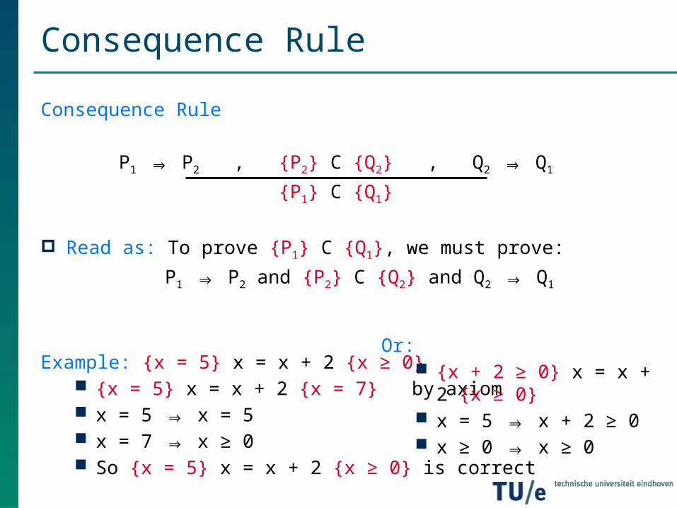
Consequence Rule

P1 ⇒ P2 , {P2} C {Q2} , Q2 ⇒ Q1

{P1} C {Q1}

Read as: To prove {P1} C {Q1}, we must prove:

P1 ⇒ P2 and {P2} C {Q2} and Q2 ⇒ Q1

Example: {x = 5} x = x + 2 {x ≥ 0} {x = 5} x = x + 2 {x = 7} by axiom x = 5 ⇒ x = 5 x = 7 ⇒ x ≥ 0 So {x = 5} x = x + 2 {x ≥ 0} is correct

Or: {x + 2 ≥ 0} x = x + 2 {x ≥

0} x = 5 ⇒ x + 2 ≥ 0 x ≥ 0 ⇒ x ≥ 0

Practice

1. {False} x = 5 {x = 6}

2. {False} x = 5 {x = 5}

3. {x ≥ 0} x = x – 2 {x – 2 ≥ 0}

4. {x = 2} x = x + y {True}

5. {x is even} x = x + 4 {x is even}

Single commands are easy…

Composition Rule

Composition Rule

{P} C1 {Q} , {Q} C2 {R}

{P} C1 ; C2 {R}

Note that Q must be chosen May require some creativity…

Example: {x = 7} y = x + 1; z = 2y + x {z = 23} Choose Q: (x = 7 and y = 8) {x = 7} y = x + 1 {x = 7 and y = 8} {x = 7 and y = 8} z = 2y + x {z = 23}

Why not Q: y = 8?

Practice

Exercise

{x = A and y = B}

1. h = x

2. x = x + y

3. y = x – y

4. h = h + x + y

5. x = x – y

6. h = (h + 2x)/3

{x = B and y = A and h = A + B}

Prove it!

Practice

Exercise

{x = A and y = B}

1. h = x

2. x = x + y

3. y = x – y

4. h = h + x + y

5. x = x – y

6. h = (h + 2x)/3

{x = B and y = A and h = A + B}

Prove it!

{x = A and y = B and h = A}

{x = A + B and y = B and h = A}

{x = A + B and y = A and h = A}

{x = A + B and y = A and h = 3A + B} {x = B and y = A and h = 3A + B}

Composing Assignments

Proofs in Data Structures

Sequences of assignments are easy to prove Simply change values while executing assignments Normally much easier than example on previous slide

In Data Structures we don’t prove much for assignments {P} C1 ;…; Cn {Q} where Ci are assignments is argued directly {P} and {Q} are mentioned and used in the remainder of the proof But the Hoare triple is assumed like an axiom

1. h = x

2. x = y

3. y = hWe simply say that x and y are swapped

Conditional Rule

Conditional Rule

{B ⋀ P} C1 {Q} , {¬B ⋀ P} C2 {Q}

{P} if B then C1 else C2 {Q}

Also works with multiple cases If there is no “else”, then we must prove: ¬B ⋀ P ⇒ Q

Example{x ≥ 0}1. if x > y2. then z = 2x 3. else z = 2y {z ≥ x + y}

Need to prove: {x > y and x ≥ 0} z = 2x {z ≥ x + y} {x ≤ y and x ≥ 0} z = 2y {z ≥ x +

y} Case analysis?

Proving conditionals

How to write down a proof for an if-statement?

{x ≥ 0}1. if x > y2. then z = 2x 3. else z = 2y {z ≥ x + y}

Theorem

If initially x ≥ 0, then after executing the above algorithm z ≥ x + y

ProofWe consider two cases:Case (1): x > y

Then z = 2x = x + x > x + y. So z ≥ x + y holds.

Case(2): x ≤ yThen z = 2y = y + y ≥ x + y. So z ≥ x + y holds.

Case analysis!

Practice

Theorem

Prove the correctness of the following algorithm

1. {1 ≤ x,y ≤ 9}

2. if (x ≤ y and x ≤ 5)3. then z = (y – x)/24. else if x ≤ y5. then z = y – x6. else z = (x – y)/27. {0 ≤ z ≤ 4}

Practice

Proof

We consider three cases:

Case (1): x ≤ y and x ≤ 5Then z = (y – x)/2. Since x ≤ y, we get that (y – x)/2 ≥ 0. Furthermore, since 1 ≤ x,y ≤ 9, we also get that (y – x)/2 ≤ 4. Thus 0 ≤ z ≤ 4 as claimed.

Case (2): x ≤ y and x > 5Then z = y – x. Since x ≤ y, we get that y – x ≥ 0. Furthermore, since x > 5 and y ≤ 9, we also get that y – x ≤ 3. Thus 0 ≤ z ≤ 4 as claimed.

Case (3): y ≤ xThen z = (x – y)/2. Similar to case (1) we get that (x – y)/2 ≥ 0 and (x – y)/2 ≤ 4. Thus 0 ≤ z ≤ 4 as claimed.

Can we assume without loss of generality that x ≤ y?

While Rule

While Rule

P ⇒ S , {S ⋀ B} C {S} , S ⋀ ¬B ⇒ Q{P} while B do C {Q}

We already know how to prove loops S is the invariant P ⇒ S is the initialization {S ⋀ B} C {S} is the maintenance S ⋀ ¬B ⇒ Q is the termination

It is hard to come up with a good invariant Therefore you must always prove it in Data Structures!

Example

BinarySearch(A, n, k)

1. {A contains n ≥ 2 integers in increasing order with A[1] ≤ k < A[n]}

2. x = 1

3. y = n

4. while x + 1 ≠ y

5. do h = (x + y)/2

6. if A[h] ≤ k7. then x = h8. else y = h9. {If A contains k, then A[x] = k}

What is the invariant?

{x = 1 and y = n and A contains…}

{Invariant}

Often part of input specification

Example

BinarySearch(A, n, k)

1. {A contains n ≥ 2 integers in increasing order with A[1] ≤ k < A[n]}

2. x = 1

3. y = n

4. while x + 1 ≠ y

5. do h = (x + y)/2

6. if A[h] ≤ k7. then x = h8. else y = h9. {If A contains k, then A[x] = k}

What is the invariant?A[x] ≤ k and A[y] > k

{x = 1 and y = n and A contains…}

{Invariant}

Often part of input specification

Example

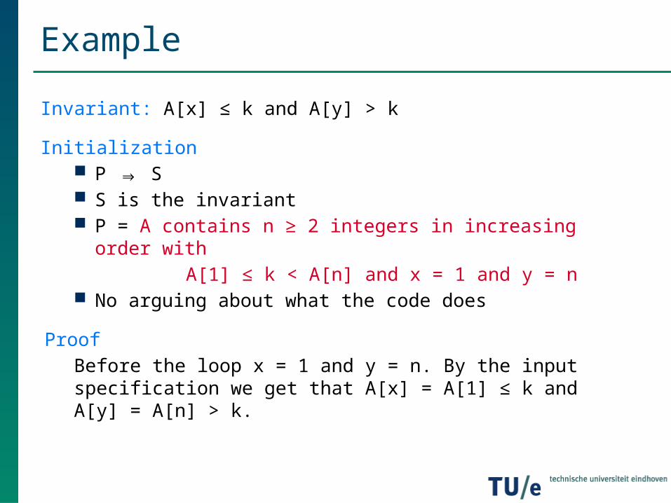
Invariant: A[x] ≤ k and A[y] > k

Initialization P ⇒ S S is the invariant P = A contains n ≥ 2 integers in increasing order with

A[1] ≤ k < A[n] and x = 1 and y = n No arguing about what the code does

ProofBefore the loop x = 1 and y = n. By the input specification we get that A[x] = A[1] ≤ k and A[y] = A[n] > k.

Example

Invariant: A[x] ≤ k and A[y] > k

Maintenance {S ⋀ B} C {S} B: x + 1 ≠ y

ProofBefore each iteration it holds that A[x] ≤ k, A[y] > k, and x + 1 ≠ y. We need to show that after the iteration A[x] ≤ k and A[y] > k. Let h = (x + y)/2. There are two cases:Case (1): A[h] ≤ k

Then x = h and y is unchanged after the iteration. So, A[x] = A[h] ≤ k, and A[y] > k by invariant.

Case (2): A[h] > kThen y = h and x is unchanged after the iteration. So, A[y] = A[h] > k, and A[x] ≤ k by invariant.

Example

Invariant: A[x] ≤ k and A[y] > k

Termination S ⋀ ¬B ⇒ Q ¬B: x + 1 = y Q = If A contains k, then A[x] = k Again no arguing about what the code does

ProofAfter the loop A[x] ≤ k, A[y] > k, and x + 1 = y. Hence, A[x] ≤ k < A[x+1].If A[x] < k, then A[x] < k < A[x+1]. Since A is sorted, A cannot contain k.Thus, if A contains k, then A[x] = k.

“A is sorted” not in invariant → we could add it… … but too cumbersome → “sloppiness” is allowed here

For Loops

How about a for loop?

Simply convert to while loop:

1. for i = 1 to n

2. do C 1. i = 1

2. while i ≤ n3. do C4. i = i + 1

P ⋀ i=1 ⇒ S , {S ⋀ i ≤ n} C {S[i+1/i]} , S ⋀ i > n ⇒ Q{P} for i = 1 to n do C {Q}

not very useful

For Loops

How about a for loop?

Simply convert to while loop:

1. for i = 1 to n

2. do C 1. i = 1

2. while i ≤ n3. do C4. i = i + 1

P ⋀ i=1 ⇒ S , {S ⋀ i ≤ n} C {S[i+1/i]} , S ⋀ i=n+1 ⇒ Q{P} for i = 1 to n do C {Q}

Termination

Termination woes

Guards like i ≤ n do not give much information (i > n) for termination Formally, we could add i ≤ n + 1 to invariant… … but that’s cumbersome

Instead we simply argue termination value(s) If obvious, no argument is needed

1. for i = n downto 1

2. do stuff 1. while x2 < n

2. do x = x + 1

1. while x ≤ n

2. do x = x + 2

Termination values?

i = 0 x = ⌈√n⌉ x = n+1 or x = n+2

Invariant vs. Induction

Invariant vs. Induction

Similarities Invariant is like Induction Hypothesis Initialization is like base case Maintenance is like induction step Proofs are very similar!

Differences Maintenance must argue about code Termination: loops terminate, induction does not

Example

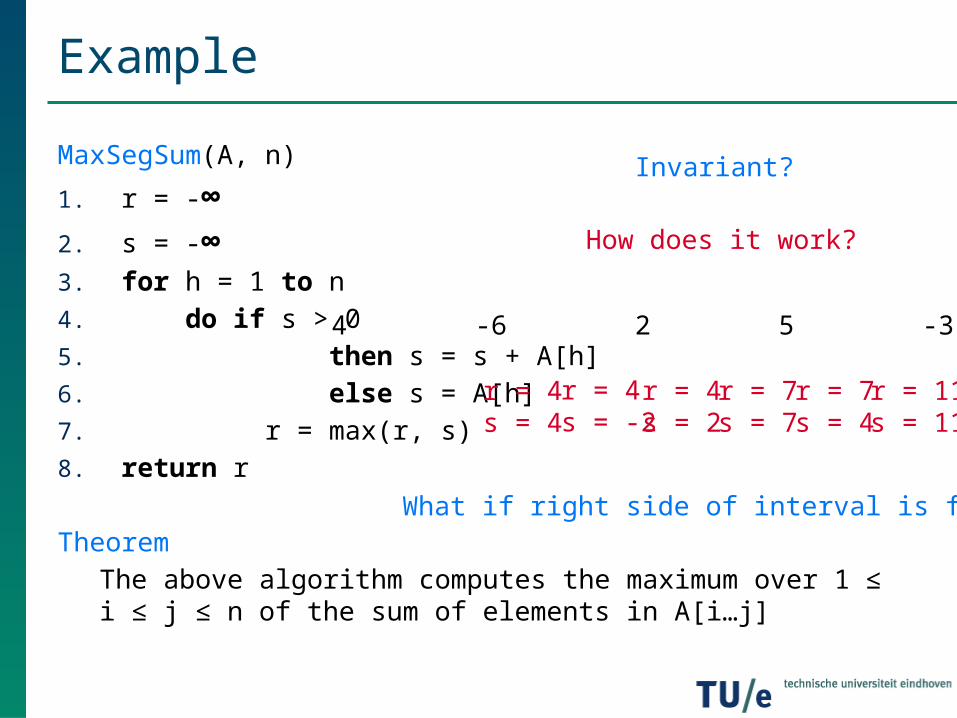
MaxSegSum(A, n)

1. r = -∞2. s = -∞3. for h = 1 to n

4. do if s > 0

5. then s = s + A[h]

6. else s = A[h]

7. r = max(r, s)

8. return r

Theorem

The above algorithm computes the maximum over 1 ≤ i ≤ j ≤ n of the sum of elements in A[i…j]

Invariant?

How does it work?

4 -6 2 5 -3 7

r = 4s = 4

r = 4s = -2

r = 4s = 2

r = 7s = 7

r = 7s = 4

r = 11s = 11

What if right side of interval is fixed?

Example

MaxSegSum(A, n)

1. r = -∞2. s = -∞3. for h = 1 to n

4. do if s > 0

5. then s = s + A[h]

6. else s = A[h]

7. r = max(r, s)

8. return r

Theorem

The above algorithm computes the maxsum of A[i…j] over

1 ≤ i ≤ j ≤ n

Invariant?

How does it work?

4 -6 2 5 -3 7

r = 4s = 4

r = 4s = -2

r = 4s = 2

r = 7s = 7

r = 7s = 4

r = 11s = 11

What if right side of interval is fixed?

Example

MaxSegSum(A, n)

1. r = -∞2. s = -∞3. for h = 1 to n

4. do if s > 0

5. then s = s + A[h]

6. else s = A[h]

7. r = max(r, s)

8. return r

Invariant

r contains the maxsum of A[i…j] over 1 ≤ i ≤ j ≤ h-1, and s contains the maxsum of A[i…h-1] over 1 ≤ i ≤ h-1

Invariant?

How does it work?

4 -6 2 5 -3 7

r = 4s = 4

r = 4s = -2

r = 4s = 2

r = 7s = 7

r = 7s = 4

r = 11s = 11

What if right side of interval is fixed?

Example

Invariant

r contains the maxsum of A[i…j] over 1 ≤ i ≤ j ≤ h-1, and s contains the maxsum of A[i…h-1] over 1 ≤ i ≤ h-1

Initialization

Before the loop, h = 1. Hence, both 1 ≤ i ≤ j ≤ h-1 and 1 ≤ i ≤ h-1 are empty domains. The maximum over an empty domain is -∞, so the invariant is correctly initialized.

Example

Invariant

r contains the maxsum of A[i…j] over 1 ≤ i ≤ j ≤ h-1, and s contains the maxsum of A[i…h-1] over 1 ≤ i ≤ h-1

Maintenance

Before each iteration the invariant holds. We need to show that after the iteration r contains the maxsum of A[i…j] over

1 ≤ i ≤ j ≤ h, and s contains the maxsum of A[i…h] over 1 ≤ i ≤ h.We consider two cases:Case (1): s > 0

Let the maxsum of A[i…h] be obtained for i = i*. Note that i* ≠ h, since the maxsum of A[i…h-1], which is stored in s by invariant and is positive, can be added to A[h…h] to get a larger sum. So, i* < h and the maxsum of A[i…h] is A[h] plus the maxsum of A[i…h-1]. By invariant, s contains the maxsum of A[i…h-1], so A[h] should indeed be added to s.

Example

Invariant

r contains the maxsum of A[i…j] over 1 ≤ i ≤ j ≤ h-1, and s contains the maxsum of A[i…h-1] over 1 ≤ i ≤ h-1

Maintenance (continued)

Case (2): s ≤ 0Again, let the maxsum of A[i…h] be obtained for i = i*. If i* < h, then the sum of A[i*…h-1] is at most s by invariant, and thus at most zero. As a result, A[i*…h] is at most A[h], which can be achieved by i* = h. Thus s should indeed be set to A[h].

After the if-statement, s contains the maxsum of A[i…h] over 1 ≤ i ≤ h. Let the maxsum of A[i…j] be obtained for j = j*. If j* = h, then s must contain the maxsum of A[i…j]. Otherwise j* < h, and r must already contain the maxsum of A[i…j] by invariant. Thus, the maximum of r and s will be the maxsum of A[i…j] over 1 ≤ i ≤ j ≤ h.

Example

Invariant

r contains the maxsum of A[i…j] over 1 ≤ i ≤ j ≤ h-1, and s contains the maxsum of A[i…h-1] over 1 ≤ i ≤ h-1

Termination

After the loop, h = n+1. By invariant, r contains the maxsum of A[i…j] over 1 ≤ i ≤ j ≤ h-1 = n. Thus, r contains the correct value.

Nested Loops

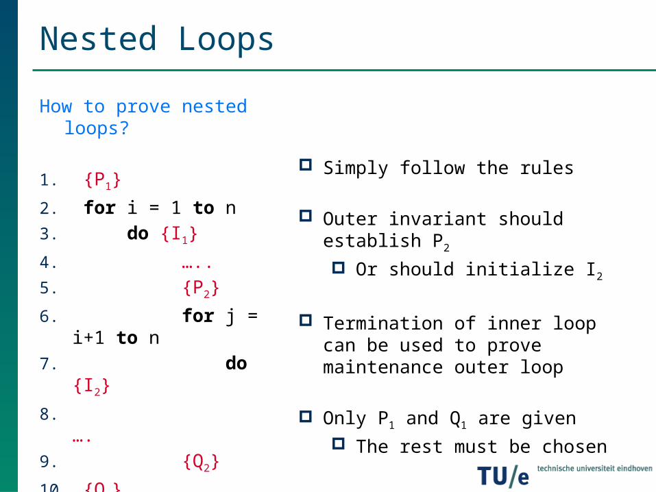
How to prove nested loops?

1. {P1}

2. for i = 1 to n

3. do {I1}

4. …..

5. {P2}

6. for j = i+1 to n

7. do {I2}

8. ….

9. {Q2}

10. {Q1}

Simply follow the rules

Outer invariant should establish P2

Or should initialize I2

Termination of inner loop can be used to prove maintenance outer loop

Only P1 and Q1 are given The rest must be chosen

Summary

Hoare logic Formal system for proving algorithms Basically defines the “rules of the game”

Proofs in Data Structures No Hoare logic! (only in the background) Assignments: generally without proof If-statements: prove using case distinction Loops: prove using loop invariant

Always make the distinction between “what the code does” and “what it is supposed to do”! The goal is to prove that these two things are the same