RUSSIAN RESEARCH CENTER THE INSTITUTE OF ECONOMIC RESEARCH

HITOTSUBASHI UNIVERSITY Kunitachi, Tokyo, JAPAN

RRC Working Paper Series No. 43 Центр Российских Исследований

Shortages and the Informal Economy In the Soviet Republics: 1965-1989

Byung Yeon Kim

Yoshisada Shida

March 2014

ISSN 1883-1656

1

Shortages and the Informal Economy

in the Soviet Republics: 1965–1989*

Byung Yeon Kim (Seoul National University)

Yoshisada Shida (Hitotsubashi University)

Abstract

We measure the informal economy and shortages of consumer goods in the

Soviet republics from 1965 to 1989 to estimate the relationships of these two

variables. We use fixed-effect model and instrument variable approach and

find that the informal economy and shortages reinforce each other. Results

indicate that the Soviet central planning system is difficult to sustain in the

long run. A substantial heterogeneity across the Soviet republics exists not

only in the extent of the informal economy and shortages, but also in the

associations of the two variables.

Keywords: shortages, informal economy, Soviet republics

JEL Codes: P21, P27, P36.

* Byung Yeon Kim, Department of Economics, Seoul National University, South Korea,

kimby@snu.ac.kr; Yoshisada Shida, Institute of Economic Research, Hitotsubashi

University, Japan, shida@ier.hit-u.ac.jp.

** We thank Ichiro Iwasaki, Masaaki Kuboniwa, and Yasushi Nakamura for their

valuable suggestions. We likewise appreciate the constructive comments and

suggestions from the participants at the Pacific Rim conference in Seoul in April 2013.

2

I. Introduction

Centrally planned economies (CPEs) are typically described as the

system in which the central planning coordinates the economic activities of

enterprises and households. Central planners draw comprehensive plans that

contain detailed information on inputs and outputs, suppliers and consumers, and

household income and the supply of consumer goods and services. Input

producers supply the required inputs and deliver them to firms according to the

plans. Goods and services produced using such inputs are supplied to consumers

as central plans dictate. Hence, shortages in the consumer markets and the

informal economy (or the so-called second economy) in the ideal type of CPEs

are marginally possible.

However, ideal CPEs were inexistent. Central planning often suffered

from inconsistency and lack of knowledge on the behavior and capacity of firms.

Central planners accused firms of attempting to hide local information on

themselves soon after the establishment of CPEs. Firm managers simultaneously

complaint that inputs required to produce outputs were not delivered, but central

planners still demanded that output targets be fulfilled. Households found that

they were unable to purchase goods in official shops and thus conducted informal

economic activities with enterprises; households and enterprises produced goods

and services informally, that is, either against laws or outside the operational

domain of central planners. Households and enterprises sold goods at markets to

earn extra income. Households sold their products from private plots at collective

farmers’ markets, which were part of informal markets. Several households

purchased goods in an official shop and resold them at higher prices in informal

markets. Enterprises bought inputs from unofficial input suppliers (talkachi) and

earned money by selling their goods at markets.

Shortages and the informal economy are the two important features of

the Soviet economy (Grossman, 1977; Treml and Alexeev, 1994; Kim, 1999;

2002). The informal economy co-existed with central planning from the

beginning of the Soviet socialism (Grossman, 1977; O’Hearn, 1980). Shortages

have prevailed in consumer markets until the dissolution of the Soviet Union

(Kim, 1999; 2002). The disequilibrium school argues that shortages could reduce

labor supply because households facing shortages attempt to substitute money

with leisure. A vicious circle is consequently generated because reduced labor

supply implies reduced supply of consumer goods, which further intensifies

3

shortages. This argument indicates that CPEs suffering from shortages in the

consumer market are inherently unstable and destined to collapse. However,

several studies have argued that workers have difficulty in reducing working

hours freely in the centralized Soviet system that is characterized by heavy

regulations and harsh penalties (Howard, 1976). Furthermore, the informal

economy helps keep the value of money; households can buy goods informally,

although the official market has shortages of these goods (Alexeev, 1988).

Shortages and the informal economy have been studied separately; no

research has analyzed the relationship between these two variables. Do these two

variables reinforce each other and cause a vicious circle in CPEs? Alternatively,

do they interact to produce a stable equilibrium? These questions are important

for understanding the stability of CPEs. Moreover, the Soviet republics may have

been different in terms of the extent of shortages and the informal economy, and

the relationship of these two variables. The presence of heterogeneity has

implications for the collapse of the Soviet economy.

We aim to contribute to the literature in two aspects. First, using

previously unavailable archival material, we extend the estimates of Kim (1999;

2003) of the informal economy in the Soviet Union as a whole from 1965 to 1989

to all 15 Soviet republics in the same period. We combine these data with the

measures of shortages and other variables at the republic level. Second, we

estimate the determinants of the informal economy and shortages simultaneously

as well as independently to understand the relationship between these two

factors.

We find that shortages increase the informal economy and that the

informal economy intensifies shortages. These positive relationships between

these variables suggest that CPEs are an unstable system; the planned official

sector shrinks in the long run as informal markets replace the planned sector. Yet,

a large heterogeneity exists in the informal economy and shortages among Soviet

republics. In particular, the informal economy and shortages interacted more

intensively in Russia and Ukraine than in republics in Central Asia.

This paper is organized as follows. In Section II, we review the related

literature. In Section III, we measure the informal economy using the material

from Russian archives. In Section IV, we estimate the determinants of the

informal economy and shortages in reduced and structural forms. In Section V,

we summarize our findings and discuss their implications.

4

II. Literature Review

The Soviet informal economy (i.e., the second economy) began to be

discussed in the literature following the pioneering work of Grossman (1977).1

Grossman defined the second economy as a platform for “all production and

exchange activities that fulfill at least one of the two following tests: (a) they

intended directly for private gain; (b) they were conducted in some significant

respect with understanding they were in contravention of existing law.”

Grossman estimated the amount of goods and services transacted in the informal

economy. Afterwards, several related studies on the Soviet informal economy

have been conducted mainly by Western researchers (Schroeder and Greenslade,

1979; O’Hearn, 1980; Ericson, 1983; Brezinski, 1985; Cassel and Cichy, 1986).

The principal interests of these studies include the definition, the size of the

informal economy, its causes and effects, and the classification of activities.

However, their analyses are limited to describing the typologies and working

mechanisms of informal economy, and providing rough estimations based on

anecdotal evidence that appeared in Soviet newspapers and journal articles.2

The Soviet Interview Project and the Berkeley-Duke Émigré Survey

collected data on the Soviet informal economy from Soviet immigrants in Israel

and the United States in the 1970s, respectively; they substantially improved data

availability and analytical rigor. Nevertheless, they suffered from problems

arising from a non-representative sample. Although Soviet researchers began to

pay attention to its second economy prior to the collapse of the regime, their

work failed to provide reliable estimates of the second economy (Осипенко,

1989; Головнин and Шохин, 1990; Корягина, 1990). More reliable estimates

were obtained because of the availability of previously classified data after the

collapse of the Soviet Union. Kim (2003) used previously unpublished archival

material of household budget surveys and classified the informal economy into

three types, namely, informal production, illegal production, and rent-seeking

activities. Kim reported that the latter two tended to increase during the period of

Perestroika. Shida (2011) confirmed this finding at the republic level.

Several researchers have examined the effects of the informal economy

on the entire economy to understand whether the informal economy stabilizes or

1 Hereafter, we use “informal” and “second” economy interchangeably. 2 Schroeder and Gleenslade (1979) and Rutgaizer (1992a; 1992b) reviewed the Soviet literature that contains information on the size of the second economy.

5

destabilizes the entire economy (Ericson, 1983; Cassel and Cichy, 1986; Galasai

and Sik, 1988; Alexeev, 1988; Treml and Alexeev, 1994). The informal economy

may affect the economy positively. It increases price flexibility, which drives the

price of a good closer to its scarcity. It simultaneously eases inflationary

pressures in the official market by absorbing a part of unspent money in the

official economy, and reduces the supply multiplier, that is, the tendency of

households to substitute money income with leisure when they are frustrated

about the inability to purchase goods and services in the official economy.

However, O’Hearn (1980) and Treml and Alexeev (1994) argued that the effect of

the informal economy is detrimental. O’Hearn (1980) suggested that the role of

the informal economy in the economy as a whole can be supplementary, depletive,

or redistributive, depending on its characteristics. Following this line of approach,

Treml and Alexeev (1994) indicated that an increase in the informal economy

beyond a certain threshold could destabilize the official economy.

Early empirical studies on shortages in Soviet consumer markets have

failed to find any evidence of shortages (Pickersgill, 1976; Ofer and Pickersgill,

1980). However, these studies suffered from data unavailability, measurement

errors, and methodological problems arising from the non-stationarity of

variables. Kim (1997; 2002) and Asgary et al. (1997) provided more reliable

evidence of shortages in Soviet consumer markets.

Previous studies have failed to explore the shortage factor in considering

the effect of the informal economy on the official economy. The disequilibrium

model analyzes the relationship between shortages and the official economy, but

failed to include the informal economy in its model (Davis and Charemza, 1989).

The informalization hypothesis maintains that the Soviet economy collapsed

because of its informalization, that is, the replacement of the official economy

with the informal economy and its association with corruption and deterioration

of support for socialist norms (Treml and Alexeev, 1994; Grossman, 1998).

However, these studies have investigated only the relationship between the

official and the informal economy, although the dynamics of the informal

economy may have been associated with shortages.3

The informal economy is likely to interact with shortages in the official

economy. An increase in the total supply of goods and services due to the

existence of the informal economy could reduce shortages in the official

3 Queue-rationing mechanism in the official and parallel markets is formally discussed in the literature (Stahl and Alexeev, 1989).

6

economy because household demand for goods and services in the official sector

decreases. In more detail, households may work harder in the informal economy

than in the official one, which increases the total supply of consumer goods and

services available in the economy. Furthermore, the informal economy where

prices are determined freely by supply and demand can absorb at least part of

shortages in the official economy. These conjectures imply that shortages in the

official economy decrease as those in the informal economy increase. However,

using inputs taken away from the official economy for production in the informal

economy intensifies shortages in the informal economy. In addition, firms prefer

to sell their produced goods and services in the informal economy to increase

profit (Harrison and Kim, 2006). Moreover, households accumulate money from

activities in the informal economy and may use it in the official economy. Hence,

an alternative conjecture can be established in that the informal economy

intensifies shortages.

In sum, the issues of whether the net effect of the informal economy on

shortages is positive or negative, and whether the development of the informal

economy is stimulated by the intensified shortages remain unclear. These

unresolved questions on the dynamic relationships between the informal

economy and shortages are empirically examined in the subsequent sections.

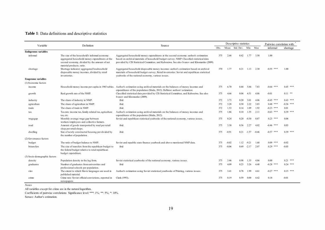
III. Data

This section measures the informal economy and shortages at the level of

the Soviet republics, and introduces various independent variables to estimate the

relationships between the informal economy and shortages. We use declassified

archival materials on household budget surveys from RGAE (Российский

государственный архив экономики) to estimate the size of the informal

economy and reconstruct our statistical database of household incomes,

expenditures, and items traded by the republics. According to Kim (2003), the

informal economy has three components, namely, the self-consumption of

agricultural products, trading between citizens, and redistribution among citizens.

We use only the second and third components to measure the informal economy

to understand its relationship with shortages because the self-consumption of

agricultural products is closely associated with the stage of economic

7

development.4 The share of the informal economy (informal) refers to the ratio

of the aggregated amount of the money expenditures of households at the

informal market to the net material products (NMPs) of each republic.

Second, following Chawluk and Cross (1997), and Kim (2002), the

shortage indicator (shortage) is defined as the ratio of household disposable

money income to retail inventories at the state and cooperative retail networks.

This indicator is the only one that allows comparison across republics. Kornai

(1976) and Asgary et al. (1997) use alternative shortage indicators, for instance,

the lengths of waiting lists and queues for scarce goods and evaluations of the

goods availability collected through sample survey; however, these data are

difficult to obtain for the long period and for every republic. We present the trend

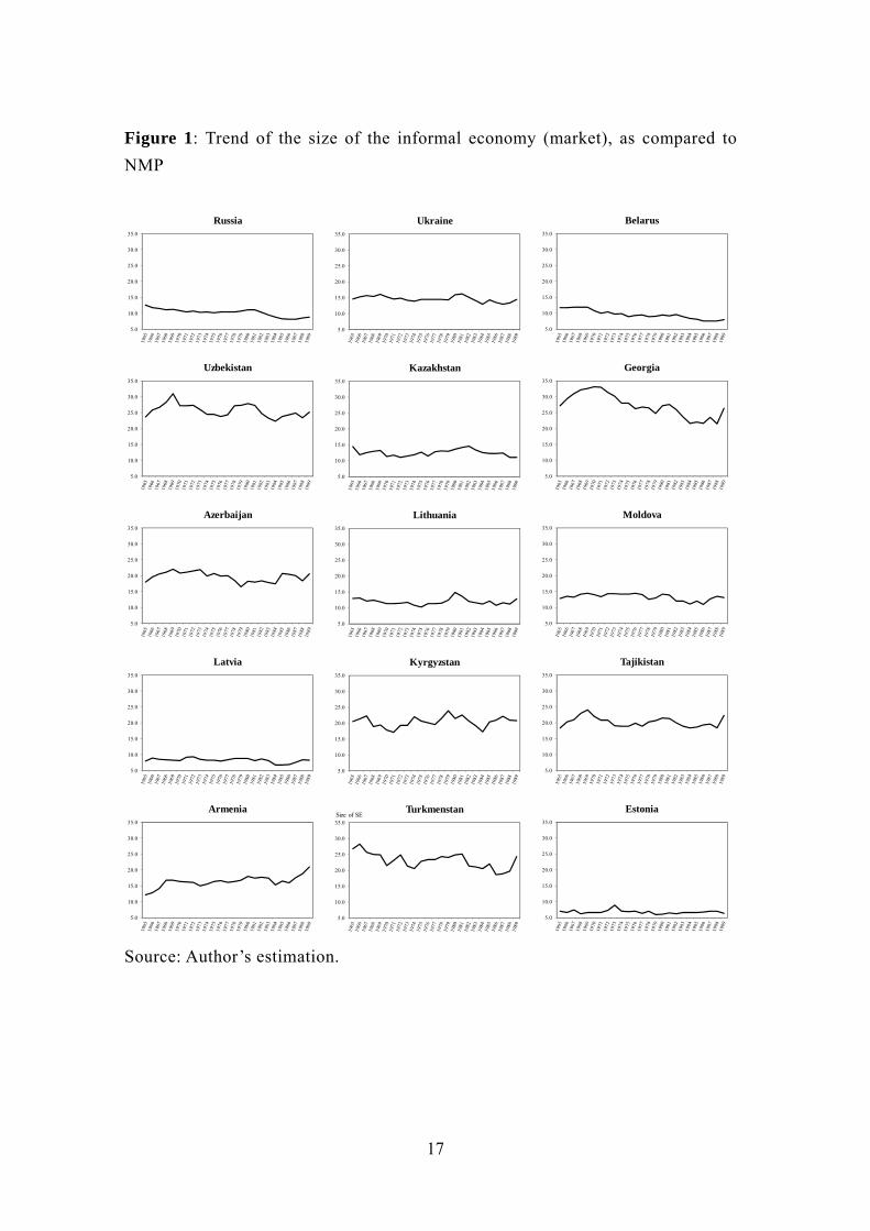
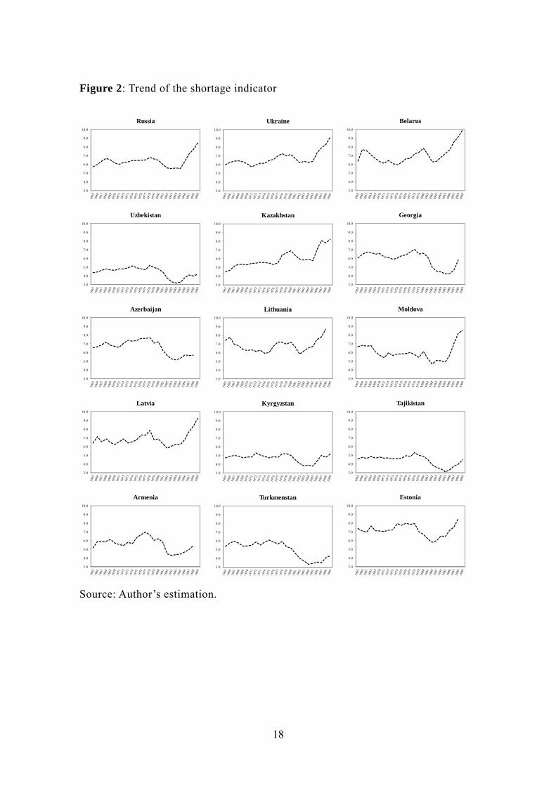
of the informal economy and shortages at the Soviet republics in Figures 1 and 2.

The figures show a large heterogeneity across republics in the informal economy

and shortages. For example, Figure 1 shows that the informal economy is much

larger in Central Asia and Caucasian republics but relatively smaller in Baltic

republics. In contrast, the shortage patterns across republics are difficult to

characterize.

In our estimations, we use the above-mentioned dependent variables

transformed into the natural logarithm and control various factors that may affect

the informal economy and/or shortages. Conventional control (exogenous)

variables introduced capture the economic, governance, and socio-demographic

features (human capital, ethnicity, and crime) of the republics. Moreover, we

introduce the following economic variables: real economic growth rate in the log

form (official growth rate of the NMP evaluated in constant prices: growth);

industrial structure, namely, the shares of industry (industry), agriculture

(agriculture), and domestic trade, including food services (trade) in NMP;

average official income level in real terms in the log form (income); tax rate for

household in the log form (tax); income gap between workers/employees and

collective farmers in the log form (wagegap);5 road is the amount of goods

transported by road divided by the number of retail shops; and housing condition

4 Redistribution among citizens denotes the repayment of debts and loans borrowed from citizens. We assume that these debts and loans were mainly used for trading between citizens and constituted a part of informal financial services. 5 High income gap may stimulate trade between high- and low-income groups. That is, the high-income group intends to purchase goods in the informal economy instead of queuing in the official shops, whereas the low-income group waits in a queue to take advantage of lower prices in the official shops.

8

(dwelling), which is the size of newly constructed housing divided by the number

of population (m2 per person).

The second group of variables is classified as governance factors. We use

two variables, budget and btransfers. The former captures the governance

stability of the republic from the viewpoint of the size of the budget balance

(budget revenues minus budget expenditures) of the republic relative to NMP.

The latter variable refers to the size of transfers from the republican budget to the

federal budget relative to total budget expenditures.

With regard to social and demographic factors, we utilize population

density in the log form (persons per km2: density), and the number of graduates

per population in the log form (graduates) is included as a proxy for the level of

education in the republic. In less developed countries, people with less education

often have difficulty in finding jobs in the official labor market and thus are

forced to work informally. We also control for the ethnic factor: “slavification”

index in the log form (slav) based on the extent to which Slavic languages

(Russian, Ukrainian, and Belarusian) are used in published materials, such as

books, journals, and newspapers.6 This index captures the distance between

central control (government) and local independence (community). Local

networks may have incentives to protect illegal networks from central

investigation. In addition, non-Russian culture indicates the prevalence of a more

traditional lifestyle connected to the informal sector. The last control variable is

the reported crime per population rate (crime) derived from Clark (1993).

Variables employed in estimations and their descriptive statistics are shown in

Table 1.

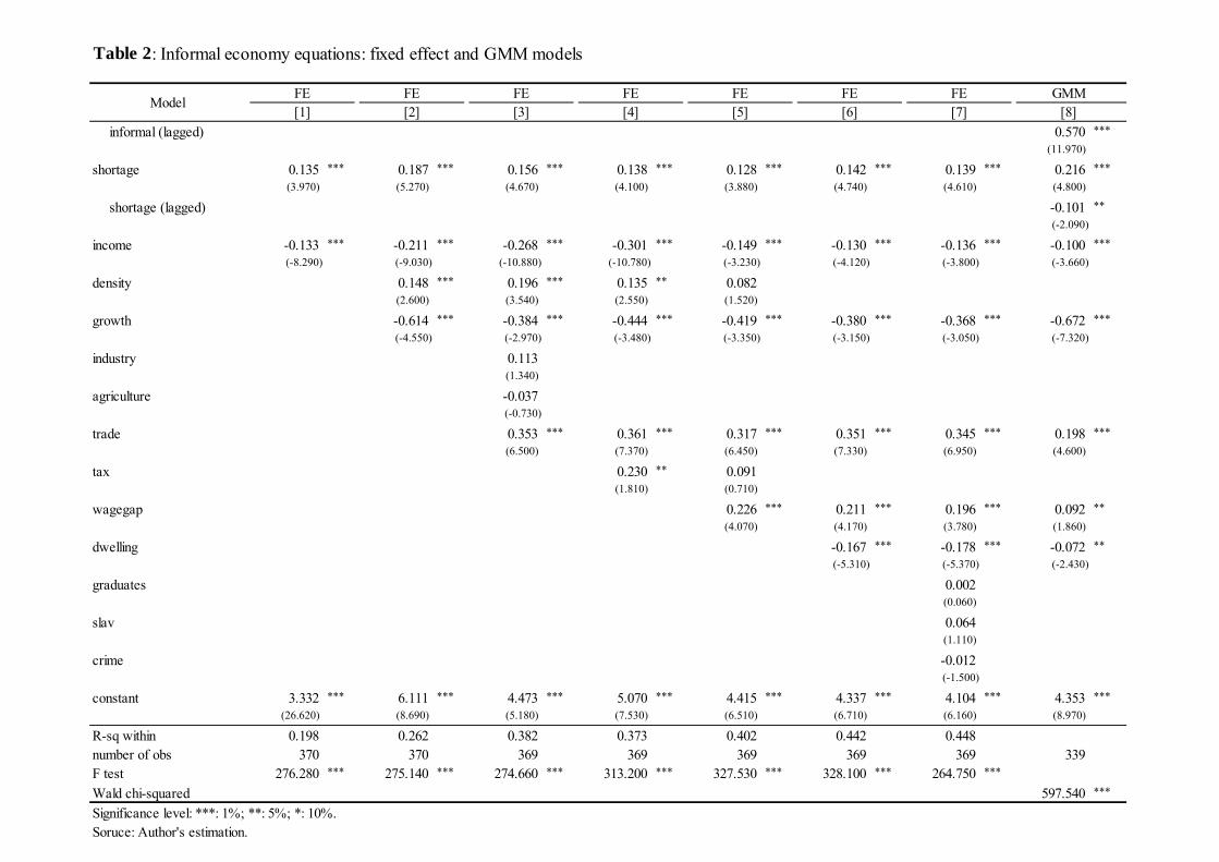
IV. Estimation Results

We first estimate the equation for the informal economy and one for

shortages separately using fixed-effect model.7 In doing so, we introduce control

variables step by step to check the significance and the robustness of our key

variables, that is, shortages in the equation for informal economy, and the

6 A similar concept, the “Russification” is presented by Anderson and Silver (1983), which emphasizes the Russian ethnicity. In our examination, Russian, Ukrainian, and Belarussian ethnicities are considered as almost the same ones. 7 Pooling regression models using Ordinary Least Squares are rejected, and fixed-effect models are preferred for both the equation for the informal economy and one for shortages.

9

informal economy in the equation for shortages. Fixed-effect model can

successfully control for time-invariant factors that affect the dependent variable

by transforming variables to deviations from the average within the unit, and thus

help avoid endogeneity problems caused by omitted fixed effects. Moreover, the

reverse causality from the dependent variable to control for variables can be

reduced using fixed-effect estimations because they exploit within-group

variation over time but do not use across-group variation that may reflect omitted

variable bias. The results obtained using fixed-effect model are presented in

Models 1 to 7. Furthermore, we use the system Generalized Methods of Moments

(GMM) estimator in Model 8. The system GMM estimator controls for both

republic-specific heterogeneity and potential endogeneity bias by combining in a

system the original specification expressed in first-differences and levels and

uses internal instruments, such as those based on the lagged values of

endogenous explanatory variables.

Table 2 shows the results of estimations for the informal economy. The

most important result is that the key variable, shortage, is positive and

statistically significant at the 1% level in all models. This result indicates that

shortages cause the informal economy to increase. Furthermore, the coefficient

on shortages changes slightly, although we introduced economic variables in

Models 2 to 6, and social and demographic variables in Model 7. Hence, the

effect of shortages on the informal economy is independent of other confounding

factors. These findings are likewise confirmed by the dynamic linear model using

the GMM with one lag displayed in Model 8.

With regard to control variables, coefficients on real income are negative

and statistically significant at the 1% level in all of the models. This finding

suggests that the Soviet informal economy is associated with the motivation of

households to earn extra income when the official income is low. This finding is

likewise supported by the negative correlation of growth with the informal

economy. The share of the trade industry in NMP is positively associated with the

informal economy. In contrast, the shares of industry (mining and manufacturing)

and agriculture in NMP are not statistically significant. These results imply that

the Soviet informal economy has closer associations with trade sectors than the

other ones. Finally, evidence suggests that income differences between the

workers/employees and collective farmers (kolkhozniki) positively influence the

informal economy.

10

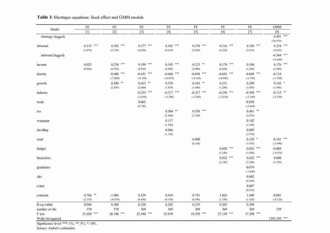
We subsequently estimate the equation for shortages using fixed-effect

models. The results are presented in Table 3. The coefficients on informal are

positive and statistically significant at the 1% level in all of the models. This

finding suggests that an increase in the informal economy intensifies shortages in

the official economy. Hence, the informal economy fails to stabilize the national

economy as argued by several studies, such as Ericson (1983), Cassel and Cichy

(1986), Sampson (1986), and Galasi and Sik (1988). Rather, it destabilizes the

economy by increasing shortages.

Coefficients on real income are positive and statistically significant at

less than the 5% level in all of the models, excluding Models 1 and 7. In other

words, the higher household income is, the more shortages in the official sector.

Population density is negatively correlated with shortages. This finding can be

explained by the higher prioritization for the supply of consumer goods of large

cities with a high population density according to the Soviet central planning. In

contrast to the finding from the informal economy equations, economic growth

increases shortages; thus, demand pressure induced by high growth is larger than

the positive effect of growth on the supply of consumer goods. The dominance of

the heavy industry in Soviet growth may account for this result. Furthermore, the

industrial structure matters because the share of the mining and manufacturing

industry in NMP is positive and statistically significant at the 1% level. With

regard to governance variables, budget balance and transfers from the republic

budget to the federal budget are likewise positive and statistically significant at

the 1% level in Models 6 and 7.8 These findings are generally supported by the

GMM estimation in Model 8.

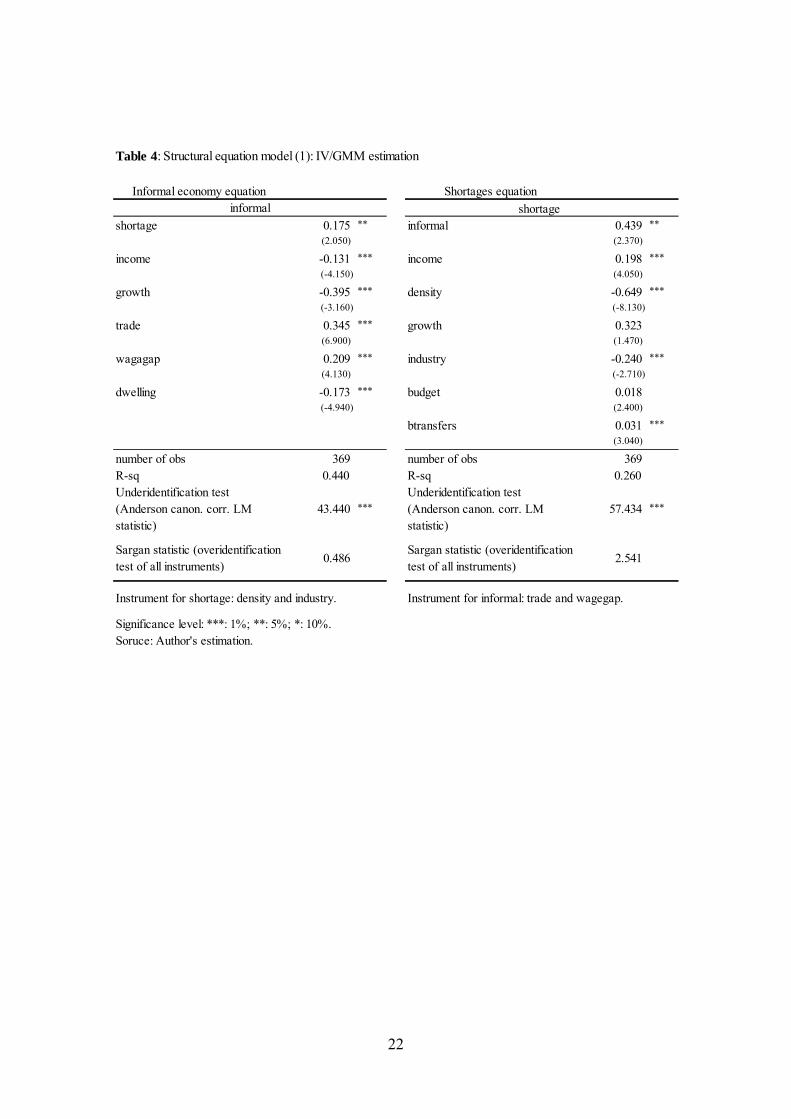
We check the robustness of the preceding results using two methods, the

instrument variable (IV) approach and structural equation approach. The IV

approach endogenizes shortages and the informal economy using external

instruments. We use two instruments for shortages, namely, population density

(density) and the share of industrial production in NMP (industry). That is, we

assume that these two instruments are exogenous to but account for the shortages

of consumer goods. We likewise use two instruments for the informal economy,

namely, wage gap between the workers/employees and the collective farmers

8 We likewise examine the effects of budget-related variables on the informal economy. These two variables are not statistically significant in all of the models and thus omitted from our estimation results.

11

(wagegap) and the share of trade in NMP (trade). The diagnostics of Tables 4 and

5 suggest that the instruments are relevant and exogenous.

The results from the equation for the informal economy, reported in

Table 4 (on the left-hand side), are similar to those in Table 2. Shortages affect

the informal economy positively. The results regarding control variables are

similar as well. Moreover, we find comparable results on the effect of the

informal economy on shortages reported in Table 4 (on the right-hand side). Our

key result of the positive association between the informal economy and

shortages remain unchanged.

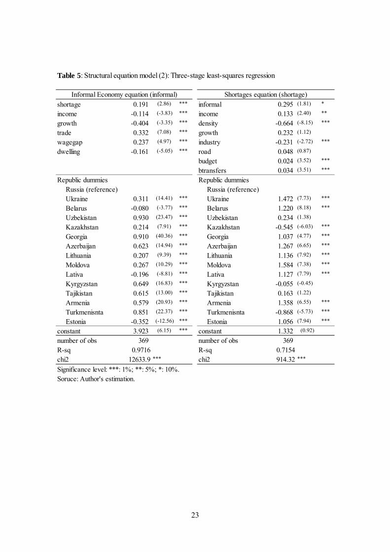
We further estimate both equations using a structural equation model in

which both the informal economy and shortages are estimated simultaneously.

The results are presented in Table 5. Both key variables are highly significant and

positive in determining the other. This finding suggests that, by reinforcing each

other, these two variables generate a vicious circle to the official economy and

destabilize the Soviet system. These built-in destabilizing factors indicate the

high instability of the Soviet economic system.

To analyze heterogeneity across the Soviet republics, we examine

regional differences in the effects of shortages and the informal economy on the

economy using a structural equation model with the republics dummies. The

results in the left-hand side of Table 5 suggest that after controlling for standard

explanatory variables, Uzbekistan and Georgia had the largest informal economy,

followed by Turkmenistan, and the other Caucasian and Central Asian republics.

In contrast, Estonia, Latvia, and Belarus had a relatively small informal economy.

The right-hand side of Table 5 shows that shortages, which were unaccounted for

by standard variables, were the most severe in Moldova, Ukraine, and Armenia,

but households in Central Asia and Russia suffered from shortages to a lesser

extent.

We further investigate the relationships between the informal economy

and shortages using regional dummies and interaction terms. Each republic is

clustered to the following regions: Slavic region as a reference group (comprising

Russia, Ukraine, Belarus, and Moldova); Central Asia (Uzbekistan, Kazakhstan,

Kyrgyzstan, Tajikistan, and Turkmenistan); Caucasus (Georgia, Azerbaijan, and

Armenia); and Baltic region (Lithuania, Latvia, and Estonia). The estimation

results confirm the regional variations of shortages and the informal economy.

The largest informal economy is found in Central Asian and Caucasian republics,

12

followed by Baltic and European republics; meanwhile, shortages are more

severe in Baltic and Caucasian republics.

The results in Table 6 can be used to understand the relationships

between the informal economy and shortages that vary across the clustered

regions. The magnitude of the effects of shortages on the informal economy can

be computed by adding the coefficient on shortages in the informal economy

equation to those on the interaction terms between regional dummies and

shortages in the same equation. Similarly, we can compute the magnitude of the

effects of informal economy on shortages by adding the coefficient on the

informal economy in the shortage equation to those on the interaction terms

between regional dummies and shortages in the same equation. The results are

summarized in Table 7. All of the coefficients have positive signs and are

statistically significant at least at the 5% level. The most important finding is that

reference regions, that is, European regions, had the strongest spillover both from

shortages to the informal economy and from the informal economy to shortages.

The second strongest spillover effects are found in Baltic republics. However, the

gaps in the magnitude of such effects between European regions and the other

regions, including Baltic ones, are substantially large. These results imply that

the official economy in European regions was hit hardest by the vicious circle

generated by shortages and the informal economy in these regions. Hence, these

regions had arguably the most vulnerable central planning system and may have

had the strongest public support for changes in the economic system. This finding

can explain why the Russian public supported the transition toward a market

economy in the early 1990s, which terminated the Soviet economic system.

V. Conclusion

This study measures the informal economy and shortages of consumer

goods from 1965 to 1989 at the level of the Soviet republics to estimate the

relationships between these two variables. We apply fixed-effect estimator,

instrumental variable approach, and structural estimator to these data.

The informal economy and shortages positively affect each other. In

other words, the informal economy intensifies shortages in the official economy,

whereas shortages increase activities in the informal economy. Thus, sustaining

the Soviet economic system based on central planning is difficult in the long run.

The shortages of consumer goods were caused not by policy mistakes but by

13

structural problems in the CPE. Similarly, activities in the informal economy

emerged as a result of inherent problems in the Soviet economic system. The

positive association of the informal economy and shortages indicates the

existence of a vicious circle in the system.

A substantial heterogeneity likewise exists not only in the extent of

shortages and the informal economy across the Soviet republics, but also in the

relationships between these two variables. The results suggest that the official

economy of the European regions, including Russia, Ukraine, Belarus, and

Moldova, was hit hardest by the vicious circle generated by the positive

interaction between shortages and the informal economy. This outcome explains

why the Russian public supported Yeltsin, who decided to make a transition

toward a market economy.

14

References

Alexeev, M. (1988), “Are Soviet Consumer Forced to Save?” Comparative

Economic Studies, Vol. 30, No. 4, pp. 17-23.

Anderson, B. and B. Silver (1983), “Estimating Russification of Ethnic Identity

among Non-Russians in the USSR,” Demography, Vol. 20, No. 4, pp.

461-489.

Asgary, N., P. Gregory, and M. Mokhtari (1997), “Money Demand and Quantity

Constraints: Evidence from the Soviet Interview Project,” Economic

Inquiry, Vol. 35, pp. 365-377.

Brezinski, H. (1985), “The Second Economy in the Soviet Union and Its

Implication for Economic Policy.” In: W. Gaertner and A. Wenig (eds.), The

Economics of the Shadow Economy, Proceedings of the International

Conference on the Economics of the Shadow Economy Held at the

University of Bielefeld, West Germany October 10-14, 1983, pp. 362-391.

Cassel, D. and E. Cichy (1986), “Explaining the Growing Shadow Economy: A

Comparative Systems Approach,” Comparative Economic Studies, Vol. 28,

No. 1, pp. 20-41.

Chawluk, A. and R. Cross (1997), “Measures of Shortage and Monetary

Overhang in the Polish Economy,” Review of Economics and Statistics, Vol.

79, No. 1, pp. 105-115.

Clarke, W. (1993), “Crime and Punishment in Soviet Officialdom,” Europe-Asia

Studies, Vol. 45, No. 2, pp. 259-279.

Davis, C. and Charemza, W., eds. (1989), Models of Disequilibrium and Shortage

in Centrally Planned Economies,London and New York: Chapman and Hall.

Galasi, P. and E. Sik (1988), “Invisible Incomes in Hungary,” Social Justice, Vol.

15, No. 3-4, pp. 160-178.

Grossman, G. (1977), “The Second Economy of the USSR,” Problems of

Communism, Sept.-Oct., pp. 25-40.

Grossman, G. (1998), “Subverted Sovereignty: Historic Role of the Soviet

Underground.” In:S. Cohen, A. Schwartz, and J. Zysman (eds.), The Tunnel

at the End of the Light: Privatization, Business Networks, and Economic

Transformation in Russia, Berkeley: University of California, pp. 24-50.

Ericson, R. (1983), “On an Allocative Role of the Soviet Second Economy.” In:P.

Desai (ed.), Marxism, Central Planning and the Soviet Economy,

Cambridge, M.A.: MIT Press.

15

Harrison, M. and B.Y. Kim (2006), “Plans, Prices, and Corruption: The Soviet

Firm under Partial Centralization, 1930 to 1990,” Journal of Economic

History, Vol. 66, pp. 1-41.

Howard, D. (1976), “The Disequilibrium Model in a Controlled Economy: An

Empirical Test of the Barro-Grossman Model,” American Economic Review,

Vol. 66, No. 5, pp. 871-879.

Ivanov, Yu. and T. Khomenko (2009), “A Retrospective Analysis of the Economic

Development of Countries of the Commonwealth of Independent States,”

RRC Working Paper Series, No. 17, Institute of Economic Research,

Hitotsubashi University.

Kim, B.Y. (1997), “Soviet Household Saving Function,” Economics of Planning,

Vol. 30, pp. 181-203.

Kim, B.Y. (1999), “The Income, Savings, and Monetary Overhang of Soviet

Households,” Journal of Comparative Economics, Vol. 27, pp. 644-668.

Kim, B.Y. (2002), “Causes of Repressed inflation in the Soviet Consumer Market,

1965-1989: Retail Price Subsidies, the Siphoning Effect, and the Budget

Deficit,” Economic History Review, Vol. 55, No. 1, pp. 105-127.

Kim, B.Y. (2003), “Informal Economic Activities of Soviet Households: Size and

Dynamics,” Journal of Comparative Economics, Vol. 31, No. 3, pp.

532-551.

Kornai, J. (1976), “The Measurement of Shortage,” Acta Oeconomica, Vol. 16,

No. 3-4, pp. 321-344.

Ofer, G. and J. Pickersgill (1980), “Soviet Household Saving: A Cross-section

Study of Soviet Emigrant Families,” Quarterly Journal of Economics, Vol.

95, pp. 121-44.

O’Hearn, D. (1980), “The Consumer Second Economy: Size and Effects,” Soviet

Studies, Vol. 32, No. 2, pp. 218-234.

Pickersgill, J. (1976), “Soviet Household Saving Function,” Review of Economics

and Statistics, Vol. 58, pp. 139-47.

Rutgaizer, V. (1992a), “The Shadow Economy in the USSR: A Survey of Soviet

Research,” Berkeley-Duke Occasional Papers, No. 34, Part 1.

Rutgaizer, V. (1992b), “Sizing Up the Shadow Economy: Review and Analysis of

Soviet Estimates,” Berkeley-Duke Occasional Papers, No. 34, Part 2.

Sampson, S. (1986), “The Informal Sector in Eastern Europe,” Telos, Vol. 66, pp.

44-66.

16

Schroeder, G. and R. Greenslade (1979), “On the Measurement of the Second

Economy in the USSR,” The ACES Bulletin, Vol. 21, No.1, pp. 3-22.

Shida, Y. (2011), “The Second Economy in the Soviet Republics, 1969–1988: A

New Estimation,” Slavic Studies, No. 58, pp. 123-157. (in Japanese)

Shida, Y. (2012), “Household Money Income and Expenditure in the Soviet

Republics: Re-estimation, 1960-1989,” Japanese Journal of Comparative

Economics, Vol. 49, No. 1, pp. 45-57. (in Japanese)

Stahl, L. and M. Alexeev (1985), “The Influence of Black Markets on a

Queue-Rationed Centrally Planned Economy,” Journal of Economic Theory,

Vol. 34, pp. 234-250.

Treml, V. and M. Alexeev (1994), “The Growth of the Second Economy in the

Soviet Union and Its Impact on the System.” In: Robert W. Campbell (ed.),

The Postcommunist Economic Transition: Essays in Honor of Gregory

Grossman, Boulder, Colo.: Westview Press, pp. 221-247.

Головнин, С. и А. Шохин (1990), Теневая экономика: за реализм оценок,

Коммунист, №1, С. 51-57.

Корягина, Т. (1990), Теневая экономика в СССР (анализ, оценики, прогнозы),

Вопросы экономики, №3, С. 110-120.

Осипенко, О. (1989), К анализу феномена «черного рынка», Экономические

науки, №8, С. 67-77.

17

Figure 1: Trend of the size of the informal economy (market), as compared to

NMP

Source: Author’s estimation.

5.0

10.0

15.0

20.0

25.0

30.0

35.0

Russia

5.0

10.0

15.0

20.0

25.0

30.0

35.0

Ukraine

5.0

10.0

15.0

20.0

25.0

30.0

35.0

Belarus

5.0

10.0

15.0

20.0

25.0

30.0

35.0

Uzbekistan

5.0

10.0

15.0

20.0

25.0

30.0

35.0

Kazakhstan

5.0

10.0

15.0

20.0

25.0

30.0

35.0

Georgia

5.0

10.0

15.0

20.0

25.0

30.0

35.0

Azerbaijan

5.0

10.0

15.0

20.0

25.0

30.0

35.0

Lithuania

5.0

10.0

15.0

20.0

25.0

30.0

35.0

Moldova

5.0

10.0

15.0

20.0

25.0

30.0

35.0

Latvia

5.0

10.0

15.0

20.0

25.0

30.0

35.0

Kyrgyzstan

5.0

10.0

15.0

20.0

25.0

30.0

35.0

Tajikistan

5.0

10.0

15.0

20.0

25.0

30.0

35.0

Armenia

5.0

10.0

15.0

20.0

25.0

30.0

35.0

TurkmenstanSize of SE

5.0

10.0

15.0

20.0

25.0

30.0

35.0

Estonia

18

Figure 2: Trend of the shortage indicator

Source: Author’s estimation.

3.0

4.0

5.0

6.0

7.0

8.0

9.0

10.0

Russia

3.0

4.0

5.0

6.0

7.0

8.0

9.0

10.0

Ukraine

3.0

4.0

5.0

6.0

7.0

8.0

9.0

10.0

Belarus

3.0

4.0

5.0

6.0

7.0

8.0

9.0

10.0

Uzbekistan

3.0

4.0

5.0

6.0

7.0

8.0

9.0

10.0

Kazakhstan

3.0

4.0

5.0

6.0

7.0

8.0

9.0

10.0

Georgia

3.0

4.0

5.0

6.0

7.0

8.0

9.0

10.0

Azerbaijan

3.0

4.0

5.0

6.0

7.0

8.0

9.0

10.0

Lithuania

3.0

4.0

5.0

6.0

7.0

8.0

9.0

10.0

Moldova

3.0

4.0

5.0

6.0

7.0

8.0

9.0

10.0

Latvia

3.0

4.0

5.0

6.0

7.0

8.0

9.0

10.0

Kyrgyzstan

3.0

4.0

5.0

6.0

7.0

8.0

9.0

10.0

Tajikistan

3.0

4.0

5.0

6.0

7.0

8.0

9.0

10.0

Armenia

3.0

4.0

5.0

6.0

7.0

8.0

9.0

10.0

Turkmenstan

3.0

4.0

5.0

6.0

7.0

8.0

9.0

10.0

Estonia

19

Table 1: Data definitions and descriptive statistics

Obs. Mean Std. Dev. Min Max

Endogenous variables

informal The size of the household's informal economy:aggregated household money expenditures at thesecond economy, divided by the amount of netmaterial products; ratio.

Aggregated household money expenditures at the second economy: author's estimationbased on archival materials of household budget survey; NMP: Classified statistical dataprovided by CIS Statistical Committee, and Kuboniwa. See also Ivanov and Khomenko (2009).

375 2.68 0.42 1.77 3.50 1.00

shortage Shortage indicator: aggregated houhoseholddisposable money incomes, divided by retailinventories.

Aggregated household disposable money incomes: author's estimation based on archivalmaterials of household budget survey; Retail inventories: Soviet and republican statisticalyeabooks of the national economy, various issues.

370 1.77 0.21 1.13 2.30 -0.55 *** 1.00

Exogenous variables

(1) Economic factors

income Household money income per capita in 1965 rubles. Author's estimation using archival materials on the balances of money incomes andexpenditures of the population (Shida, 2012). Deflator: authors' estimation.

375 6.70 0.44 5.84 7.83 -0.64 *** 0.45 ***

growth Real growth rate of the NMP. Classified statistical data provided by CIS Statistical Committee, and Kuboniwa. See alsoIvanov and Khomenko (2009).

375 4.66 0.04 4.51 4.86 -0.01 0.11 **

industry The share of industry in NMP. ibid. 372 3.73 0.20 3.01 4.06 -0.45 *** 0.43 ***

agriculture The share of agriculture in NMP. ibid. 372 3.28 0.30 2.22 3.83 0.48 *** -0.36 ***

trade The share of trade in NMP. ibid. 372 1.53 0.14 1.09 1.92 -0.23 *** 0.01

tax Tax rate: income tax, family-related tax, agriculturetax, etc.

Author's estimation using archival materials on the balances of money incomes andexpenditures of the population (Shida, 2012).

375 1.86 0.10 1.55 2.11 -0.63 *** 0.39 ***

wagegap Monthly average wage gap betweenworkers/employees and collective farmers.

Soviet and republican statistical yeabooks of the national economy, various issues. 375 0.24 0.20 -0.30 0.87 0.23 *** 0.06

road Amount of goods transported by road per retailshop per retail shops.

ibid. 375 3.30 0.36 2.27 4.02 -0.46 *** 0.03

dwelling Size of newly constructed housing per divided bythe number of population .

ibid. 375 -0.91 0.21 -1.57 -0.46 -0.57 *** 0.39 ***

(2) Governance factors

budget The ratio of budget balance to NMP. Soviet and republic state finance yearbook and above mentioned NMP data. 375 -0.02 1.12 -9.21 1.68 0.09 *** -0.02

btransfers The size of transfers from the republican budget tothe federal budget relative to total repiublicanbudget expenditure.

ibid 375 -0.06 0.69 -2.17 2.07 0.29 *** -0.05

(3) Socio-demographic factors

density Population density in the log form. Soviet statistical yearbooks of the national economy, various issues. 375 3.46 0.98 1.35 4.86 0.00 0.21 ***

graduates Number of graduates from universities andprofessional schools per population.

ibid 375 4.09 0.23 3.26 4.48 -0.28 *** 0.24 ***

slav The extent to which Slavic languages are used inpublished material.

Author's estimation using Soviet statistical yearbooks of Printing, various issues. 375 3.41 0.78 1.99 4.61 -0.27 *** 0.15 ***

crime Crime rate: Soviet official convictions, reported innewspapers.

Clark (1993). 375 0.19 0.59 0.00 4.42 0.18 -0.01

NotesAll variables except for crime are in the natural logarithm.Coefficients of pairwise correlations Significance level: ***: 1%; **: 5%; *: 10%.Soruce: Author's estimation.

Variable Definition SourceDescriptive statistics Pairwise correlation with:

*

informal shortage

20

Table 2: Informal economy equations: fixed effect and GMM models

informal (lagged) 0.570 ***

(11.970)

shortage 0.135 *** 0.187 *** 0.156 *** 0.138 *** 0.128 *** 0.142 *** 0.139 *** 0.216 ***

(3.970) (5.270) (4.670) (4.100) (3.880) (4.740) (4.610) (4.800)

shortage (lagged) -0.101 **

(-2.090)

income -0.133 *** -0.211 *** -0.268 *** -0.301 *** -0.149 *** -0.130 *** -0.136 *** -0.100 ***

(-8.290) (-9.030) (-10.880) (-10.780) (-3.230) (-4.120) (-3.800) (-3.660)

density 0.148 *** 0.196 *** 0.135 ** 0.082(2.600) (3.540) (2.550) (1.520)

growth -0.614 *** -0.384 *** -0.444 *** -0.419 *** -0.380 *** -0.368 *** -0.672 ***

(-4.550) (-2.970) (-3.480) (-3.350) (-3.150) (-3.050) (-7.320)

industry 0.113(1.340)

agriculture -0.037(-0.730)

trade 0.353 *** 0.361 *** 0.317 *** 0.351 *** 0.345 *** 0.198 ***

(6.500) (7.370) (6.450) (7.330) (6.950) (4.600)

tax 0.230 ** 0.091(1.810) (0.710)

wagegap 0.226 *** 0.211 *** 0.196 *** 0.092 **

(4.070) (4.170) (3.780) (1.860)

dwelling -0.167 *** -0.178 *** -0.072 **

(-5.310) (-5.370) (-2.430)

graduates 0.002(0.060)

slav 0.064(1.110)

crime -0.012(-1.500)

constant 3.332 *** 6.111 *** 4.473 *** 5.070 *** 4.415 *** 4.337 *** 4.104 *** 4.353 ***

(26.620) (8.690) (5.180) (7.530) (6.510) (6.710) (6.160) (8.970)

R-sq within 0.198 0.262 0.382 0.373 0.402 0.442 0.448number of obs 370 370 369 369 369 369 369 339F test 276.280 *** 275.140 *** 274.660 *** 313.200 *** 327.530 *** 328.100 *** 264.750 ***

Wald chi-squared 597.540 ***

Significance level: ***: 1%; **: 5%; *: 10%.Soruce: Author's estimation.

[8]Model

FE[2]

FE[6][1]

FE[3] [5]

FE[4] [7]

FEFE FE GMM

21

Table 3: Shortages equations: fixed effect and GMM models

shortage (lagged) 0.891 ***

(26.970)

informal 0.315 *** 0.392 *** 0.377 *** 0.362 *** 0.378 *** 0.316 *** 0.320 *** 0.218 ***

(3.970) (5.270) (4.650) (4.610) (5.020) (4.220) (3.810) (3.810)

informal (lagged) -0.364 ***

(-6.660)

income 0.023 0.238 *** 0.199 *** 0.185 *** 0.123 ** 0.174 *** 0.104 0.176 ***

(0.860) (6.750) (4.850) (2.690) (2.000) (4.830) (1.280) (5.280)

density -0.600 *** -0.651 *** -0.666 *** -0.694 *** -0.643 *** -0.669 *** -0.114(-7.800) (-8.100) (-6.870) (-8.160) (-8.050) (-6.790) (-1.500)

growth 0.490 ** 0.413 ** 0.370 0.365 ** 0.251 0.209 0.182 *

(2.450) (2.060) (1.870) (1.840) (1.280) (1.050) (1.690)

industry -0.235 *** -0.317 *** -0.317 *** -0.230 *** -0.309 *** -0.115 **

(-2.650) (-3.300) (-3.380) (-2.610) (-3.180) (-2.350)

trade 0.065 -0.039(0.790) (-0.440)

tax 0.504 ** 0.558 *** 0.461 **

(2.440) (2.740) (2.070)

wagegap 0.117 0.142(1.290) (1.540)

dwelling 0.066 0.095(1.150) (1.570)

road 0.008 0.129 * -0.161 ***

(0.140) (1.870) (-4.990)

budget 0.020 *** 0.023 *** -0.004(3.180) (3.300) (-0.970)

btransfers 0.032 *** 0.032 *** 0.008(3.180) (3.100) (1.530)

graduates -0.074(-1.040)

slav 0.042(0.450)

crime 0.007(0.530)

constant 0.766 ** -1.086 0.529 0.410 0.741 1.663 1.690 -0.081(2.330) (-0.970) (0.430) (0.330) (0.590) (1.350) (1.320) (-0.120)

R-sq within 0.044 0.208 0.220 0.242 0.235 0.265 0.294number of obs 370 370 369 369 369 369 369 339F test 21.030 *** 26.100 *** 25.540 *** 23.670 18.530 *** 27.130 *** 17.290 ***

Wald chi-squared 1292.530 ***

Significance level: ***: 1%; **: 5%; *: 10%.Soruce: Author's estimation.

[3]FE[4]

FE[6]

FE[7]

FE[5]

ModelFE FE FE GMM[1] [2] [8]

22

Table 4: Structural equation model (1): IV/GMM estimation

Informal economy equation Shortages equation

shortage 0.175 ** informal 0.439 **

(2.050) (2.370)

income -0.131 *** income 0.198 ***

(-4.150) (4.050)

growth -0.395 *** density -0.649 ***

(-3.160) (-8.130)

trade 0.345 *** growth 0.323(6.900) (1.470)

wagagap 0.209 *** industry -0.240 ***

(4.130) (-2.710)

dwelling -0.173 *** budget 0.018(-4.940) (2.400)

btransfers 0.031 ***

(3.040)

number of obs 369 number of obs 369R-sq 0.440 R-sq 0.260Underidentification test(Anderson canon. corr. LMstatistic)

43.440 ***

Underidentification test(Anderson canon. corr. LMstatistic)

57.434 ***

Sargan statistic (overidentificationtest of all instruments)

0.486Sargan statistic (overidentificationtest of all instruments)

2.541

Significance level: ***: 1%; **: 5%; *: 10%.Soruce: Author's estimation.

informal shortage

Instrument for shortage: density and industry. Instrument for informal: trade and wagegap.

23

Table 5: Structural equation model (2): Three-stage least-squares regression

shortage 0.191 (2.86) *** informal 0.295 (1.81) *

income -0.114 (-3.83) *** income 0.133 (2.40) **

growth -0.404 (-3.35) *** density -0.664 (-8.15) ***

trade 0.332 (7.08) *** growth 0.232 (1.12)

wagegap 0.237 (4.97) *** industry -0.231 (-2.72) ***

dwelling -0.161 (-5.05) *** road 0.048 (0.87)

budget 0.024 (3.52) ***

btransfers 0.034 (3.51) ***

Republic dummies Republic dummiesRussia (reference) Russia (reference)Ukraine 0.311 (14.41) *** Ukraine 1.472 (7.73) ***

Belarus -0.080 (-3.77) *** Belarus 1.220 (8.18) ***

Uzbekistan 0.930 (23.47) *** Uzbekistan 0.234 (1.38)

Kazakhstan 0.214 (7.91) *** Kazakhstan -0.545 (-6.03) ***

Georgia 0.910 (40.36) *** Georgia 1.037 (4.77) ***

Azerbaijan 0.623 (14.94) *** Azerbaijan 1.267 (6.65) ***

Lithuania 0.207 (9.39) *** Lithuania 1.136 (7.92) ***

Moldova 0.267 (10.29) *** Moldova 1.584 (7.38) ***

Lativa -0.196 (-8.81) *** Lativa 1.127 (7.79) ***

Kyrgyzstan 0.649 (16.83) *** Kyrgyzstan -0.055 (-0.45)

Tajikistan 0.615 (13.00) *** Tajikistan 0.163 (1.22)

Armenia 0.579 (20.93) *** Armenia 1.358 (6.55) ***

Turkmenisnta 0.851 (22.37) *** Turkmenisnta -0.868 (-5.73) ***

Estonia -0.352 (-12.56) *** Estonia 1.056 (7.94) ***

constant 3.923 (6.15) *** constant 1.332 (0.92)

number of obs 369 number of obs 369R-sq 0.9716 R-sq 0.7154chi2 12633.9 *** chi2 914.32 ***

Significance level: ***: 1%; **: 5%; *: 10%.Soruce: Author's estimation.

Informal Economy equation (informal) Shortages equation (shortage)

24

Table 6: Structural equation model with region dummies and interaction terms:Three-stage least-squares regression

shortage 2.234 (2.85) *** informal 1.087 (3.84) ***

income -0.310 (-4.15) *** income 0.187 (2.99) ***

growth -1.369 (-3.30) *** density -0.115 (-5.09) ***

trade 0.124 (0.95) growth 0.786 (2.84) ***

wagegap 0.380 (4.19) *** industry -0.069 (-1.01)

dwelling -0.256 (-2.86) *** road -0.042 (-0.79)

budget 0.025 (3.04) ***

btransfers 0.047 (3.54) ***

Regional dummies (1)

Regional dummies (1)

European part (reference) European part (reference)Central Asia 4.348 (3.09) *** Central Asia 1.802 (3.01) ***

Caucasus 4.379 (2.72) *** Caucasus 2.113 (2.69) ***

Baltic 3.285 (2.08) ** Baltic 2.107 (3.30) ***

Interaction term with shortage Interaction term with informalCentral Asia -2.084 (-2.74) *** Central Asia -0.932 (-3.74) ***

Caucasus -2.062 (-2.36) ** Caucasus -0.910 (-2.98) ***

Baltic -1.820 (-2.19) ** Baltic -0.827 (-3.15) ***

constant 6.221 (2.80) *** constant -4.876 (-2.60) ***

number of obs 369 number of obs 369R-sq 0.613 R-sq 0.329chi2 764.030 *** chi2 357.760 ***

Soruce: Author's estimation.Notes:Figures in parentheses on the right side to regression coefficients correspond to z-statistic.Significance level: ***: 1%; **: 5%; *: 10%.

Informal Economy equation (informal) Shortages equation (shortage)

Reference region: Russia, Ukraine, Belarus, and Moldova; Central Asia: Uzbekistan, Kazakhstan,Kyrgyzstan, Tajikistan, and Turkmenistan; Caucasus: Georgia, Azerbaijan, and Armenia; Baltic:Lithuania, Latvia, and Estonia.

Table 7: Regional variations of effects of key variables

effects ofshortage

effects ofinformal

Reference (European) region 2.23 1.09Central Asia 0.15 0.16Caucasus 0.17 0.18Baltic 0.41 0.26

Soruce: Author's estimation.Note: Regional effects are calculated as follows:the coefficient of each variable plus the coefficient of theinteraction term.

25

Appendix. Estimating the Informal Economy in the Soviet Republics

In this appendix, we provide a brief overview of our original database

based on declassified archival materials on household budget survey and then

describe the estimation method adopted in order to assess the size of the informal

economy underlining Figure 1.

(1) Database reconstruction9

In order to provide a thorough evaluation of Soviet household behavior

at the republic level, we collected archival statistical data on household budget

survey for each republic for the period from 1965 to 1989 from the Russian State

Archive of the Economy (RGAE: Российский государственный архив

экономимки). All materials belong to the collection of the Central Statistical

Directorate (Центральное статистическое управление СССР: fond 1562). The

list of materials we used is shown in Table A-1.10

The materials collected consist of two types of aggregated survey data

for four family categories. One type is total income and expenditure

(совокупные доходы и расходы) series, from which incomes in kind from home

production at private plots and self-consumption are measured. The other is

money income and expenditure (денежные доходы и расходы) series, from

which households’ informal market activities are measured. Combining these two

series enables us to estimate three components of the informal economy: the

self-consumption of agricultural products, trading between citizens, and

redistribution between citizens.

Data availability on each family category varies according to the

timeframe for which each survey was conducted as follows: industrial workers

for 1965–1968; workers and state employees for 1969–1989; collective farmers

(kolkhozniki) for 1965–1989; the entire population (все население) for

1979–1989. Accordingly, the data formats are different. For example, money

expenditure series for industrial workers in 1965–1968 contains 126 items of

spending; that for collective farmers in 1965–1978 has 50 items; for workers and

9 See Kim (1997; 1999; 2003). Shida (2011) follows Kim’s method as much as possible in reconstructing the database for 1969–1988 at the republic level. 10 Shida (2012) also reconstructed the statistical database of balances of money income and expenditure of the population for each republic in 1960–1989 (денежные балансы доходов и расходов населения). This database is used for evaluating average official income level for each republic, that is, money income paid from the official sector. The list of utilized materials is shown in Table A-1.

26

employees in 1969–1978 has 96 items; for workers and state employees,

collective farmers, and the entire population in 1979–1989 has 46 items.

Hence, the first step of data reconstruction is transformation of each item

into an identical format. Consequently, these varying formats were transformed

into the latest version of 1989 with 46 expenditure items. In the second step, we

reconstruct the household income and expenditure database for representatives

for the whole population at the republic level. In doing so, we mainly follow

Kim’s (1997; 1999; 2003) method but with minor modifications. First, we

integrate the datasets on families of workers/ employees and families of

collective farmers into one category by weighting the numbers of households.11

Then, transformed data are adjusted and converted to representatives for the

whole population by considering each population’s representation according to

their proportion in the overall population. This converted data for the entire

population correspond to the all population series (все население) in 1979–1989.

Two major differences in data reconstruction between Kim’s methods

and ours are as follows. First, data for workers and state employees in 1965–1968

are reconstructed retroactively based on growth rate of each statistical item of

industrial workers’ family in this period using data on workers’ and state

employees’ families in 1969 as the benchmark year. This is because we could not

obtain materials on industrial workers’ families in 1969–1978 during our archival

search. Second, self-consumption is evaluated at the official retail prices because

of unavailability of the data on collective markets for each republic.12

(2) Estimates of the size of the informal economy

Based on the reconstructed database, each expenditure item is classified

into official and informal items. Table A-2 shows the simplified structure of

household expenditure, which consists of money expenditure and

11 Because average household size (family members per households) varies among republics, it is not possible to use the year-average number of workers and state employees to weight republics. Instead, we use the weights of number of households obtained from Population Census in 1959, 1970, 1979, and 1989. Extrapolated weights are used between census years. 12 The Soviet statistical yearbook of the national economy provides data on the share of the collective market in the total retail sales in the Soviet Union as a whole. This share is evaluated as per the effective and comparable prices. The latter is the share of the collective markets evaluated as per the official retail prices. Using this data, price level differences between official retail shops and collective markets are calculated. However, these data are not available from the republican statistical yearbook of the national economy.

27

self-consumption of privately produced goods. The money expenditure series

provides us a separate dataset of spending based on the destination of household

money expenditure. This series contains two types of money expenditure, namely

expenditure paid to the state and cooperative organizations and paid to private

citizens. The latter fulfills Grossman’s (1977) definition of the concept of the

Second Economy because this kind of payments is attributable not to public

interests, but directly to private gains of citizens. Furthermore, according to their

contents, items traded by private citizens are divided into either trading or

redistribution between citizens. As Table A-2 shows, monetary consumption

expenditure paid to private citizens is defined as the former components (A),

while private money transfers between citizens, that is, repayment of debts and

loans borrowed from citizens, are defined as the latter (B). Items in (A) are

considered as household activities in informal goods markets, whereas items in

(B) are considered as those in informal financial markets.

In order to examine empirically the relationship between the informal

economy and shortages, we use the sum of (A) and (B) as informal economy

(market) and exclude self-consumption. The relative sizes of the informal

economy (informal) refer to the ratio of the aggregated amount of the households’

money expenditure at the informal market to the net material products (NMP) of

each republic.

28

Money income and expenditure Total Income and expenditure

44 3708, 3709, 3710, 3718, 3720 3733

143 1965

1966 45 126 3278, 3279, 3280 3275, 3303

1967 45 3644 6744, 6747, 6771, 6772 6737, 3769

1968 45 7065 10514, 10517, 10545, 10546 10512

1969 46 146 2156, 2157, 2195, 2197 2150

1970 47 151 1947, 1948, 1967, 1968, 1969 1971

1971 48 113 1972, 1973, 1991, 1992 1994

1972 49 113 2541, 2544, 2545, 2560, 2561 2563

1973 50 110 2241, 2242, 2266, 2257, 2568 2559

1974 55 110 2385, 2386, 2400, 2401 2403

56 164 2614, 2628, 2629, 2630

57 692 691

1976 58 153 2097, 2098, 2113, 2114 2096

1977 59 430, 431 2583, 2585, 2586, 2601, 2602 2584

1978 60 179, 182, 183 2258, 2259, 2274, 2275, 2276 2287

1979 62 158, 160 2338, 2344, 2345, 2362, 2363 2341

1980 63 144, 145 2587. 2596, 2597, 2608, 2609 2625, 2628

1981 64 149, 150 2275, 2286, 2287, 2290, 2291 2309, 2311

1982 65 275, 276, 277 2743, 2755, 2756, 2759, 2760 2778, 2781

1983 66 119 2931, 2942, 2943, 2946, 2947 2965, 2966

1984 67 117 2435, 2446, 2447, 2450, 2451 2471, 2742

68 83

70 1887, 1898, 1899, 1902, 1903 1921, 1922, 1923

68 1773

70 3263, 3264, 3265, 3266, 3267, 3268, 3281, 3282 3301, 3303

68 2565

70 4881, 4882, 4897, 4898 4912, 4914

65 3557

68 4119, 4120 4151

70 6085, 6086

1989 68 4490 5239, 5240, 5241, 5242, 5245

Compiled by the author.

1985

Table A-1: List of archival materials used for reconstruction of household-related data sereis

YearOpis'

number

Delo number

Money income and expenditurebalances of the population

Household budget surveys

1965

1975

1986

1987

1988

at official sector at the non-official sector

Consumption expenditure (1-26, 36-37)

Foods, beverage and alcohol (1-3, 6)

Non-food (4-5, 7-10)

Service (11-26)

Other expenditure (36-37)

Tax etc (27-35)

Bank deposit (39)

Financial transaction/transfer (40-42)(B) Redistributionbetween citizens

Total expenditure (43: sum of 1-42) (A) + (B) (C)

Currency holding at the end of the year (44)

Income and expenditure balance (45)

Residuals (46)

Note: The values given in parentheses are the item number of money expenditures.

Compiled by the author.

Table A-2: The Structure of household expenditures

Total expenditure

(C) self-consumption

Money expenditure

(A) Trading betweencitizens

Spending atofficial retail

shops