potential for increasing the size of netsim simulations ...17351/fulltext01.pdf · potential for...
TRANSCRIPT

Final thesis
Potential for increasing the size of NETSim simulations
through OS-level optimizations
by
Kjell Enblom,
Martin Jungebro
LITH-IDA-EX--08/001--SE
2008-01-18


Final thesis
Potential for increasing the size of NETSim
simulations through OS-level optimizations
by
Kjell Enblom,
Martin Jungebro
LITH-IDA-EX--08/001--SE
Supervisor : Tomas Abrahamsson
FJI/Kat Ericsson AB
Examiner : Christoph Kessler
Dept. of Computer and Information Scienceat Linkopings universitet


Abstract
English
This master’s thesis investigates if it is possible to increase the size of the simulations runningon NETSim, Network Element Test Simulator, on a specific hardware and operating system.NETSim is a simulator for operation and maintenance of telecommunication networks.
The conclusions are that the disk usage is not critical and that it is needless to spend timeoptimizing disk and file system parameters. The amount of memory used by the simulationsincreased approximately linear with the size of the simulation. The size of the swap disk spaceis not a limiting factor.
Svenska
Detta exsamensarbete undersoker om det ar mojligt att oka storleken pa simuleringskorningarav NETSim, Network Element Test Simulator, pa en specifik hardvaru- och operativsystem-splattform. NETSim ar en simulator for styr och overvakning av telekomnatverk.
Slutsatserna ar att diskanvandandet inte ar kritiskt och att det ar onodigt att agna tid at attoptimera disk- och filsystemsparametrar. Minnesutnyttjandet okar approximativt linjart medstorleken pa simuleringarna. Storleken pa swapdisken ar inte nagon begransande faktor.
Keywords : NETSim, simulating UMTS networks, OS parameters,Linux, Ericsson AB
iii

iv

Acknowledgements
We would like to thank those at the NETSim department at Ericsson inLinkoping, especially Daniel Wiik, David Haglund and our tutor TomasAbrahamsson.
v

vi
Chapters 2.7, 2.9, 3.2.3, 3.2.5 is written by Kjell Enblom, chapters 2.5, 2.6,3.2.1, 3.2.2 is written by Martin Jungebro and all other chapters by KjellEnblom and Martin Jungebro.

Contents
1 Introduction 1
1.1 Overview over the report . . . . . . . . . . . . . . . . . . . 1
1.2 Background . . . . . . . . . . . . . . . . . . . . . . . . . . . 2
1.3 Purpose and problem description . . . . . . . . . . . . . . . 2
1.4 Items to tune . . . . . . . . . . . . . . . . . . . . . . . . . . 3
2 Theoretical background 5
2.1 Overview over UMTS networks . . . . . . . . . . . . . . . . 5
2.2 NETSim . . . . . . . . . . . . . . . . . . . . . . . . . . . . . 9
2.3 OSS . . . . . . . . . . . . . . . . . . . . . . . . . . . . . . . 13
2.4 The load generator . . . . . . . . . . . . . . . . . . . . . . . 15
2.5 RAID . . . . . . . . . . . . . . . . . . . . . . . . . . . . . . 16
2.5.1 RAID-0 . . . . . . . . . . . . . . . . . . . . . . . . . 17
2.5.2 RAID-1 . . . . . . . . . . . . . . . . . . . . . . . . . 18
vii

viii CONTENTS
2.5.3 RAID-3 . . . . . . . . . . . . . . . . . . . . . . . . . 19
2.5.4 RAID-4 . . . . . . . . . . . . . . . . . . . . . . . . . 20
2.5.5 RAID-5 . . . . . . . . . . . . . . . . . . . . . . . . . 21
2.5.6 RAID-6 . . . . . . . . . . . . . . . . . . . . . . . . . 22
2.6 Confidence Interval . . . . . . . . . . . . . . . . . . . . . . . 23
2.7 File systems . . . . . . . . . . . . . . . . . . . . . . . . . . . 23
2.7.1 B+tree . . . . . . . . . . . . . . . . . . . . . . . . . 25
2.7.2 ext3 . . . . . . . . . . . . . . . . . . . . . . . . . . . 26
2.7.3 Reiserfs . . . . . . . . . . . . . . . . . . . . . . . . . 30
2.7.4 XFS . . . . . . . . . . . . . . . . . . . . . . . . . . . 33
2.7.5 JFS . . . . . . . . . . . . . . . . . . . . . . . . . . . 37
2.8 I/O Scheduling Algorithms . . . . . . . . . . . . . . . . . . 40
2.9 Virtual Memory and Swap . . . . . . . . . . . . . . . . . . . 43
2.9.1 Swappiness . . . . . . . . . . . . . . . . . . . . . . . 46
2.9.2 vfs cache pressure . . . . . . . . . . . . . . . . . . . 47
2.9.3 dirty ratio and dirty background ratio . . . . . . . . 48
2.9.4 min free kbytes . . . . . . . . . . . . . . . . . . . . . 48
2.9.5 page-cluster . . . . . . . . . . . . . . . . . . . . . . . 48
2.9.6 dirty writeback centisecs . . . . . . . . . . . . . . . 49
3 Realization 51
CONTENTS ix
3.1 The test environment . . . . . . . . . . . . . . . . . . . . . 51
3.1.1 Test runs and measurement of IDL methods . . . . . 55
Mean value calculations with sliding window . . . . 57
Mean value calculations . . . . . . . . . . . . . . . . 58
Times for SWUG’s . . . . . . . . . . . . . . . . . . . 60
Disk access load . . . . . . . . . . . . . . . . . . . . 63
3.2 The tests . . . . . . . . . . . . . . . . . . . . . . . . . . . . 66
3.2.1 RAID . . . . . . . . . . . . . . . . . . . . . . . . . . 66
3.2.2 Crypto Accelerator Card . . . . . . . . . . . . . . . 66
3.2.3 File systems . . . . . . . . . . . . . . . . . . . . . . . 67
3.2.4 I/O Scheduling Algorithms . . . . . . . . . . . . . . 67
3.2.5 Virtual Memory and Swap . . . . . . . . . . . . . . 68
swappiness . . . . . . . . . . . . . . . . . . . . . . . 68
vfs cache pressure . . . . . . . . . . . . . . . . . . . 68
dirty ratio and dirty background ratio . . . . . . . . 69
min free kbytes . . . . . . . . . . . . . . . . . . . . . 70
page-cluster . . . . . . . . . . . . . . . . . . . . . . . 71
dirty writeback centisecs . . . . . . . . . . . . . . . 71
4 Results 73
4.1 Mean with sliding window . . . . . . . . . . . . . . . . . . . 73

x CONTENTS
4.2 Mean with whisker bars . . . . . . . . . . . . . . . . . . . . 79
4.3 Swug-times . . . . . . . . . . . . . . . . . . . . . . . . . . . 84
4.4 Memory usage . . . . . . . . . . . . . . . . . . . . . . . . . 86
5 Discussion, conclusions, recommendations and future work 99
5.1 Discussion and conclusions . . . . . . . . . . . . . . . . . . . 99
5.2 Recommendations . . . . . . . . . . . . . . . . . . . . . . . 103
5.3 Future work . . . . . . . . . . . . . . . . . . . . . . . . . . . 104
A Abbreviations 107
A.1 Abbreviations . . . . . . . . . . . . . . . . . . . . . . . . . . 107
Bibliography 111
Chapter 1
Introduction
This master’s thesis investigates if it is possible to increase the size of thesimulations running on NETSim, Network Element Test Simulator, on aspecific hardware and operating system.
1.1 Overview over the report
This chapter introduces the background and purpose of this master thesis.
Chapter 2 introduces an overview over cellular networks, NETSim, theoperation and maintenance system OSS, the load generator, RAID, con-fidence interval, file systems, I/O scheduling algorithms, virtual memoryand swap.
Chapter 3 describes the test environment and the test runs.
Chapter 4 presents the test results.
Chapter 5 discusses the results and presents our recommendations.
1

2 1.2. Background
The main target group for this thesis is NETSim personel at Ericsson AB.Recommended previous knowledge for readers is a masters degree in com-puter science or similar.
1.2 Background
Since 1993 Ericsson is developing the simulation tool NETSim. NETSimis a simulator for testing telecommunication networks. NETSim simulatesparts of or whole UMTS networks, Universal Mobile TelecommunicationsSystem networks from an operational and maintenance perspective. Theusers are primarily other divisions at Ericsson AB.
NETSim is a resource demanding program and claims expensive computersto run large simulations, about 5000 cellular network nodes. 5000 nodescovers a small country. The network nodes are base stations phone switches,network routers etc.
Since 1993 more network elements has been developed and the need forrunning larger simulations has increased.
1.3 Purpose and problem description
NETSim is resource demanding and needs expensive computers for runninglarge simulations, about 5000 nodes, called NEs, Network Elements, inNETSim. And soon customers needs to run even larger simulations, about2 to 3 times larger. Therefore Ericsson wants to know if it is possible toincrease the number of network elements, NEs, on the existing hardwarewithout increasing the number of computers.
One possible way to do it is to optimize the NETSim code. Another possibleway is to do performance tuning in the operating system environment. Inthis thesis we are studying the operating system environment. To study

Introduction 3
possible ways to optimize the source code of NETSim is something thatshould be done but that is outside the scope of this master’s thesis.
The goal of this thesis is to ascertain if it is possible to increase the sizeof the running simulations with 50% more NEs on existing hardware withoperating system environment tuning.
1.4 Items to tune
After a discussion with our supervisor and seven other developers we cameto the conclusion that this list is what is most interesting to study withinthe scope of the master’s thesis. The items to study and the three categoriesis mainly Ericsson’s priority order. All technical terms and abbreviationswill be defined later in this thesis.
1. • Compare NETSim and databases on RAID 0 with NETSim anddatabases running without RAID.
• Compare 32 bit and 64 bit SSL esock.
• Compare Kpoll and Epoll in SSL esock.
• Compare SSL with and without a crypto accelerator card
2. • Compare the reiserfs filesystem with other file systems, ext3, xfsand jfs.
• Study different I/O scheduling
• Study different values for swappiness
• Study different VM parameters
3. • Compare the standard Linux kernel, 2.6.8, with a newer kernel.
• Compare 32 bit and 64 bit Erlang
This is what Ericsson and we think can give most performance on theoperating system level.

4 1.4. Items to tune

Chapter 2
Theoretical background
This section describes the theoretical background of UMTS networks, NET-Sim, OSS, the load generator, RAID, Confidence Interval, File systems, I/OScheduling algoriths and Virtual memory and Swap.
2.1 Overview over UMTS networks
The parts of a UMTS network are core, GSM, Global System for Mobile,and UTRAN, UMTS Terrestrial Radio Access Network [1].
A UMTS network is divided in two main parts the BSS, Base StationSystem, and the switching system. The BSS is the lower part elements offigure 2.1 and the switching part is the upper part elements of the figure.The left part of the figure is the GSM network and the right part is theUTRAN network.
5

6 2.1. Overview over UMTS networks
Figure 2.1: UMTS Network.
The Base Station System is responsible for the radio functions in the net-work. In GSM the functions is divided in BTS, Base Transceiver Stationsand BSC, Base Station Controllers. BTS is the unit providing radio com-munication in each radio cell. BSC is controlling a set of BTSs, see figure2.1. The most important task is utilization of the radio resources. TheBSC uses traffic information to balance the temporary traffic load betweenits cells. They are expensive and therefore there are not so many BSCs ina UMTS network [2].
The MSC, Mobile Service Switching Center, is part of the Switching Sys-tem, see figure 2.1. The MSC controls calls to and from the PSTN, PublicSwitched Telephone Network, and within and between PLMN, Public LandMobile Networks. A national or international transit is called a GMSC,

Theoretical background 7
Gateway Mobile Service Switching Center [2].
In UTRAN the BSS consists of RNC, Radio Network Controller, and RBS,Radio Base Station.
The main function of the Node B (or RBS in Ericsson terminology) isto perform the air interface L1, level 1, processing (channel coding andinterleaving, rate adaption, spreading, etc.). It also performs some basicRadio Resource Management operation as the inner loop power control. Itlogically corresponds to the GSM Base Station. see figure 2.1 [3].
RNC performs cell resource allocation, radio resource management, systeminformation broadcasting and hand over. Described in Gunnarsson et al.“The mobiles, the base stations and their radio resources are all controlledby the radio network controller (RNC)” [4].
RXI, is an ATM and IP router [5, 6].
The SGSN, Serving GPRS Support Node, stores information about mobilenodes visiting its network, copy of the visiting user’s service profile, aswell as more precise information on th UE’s, User Equipments, locationwithin the serving system. The MSC and SGSN servers determine whatmedia gateway functions and resources are required by the call/session andcontrols them via the gateway control protocol. The Ericsson SGSN serverdetermines and controls end-user Internet protocol services and mobilitymanagement [6, 3].
GGSN, Gateway GPRS Support Node, provides the interface between mo-bile networks and the Internet or corporate intranets. Consequently, theGGSN usually incorporates a firewall. Incoming data packets are packedin a special container by the GGSN and forwarded over GTP, the GPRSTunnel Protocol, to the SGSN [7].
HLR, Home Location Register, stores the locations of mobile stations. Itcontains subscription information and information about which MSC areathe mobile station is within at a given moment. This information is neededto make it possible to set up a call to a mobile station [2].

8 2.1. Overview over UMTS networks
EIR, Equipment Identity Register, stores hardware numbers of the autho-rized mobile stations and information about them. This information is usedto prevent not type-approved equipment from accessing the network, forexample stolen mobile station equipment. MSC is connected to EIR anduses the information from EIR to check the validity of the mobile stationequipment [2].
SCP, Service Control Point, is detecting and handling IN services, Intel-ligent Network services, like local number portability, routing calls to thelocation that is closest to or most convenient for the calling party, PremiumRate services etc. [8].

Theoretical background 9
2.2 NETSim
NETSim is a simulator developed by Ericsson. NETSim is written in theErlang programming language and is currently running on Suse Linux andon Sun Solaris. NETSim simulates GSM, UTRAN or combined UMTSnetworks. It simulates the operation and maintenance behavior of telecom-munication networks. It does not simulate data traffic in the net, telephonetraffic, GPRS data etc.
NETSim can be combined with a real UMTS network. An O&M, Operationand Maintenance, operator can in that way perform O&M on both realNEs, Network Elements, and on simulated NEs. It is also possible to trainon simulated NEs simulating not yet developed NEs [1].
NETSim can be used [9]:
• for testing O&M part of the network elements in different types oftesting.
• as a substitute when real nodes are too expensive or are not developedyet.
• to simulate erroneous behaviour in a node.
• to simulate the behaviour of a real network for training of O&Msystem users.
• for installation and delivery tests of O&M systems.
In NETSim a simulation consists of one or more networks that each containsa number of network elements, usually 100 – 300 NE per network. To load,start and stop simulations one can either use the command line interface,netsim shell, or the graphical user interface, netsim gui, see figure 2.2.

10 2.2. NETSim
Figure 2.2: NETSim graphical user interface.
In figure 2.2 we can see a running network simulation with 100 NEs. Inthe simulation there is one RNC, RNC07, and 98 RBS, RNC07RBS7001-RNC07RBS7098, and one hidden RXI. The RBS’s and the RXI are allconnected to the RNC called RNC07.

Theoretical background 11
NETSim consists of the following blocks; a super-server that takes care ofstarting and registering other nodes, a coordinator that handles the user in-terfaces, server(s) that each of them handles execution of 1 to MaxPerServerNEs (in our simulations 1 to 32), NME, NETSim Management Extension,that handles communication to monitor and administration through SNMP,Simple Network Management Protocol, and error logger that takes care ofall error logging [10].
Figure 2.3: NETSim block diagram.
Many of the NEs communicate using Corba over SSL, Secure Sockets Layer,and some of the AXE based NEs use X25. Different protocols used for O&Mtraffic are used by NETSim. Examples of such protocols are MTP, Mes-sage Transfer Protocol, Corba, telnet, SSH, FTP, File Transfer Protocol,and SFTP, Secure File Transfer Protocol. Alarms from NEs that commu-nicate using Corba are sent with SSLIOP, Secure Socket Layer Inter-ORBProtocol, to the O&M system.
The O&M systems sends operation and maintenance commands, config-

12 2.2. NETSim
urations, software upgrades etc, to NEs and NEs sends alarm messages,notifications and produces performance measurements to the O&M sys-tem [1].
The NEs use one IP address each in a simulation [1].
NETSim uses databases, one for storing global data, one database for eachrunning simulation and one database per NE. During simulation runs theNEs have data stored in a database on disk and a working copy in primarymemory. When an NE is started it reads in data from disk to its workingarea and when it is stopped it saves data to the database on disk.
NEs are restarted every time they perform a SWUG, SoftWare UpGrade.SWUG in NETSim is a simulation of a software upgrade. The NEs getsan upgrade control file, where the upgrade control file contains informationabout where the new software file is and what method should be used tocollect it. The simulated NEs in NETSim gets the new software file anddrops it, without installing it (whereas a real NE would, of course, use it forinstallation). The NEs stores attributes in an MO tree, Managed Objectstree, within a MIB tree, Management Information Base. The MO tree isa data structure for storing information, attributes, about the NEs, andfor manipuling hardware (in real NEs), software and configurations. Theinformation is stored in the internal nodes and in the leafs. Example ofattributes is fan speed for a fan. The number of MO’s and MO attributesfor an RNC, an RBS and an RXI are shown in table 2.1 [1, 11].
Number of MO Number of MO attributesRNC ∼ 5 ∗ 104 ∼ 2 ∗ 106
RBS ∼ 4 ∗ 102 ∼ 4 ∗ 103
RXI ∼ 2 ∗ 104 ∼ 3 ∗ 105
Table 2.1: Number of MO’s and MO attributes in some NEs.
NETSim is distributing simulated NEs over all CPU’s in a system via theserver nodes [10]. The algorithm is:

Theoretical background 13
1. If the number of server nodes are fewer than the number of CPU’s inthe system start a new server node on a new CPU.
2. If number of NEs is equal to max number of NEs per server nodestart a new server node.
3. Else select the least occupied server node for the new NE.
2.3 OSS
OSS, Operations Support System, is an O&M system. The operations ofOSS are [2]:
• Cellular network administration
• Configuration management
• Software management
• Hardware management
• Fault management
• Performance management
• Security management
In large Public Land Mobile Network, the amount of network data is huge.There may be thousands of NEs and each NE has more than a hundredNE parameters controlling and defining neighbour relations between NEsand the behaviour of the NE itself.
When changes are introduced, it is important that the new data, for ex-ample a NE parameter in a new NE, does not disturb the other NEs orintroduce unexpected behaviour into the network. Checking all the param-eters involved is a tedious task. Cellular Network Administration providessupport for changes in the cellular network [2].

14 2.3. OSS
Configuration management includes the following functions: presentingmanaged objects and their parameters, adjusting the database with net-work configuration data, importing and exporting configuration data, sup-port for taking objects in or out of operation, initiating tests on objects,planning and introducing new sites and reconfiguring objects [2].
The software management is used to store, control and upgrade centralfunction software and transceiver software [2].
The hardware management provides the operator with a register of allinstalled hardware from which he or she can get an overview of hardwareproducts on the sites. This information is important for many reasons,for example to handle spare parts or to trace hardware units of a specificupdate revision [2].
OSS has a fault management that covers the following types of problems:network element generated alarms, data link generated alarms, externallygenerated alarms i.e. alarms originated from alarms in the buildings wherethe OSS is installed and OSS internal generated alarms [2].
There are three performance management functions within OSS: perfor-mance management statistics which can be used to continuosly evaluatethe overall performance of the cellular network, statistical reports which isa set which focus on the data used for managing, planning and engineeringa cellular network, performance management traffic recording which is ageneral data collection tool for the radio path that can be used to surveylimited network areas and to verify NE and locating changes [2].
The OSS provides mechanisms for handling authority and access and itis used among other things for delegating management tasks to specificdepartements [2].
The data OSS collects is statistics and NE data. OSS transfers the datafrom the NEs with FTP or SFTP. Example on statistics is the number ofphone calls, number of lost calls etc. OSS also subscribes for notificationsand alarm messages from the NEs. Alarms and notifications are sent withSSLIOP, Corba over SSL. NEs send notifications when an attribute value in

Theoretical background 15
the MO tree is changed, and when the MO tree is changed, an attribute isdeleted or a new attribute is added. The O&M systems sends configurationdata, commands and software upgrades to the NEs over SSLIOP [1].
2.4 The load generator
The load generator imitates some of the load that OSS puts on NETSim.The load generator performs performance monitoring, PM, by collectingdata from the NEs. It also sees to that the NEs change their attributevalues in the MO tree and sends an AVC notification, Attribute ValueChange, and sees to that NEs changes the MO tree and sends topologychange notifications.
Another important thing is alarms. In a simulation with a load generator10 alarms / second are sent from NEs to the load generator. The alarmsare sent from NEs in the first simulated network. 10 alarms / second is astandard value at Ericsson.
The load generator also does topology synchronization, and attribute syn-chronizations for all MO trees for all NEs. A topology synchronizationfollowed by an attribute synchronization is also called nesync. During thetopology synchronization the load generator makes a snapshot of the NEsMO tree.
All the above is background load. Background load 1 is defined as aver-age alarms + average attribute change + performance monitoring + NErestarts. Background load 2 is defined in the same way as background load1 except NE restarts. Another task the load generator can do is SWUG,SoftWare UpGrade, on NEs [12].
16 2.5. RAID
2.5 RAID
Redundant Arrays of Independent Disks, RAID works with three key con-cepts, mirroring, striping and different error correction techniques. Mir-roring needs two or more physical disks, and copies each block to all disksat the same offset. Striping need two or more physical disks and savesdata blocks or blocksegments in a round robin fashion. Error correction ordetection techniques are implemented by parity check and Reed-Solomoncode. RAID can be implemented in hardware or software. In hardwareimplemented RAID, a RAID controller performs parity calculations, andmanagement of the disks. Hardware implementations do not add any ex-tra processing time to the CPU and present the RAID system as a logicaldisk to the operating system. Software RAID provides an abstraction layerbetween the logical disk and disk controller. There are six main standardRAID levels, RAID-0, RAID-1 and RAID-3 to RAID-6, standardized bySNIA , Storage Networking Industry Association.

Theoretical background 17
2.5.1 RAID-0
Striped set of disks without parity, needs two or more disks, see figure 2.4.RAID-0 provides improved bandwidth in reading and writing large files,because all included disks read and write at the same time. For filessmaller than the blocksize all disks can read and write independent of eachother. [13]
Figure 2.4: RAID 0.

18 2.5. RAID
2.5.2 RAID-1
Mirrored set of disks needs two or more disks, see figure 2.5. RAID-1 writesat the same speed as a single disk but reading can be done independentlyon all disks increasing bandwidth and decreasing seek time. [13]
Figure 2.5: RAID 1.

Theoretical background 19
2.5.3 RAID-3
Byte level striped set of disks with parity on a dedicated parity disk, seefigure 2.6. RAID-3 needs at least three disks. All disks apart from theparity disk read at the same time. And all disks including the parity diskwrite at the same time. [13]
Figure 2.6: RAID 3.

20 2.5. RAID
2.5.4 RAID-4
Block level striped set of disks with parity on a dedicated parity disk, seefigure 2.7. RAID-4 needs at least three disks. It has the same advantageas RAID-0 but the parity disk can be a bottleneck, because after all writeoperations new parity need to be calculated and written down. [13]
Figure 2.7: RAID 4.

Theoretical background 21
2.5.5 RAID-5
Block level striped set with distributed parity, see figure 2.8. RAID-5 needsat least three disks. It has the same advantage as RAID-4 and becausethe parity is distributed between all disks we avoid the parity disk bottle-neck. [13]
Figure 2.8: RAID 5.

22 2.5. RAID
2.5.6 RAID-6
Block level striped set of disks with double distributed parity, see figure 2.9.RAID-6 needs four or more disks. It is the same as RAID-5 but doubleparity, using parity and Reed-Solomon code, orthogonal dual parity ordiagonal parity. [13]
Figure 2.9: RAID 6.

Theoretical background 23
2.6 Confidence Interval
Estimating a parameter by a single value is sometimes not precise enough.Instead we use an interval called confidence interval. Confidence intervalis an interval that covers an unknown parameter with probability 1 − α.1 − α is called confidence level and should be as large as possible, in mostcases 0.95, 0.99 or 0.999. Confidence interval is calculated from n samples,with chosen confidence level 1 − α.
Im = Confidence Interval = (x − tα/2(f)d, x + tα/2(f)d)d = s/
√n
f = n − 1
s = sample standard derivation =√
1n−1
∑ni=1(xi − x)2
x1, x2, ...; xn = the samples of the parameter.x = arithmetic mean of the parameter.n = number of samples.tα/2(f) = Student’s t-distribution.
To get good precision we need the interval to be sufficiently small. Toachieve that we need adequate number of samples, a rule of thumb is ifwe wants to halve the interval size, we need to quadruple the number ofsamples. [14]
2.7 File systems
This section describes some of the Linux filesystems.
In Linux there is a virtual filesystem, VFS, that is “a kernel software layerthat handles all system calls related to a standard Unix filesystem” [15]. Itprovides a common interface to several kinds of filesystems. The filesys-tems supported by the VFS can be grouped into three main classes, disk-

24 2.7. File systems
based filesystems, network filesystems and special filesystems, see figure2.10. Some examples of disk based filesystems are: ext2, ext3, Reiserfs,XFS, JFS, VFAT, NTFS, ISO9660 CD-ROM filesystem etc. Examples ofnetwork based filesystems are NFS, Coda, AFS, CIFS, and NCP. A typicalexample of a special filesystem is the proc filesystem [15].
Figure 2.10: VFS role in file handling.
The disk based Linux file systems are quite different from each other butthey all have in common that they implement a few POSIX APIs. Theoriginal Linux file system, ext, was developed from the minix file system.The ext filesystem was further developed to ext2. Later journaling wasadded to the file system that became ext3 [15].
Hans Reiser developed a filesystem called Reiserfs [16].
Silicon Graphics ported their filesystem XFS and IBM ported their filesys-tem JFS to Linux in the late 1990’s.
Common to all disk based filesystems described here is that they all have

Theoretical background 25
a superblock that contains information about the filesystem and inodes,where files and directory are represented persistently by inodes. “Eachinode describes the attributes of the file or directory and serves as thestarting point for finding the file or directory’s data on disk” [15]. [15, 16,17, 18]
In the VFS there are two caching mechanisms, dentry cache and inodecache [15].
Every time a new file object is read from disk a dentry object is created.The dentry object“stores information about the linking of a directory entry(that is, a particular name of the file) with the corresponding file” [15]. Thedentry objects are cached in a dentry cache in RAM. Further accesses to thedentry data “can then be quickly satisfied without slow access to the diskitself” [15]. Dentry cache “speeds up the translation from a file pathnameto the inode of the last pathname component” [15].
When a file is opened an inode object is created in the inode cache, whichstores corresponding inode information from disk [15].
Because these caches are in the VFS layer they are independent of theunderlying filesystems. The caches works in the same way independent offile system type [15].
2.7.1 B+tree
B+trees is a tree data structure used by the filesystems Reiserfs, XFSand JFS. B+trees provides faster lookup, insertion, and delete capabilitiesthan traditional filesystems with a linear structure. In B+trees the dataare sorted in a balanced tree with data stored in the leaf nodes. The timecomplexity to search for data in a linear structure is O(n) and for a B+treeit is O(log n). B+trees are for that reason more efficient than a linear datastructure [19].

26 2.7. File systems
2.7.2 ext3
The ext3 filesystem is essentially the same as the ext2 filesystem with jour-nal file added. This section describes ext2 and ext3 data structures andext3 journaling.
The ext3 partition is split into a boot block and n block groups, see figure2.11. The boot block is reserved and is not managed by the ext3 filesys-tem [15].
Figure 2.11: Ext3 partition layout.
The layout of each block group is shown in the lower part of figure 2.11.The superblock contains information about the filesystem, the total num-ber of inodes, filesystem size in blocks, number of reserved blocks, freeblock counter, free inodes counter, block size, volume name etc. The firstsuperblock, the superblock in block group 0, is the primary and is used bythe filesystem. All other superblocks are spare and are only used by thefilesystem check program [15].
The group descriptors in each block contains information about the num-ber of free blocks in the group, number of free inodes in the group, numberof directories in the group, the block number of the first inode table block,the block number of the inode bitmap and the block number of the blockbitmap. Free blocks, free inodes and used directories are used when allocat-ing new inodes and data blocks. They determine the most suitable blockto allocate for each data structure. The two bitmaps contains 0’s and 1’s

Theoretical background 27
corresponding to the inodes and data blocks in the block group. 0 meansthat the inode or the block is free and 1 that it is used. Each bitmap, thatmust be stored in a single block, describes the state of 8192, 16384 or 32768blocks depending on the blocksize, 1024, 2048 or 4096 bytes. A small blocksize is preferable when the average file length is small because “this leadsto less internal fragmentation–that is, less of a mismatch between the filelength and the portion of the disk that stores it” [15]. Larger block sizes“are usually preferable for files greater than a few thousand bytes becausethis leads to few disk transfers, thus reducing system overhead” [15].
“The inode table consists of a series of consecutive blocks, each of whichcontains a predefined number of inodes.” [15] “All inodes have the samesize: 128 bytes.” [15] The inode contains the file attributes, file type andaccess rights, file owner, file length in bytes, last access time, time thatthe inode was last changed, time that the file contents last was changed,time of file deletion, the group that the file belongs to, hard link counter(number of filenames associated with the inode), number of datablock ofthe file, pointers to the file data blocks, etc [15].
The data blocks contain the contents of the files and directories [15].
“Ext2 implements directories as a special kind of file whose data blocksstore filenames together with the corresponding inode number” [15], seefigure 2.12. The directory entry parts are: inode number, length of therecord, length of the filename, file type and the filename. The length of adirectory entry is a multiple of 4 and, if necessary the filename are paddedwith null characters at the end, see figure 2.12. The record length can beinterpreted as a pointer to the next record. The base address of the recordplus the record size gives the address to the next directory entry [15].

28 2.7. File systems
Figure 2.12: An example of a ext3 directory.
Because the files are stored in a linear structure in the directory the time-complexity for searching for a file in a directory in ext3 is O(n), where n isthe number of files in the directory.
Nonempty regular files consist of a group of datablocks. In the indexnodethere is an array of 15 components (default value) that contains blocknumbers to logical disk blocks of the file, see figure 2.13 [15].
The first 12 components in the array, 0 – 11, yield the block numberscorresponding to the first 12 logical blocks of the file [15].
The 12th points to a block called indirect block, that represents a second-order array of blocks. “They correspond to the file block numbers rangingfrom 12 to b/4+11, where b is the filesystem’s block size” [15]. Each blocknumber is stored in 4 bytes therefore we divide by 4 [15].
The 13th component in the array contains the block number to an indirectblock containing a second-order array of block numbers. The logical blockspointed to by the second-order array contains the logical blocks b/4 + 12

Theoretical background 29
to (b/4)2 + (b/4) + 11 of the file [15].
The last index, 14, uses a triple indirection. The fourth-order arrays storethe logical blocks from (b/4)2 + (b/4) + 12 to (b/4)3 + (b/4)2 + (b/4) + 11of the file [15].
This structure is an unbalanced tree with a shallow depth for the first partof the file and a larger depth for the end of the file. The worst case searchcomplexity is O(d), where d is the depth of the tree, se figure 2.13 [19].
Figure 2.13: Data structures to address the file’s data blocks.
When ext3 allocates logical blocks for a file it preallocates up to eightadjacent blocks. Ext3 also tries to allocate new blocks for a file near the

30 2.7. File systems
last block of the file. If that is not possible the filesystem searches for freeblocks in the same block group that includes the file’s inode. As a lastresort the filesystem allocates free blocks from other block groups. Boththese allocation methods reduces file fragmentation [15].
What distinguishes ext3 from its precursor ext2 is that ext3 has a specialfile, a journal file. The main idea behind journaling is to perform each high-level change to the filesystem in two steps. “First, a copy of the blocks tobe written is stored in the journal; then, when the I/O data transfer to thejournal is completed (in short, data is committed to the journal), the blocksare written in the filesystem.” [15] When done the copies in the journal arediscarded. If the system fails before the blocks are completely committedto the journal then, at recovery when the e2fsck program runs, it ignoresthem. If the system fails after the blocks are committed to the journaland before the blocks are written to the filesystem then at recovery thee2fsck program copies the blocks from the journal and writes them intothe filesystem. In that way data can be lost but the filesystem is alwaysconsistent [15].
For efficiency reasons, “most information stored in the disk data struc-tures of an ext2 partition are copied into RAM when the filesystem ismounted” [15].
2.7.3 Reiserfs
This section describes Reiserfs version 3. Reiserfs is a journaled file systemand it uses balanced trees to store files and directories [16].
A reiserfs partition starts with 64 KB unused disk space, reserved for par-tition labels or boot loaders. “After that follows the superblock.” Thesuperblock contains information about the partition such as the block size,the number of free blocks, and the block number of the root and journalnodes. “There is only one instance of the superblock for the entire partition”in Reiserfs [16].

Theoretical background 31
Directly following the superblock are n bitmap blocks, each mapping kblocks. “One bitmap block can address (8 ∗ blocksize) blocks.” [16] If a bitis set in the bitmap block it indicates that the block is in use, a zero bitindicates that the block is free. The blocks follow the bitmap blocks [16].
There are 4 types of items in Reiserfs, stat data items, directory items,indirect items and direct items. The stat data item contains informationabout the file or directory such as file type, permissions, number of hardlinks, id of the owner, group id, the file size, last access time, the time thatthe file contents last was changed, the time the inode (stat data) was lastchanged, and an offset from the beginning of the file to the first byte ofdirect item of the file. For small files, the direct items contains the entirefile, “all the necessary other information can be found in the item headerand the corresponding stat item for the file” [16]. Larger files have pointersto indirect items which points to the blocks that belongs to the file. “Largerfiles are composed of multiple indirect items.” [16] [20, 16]
Directory items describes a directory. Directories with few files uses onedirectory item and directories with many files will span across several direc-tory items. The directory items contains headers and filenames, see figure2.14. The directory headers have a hash value of the filename (called off-set), an object id of the referenced item’s parent directory, object id of thereferenced item, offset to the name within the item, an unused bit and a bitindicating if the entry should be visible or not. “The file names are simplezero-terminated ASCII strings.” [16] The hash value is used to search forfile and directory names, and the items are sorted by the offset value [16].
Figure 2.14: A directory item in Reiserfs.
“The Reiser file system is made up of a balanced tree” [16], a B+tree. “Thetree is composed of internal nodes and leaf nodes”[16], see figure 2.15. Eachobject, file, directory, or stat item, “is assigned a unique key, which can be
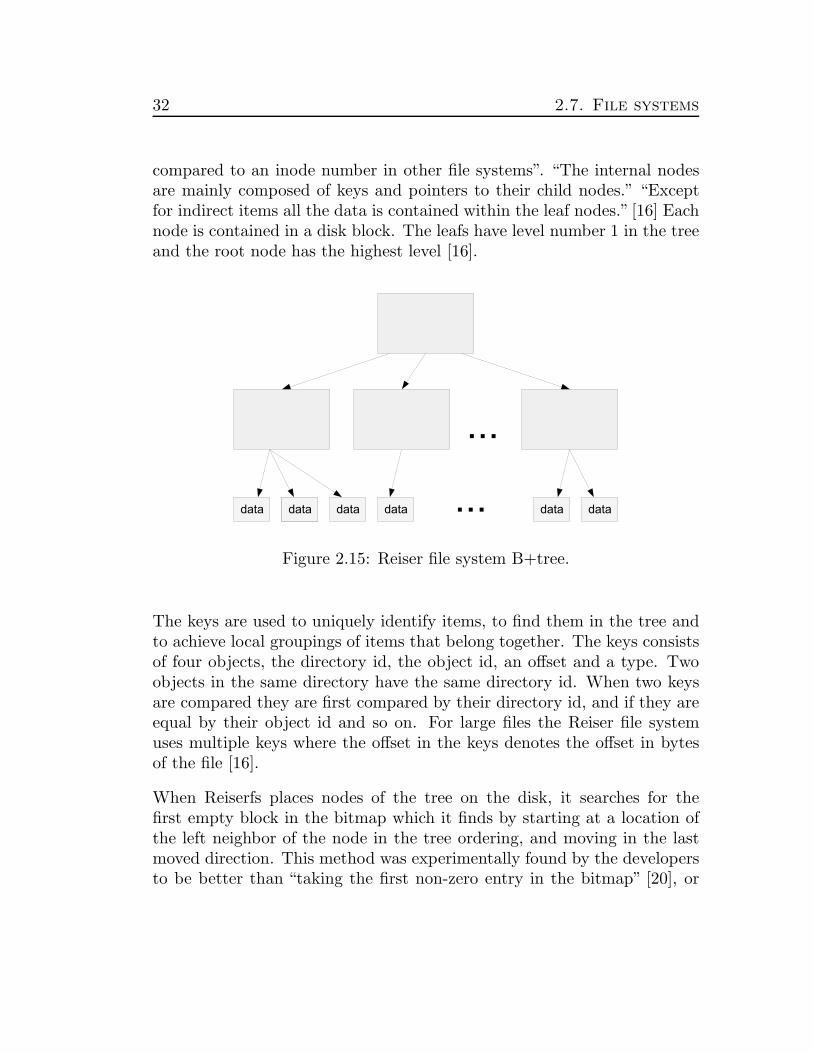
32 2.7. File systems
compared to an inode number in other file systems”. “The internal nodesare mainly composed of keys and pointers to their child nodes.” “Exceptfor indirect items all the data is contained within the leaf nodes.” [16] Eachnode is contained in a disk block. The leafs have level number 1 in the treeand the root node has the highest level [16].
Figure 2.15: Reiser file system B+tree.
The keys are used to uniquely identify items, to find them in the tree andto achieve local groupings of items that belong together. The keys consistsof four objects, the directory id, the object id, an offset and a type. Twoobjects in the same directory have the same directory id. When two keysare compared they are first compared by their directory id, and if they areequal by their object id and so on. For large files the Reiser file systemuses multiple keys where the offset in the keys denotes the offset in bytesof the file [16].
When Reiserfs places nodes of the tree on the disk, it searches for thefirst empty block in the bitmap which it finds by starting at a location ofthe left neighbor of the node in the tree ordering, and moving in the lastmoved direction. This method was experimentally found by the developersto be better than “taking the first non-zero entry in the bitmap” [20], or

Theoretical background 33
“taking the entry after the last one that was assigned in the direction lastmoved” [20], or “starting at the left neighbor and moving in the directionof the right neighbor” [20].
2.7.4 XFS
The XFS file system is a journaled file system. The XFS file system usesB+trees for almost all file system data structures [21].
“XFS is modularized into several parts”[21]. The space manager is a centraland important module which manages the file system free space, the allo-cation of inodes, and the allocation of space within individual files. “TheI/O manager is responsible for satisfying file I/O requests” [21]. “The direc-tory manager implements the XFS file system name space.” [21] The buffercache is used by all these parts to cache contents of frequently accessedblocks in memory for efficiency reasons. The transaction manager is usedby other pieces of the file system so all metadata updates can be atomic.[21].
The XFS partition is split into a number of equally sized chunks calledAG, Allocation Groups. “Each AG has the following characteristics:” [17]“A super block describing overall filesystem info” [17] , “free space man-agement” [17] and “inode allocation and tracking” [17]. The disk layoutstructure of an Allocation Group are shown in figure 2.16. The superblockin the the first Allocation Group is the primary and is used by the filesys-tem. All other superblocks are spare and are only used by xfs repair. Thefirst AG maintains global information about free space across the filesystemand total number of inodes. “Having multiple AGs allows XFS to handlemost operations in parallel” [17].

34 2.7. File systems
Figure 2.16: XFS AG layout.
The superblock contains information about the filesystem, the block size,total number of blocks available, the first block number for the journalinglog, the root inode number in the inode B+tree, the number of levels in theinode B+tree, the AG relative inode number most recently allocated, thesize of each AG in blocks, the number of AGs in the filesystem, the numberof blocks for the journaling log, the underlying disk sector size, the inodesize in bytes, number of inodes per block, name for the filesystem, etc [17].

Theoretical background 35
XFS uses two B+trees to manage free space. One B+tree tracks free spaceby block number and the second B+tree by the size of the free space block.“This scheme allows XFS to quickly find free space near a given block orof a given size.” [17] “The second sector in an AG contains the informationabout the two free space B+trees” [17].
Inodes are allocated in chunks where each chunk contains 64 inodes. AB+tree is used to track the inode chunks of inodes as they are allocatedand freed. The inodes contain almost the same information as in the ext3filesystem. XFS uses extents where the extents specify where the file’s ac-tual data is located within the filesystem. “Extents can have 2 formats”[17]:for small files the“extent data is fully contained within the inode which con-tains an array of extents to the filesystem blocks for the file” [17], for largerfiles the “extent data is contained in the leaves of a B+tree” [17] where the“inode contains the root node of the tree” [17], see figure 2.17 [17].
Figure 2.17: XFS file data structure.

36 2.7. File systems
“The data fork contains the directory’s entries and associated data”[17] andthe format of the entries can be one of 3 formats. For small directorys withfew files the“directory entries are fully contained within the inode”[17]. Formedium size directorys the “actual directory entries are located in anotherfilesystem block” [17] and “the inode contains an array of extents to thesefilesystem blocks” [17]. For large directorys with many files the “directoryentries are contained in the leaves of a B+tree” [17]. “The inode containsthe root node of the tree” [17]. The number of directory entries that canbe stored in an inode depends on the inode size, the number of entries, thelength of the entry names and extended attribute data [17].
In the XFS filesystem the journaling is implemented to journal all meta-data. First XFS writes the updated metadata to an in-core log buffer andthen asynchronously writes the log buffers to the on-disk log [21].

Theoretical background 37
2.7.5 JFS
The journaled file system, JFS, was developed by IBM for the IBM AIXUnix and later ported to Linux [18].
A JFS filesystem is built on top of a partition. The partition can be aphysical partition or a logical volume. The partition is divided in a numberof blocks where each block has the size blocksize. “The partition blocksize defines the smallest unit of I/O” [18]. There is one aggregate in thepartition and it is wholly contained within the partition. “A fileset containsfiles and directories.” [18] A fileset forms an independently mountable sub-tree. “There may be multiple filesets per aggregate” [18], see figures 2.18and 2.19. [18, 22]
Figure 2.18: JFS aggregate with two filesets.
A fileset has a Fileset Inode Table and a Fileset Inode Allocation Map.The Inode Table describes the fileset-wide control structures. The FilesetAllocation Map contains allocation state information on the fileset inodesas well as their on-disk location. The first four, 0–3, inodes in the filesetare used for “additional fileset information that would not fit in the FilesetAllocation Map Inode in the Aggregate Inode Table” [22], root directory

38 2.7. File systems
inode for the fileset, inode for the Access Control List file. “Fileset inodesstarting with four are used by ordinary fileset objects, user files, directories,and symbolic links” [22].
Figure 2.19: A JFS fileset.
The Aggregate superblock maintains information about the entire file sys-tem and includes the following fields: size of the file system, number ofdata blocks in the file system, a flag indicating the state of the file system,allocation group sizes. The secondary superblock is used if the primarysuperblock is corrupted [22].
The Aggregate inode table contains inodes describing the aggregate-widecontrol structures. The secondary Aggregate Inode Table contains repli-cated inodes from the inode table. The inodes in the inode table are criticalfor finding file system information therefore are they duplicated. The Ag-gregate inodes are used for describing the aggregate disk blocks comprisingthe Aggregate Inode Map, describing the Block Allocation Map, describingthe journal log, describing bad blocks, and there is one inode per fileset [22].
The Aggregate Inode Allocation Map contains allocation state informationon the Aggregate inodes as well as their on-disk location. The secondaryAggregate Inode Allocation Map describes the Secondary Aggregate InodeTable [22].
The Block Allocation Map describes the control structures for allocatingand freeing aggregate disk blocks within the aggregate. It is used to trackthe freed and allocated disk blocks for an entire aggregate [22].
JFS allocates inodes dynamically in contiguous chunks of 32 inodes in ainode extent. This allows inode disk blocks to be placed at any disk ad-

Theoretical background 39
dress, which decouples the inode number from the location. It eliminatesthe static allocation of inodes when creating the filesystem. “File allocationfor large files can consume multiple allocation groups and still be contigu-ous” [22]. “With static allocation the geometry of the file system implicitlydescribes the layout of inodes on disk; with dynamic allocation separatemapping structures are required.” [22] The Inode Allocation Map provideswith the function of finding inodes given the inode number. “The Inode Al-location Map is a dynamic array of Inode Allocation Groups (IAGS).” [22]The mapping structures are critical to the JFS integrity [22].
For directories two different directory organizations are provided. The firstis used for small directories, up to 8 entries, and stores the directory con-tents within the directory’s inode (except . and .. which are stored inseparate areas of the inode). This eliminates the need for separate blockI/O and separate block storage. “The second organization is used for largerdirectories and represents each directory as a B+tree keyed on name” [18].
Allocation groups divide the space in an aggregate into chunks where al-location policies try to cluster disk blocks and disk inodes for related datato achieve good locality. Files are often read and written sequentially, andthe files in a directory are often accessed together [22].
“A file is represented by an inode containing the root of a B+tree whichdescribes the extents containing user data.” [22] The B+tree is indexed bythe offset of the extents. “A file is allocated in sequences of extents.” [22]An Extent is a variable length sequence of contiguous aggregate blocksallocated to a JFS object as a unit. The extents are defined by two values,its length, measured in units of aggregate block size, and its address (theaddress to the first block of the extent). The extents are indexed in aB+tree [23, 22].
“JFS uses a transaction-based logging technique to implement recoverabil-ity.” [23] JFS journals the file system structure to ensure that it is alwaysconsistent. “User data is not guaranteed to be fully updated if a systemcrash has occurred” [23]. When the inode information is updated for someinodes the inode information is written to the inode extent buffer. Thenthe record is written. “After the commit record has actually been written

40 2.8. I/O Scheduling Algorithms
(I/O complete), the block map and inode map are updated as needed, andthe tlck’ed meta-data pages are marked ’homeok’ ” [23].
2.8 I/O Scheduling Algorithms
In Linux there are 4 algorithms for handling disk I/O requests, the noopelevator, the complete fairness queueing elevator, the deadline elevator andthe anticipatory elevator. The heuristics is reminiscent of the algorithmused by elevators when dealing with request coming from different floorsto go up or down. “The elevator moves in one direction and when it hasreached the last booked floor the elevator changes direction and starts mov-ing in the other direction” [15].
In the Linux 2.6 kernel up to 2.6.17, including the 2.6.8 used in our tests,the anticipatory elevator is the default algorithm. In 2.6.18 the kerneldevelopers changed algorithm to the complete fairness queueing elevator asthe default algorithm [15, 24].
The Noop elevator is the simplest algorithm of the four algorithms. Thereis no ordered queue and new requests are added either at the end or at thefront of the dispatch queue. “The next request to be served is always thefirst in the dispatch queue” [15].
The Deadline elevator algorithm uses four queues and a dispatch queue.Two queues are sorted queues for read and write requests ordered accordingto their initial sector number. Two queues are deadline queues includingthe same read and write requests sorted according to their deadlines. Theexpire time for read requests is 500 milliseconds and for write requests 5seconds. Read requests are privileged over write requests. The deadlineensures that the scheduler looks at a request if it has been waiting a longtime [15].
“When the elevator replenishes the dispatch queue it determines the datadirection of the next request and if there are both read and write requeststo be dispatched, the elevator chooses the read direction, unless the write

Theoretical background 41
direction has been discarded too many times” [15].
The elevator also checks the deadline queue relative to the chosen direction.If a request in the queue is elapsed, the elevator moves that request to thetail of the dispatch queue. It also moves a batch of requests taken from thesorted queue starting from the request following the expired one [15].
If there are no expired requests the elevator dispatches a batch of requestsstarting with the request following the last one taken from the sorted queue.When the tail of the sorted queue is reached the search starts again fromthe top [15].
The anticipatory elevator uses a dispatch queue, two deadline queues andtwo sorted queues. The algorithm is an evolution of the Deadline elevator.The two sorted queues are one for read requests and one for write requests.The two deadline queues, one for read requests and one for write requests,are sorted according to their “deadlines”. The request are the same as inthe two sorted queues [15].
Figure 2.20: The anticipatory elevator.
The deadline queues are implemented to avoid request starvation, whichoccurs when the elevator policy for a very long time ignores a request be-

42 2.8. I/O Scheduling Algorithms
cause it handle other requests that are closer to the last served one. Arequest deadline is an expire timer that starts when the request is queued.The default expire time for read requests is 125 milliseconds and for writerequests is 250 milliseconds. The I/O scheduler keeps scanning the twosorted queues, alternating between read and write request but giving pref-erence to the read ones and moves the requests to the dispatch queue. Thescanning is sequential, unless a request expires. The scheduler looks atthe deadline queues and checks if there are any requests to expire, then ithandles them and moves them to the dispatch queue, see figure 2.20.
If a request behind another one is less than half the seek distance of therequest after the current position the algorithm chooses that one instead.This forces a backward seek of the disk head [15].
The anticipatory elevator saves statistics about the patterns of I/O oper-ations. The elevator tries to anticipate requests based on the statistics.Right after dispatching a read request that triggered by some process, theanticipatory elevator checks if the next request in the sorted queue comesfrom the same process. If not the elevator looks at the statistics aboutthe process and decides if its likely that the process will issue another readrequest soon, then it stalls for a short period of time [15].
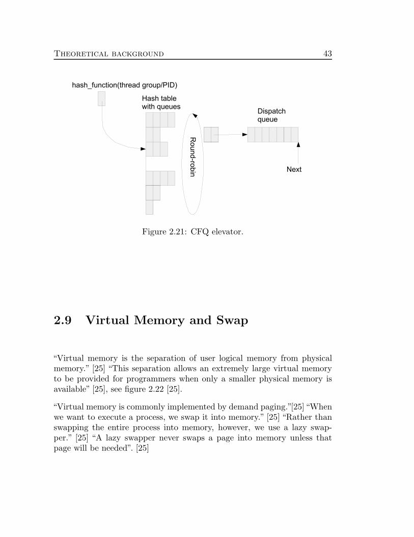
The CFQ, complete fairness queueing, elevator uses a dispatch queue anda hash table with queues. The default number of queues in the hash tableis 64. The hash function converts the thread group identifier of the currentprocess into the index of a queue. The thread group identifier is usuallycorresponding to the PID, Process ID. The elevator scans the I/O inputqueues in a round-robin fashion and refills the tail of the dispatch queuewith a batch of requests [15].
Theoretical background 43
Figure 2.21: CFQ elevator.
2.9 Virtual Memory and Swap
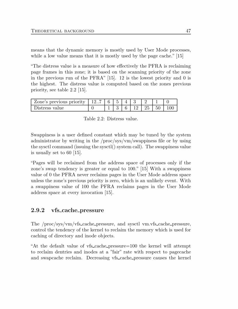
“Virtual memory is the separation of user logical memory from physicalmemory.” [25] “This separation allows an extremely large virtual memoryto be provided for programmers when only a smaller physical memory isavailable” [25], see figure 2.22 [25].
“Virtual memory is commonly implemented by demand paging.”[25] “Whenwe want to execute a process, we swap it into memory.” [25] “Rather thanswapping the entire process into memory, however, we use a lazy swap-per.” [25] “A lazy swapper never swaps a page into memory unless thatpage will be needed”. [25]

44 2.9. Virtual Memory and Swap
Figure 2.22: Virtual memory.
The virtual memory is mapped to physical memory and to swap space(usually a hard disk). When a process is started parts of the program, orthe whole program, is loaded into the physical memory. When we startexecuting a process the operating system sets the instruction pointer tothe first instruction of the process. If that page is not in physical memorya page fault occurs and the page is brought into memory. “After thispage is brought into memory, the process continues to execute, faulting asnecessary until every page that it needs is in memory.” [25] “In this way,we are able to execute a process, even though portions of it are not (yet) inmemory.” [25] When a process tries to allocate more memory it is given thememory if there is enough free physical memory. If there is no free pageframe the OS uses a page-replacement algorithm to select a victim page. Ifthe victim page has been changed it is first written to swap space before itis reused. If a process accesses a swapped-out page a page fault occurs andthe page is swapped in. When swapping in a page it might be neccessaryto first swap out another page [25].
Virtual memory in Linux is implemented by demand paging. It uses thePFRA, Page Frame Reclaiming Algorithm. The main goal of the algo-rithm is to pick up page frames and make them free. PFRA handles page
Theoretical background 45
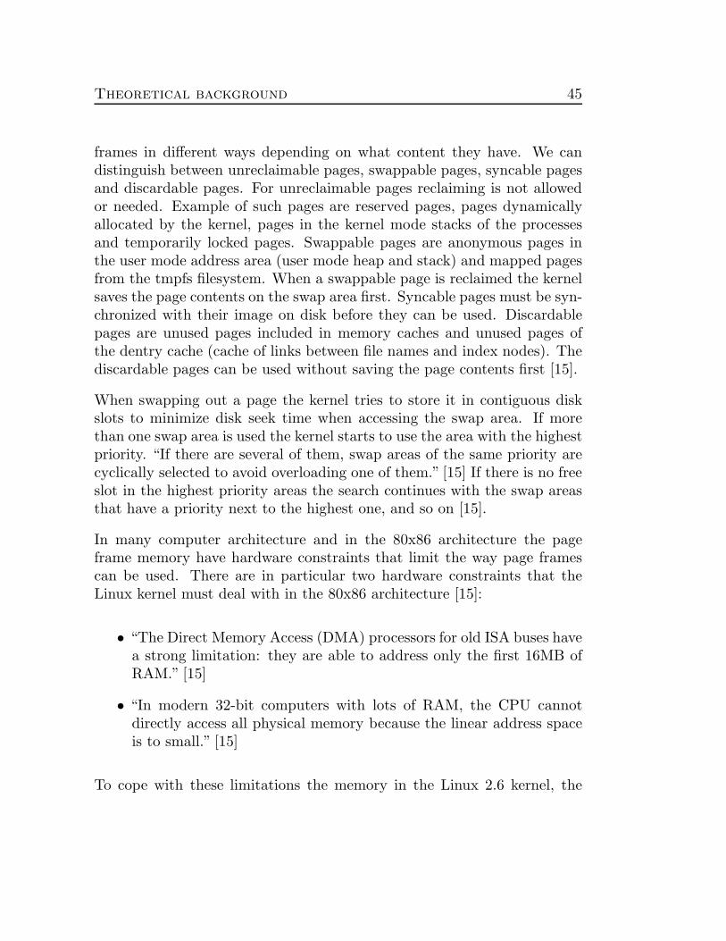
frames in different ways depending on what content they have. We candistinguish between unreclaimable pages, swappable pages, syncable pagesand discardable pages. For unreclaimable pages reclaiming is not allowedor needed. Example of such pages are reserved pages, pages dynamicallyallocated by the kernel, pages in the kernel mode stacks of the processesand temporarily locked pages. Swappable pages are anonymous pages inthe user mode address area (user mode heap and stack) and mapped pagesfrom the tmpfs filesystem. When a swappable page is reclaimed the kernelsaves the page contents on the swap area first. Syncable pages must be syn-chronized with their image on disk before they can be used. Discardablepages are unused pages included in memory caches and unused pages ofthe dentry cache (cache of links between file names and index nodes). Thediscardable pages can be used without saving the page contents first [15].
When swapping out a page the kernel tries to store it in contiguous diskslots to minimize disk seek time when accessing the swap area. If morethan one swap area is used the kernel starts to use the area with the highestpriority. “If there are several of them, swap areas of the same priority arecyclically selected to avoid overloading one of them.” [15] If there is no freeslot in the highest priority areas the search continues with the swap areasthat have a priority next to the highest one, and so on [15].
In many computer architecture and in the 80x86 architecture the pageframe memory have hardware constraints that limit the way page framescan be used. There are in particular two hardware constraints that theLinux kernel must deal with in the 80x86 architecture [15]:
• “The Direct Memory Access (DMA) processors for old ISA buses havea strong limitation: they are able to address only the first 16MB ofRAM.” [15]
• “In modern 32-bit computers with lots of RAM, the CPU cannotdirectly access all physical memory because the linear address spaceis to small.” [15]
To cope with these limitations the memory in the Linux 2.6 kernel, the
46 2.9. Virtual Memory and Swap
physical memory is partitioned into three zones. In the 80x86 architecturethe zones are [15]:
ZONE DMA Contains frames of memory below 16MB
ZONE NORMAL Contains frames of memory from 16MB to 896MB
ZONE HIGHMEM Contains frames of memory from and above 896MB
In the Linux kernel all memory pages belonging to the User Mode addressspace and to the page cache are grouped into two lists, the active list thattends to include the pages that have been accessed recently and the inactivelist that tends to include the pages that have not been accessed for sometime. The function refill inactive zone() moves pages from the active list tothe inactive list. The function must not be too aggressive and move a largenumber of pages from the active list to the inactive list. In that case thesystem performance will be hit.”On the other hand, if the function is toolazy, the inactive list will not be replenished with a large enough number ofunused pages” [15]. In that case the PFRA will fail in reclaiming memory.
In the kernel there are a group of kernel threads called pdflush. The pdflushsystematically scan the page cache looking for dirty pages, pages that hasbeen changed, to flush [15].
2.9.1 Swappiness
The refill inactive zone() function uses swap tendency which regulates itsbehaviour. “The swap tendency value is computed by the function as fol-lows” [15]:
“swap tendency = mapped ratio / 2 + distress + swappiness” [15]
“The mapped ratio value is the percentage of pages in all memory zonesthat belong to User Mode address spaces (sc->nr mapped) with respect tothe total number of allocatable page frames. A high value of mapped ratio
Theoretical background 47
means that the dynamic memory is mostly used by User Mode processes,while a low value means that it is mostly used by the page cache.” [15]
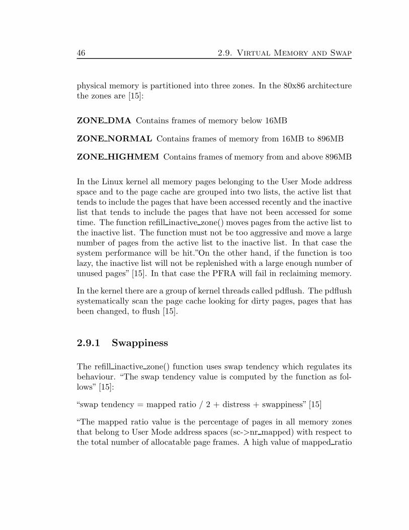
“The distress value is a measure of how effectively the PFRA is reclaimingpage frames in this zone; it is based on the scanning priority of the zonein the previous run of the PFRA” [15]. 12 is the lowest priority and 0 isthe highest. The distress value is computed based on the zones previouspriority, see table 2.2 [15].
Zone’s previous priority 12..7 6 5 4 3 2 1 0Distress value 0 1 3 6 12 25 50 100
Table 2.2: Distress value.
Swappiness is a user defined constant which may be tuned by the systemadministrator by writing in the /proc/sys/vm/swappiness file or by usingthe sysctl command (issuing the sysctl() system call). The swappiness valueis usually set to 60 [15].
“Pages will be reclaimed from the address space of processes only if thezone’s swap tendency is greater or equal to 100.” [15] With a swappinessvalue of 0 the PFRA never reclaims pages in the User Mode address spaceunless the zone’s previous priority is zero, which is an unlikely event. Witha swappiness value of 100 the PFRA reclaims pages in the User Modeaddress space at every invocation [15].
2.9.2 vfs cache pressure
The /proc/sys/vm/vfs cache pressure, and sysctl vm.vfs cache pressure,control the tendency of the kernel to reclaim the memory which is used forcaching of directory and inode objects.
“At the default value of vfs cache pressure=100 the kernel will attemptto reclaim dentries and inodes at a ”fair” rate with respect to pagecacheand swapcache reclaim. Decreasing vfs cache pressure causes the kernel

48 2.9. Virtual Memory and Swap
to prefer to retain dentry and inode caches. Increasing vfs cache pressurebeyond 100 causes the kernel to prefer to reclaim dentries and inodes.” [26]
2.9.3 dirty ratio and dirty background ratio
With these parameters it is possible to control the syncing of dirty data.
The /proc/sys/vm/dirty ratio, and the sysctl vm.dirty ratio, “contains, asa percentage of total system memory, the number of pages at which aprocess which is generating disk writes will itself start writing out dirtydata” [26].
The /proc/sys/vm/dirty background ratio, and the sysctl vm.dirty background ratio,“contains, as a percentage of total system memory, the number of pages atwhich the pdflush background writeback daemon will start writing out dirtydata” [26].
2.9.4 min free kbytes
The /proc/sys/vm/min free kbytes, and sysctl vm.min free kbytes, is usedto force the Linux VM to keep a minimum number of kilobytes RAM free.“The VM uses this number to compute a pages min value for each lowmemzone in the system. Each lowmem zone gets a number of reserved free pagesbased proportionally on its size.” [27]
2.9.5 page-cluster
“The Linux VM subsystem avoids excessive disk seeks by reading multiplepages on a page fault. The number of pages it reads is dependent on theamount of memory in your machine.” [27]
“The number of pages the kernel reads in at once is equal to 2page−cluster.Values above 25 don’t make much sense for swap because we only cluster

Theoretical background 49
swap data in 32-page groups.” [27]
The value is defined bye the /proc/sys/vm/page-cluster, and the sysctlvm.page-cluster. [27]
2.9.6 dirty writeback centisecs
The /proc/sys/vm/dirty writeback centisecs, and sysctl vm.dirty writeback centisecs,controls how often the pdflush writeback daemon will wake up and writeold data out to disk. “This tunable expresses the interval between thosewakeups, in 100’ths of a second.” [26].

50 2.9. Virtual Memory and Swap

Chapter 3
Realization
The goal of this thesis is to examine if it is possible to increase the sizeof the running simulations with 50% more NEs on existing hardware withoperating system environment tuning. To see if it was possible we neededto run test runs and measure the test runs by comparing them with areference test.
We decided to test one parameter at a time and see which of them madeimprovements.
3.1 The test environment
The test environment consisted of 2 computers, one for the NETSim sim-ulations, running Suse Linux 9.2, and one for the load generator, runningSolaris 9, and a local network between them. The NETSim computer wasan HP DL145 G1 with two single core AMD Opteron 2.4 GHz CPUs, 8GBRAM and two Ultra SCSI disks. Unfortunately they were not the onlycomputers on the local network. However the network load was low and
51

52 3.1. The test environment
should therefore not have affected on our test runs. We wanted to testonly the simulations, not the combination of simulation and load genera-tor, therefore the need of two computers. We wanted to be independent ofexternal servers, so we used local user accounts. The test environment is astandard test environment for NETSim.
The computer running NETSim was reinstalled before the test runs with astandard installation of Suse 9.2. The installation of Linux was automatedwith autoyast/jumpstart and the installation of NETSim was automatedwith shell scripts which give that the NETSim computer’s software andconfiguration always was exactly the same for all test runs.
Our test nets consisted of 100 NEs, Network Elements, where 98 NEs wasRBS’s, one RNC and one RXI.
To find out where the limit for the computer running the simulations waswe ran simulations with 8, 9, 10 and 11 nets. During these test runs andall the rest of the test runs we supervised the load generator by measuringthe alarm rate, PM, AVC, nesync and SWUG with the program moodss,see figure 3.1. Moodss is a opensource software which can be found athttp://moodss.sourceforge.net/ . Moodss is frequently used at NETSim atEricsson.

Realization 53
Figure 3.1: Moodss supervising the load generator.

54 3.1. The test environment
We also supervised the two computers load, memory usage and swap usagewith moodss, see figure 3.2.
Figure 3.2: Moodss supervising a computer running NETSim.
Apart from monitoring the load, memory usage and swap usage with moodsswe did run extra tests to study the processor usage and network usage.
The maximum response time is 2 minutes for all of the above. This 2minute limit is defined by OSS. At 11 nets the time limit was exceededwith some errors as a consequence. Exceeding the time limit is an error.The conclusion was that 10 nets with 1000 NEs was the upper limit for thiscomputer without optiminations applied.
The test run with 10 nets then became our reference run. All parametershad their default values in this test. Thus the goal of this thesis is toexamine if it is possible to run NETSim with 15 nets on the computer we
Realization 55
used for the NETSim tests.
When changing a parameter on the computer running the simulations thecomputer was first reinstalled. The only exception was for the virtualmemory parameters which could be changed without reinstalling or rebootthe computer.
All NETSim files and load generator temporary files were located on thesame local file system during all our tests. Load generator temporary filesis the part of the load generator that resides on the NETSim computer.
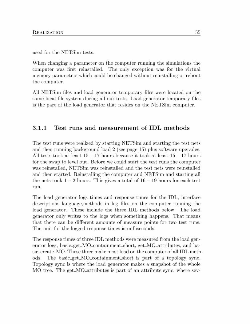
3.1.1 Test runs and measurement of IDL methods
The test runs were realized by starting NETSim and starting the test netsand then running background load 2 (see page 15) plus software upgrades.All tests took at least 15 – 17 hours because it took at least 15 – 17 hoursfor the swap to level out. Before we could start the test runs the computerwas reinstalled, NETSim was reinstalled and the test nets were reinstalledand then started. Reinstalling the computer and NETSim and starting allthe nets took 1 – 2 hours. This gives a total of 16 – 19 hours for each testrun.
The load generator logs times and response times for the IDL, interfacedescriptions language,methods in log files on the computer running theload generator. These include the three IDL methods below. The loadgenerator only writes to the logs when something happens. That meansthat there can be different amounts of measure points for two test runs.The unit for the logged response times is milliseconds.
The response times of three IDL methods were measured from the load gen-erator logs, basic get MO containment short, get MO attributes, and ba-sic create MO. These three make most load on the computer of all IDL meth-ods. The basic get MO containment short is part of a topology sync.Topology sync is where the load generator makes a snapshot of the wholeMO tree. The get MO attributes is part of an attribute sync, where sev-

56 3.1. The test environment
eral MO’s with several IDL methods are synced by the load generator. Thebasic create MO is done as a part of the SWUG where the NEs collect anUpgrade Control File, an XML file, who parse the XML file. The XML filecontains information about the software upgrade such as where to find thesoftware file and how to get it.

Realization 57
Mean value calculations with sliding window
To be able to interpret the test results we did a mean value calculationof the response times by dividing them in two intervals and calculate oneinterval at a time. Without doing that the oscillation of the response timesfor the IDL methods were too fast to see anything and it was impossibleto draw any conclusions.
We divided the two test runs to be compared into intervals, where thenumber of intervals were equal to the number of SWUG cycles. A SWUGcycle is from the start of a SWUG to the start of the next SWUG. Theintervals from the two compared runs where synced with the SWUG cyclesby using the start and end times from the SWUG cycles, see figure 3.3.
Figure 3.3: Mean value calculation of response times.
Each SWUG cycle was divided into equal partial intervals to get an equal
58 3.1. The test environment
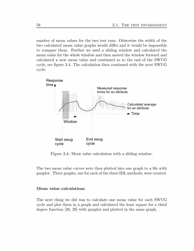
number of mean values for the two test runs. Otherwise the width of thetwo calculated mean value graphs would differ and it would be impossibleto compare them. Further we used a sliding window and calculated themean value for the whole window and then moved the window forward andcalculated a new mean value and continued so to the end of the SWUGcycle, see figure 3.4. The calculation then continued with the next SWUGcycle.
Figure 3.4: Mean value calculation with a sliding window.
The two mean value curves were then plotted into one graph to a file withgnuplot. Three graphs, one for each of the three IDL methods, were created.
Mean value calculations
The next thing we did was to calculate one mean value for each SWUGcycle and plot them in a graph and calculated the least square for a thirddegree function [28, 29] with gnuplot and plotted in the same graph.

Realization 59
f(x) = a1*x*x*x + b1*x*x + c1*x + d1g(x) = a2*x*x*x + b2*x*x + c2*x + d2fit f(x) "file1" via a, b, cfit g(x) "file2" via d, e, h
plot f(x) title "~s" with lines lt 9, g(x) title "~s" with lines lt -1
In separate graphs the mean values were complemented with whisker barswith median, quartile 1 and 3 and min95- and max95- values. 1st and3’d quartile is the median of the lower respectively upper half of the data,where the median of the whole set is not included. Max95 and Min95 isthe greatest respectively smallest value of the data, not included 5% of theoutliners. Outliners are the 5% extremest values.
Figure 3.5: A whisker bar.
The graphs show the deviation for the measured IDL methods in one testrun. See figure 3.6 for an hypothetic example.

60 3.1. The test environment
These two graphs were easier to calculate, took less time to calculate andgave the same result as the first type with sliding window.
Figure 3.6: Mean value calculation with whisker bars and least square fora third degree function.
Times for SWUG’s
SWUG’s are heavy and cause a lot of load on the NEs that are upgradedduring the software upgrade. It is therefore interesting to study the time ittakes to do all SWUG’s. We complemented with studying and comparingthe time it took for one SWUG cycle from start to nesync at the end ofthe SWUG cycle, see figure 3.7.

Realization 61
Figure 3.7: Start and end of a SWUG.
The sample times are discrete values and the start of a SWUG can occurbetween two values and the end of an nesync can occur between two values.To see the time differences the graphs contains the minimum and maximumtimes for a SWUG from start of SWUG to end of nesync, see figure 3.8.

62 3.1. The test environment
Figure 3.8: Maximum and minimum time difference for SWUG’s.
See figure 3.9 for an example of a plot of time difference for a number ofSWUG’s in a hypothetic test run.
Figure 3.9: Time difference for SWUG’s.

Realization 63
Two time difference curves from two test runs were plotted in the samegraph. See figure 3.10 for a hypothetic example.
Figure 3.10: Time difference for SWUG’s for two test runs.
Disk access load
To measure the disk access load, read and write from and to disk, during atest run we ran a test on a Sun Fire T2000 with Solaris 10 and measured alldisk activities with a dtrace script rwsnoop. The hard drives were two SASinterfaced, Serial Attached SCSI, FUJITSU MAY2073RCSUN72G 73.4GBwith an approximate read and write speed at 300 Mbyte/s, Interface SAS(3Gbps) [30]. The result was summarized, in Mbyte, with the followingawk script.
awk ’BEGIN {c = 0} { c = c + $9} END { print c/(1024*1024)}’ datafile
The results are shown in table 3.1 and peak values in figures 3.11 and 3.12.

64 3.1. The test environment
PM/SWUG/ Number of nets MByte data Time (minutes) MByte/sBackground loadBackground load 1 7.1478 8 0.01PM 1 121.353 4 0.5PM 2 241.246 3 1.3SWUG 1 131.953 15 0.1SWUG 1 137.172 15 0.2SWUG 2 272.583 17 0.3
Table 3.1: Disk accesses.
0
1
2
3
4
5
6
7
8
9
10
51800 51900 52000 52100 52200 52300 52400 52500 52600 52700 52800
MB
yte
Time in s
Disk IO for SWUG on 1 net.
Figure 3.11: SWUG with 1 net.
Realization 65
0
2
4
6
8
10
12
58550 58600 58650 58700 58750 58800 58850 58900 58950 59000
MB
yte
Time in s
Disk IO for SWUG on 2 nets.
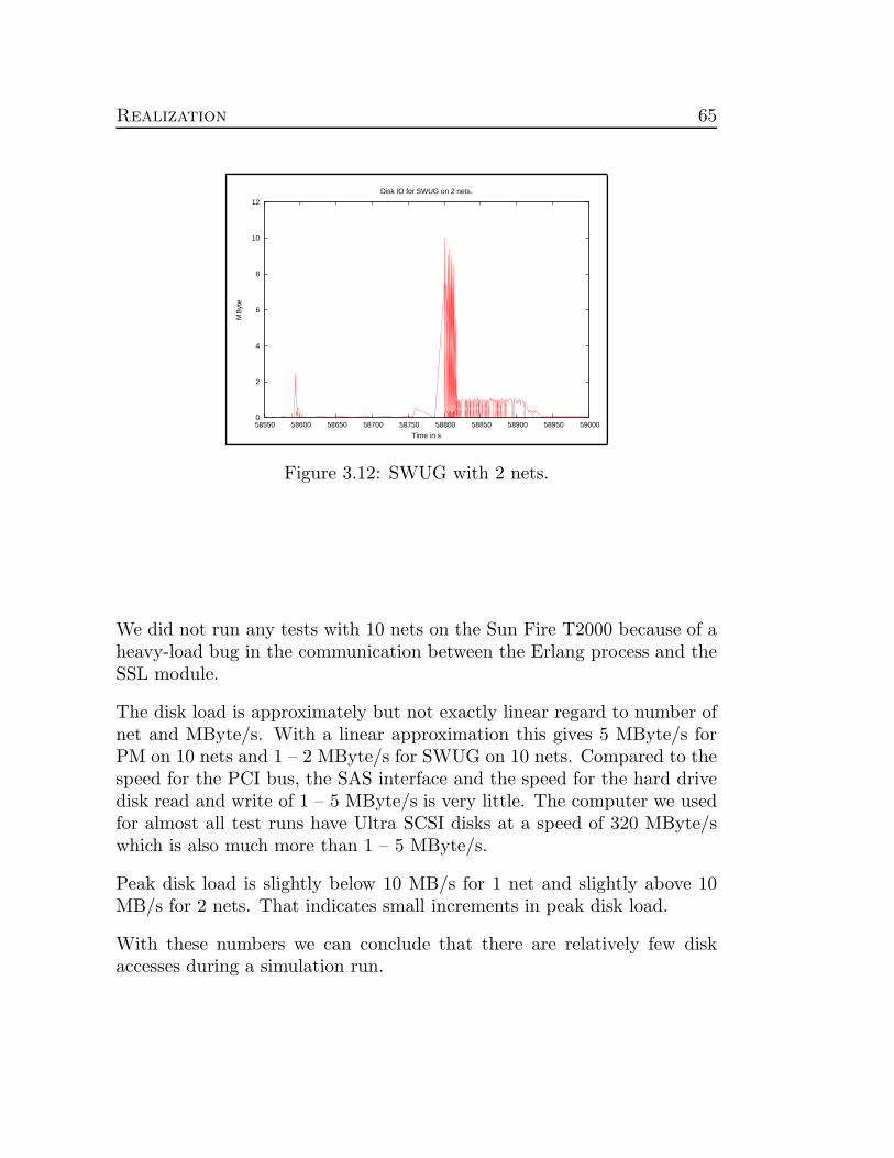
Figure 3.12: SWUG with 2 nets.
We did not run any tests with 10 nets on the Sun Fire T2000 because of aheavy-load bug in the communication between the Erlang process and theSSL module.
The disk load is approximately but not exactly linear regard to number ofnet and MByte/s. With a linear approximation this gives 5 MByte/s forPM on 10 nets and 1 – 2 MByte/s for SWUG on 10 nets. Compared to thespeed for the PCI bus, the SAS interface and the speed for the hard drivedisk read and write of 1 – 5 MByte/s is very little. The computer we usedfor almost all test runs have Ultra SCSI disks at a speed of 320 MByte/swhich is also much more than 1 – 5 MByte/s.
Peak disk load is slightly below 10 MB/s for 1 net and slightly above 10MB/s for 2 nets. That indicates small increments in peak disk load.
With these numbers we can conclude that there are relatively few diskaccesses during a simulation run.

66 3.2. The tests
3.2 The tests
3.2.1 RAID
We choose RAID-0 because we do not need fault tolerance, and just wantimproved I/O performance. We implemented Suses built-in software RAIDon two physical disks with 4 K bytes chunk size. The root- and swap-partitions were not RAID:ed and each lying on one of the two disks 3.13.
Figure 3.13: RAID-0 with two disks.
3.2.2 Crypto Accelerator Card
Because NETSim use Corba over SSL for comunication, heavy crypto cal-culations could be eliminated with a crypto accelerator card. We testedSun Crypto Accelerator 6000 PCI-E Board on a HP ProLiant DL145 G2with two dualcore AMD Opteron model 285 2.6GHz processors runningSuse 9. The crypto accelerator card supports hash functions SHA1 andMD5, block ciphers DES, 3DES and AESSun and RSA/DH public key,with lengths of 512-2,048 bits. Sun Microsystems Inc. does not officiallysupport other platforms than Sun workstations and servers, but supportsSuse 9. We use OpenCryptoki as a bridge between OpenSSL and Suns

Realization 67
device driver. OpenCryptoki is a PKCS#11, Public Key CryptographyStandard, wrapper. OpenCryptoki and OpenSSL are open source, whileSuns device driver is proprietary. With OpenSSL and Suns crypto accelera-tor card, we measure double performance in RSA verifying and signing. Wecould not test NETSim with Suns crypto accelerator card, because Sunsdevice driver did not work faultlessly on the HP platforms.
3.2.3 File systems
The file system used in the reference test was Reiserfs version 3. We testedthe other major file systems in Linux, ext3, XFS and JFS and comparedthem with Reiserfs. For ext3 we did two tests, one with default values andone with index and no update of atime.
In NETSim there are relatively few disk accesses, so changing the file systemshould only have a small impact on the test run.
3.2.4 I/O Scheduling Algorithms
In Linux there are 4 I/O scheduling algorithms. The two most interestingof them are the Anticipatory elevator and the CFQ elevator. They areinteresting because the Anticipatory elevator was the default elevator inthe Linux kernel up to version 2.6.17 and the CFQ elevator is the defaultelevator in the kernel from 2.6.18. Therefore we wanted to test and comparethese two algorithms with each other. Both algorithms were tested with a2.6.8 kernel.
The I/O scheduling algorithm should have little impact on the relativelyfew disk accesses but it should have more effect on the swap usage whenrunning large simulations with large memory usage with much swapping.

68 3.2. The tests
3.2.5 Virtual Memory and Swap
We tested swap on two partitions on two different disks with the samepriority for both swap partitions. This should have some effect on largesimulations with large memory usage especially when the system starts toswap and needs to swap very much. The effect might be less if the NETSimpartition lays on the same disk as one of the partitions. In that case NE diskaccesses might occur at the same time as swap accesses so the read/writehead needs to move a lot over the disk. If that happens it might be betterto have the swapspace on a separate disk.
The virtual memory parameters that we tested was swappiness,vfs cache pressure, dirty ratio, dirty background ratio, min free kbytes, page-cluster, and dirty writeback centisecs.
swappiness
The default value for swappiness is 60. We tested with swappiness 30and 90. It is overall better to swap less especially when there are timerequirements on operations depending on memory and with that dependingon swap. The time limit on operations on NEs in NETSim is 2 minutes.So it should be better to have a lower value on swappiness than a higherone.
vfs cache pressure
The default value for vfs cache pressure is 100. We tested withvfs cache pressure 50 and 150.
With the relatively few disk accesses it should be better to reuse the cachememory used for directories and i-nodes and use the memory for NEs. A

Realization 69
vfs cache pressure value 100 should be better than 50, and 150 might beeven better.
dirty ratio and dirty background ratio
The default value for dirty background ratio is 10 and for vm dirty ratioit is 40.
In a mail to the Linux Kernel Mailing List Linus Torvalds recommends toset the dirty background ratio to 5 and dirty ratio to 10 [31].
Date Fri, 27 Apr 2007 08:18:34 -0700 (PDT)From Linus Torvalds <>Subject Re: [ext3][kernels >= 2.6.20.7 at least] KDE going comatose when FS is under
heavy write load (massive starvation)Digg This
On Fri, 27 Apr 2007, Mike Galbraith wrote:>> As subject states, my GUI is going away for extended periods of time> when my very full and likely highly fragmented (how to find out)> filesystem is under heavy write load. While write is under way, if> amarok (mp3 player) is running, no song change will occur until write is> finished, and the GUI can go _entirely_ comatose for very long periods.> Usually, it will come back to life after write is finished, but> occasionally, a complete GUI restart is necessary.
One thing to try out (and dammit, I should make it the default now in2.6.21) is to just make the dirty limits much lower. We’ve been talkingabout this for ages, I think this might be the right time to do it.
Especially with lots of memory, allowing 40% of that memory to be dirty isjust insane (even if we limit it to "just" 40% of the normal memory zone.That can be gigabytes. And no amount of IO scheduling will make itpleasant to try to handle the situation where that much memory is dirty.
So I do believe that we could probably do something about the IOscheduling _too_:
- break up large write requests (yeah, it will make for worse IOthroughput, but if make it configurable, and especially withcontrollers that don’t have insane overheads per command, thedifference between 128kB requests and 16MB requests is probably notreally even noticeable - SCSI things with large per-command overheadsare just stupid)

70 3.2. The tests
Generating huge requests will automatically mean that they are"unbreakable" from an IO scheduler perspective, so it’s bad for latencyfor other reqeusts once they’ve started.
- maybe be more aggressive about prioritizing reads over writes.
but in the meantime, what happens if you apply this patch?
Actually, you don’t need to apply the patch - just do
echo 5 > /proc/sys/vm/dirty_background_ratioecho 10 > /proc/sys/vm/dirty_ratioand say if it seems to improve things. I think those are much sanerdefaults especially for a desktop system (and probably for most serverstoo, for that matter).
Even 10% of memory dirty can be a whole lot of RAM, but it shouldhopefully be _better_ than the insane default we have now.
Historical note: allowing about half of memory to contain dirty pages mademore sense back in the days when people had 16-64MB of memory, and asingle untar of even fairly small projects would otherwise hit the disk.But memory sizes have grown *much* more quickly than disk speeds (andlatency requirements have gone down, not up), so a default that mayactually have been perfectly fine at some point seems crazy these days..
Linus’’
Therefore we decided to run a test with dirty background ratio = 5 anddirty ratio = 10.
min free kbytes
Our default value for min free kbytes is 282 MBytes RAM. The recom-mended value for NETSim is at least 2% of the total size of RAM in thecomputer. With less than 1–2% min free kbytes the device drivers couldnot always allocate memory.
We ran one test with min free kbytes 158MB which was 2% of RAM in ourcase with our computer. As seen above less than 1–2% min free kbytes isnot good. With a too high value a lot of memory stays unused and the

Realization 71
operating system needs to swap more. Therefore a too high value is notgood.
page-cluster
The default value for page-cluster is 3. We tested page-cluster values of1 and 5. Page-cluster should have little effect on the relatively few diskaccesses but it should have more impact on large simulations with largememory usage and much swapping.
dirty writeback centisecs
The default value for dirty writeback centisecs is 500. We tested witha dirty writeback centisecs value of 1000. The dirty writeback centisecsshould have little effect on the relatively few disk accesses.

72 3.2. The tests

Chapter 4
Results
In this chapter we present the test results of our tests. All response timesbelow are in milliseconds.
4.1 Mean with sliding window
Besides the test runs with different values for the different paramaters werun three reference runs and compared them with each other. The resultswere plotted with mean value calculation with sliding window. Figure 4.1shows the IDL method get MO attributes for two reference runs, ref 1 andref 2. We compared the IDL methods for two test runs at a time becausethat was what our program was designed for.
73

74 4.1. Mean with sliding window
0
2000
4000
6000
8000
10000
12000
0 100 200 300 400 500 600
Res
pons
etim
e
Value
Attributes
Original 1Original 2
Figure 4.1: Comparing get MO attributes for two reference runs.
Figure 4.2 shows IDL method get MO attributes for reference run 2 andtest run with 2 separate swap partitions.
0
2000
4000
6000
8000
10000
12000
0 100 200 300 400 500 600
Res
pons
etim
e
Value
Attributes
Swap on 1 partitionSwap on 2 partitions
Figure 4.2: Comparing get MO attributes for reference run 2 and a swaprun.

Results 75
Figure 4.3 shows the IDL method basic create MO for two reference runs,ref 1 and ref 2.
0
5000
10000
15000
20000
25000
30000
0 100 200 300 400 500 600
Res
pons
etim
e
Value
Create_MO
Original 1Original 2
Figure 4.3: Comparing basic create MO for two reference runs.

76 4.1. Mean with sliding window
Figure 4.4 shows the IDL method basic create MO for reference run 2 andtest run with 2 separate swap partitions.
0
5000
10000
15000
20000
25000
30000
0 100 200 300 400 500 600
Res
pons
etim
e
Value
Create_MO
Swap on 1 partitionSwap on 2 partitions
Figure 4.4: Comparing basic create MO for reference run 2 and a swaprun.

Results 77
Figure 4.5 shows the IDL method basic get MO containment short for tworeference runs, ref 1 and ref 2.
0
500
1000
1500
2000
0 100 200 300 400 500 600
Res
pons
etim
e
Value
Get_MO
Original 1Original 2
Figure 4.5: Comparing basic get MO containment short for two referenceruns.

78 4.1. Mean with sliding window
Figure 4.6 shows the IDL method basic get MO containment short for ref-erence run 2 and test run with 2 separate swap partitions.
0
500
1000
1500
2000
0 100 200 300 400 500 600
Res
pons
etim
e
Value
Get_MO
Swap on 1 partitionSwap on 2 partitions
Figure 4.6: Comparing basic get MO containment short for reference run2 and a swap run.

Results 79
4.2 Mean with whisker bars
We plotted graphs with mean values, one for each SWUG, and combinedthem with least square for a second degree function and whisker bars.Figure 4.7 shows the IDL method get MO attributes for two reference runs,ref 1 and ref 2.
0
10000
20000
30000
40000
50000
60000
0 10000 20000 30000 40000 50000 60000 70000
Res
pons
etim
e
Time
Attributes Whiskerbars Combined
Original 1Original 2
Figure 4.7: Comparing get MO attributes for two reference runs withwhisker bars.

80 4.2. Mean with whisker bars
Figure 4.8 shows the IDL method basic create MO for two reference runs,ref 1 and ref 2 with whisker bars.
0
10000
20000
30000
40000
50000
60000
70000
0 10000 20000 30000 40000 50000 60000 70000
Res
pons
etim
e
Time
Create_MO Whiskerbars Combined
Original 1Original 2
Figure 4.8: Comparing basic create MO for two reference runs with whiskerbars.

Results 81
Figure 4.9 shows the IDL method basic get MO containment short for tworeference runs, ref 1 and ref 2 with whisker bars.
0
1000
2000
3000
4000
5000
6000
7000
0 10000 20000 30000 40000 50000 60000 70000
Res
pons
etim
e
Time
Get_MO Whiskerbars Combined
Original 1Original 2
Figure 4.9: Comparing basic get MO containment short for two referenceruns with whisker bars.

82 4.2. Mean with whisker bars
Figure 4.10 shows the IDL method get MO attributes for reference run 2and test run with 2 separate swap partitions with whisker bars.
0
10000
20000
30000
40000
50000
60000
0 10000 20000 30000 40000 50000 60000 70000
Res
pons
etim
e
Time
Attributes Whiskerbars Combined
1 swap partition2 swap partitions
Figure 4.10: Comparing get MO attributes for reference run 2 and a swaprun with whisker bars.
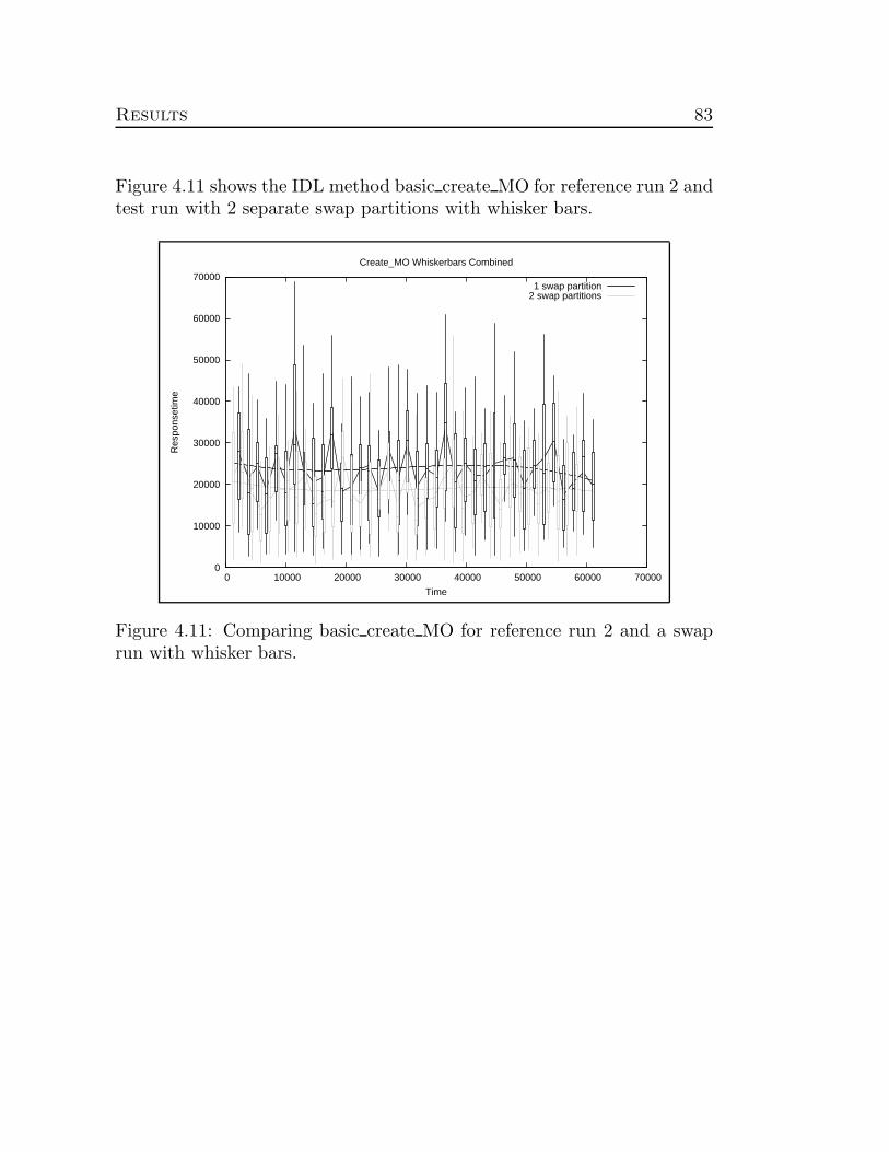
Results 83
Figure 4.11 shows the IDL method basic create MO for reference run 2 andtest run with 2 separate swap partitions with whisker bars.
0
10000
20000
30000
40000
50000
60000
70000
0 10000 20000 30000 40000 50000 60000 70000
Res
pons
etim
e
Time
Create_MO Whiskerbars Combined
1 swap partition2 swap partitions
Figure 4.11: Comparing basic create MO for reference run 2 and a swaprun with whisker bars.

84 4.3. Swug-times
Figure 4.12 shows the IDL method basic get MO containment short forreference run 2 and test run with 2 separate swap partitions with whiskerbars.
0
1000
2000
3000
4000
5000
6000
7000
0 10000 20000 30000 40000 50000 60000 70000
Res
pons
etim
e
Time
Get_MO Whiskerbars Combined
1 swap partition2 swap partitions
Figure 4.12: Comparing basic get MO containment short for reference run2 and a swap run with whisker bars.
4.3 Swug-times
We plotted time differences for SWUG cycles from start of SWUG to endof nesync. Figure 4.13 shows the difference times for SWUGs for referencerun 1 and 2.

Results 85
0
500
1000
1500
2000
0 5 10 15 20 25 30
Tim
e
Nr of Swug
Swugtimes-diff
Original 1 MaxOriginal 1 Min
Original 2 MaxOriginal 2 Min
Figure 4.13: Time difference for SWUGs for two reference runs.
Figure 4.14 shows the difference times for SWUGs for reference run 2 andfor a test run with swap on 2 separate partitions.
0
500
1000
1500
2000
0 5 10 15 20 25 30
Tim
e
Nr of Swug
Swugtimes-diff
1 swap partition Max1 swap partition Min
2 swap partitions Max2 swap partitions Min
Figure 4.14: Time difference for SWUGs for two test runs.

86 4.4. Memory usage
4.4 Memory usage
When we run a simulation with 10 nets on a computer with 8 GB RAMthe memory usage increased during the simulation run and the computerstarted to swap after 10–12 hours, see figure 4.15.
Figure 4.15: Memory and swap usage.
The memory and swap used increased and after 15–17 hours the swapreached around 5GB then the swap started to level out, see figure 4.16.
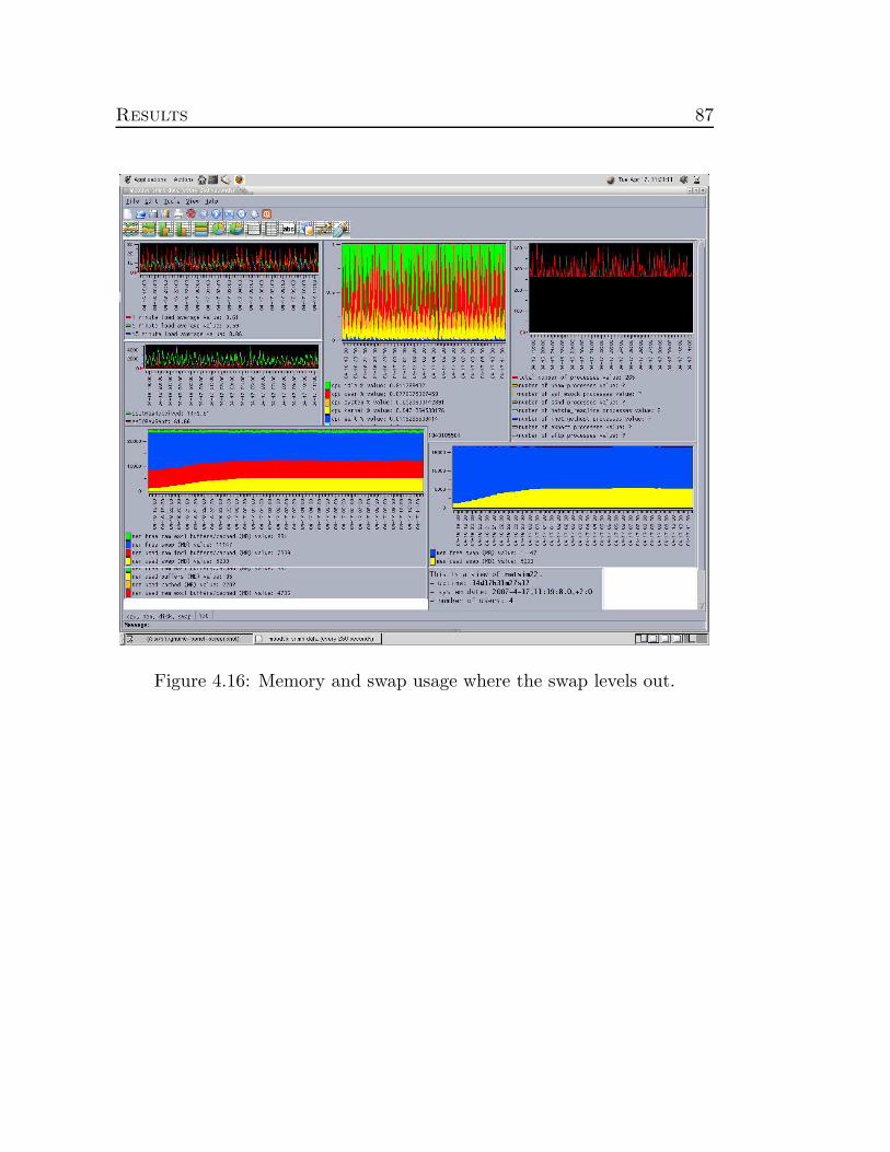
Results 87
Figure 4.16: Memory and swap usage where the swap levels out.

88 4.4. Memory usage
Figure 4.17 shows CPU and memory usage for 8 nets on a computer with8GB RAM. The maximum memory used was 4521 MB RAM. This run waslittle to short for the swap to level out.
Figure 4.17: CPU, memory and swap usage for 8 nets.
Figure 4.18 shows CPU and memory usage for 10 nets on a computer with8GB RAM. The maximum memory used was 4736 MB RAM and usedswap was 5239 MB.

Results 89
Figure 4.18: CPU, memory and swap usage for 10 nets.
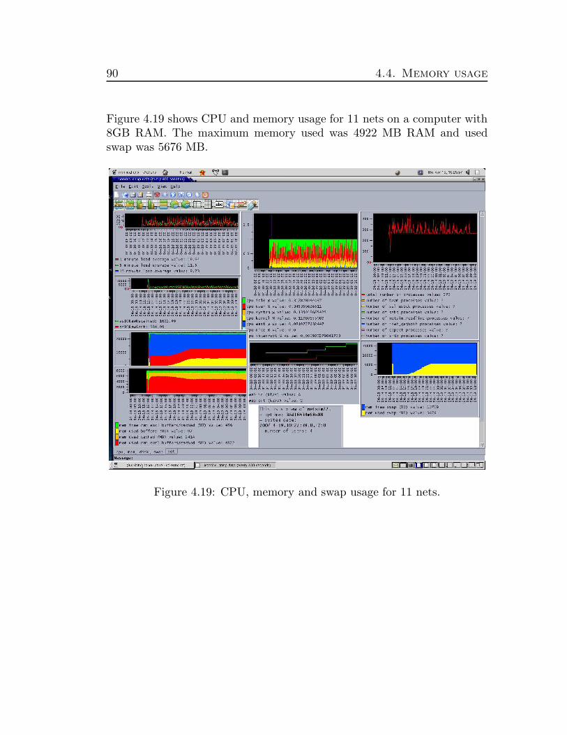
90 4.4. Memory usage
Figure 4.19 shows CPU and memory usage for 11 nets on a computer with8GB RAM. The maximum memory used was 4922 MB RAM and usedswap was 5676 MB.
Figure 4.19: CPU, memory and swap usage for 11 nets.

Results 91
Figure 4.20 shows CPU and memory usage for 12 nets on a computer with8GB RAM. The maximum memory used was 5294 MB RAM and usedswap was 6298 MB.
Figure 4.20: CPU, memory and swap usage for 12 nets.

92 4.4. Memory usage
When using 8 GB RAM the limit for the computer was 10 nets. Therewhere a few minor errors with 10 nets and more and more serious errorsfor 11 nets.
There where 3 lgfmNumRenewalsAttempedTooLate, for 10 nets, see figure4.21. LgfmNumRenewalsAttempedTooLate bigger than zero indicate thatthe load generator is overloaded and do not manages to renewals FM, faultmanagement, subscription in time. lgfmNumRenewalsAttempedTooLate isa measurepoint in NETSim to detect error behaviour.
Figure 4.21: FM for 10 nets.

Results 93
There where no errors for PM for 10 nets, lgpmNumFailedRops are zero,see figure 4.22. LgpmNumFailedRops are a counter for all failures in pre-formance monitoring, like IDL method invocations errors and downloadingdata errors.
Figure 4.22: PM for 10 nets.

94 4.4. Memory usage
For FM for 11 nets the lgfmNumRenewalsAttemptedTooLate was 8, seefigure 4.23.
Figure 4.23: FM for 11 nets.
For PM for 11 nets the lgpmNumFailedRops was 1 and the lgpmNumFaile-dIdlMethodInvocations was 1, see figure 4.24.

Results 95
Figure 4.24: PM for 11 nets.

96 4.4. Memory usage
On the same computer we used for most of the tests we halved the amountof RAM from 8 GB to 4 GB. With 8 GB RAM the limit was 10 nets andwith 4 GB the limit was 6 nets.
Figure 4.25 shows SWUG’s for 6 nets and figure 4.26 shows SWUG’s for 7nets. There were no errors for 6 nets and several errors for 7 nets.
Figure 4.25: SWUG for 6 nets on a computer with 4 GB RAM showing noerrors.

Results 97
Figure 4.26: SWUG for 7 nets on a computer with 4 GB RAM showingseveral errors.

98 4.4. Memory usage

Chapter 5
Discussion, conclusions,recommendations andfuture work
5.1 Discussion and conclusions
In figures 4.1, 4.2 we can see that the difference for get MO attributes be-tween two reference runs is bigger than get MO attributes when we com-pare swap on two partitions with a reference run (original 1).
The figures 4.3 and 4.4 shows that basic create MO for swap on two par-titions is almost the same as for reference run 1 (original 1) and the figureshows that there is a big difference between the two reference runs.
For basic get MO containment short the response times is little lower thanfor the two reference runs but the difference between the two reference runsare as big as the difference between swap on two partitions and the reference
99

100 5.1. Discussion and conclusions
run.
The quartiles 1 and 3 and min95 and max95 in figures 4.7, 4.8 and 4.9 forthe three reference runs shows that there are big variations. If we studythe figures 4.10, 4.11 and 4.12, showing a reference run and a run with twoswap partitions, we can see that the variations are overlapping.
A SWUG is a heavy operation so we studied and compared the times ittook for each SWUG. Figure 4.13 shows the time difference for two referenceruns and figure 4.14 shows the time differences for a reference run and swapon two partitions. As one can see in figure 4.14 the times are overlappingand the max values and min values are almost the same for the two runs.This gives that it is not possible to draw any conclusions that the SWUGtimes for one test run is better than for another test run.
The memory usage is approximately linear for NETSim. On a computerwith 8 GB RAM the limit was 10 nets and on the same computer with 4GB RAM the limit was 6 nets. The size of the swap partition was 16 GBin both cases.
During a run the swap usage increased and leveled out. With 8 GB RAMand 8 nets the maximum memory used was 4521 MB, for 10 nets it was4736 MB RAM, for 11 nets it was 4922 MB RAM and for 12 nets 5294MB RAM. Figure 5.1 shows the memory usage plotted for 8, 10, 11 and 12nets.

Discussion, conclusions, recommendations and future work 101
Figure 5.1: Memory usage for 8, 10, 11 and 12 nets.

102 5.1. Discussion and conclusions
The swap leveled out at 5239 MB for 10 nets, at 5676 MB for 11 nets andat 6298 MB for 12 nets.
Figure 5.2: Swap usage for 8, 10, 11 and 12 nets.
Unfortunately the simulation runs are nondeterministic. This gives that tobe certain one needs to run several simulation runs. This was not practicallypossible because one simulation run took at least 16 hours which gives littlemore than a month for all tests. This and the difference between referenceruns gives an uncertainty in the test results.
To get statistically significant values from the reference runs we calculatea confidence interval for the three IDL methods. From every test runwe get approximately 30 SWUG cycles. Unfortunately we can not use 30samples per test run, because the individual SWUG cycles are codependent.

Discussion, conclusions, recommendations and future work 103
We set confidence level to 0.99, and calculate with one mean value perIDL method from each of the three original test run. For the IDL methodget MO attributes we get the confidence interval [64;77], with arithmeticmean 71, which means that the confidence interval mean ratio is 19%. Forthe IDL method basic get MO containment short we get the confidenceinterval [2.0;2.8],with mean 2.4 and there 35% confidence interval meanratio. For the IDL method basic create MO we get the confidence interval[-1700;5300], with mean 12000 and there 260% confidence interval meanratio. In an attempt to calculate how many test runs we need to getsufficiently small intervals, maximum 5% of the arithmetic mean of theIDL methods. We use the three test runs in round robin fashion to calculatestandard deviation and test for different values of n, see section 2.6. We getn = 8 for get MO attributes, n = 15 for basic get MO containment shortand n = 539 for basic get MO containment short. To run 539 test runs forevery parameter is for obvious reasons not possible, but even 8 test runs isoutside time limits for this thesis.
5.2 Recommendations
The disk usage is not critical and it is needless to spend time on optimisingdisk and file system parameters. The amount of memory used by thesimulations increased approximately linearly with the size of the simulation.The amount of swap space is not critical as long as the swap size is bigenough. This gives that it is possible with more primary memory to increasethe size of the simulation on a computer. The size of the swap space is nota limiting factor.
32-bit Erlang uses less memory than 64-bit Erlang because 64-bit Erlang usepointers whith double size. Primary memory are the biggest limiting factor,indicating that it is better to use 32-bit Erlang for NETSim simulationsthan 64-bit Erlang.
We also recommend to do memory optimisation in NETSim.

104 5.3. Future work
Because the CPU load does not seems to be a limiting factor we recommendusing CPU intensive algorithms instead of memory intensive algorithmswhere it is possible.
5.3 Future work
Today SSL is not included in Erlang core. Instead it is running in a separateprocess. The Erlang core team is working on implementing SSL in Erlang.The current SSL module uses polling and the new implementation supportsKpoll and Epoll. One thing to do in the near future when Erlang with SSLsupport included is released is to ascertain which is the best to use of Epolland Kpoll.
Developing a theoretical model of NETSim regarding disk usage, networkusage, CPU usage, primary memory usage and swap usage makes it possi-ble to do theoretical studies on different parameters’ impact on NETSim.With a theoretical model it is possible to study the parameters’ impact onNETSim without test runs and one can determine which parameter changesthat have no or little impact and run test runs only for the parameters thathave any impact.
Another thing to ascertain is if it is possible to implement trace-driven sim-ulation in NETSim. With trace-driven simulation all activities are recordedand a test run can with all its activities be replayed at a later time. Thisgives a deterministic system that is easier to test. One advantage is that itis possible to run a single test run and compare it with another single testrun based on the same tracking with a changed parameter. In that way itis possible to draw conclusions on a few test runs.
Another advantage with a deterministic system is that it is possible to testseveral parameters at the same time with fractional factorial design. Infraction factorial design we can test combinations of parameters in differenttest run and calculate a single parameters effect of the result and synergyeffects. [32].

Discussion, conclusions, recommendations and future work 105
Further advantage with tracking is that it is possible to save specific testruns, for example test runs known to be problematic.

106 5.3. Future work

Appendix A
Abbreviations
A.1 Abbreviations
ATM Asynchronous Transfer Mode
AUC Authentication Centre
AVC Attribute Value Change
AXE An Ericsson telecom platform.
BBC Best Balanced Choice
BSC Base Station Controller
BTS Base Transceiver Station
CSH Context Sensitive Help
EIR Equipment Identity Register
FAQ Frequently Asked Questions
107

108 A.1. Abbreviations
FTP File Transfer Protocol
GGSN Gateway GPRS Support Node
GMSC Gateway MSC
GPRS General Packet Radio Service
GSM Global System for Mobile
GTP GPRS Tunnel Protocol
GUI Graphical User Interface
HLR Home Location Register
IDL Interface Description Language
IIOP Internet Inter-ORB Protocol (Corba over TCP/IP)
IP Internet Protocol
L1 Layer 1
LSP Logical Scoring of Preferences
MGw Media Gateway
MIB Management Information Base
MO Managed Objects
MSC Mobile Service Switching Center
MTP Message Transfer Protocol
NE Network Element
NME NETSim Management Extension
NMS Network Managing Subsystem
Node B Base Station in UTRAN networks

Abbreviations 109
O&M Operation & Maintenance
OSS Operations and Support System
PFRA Page Frame Reclaiming Algorith
PLMN Public Land Mobile Networks
PM Performance Monitoring
PSTN Public Switched Telephone Network
PSTU Packet Switched Termination Unit
RANAG Radio Access Network Aggregator
RANOS Radio Access Network Operation Support
RBS Radio Base Station.
RNC Radio Network Controller
RNS Radio Network Subsystem
ROAS Region of Acceptable Solutions
RXI Older version of RANAG
SAS Serial Attached SCSI
SCP Service Control Point
SFTP Secure File Transfer Protocol
SGSN Serving GPRS Support Node
SNIA Storage Networking Industry Association
SNMP Simple Network Management Protocol
SRP System Requirement and Parameter tree
SSL Secure Sockets Layer

110 A.1. Abbreviations
SSLIOP Secure Socket Layer Inter-ORB Protocol (IIOP over SSL).
STN Site Transport Node
SWUG SoftWare UpGrade
UE User Equipment
UMTS Universal Mobile Telecommunications System
UTRAN UMTS Terrestrial Radio Access Network
VLR Visitor Location Register
X.25 A standard for packet networks.

Bibliography
[1] NETSim User’s Guide. Ericsson AB, 2006. 1553-CRL 121 03 Uen RevAS 2006-12-14.
[2] Jansson L. Annerberg ULf, Boija Beatrice. OSS-Overview, Operationand Support System Trainee’s Guide. Ericsson Radio Systems AB,1996.
[3] Toskala A. Holma H. WCDMA for UMTS. John Wiley & Sons Ltd.,2001.
[4] Gunnarsson Frida Knutsson Bjorn, Bjorsson Anders. Radio AccessNetwork ( UTRAN ) Modeling for Heterogenous Network Simulations,A Brief Description. 2003.
[5] Johansson Christer Hameleers Heino. IP Technology inWCDMA/GSM core networks. Ericsson AB, 2002. EricssonReview No. 1, 2002.
[6] UMTS Overview. Ericsson AB, 1999. ERA/UX/T-99:108 Rev PA1.
[7] Althoff M. P. Walke B., Seidenberg P. UMTS The Fundamentals. JohnWiley & Sons Ltd., 2003.
[8] Ericsson Tomas Narup Micael, Helgeson Claes. Att forsta Telekommu-
nikation 1. Studentlitteratur, Ericsson Telecom AB, Telia AB, 1997.SV/LZT 101 1402R1B.
111

112 BIBLIOGRAPHY
[9] NETSim basics course material. Ericsson AB, 2006. From 2006-04-10.
[10] The NETSim programming course material. Ericsson AB, 2007. From2007-03-16.
[11] NETSim System Administrator’s Guide. Ericsson AB, 2007. 1543-CRL 121 03 Uen Rev AF 2007-02-23.
[12] PerfCons How To Test. Ericsson AB, Fetched 2007-03-02. From anEricsson-internal wiki.
[13] Common RAID Disk Data Format Specification, Re-vision 1.2 with Errata A Applied. SNIA Stor-age Networking Industry Associattion, 2007-08-29.http://www.snia.org/tech activities/standards/curr standards/ddf/SNIA-DDFv1.2 with Errata A Applied.pdf.
[14] Holmquist Bjorn Blom Gunnar. Statistikteori med tillampningar. Stu-dentlitteratur, 1998.
[15] Cesati Marco Bovet Daniel P. Understanding the Linux kernel 3 ed.
O’Reilly, 2006.
[16] Florian Buchholz. The structure of the Reiser file sys-tem, Fetched 2007-04-23. http://homes.cerias.purdue.edu/ flo-rian/reiser/reiserfs.php.
[17] Naujok Barry. XFS Filesystem Structure. Silicon Graphics, 2006. 2ndEdition, Revision 2.
[18] Best Steve. JFS overview. IBM, January 2000.
[19] Rivest L. Ronald H. Cormen Thomas, Leiserson E. Charles. Intro-
ductions to algorithms second edition. McGraw-Hill Companies Inc.,Fourth printing 2003.
[20] Hans Reiser. ReiserFS v.3 Whitepa-per. namesys.com, Fetched 2007-04-23.http://web.archive.org/web/20030621014013/namesys.com/content table.html.

[21] Koren Dan Mostek Jim, Earl William. Porting the SGI XFS FileSystem to Linux. Silicon Graphics.
[22] Kleikamp Dave Best Steve. JFS layout. IBM Linux Technology Center,May 2000.
[23] Best Steve. JFS Log, How the Journaled File System performs logging.IBM Linux Technology Center, October 2000.
[24] Kernel changelogs from 2.6.0 to 2.6.21.
[25] Gagne Greg Silberschatz Avi, Galvin Peter. Applied Operating System
Concepts. John Wiley & Sons Inc., 2000.
[26] Documentation/filesystems/proc.txt from the Linux kernel source treefor kernel 2.6.8.
[27] Documentation/sysctl/vm.txt from the Linux kernel source tree forkernel 2.6.8.
[28] Blom Gunnar. Sannolikhetsteori och statistikteori med tillampningar.Studentlitteratur, 1980.
[29] Wittmeyer-K Linde Elden Lars. Numeriska berakningar - analys och
illustrationer med MATLAB. Studentlitteratur, 2001.
[30] MAY2073RC MAY2036RC HARD DISK DRIVES PROD-UCT/MAINTENANCE MANUAL. FUJITSU, 2005. C141-E230-01EN.
[31] Linus Torvalds. Re: [ext3][kernels >= 2.6.20.7 at least] KDE goingcomatose when FS is under heavy write load (massive starvation),Fetched 2007-04-27. http://lkml.org/lkml/2007/4/27/289.
[32] Runesson Per Berling Tomas. Efficient Evaluation of MultifactorDependent System Performance Using Fractional Factorial Design,september 2003. IEEE Transactions on Software Engineering, Vol 29,No. 9.

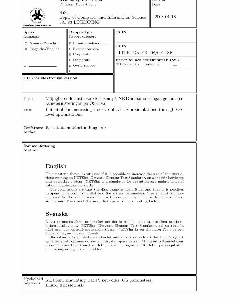
Avdelning, Institution
Division, DepartmentDatum
Date
Sprak
Language
2 Svenska/Swedish
4 Engelska/English
2
Rapporttyp
Report category
2 Licentiatavhandling
4 Examensarbete
2 C-uppsats
2 D-uppsats
2 Ovrig rapport
2
URL for elektronisk version
ISBN
ISRN
Serietitel och serienummer
Title of series, numberingISSN
Titel
Title
Forfattare
Author
Sammanfattning
Abstract
Nyckelord
Keywords
EnglishThis master’s thesis investigates if it is possible to increase the size of the simula-tions running on NETSim, Network Element Test Simulator, on a specific hardwareand operating system. NETSim is a simulator for operation and maintenance oftelecommunication networks.
The conclusions are that the disk usage is not critical and that it is needlessto spend time optimizing disk and file system parameters. The amount of mem-ory used by the simulations increased approximately linear with the size of thesimulation. The size of the swap disk space is not a limiting factor.
SvenskaDetta exsamensarbete undersoker om det ar mojligt att oka storleken pa simu-leringskorningar av NETSim, Network Element Test Simulator, pa en specifikhardvaru- och operativsystemsplattform. NETSim ar en simulator for styr ochovervakning av telekomnatverk.
Slutsatserna ar att diskanvandandet inte ar kritiskt och att det ar onodigt attagna tid at att optimera disk- och filsystemsparametrar. Minnesutnyttjandet okarapproximativt linjart med storleken pa simuleringarna. Storleken pa swapdiskenar inte nagon begransande faktor.
SaS,Dept. of Computer and Information Science581 83 LINKOPING
2008-01-18
—
LITH-IDA-EX--08/001--SE
—
Potential for increasing the size of NETSim simulations through OS-level optimizations
Mojligheter for att oka storleken pa NETSim-simuleringar genom pa-rameterjusteringar pa OS-niva
Kjell Enblom,Martin Jungebro
NETSim, simulating UMTS networks, OS parameters,Linux, Ericsson AB

116

LINKÖPING UNIVERSITY
ELECTRONIC PRESS
Copyright
Svenska
Detta dokument halls tillgangligt pa Internet - eller dess framtida ersattare - under 25 ar franpubliceringsdatum under forutsattning att inga extraordinara omstandigheter uppstar.
Tillgang till dokumentet innebar tillstand for var och en att lasa, ladda ner, skriva ut enstakakopior for enskilt bruk och att anvanda det oforandrat for ickekommersiell forskning och forundervisning. Overforing av upphovsratten vid en senare tidpunkt kan inte upphava dettatillstand. All annan anvandning av dokumentet kraver upphovsmannens medgivande. Foratt garantera aktheten, sakerheten och tillgangligheten finns det losningar av teknisk ochadministrativ art.
Upphovsmannens ideella ratt innefattar ratt att bli namnd som upphovsman i den omfattningsom god sed kraver vid anvandning av dokumentet pa ovan beskrivna satt samt skydd mot attdokumentet andras eller presenteras i sadan form eller i sadant sammanhang som ar krankandefor upphovsmannens litterara eller konstnarliga anseende eller egenart.
For ytterligare information om Linkoping University Electronic Press se forlagets hemsidahttp://www.ep.liu.se/
English
The publishers will keep this document online on the Internet - or its possible replacement -for a period of 25 years from the date of publication barring exceptional circumstances.
The online availability of the document implies a permanent permission for anyone to read,to download, to print out single copies for your own use and to use it unchanged for anynon-commercial research and educational purpose. Subsequent transfers of copyright cannotrevoke this permission. All other uses of the document are conditional on the consent of thecopyright owner. The publisher has taken technical and administrative measures to assureauthenticity, security and accessibility.
According to intellectual property law the author has the right to be mentioned when his/herwork is accessed as described above and to be protected against infringement.
For additional information about the Linkoping University Electronic Press and its proce-dures for publication and for assurance of document integrity, please refer to its WWW homepage: http://www.ep.liu.se/
c© Kjell Enblom,Martin JungebroLinkoping, 18th January 2008