reactor reference and tutorials
TRANSCRIPT

www.discreet.com
REFERENCE AND TUTORIALS
21100-010000-5020AJuly 2002

Copyright © 2002 Autodesk, Inc. All Rights Reserved
This publication, or parts thereof, may not be reproduced in any form, by any method, for any purpose.
AUTODESK, INC. MAKES NO WARRANTY, EITHER EXPRESSED OR IMPLIED, INCLUDING BUT NOT LIMITED TO ANY IMPLIED WAR-RANTIES OF MERCHANTABILITY OR FITNESS FOR A PARTICULAR PURPOSE, REGARDING THESE MATERIALS AND MAKES SUCH MATERIALS AVAIL-ABLESOLELY ON AN "AS-IS"BASIS. IN NO EVENT SHALL AUTODESK, INC. BE LIABLE TO ANYONE FOR SPECIAL, COLLATERAL, INCIDENTAL, OR CONSEQUENTIAL DAMAGES IN CONNECTION WITH OR ARISING OUT OF PURCHASE OR USE OF THESE MATERIALS. THE SOLE AND EXCLUSIVE LIA-BILITY TO AUTODESK, INC., REGARDLESS OF THE FORM OF ACTION, SHALL NOT EXCEED THE PURCHASE PRICE OF THE MATERI-ALS DESCRIBED HEREIN.Autodesk, Inc. reserves the right to revise and improve its products as it sees fit. This publication describes the state of this product at the time of its publication, and may not reflect the product at all times in the future.
Autodesk Trademarks:The following are registered trademarks of Autodesk, Inc., in the USA and/or other countries: 3D Plan, 3D Props, 3D Studio, 3D Studio MAX, 3D Studio VIZ, 3DSurfer, ActiveShapes, ActiveShapes (logo), Actrix, ADE, ADI, Advanced Modeling Extension, AEC Authority (logo), AEC-X, AME, Animator Pro, Animator Studio, ATC, AUGI, AutoCAD, AutoCAD Data Extension, AutoCAD Development System, AutoCAD LT, AutoCAD Map, Autodesk, Autodesk Animator, Autodesk Inventor, Autodesk (logo), Autodesk MapGuide, Autodesk University, Autodesk View, Autodesk WalkThrough, Autodesk World, AutoLISP, AutoShade, AutoSketch, AutoSurf, AutoVision, Biped, bringing information down to earth, CAD Overlay, Character Studio, Cinepak, Cinepak (logo), Codec Central, Combustion, Design Companion, Design Your World, Design Your World (logo), Discreet, Drafix, EditDV, Education by Design, Generic, Generic 3D Drafting, Generic CADD, Generic Software, Geodyssey, Heidi, HOOPS, Hyperwire, i-drop, Inside Track, Kinetix, MaterialSpec, Mechanical Desktop, Media Cleaner, MotoDV, Movie Cleaner Pro, Multimedia Explorer, NAAUG, ObjectARX, Office Series, Opus, PeopleTracker, PhotoDV, Physique, Planix, Powered with Autodesk Technology, Powered with Autodesk Technology (logo), RadioRay, Rastation, Revit, Softdesk, Softdesk (logo), Solution 3000, Terran Interactive, Texture Universe, The AEC Authority, The Auto Architect, TinkerTech, Videofusion, VISION*, Visual LISP, Volo, Web-Motion, WHIP!, WHIP! (logo), Wood-bourne, WorkCenter, and World-Creating Toolkit.
The following are trademarks of Autodesk, Inc., in the USA and/or other countries: 3D on the PC, 3ds max, ACAD, Advanced User Interface, AME Link, Auto-CAD
Architectural Desktop, AutoCAD Learning Assistance, AutoCAD LT Learning Assistance, AutoCAD Simulator, AutoCAD SQL Extension, AutoCAD SQL Interface, Autodesk Device Interface, Autodesk Map, Autodesk Software Developer’s Kit, Autodesk Streamline, Autodesk View DwgX, AutoFlix, AutoSnap, AutoTrack, Built with ObjectARX (logo), Burn, Buzzsaw, Buzzsaw.com, Cinestream, Cleaner, Cleaner Central, ClearScale, Colour Warper, Concept Studio, Con-tent Explorer, cornerStone Toolkit, Dancing Baby (image), DesignCenter, Design Doctor, Designer’s Toolkit, DesignProf, DesignServer, DWG Linking, DXF, Extending theDesignTeam,FLI,FLIC,GDXDriver,gmax,gmax(logo),gmax ready (logo),Heads-upDesign,Home Series,Intelecine,IntroDV,jobnet,Kinetix (logo), Live Sync, ObjectDBX, onscreen onair online, Ooga-Chaka, Plans & Specs, Plasma, Plugs and Sockets, PolarSnap, ProjectPoint, Reactor, Real-Time Roto, Render Queue, Sparks, The Dancing Baby, Transform Ideas Into Reality, Visual Syllabus, VIZable, and Where Design Connects.
Autodesk Canada Inc. Trademarks: The following are registered trademarks of Autodesk Canada Inc. in the USA and/or Canada, and/or other countries: discreet, fire, flame, flint, flint RT, frost, glass, inferno, MountStone, riot, river, smoke, stone, stream, vapour, wire. The following are trademarks of Autodesk Canada Inc., in the USA, Canada, and/or other countries: backburner, backdraft, heatwave, Multi-Master Editing.
Third-Party Trademarks:All other brand names, product names or trademarks belong to their respective holders.
Third-Party Software Program Credits: © 2002 Microsoft Corporation. All rights reserved.ACIS © 1989–2002, Spatial Corp. AnswerWorks ® Copyright © 1997–2002 WexTech Systems, Inc. Portions of this software © Lernout & Hauspie, Inc. All rights reserved.Certain patents licensed from Viewpoint Corporation.InstallShield™ Copyrighted © 2002 InstallShield Software Corporation. All rights reserved.LLicensing Technology Copyright © Macrovision Corp. 1996–2002. Portions Copyrighted © 1989–2002 mental images GmbH & Co. KG Berlin, Germany.Portions Copyrighted © 2002 Blur Studio, Inc. Portions Copyrighted © 2002 Intel Corporation. Portions developed by Digimation, Inc. for the exclusive use of Autodesk, Inc. Portions developed by Lyric Media, Inc. for the exclusive use of Autodesk, Inc.Portions of this software are based on the copyrighted work of the Independent JPEG Group. reactor™ is produced for Discreet, a division of Autodesk, Inc., by Havok.com, Inc. Copyright © 1999–2002 Havok.com, Inc. All Rights Reserved. Please see www.havok.com for details. Wise Installation System for Windows Installer © 2002 Wise Solutions, Inc. All rights reserved.
GOVERNMENT USE: Use, duplication, or disclosure by the U.S. Government is subject to restrictions as set forth in FAR 12.212 (Commercial Computer Soft-ware-Restricted Rights) and DFAR 227.7202 (Rights in Technical Data and Computer Software), as applicable.
1 Welcome . . . . . . . . . . . . . . . . . . . . . . . . 1Getting Started . . . . . . . . . . . . . . . . . . . . . . . . . . . 2Advanced Display Features . . . . . . . . . . . . . . . . 5
2 Rigid Bodies . . . . . . . . . . . . . . . . . . . . . . 7About This Tutorial . . . . . . . . . . . . . . . . . . . . . . . 7Creating a Rigid Body Simulation. . . . . . . . . . . 8Rigid Body Properties . . . . . . . . . . . . . . . . . . . . 10Rigid Collection Properties. . . . . . . . . . . . . . . . 11
3 Convex and Concave Objects . . . . . 13About This Tutorial . . . . . . . . . . . . . . . . . . . . . . 14Performing a Convexity Test . . . . . . . . . . . . . . 14Treating an Object as Convex. . . . . . . . . . . . . . 14Treating an Object as Concave. . . . . . . . . . . . . 16Building a Compound Rigid Body . . . . . . . . . 17More About Proxies. . . . . . . . . . . . . . . . . . . . . . 18
4 Soft Bodies . . . . . . . . . . . . . . . . . . . . . . 21About These Tutorials . . . . . . . . . . . . . . . . . . . . 21Creating a Soft Body Simulation . . . . . . . . . . . 22More Advanced Soft Bodies . . . . . . . . . . . . . . . 23Freeform Deformation. . . . . . . . . . . . . . . . . . . . 24
5 Cloth . . . . . . . . . . . . . . . . . . . . . . . . . . . 27About This Tutorial . . . . . . . . . . . . . . . . . . . . . . 27Creating a Cloth Simulation . . . . . . . . . . . . . . . 28Advanced Cloth Properties . . . . . . . . . . . . . . . 30Limitations of the Cloth Model . . . . . . . . . . . . 31
6 Rope . . . . . . . . . . . . . . . . . . . . . . . . . . . 33About These Tutorials. . . . . . . . . . . . . . . . . . . . 33Creating a Rope Simulation . . . . . . . . . . . . . . . 33
7 Water . . . . . . . . . . . . . . . . . . . . . . . . . . 37About This Tutorial . . . . . . . . . . . . . . . . . . . . . . 37Adding Water to a Scene . . . . . . . . . . . . . . . . . 38
8 Constraints . . . . . . . . . . . . . . . . . . . . . . 41About This Tutorial . . . . . . . . . . . . . . . . . . . . . . 41Springs and Dashpots . . . . . . . . . . . . . . . . . . . . 42Adding a Spring to a Simulation . . . . . . . . . . . 42Adding a Dashpot . . . . . . . . . . . . . . . . . . . . . . . 44Constraints . . . . . . . . . . . . . . . . . . . . . . . . . . . . . 45The Toy Car . . . . . . . . . . . . . . . . . . . . . . . . . . . . 49
9 Actions . . . . . . . . . . . . . . . . . . . . . . . . . 53About This Tutorial . . . . . . . . . . . . . . . . . . . . . . 53The Actions . . . . . . . . . . . . . . . . . . . . . . . . . . . . . 53Adding Actions to Scenes. . . . . . . . . . . . . . . . . 54
10 Animation . . . . . . . . . . . . . . . . . . . . . . 59About This Tutorial . . . . . . . . . . . . . . . . . . . . . . 59Creating a Simple Animation. . . . . . . . . . . . . . 59Mixing Keyframes and Physical
Animation I . . . . . . . . . . . . . . . . . . . . . . . . . . . 61Mixing Keyframes and Physical
Animation II. . . . . . . . . . . . . . . . . . . . . . . . . . . 62Deforming Meshes. . . . . . . . . . . . . . . . . . . . . . . 62Keyframe Reduction . . . . . . . . . . . . . . . . . . . . . 63Interactive Modification . . . . . . . . . . . . . . . . . . 64

Contentsiv
11 MAXScript and reactor . . . . . . . . . . . . 65reactor Objects . . . . . . . . . . . . . . . . . . . . . . . . . . 65Setting Physical Properties . . . . . . . . . . . . . . . . 69Running Scripts . . . . . . . . . . . . . . . . . . . . . . . . . 72
12 World Scale . . . . . . . . . . . . . . . . . . . . . 75World Scale . . . . . . . . . . . . . . . . . . . . . . . . . . . . . 75Collision Tolerance . . . . . . . . . . . . . . . . . . . . . . 76
13 Advanced Simulation Properties . . . . 77
Appendix: Physics Primer . . . . . . . . . . 79Physical Simulation . . . . . . . . . . . . . . . . . . . . . . 79Collision Detection. . . . . . . . . . . . . . . . . . . . . . . 90Physical Units and Values . . . . . . . . . . . . . . . 101Next Steps . . . . . . . . . . . . . . . . . . . . . . . . . . . . . 106
Glossary . . . . . . . . . . . . . . . . . . . . . . . 109
Index. . . . . . . . . . . . . . . . . . . . . . . . . . 115

Welcomereactor™ is a plug-in for 3ds max™ designed to allow artists and animators to control and simulate complex physical scenes with ease. reactor supports fully integrated rigid and soft body dynamics, cloth simulation and fluid simulation. It can simulate constraints and joints for articulated bodies. It can also simulate physical behaviors such as wind and motors. You can use all of these features to create rich dynamic environments.
Once a designer creates an object in 3ds max, they can assign physical properties to it. Properties could include characteristics such as mass, friction, and elasticity. Objects can be fixed, free, attached to springs, or attached together using a variety of constraints. By assigning physical characteristics to objects, you can model real-world scenarios quickly and easily, and these can then be simulated to produce physically accurate keyframed animations.
With reactor, you can preview scenes quickly using the real-time simulation display window. This window allows you to test and play with a scene interactively. You can alter positions of all physical objects in the scene, dramatically reducing the design time. You can then transfer the scene back into 3ds max with a single key-click, while retaining all the properties needed for the animation.
The reactor plug-in frees designers and animators from having to hand-animate time consuming secondary effects, like exploding buildings or draping curtains. The plug-in also supports all standard 3ds max features such as keyframes and skinning, so you can use both conventional and physical animation in the same scene. Convenient utilities (such as automatic keyframe reduction) let you tweak and alter the physically generated parts of an animation after it has been generated.
The remainder of this document describes each of the plug-in's features in detail. It also contains detailed tutorials to show you how to get the most from reactor.
Further files and tutorials are available at www.discreet.com

Chapter 1: Welcome2
Getting StartedThe first thing you need to do to use the plug-in is to display the reactor panel. The panel contains the options for your simulation, and using it, you can apply physical properties to the objects in your scene.
Figure 1.1.1.
To display the reactor panel:
1. Select the Utilities command panel.
2. Click the More button.
3. Select reactor from the list on the Utilities dialog box (Figure 1.1.1).
4. Click the OK button.
The reactor plug-in contains several extended versions of the default user interfaces, which contain a reactor toolbar and a reactor quad menu. The quad menu is accessible in any viewport using Shift+Alt plus the right mouse button. Both the quad menus and the toolbar provide shortcuts for many of the reactor functions. This manual does not use the toolbar buttons or quad menu functions for its tutorials.
However, nearly all of the tasks performed within the tutorials have a toolbar and menu equivalent. Detailed below is an explanation for each symbol in the toolbar. This manual discusses all of these functions.
Add a Rigid Body Collection.
Add a Soft Body Collection.
Apply the Soft Body modifier.
Add a Constraint Solver.
Add a Point-to-Nail Constraint.
Add a Spring.
Add a Wind Action.
Add a Motor Action.
Open the Preview window.
Analyze World.
Deforming Mesh.
Add a Rope Collection.
Add a Cloth Collection.
Apply the Cloth modifier.

Getting Started 3
Apply the Attach-to-Rigid Body
modifier.
Add a Point-to-Point constraint.
Add a Point-to-Path constraint.
Add a Dashpot.
Add Water.
Add a reactor Plane.
Perform Simulation.
Toy Car.
Fracture Action.
Apply a Rope modifier.
Installing the ToolbarTo install the reactor toolbar:
1. Choose Load Custom UI from the Customize menu
2. Select the one of the .cui files containing reactor in its name. These files provide customized reactor versions of the standard 3ds max user interfaces. Alternatively, if you already have a customized UI you can merge the reactor toolbar into it using the merge tool, available at www.discreet.com.Basic Steps
There are usually six steps to creating and previewing a scene with the plug-in:
1. Creating your scene in 3ds max.
2. Applying physical properties to the objects in your scene using the Properties section of the reactor rollout.
3. Creating collections to which you add objects.
4. Creating any systems you want in the scene.
5. Adding cameras and lights.
6. Previewing the simulation.
You do not have to follow these steps in this specific order. It is often practical to create a collection before you add any objects to the scene, for example.
The menu options for the display window are as follows:
Key Function
P Plays or pauses the scene
R Resets the scene to its original position
LMB (Left Mouse Button) Rotates the scene around the origin
MMB Hold the middle button to pan the camera
RMB (Right Mouse Button) Picks objects. You can pick up objects by right clicking on them. You then drag the object using a spring connected to the mouse pointer and to the selected object.
Arrows Lets you move in, out, left and right
F Displays the Frame Rate
Chapter 1: Welcome4
SimulationPlay/Pause—Allows you to play or pause the simulation at any time. When paused, all simulation ceases (objects are frozen in space and time) but you can still change the camera position to view any objects in the scene. You can also step a paused scene forward in single time increments to view simulation progression more accurately. You can then get the layout of the objects in 3ds max to mirror the current simulation world when used in conjunction with the Update Max function. This is particularly useful if you use the preview window to aid object positioning in 3ds max.
Reset—Resets the simulation to either start or updated positions in 3ds max.
DisplayMax Mouse Mode—Toggles between the two mouse modes. The Max Mouse Mode is on by default.
Background Color—Sets the background color for the display window.
Camera Setting—Allows you to set both the distance of the two clipping planes and the field of view for the camera.
Flashlight—Switches the default flashlight on or off. The flashlight is turned on by default in lightless scenes.
Fog—Toggles fog on and off.
Anti-Aliasing—Toggles anti-aliasing on and off, but only if supported by your graphics card.
Textures—Toggles between the default colors and textures from 3ds max.
Culling—Toggles whether or not to cull the back faces.
Lighting, Shadows—Toggles lighting effects/shadows on and off.
Toggle Display On/Off—Allows you to see the display's effect on the frame rate.
PhysicsReal Time—Runs a simulation in real-time, using actual elapsed clock time.
Fixed Step—Allows you to specify the size of time-step between each physical evaluation. The updated simulation is only available for display after each time-step is taken. If this is a User Defined Step then the value is defined by the 3ds max animation parameters. Smaller timesteps imply more accurate the physics.
Substeps—Allows you to specify the number of physical sub-steps taken internally during each evaluation. This controls the accuracy of each time-step evaluation. A larger number of sub-steps mean more accurate time-steps, and more accurate physics.
Gravity—Toggles gravity on and off.
GeometryFaces—Toggles whether to display the faces of the objects in a scene.
Edges—Shows the edges of the objects in a scene.
Sim Edges—Shows the geometries that are actually being simulated. In reactor, complex geometries can be displayed while the physics actually simulates a much simpler geometry.

Advanced Display Features 5
Max menuUpdate Max—Translates the positions and internal states of the objects in the simulation window back into 3ds max.
Use Max Parameters—Resets timestep and substeps to the values determined by the Animation rollout parameters (used when the preview window was created).
Advanced Display FeaturesAll the information contained in this rollout is only useful for the Preview In Window feature. It does not affect 3ds max animations, as 3ds max already has all this information, and of course uses it. Figure 1.4.1 shows the advanced features of the Display rollout.
Camera
The plug-in allows you to choose a camera in the scene as the display camera, which reactor then uses when the preview starts.
Lights Feature
You can select up to 6 lights to add to the simulation. If you select none, then a default flashlight is used.
The light properties useful for real-time simulation are used and exported. This includes properties such as position, orientation, color, falloff, etc. If a light in
3ds max is linked to a rigid body in the simulation, then the light remains linked during the simulation. It moves and rotates with the rigid body.
Figure 1.4.1
Shadows
The preview window displays real-time shadows. Information associated with these shadows is also exported. While shadows add a lot of realism to scenes, they are expensive and have some limitations. In reactor, shadows can only be cast onto a plane, and can only be cast by lights in the simulation. The default flashlight doesn't cast shadows. You can use these steps to create shadows:
1. Choose the lights from which you want to cast shadows, open their Modify Branch options and select their Casts shadows checkboxes.
Chapter 1: Welcome6
2. Select Cast Shadows on Plane in the Display rollout.
3. Click the Pick button and select the plane onto which you want to cast shadows. You can use either a plane object or any other object. The plane used is the one defined by the object local coordinates (located at the pivot and with its normal pointing to the Z direction). If you are casting shadows over another object in the simulation, ensure that the plane where you cast the shadows is slightly above that floor or ground, so shadows appear perfectly over the floor and not covered by it.
4. Disable the shadow casting for objects that don't cast shadows by deselecting their Cast shadows checkboxes. This box is found in the Properties section of each 3ds max object.
Texture Quality
You can choose the quality of texture maps. A higher number of pixels can improve make your scene's appearance, but also slow rendering and increase file sizes in exports. Values of 128 or 256 are usually fine.
The mouse spring
In the preview window, you can use the mouse to interact with the scene. Right clicking on a rigid body applies a spring between the mouse pointer and the selected body. You can interact with the objects by moving them, throwing them away, etc.
You can set the strength, rest length and damping of the spring from the Display rollout of the plug-in. You can increase the strength if you find it difficult to move the objects, or decrease it if objects move too fast. For an explanation of the parameters, see the Springs & Dashpots section.
Rigid BodiesThe most basic components in any scene are usually rigid bodies. Rigid bodies are literally objects that do not change shape. Rigid bodies are commonly used to represent a wide variety of scene components. A rigid body can be anything from a teacup to a table to a very big rock. Rigid bodies are also commonly used as starting points for other kinds of objects. For example, you can create a soft body (a deformable type of object) from a rigid body.
reactor™ handles bodies using entity collections. Entity collection is a specially defined term used to describe the main components of a simulation. A rigid body collection is an example of an entity collection, and rigid bodies are members of rigid body collections. Collections are necessary for the purposes of solving and simulating object movement and interaction.
There are also many physical properties that you can assign to a rigid body. These properties describe the behavior of the body in a scene. They determine the mass, friction, elasticity and other properties of the body.
About This TutorialThis tutorial introduces the reactor plug-in to new users. It describes how to use reactor to assign physical properties to objects in a simple scene by treating them as rigid bodies. It also describes how to view and interact with the scene in the reactor display window. When you complete this tutorial, you will be able to:
• Create a rigid body collection.
• Add objects to a rigid body collection.
• Add a camera to a scene.
• Assign physical properties to objects in a scene.
• Simulate a scene.

Chapter 2: Rigid Bodies8
In the Scenes folder in the reactor directory, there are two files associated with this tutorial. They show how your scene should appear at the start and at the end of the tutorial. They are called TutorialOneStart.max and TutorialOneEnd.max.
Creating a Rigid Body SimulationWhen you create a simple scene, you must add the objects that you want to model in reactor to a rigid body collection. Creating a rigid body collection is usually the first step in using reactor.
A rigid body collection is an object used to contain a set of rigid bodies. reactor can only physically simulate rigid-bodies if they are members of a rigid body collection.
To create a simple rigid body simulation:
1. Create a scene containing a couple of simple objects. For example, you create a box with a b ox and sphere above it (Figure 2.2.1). If you don't want to create the scene you can load TutorialOneStart.max
2. Select the Helpers icon from the Create command panel.
3. Select reactor from the Helpers drop-down menu.
4. Click the RBCollection button in the Object Type rollout.
5. Click any of the view panes to place the rigid body collection symbol within your scene.
Figure 2.2.1
You can move the symbol around the scene, as its position does not affect reactor. It is better to keep the collection symbol away from your objects to avoid cluttering the scene.
You can accept the default name for the rigid body collection, or you can assign a new name. You may add new objects to a rigid body collection as you create it. You can also add objects at any point after the creation of the collection.
Adding Bodies to a Rigid Body CollectionYou need to add your objects to the rigid body collection. You can do that in the following way:
1. Select the collection.
2. Click the Modify tab in 3ds max and expand the RBCollection Properties (Figure 2.2.2) rollout.
3. Click the Add button.
4. Use the displayed Select Rigid Bodies dialog box to select the objects that you want to add to the rigid body collection.

Creating a Rigid Body Simulation 9
Alternatively, you can click the Pick button and select individual objects from the view panes.
You now have a rigid collection that you can simulate.
Figure 2.2.2
Adding a CameraThe next step for the simulation is to add a camera to the scene. This means that you can specify the initial view for the display, which removes the need to reposition your viewpoint each time the simulation is run. The 3ds max documentation describes cameras in more detail.
1. Click the Lights and Cameras tab.
2. Click the Targeted Camera icon.
3. Click any of the view panes to place the camera within your scene.
You can adjust the camera so that it is positioned appropriately.
If you have decided to use your own camera for simulation, you should expand the Display rollout from the reactor utility and associate your camera with the display. Click the None button beside the word Camera and then select your camera. This associates the camera with the display.
You can also add lights to your simulation. You may add up to six lights to the scene. You can add them to the simulation using the Lights section in the Display rollout. It is not necessary to do this since reactor automatically adds its own light in the preview window. This light is only visible in the preview window, and only added if you specify no other 3ds max lights for simulation.
reactor uses a default camera to display a scene in the reactor display window, so this is unnecessary, and this section can be skipped if you wish to use this default camera.
Assigning Physical PropertiesWhen you have a number of rigid bodies in a rigid body collection, you can assign physical properties to each of the bodies. In fact, you can assign properties at any time before simulation. Physical properties are characteristics such as mass, elasticity, and friction. Each property has a default value.
Figure 2.2.3
1. Click the Utilities command panel.
2. Expand the Properties rollout from the reactor utility.
Chapter 2: Rigid Bodies10
3. Select one of the rigid bodies from any of the view panes.
4. Assign appropriate physical properties to the rigid body by entering values in the Mass, Elasticity and Friction fields. (Figure 2.2.3)
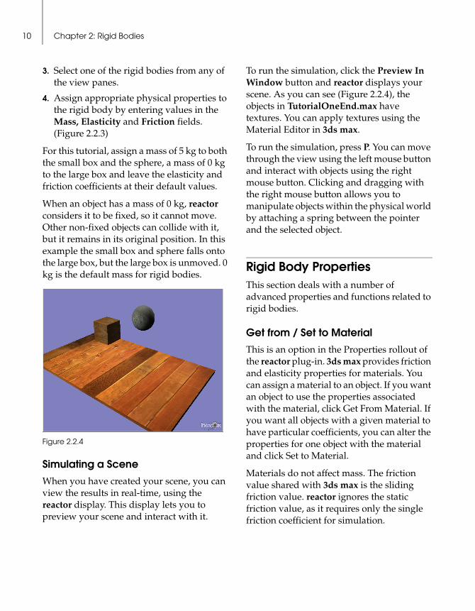
For this tutorial, assign a mass of 5 kg to both the small box and the sphere, a mass of 0 kg to the large box and leave the elasticity and friction coefficients at their default values.
When an object has a mass of 0 kg, reactor considers it to be fixed, so it cannot move. Other non-fixed objects can collide with it, but it remains in its original position. In this example the small box and sphere falls onto the large box, but the large box is unmoved. 0 kg is the default mass for rigid bodies.
Figure 2.2.4
Simulating a SceneWhen you have created your scene, you can view the results in real-time, using the reactor display. This display lets you to preview your scene and interact with it.
To run the simulation, click the Preview In Window button and reactor displays your scene. As you can see (Figure 2.2.4), the objects in TutorialOneEnd.max have textures. You can apply textures using the Material Editor in 3ds max.
To run the simulation, press P. You can move through the view using the left mouse button and interact with objects using the right mouse button. Clicking and dragging with the right mouse button allows you to manipulate objects within the physical world by attaching a spring between the pointer and the selected object.
Rigid Body PropertiesThis section deals with a number of advanced properties and functions related to rigid bodies.
Get from / Set to MaterialThis is an option in the Properties rollout of the reactor plug-in. 3ds max provides friction and elasticity properties for materials. You can assign a material to an object. If you want an object to use the properties associated with the material, click Get From Material. If you want all objects with a given material to have particular coefficients, you can alter the properties for one object with the material and click Set to Material.
Materials do not affect mass. The friction value shared with 3ds max is the sliding friction value. reactor ignores the static friction value, as it requires only the single friction coefficient for simulation.

Rigid Collection Properties 11
Convex / ConcaveThis affects the way bodies collide with other bodies, and the accuracy of the simulation. This is dealt with in the next chapter.
Display ProxiesYou can optimize the display frame rate within the reactor preview window by using display proxies. A display proxy literally means that you use one object as a proxy for the display of another. Display proxies are rarely useful for animation, and so this section only really concerns uses for real-time preview of large scenes.
With rendered animation, you can devote as much time to physics and display as you require, but real-time requires a different approach. You might use a detailed display proxy with simple physics for complicated interactions or a simple display proxy for commonly repeated objects where the display reduces the speed of the simulation.
Figure 2.3.1
For example, if you have a length of chain, you could simulate each link as a thin hollow box, but use the display proxy of a detailed torus (Figure 2.3.1).
To use a display proxy, select the object for which you want to use a proxy, check the Proxy option in the Properties rollout, click the None button and select the object you want to use as the display proxy.
If you select Display Children, then all children of this object, linked though 3ds max's internal hierarchy, are displayed. You may need to uncheck this box if you get children displaying more than once.
Rigid Collection PropertiesIn the Modify panel for a rigid collection there are two rollouts, RBCollection Properties and Advanced. This section details the extra features not yet mentioned in these two rollouts.
Disabling Collections Below the list of bodies contained in the collection is a check box labeled Disabled. If any collection is disabled, it is not included in simulation. Any collection you create is automatically included in simulation by default.
DisplayIt is possible to customize how you display all reactor icons in the 3ds max viewports.
ODE SolversYou can choose which Ordinary Differential Equation (ODE) solver to use for a particular collection. The four options are:

Chapter 2: Rigid Bodies12
Euler
The simplest ODE solver and very fast but not sufficient for complicated systems.
Back-Euler
Slightly more accurate than Euler, but performs worse for spring systems. Interactive scenes that require a mouse spring should use Euler or Runge-Kutta solvers.
Midpoint
Has a level of accuracy similar to that of Back-Euler, but also does not solve spring systems sufficiently.
Runge-Kutta
This is the most accurate solver in the system and is used in complicated systems, springs and constraints. Because of its improved accuracy it requires more processor time for the calculation of a step. In general however you shouldn't notice any speed differential between this solver and the others, unless complicated forces (such as wind) are being calculated.
Add DeactivatorA deactivator is an element in a collection that turns objects off when their energy goes below a certain level. Objects that deactivate lose their status as fully dynamic elements of the system, allowing to system to concentrate on the more active objects. This option is selected by default.
You can set the deactivation energy level in the Min. Energy field. A large energy means objects are likely to deactivate sooner, whereas a small energy means they only deactivate if they are very close to being at absolute rest.
The Time and Samples options relate to the measurement of bodies' energies. The Time field determines the period over which the accumulated energy is sampled, and the frequency at which deactivation of objects is considered. For example, a time of 10 seconds means deactivation is only be considered for objects that have accumulated less than Min Energy over a period of 10 seconds. The Samples field determines how many samples are taken over this time to approximate the energy. More samples means better approximation of the body's energy.
Define Collision PairsUsing this option, you can selectively ignore collisions between objects in the collection. When using this function, you have two windows; one for enabled collisions and the other for disabled collisions. All collisions are enabled by default.
A list of the entities in the collection is provided. If you click the names in the list, the Enabled list is refreshed with lines for each object paired with the other entities in the collection. You can then move these collision pairs to the Disabled list. You might use this to ensure that objects that are attached, or overlap, do not cause interpenetrations that slow the system down.
Convex and Concave Objectsreactor™ classifies objects into two types: convex and concave.
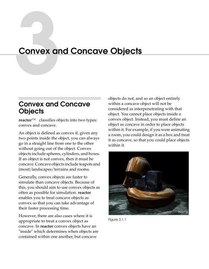
An object is defined as convex if, given any two points inside the object, you can always go in a straight line from one to the other without going out of the object. Convex objects include spheres, cylinders, and boxes. If an object is not convex, then it must be concave. Concave objects include teapots and (most) landscapes/terrains and rooms.
Generally, convex objects are faster to simulate than concave objects. Because of this, you should aim to use convex objects as often as possible for simulation. reactor enables you to treat concave objects as convex so that you can take advantage of their faster processing time.
However, there are also cases where it is appropriate to treat a convex object as concave. In reactor convex objects have an "inside" which determines when objects are contained within one another, but concave
objects do not, and so an object entirely within a concave object will not be considered as interpenetrating with that object. You cannot place objects inside a convex object. Instead, you must define an object as concave in order to place objects within it. For example, if you were animating a room, you could design it as a box and treat it as concave, so that you could place objects within it.
Figure 3.1.1

Chapter 3: Convex and Concave Objects14
About This TutorialThis tutorial describes the difference between convex and concave simulation geometries in reactor. This tutorial also describes how to group objects together to create a compound rigid body. When you complete this tutorial, you will be able to:
• Perform a convexity test.
• Treat an object as convex.
• Treat an object as concave.
• Build a compound rigid body.
Performing a Convexity TestIf you are unsure whether an object is convex or concave, you can perform a convexity test. reactor enables you to select an object and check its geometry.
To perform a convexity test:
1. Open the Utilities command panel.
2. Expand the Properties rollout from the reactor utility.
3. Select the object you want to test from any of the view panes.
4. Click the Test Convexity button.
5. A dialog box containing the result of the test is then displayed.
Treating an Object as ConvexFor the purposes of simulation, reactor must define the simulation geometry of a body, which may differ from its display geometry. The most important factor that determines this is whether the object should be considered as convex or concave. Generally, convex objects faster to simulate than concave objects, so it makes sense to treat objects as convex where possible.
reactor enables you to treat an object as convex in five different ways. You can:
• Surround the object with an invisible box (Figure 3.4.1)
• Surround the object with an invisible sphere (3.4.2)
• Surround the object with invisible wrapping (3.4.3)
Figure 3.4.1

Treating an Object as Convex 15
Figure 3.4.2
Figure 3.4.3
Figure 3.4.4
• Substitute the geometry of the object with that of a different convex object (Figure 3.4.4). It makes sense to re-use geometries through substitution because it considerably reduces file size. This is especially useful if you are repeating the same geometry several times in a scene
• Substitute the geometry of the object with an optimized version of the geometry of the object. Optimization is the process of reducing the complexity (the number of vertices) of a simulated geometry. The display remains the same.
The figures above show the actual simulation geometry in each of four cases, using the Sim Edges display option under the Geometry menu in the preview window.
In this tutorial, create a scene with a rigid body collection containing a number of simple concave and convex objects. Then follow these steps:
1. Expand the Properties rollout from the reactor utility.
2. Select an object from any of the view panes.
3. In the Properties rollout select one of the options from the convex section (Figure 3.4.5). The five possibilities are detailed below.
Figure 3.4.5

Chapter 3: Convex and Concave Objects16
Bounding Box Select the Use Bounding Box option. This uses the tightest world-axis-aligned box.
Bounding Sphere Select the Use Bounding Sphere option. This uses the tightest bounding sphere.
Convex Hull Select the Use Mesh Convex Hull option. This simulation uses the convex hull of this object, which is different from the original if the object is concave.
Substituting the GeometrySelect the Use Proxy Convex Hull option, and select any object from any of the view panes. This substitutes the geometry and the name of the proxy object is displayed on the button below the Use Proxy Convex Hull option.
Substitute for Optimization Select the Use Optimized Convex Hull option, and use the Min/Max bar to set the appropriate level of optimization. reactor then optimizes the object before every simulation.
By running the simulation and selecting Sim Edges from the Geometry menu, you can view the geometries that are physically simulated for the objects. In this way you can always see how accurately your simulation geometry conforms to the display geometry, and hence how likely you are to see any visual disparities between simulation and
display in both the preview window and in creating a 3ds max animation. Accurate simulation geometry yields more accurate (but slower) simulation.
Treating an Object as ConcaveMany objects you create are concave and cannot be accurately modeled during simulation by substituting them with convex simulation geometries. Also, concave objects can contain other objects, whereas convex objects cannot. So if you are using a box to represent a room, you must treat the box as concave in order to place objects within it. In addition, 3ds max planes must be treated as concave.
You can treat an object as concave by using its original mesh. This mesh can be concave. In addition, you can substitute the geometry of an object with that of a nearby concave or convex object, which is considered as being hollow. As with convex objects, you can also substitute an object with a system-generated, optimized version of the object.
Using the Original Object MeshTo create a box and a number of smaller objects to go into the box, follow these steps:
1. Create a scene with a rigid body collection containing a box called Box01 and a number of smaller objects that could fit into the box.
2. Open the Utilities command panel.
3. Expand the Properties rollout (Figure 3.5.1).
4. Select the object called Box01 from any of the view panes.

Building a Compound Rigid Body 17
5. Select the Use Mesh option from the Concave properties rollout.
Figure 3.5.1
reactor now treats the object as concave.
Substituting the Geometry of an Object with a Proxy MeshUsing the same box and smaller objects from the pervious example, you can use a proxy mesh to treat the box as convex, as follows:
1. Open the Utilities command panel.
2. Select the Use Proxy Mesh option.
3. Select one of the concave objects in the scene.
The geometry is substituted and the name of the concave object displays on the button below the Use Proxy Mesh button.
Substituting the Geometry of an Object with an Optimized MeshYou can use an optimized mesh to treat the box as convex, as follows:
1. Open the Utilities command panel.
2. Select the Use Optimized Mesh option.
3. Use the Min/Max bar to set the appropriate level of optimization.
reactor now optimizes the object before every simulation.
You can treat any convex geometry as a concave one. This results in slower simulation, but such objects can hold other objects. The likely places for using concave objects are for solid bodies that need more accurate simulation, or for bodies that have no volume - such as planes or meshes that are not closed.
Building a Compound Rigid Bodyreactor can join several meshes together to create a more complex body. Rigid bodies in reactor are usually composed of one or more primitives. Primitives are the basic elements that make up objects. Primitives can be planar, spherical, or geometric. Rigid bodies composed of more than one primitive are called compound rigid bodies.
Rigid bodies have elasticity and friction. Primitives each have mass, whose sum determines the mass of the compound body.
Compound rigid bodies are useful if you want to simulate an object with uneven density, or a concave object that can be decomposed into several convex segments. Compound objects provide an interim between convex and concave bodies, in that they are faster to simulate than concave objects and allow you to do things like place objects within them. However, they are less accurate in simulation than true concave objects.
You build compound rigid bodies using the Group function within 3ds max. For more information on groups, see the 3ds max documentation.
Chapter 3: Convex and Concave Objects18
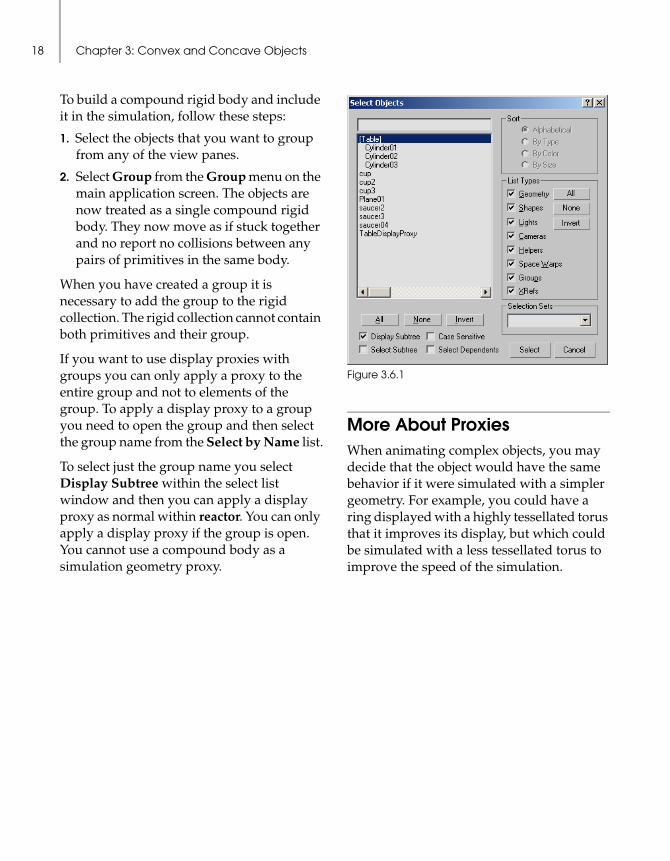
To build a compound rigid body and include it in the simulation, follow these steps:
1. Select the objects that you want to group from any of the view panes.
2. Select Group from the Group menu on the main application screen. The objects are now treated as a single compound rigid body. They now move as if stuck together and no report no collisions between any pairs of primitives in the same body.
When you have created a group it is necessary to add the group to the rigid collection. The rigid collection cannot contain both primitives and their group.
If you want to use display proxies with groups you can only apply a proxy to the entire group and not to elements of the group. To apply a display proxy to a group you need to open the group and then select the group name from the Select by Name list.
To select just the group name you select Display Subtree within the select list window and then you can apply a display proxy as normal within reactor. You can only apply a display proxy if the group is open. You cannot use a compound body as a simulation geometry proxy.
Figure 3.6.1
More About ProxiesWhen animating complex objects, you may decide that the object would have the same behavior if it were simulated with a simpler geometry. For example, you could have a ring displayed with a highly tessellated torus that it improves its display, but which could be simulated with a less tessellated torus to improve the speed of the simulation.

More About Proxies 19
Geometry ProxiesGeometry proxies allow you to use a different geometry for the simulation that the one you are actually going to animate and display in 3ds max. Select the Use Proxy Convex Hull option if you want to use another object's convex hull, or Use Proxy Mesh if you want to use the mesh of another concave object.
There are several cases where you might want to use proxy geometries: While you probably want to animate and display a highly tessellated torus, you want the simulation and the preview in window to be fast. Substituting the simulation geometry of the torus for a simpler one allows you to do that. (Figure 3.7.1)
Figure 3.7.1
Figure 3.7.2
You might also use the same geometry in many places. Using the same proxy geometry for each object creates only one instance of geometry, which is shared by all objects during simulation. This helps to reduce the amount of information exported, the loading a creation of the scene, and the amount of memory used.
Primitives use proxy geometries, which means that you can define different proxy geometries for the primitives inside a compound rigid body, but not for the compound body itself.
Optimized Geometriesreactor can automatically create proxy geometries. In fact, when you choose Use Bounding Box, or Use Bounding Sphere what you are actually creating is a simple proxy geometry. The Use Optimized Convex Hull and Use Optimized Mesh options automatically create an optimized version of your geometry and use it as a proxy. They internally apply the Optimize modifier to the mesh. However, it is recommended that you create you own optimized geometries if you want full control over the results.
Chapter 3: Convex and Concave Objects20
Display ProxiesDisplay proxies substitute the actual rigid bodies when they are displayed at run-time. They are mainly useful for real-time application developers who want to preview and export display information.
If you select a display proxy for a rigid body, the rigid body display is substituted by the display of the chosen node and its children during the reactor run-time simulation. That means you can simulate quite a simple body but display a very complex object. This is similar to what you can do with geometry proxies, but there are important differences:
1. While geometry proxies apply to primitives, display proxies apply to rigid bodies
2. When you are creating an animation in 3ds max, the animated bodies are the ones added to the simulation. Display proxies don't play any role in creating 3ds max animations, since they are only used for real-time display.
Another important reason (for real-time developers) for using display proxies is similar to the one explained in the previous point about geometry proxies. If you are displaying the same object in many places, you should use display proxies that point to the same object so the display object will only be created/exported once with the subsequent saving in time and memory.
Other Alternatives for AnimatorsWhile geometry proxies and display proxies are very useful and powerful, there are other alternatives for animating a given body using a different one in a simulation.
You can create both the simple and complex object, set the properties on the simple object and add it to the simulation. Perform the simulation, and once it is finished, you can match the positions of the simple and complex objects, and then link the complex object to the simple one. The complex object will follow the same animation of the simple one. In this case, you should not render the simple object when rendering.
Useful HintsIf you check the Geometry / Sim Edges option in the preview window you will be able to see the geometries that are actually being used in the simulation.
Soft BodiesA soft body is a body whose geometry deforms due to physical interactions. They can bend, flex, stretch and other similar movements. Soft bodies have a wide number of uses, but they can be more demanding and slow a real-time simulation down.
As with rigid bodies, soft bodies operate through collections. These are called soft body collections. Soft body collections perform the same functions as rigid body collections.
Soft body have a greater range of physical properties to properly describe their motion than rigid bodies. These include properties such as damping, smoothing and stiffness. The properties are applicable to soft bodies in addition to the rigid properties of mass and friction.
Most soft bodies that you create using 3ds max™ use a rigid body as their initial starting point. You normally create a soft body by first creating the rigid shape of the
body and then turning it into a soft body. There are two ways of defining a soft body in reactor™ , depending on whether you use the FFD modifier.
As in previous chapters, the bulk of this chapter consists of two tutorials that will guide you through the two possible processes of soft body creation.
About These TutorialsThere are two tutorials in this chapter. The first tutorial introduces reactor soft bodies to users. It describes how to use reactor to create a simple scene with soft bodies. It also describes the effects generated by varying the parameters for soft bodies. When you complete this tutorial, you will be able to:
• Create a soft body collection.
• Add objects to the soft body collection.
• Assign physical properties to soft objects in a scene.
Chapter 4: Soft Bodies22
In the Scenes folder in the reactor directory, there are two files associated with this tutorial. They show how your scene should appear at the start and at the end of the tutorial. They are called TutorialTwoStart.max and TutorialTwoEnd.max.
Creating a Soft Body SimulationWhen creating a simulation that contains soft bodies, you use techniques similar to rigid body simulation. You create the objects in 3ds max. For objects that are soft you apply a Soft modifier and include them in a soft body collection. You add this soft body collection to the simulation in the same way as a rigid body collection.
You should take care not to include the objects in both the rigid and soft collections. When you apply a modifier to a rigid object to make them soft, its rigid equivalent still exists in the scene.
Simple Soft Body CreationYou can follow these steps to create the tutorial soft body:
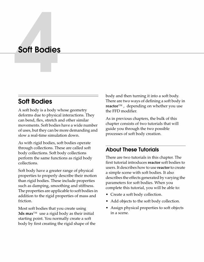
1. Create a scene as detailed in Figure 4.2.1. To create a star, choose star from the shapes menu and then apply the extrude modifier. You should also create three standard planes rotated to roughly 30, 0 and -30 degrees. If you don't want to create the scene you can load TutorialTwoStart.max
2. Select a concave mesh for each of the planes in the Properties rollout from the reactor utility. Standard 3ds max planes require a concave simulation geometry.
Change their friction to 0.9 so our star rolls instead of sliding.
3. Add a rigid body collection to your scene.
4. Add the planes to the rigid body collection.
5. Select the star, expand the Modify section and select reactor SoftBody from the drop-down list.
Figure 4.2.1
Soft Body PropertiesIn the Properties rollout for the SoftBody modifier you can set physical attributes for objects. There are four main options for the physical properties of a soft body.
Mass
This mass applies to the soft body. Though you may have applied a mass in the Properties section from the reactor Utility, the soft body won't have the correct mass unless it is applied here.
More Advanced Soft Bodies 23
Stiffness
Changing this value changes the stiffness of the body. Valid values are between 0 and 1000, where 1000 relates to the stiffest value. The default value is 0.2. If you set a value over than 1, reactor applies the default value.
Damping
This is the damping coefficient for the oscillation of the body's compression and expansion, with values are between 0 and 1, where 1 provides the greatest damping.
Friction
This is the coefficient of friction for the body's surface, similar to the corresponding coefficient for rigid bodies.
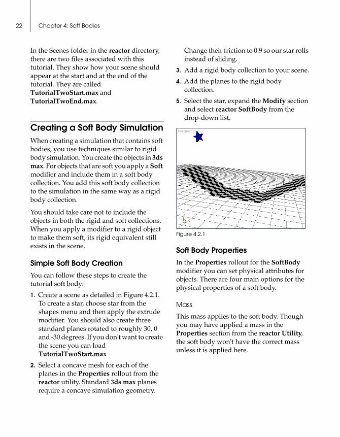
Creating and Adding Bodies to a Soft CollectionYou must add your soft body to a soft body collection. The button for a soft body collection is in the Create panel, in the Helpers option. It is a reactor option.
Follow these steps to assign the tutorial soft body to a collection:
1. Select the reactor drop-down menu, and click the SBCollection button.
2. Select the collection symbol.
3. Open the Modify tab and click Add or Pick to select the soft bodies from the available list.
4. Click the Preview in Window button and reactor displays your scene.
When you pick up a soft body with the mouse, it flexes. This is due to the fact that the mouse actually connects a spring between the nearest vertex and the mouse pointer. The strength of the spring can be adjusted.
Figure 4.2.2
More Advanced Soft BodiesSoft Bodies require accurate simulation. As a result, you may find that you need to set the accuracy level of the simulation much higher than that needed for rigid bodies. The best way to customize this is by using the Scale
Chapter 4: Soft Bodies24
Timestep parameter in the Advanced rollout of the soft collection containing the bodies. Typically, fewer vertices in a soft body result in faster physical calculation.
You can have smooth soft bodies. Certain techniques, such as applying the Mesh Smooth modifier from 3ds max after the Soft Body modifier are sometimes preferable to simply increasing the number of vertices in a body. For animation, the accuracy can be improved by increasing the number of substeps per keyframe. You can also improve display simulations in the preview window by reducing the size of the timestep or increasing the number of substeps per timestep.
Fixing Soft ObjectsTo fix certain points in objects to world space, you need to apply the Soft Body modifier to a subset of the object's vertices instead of to the entire body. You can use the Mesh Select modifier in 3ds max to select vertices, before you apply the Soft Body modifier. You select the points in the object that you want fixed, invert the selection and when applying the soft body modifier, you check the Non-Selected are Fixed option.
SmoothingWithin the Soft Body modifier is an option called Smooth Level that allows you to apply iterative subdivisions to the mesh, which is a useful tool to add a smoother appearance to the soft body. There are three levels from 0 to 2 iterations of subdivision. This subdivision is only applicable in real-time simulation. It is useless for animation. You should apply this modifier before applying the reactor Soft Body modifier.
Disabling Collections You can temporarily remove an entire soft body collection from simulation by checking this box.
Advanced Soft Collection OptionsThe Modify panel for a soft body collection has an Advanced rollout. Unlike rigid bodies, you cannot change the energy threshold for soft bodies, as soft bodies cannot be deactivated. You also cannot ignore collisions between soft bodies in a soft body collection.
The Scale Timestep parameter changes the internal integration step of the soft collection. If the soft body is behaving in an unstable or unrealistic manner, you can set this parameter to less than 1 to force the collection to take a proportionally smaller timestep. You can achieve faster simulation by increasing this parameter. The integrator then integrates at a higher than the default timestep. However, there is a risk of instability in doing this.
Freeform DeformationOne of the better tools that you can use in reactor for soft bodies is the FFD (Freeform Deformation) tool. The FFD tool lets you encase a soft body in a simple mesh, and use the mesh for calculating the physics of the body. Using this tool, it becomes much easier to deform soft bodies, and less expensive on system resources. The trade-off with FFD soft bodies is that they are less accurately modeled than other soft bodies.
Freeform Deformation 25
This second tutorial covers FFD soft bodies. When you complete this tutorial, you will be able to create an FFD soft body.
In the Scenes folder in the reactor directory, there are two files associated with this tutorial. They show how your scene should appear at the start and at the end of the tutorial. They are TutorialThreeStart.max and TutorialThreeEnd.max.
Creating an FFD Soft BodyThis tutorial shows you how to create a soft body that uses freeform deformation.
1. Create a teapot above a plane mesh. Add the plane to a rigid body collection. You can load the scene directly from TutorialThreeStart.max
2. Select the teapot and, under the Modify panel, select FFD (box) from the drop-down list.
3. From the modifiers select reactor SoftBody.
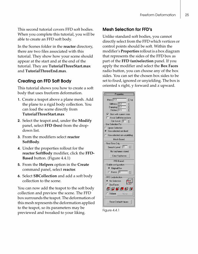
4. Under the properties rollout for the reactor SoftBody modifier, click the FFD-Based button. (Figure 4.4.1)
5. From the Helpers option in the Create command panel, select reactor.
6. Select SBCollection and add a soft body collection to the scene.
You can now add the teapot to the soft body collection and preview the scene. The FFD box surrounds the teapot. The deformation of this mesh represents the deformation applied to the teapot, so its parameters may be previewed and tweaked to your liking.
Mesh Selection for FFD'sUnlike standard soft bodies, you cannot directly select from the FFD which vertices or control points should be soft. Within the modifier's Properties rollout is a box diagram that represents the sides of the FFD box as part of the FFD (un)selection panel. If you apply the modifier and select the Box Faces radio button, you can choose any of the box sides. You can set the chosen box sides to be set to fixed, ignored or unyielding. The box is oriented x right, y forward and z upward.
Figure 4.4.1
Chapter 4: Soft Bodies26
Another method of selection is using the Volume button. You can create another volume that intersects the FFD's volume. Then, you select the Volume button and choose this second volume as your de-selecting volume. This results in the None button acquiring the name of your new volume, and all the point of the FFD mesh that coincide with the new volume becoming de-selected.
You can also change the original FFD configuration. You might wish to do this to get a better fit between the FFD and the underlying geometry. This gives you more accurate collision detection with the geometry, and a more accurate simulation.
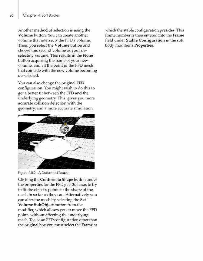
Figure 4.5.2 - A Deformed Teapot
Clicking the Conform to Shape button under the properties for the FFD gets 3ds max to try to fit the object's points to the shape of the mesh in so far as they can. Alternatively you can alter the mesh by selecting the Set Volume SubObject button from the modifier, which allows you to move the FFD points without affecting the underlying mesh. To use an FFD configuration other than the original box you must select the Frame at
which the stable configuration presides. This frame number is then entered into the Frame field under Stable Configuration in the soft body modifier's Properties.

Clothreactor™ can physically model and simulate cloth. A cloth may appear to be a soft body, but there are some major differences. The principal difference between a soft body and a cloth is that soft bodies are three-dimensional, whereas cloths are two-dimensional.
A cloth is composed of a mesh of triangles that have physical properties. You can use them to simulate clothes, trampolines, sheets of metal and other two-dimensional items. Theoretically, you could use soft bodies for some of these purposes, but a cloth is much more practical because there is no need to simulate a negligible volume.
As with other body types, cloth bodies need to belong to an entity collection in order to function properly. Cloths use cloth collections .
Cloths have physical properties similar to other bodies. They also have some values specific to themselves, such as buoyancy, which are necessary to compensate for their two-dimensional nature.
About This TutorialYou can create cloth objects using the modifier reactor Cloth. In this tutorial you will create a table, an object on the table and a cloth above it. The cloth drops onto the table and the object. By the end of the tutorial you will be able to:
• Create a cloth and cloth collection.
• Add objects to a cloth collection.
• Assign physical properties to cloths in a scene.
In the Scenes folder in the reactor directory, there are two files associated with this tutorial. They show how your scene should appear at the start and at the end of the tutorial. They are TutorialFourStart.max and TutorialFourEnd.max
Chapter 5: Cloth28
Creating a Cloth SimulationTo change an object in 3ds max™ to a cloth, you apply a modifier to it and the object's mesh is used to define a two dimensional cloth.
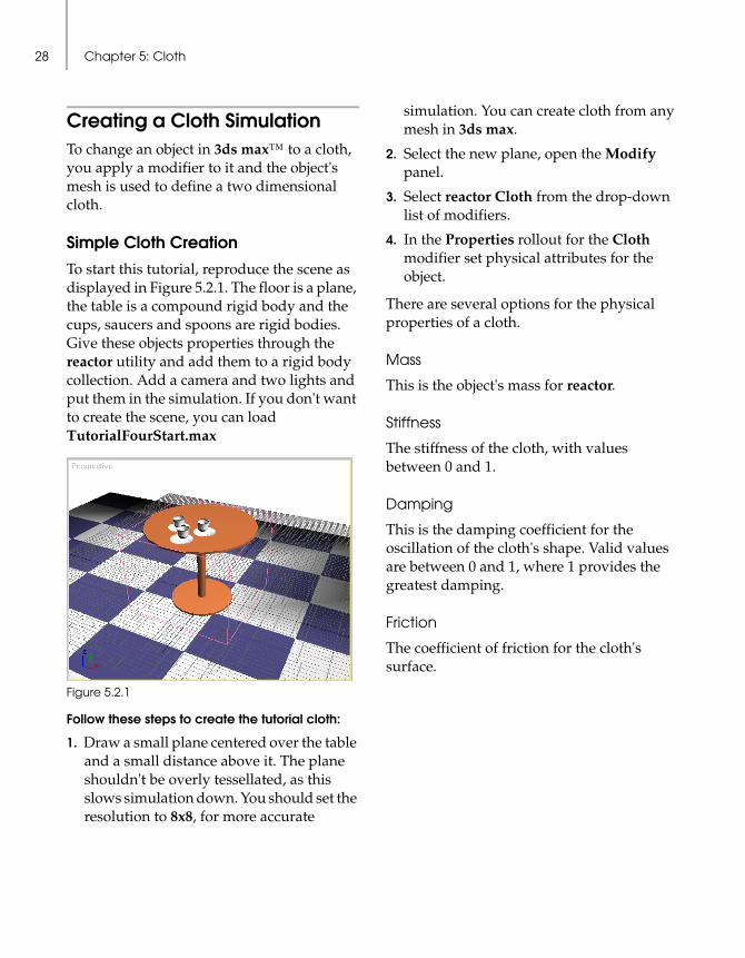
Simple Cloth CreationTo start this tutorial, reproduce the scene as displayed in Figure 5.2.1. The floor is a plane, the table is a compound rigid body and the cups, saucers and spoons are rigid bodies. Give these objects properties through the reactor utility and add them to a rigid body collection. Add a camera and two lights and put them in the simulation. If you don't want to create the scene, you can load TutorialFourStart.max
Figure 5.2.1
Follow these steps to create the tutorial cloth:
1. Draw a small plane centered over the table and a small distance above it. The plane shouldn't be overly tessellated, as this slows simulation down. You should set the resolution to 8x8, for more accurate
simulation. You can create cloth from any mesh in 3ds max.
2. Select the new plane, open the Modify panel.
3. Select reactor Cloth from the drop-down list of modifiers.
4. In the Properties rollout for the Cloth modifier set physical attributes for the object.
There are several options for the physical properties of a cloth.
Mass
This is the object's mass for reactor.
Stiffness
The stiffness of the cloth, with values between 0 and 1.
Damping
This is the damping coefficient for the oscillation of the cloth's shape. Valid values are between 0 and 1, where 1 provides the greatest damping.
Friction
The coefficient of friction for the cloth's surface.

Creating a Cloth Simulation 29
Rel Density
As cloth has no volume, a density for the cloth cannot be calculated. So there is a buoyancy property for cloths, which reflects its relative density. Its default value is 1, the density of water.
Figure 5.2.2
Intersection
You can set a cloth not to intersect with itself by checking Avoid Self-Intersections.
Deformation
You can apply a level of deformation constraint using Constrain Deformation. The deformation constraint percentage represents how much the cloth can stretch. A low value means it hardly stretches.
Vertex Selection
Allows certain points of the cloth to be fixed in world space. You can apply this modifier to the entire body, or a selection of the body's vertices. Depending on the selection, you can select options such as Non-selected Are Fixed to fix the position of certain features in world space.
Smooth Level
Applies iterative subdivision during real time simulation.
Air Resistance
This is the damping coefficient for the oscillation of the rope's compression and expansion. Valid values are between 0 and 1, where 1 provides the greatest damping.
Adding Bodies to a Cloth CollectionYou can create a cloth collection in much the same way as any other type of entity collection. To add a cloth collection, you open reactor. Then you click the CLCollection button and add a collection to the scene. To add cloths to the collection select the collection and click Add or Pick.
Chapter 5: Cloth30
Click the Preview in Window button and reactor displays your scene. Cloth collection optimization is similar to soft body collection optimization.
High levels of smoothing may lead to apparent intersections of the cloth and other objects. These are not actually there in the simulation, which accurately simulates the underlying mesh. Using the on Avoid Self-Intersections option results in more accurate simulation of the cloth at the cost of an increased simulation time. For a large mesh this can be very slow.
Advanced Cloth PropertiesIn the Properties section for cloth are several additional properties that you can use to better define the physics of your cloths.
Force ModelsThere are two kinds of force model: Simple and Complex. Each allows you to model the forces that affect a cloth in different ways, with the trade between the two options being one of system resources. Complex forces are more accurate, but more expensive to use and therefore sometimes unsuitable to your needs.
Simple Force Model
The simple model is fine for most situations. Stiffness determines the stiffness of the cloth, incorporating both stretch and shear stiffness properties.
Complex Force Model
This is a more accurate model of cloth dynamics, which incorporates independently adjustable stretch and shear properties, as well as a physically accurate out-of-plane bend property.
The damping parameters in both models control how quickly the cloth dissipates energy as it changes shape. There is no correlation between the meaning of a value in one model and any value in the other model. A stiffness of .2 in the simple force model does not correspond to stiffness of .2 in the complex model, in terms of cloth behavior.
Fold StiffnessFold stiffness provides you with an additional method for adding stiffness to a cloth. It also controls the degree to which a cloth is able to bend, which in turn affects how it folds. Cloth behaves like loose materials such as silk by default. Fold stiffness allows you to simulate stiffer materials such as wool or linen. With high degrees of fold stiffness, you can even simulate sheet metal.
There are two types of fold stiffness: Simple Fold Stiffness and Complex Fold Stiffness.
Limitations of the Cloth Model 31
Simple Fold Stiffness
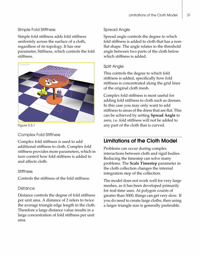
Simple fold stiffness adds fold stiffness uniformly across the surface of a cloth, regardless of its topology. It has one parameter, Stiffness, which controls the fold stiffness.
Figure 5.3.1
Complex Fold Stiffness
Complex fold stiffness is used to add additional stiffness to cloth. Complex fold stiffness provides more parameters, which in turn control how fold stiffness is added to and affects cloth.
Stiffness
Controls the stiffness of the fold stiffness.
Distance
Distance controls the degree of fold stiffness per unit area. A distance of 2 refers to twice the average triangle edge length in the cloth. Therefore a large distance value results in a large concentration of fold stiffness per unit area.
Spread Angle
Spread angle controls the degree to which fold stiffness is added to cloth that has a non-flat shape. The angle relates to the threshold angle between two parts of the cloth below which stiffness is added.
Split Angle
This controls the degree to which fold stiffness is added, specifically how fold stiffness is concentrated along the grid lines of the original cloth mesh.
Complex fold stiffness is most useful for adding fold stiffness to cloth such as dresses. In this case you may only want to add stiffness to areas of the dress that are flat. This can be achieved by setting Spread Angle to zero, i.e. fold stiffness will not be added to any part of the cloth that is curved.
Limitations of the Cloth ModelProblems can occur during complex interactions between cloth and rigid bodies. Reducing the timestep can solve many problems. The Scale Timestep parameter in the cloth collection changes the internal integration step of the collection.
The model does not work well for very large meshes, as it has been developed primarily for real-time uses. At polygon counts of greater than 3000, things can get very slow. If you do need to create large cloths, then using a larger triangle size is generally preferable.

Chapter 5: Cloth32
Figure 5.3.2
Constrain Deformation can cause heavy system usage in some situations, especially when the cloth stiffness is low. It can cause cloth-to-cloth and cloth-to-rigid body interactions to behave less effectively.
It is important to know that you can create cloth from any mesh in 3ds max. Although a square grid based triangulation may be the default for many meshes, this can result in visual artifacts during cloth simulation, particularly due to collinear creasing. It is advisable to try and use a more irregular triangulation of the mesh, such as the Delaunay triangulation of a 3ds max Nurbs surface. (To obtain this triangulation, select the Surface Approximation rollout in the Nurbs modifier panel. Select Advanced Parameters, and check the Delaunay check box in the Advanced Surface Approximation dialog.)
Using Update MaxUsually in a scene you do not want your cloth to start off in an animation as a flat plane or as its original configuration. For example, you might want it to drape around a body. To achieve this, you can use the Update Max function from the Preview window.
Create a scene with cloth and preview it. Within the Preview window, position the cloth as you would like it to be at the start of your animation and then select Update Max from the Max menu in the window. When you return to 3ds max the scene will have updated to represent the changes you made in the Preview window.
This is very useful for getting curtains to hang in folds, or for getting a dress to hang properly around a body from the start of an animation.
RopeYou can create ropes using any of the objects from the Shapes tab within 3ds max. As with other object types in the system, ropes operate in entity collections. They are called rope collections. They perform the same functions as rigid body collections.
Most ropes that you create use a spline. You normally create a rope by first creating a spline and then turning it into a rope by applying a modifier. There are two ways of simulating rope in reactor™ , depending on whether you wish to use a spring or constraint based model.
This chapter consists of one tutorial that guides you through making a rope in a scene.
About These TutorialsThere is one tutorial in this chapter. It describes the creation of a rope with a fixed end and a free end. It also describes the effects you can achieve by varying the parameters for the rope. When you complete this tutorial, you will be able to:
• Create a rope collection.
• Add objects to the rope collection.
• Assign physical properties to ropes in a scene.
In the Scenes folder in the reactor directory, there are two files associated with this tutorial. They show how your scene should appear at the start and at the end of the tutorial. They are called TutorialfouraStart.max and TutorialfourbEnd.max.
Creating a Rope SimulationWhen creating a simulation that contains ropes, you use techniques similar to soft body simulation. You create the splines in 3ds max, and apply a Rope modifier. You also include them in a rope collection.
You should take care not to include the objects in both the rigid and soft collections. When you apply a rope modifier to an object, its rigid equivalent still exists in the scene.
Chapter 6: Rope34
Simple Rope CreationThe following steps create the tutorial scene:
1. Create a scene as detailed in Figure 6.2.1. To create the helix, select Helix Shape from the Shapes tab. Add the sphere a small distance below the helix so that if the helix was fully relaxed it would reach the plane.
2. Select Use Bounding Sphere for the sphere in the Properties rollout from the reactor utility, as described in the previous section.
3. Add a rigid body collection to your scene.
4. Add the plane to the rigid body collection (but do not add the helix) .
5. Select the helix, expand the Modify rollout, and select Normalize Spline. This splits the spline into segments of equal length. Within this modifier set the segment length to between 5 and 10.
6. Select Spline Select from the list of modifiers. By default, Spline Select selects vertices. This suits our purpose in this case. Select all of the vertices from the helix except the center one.
7. Apply the reactor Rope modifier from the list of modifiers.
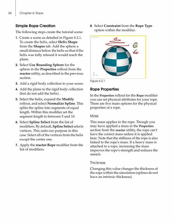
8. Select Constraint from the Rope Type option within the modifier.
Figure 6.2.1
Rope PropertiesIn the Properties rollout for the Rope modifier you can set physical attributes for your rope. There are five main options for the physical properties of a rope.
Mass
This mass applies to the rope. Though you may have applied a mass in the Properties section from the reactor utility, the rope can't have the correct mass unless it is applied here. Note that the stiffness of the rope is also linked to the rope's mass. If a heavy mass is attached to a rope, increasing the mass improves the rope's strength and reduces the stretch.
Thickness
Changing this value changes the thickness of the rope within the simulation (splines do not have an intrinsic thickness).

Creating a Rope Simulation 35
Air Resistance
This is the damping coefficient for the oscillation of the rope's compression and expansion. Valid values are between 0 and 1, where 1 provides the greatest damping.
Friction
This is the coefficient of friction for the rope's surface, similar to the corresponding coefficient for rigid bodies.
Rope Type
This defines the type of rope model used for simulation. Either spring or constraint may be used. When minimizing stretch it is advisable to use the constraint model.
Figure 6.2.2
Creating and Adding Ropes to a Rope CollectionWhen you have created a rope, you must add it to a rope collection. The button for a rope collection is in the Create menu, in the Helpers option. You can follow these steps to assign the tutorial rope to a collection.
1. Select the reactor drop-down menu, and click the RPCollection button.
2. Select the collection symbol, open the Modify tab, click Add and select the ropes from the available list. You can also click Pick and select the bodies manually from the view-panes.
3. If you have added a camera, ensure that it has been positioned correctly and any lights you might require have also been added.
4. Click the Preview in Window button and reactor displays your scene.
When you pick up a rope with the mouse it flexes. This is due to the fact that the mouse actually connects a spring between the nearest vertex and the mouse pointer.
Note: In order for wind and water to affect rope you need to specify the rope's thickness value as greater than 0. This provides a surface area that the forces which wind and water apply can affect. The thicker the rope the greater the surface area. The greater the effect the wind has, the larger the ripples and greater the buoyancy for water interaction.
Note: can avoid self intersections in a manner much the same as cloth. However, there is one important difference. You must set the thickness of the rope to a value greater than zero. Otherwise, you may get results wherein the rope may appear to self intersect. This is because a rope with zero thickness has no effect on whether it’s display shell intersects. The 3ds max spline display thickness does not affect the reactor rope thickness, so simply changing the display’s thickness would not solve this problem.

Chapter 6: Rope36

WaterWater is the reactor representation of bodies of fluids that you can use to enhance a scene. Objects can interact with water in physically realistic ways, including ripples and waves. Water can also have different densities, which is a crucial factor in determining whether an object floats or sinks. The buoyancy properties for objects other than cloth are calculated automatically from the shape and mass properties for the objects.
Water in reactor™ is a space warp that is simulated as water when brought into the display simulation. Since you cannot render space warps, you must provide water with a graphical representation. In preview mode, you can see a representation, but in a proper simulation, water does not appear. You can give water a graphical representation by binding a plane to the water space warp. In fact, you can bind the warp to any sort of object.
About This TutorialIn this tutorial you will learn to use reactor Water. By the end of this tutorial you should be able to:
• Add water to a scene.
• Set properties for the water.
• Bind the water to a non-physically simulated element in the scene.
In the Scenes folder in the reactor directory, there are two files associated with this tutorial. They show how your scene should appear at the start and at the end of the tutorial. They are called TutorialFiveStart.max and TutorialFiveEnd.max.
Chapter 7: Water38
Figure 7.21
Adding Water to a Scene
Using Water in a Simple SimulationReproduce the scene as shown in Figure 7.2.1. There are five fixed boxes with zero mass, which act as a pool, a camera and two lights. Create the rigid collection for the boxes.
Figure 7.2.2
If you don't want to create the scene, you can load TutorialFiveStart.max.
To add water to the pool, use the following instructions.
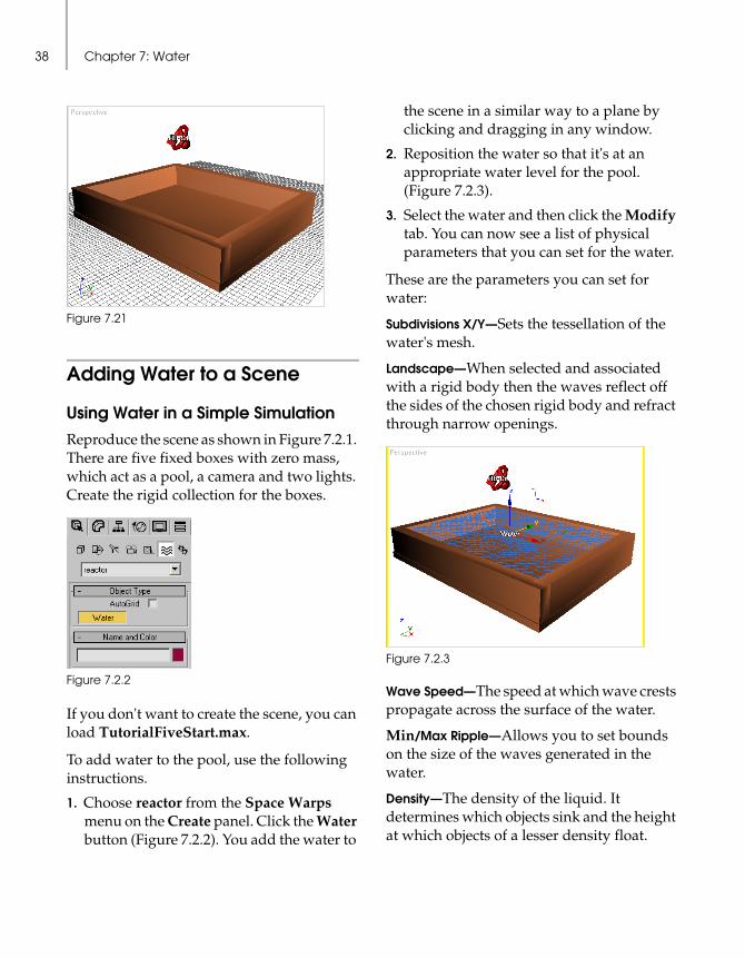
1. Choose reactor from the Space Warps menu on the Create panel. Click the Water button (Figure 7.2.2). You add the water to
the scene in a similar way to a plane by clicking and dragging in any window.
2. Reposition the water so that it's at an appropriate water level for the pool. (Figure 7.2.3).
3. Select the water and then click the Modify tab. You can now see a list of physical parameters that you can set for the water.
These are the parameters you can set for water:
Subdivisions X/Y—Sets the tessellation of the water's mesh.
Landscape—When selected and associated with a rigid body then the waves reflect off the sides of the chosen rigid body and refract through narrow openings.
Figure 7.2.3
Wave Speed—The speed at which wave crests propagate across the surface of the water.
Min/Max Ripple—Allows you to set bounds on the size of the waves generated in the water.
Density—The density of the liquid. It determines which objects sink and the height at which objects of a lesser density float.

Adding Water to a Scene 39
Viscosity—This is a measure of resistance to flow and thus how difficult it is for objects to move through the liquid. A larger value means that the motion of objects through the water is highly damped.
Water in MotionIf you click the Preview in Window button, you can able to see the water in the pool. The next step is to add some objects that you can drop into the water and see how they react to the water and how it reacts to them.
Figure 7.2.4
Add two boxes above the water and give them a mass. Note that this mass should be large enough to make the objects slightly less dense than water (density of water is 1000kg/m3). Add them to the collection and preview the simulation again. When you play the simulation, the boxes fall into the water and bob around. Try dragging the boxes under the water and letting them go. You can try adding a strange shape into the water. If you drag it through the water, it reorients to the path of least resistance. For example, if you try dragging a stick through the water edge on, it reorients so that its tip
points in the direction of motion. Note that objects may deactivate during simulation if they have a deactivator, even if they're still in the water.
Animating Water for 3ds maxThe next step is to provide a representation for 3ds max so that you can render the scene for pictures or animations. Draw a plane of the same size as the water and in the same position and orientation. Select the Bind to Space Warp icon from the Main toolbar, click the plane and drag to the water. When you render it, you should see your plane. You can apply materials to the plane and it renders as such.
Binding a plane to the water applies a modifier to the plane within which you can set the scale strength for the deformation. For example, if you set the scale strength to 2, then any water deformation is doubled for the plane.
If you make an animation with the water, the plane mimics the water's behavior and you can render the animation.
Figure 7.2.5

Chapter 7: Water40

ConstraintsSuppose that you create a scene in which you want to tightly control the movement of physical objects. Perhaps you want to make two objects constantly spring together, or have one object hinged onto another. To achieve these kinds of motion restriction, you use constraints.
Constraints limit the behavior of objects, fixing them to points in space, or objects. There are a number of constraint systems in reactor™ . The most robust are point-to-point, point-to-path and point-to-nail constraints. There are also two basic types of constraint called springs and dashpots. Springs and dashpots tend to be faster, but more elastic in nature.
A spring is an elastic connection between two objects. A dashpot is similar, but more flexible. It allows for elastic connection of two objects with a point, or an object with a point in space. Dashpots can also constrain the position and orientation of objects.
The final section of this chapter describes the reactor toy car object, which is built from various types of constraint. It is meant only as something with which to play. It is too simple for simulating a real car model, but may be useful as a quick way of getting a car-like model up and running.
About This TutorialThe first part of this tutorial covers the full implementation of a spring. The second part discusses the implementation of a dashpot. The remaining constraints (simply called "constraints") are described in detail on page 45.
When you complete this tutorial, you will be able to:
• Distinguish between springs and dashpots
• Add a spring
• Change the properties of a spring
• Add a dashpot
• Change the properties of a dashpot

Chapter 8: Constraints42
In the Scenes folder in the reactor directory, there are two files associated with the spring tutorial. They show how your scene should appear at the start and at the end of the tutorial. They are called TutorialSixAStart.max and TutorialSixAEnd.max.
Springs and DashpotsThe spring system adds the action of a Hookean spring between any two rigid bodies. You can control and change the properties of the spring. For example, you can alter its stiffness, rest length, and damping value.
Rest length is the extent of the spring when it applies no force. A spring always works to attain its rest length. A rest length of zero ensures that the spring will always work to bring the objects together. Dashpots always have zero rest length.
Damping is the process of gradually reducing a vibrating motion. A high damping value results in a spring that oscillates very few times before returning to its rest length. A highly damped spring appears to have very little energy. A low damping value results in a spring that keeps extending and contracting around its rest length for a long time.
You can also suppress the extension or the contraction action of the spring. For example, a rubber band is an example of a spring with suppressed extension. If you disable both, the spring no longer works.
Dashpots are like springs with a very high damping value. Dashpots enable you to predict and control the motion of objects. There are two types of dashpot: linear and
angular. Linear dashpots force objects to try to share a point in space. The objects can move freely about this space, but always have this point in common. Angular dashpots force objects to attempt to keep their relative orientations. If you rotate one, the dashpot tends to reduce that rotation while also applying a turning force on the other so that their orientations are equal.
Adding a Spring to a SimulationUsing the spring system, you can add a spring between two rigid bodies. reactor also enables you to specify where the spring should be attached to each rigid body. To do this, you have to add a point to each rigid body.
Create a scene containing a rigid body collection with two spheres and a plane. The scene may be created from scratch or you can load in the file TutorialSixAStart.max.
Figure 8.3.1
1. Select the Helpers icon from the Create command panel within 3ds max.
2. Select reactor from the Helpers drop-down menu.

Adding a Spring to a Simulation 43
3. Click the Spring button in the Object Type rollout (Figure 8.3.1).
4. Select a view pane to draw a line anywhere in the scene.
5. Click the None button beside Object A in the Spring Properties rollout.
6. Select one of the spheres in a view pane. The sphere is now associated with one end of the spring. The name of the sphere is displayed on the button beside the words, Object A.
7. Repeat these steps to associate the second sphere with the Object B button.
You must select the points to which the spring should attach. You can either select an actual point or an object, in which case that object's pivot is used as the point. A point does not have to be on either of the objects in a spring. Its position is be fixed relative to the object and the spring forces are applied at that point for the object. If the precise point on each object is irrelevant, you can re-select the objects that you have identified as Object A and Object B, and use their pivots.
Figure 8.3.2
For a spring, the process for creating and using a point in reactor is:
1. Select the Helpers icon from the Create command panel within 3ds max.
2. Select Standard from the Helpers drop-down menu.
3. Click the Point button in the Object Type rollout (Figure 8.3.2).
4. Click in the view pane where you want the point.
5. Click the button labeled None beside Point A in the Spring Properties rollout and select the point or object you want to associate with Object A in any of the view panes.
6. Repeat these steps to associate a point with Object B.
The next step is to set the properties for the spring. You can modify its properties either during creation or after it has been created. Select the spring from the view panes, or from the Select by Name list, and click the Modify tab. The Spring Properties rollout is displayed (Figure 8.3.3).
Figure 8.3.3

Chapter 8: Constraints44
From the Spring Properties rollout, you can set the following features:
Stiffness—The strength and stiffness of the spring
Rest Length—The length at which the spring does not exert a force.
Damping—With valid values between 0 and 1, this relates to how the speed at which the spring comes to rest.
Act on compression—This setting turns off the spring compression.
Act on extension—This setting turns off the spring extension.
You can preview your spring by clicking the Preview In Window button from the Display rollout in the reactor utility. If you grab one of the spheres using the right mouse button and drag it across the plane, the second sphere acts as if there is a spring between it and the first (Figure 8.3.4). The spring itself is not displayed in the preview window.
Figure 8.3.4
Adding a DashpotThe effects of dashpots vary depending on the kind of dashpot and whether it connects two objects, or a single object and a point.
If you add a linear dashpot, connecting a body and a point, the body attempts to occupy the location of the point. The body can rotate freely around the point.
If you add a linear dashpot connecting two bodies with a point, reactor establishes the point's positioning with respect to each body. This is called referencing the point in body space, and it creates two entries, one for each body. As the dashpot is applied between the two bodies, the forces caused by the dashpot are applied to the bodies at their established points in body space, and attempts to return the body's to their original relative positioning.
If you add an angular dashpot connecting a body and a point, the body attempts to keep its initial orientation. The location and orientation of the point are irrelevant, but it must be added for consistency with other dashpots. The angular dashpot does not hold the body in space. If you want a body suspended in space that maintains its orientation with reference to a point, you need to apply a linear dashpot or constraints to hold the body in position.
If you add an angular dashpot between two bodies, a turning force is applied to each body that attempts to maintain the current orientation between the two bodies when one of the bodies rotates.
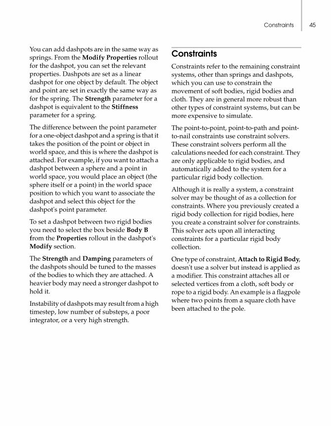
Constraints 45
You can add dashpots are in the same way as springs. From the Modify Properties rollout for the dashpot, you can set the relevant properties. Dashpots are set as a linear dashpot for one object by default. The object and point are set in exactly the same way as for the spring. The Strength parameter for a dashpot is equivalent to the Stiffness parameter for a spring.
The difference between the point parameter for a one-object dashpot and a spring is that it takes the position of the point or object in world space, and this is where the dashpot is attached. For example, if you want to attach a dashpot between a sphere and a point in world space, you would place an object (the sphere itself or a point) in the world space position to which you want to associate the dashpot and select this object for the dashpot's point parameter.
To set a dashpot between two rigid bodies you need to select the box beside Body B from the Properties rollout in the dashpot's Modify section.
The Strength and Damping parameters of the dashpots should be tuned to the masses of the bodies to which they are attached. A heavier body may need a stronger dashpot to hold it.
Instability of dashpots may result from a high timestep, low number of substeps, a poor integrator, or a very high strength.
ConstraintsConstraints refer to the remaining constraint systems, other than springs and dashpots, which you can use to constrain the movement of soft bodies, rigid bodies and cloth. They are in general more robust than other types of constraint systems, but can be more expensive to simulate.
The point-to-point, point-to-path and point-to-nail constraints use constraint solvers. These constraint solvers perform all the calculations needed for each constraint. They are only applicable to rigid bodies, and automatically added to the system for a particular rigid body collection.
Although it is really a system, a constraint solver may be thought of as a collection for constraints. Where you previously created a rigid body collection for rigid bodies, here you create a constraint solver for constraints. This solver acts upon all interacting constraints for a particular rigid body collection.
One type of constraint, Attach to Rigid Body, doesn't use a solver but instead is applied as a modifier. This constraint attaches all or selected vertices from a cloth, soft body or rope to a rigid body. An example is a flagpole where two points from a square cloth have been attached to the pole.

Chapter 8: Constraints46
Constraint SolverTo add a constraint solver to a system, select CSolver from the reactor section (Figure 8.5.1) and click in one of the view panes to place it in the scene. Using Pick and Add from the Properties rollout for the solver you can add constraints to the solver at creation or afterwards in the Modify tab.
Figure 8.5.1
You also need to associate a rigid body collection with the solver. Click the button under RBCollection within the solver's Properties section and select the collection on which the solver's constraints work. A solver can only solve constraints acting on bodies in one collection. It cannot span multiple collections.
If you add constraints that work on objects from a collection other than that associated with the solver, the Analyze World utility notifies you when you try to run the simulation.
Within the properties for the constraint solver there are three options for the type of solver you would like to use: Cheap, General and Expensive. Cheap is the least accurate but the fastest and Expensive is the most accurate but slowest. The default value is General, which handles most situations.
Figure 8.5.2
Point-to-Point ConstraintA point-to-point constraint constrains two bodies to share a common point.
1. Draw two boxes and a point somewhere near them.
2. Add them to a rigid collection.
3. In the reactor section, select Point-Point.
4. Click anywhere in the scene to add the constraint.
5. You have to add two objects and one point to the constraint using the appropriate buttons from the Properties rollout for the constraint.
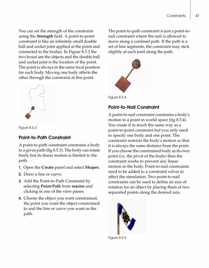
Constraints 47
You can set the strength of the constraint using the Strength field. A point-to-point constraint is like an infinitely small double ball and socket joint applied at the point and connected to the bodies. In Figure 8.5.2 the two boxes are the objects and the double ball and socket joint is the location of the point. The point is always in the same local position for each body. Moving one body affects the other through the constraint at this point.
Figure 8.5.3
Point-to-Path ConstraintA point-to-path constraint constrains a body to a given path (fig 8.5.3). The body can rotate freely but its linear motion is limited to the path.
1. Open the Create panel and select Shapes.
2. Draw a line or curve.
3. Add the Point-to-Path Constraint by selecting Point-Path from reactor and clicking in one of the view panes.
4. Choose the object you want constrained, the point you want the object constrained to and the line or curve you want as the path.
The point-to-path constraint is just a point-to-nail constraint where the nail is allowed to move along a confined path. If the path is a set of line segments, the constraint may stick slightly at each joint along the path.
Figure 8.5.4
Point-to-Nail ConstraintA point-to-nail constraint constrains a body's motion to a point in world space (fig 8.5.4). You create it in much the same way as a point-to-point constraint but you only need to specify one body and one point. The constraint restricts the body's motion so that it is always the same distance from the point. If you choose the constrained body as its own point (i.e. the pivot of the body) then the constraint works to prevent any linear motion in the body. Point-to-nail constraints need to be added to a constraint solver to affect the simulation. Two point-to-nail constraints can be used to define an axis of rotation for an object by placing them at two separated points along the desired axis.
Figure 8.5.5
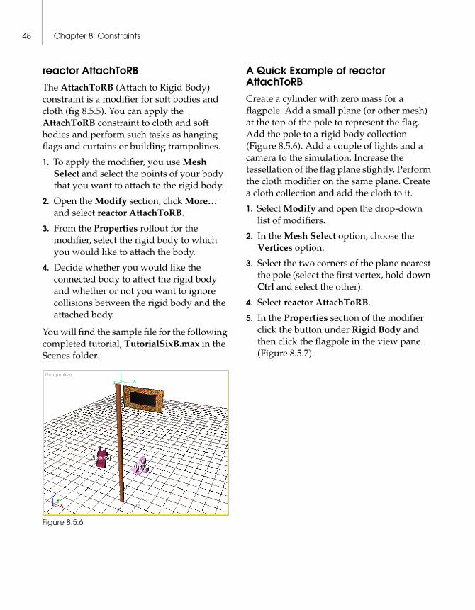
Chapter 8: Constraints48
reactor AttachToRBThe AttachToRB (Attach to Rigid Body) constraint is a modifier for soft bodies and cloth (fig 8.5.5). You can apply the AttachToRB constraint to cloth and soft bodies and perform such tasks as hanging flags and curtains or building trampolines.
1. To apply the modifier, you use Mesh Select and select the points of your body that you want to attach to the rigid body.
2. Open the Modify section, click More… and select reactor AttachToRB.
3. From the Properties rollout for the modifier, select the rigid body to which you would like to attach the body.
4. Decide whether you would like the connected body to affect the rigid body and whether or not you want to ignore collisions between the rigid body and the attached body.
You will find the sample file for the following completed tutorial, TutorialSixB.max in the Scenes folder.
Figure 8.5.6
A Quick Example of reactor AttachToRBCreate a cylinder with zero mass for a flagpole. Add a small plane (or other mesh) at the top of the pole to represent the flag. Add the pole to a rigid body collection (Figure 8.5.6). Add a couple of lights and a camera to the simulation. Increase the tessellation of the flag plane slightly. Perform the cloth modifier on the same plane. Create a cloth collection and add the cloth to it.
1. Select Modify and open the drop-down list of modifiers.
2. In the Mesh Select option, choose the Vertices option.
3. Select the two corners of the plane nearest the pole (select the first vertex, hold down Ctrl and select the other).
4. Select reactor AttachToRB.
5. In the Properties section of the modifier click the button under Rigid Body and then click the flagpole in the view pane (Figure 8.5.7).
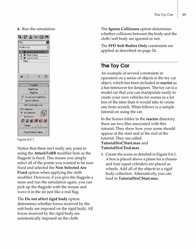
The Toy Car 49
6. Run the simulation.
Figure 8.5.7
Notice that there isn't really any point in using the AttachToRB modifier here as the flagpole is fixed. This means you simply select all of the points you wanted to be non-fixed and selected the Non Selected Are Fixed option when applying the cloth modifier. However, if you give the flagpole a mass and run the simulation again, you can pick up the flagpole with the mouse and wave it in the air just like a real flag.
The Do not affect rigid body option determines whether forces received by the soft body are imposed on the rigid body. All forces received by the rigid body are automatically imposed on the cloth.
The Ignore Collisions option determines whether collisions between the body and the cloth/soft body are ignored or not.
The FFD Soft Bodies Only constraints are applied as described on page 24.
The Toy CarAn example of several constraints in operation on a series of objects is the toy car object, which has been included in reactor as a fun timesaver for designers. The toy car is a model car that you can manipulate easily to create your own vehicles for scenes in a lot less of the time than it would take to create one from scratch. What follows is a sample tutorial on using the car.
In the Scenes folder in the reactor directory, there are two files associated with this tutorial. They show how your scene should appear at the start and at the end of the tutorial. They are called TutorialSixCStart.max and TutorialSixCEnd.max.
1. Create the scene as detailed in Figure 8.6.1. A box is placed above a plane for a chassis and four equal cylinders are placed as wheels. Add all of the objects to a rigid body collection. Alternatively, you can load in TutorialSixCStart.max.
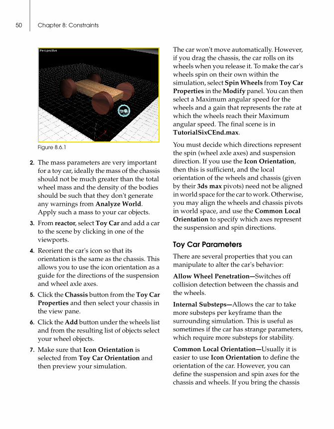
Chapter 8: Constraints50
Figure 8.6.1
2. The mass parameters are very important for a toy car, ideally the mass of the chassis should not be much greater than the total wheel mass and the density of the bodies should be such that they don't generate any warnings from Analyze World. Apply such a mass to your car objects.
3. From reactor, select Toy Car and add a car to the scene by clicking in one of the viewports.
4. Reorient the car's icon so that its orientation is the same as the chassis. This allows you to use the icon orientation as a guide for the directions of the suspension and wheel axle axes.
5. Click the Chassis button from the Toy Car Properties and then select your chassis in the view pane.
6. Click the Add button under the wheels list and from the resulting list of objects select your wheel objects.
7. Make sure that Icon Orientation is selected from Toy Car Orientation and then preview your simulation.
The car won't move automatically. However, if you drag the chassis, the car rolls on its wheels when you release it. To make the car's wheels spin on their own within the simulation, select Spin Wheels from Toy Car Properties in the Modify panel. You can then select a Maximum angular speed for the wheels and a gain that represents the rate at which the wheels reach their Maximum angular speed. The final scene is in TutorialSixCEnd.max.
You must decide which directions represent the spin (wheel axle axes) and suspension direction. If you use the Icon Orientation, then this is sufficient, and the local orientation of the wheels and chassis (given by their 3ds max pivots) need not be aligned in world space for the car to work. Otherwise, you may align the wheels and chassis pivots in world space, and use the Common Local Orientation to specify which axes represent the suspension and spin directions.
Toy Car ParametersThere are several properties that you can manipulate to alter the car's behavior:
Allow Wheel Penetration—Switches off collision detection between the chassis and the wheels.
Internal Substeps—Allows the car to take more substeps per keyframe than the surrounding simulation. This is useful as sometimes if the car has strange parameters, which require more substeps for stability.
Common Local Orientation—Usually it is easier to use Icon Orientation to define the orientation of the car. However, you can define the suspension and spin axes for the chassis and wheels. If you bring the chassis

The Toy Car 51
and wheel pivots to a common orientation then with respect to this orientation you can manually set the axes for suspension and spin with the respective options.
Angular Strength—This represents the strength of the corrective forces applied to keep the wheels upright and pointing forwards.
Linear Strength—This represents the strength of the forces applied to keep the wheels in position relative to the chassis.
Suspension—Sets the stiffness of the suspension for the car. The lower the value the more the chassis will bounce while having forces applied to it.
Disabled—Removes the car from the simulation.

Chapter 8: Constraints52
ActionsAction is a group name used to describe several complex physical systems that are available to you in reactor™ . They are grouped under this name simply to differentiate them from constraint and water systems. The action systems allow you to simulate wind, motors and fractures in scenes.
This chapter takes you through the process of learning about each of the different types of action.
About This TutorialDuring this tutorial you will see the actions that have been included in reactor. By the end of this chapter you will:
• Know the various types of action available to you in the plug-in
• Be able to implement these Actions in your scenes
The completed files for the tutorials at the end of the chapter are included in the Scenes folder. They are TutorialSevenA.max, TutorialSevenB.max and TutorialSevenC.max.
The Actionsreactor currently comes with three actions, each of which is detailed below.
Wind ActionThis adds wind to a scene. Wind is represented by the symbol of a weather vane. The direction of the rooster determines the direction of the wind. You can decide which types of object the wind affects, be they cloth, soft or rigid. You can also set the wind speed, introduce variance into the wind's strength, apply a ripple to the wind along an axis and apply a variance to this ripple. You can also activate the ability of objects to gain shelter from the wind due to the position of other objects.
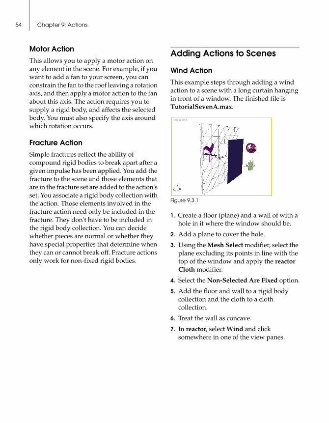
Chapter 9: Actions54
Motor ActionThis allows you to apply a motor action on any element in the scene. For example, if you want to add a fan to your screen, you can constrain the fan to the roof leaving a rotation axis, and then apply a motor action to the fan about this axis. The action requires you to supply a rigid body, and affects the selected body. You must also specify the axis around which rotation occurs.
Fracture ActionSimple fractures reflect the ability of compound rigid bodies to break apart after a given impulse has been applied. You add the fracture to the scene and those elements that are in the fracture set are added to the action's set. You associate a rigid body collection with the action. Those elements involved in the fracture action need only be included in the fracture. They don't have to be included in the rigid body collection. You can decide whether pieces are normal or whether they have special properties that determine when they can or cannot break off. Fracture actions only work for non-fixed rigid bodies.
Adding Actions to Scenes
Wind ActionThis example steps through adding a wind action to a scene with a long curtain hanging in front of a window. The finished file is TutorialSevenA.max.
Figure 9.3.1
1. Create a floor (plane) and a wall of with a hole in it where the window should be.
2. Add a plane to cover the hole.
3. Using the Mesh Select modifier, select the plane excluding its points in line with the top of the window and apply the reactor Cloth modifier.
4. Select the Non-Selected Are Fixed option.
5. Add the floor and wall to a rigid body collection and the cloth to a cloth collection.
6. Treat the wall as concave.
7. In reactor, select Wind and click somewhere in one of the view panes.

Adding Actions to Scenes 55
8. Rotate the symbol for the wind so that the wind is blowing towards your window.
9. Select the Enable Sheltering option. (Figure 9.3.2).
Figure 9.3.2
10.Make sure that only cloth is selected in the Applies To... section.
Preview the simulation. The wind should blow through the window and affect the curtain. By selecting Perturb Speed, you can modify the wind's strength. The Variance value varies smoothly over time. The Time Scale determines how quickly this occurs, with small values producing a slow change and large values producing rapid change.
With the Ripple check box selected, the direction becomes a function of space and time. This effect can occur in the Left/Right, Up/Down or Back/Forward directions with Forward being along the wind direction, and Up being the up-axis of the wind icon. For example, a curtain hanging down might require ripples active in the Left/Right direction.
The Magnitude determines the directional variance and the Frequency determines the regularity of ripple formation. Low values means distant ripples, high values means closely packed ripples.
If the Perturb Time check box is selected, the spatial perturbation is itself perturbed over time, which causes the ripples to move back and forth. If this is not checked, the cloth should come to rest, unless Perturb Speed is checked.

Chapter 9: Actions56
Motor ActionIn the example, you will create a windmill with spinning blades. The finished file is TutorialSevenB.max.
Figure 9.3.3
1. Create a truncated cone and reduce the number of segments to four to create a windmill.
2. Make some blades as a compound rigid body.
3. Constrain the blades in front of the windmill and along the axis of rotation using two point-to-nail constraints. Set the constraints strengths to 50. (Figure 9.3.3).
4. Add a CSolver system and add the constraints to it.
5. Add a Motor Action to the scene from reactor. Set the Ang Speed to 10.0 and the Gain to 3.0.
6. Click the rigid body button in the motor action's Properties rollout (Figure 9.3.4) and select the blades.
7. In the dropdown menu for the coordinate reference system, select Local.
8. Select the blades and set which axis represents the one around which you want the blades to rotate (in body space).
9. Select the Motor symbol and, in the Modify section for the motor, select the axis that you noted for the blades.
Figure 9.3.4
Preview the simulation. The blades should spin. The Ang. Speed is the speed the motor tries to maintain, and the Gain is how fast it recovers when blockage or other forces slow the blade.
Fracture ActionThe following short tutorial creates a table and breaks it during a simulation using the fracture action. The finished file is TutorialSevenC.max.
1. Create a table and give each element mass as though you were going to create a compound rigid body, but don't actually group them.
2. Create a plane onto which the table can fall. Create a rigid body collection and add only the plane to it (Figure 9.3.5). Add the Fracture Action to the scene from the reactor options.
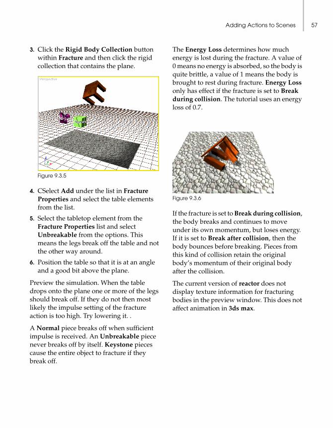
Adding Actions to Scenes 57
3. Click the Rigid Body Collection button within Fracture and then click the rigid collection that contains the plane.
Figure 9.3.5
4. CSelect Add under the list in Fracture Properties and select the table elements from the list.
5. Select the tabletop element from the Fracture Properties list and select Unbreakable from the options. This means the legs break off the table and not the other way around.
6. Position the table so that it is at an angle and a good bit above the plane.
Preview the simulation. When the table drops onto the plane one or more of the legs should break off. If they do not then most likely the impulse setting of the fracture action is too high. Try lowering it. .
A Normal piece breaks off when sufficient impulse is received. An Unbreakable piece never breaks off by itself. Keystone pieces cause the entire object to fracture if they break off.
The Energy Loss determines how much energy is lost during the fracture. A value of 0 means no energy is absorbed, so the body is quite brittle, a value of 1 means the body is brought to rest during fracture. Energy Loss only has effect if the fracture is set to Break during collision. The tutorial uses an energy loss of 0.7.
Figure 9.3.6
If the fracture is set to Break during collision, the body breaks and continues to move under its own momentum, but loses energy. If it is set to Break after collision, then the body bounces before breaking. Pieces from this kind of collision retain the original body’s momentum of their original body after the collision.
The current version of reactor does not display texture information for fracturing bodies in the preview window. This does not affect animation in 3ds max.

Chapter 9: Actions58

Animationreactor™ has the ability to feed physical simulations into keyframed animation. It is often an intricate process to achieve the ideal blend of keyframed animation and physical simulation, and reactor provides a number of mechanisms for helping you to get the most from reactor physics.
At a basic level, the physical simulation can assume control of the entire scene and feed directly into the 3ds max™ 4 animation. At a more sophisticated level, keyframed bodies can interact with the physical simulation.
About This TutorialThis tutorial deals with animating in 3ds max using reactor. There are several ways that you can animate objects, while capturing the physical simulation data. These range from simple animations that are entirely composed of physical data, to more sophisticated animations in which there is a mix of keyframed and physical bodies.
By the end of the tutorial you will be able to
• Create a physical animation
• Use 3ds max Keyframes with reactor
• Use unyielding bodies
• Interact with your scene and update 3ds max to reflect the interactions
Creating a Simple AnimationYou can create a simple animation by following these simple steps. The tutorial creates a series of balls rolling down a ramp and into a bucket1.
Figure 10.1.1
1. In some demo versions of reactor, you cannot simulate this many bodies for the specified number of frames.
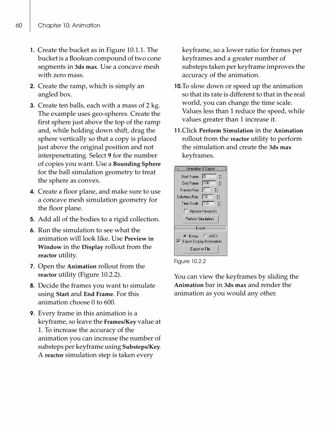
Chapter 10: Animation60
1. Create the bucket as in Figure 10.1.1. The bucket is a Boolean compound of two cone segments in 3ds max. Use a concave mesh with zero mass.
2. Create the ramp, which is simply an angled box.
3. Create ten balls, each with a mass of 2 kg. The example uses geo-spheres. Create the first sphere just above the top of the ramp and, while holding down shift, drag the sphere vertically so that a copy is placed just above the original position and not interpenetrating. Select 9 for the number of copies you want. Use a Bounding Sphere for the ball simulation geometry to treat the sphere as convex.
4. Create a floor plane, and make sure to use a concave mesh simulation geometry for the floor plane.
5. Add all of the bodies to a rigid collection.
6. Run the simulation to see what the animation will look like. Use Preview in Window in the Display rollout from the reactor utility.
7. Open the Animation rollout from the reactor utility (Figure 10.2.2).
8. Decide the frames you want to simulate using Start and End Frame. For this animation choose 0 to 600.
9. Every frame in this animation is a keyframe, so leave the Frames/Key value at 1. To increase the accuracy of the animation you can increase the number of substeps per keyframe using Substeps/Key. A reactor simulation step is taken every
keyframe, so a lower ratio for frames per keyframes and a greater number of substeps taken per keyframe improves the accuracy of the animation.
10.To slow down or speed up the animation so that its rate is different to that in the real world, you can change the time scale. Values less than 1 reduce the speed, while values greater than 1 increase it.
11.Click Perform Simulation in the Animation rollout from the reactor utility to perform the simulation and create the 3ds max keyframes.
Figure 10.2.2
You can view the keyframes by sliding the Animation bar in 3ds max and render the animation as you would any other.
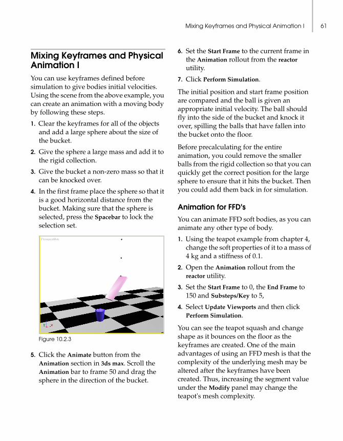
Mixing Keyframes and Physical Animation I 61
Mixing Keyframes and Physical Animation IYou can use keyframes defined before simulation to give bodies initial velocities. Using the scene from the above example, you can create an animation with a moving body by following these steps.
1. Clear the keyframes for all of the objects and add a large sphere about the size of the bucket.
2. Give the sphere a large mass and add it to the rigid collection.
3. Give the bucket a non-zero mass so that it can be knocked over.
4. In the first frame place the sphere so that it is a good horizontal distance from the bucket. Making sure that the sphere is selected, press the Spacebar to lock the selection set.
Figure 10.2.3
5. Click the Animate button from the Animation section in 3ds max. Scroll the Animation bar to frame 50 and drag the sphere in the direction of the bucket.
6. Set the Start Frame to the current frame in the Animation rollout from the reactor utility.
7. Click Perform Simulation.
The initial position and start frame position are compared and the ball is given an appropriate initial velocity. The ball should fly into the side of the bucket and knock it over, spilling the balls that have fallen into the bucket onto the floor.
Before precalculating for the entire animation, you could remove the smaller balls from the rigid collection so that you can quickly get the correct position for the large sphere to ensure that it hits the bucket. Then you could add them back in for simulation.
Animation for FFD'sYou can animate FFD soft bodies, as you can animate any other type of body.
1. Using the teapot example from chapter 4, change the soft properties of it to a mass of 4 kg and a stiffness of 0.1.
2. Open the Animation rollout from the reactor utility.
3. Set the Start Frame to 0, the End Frame to 150 and Substeps/Key to 5,
4. Select Update Viewports and then click Perform Simulation.
You can see the teapot squash and change shape as it bounces on the floor as the keyframes are created. One of the main advantages of using an FFD mesh is that the complexity of the underlying mesh may be altered after the keyframes have been created. Thus, increasing the segment value under the Modify panel may change the teapot's mesh complexity.
Chapter 10: Animation62
Mixing Keyframes and Physical Animation IIYou can keyframe the motion of objects using standard 3ds max tools, and physically simulate the same frames without any fear of your keyframed motion being affected.
Selecting the Unyielding property in the Properties rollout from the reactor utility specifies that an object is unaffected by collisions with other objects. Other objects will naturally bounce off the unyielding object. This method is preferable for accurate simulations instead of the alternative of not including the objects in the rigid body collection and keyframing them (since this would result in them not interacting at all with any physical objects and appearing to pass right through them). Unyielding objects are otherwise normal objects and you may attach springs and dashpots to them.
In the Advanced rollout from the reactor utility there is an option called Unyielding: Updates/Frame. Before starting a simulation, reactor locates the position and orientation of the unyielding bodies at different times. During the simulation, the engine will interpolate between these positions & orientations. The number of positions taken from 3ds max is set with the parameter Updates/Frame. You don't normally need to change this value. Decreasing it speeds up the animation, and increasing it has the opposite effect. Sometimes increasing this value is necessary to correct the motion of a body.
If you want to include an object in a scene and are only interested in the body's own motion you can ignore collisions for the body by selecting Disable All Collisions from the Properties rollout.
Deforming MeshesWhen animating characters, a common approach is to use a modifier that applies a skin-and-bones to the character. A Skin modifier deforms a mesh according to the movement of its component parts (the bones). The skin mesh wraps around the bones. So, in animating a character, you actually animate the bones, and the skin merely follows the shape that the bones dictate. Bones are usually simplified since they are not actually displayed. They merely dictate motion.
From a reactor point of view, skins are part of a larger subset of object types called Deforming Meshes. A deforming mesh is any body whose position, orientation and shape are all completely controlled by 3ds max. You define motion and deformation in 3ds max, but want to use that completely scripted motion to affect other bodies.
You can add deforming meshes as parts of a deforming mesh collection. You can create a deforming mesh collection using the DMCollection button in the reactor menu, much like any other collection. They are physically simulated as part of their collections, and can thus affect other physical bodies, but still have their shapes and positions completely controlled by 3ds max, and are not themselves affected by the physics.

Keyframe Reduction 63
Deforming Mesh PropertiesThe following is a list of the properties specific to deforming meshes.
Updates/Frame—This parameter allows you to specify how often reactor asks 3ds max for the position of the object. Higher values are more accurate, but they take a longer time to simulate. Low values can result in inaccurate simulation.
Freeze—The Freeze check box disables updates of any objects in the collection. In so doing, you set the objects to behave as fixed rigid bodies. This is useful for situations in which you want other objects to settle on top of the deformed mesh before an animation begins.
Keyframe ReductionWhen composing animations, it is common for many of the keyframes to be relatively redundant. However, these redundant keyframes are still factored into the creation process, which can result in large uses of memory and disk space. It is for this reason that reactor includes a feature called keyframe reduction.
Keyframe reduction enables you to assign specific keyframes to objects. For example, you can tell a rigid body its positions in a couple of frames (perhaps frame 0, frame 25 and frame 90), and 3ds max interpolates the frames in between the ones you have specified. This affords you a high level of control, while also considerably reducing system resource usage.
You can use any of the following options to reduce keyframe animations in a scene.
• The Reduce Keyframes button in the Properties rollout reduces keyframes for selected rigid bodies.
• The Delete Keyframes button in the Properties menu deletes all the keyframes for selected rigid bodies.
• The Start/End Frame options in the Simulation rollout ensure that any reduction or deletion you want to perform only occurs between the intervals you specify.
• The Reduce Now button in the Advanced rollout reduces keyframes for all the rigid bodies in a simulation.
• The Reduce After Simulation option in the Advanced rollout ensures that when you run simulations, keyframe reduction occurs automatically.
• The Delete Now button in the Advanced rollout deletes all the keyframes for selected rigid bodies in a simulation.

Chapter 10: Animation64
Interactive ModificationQuite often, the scene you will want to work with is not the one you designed in 3ds max. You may have designed a scene with the objects above the ground, but want them in their natural rest position. You may also want to reflect other physical changes such as folds in draping curtains.
You can use the Update Max function to translate physical changes in the simulation back to 3ds max. When running a simulation in a window, wait until the objects in the scene have attained the states that you want to translate back to 3ds max, open the Max menu and select Update Max (see Figure 10.7.1).
Figure 10.7.1
When you close the preview window and click one of the view panes, the scene is updated. No update of 3ds max can be done until the preview window is closed.
In addition, the Use Max Parameters option resets the simulation window to use the timestep and substeps specified in the Animation rollout, and the total Animation Time specified by 3ds max.

IntroductionThis section discusses the use of MAXScript with the reactor™ plug-in. It assumes a basic working knowledge of the scripting language. You can access full information on MAXScript in MAXScript Reference… option of the Help menu.
You can enter sections of script into the 3ds max™ built-in listener for testing and experimentation. To start the MAXScript Listener, press F11. Alternatively, you or use the MAXScript Listener… option from the MAXScript menu. (See Figure 11.1.)
Figure 11.1
reactor ObjectsYou can create many of the objects available with the reactor plug-in through MAXScript. You can also access many of the properties from the rollouts through scripting. You can display accessible reactor objects using the following MAXScript commands:apropos "HK*"apropos "Havok*"
At time of writing these commands display the following lists of objects:apropos "Havok*"
HavokSetGravity (const Primitive): Havok-SetGravity()
HavokGetGravity (const Primitive): HavokGetGravity()
HavokDeleteAllKeys (const Primitive): HavokDeleteAllKeys()
HavokReduceAllKeys (const Primitive): HavokReduceAllKeys()
HavokReduceSelectedKeys (const Primi-tive): apropos "HK*"
HKWaterWSM (const MaxClass): Havok_Water
HKRBCollection (const MaxClass): RBCol-lection
HKConstraintSolver (const MaxClass): CSolver
Chapter 11: MAXScript and reactor66
HKPointToNail (const MaxClass): Point_Nail
HKPointToPath (const MaxClass): Point_Path
HKPointToPoint (const MaxClass): Point_Point
HKDMCollection (const MaxClass): DMCol-lection
HKMotor (const MaxClass): Motorhelper
HKCLCollection (const MaxClass): CLCol-lection
HKWind (const MaxClass): Windhelper
HKToyCar (const MaxClass): Toy_Car
HKSBCollection (const MaxClass): SBCol-lection
HKRPCollection (const MaxClass): RPCol-lection
HKPlane (const MaxClass): Planehelper
HKSpring (const MaxClass): Springhelper
HKFracture (const MaxClass): Fracture
HKDashpot (const MaxClass): Dashpot
HKClothModifier (const MaxClass): Havok_Cloth
HKWaterWSMObject (const MaxClass): Water
HKSoftBodyModifier (const MaxClass): Havok_SoftBody
HKRopeModifier (const MaxClass): Havok_Rope
HKAttachToRBModifier (const MaxClass): Havok_AttachToRB
HKDynamics (const MaxClass): Havok_Dynamics
OK
HavokReduceSelectedKeys()
HavokDeleteSelectedKeys (const Primi-tive): HavokDeleteSelectedKeys()
HavokTestSelectedConvexity (const Primi-tive): HavokTestSelectedConvexity()
HavokExportWorld (const Primitive): HavokExportWorld()
HavokAnalyzeWorld (const Primitive): HavokAnalyzeWorld()
HavokPerformSimulation (const Primi-tive): HavokPerformSimulation()
HavokShowInWindow (const Primitive): HavokShowInWindow()
HavokSetDirectX (const Primitive): Havok-SetDirectX()
HavokGetDirectX (const Primitive): HavokGetDirectX()
HavokSetFullScreen (const Primitive): HavokSetFullScreen()
HavokGetFullScreen (const Primitive): HavokGetFullScreen()
HavokSetMSDamping (const Primitive): HavokSetMSDamping()
HavokGetMSDamping (const Primitive): HavokGetMSDamping()
HavokSetMSRestLength (const Primitive): HavokSetMSRestLength()
HavokGetMSRestLength (const Primitive): HavokGetMSRestLength()
HavokSetMSStrength (const Primitive): HavokSetMSStrength()
HavokGetMSStrength (const Primitive): HavokGetMSStrength()
HavokSetTextureQuality (const Primi-tive): HavokSetTextureQuality()
HavokGetTextureQuality (const Primi-tive): HavokGetTextureQuality()
HavokSetCastShadowsPlane (const Primi-tive): HavokSetCastShadowsPlane()
HavokGetCastShadowsPlane (const Primi-tive): HavokGetCastShadowsPlane()
HavokSetCastShadowsCheck (const Primi-tive): HavokSetCastShadowsCheck()
HavokGetCastShadowsCheck (const Primi-tive): HavokGetCastShadowsCheck()
HavokRemoveLight (const Primitive): HavokRemoveLight()
HavokAddLight (const Primitive): HavokAd-dLight()
HavokSetCamera (const Primitive): Havok-SetCamera()
HavokGetCamera (const Primitive): HavokGetCamera()

reactor Objects 67
HavokCheckRigidRigidCollisions (const Primitive): HavokCheckRigidRigidColli-sions()
HavokEnableAllCollisions (const Primi-tive): HavokEnableAllCollisions()
HavokEnableAllRigidCollisions (const Primitive): HavokEnableAllRigidColli-sions()
HavokEnableRigidRigidCollisions (const Primitive): HavokEnableRigidRigidColli-sions()
HavokDisableAllRigidCollisions (const Primitive): HavokDisableAllRigidColli-sions()
HavokDisableRigidRigidCollisions (const Primitive): HavokDisableRigidRigidColli-sions()
HavokSetExportDisplay (const Primitive): HavokSetExportDisplay()
HavokGetExportDisplay (const Primitive): HavokGetExportDisplay()
HavokSetExportFormat (const Primitive): HavokSetExportFormat()
HavokGetExportFormat (const Primitive): HavokGetExportFormat()
HavokSetUpdateViewports (const Primi-tive): HavokSetUpdateViewports()
HavokGetUpdateViewports (const Primi-tive): HavokGetUpdateViewports()
HavokSetTimeScale (const Primitive): HavokSetTimeScale()
HavokGetTimeScale (const Primitive): HavokGetTimeScale()
HavokSetSubsteps (const Primitive): HavokSetSubsteps()
HavokGetSubsteps (const Primitive): HavokGetSubsteps()
HavokSetFramesKey (const Primitive): HavokSetFramesKey()
HavokGetFramesKey (const Primitive): HavokGetFramesKey()
HavokSetEndFrame (const Primitive): HavokSetEndFrame()
HavokGetEndFrame (const Primitive): HavokGetEndFrame()
HavokSetStartFrame (const Primitive): HavokSetStartFrame()
HavokGetStartFrame (const Primitive): HavokGetStartFrame()
HavokSetReduceAfterSimulation (const Primitive): HavokSetReduceAfterSimula-tion()
HavokGetReduceAfterSimulation (const Primitive): HavokGetReduceAfterSimula-tion()
HavokSetReductionThreshold (const Primi-tive): HavokSetReductionThreshold()
HavokGetReductionThreshold (const Primi-tive): HavokGetReductionThreshold()
HavokSetAnalyzeBeforeSimulation (const Primitive): HavokSetAnalyzeBeforeSimula-tion()
HavokGetAnalyzeBeforeSimulation (const Primitive): HavokGetAnalyzeBeforeSimula-tion()
HavokSetSaveBeforeSimulation (const Prim-itive): HavokSetSaveBeforeSimulation()
HavokGetSaveBeforeSimulation (const Prim-itive): HavokGetSaveBeforeSimulation()
HavokSetWorldScale (const Primitive): HavokSetWorldScale()
HavokGetWorldScale (const Primitive): HavokGetWorldScale()
HavokSetCollisionTolerance (const Primi-tive): HavokSetCollisionTolerance()
HavokGetCollisionTolerance (const Primi-tive): HavokGetCollisionTolerance()
HavokSetResolver (const Primitive): HavokSetResolver()
HavokGetResolver (const Primitive): HavokGetResolver()
HavokSetUnyieldUpdates (const Primi-tive): HavokSetUnyieldUpdates()
HavokGetUnyieldUpdates (const Primi-tive): HavokGetUnyieldUpdates()
HavokSetAngularDrag (const Primitive): HavokSetAngularDrag()

Chapter 11: MAXScript and reactor68
HavokGetAngularDrag (const Primitive): HavokGetAngularDrag()
HavokSetLinearDrag (const Primitive): HavokSetLinearDrag()
HavokGetLinearDrag (const Primitive): HavokGetLinearDrag()
HavokSetAddDragAction (const Primitive): HavokSetAddDragAction()
HavokGetAddDragAction (const Primitive): HavokGetAddDragAction()
OK
Typing any of the commands from the HK* list followed by a set of brackets creates a new object. For example, to create a new rigid body collection, type HKRBCollection() into the listener. This new object is always placed at the scene origin [0, 0, 0] and can be moved with the standard MAXScript commands, such asrbc = HKRBCollection()rbc.position = [10, 10, 10]
The commands from the Havok* list return or require parameters. They relate to the elements from the reactor utility, and allow you to set and check parameters. This is true for all of the above except those relating to collisions, such as HavokEnableRigidRigidCollisions - which takes the name of a rigid body collection and the two rigid bodies between which you want to enable collisions.
You can view properties specific to any of the reactor objects with the MAXScript command showProperties, followed by any variable. Using the previously created rigid body collection, typing showProperties rbc displays the following: .rigidBodiesTab (Rigid_Bodies_Tab) : node array .showText (Show_Text) : boolean .iconSize (Icon_Size) : float .displayType (Display_Type) : integer .odeSolver (ODE_Solver) : integer .refreshRate (Refresh_Rate) : float .addDeactivator (Add_Deactivator) : integer .energy : float .time : float .samples : integer
These properties generally relate directly to items on that object's Modifier rollout. For example, instead of using the Pick, Add or Delete buttons on the rigid body list in the user interface, a script may alter the rigidBodiesTab node array property as with any other MAXScript array. rbca = rbc.rigidBodiesTabrbca[1+rbca.count] = $
This short section of script assigns a variable, rbca, to the collections rigid body array and adds the currently selected object to the end of it.

Setting Physical Properties 69
Setting Physical Propertiesreactor objects have properties pertaining specifically to the reactor physics engine. These properties are assigned to any 3ds max object as user-defined properties. You can use the following MAXScript function to set the initial physical properties of any object. Thereafter, you can use the MAXScript commands setUserProp and getUserProp to access and change individual properties. function setHKProperties o \mass:1.000000\elasticity:0.300000\friction:0.300000\optimizationLevel:0.500000\unyielding:0\simulationGeometry:2\proxyGeometry:"<None>"\useDisplayProxy:0\disableCollisions:0\inactive:0\displayProxy:"<None>" = (if not undefined == o then
(setUserProp o "Mass" masssetUserProp o "Ellasticity" elasticitysetUserProp o "Friction" frictionsetUserProp o "Optimization_Level" opti-mizationLevelsetUserProp o "Unyielding" unyieldingsetUserProp o "Simulation_Geometry" simu-lationGeometrysetUserProp o "Proxy_Geometry" proxyGeom-etrysetUserProp o "Use_Display_Proxy" useDis-playProxysetUserProp o "Disable_Collisions" dis-ableCollisionssetUserProp o "Inactive" inactivesetUserProp o "Display_Proxy" display-Proxy)--if)
Running the SimulationYou can start the reactor simulation using MAXScript by calling the function HavokPerformSimulation(). See the macro script relating to the reactor toolbar for further available functions. This macro script file is called reactor.mcr and can be found in the ui/macroscripts subfolder of 3ds max program folder.
Example ScriptsThe following scripts have been included in this manual as useful examples of how to use MAXScript. The first script displays the basic physical properties of mass, elasticity and friction in a floating toolbar. This shows how you can set properties without having to go to the main reactor utility.rollout HKProperties "Properties"(local bUpdate = true
group "Physical Properties"(spinner mass "Mass" range:[0,1000000,0] scale:0.01 fieldwidth:75spinner elasticity "Elasticity" range:[0,1,0.3] scale:0.01 fieldwidth:75spinner friction "Friction" range:[0,1,0.3] scale:0.01 fieldwidth:75)
function enableAll = (mass.enabled = trueelasticity.enabled = truefriction.enabled = true)
function disableAll = (mass.enabled = falseelasticity.enabled = falsefriction.enabled = false)
Chapter 11: MAXScript and reactor70
function updateProperties =(if bUpdate then (for o in selection do(setUserPropo "Mass" mass.valuesetUserPropo "Ellasticity" elastic-ity.valuesetUserPropo "Friction" friction.value)--for)--if)
function updateRollout = (if 0 == selection.count then (disableAll()return false)--if
mass.value = 0elasticity.value = 0friction.value = 0for o in selection do(if not isKindOf o GeometryClass then(disableAll()return false)--ifif (undefined == (getUserProp o "Mass")) or (undefined == (getUserProp o "Ellastic-ity")) or(undefined == (getUserProp o "Friction")) then(setHKProperties o)--if
bUpdate = falsemass.value += getUserProp o "Mass"elasticity.value += getUserProp o "Ellas-ticity"friction.value += getUserProp o "Fric-tion"bUpdate = true)--formass.value /= selection.count
elasticity.value /= selection.countfriction.value /= selection.countenableAll())
on mass changed value do updateProper-ties()on elasticity changed value do updatePro-perties()on friction changed value do updateProp-erties()
on HKProperties open do updateRollout())
if undefined != HKDynamicsFloater then closeRolloutFloater HKDynamicsFloaterHKDynamicsFloater = newRolloutFloater "reactor" 190 300addRollout HKProperties HKDynamicsFloater
callbacks.removeScripts #selection-SetChanged id:#Havokcallbacks.addScript #selectionSetChanged "HKProperties.updateRollout()" id:#Havok
Setting Physical Properties 71
The following script converts a 3ds max IK chain into a reactor constraint tree.--tau - strength of constraints--twoway- whether to create bi-direc-tional constraints--N.B. leaf objects of chain are --automatically linked two-way-- ga - grouping array
global tau = 15.0global twoway = false
global ga = #()
function createPointPoint o1 o2 p = (pp = Point_Point()pp.name = o1.name + o2.name + "P2P"pp.rigidBodyA = o1 pp.rigidBodyB = o2 pp.point = ppp.tau = tau
pp.position = (o1.position + o2.position) / 2
return pp)
-- __MaxIK2reactorKConstraint-- parameters: --rbc- rigid body collection--cs - constraint solver --o - head of IK chain--function __MaxIK2reactorConstraint rbc cs o = (rbca = rbc.rigidBodiesTabrbca[1+rbca.count] = o
if undefined == getUserProp o "Mass" then setHKProperties o
-- end of chainif 0 == o.children.count then return false
csa = cs.constraintsTabfor c in o.children do(
p = Point()p.position = (o.position + c.position) / 2append ga p
pp = createPointPoint o c pcsa[1+csa.count] = pp
__MaxIK2HavokConstraint rbc cs c
if twoway then (p.position = ((o.position*1) + (c.posi-tion*2)) / 3
p = Point()p.position = ((o.position*2) + (c.posi-tion*1)) / 3append ga ppp.position -= [1, 1, 1]pp = createPointPoint c o p csa[1+csa.count] = pppp.position += [1, 1, 1]))
return true)mapped function MaxIK2HavokConstraint o =(if (undefined == o) or (0 == o.chil-dren.count) then(--messageBox "Select the head of an linked object chain"return false)
ga = #()
rbc = RBCollection()rbc.name = o.name + "RBCollection"move rbc (o.position - [5, 5, 5])
cs = CSolver()cs.name = o.name + "CSolver"cs.rbCollectionNode = rbcmove cs (o.position + [5, 5, 5])__MaxIK2HavokConstraint rbc cs o
join ga #( cs, rbc )

Chapter 11: MAXScript and reactor72
join ga cs.constraintsTab
g = group gag.name = o.name + "ConstraintGroup"setGroupOpen g true)-- * after using this utility make sure that all the bodies in the -- collection have the collisions with each other disabled.-- * see advanced tab in RBCollection-- * also add new RBCollection and CSolver to simulationutility HKConstrainIK "Constrain IK Chain with Points"(button bConstrain "Constrain"checkbox cbTwoway "two-way"spinner sTau "strength:" range:[0,1000,15]
on bConstrain pressed do(if 0 == selection.count then(messageBox "Select someting!")else(tau = sTau.valuetwoway = cbTwoway.checkedundo on (MaxIK2HavokConstraint selection ))))
Running ScriptsOnce you have written MAXScripts, they are generally saved in text files with a .ms extension in the Scripts subdirectory. You can then access these scripts through the MAXScript utility rollout. To do this, you open the Utility panel and click the MAXScript utility button.
Using the Run button, try selecting the HKPropertiesFloater.ms script file. You can now alter the basic rigid body properties in this dialog box rather than the reactor utility rollout.
Running the second sample script in the file HKConstrainIKwithPoints.ms adds an item into the MAXScript utilities list.
In the Scenes folder in the reactor directory, there are two files associated with this tutorial. They show how your scene should appear at the start and at the end of the tutorial. They are called TutorialScriptStart.max and TutorialScriptEnd.max.
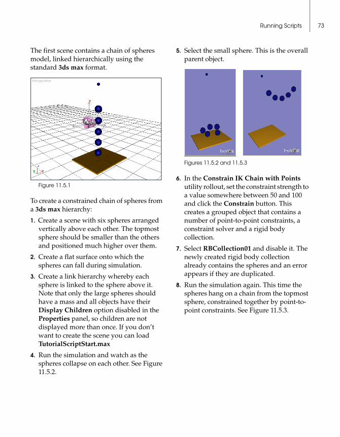
Running Scripts 73
The first scene contains a chain of spheres model, linked hierarchically using the standard 3ds max format.
Figure 11.5.1
To create a constrained chain of spheres from a 3ds max hierarchy:
1. Create a scene with six spheres arranged vertically above each other. The topmost sphere should be smaller than the others and positioned much higher over them.
2. Create a flat surface onto which the spheres can fall during simulation.
3. Create a link hierarchy whereby each sphere is linked to the sphere above it. Note that only the large spheres should have a mass and all objects have their Display Children option disabled in the Properties panel, so children are not displayed more than once. If you don’t want to create the scene you can load TutorialScriptStart.max
4. Run the simulation and watch as the spheres collapse on each other. See Figure 11.5.2.
5. Select the small sphere. This is the overall parent object.
Figures 11.5.2 and 11.5.3
6. In the Constrain IK Chain with Points utility rollout, set the constraint strength to a value somewhere between 50 and 100 and click the Constrain button. This creates a grouped object that contains a number of point-to-point constraints, a constraint solver and a rigid body collection.
7. Select RBCollection01 and disable it. The newly created rigid body collection already contains the spheres and an error appears if they are duplicated.
8. Run the simulation again. This time the spheres hang on a chain from the topmost sphere, constrained together by point-to-point constraints. See Figure 11.5.3.

Chapter 11: MAXScript and reactor74

World ScaleYou can use 3ds max™ to model a wide range of objects. You can also use different units, as meters, inches, or 3ds max generic units. From the visual point of view the scale and units you use make no difference. However, the physical representation of your objects depends on the units used. The units determine the objects' size in the physical world.
The plug-in function, Analyze World, will give you warnings if it detects that you are using extremely strange values (gravity very high, objects very big but with small mass, etc.). However a good understanding of how to use different units and scales in the plug-in will decrease your effort, and help you design accurate simulations more quickly. This is the aim of this section.
World ScaleIn order to create proper simulations, the reactor™ plug-in must know the correspondence between your units and real-world measurements. You can set this correspondence using the World Scale option in the Advanced rollout (Figure 12.1.1).
You can design your scenes to any scale, using any units you want. By setting the ratio between 1 unit in the 3ds max world and 1 meter in the physical world, you can easily control the size of your objects in the physical simulation.
For example, if you designed a scene in meters with objects twice the size that you want for simulation, then you could then set World Scale to 1m = 2.0m.

Chapter 12: World Scale76
Figure 12.1.1
If you design a scene in inches at real size, then set 1m=39.37.
Be aware that any linear values in the scene such as gravity, or rest length of springs, are interpreted using your units. That means that gravity in your "double size world" should be 19.62 m/s2 (i.e. twice the normal gravity of 9.81 m/s2).
Collision ToleranceOne of the processes during dynamics simulation is called collision detection. This means the detection of when two objects are colliding in the scene. A global value, the collision tolerance, specifies the minimum safe distance between two objects. If they are closer than this safe distance allows, they are considered to be colliding. This allows
another process, called collision resolution to react by applying forces to the objects involved and bouncing them away from each other.
In general, the higher the value of the collision tolerance, the more stable the simulation will be. However, setting too high a value for collision tolerance could lead to a noticeable gap between objects.
You need to strike a balance between stability and visual effect. There is another variable in the equation that also affects the overall stability of the system. The number of substeps taken during every simulation step can counteract the effects of a small tolerance.
So it is recommended to set the collision tolerance to the highest value at which it does not visually affect the scene. If this appears unacceptable during simulation due to unstable object collisions, increase the number of substeps in the simulation.
For instance, if your scene consists of many objects in a room, a tolerance around 0.1m should be fine. However, if the objects in your scene are dice on a table a smaller tolerance, say 0.01m or less, is preferable. If your objects are cars or buildings, a higher tolerance applies. Collision tolerance is measured in user units. That means that the world scale affects its actual value.
Advanced Simulation OptionsThis chapter covers all of the Advanced rollout options.
Add Drag ActionAdding a drag action to the system ensures that rigid bodies are subject to constant drag. This damps their linear and angular velocities, so they come to rest sooner.
For example, it is highly desirable to introduce drag whenever constraints join rigid bodies, since otherwise the constraint system may never come to rest if perturbed. The parameters Lin and Ang determine the linear and angular damping applied, respectively.
A drag action does not apply to entities other than rigid bodies.
Unyielding BodiesAlters interpolation properties of keyframed bodies. See page 62.
Collision ToleranceThe collision tolerance determines how close objects may approach before they are considered to have collided. See page 76 for details.
Resolverreactor™ allows you to choose the method of collision resolution (see page 76) using one of four resolvers: Naïve, No Friction, Simple Friction or Complex Friction.
Naïve—Reverses velocities of approaching objects. This is very fast, but very inaccurate.
No Friction—Performs proper Newtonian resolution using the coefficients of restitution, but ignores all friction values for objects in the scene. Objects tend to slide across each other.
Simple or Complex Friction—Performs proper Newtonian resolution using the coefficients of restitution and simple and complex models of friction respectively. Simple is less computationally expensive, but less accurate.

Chapter 13: Advanced Simulation Properties78
You will probably not need to alter the resolver from complex friction unless you wish to trade accuracy for speed.
World ScaleThis controls how units in 3ds max are interpreted as real-world measurements during simulation. It defines the scale of your physical objects.
Save Before SimulationCheck this box if you want 3ds max to try and save your scene every time you perform a simulation.
World AnalysisThe Analyze World button allows you to test the scene for any suspicious or odd parameters or configurations.
You can check the Analyze before simulation check box if you want to perform the Analyze World test every time you perform a simulation. The default is that this test should be performed.
Key ManagementThis section allows you to reduce duplicate or similar keyframes while retaining a visually identical animation.
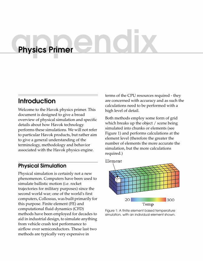
IntroductionWelcome to the Havok physics primer. This document is designed to give a broad overview of physical simulation and specific details about how Havok technology performs these simulations. We will not refer to particular Havok products, but rather aim to give a general understanding of the terminology, methodology and behavior associated with the Havok physics engine.
Physical SimulationPhysical simulation is certainly not a new phenomenon. Computers have been used to simulate ballistic motion (i.e. rocket trajectories for military purposes) since the second world war; one of the world's first computers, Collossus, was built primarily for this purpose. Finite element (FE) and computational fluid dynamics (CFD) methods have been employed for decades to aid in industrial design, to simulate anything from vehicle crash test performance to airflow over semiconductors. These last two methods are typically very expensive in
terms of the CPU resources required - they are concerned with accuracy and as such the calculations need to be performed with a high level of detail.
Both methods employ some form of grid which breaks up the object / scene being simulated into chunks or elements (see Figure 1) and performs calculations at the element level (therefore the greater the number of elements the more accurate the simulation, but the more calculations required.)
Figure 1: A finite element based temperature simulation, with an individual element shown.
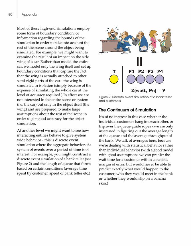
Appendix80
Most of these high-end simulations employ some form of boundary condition, or information regarding the bounds of the simulation in order to take into account the rest of the scene around the object being simulated. For example, we might want to examine the result of an impact on the side wing of a car. Rather than model the entire car, we model only the wing itself and set up boundary conditions that capture the fact that the wing is actually attached to other semi-rigid parts of the car - the wing is simulated in isolation (simply because of the expense of simulating the whole car at the level of accuracy required.) In effect we are not interested in the entire scene or system (i.e. the car) but only in the object itself (the wing) and are prepared to make large assumptions about the rest of the scene in order to get good accuracy for the object simulation.
At another level we might want to see how interacting entities behave to give system wide behavior - this is discrete event simulation where the aggregate behavior of a system of events over a period of time is of interest. For example, you might construct a discrete event simulation of a bank teller (see Figure 2) and the length of queue that forms based on certain conditions (average time spent by customer, speed of bank teller etc.)
Figure 2: Discrete event simulation of a bank teller and customers
The Continuum of SimulationIt's of no interest in this case whether the individual customers bang into each other, or trip over the queue guide ropes - we are only interested in figuring out the average length of the queue and the average throughput of the bank. We talk of averages here, because we're dealing with statistical behavior rather than individual behavior (with a good model with good assumptions we can predict the wait time for a customer within a statistic margin of error, but would never be able to predict exactly what would happen to the customer; who they would meet in the bank or whether they would slip on a banana skin.)
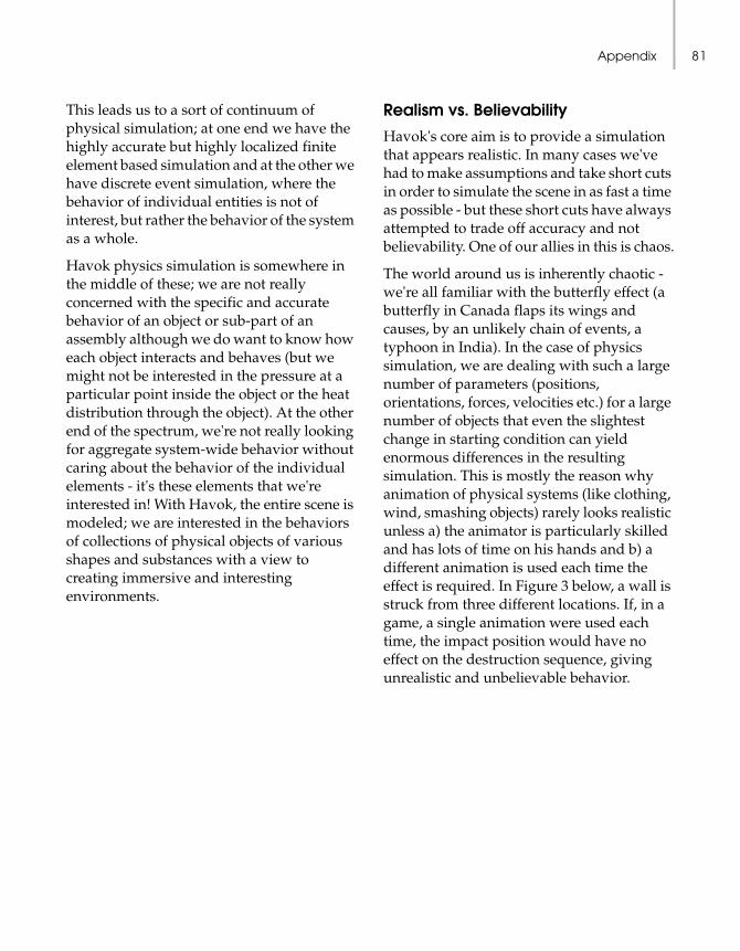
Appendix 81
This leads us to a sort of continuum of physical simulation; at one end we have the highly accurate but highly localized finite element based simulation and at the other we have discrete event simulation, where the behavior of individual entities is not of interest, but rather the behavior of the system as a whole.
Havok physics simulation is somewhere in the middle of these; we are not really concerned with the specific and accurate behavior of an object or sub-part of an assembly although we do want to know how each object interacts and behaves (but we might not be interested in the pressure at a particular point inside the object or the heat distribution through the object). At the other end of the spectrum, we're not really looking for aggregate system-wide behavior without caring about the behavior of the individual elements - it's these elements that we're interested in! With Havok, the entire scene is modeled; we are interested in the behaviors of collections of physical objects of various shapes and substances with a view to creating immersive and interesting environments.
Realism vs. BelievabilityHavok's core aim is to provide a simulation that appears realistic. In many cases we've had to make assumptions and take short cuts in order to simulate the scene in as fast a time as possible - but these short cuts have always attempted to trade off accuracy and not believability. One of our allies in this is chaos.
The world around us is inherently chaotic - we're all familiar with the butterfly effect (a butterfly in Canada flaps its wings and causes, by an unlikely chain of events, a typhoon in India). In the case of physics simulation, we are dealing with such a large number of parameters (positions, orientations, forces, velocities etc.) for a large number of objects that even the slightest change in starting condition can yield enormous differences in the resulting simulation. This is mostly the reason why animation of physical systems (like clothing, wind, smashing objects) rarely looks realistic unless a) the animator is particularly skilled and has lots of time on his hands and b) a different animation is used each time the effect is required. In Figure 3 below, a wall is struck from three different locations. If, in a game, a single animation were used each time, the impact position would have no effect on the destruction sequence, giving unrealistic and unbelievable behavior.

Appendix82
An enormous amount of time is dedicated to mimicking chaos in animation playback, particularly for real-time systems where the animations may be played many times (we are very unforgiving of looped or repeated animations.) In a game, if a character falls in exactly the same way each time it is killed, our belief that we are playing in a real environment (albeit as fantastical as the game scenario dictates) is negatively affected.
With a physics engine, you get this expected chaotic behavior by default and this is the primary reason for using this technology.
ScalePhysics, as a body of knowledge, is enormous. What we are concerned with here would more accurately be described as a mechanical simulation of the interactions of objects at real world scales. We are dealing with Newtonian mechanics, that is, the well understood laws of motion, popularized by Sir Isaac Newton, that describe the behavior of objects under the influences of other objects and external forces. Since then we've discovered that these laws break down at really small (i.e. subatomic) and really large (i.e. planetary) scales.
Figure 3: Chaotic behavior of a smashing wall impacted at different locations
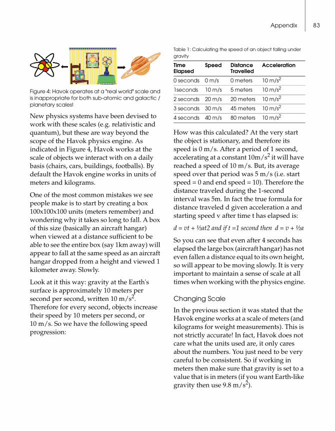
Appendix 83
Figure 4: Havok operates at a "real world" scale and is inappropriate for both sub-atomic and galactic / planetary scales!
New physics systems have been devised to work with these scales (e.g. relativistic and quantum), but these are way beyond the scope of the Havok physics engine. As indicated in Figure 4, Havok works at the scale of objects we interact with on a daily basis (chairs, cars, buildings, footballs). By default the Havok engine works in units of meters and kilograms.
One of the most common mistakes we see people make is to start by creating a box 100x100x100 units (meters remember) and wondering why it takes so long to fall. A box of this size (basically an aircraft hangar) when viewed at a distance sufficient to be able to see the entire box (say 1km away) will appear to fall at the same speed as an aircraft hangar dropped from a height and viewed 1 kilometer away. Slowly.
Look at it this way: gravity at the Earth's surface is approximately 10 meters per second per second, written 10 m/s2. Therefore for every second, objects increase their speed by 10 meters per second, or 10 m/s. So we have the following speed progression:
Table 1: Calculating the speed of an object falling under gravity
How was this calculated? At the very start the object is stationary, and therefore its speed is 0 m/s. After a period of 1 second, accelerating at a constant 10m/s2 it will have reached a speed of 10 m/s. But, its average speed over that period was 5 m/s (i.e. start speed = 0 and end speed = 10). Therefore the distance traveled during the 1-second interval was 5m. In fact the true formula for distance traveled d given acceleration a and starting speed v after time t has elapsed is:
d = vt + ½at2 and if t =1 second then d = v + ½a
So you can see that even after 4 seconds has elapsed the large box (aircraft hangar) has not even fallen a distance equal to its own height, so will appear to be moving slowly. It is very important to maintain a sense of scale at all times when working with the physics engine.
Changing Scale
In the previous section it was stated that the Havok engine works at a scale of meters (and kilograms for weight measurements). This is not strictly accurate! In fact, Havok does not care what the units used are, it only cares about the numbers. You just need to be very careful to be consistent. So if working in meters then make sure that gravity is set to a value that is in meters (if you want Earth-like gravity then use 9.8 m/s2).
Time Elapsed
Speed DistanceTravelled
Acceleration
0 seconds 0 m/s 0 meters 10 m/s2
1seconds 10 m/s 5 meters 10 m/s2
2 seconds 20 m/s 20 meters 10 m/s2
3 seconds 30 m/s 45 meters 10 m/s2
4 seconds 40 m/s 80 meters 10 m/s2
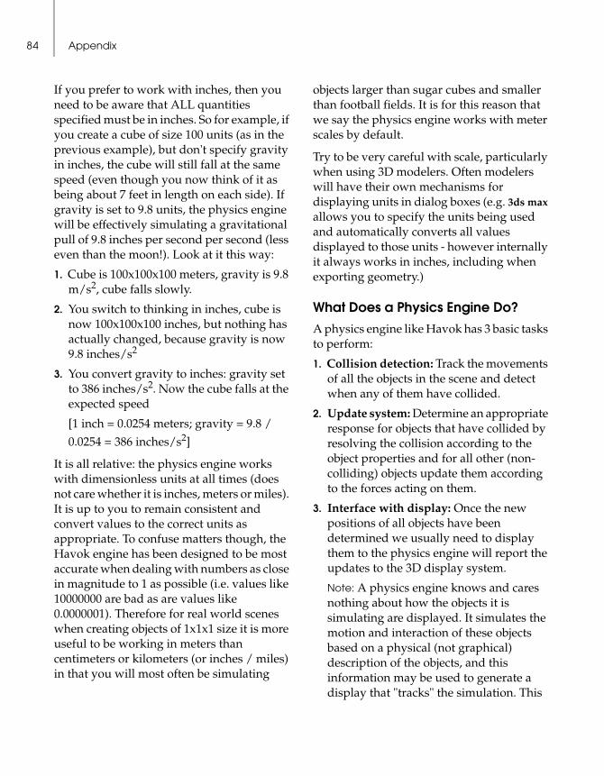
Appendix84
If you prefer to work with inches, then you need to be aware that ALL quantities specified must be in inches. So for example, if you create a cube of size 100 units (as in the previous example), but don't specify gravity in inches, the cube will still fall at the same speed (even though you now think of it as being about 7 feet in length on each side). If gravity is set to 9.8 units, the physics engine will be effectively simulating a gravitational pull of 9.8 inches per second per second (less even than the moon!). Look at it this way:
1. Cube is 100x100x100 meters, gravity is 9.8 m/s2, cube falls slowly.
2. You switch to thinking in inches, cube is now 100x100x100 inches, but nothing has actually changed, because gravity is now 9.8 inches/s2
3. You convert gravity to inches: gravity set to 386 inches/s2. Now the cube falls at the expected speed
[1 inch = 0.0254 meters; gravity = 9.8 /
0.0254 = 386 inches/s2]
It is all relative: the physics engine works with dimensionless units at all times (does not care whether it is inches, meters or miles). It is up to you to remain consistent and convert values to the correct units as appropriate. To confuse matters though, the Havok engine has been designed to be most accurate when dealing with numbers as close in magnitude to 1 as possible (i.e. values like 10000000 are bad as are values like 0.0000001). Therefore for real world scenes when creating objects of 1x1x1 size it is more useful to be working in meters than centimeters or kilometers (or inches / miles) in that you will most often be simulating
objects larger than sugar cubes and smaller than football fields. It is for this reason that we say the physics engine works with meter scales by default.
Try to be very careful with scale, particularly when using 3D modelers. Often modelers will have their own mechanisms for displaying units in dialog boxes (e.g. 3ds max allows you to specify the units being used and automatically converts all values displayed to those units - however internally it always works in inches, including when exporting geometry.)
What Does a Physics Engine Do?A physics engine like Havok has 3 basic tasks to perform:
1. Collision detection: Track the movements of all the objects in the scene and detect when any of them have collided.
2. Update system: Determine an appropriate response for objects that have collided by resolving the collision according to the object properties and for all other (non-colliding) objects update them according to the forces acting on them.
3. Interface with display: Once the new positions of all objects have been determined we usually need to display them to the physics engine will report the updates to the 3D display system.
Note: A physics engine knows and cares nothing about how the objects it is simulating are displayed. It simulates the motion and interaction of these objects based on a physical (not graphical) description of the objects, and this information may be used to generate a display that "tracks" the simulation. This
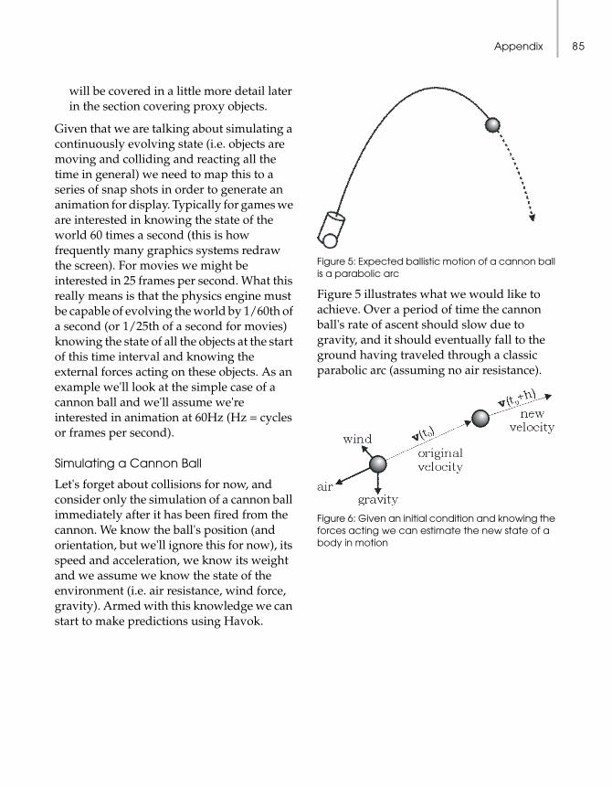
Appendix 85
will be covered in a little more detail later in the section covering proxy objects.
Given that we are talking about simulating a continuously evolving state (i.e. objects are moving and colliding and reacting all the time in general) we need to map this to a series of snap shots in order to generate an animation for display. Typically for games we are interested in knowing the state of the world 60 times a second (this is how frequently many graphics systems redraw the screen). For movies we might be interested in 25 frames per second. What this really means is that the physics engine must be capable of evolving the world by 1/60th of a second (or 1/25th of a second for movies) knowing the state of all the objects at the start of this time interval and knowing the external forces acting on these objects. As an example we'll look at the simple case of a cannon ball and we'll assume we're interested in animation at 60Hz (Hz = cycles or frames per second).
Simulating a Cannon Ball
Let's forget about collisions for now, and consider only the simulation of a cannon ball immediately after it has been fired from the cannon. We know the ball's position (and orientation, but we'll ignore this for now), its speed and acceleration, we know its weight and we assume we know the state of the environment (i.e. air resistance, wind force, gravity). Armed with this knowledge we can start to make predictions using Havok.
Figure 5: Expected ballistic motion of a cannon ball is a parabolic arc
Figure 5 illustrates what we would like to achieve. Over a period of time the cannon ball's rate of ascent should slow due to gravity, and it should eventually fall to the ground having traveled through a classic parabolic arc (assuming no air resistance).
Figure 6: Given an initial condition and knowing the forces acting we can estimate the new state of a body in motion
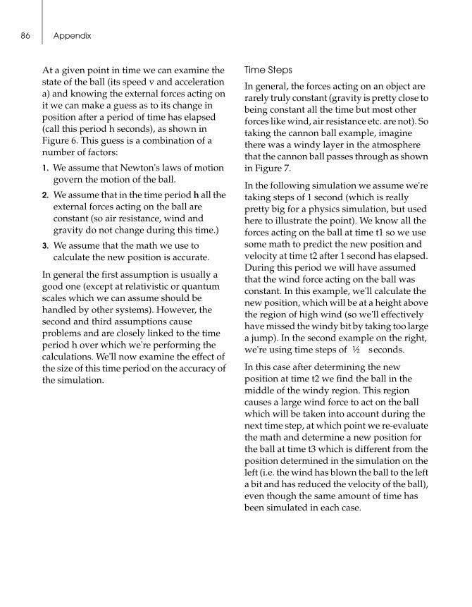
Appendix86
At a given point in time we can examine the state of the ball (its speed v and acceleration a) and knowing the external forces acting on it we can make a guess as to its change in position after a period of time has elapsed (call this period h seconds), as shown in Figure 6. This guess is a combination of a number of factors:
1. We assume that Newton's laws of motion govern the motion of the ball.
2. We assume that in the time period h all the external forces acting on the ball are constant (so air resistance, wind and gravity do not change during this time.)
3. We assume that the math we use to calculate the new position is accurate.
In general the first assumption is usually a good one (except at relativistic or quantum scales which we can assume should be handled by other systems). However, the second and third assumptions cause problems and are closely linked to the time period h over which we're performing the calculations. We'll now examine the effect of the size of this time period on the accuracy of the simulation.
Time Steps
In general, the forces acting on an object are rarely truly constant (gravity is pretty close to being constant all the time but most other forces like wind, air resistance etc. are not). So taking the cannon ball example, imagine there was a windy layer in the atmosphere that the cannon ball passes through as shown in Figure 7.
In the following simulation we assume we're taking steps of 1 second (which is really pretty big for a physics simulation, but used here to illustrate the point). We know all the forces acting on the ball at time t1 so we use some math to predict the new position and velocity at time t2 after 1 second has elapsed. During this period we will have assumed that the wind force acting on the ball was constant. In this example, we'll calculate the new position, which will be at a height above the region of high wind (so we'll effectively have missed the windy bit by taking too large a jump). In the second example on the right, we're using time steps of ½ seconds.
In this case after determining the new position at time t2 we find the ball in the middle of the windy region. This region causes a large wind force to act on the ball which will be taken into account during the next time step, at which point we re-evaluate the math and determine a new position for the ball at time t3 which is different from the position determined in the simulation on the left (i.e. the wind has blown the ball to the left a bit and has reduced the velocity of the ball), even though the same amount of time has been simulated in each case.

Appendix 87
Figure 7: Effects of differing time steps on simulation outcome, the big problem being the assumption of constant force acting on the object during the time period
In general, the smaller the time step taken, the more accurate the result at the end of the time step - so if you want to step forward in time by a large time step t it is better to split this into n steps of a smaller time interval t/n.
This is also true of the math. As the simulation becomes more complex the math required to calculate the new positions and velocities of objects in a simulation also becomes more complex, and as a result the guesses produced by the math give less and less accurate results.
Figure 8: Evolution of a physics system captured in a series of "snapshots"
So the principle is to take small time steps, evaluate all the forces acting on the objects, determine the new positions and velocities (and other parameters) of the objects at the end of the time steps and then start over. What we end up with is a series of snapshots of the state of the system as it evolves as shown in Figure 8.
Integrators
As mentioned earlier, the math becomes less accurate as larger time steps are used. The physics engine implements a fast numerical integration of a series of differential equations describing the motion of objects. An integrator is an algorithm that attempts to estimate the new state of a variable or parameter (e.g. position) knowing information like the rate of change of the parameter (e.g. velocity). There are various

Appendix88
different integrators available. They vary in CPU load and accuracy of result. The following table gives an overview of the integrators provided with the Havok engine:Table 2: integrators and their properties
As can be seen the higher the accuracy required the more CPU power required. We've found that for movie production you are better off with an accurate integrator (like RK45) and taking small time steps, but for real-time performance you should usually start with Euler, the fastest but least accurate, and only move to a more accurate integrator if you are not happy with the accuracy. Later we will talk more about integrators and in particular their effect on stability in constrained systems.
The Simulation LoopWe'll examine now the structure of the physical simulation (shown in Figure 9) and how we integrate this with a 3D display.
Having set up the initial conditions for a given scene, we begin the main simulation loop which basically steps through 3 phases:
1. Detect Collisions: at each step we need to determine which objects have collided. These will result in new collision forces and friction forces being introduced into the system.
2. We then update all the forces acting on the objects either as a result of collision
detection or as a result of input from outside the simulation (here is where we would add input from a user in a real-time game e.g. the user presses the accelerate key should cause the vehicle being driven to accelerate).
Figure 9: the structure of a physics simulation system
3. Having accumulated all the forces we then, using the selected integrator, determine the new state of the objects (position, orientation, velocity, acceleration etc.). This information is then used to update the 3D display.
4. Advance time by the step size h and determine if these new positions have resulted in collisions between any of the objects.
This assumes that at each step in the simulation we actually want to update the display. The next section deals with what happens when this is not the case.
Substeps
Assume we absolutely need to update the display once every 1/60th of a second (i.e. we are either playing a real-time game that refreshes the screen at 60Hz. or we are creating a movie to be played back at 60
Integrator CPU load Accuracy
Euler low low
Midpoint medium medium
Runga Kutta (RK45)
high high
Back Euler medium medium-high

Appendix 89
frames per second.) Ignoring the load on the CPU, this effectively means that we want to step the physics engine at intervals of 1/60th of a second. In many cases this does not present a problem, but if, hypothetically, the accuracy of the simulation was not sufficient (remember: smaller time steps mean better accuracy) then we'd like to decrease the time step even further, let's say to 1/120th of a second. But this would mean we generate twice the number of images we are interested in, which is wasteful. To get around this, the Havok engine allows you to specify the number of substeps to take.
The substep parameter specifies the number of steps the physics engine takes before updating the 3D display. This gives control over the granularity of the physics simulation independent of the display update frequency. So if substeps = 0, then no physics steps are taken. With substeps = 1, a single simulation step is used for each update to the 3D display. With substeps = 2, 2 physics steps are taken, and then the display is updated.
In Figure 10 we have specified that the physics simulation should step at intervals of 1/240th of a second, but that we only update the display once every 1/60th of a second. This has been achieved by instructing the physics engine to employ 4 substeps. Therefore for every 4 steps we update the display only once. By setting the number of substeps we can control the accuracy of the physical simulation independent of the display.
Lower Limit on CPU
An unfortunate but unavoidable side effect of using a physics simulation is that there is a definite lower limit on the CPU time you can give to the physics. In contrast, there's no real lower limit on the CPU time given to graphical display (let's assume you don't have hardware acceleration). As you decrease the CPU allocation to the display you can simply draw fewer polygons, or remove fogging, or turn off lighting, but at no time will the display actually "break".
Figure 10: Substeps allow simulation frequency to be decoupled from display frequency
Physics is different. A physical simulation must be maintained at a stable state (given that each simulation result depends completely on the previous simulation step). If, in one step, we produce a very inaccurate result, then the next step is likely to be even more inaccurate, and you end up in a spiral of decreasing accuracy until eventually the results are garbage (the simulation is said to
Appendix90
have "exploded"). Therefore you can't simply reduce the number of objects or turn off friction to compensate for a reduction in the available CPU resources - you simply have to ensure that your scene can be simulated stably even with the lowest expected CPU bandwidth.
Energy Management
One of the major factors determining the load on the CPU in a physical simulation is the number of objects that are active or moving i.e. being physically simulated. In a typical scene a large number of objects are not actually moving at all, and in theory could be ignored until interacted with. Energy management is concerned with determining which objects in a scene are not doing very much and removing these from the physical simulation (known as turning the object off or deactivating the object) until such time as they begin to move again. The important elements of energy management are:
• When should an object be turned off?
• When should an object be turned back on?
Both questions above are tricky to provide a general answer for and typically the correct answer is highly context dependent. Usually objects are deactivated when they haven’t moved much recently, and are reactivated when hit by other moving objects. However, temporarily removing objects from the simulation remains the best single way to reduce the load on the CPU and it is well worth experimenting with the parameters provided by the Havok engine for automated object deactivation.
Collision DetectionThis is possibly the most crucial part of any physics engine. Collision detection typically accounts for over 90% of the CPU time required for a physical simulation. Given that we are interested in large numbers of interacting objects we have a potential explosion in the number of collision tests we need to do. At a worst case, with n objects in a scene we need to guarantee that every possible pair (sometimes called a collision pair) is checked. This requires n(n - 1)/2 tests (for each object n we test with every other object but not itself, (n - 1), giving n(n - 1) tests, but given that a test for A colliding with B is the same as one for B colliding with A we divide by 2). So for 4 objects we need to do 6 tests; for 100 objects we do 4950 tests. This gets expensive pretty quickly. Given that the physics engine needs some detailed information about each collision in order to be able to resolve it correctly, the collision tests themselves are expensive.
There are a number of ways to speed up this process:
1. Reduce the number of collisions that require detailed collision results to be generated (i.e. use a simpler collision test first).
2. Reduce the complexity of the objects being tested for collisions.
3. Reduce the number of objects.
Obviously always try to achieve the third option first. The number of objects active in a given scene is the primary source of CPU load. If objects can be removed this speeds up the simulation. In the case of the reducing complexity, the difficulty in providing

Appendix 91
detailed collision results is directly associated with the complexity of the objects themselves. We'll address this in the next section. Firstly we'll deal with how the Havok system attempts to achieve a reduction in the number of complex collisions.
Multiphase Collision TestingThe Havok system employs a series of collision tests, each getting progressively more complex, but after each test we eliminate as many objects from the test process before moving to the next level. Assume we have a simple test A and a complex test B. Test A is very fast to run but is not very accurate (but as long as it is conservative this is not a problem - a conservative test may return TRUE i.e. there is a collision, when in fact there isn't but will never return FALSE i.e. there is no collision when in fact there is). Test B is slow to run but highly accurate. The process involves:
• First test all objects with test A eliminating those that definitely do not collide, but not necessarily eliminating all non-colliding pairs.
• Then test with test B which will take the reduced number of collision pairs and perform the complex collision test on these.
As an example consider the tests shown in Figure 11. Here we see an example of the first pass of a collision system. In this case we're using bounding boxes or boxes that enclose fully the objects contained within. We test first to see if any of the boxes overlap (this is
a much faster operation than doing full collision testing on arbitrary shapes), and if they do, that collision pair is passed to the next, more complex pass.
Out of the potential list of 6 collision pairs = { AB, AC, AD, BC, BD, CD } we find that only 2 pairs have overlapping boxes = { AB, CD } and therefore only these 2 collision pairs need further testing. This is sometimes called trivial rejection.
Note that although, for example, pair AB has not been trivially rejected, this does not mean that A and B are actually colliding - only that they might be colliding. We do know, however, that A and C definitely do not collide because their bounding boxes do not overlap.
Figure 11: First pass in a collision detection system - attempting to eliminate as many collision pairs as early as possible
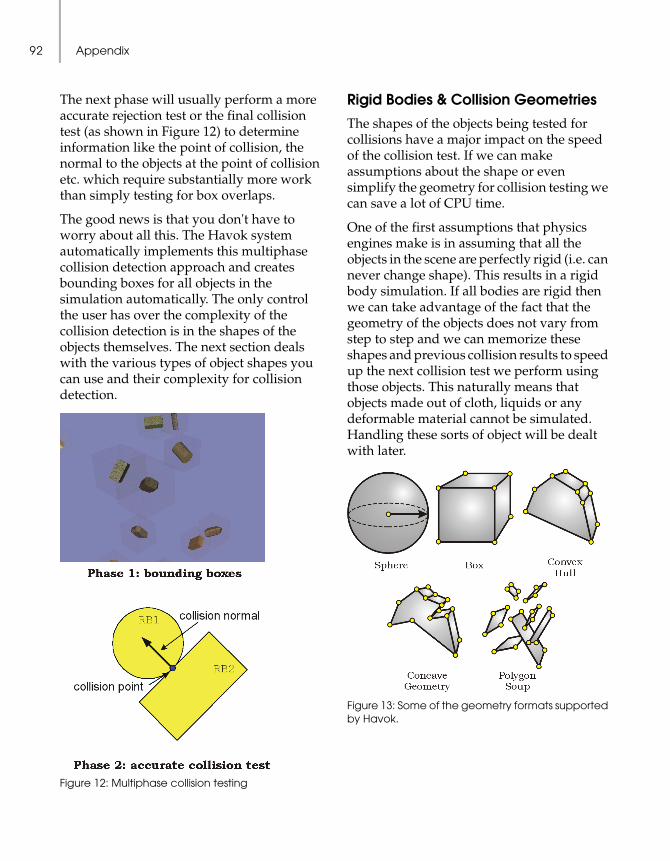
Appendix92
The next phase will usually perform a more accurate rejection test or the final collision test (as shown in Figure 12) to determine information like the point of collision, the normal to the objects at the point of collision etc. which require substantially more work than simply testing for box overlaps.
The good news is that you don't have to worry about all this. The Havok system automatically implements this multiphase collision detection approach and creates bounding boxes for all objects in the simulation automatically. The only control the user has over the complexity of the collision detection is in the shapes of the objects themselves. The next section deals with the various types of object shapes you can use and their complexity for collision detection.
Figure 12: Multiphase collision testing
Rigid Bodies & Collision GeometriesThe shapes of the objects being tested for collisions have a major impact on the speed of the collision test. If we can make assumptions about the shape or even simplify the geometry for collision testing we can save a lot of CPU time.
One of the first assumptions that physics engines make is in assuming that all the objects in the scene are perfectly rigid (i.e. can never change shape). This results in a rigid body simulation. If all bodies are rigid then we can take advantage of the fact that the geometry of the objects does not vary from step to step and we can memorize these shapes and previous collision results to speed up the next collision test we perform using those objects. This naturally means that objects made out of cloth, liquids or any deformable material cannot be simulated. Handling these sorts of object will be dealt with later.
Figure 13: Some of the geometry formats supported by Havok.
Appendix 93
Insisting that all objects are perfectly rigid in a physical simulation is actually pretty bad news for the system (except for collision detection). All colliding objects, no matter how hard, deform even if infinitesimally at the point of contact and then return to their original shape when they bounce away from the collision. When totally rigid objects collide, very large forces are generated in order to keep them apart. This is an unfortunate side effect that needs to be addressed for realistic collisions.
In the Havok physics engine objects are classified according to their shape, and particular shapes have particular properties that make it easier to deal with them during collision detection. The following list classifies object shapes in order of increasing complexity (see Figure 13 for diagrams of some of these):
• Implicit: we have a mathematical representation of the object and base the collision test on this. Implicit objects supported by Havok include:
•spheres
•planes
•polygons
• Polygonal: we have a description of the object in terms of the polygons (usually triangles) making it up. In this case we classify the objects, in order of increasing complexity, as:
•Convex: imagine wrapping the object in a cellophane wrap - if the cellophane touches every part of the surface (i.e. there are no hollows in the surface that the cellophane does not reach) then it's convex. Alternatively, pick a point inside the object and follow an imaginary ray from that point going in any direction out
from the object. If you only pass through the object's surface once, it's convex. Figure 14 depicts some rigid body simulations using entirely convex objects.
•Concave: an object described by a closed surface (no holes or strange self-intersections like Klein bottles). Concave objects are always assumed to represent volumes (i.e. the polygon mesh representing the surface has no holes or gaps in it).
•Polygon Soup: a collection of polygons, not necessarily connected, all grouped and classified as a single object. This is the most expensive format to detect collisions with, but is also the most general.
Figure 14: Rigid body simulations using only convex shapes

Appendix94
In Figure 15, the duck is shown represented as a convex object (the skin defined in the image on the bottom) and the true concave geometry on the top.
Proxy Objects
The good news is that even though an object in a simulation may appear complex, it need not be simulated with this complexity. For example, a car chassis displayed with detailed NURB panels and including wing mirrors and bumpers etc. might be simulated as a box.
This is one of the main ways to reduce the CPU costs of a simulation. These simplified objects representing the more complex display geometry are known as proxy objects or proxy geometries. Artifacts resulting from the use of proxies may be visible and in general you should attempt to make the proxy object as close a fit to the real display geometry as possible
Figure 15: Concave and convex representations of a rubber duck
Figure 16: Collision proxies for a complex shape
In Figure 16 we show a series of proxy objects for a complex geometry (the gray jagged thing which we'll assume is represented as a polygon soup). You can choose any proxy geometry you like for any shape of object but it makes sense to only use a simpler proxy geometry than the actual object itself. In many cases you will actually create a specific geometry (like the last one in Figure 16) that is a combination of a sphere and a box.
The final choice of proxy will represent a tradeoff between speed of collision and accuracy required and is typically very context specific. In Figure 17 the effect of the choice is plainly visible; a sofa geometry (with a pretty high polygon count) is being represented by 2 different proxies, a sphere and a collection of boxes. The collection of boxes is more expensive to compute collisions for but the sphere has a tendency to roll around, so is probably unsuitable in this case.

Appendix 95
Figure 17
In Figure 17, on the left we show a complex sofa object and 2 choices of proxy, on the right we show the simulation in progress (with the proxy objects displayed - although this would normally not be the case). The sphere is less suitable than the collection of boxes.
InterpenetrationObjects in a physical simulation are assumed to be solid and (except in the case of polygon soups) have a defined volume. It makes no sense in the real world to think of one solid object either inside or penetrating another solid object (it's not possible to embed a cup in a table). Similarly in the simulation of the real world, a physics engine is intolerant of objects that are interpenetrating. It also causes disbelief on the part of the viewer of the simulation - we don't expect solid objects to pass through each other. Therefore, a lot of the work performed by the physics engine is to attempt to prevent interpenetrations. This can be pretty tough, particularly when there are large numbers of objects stacked up all pushing downwards under the force of gravity (it's nearly as if they wanted to interpenetrate most of the time!)
When Havok encounters a pair of interpenetrating objects it simply ignores that collision pair and does not attempt to do anything clever - it will always try to prevent it happening in the first place of course. Interpenetrations occur most frequently in the following cases:
• When large forces are acting on objects forcing them to penetrate another object close by (often caused in large stacks).
• If the time step is too large, objects can become embedded in other objects before the physics engine has a chance to do anything about it.
• If the user sets the position of a physical object in such a way as to cause an interpenetration (see next sections for more details).
• If the collision tolerance is too small. See the next sections for more information on this.
The time step used in a simulation has a large impact on the collision detection engine's ability to accurately detect collisions. If large time steps are being taken 2 things can go wrong:
Figure 18 shows large time step issues in collision detection: on the left a collision is missed completely, on the right an interpenetration result.
Figure 18
Appendix96
• Collisions are missed - the so-called "bullet through paper" effect (see Figure 18.) Objects that are moving quickly will pass right through thin objects particularly if the time step is too large (i.e. a time t1 the bullet is in front of the piece of paper, but at the next time step, t2, the bullet has been placed on the other side of the piece of paper.)
• Interpenetration: the time scale is so large that objects become embedded in each other from one time step to the next - too deeply for the physics engine to be able to recover gracefully.
In general there is not much you can do except decrease the time step. For interpenetrations this will often help, but for the "bullet through paper" effect this will usually not solve the problem. Try to avoid very thin objects and extremely fast moving objects.
Inside & Outside
One major consequence of the assumption of solidity and the problems of interpenetration is that you cannot consider most objects to be hollow. A common mistake is to create a box for a room and begin to place objects within the box, thinking these are being placed inside the room. A box, by default, is a solid geometry and any objects placed inside will be tagged as interpenetrating and will likely simply fall through the base of the box if simulated (i.e. collisions between the box and the objects will have been disabled by the physics engine).
A way around this is to represent the box using a polygon soup geometry (unconnected triangles). This will have the desired effect.
Set Position & Deforming GeometryPhysics engines like to control the scene completely. By this we mean the physics engine is carefully storing the state of all objects in the scene and updating this state from frame to frame. If some external system then makes some changes to the scene the physics engine needs to update its state accordingly. This is often fine except when the changes made to the scene actually violate the simulation stability that the physics engine has been attempting to maintain.
Two good examples of this are users setting object positions or orientations (sometimes called object warping) and deforming meshes. Taking the first example it's easy to see how arbitrarily setting the position of an object in the physics scene may cause problems:
• If the object is moved to a position that causes an interpenetration; without additional information the physics engine will simply have to turn off collisions between the moved object and the object it has been moved into.
• If other objects are resting or stacked above the object that is moved; hopefully the stack will simply restructure to fill the gap made by the moved object.
• If other objects are attached to the moved object by springs or constraints: this is the worst case. By moving the object abruptly, the connections to the other objects are

Appendix 97
stretched instantaneously and can cause the system to explode.
Objects may be moved outside of the control of the physics system if they are being keyframed in some way. For such objects, the Havok system needs to be informed that these objects can be expected to move unexpectedly - Havok will track these objects specifically and will attempt to resolve the situation, though not always successfully. In general try to avoid direct manipulation of objects. It is always better to apply forces and impulses (either linear or angular) to the objects to "push" them towards the desired goal.
The case of deforming meshes is subtler, but is related to the difficultly in handling warping objects. An example of this is shown in Figure 19.
Figure 19 shows deforming objects like the squished sphere need to be treated with care in a physics engine. The desired result is shown on the bottom, i.e. the blocks are pushed out of the way when the sphere bulges out.
In this example, a sphere has been keyframed to squash (perhaps to simulate the effect of being squashed from above - note we are talking about keyframing here and not a soft object under physics control). Under normal circumstances this results in an interpenetration.
The sphere's sides bulge out as it deforms into an ellipsoid shape, but this happens outside the control of the physics engine and therefore appears to happen instantaneously. This sort of thing can happen quite often, particularly in situations where meshes are
being generated automatically (e.g. in character animation a skin mesh around a set of bones deforms based on the position of the bones).
Figure 19
The correct result would involve the physics engine tracking the shape of the deforming mesh and when it spots a change in the mesh in a given time step it will use this with the shape of the mesh in the previous step (which it has remembered) to try and figure out how
Appendix98
the surrounding affected objects should move. In this case, the deforming mesh will cause the two blocks on either side to be pushed outwards away from the sphere. The Havok system needs to be told that an object's geometry may deform outside of its control in order to achieve this result.
Figure 20: Object collision are usually only detectable after they have occurred
Collision ToleranceOne final but crucial feature of the Havok system is its implementation of collision tolerances. If you consider the previous sections on collisions and interpenetration you may have spotted that it's pretty hard for the physics engine to detect a collision without an interpenetration having taken place. Because the physics system is based on discrete time steps (of say 1/60th of a second) it is rare that a collision at a given time step will take place where 2 objects are just touching (i.e. a single point of contact).
In Figure 20 this situation is illustrated. 2 spheres are traveling towards each other. At time steps t1 and t2 they are still apart, but at time t3 they have interpenetrated. To avoid this the Havok engine uses a system of collision tolerances. These are minimum distance values that specify how close objects can be before they are deemed to have collided. Consider the collision tolerance to be a "skin" of a certain thickness around the objects. If the skins overlap (or interpenetrate) the objects are said to have collided and the nearest points on the 2 objects are used as collision points.
Figure 21 shows what happens when collision tolerances are used. In this case the spheres has a small collision tolerance that really means that the spheres have a collision proxy that is another slightly larger sphere. At time t2 each of the spheres has collided with the collision tolerance of the other sphere (note that it is not enough that only

Appendix 99
the tolerances have interpenetrated - one of the spheres must be inside the collision tolerance of the other). The system calculates the collision information, assuming that the objects have collided, and takes the appropriate action.
As expected, with large values of the collision tolerance, you'll begin to notice that the objects are not actually hitting. This is particularly noticeable for objects that are stacked (you'll see gaps between them). In general the tolerance should be around 2% - 10% of the size of the object itself. To remove most of these visual artifacts you should increase the size of the visual geometry by approximately half of the tolerance, or alternatively create a collision proxy that has been reduced in size by half the tolerance value.
Figure 21: Using collision tolerances, you can check to see if the tolerances overlap and if so consider the objects to have collided and take appropriate action.

Appendix100
Setting the Scene
The first stage in any physics simulation is to create the scene. This is slightly different to constructing a 3D scene without physics and is constrained by collision tolerances and requirements of non-interpenetration. If you construct a scene in the normal way you will run into difficulties placing objects so that they are stably resting on other objects without collision problems.
As an example take the case of creating a stack of boxes of height h on the floor. Usually you will place the base of the first box at height 0, the second at height h, the third at height 2h and so on, as shown in Figure 22A. But given the collision tolerance issue mentioned in the previous section there will be problems with this approach.
Figure 22: Creating a stable stack
Depending on the numerical accuracy of the simulation, the faces of neighboring boxes will either be classified as interpenetrating or colliding. If interpenetrating, the boxes will fall through each other - if colliding they will immediately bounce off each other (albeit with very little energy, so you may get lucky). Another approach might be to place the boxes such that the collision tolerances overlap, but the boxes are not actually touching as in Figure 22 B. This can also cause

Appendix 101
problems, because the boxes are liable to settle for a while into a stable state (depending on external forces like gravity etc.)
The best way around this is to use the physics engine itself. As shown in Figure 22 C, you should create the boxes initially separated by a distance of more than the collision tolerance. Now simply simulate the scene for a period of time; the boxes will fall the small distance and will settle into a stable stack. Eventually they will turn off as the energy management system kicks in. Now you have a stable stack that is turned off and ready to be saved. Store the positions of the boxes - now you can use these positions to create your stack at a later point in time (making sure to turn the boxes off manually to fully recreate the state of the stack.) You are guaranteed that when the new simulation starts the stack will be stable and unmoving.
Physical Units and ValuesWe've already dealt with the issue of scale and switching between units of measurement. Physics engines are not simply concerned with lengths and weights however - in fact there is a very large number of different measures in use at any given time. In this section we'll list some of these and give the units used to quantify them. Despite the apparent complexity of dealing with all these units, in many cases you will not need to worry: we find that experimentation with values is ultimately the best way to proceed when designing a scene.
It is often useful, however, to fall back on an analysis of the scene and units used to at least determine the ballpark values required to achieve a desired goal.
For simplicity we'll stick with the metric system in the following sections:
• m = meters
• kg = kilograms
• s = seconds
• N = Newtons (measurement of force: 1 N = force required to change the speed of a 1kg object by 1 m/s in 1 s).
• rad = radians (1 rad = 180/p degrees where p = 3.14159… ).
Note: Some implementations of the Havok physics technology use degrees as units of angle. This will be clearly stated in the accompanying documentation.
To read the units detailed below, apply the following conventions:
• nx/y = x per y e.g. m/s = meters per second (i.e. velocity or speed). Note that x/y is sometimes written as x y-1.
• nx/y2 = x per y squared or x per y per y e.g. m/s2 = meters per second squared or meters per second per second (i.e. acceleration)
Position Based
Position (m)
A better description of this term is displacement or distance.
Velocity (m/s)
Speed - how fast is an object traveling relative to some frame of reference.
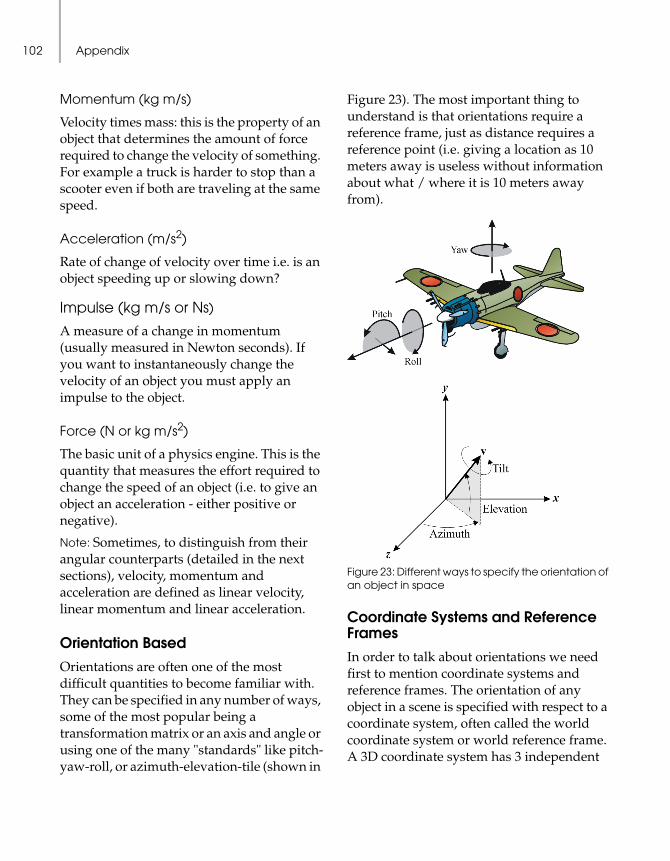
Appendix102
Momentum (kg m/s)
Velocity times mass: this is the property of an object that determines the amount of force required to change the velocity of something. For example a truck is harder to stop than a scooter even if both are traveling at the same speed.
Acceleration (m/s2)
Rate of change of velocity over time i.e. is an object speeding up or slowing down?
Impulse (kg m/s or Ns)
A measure of a change in momentum (usually measured in Newton seconds). If you want to instantaneously change the velocity of an object you must apply an impulse to the object.
Force (N or kg m/s2)
The basic unit of a physics engine. This is the quantity that measures the effort required to change the speed of an object (i.e. to give an object an acceleration - either positive or negative).
Note: Sometimes, to distinguish from their angular counterparts (detailed in the next sections), velocity, momentum and acceleration are defined as linear velocity, linear momentum and linear acceleration.
Orientation BasedOrientations are often one of the most difficult quantities to become familiar with. They can be specified in any number of ways, some of the most popular being a transformation matrix or an axis and angle or using one of the many "standards" like pitch-yaw-roll, or azimuth-elevation-tile (shown in
Figure 23). The most important thing to understand is that orientations require a reference frame, just as distance requires a reference point (i.e. giving a location as 10 meters away is useless without information about what / where it is 10 meters away from).
Figure 23: Different ways to specify the orientation of an object in space
Coordinate Systems and Reference FramesIn order to talk about orientations we need first to mention coordinate systems and reference frames. The orientation of any object in a scene is specified with respect to a coordinate system, often called the world coordinate system or world reference frame. A 3D coordinate system has 3 independent
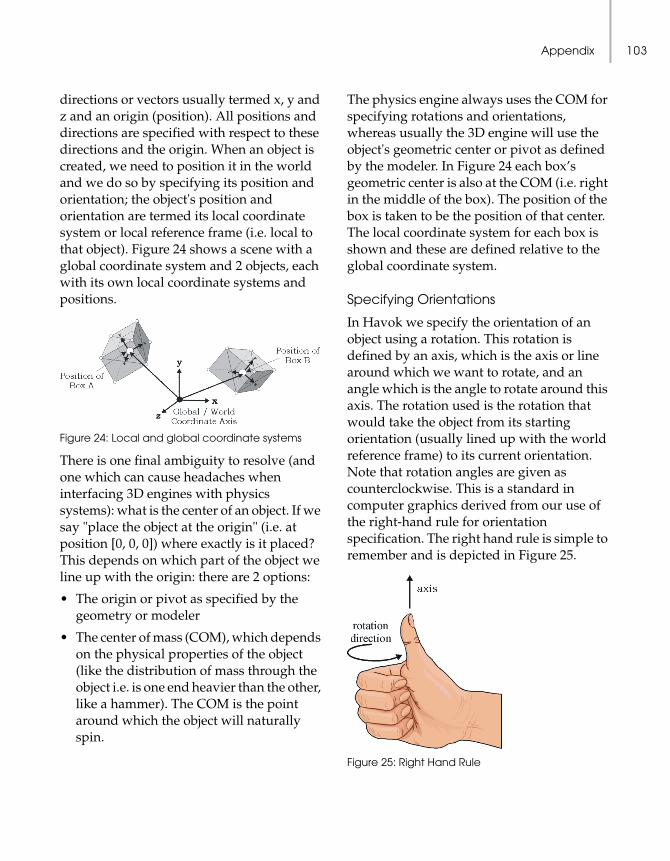
Appendix 103
directions or vectors usually termed x, y and z and an origin (position). All positions and directions are specified with respect to these directions and the origin. When an object is created, we need to position it in the world and we do so by specifying its position and orientation; the object's position and orientation are termed its local coordinate system or local reference frame (i.e. local to that object). Figure 24 shows a scene with a global coordinate system and 2 objects, each with its own local coordinate systems and positions.
Figure 24: Local and global coordinate systems
There is one final ambiguity to resolve (and one which can cause headaches when interfacing 3D engines with physics systems): what is the center of an object. If we say "place the object at the origin" (i.e. at position [0, 0, 0]) where exactly is it placed? This depends on which part of the object we line up with the origin: there are 2 options:
• The origin or pivot as specified by the geometry or modeler
• The center of mass (COM), which depends on the physical properties of the object (like the distribution of mass through the object i.e. is one end heavier than the other, like a hammer). The COM is the point around which the object will naturally spin.
The physics engine always uses the COM for specifying rotations and orientations, whereas usually the 3D engine will use the object's geometric center or pivot as defined by the modeler. In Figure 24 each box’s geometric center is also at the COM (i.e. right in the middle of the box). The position of the box is taken to be the position of that center. The local coordinate system for each box is shown and these are defined relative to the global coordinate system.
Specifying Orientations
In Havok we specify the orientation of an object using a rotation. This rotation is defined by an axis, which is the axis or line around which we want to rotate, and an angle which is the angle to rotate around this axis. The rotation used is the rotation that would take the object from its starting orientation (usually lined up with the world reference frame) to its current orientation. Note that rotation angles are given as counterclockwise. This is a standard in computer graphics derived from our use of the right-hand rule for orientation specification. The right hand rule is simple to remember and is depicted in Figure 25.
Figure 25: Right Hand Rule
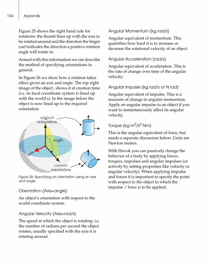
Appendix104
Figure 25 shows the right hand rule for rotations: the thumb lines up with the axis to be rotated around and the direction the finger curl indicates the direction a positive rotation angle will rotate in.
Armed with this information we can describe the method of specifying orientations in general.
In Figure 26 we show how a rotation takes effect given an axis and angle. The top right image of the object , shows it at creation time (i.e. its local coordinate system is lined up with the world's). In the image below the object is now lined up to the required orientation
Figure 26: Specifying an orientation using an axis and angle
Orientation (Axis+angle)
An object’s orientation with respect to the world coordinate system.
Angular Velocity (Axis+rad/s)
The speed at which the object is rotating: i.e. the number of radians per second the object rotates, usually specified with the axis it is rotating around.
Angular Momentum (kg rad/s)
Angular equivalent of momentum. This quantifies how hard it is to increase or decrease the rotational velocity of an object.
Angular Acceleration (rad/s)
Angular equivalent of acceleration. This is the rate of change over time of the angular velocity.
Angular Impulse (kg rad/s or N rad)
Angular equivalent of impulse. This is a measure of change in angular momentum. Apply an angular impulse to an object if you want to instantaneously affect its angular velocity.
Torque (kg m2/s2 Nm)
This is the angular equivalent of force, but needs a separate discussion below. Units are Newton meters.
With Havok you can passively change the behavior of a body by applying forces, torques, impulses and angular impulses (or actively by setting properties like velocity or angular velocity). When applying impulse and forces it is important to specify the point with respect to the object to which the impulse / force is to be applied.
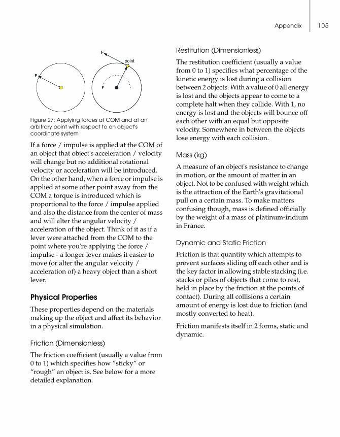
Appendix 105
Figure 27: Applying forces at COM and at an arbitrary point with respect to an object's coordinate system
If a force / impulse is applied at the COM of an object that object's acceleration / velocity will change but no additional rotational velocity or acceleration will be introduced. On the other hand, when a force or impulse is applied at some other point away from the COM a torque is introduced which is proportional to the force / impulse applied and also the distance from the center of mass and will alter the angular velocity / acceleration of the object. Think of it as if a lever were attached from the COM to the point where you're applying the force / impulse - a longer lever makes it easier to move (or alter the angular velocity / acceleration of) a heavy object than a short lever.
Physical PropertiesThese properties depend on the materials making up the object and affect its behavior in a physical simulation.
Friction (Dimensionless)
The friction coefficient (usually a value from 0 to 1) which specifies how “sticky” or “rough” an object is. See below for a more detailed explanation.
Restitution (Dimensionless)
The restitution coefficient (usually a value from 0 to 1) specifies what percentage of the kinetic energy is lost during a collision between 2 objects. With a value of 0 all energy is lost and the objects appear to come to a complete halt when they collide. With 1, no energy is lost and the objects will bounce off each other with an equal but opposite velocity. Somewhere in between the objects lose energy with each collision.
Mass (kg)
A measure of an object's resistance to change in motion, or the amount of matter in an object. Not to be confused with weight which is the attraction of the Earth's gravitational pull on a certain mass. To make matters confusing though, mass is defined officially by the weight of a mass of platinum-iridium in France.
Dynamic and Static Friction
Friction is that quantity which attempts to prevent surfaces sliding off each other and is the key factor in allowing stable stacking (i.e. stacks or piles of objects that come to rest, held in place by the friction at the points of contact). During all collisions a certain amount of energy is lost due to friction (and mostly converted to heat).
Friction manifests itself in 2 forms, static and dynamic.

Appendix106
Figure 28: Static and dynamic friction in action.
The boulder is held in place by static friction until enough force is applied to break the contact (i.e. the plank has been raised to a sufficient height), after which the boulder begins to slide and dynamic friction kicks in which acts against the sliding action, generating heat.
Figure 28 gives an example of static and dynamic friction in action. In Havok you set a single friction coefficient value and the engine manages the transition between the friction modes for you.
Next StepsWe've briefly covered most of the main topics of physical simulation. This is a very rich subject matter and there's certainly a lot more to know but this should be sufficient to help you understand Havok documentation, whether for reactor™ or other Havok products. We have specifically not attempted to cover all areas of the Havok physics technology but have focused instead on the general principles that underpin all simulation. We'll briefly describe now some of these other physics technologies available from the Havok engine.
Figure 29: Constrained systems in action
Constrained DynamicsIn many cases we want to construct physics systems that have constraints or attachments between sub parts of a larger assembly. There are many types of constraint and some of those provided by Havok include:
• Springs: Forces are applied to objects connected by springs to attempt to keep the objects within a desired distance from each other (the rest length).
• Dashpots: Stiff springs.
• Reduced coordinate systems: Systems of rigid bodies are not simulated independently but are simulated as a large system all at the same time. Some reduced coordinate constraints include hinges, ball and socket joints, prismatic joints and universal joints.

Appendix 107
Constraints are a requirement for creating any dynamic system like a car chassis, or a locomotive engine. Forces applied to one object are instantaneously applied to all objects connected to this one, so when the piston on a locomotive pushes forward, the wheels begin to spin. See Figure 29 for some examples of constrained systems.
The fan blade is connected to the base via a revolute joint and the water machine on the right uses a series of constraints to create the water powered block pushing mechanism.
Non Rigid Body DynamicsSo far we have been assuming that all objects are rigid (i.e. the geometry or shape does not change during the simulation). In order to simulation soft, cloth, rope or liquid objects we need to lift this restriction. Most of what has been discussed earlier still applies except for the details of collision detection. For deformable objects, collision detection becomes much more difficult - given that the object can change shape dramatically between time steps and also can attempt to collide with itself (this is particularly true of cloth, where interpenetration prevention is very expensive).
Some examples of deformable surfaces are shown in Figure 30.
Figure 30: Examples of deformable objects
Figure 30 shows (a) lots of cloth and rope elements used in a scene (courtesy of Blizzard Entertainment) (b) a piece of cloth slides over a mannequin's head (c) blobby objects land on a hard surface (d) a water pool simulation with floating raft and rubber duck.

Appendix108
Analyze WorldThe Analyze World function alerts you if you are using unusual values in your scene. For example, if your scene has a very high gravity setting or uses large objects with a very small mass, the Analyze World function detects these values and notifies you. The Analyze World button is located in the Advanced rollout.
Angular DashpotAn angular dashpot is a type of dashpot that attempts to force objects to maintain their initial relative orientations. If you rotate one, a turning force is applied to both to try to equalize their orientations. Dashpots are highly damped springs. Use them to constrain the movement of objects with reference to a point, or to another object.
Animation RolloutThe Animation rollout contains the basic animation parameters. Use the Animation rollout to specify the start and end frames for creating 3ds max™ keyframes, as well as the number of frames per second.
Bounding BoxA bounding box is an enclosing box that surrounds an object in order to give it a convex geometry. Using a bounding box, you can give a convex geometry to an object that is displayed as concave. The Use Bounding Box option is displayed in the Properties rollout.
Bounding SphereA bounding sphere is an enclosing sphere that surrounds an object in order to give it a spherical geometry. The object is then treated as a perfect sphere that contains its original geometry. The Use Bounding Sphere option is displayed in the Properties rollout.
CameraThe Camera button in the Display rollout enables you to select a camera as the display camera. The scene in the reactor™ display window is viewed from the selected camera. If you do not set a camera, reactor uses the default starting camera.
Glossary110
ClothA two-dimensional mesh of triangles used for objects such as fabrics, cloaks, sheets of metal, and other flat or folding bodies.
Cloth CollectionThe term used to describe a set of cloth objects. Cloth must be added to a collection, so that they be can be solved for simulations.
Collision ToleranceCollision tolerance is the value below which objects collide in a simulation. Higher collision tolerance values usually mean more stable simulations. A balance must be struck between stability and visual effect. The Collision Tolerance option is located in the Advanced rollout.
Command PanelA command panel displays a collection of related buttons and fields. It has an identifying tab at the top to enable easy selection. Command panels contain rollouts, which lead to sub groups of related buttons and fields. 3ds max has six command panels. These are: Create, Modify, Hierarchy, Motion, Display and Utilities.
Compound Rigid BodiesCompound rigid bodies are rigid bodies composed of more than one primitive. To construct a compound rigid body, use the 3ds max function to group together a number of primitives. Compound rigid bodies are useful if the density of the object you want to model is not uniform or if the object is concave but can be easily decomposed into several convex primitives.
ConcaveA concave object is any object that does not pass a Convexity Test. Most objects in the real world are concave. Concave objects can have holes, cavities, or non-closed geometries. Concave objects include spirals, teapots, and sinks.
ConvexObjects are convex if, given any two points inside the body, you can always go in a straight line from one to the other without going out of the body. Convex objects include cylinders, spheres, and boxes.
DampingDamping means reducing the energy of a spring or a soft body so that its fluctuations in shape reduce with each oscillation.
DashpotA dashpot is a special type of highly damped spring. You can use dashpots to constrain the movement of objects.
DensityFor fluids, this describes how dense the fluid is with respect to water(Relative density). For instance light oil would have a density of about0.7. Density determines whether an object will float or sink in a fluid. An object's density is automatically calculated using its volume and mass. Cloth uses a property called Buoyancy to determine its density, as it has no volume.

Glossary 111
Deformable MeshA deformable mesh is a special type of object that you can use as a skin. For example, you could use one as the skin of a character. Deformable meshes work on a kind of skin-and-bones basis, where the mesh forms the skin and several rigid bodies form the bones.
Deformable Mesh CollectionA deformable mesh collection (created using the DMCollection option) is a collection for deformable objects, which enables you to assign different solvers to determine their movement in a simulation.
DeactivatorYou can use a deactivator to tell the engine to remove an object from a simulation once its energy level has dropped to specified level.
DisplayThe Display rollout contains the basic parameters that control the reactor preview simulation. You use the Display rollout to select the appropriate camera and lights, and to select the texture quality of the preview.
Display ProxyIn the Properties rollout, you can associate an object with another object. In a simulation, the associated object is displayed in place of the original object. Display Proxy is the term used to describe the associated object.
Dynamic FrictionDynamic friction refers to the friction associated with a moving object. It is a measure of the resistance between two objects rubbing against each other.
ElasticityThe elasticity coefficient of a rigid body is the factor that determines the ratio of a body's speed before and after a collision.
Entity CollectionEntities are the main components of a simulation and are grouped into entity collections. A rigid body collection is an example of an entity collection.
Freeform DeformationFreeform deformation (FFD) is a tool that you can use to encase a soft object in a simple mesh. This mesh then governs the movement and reactions of the soft object, which gives you greater speed in resolving their reactions.
FrictionFriction is the resistance of one surface to another that moves over it. It is the force that makes it difficult for one object to slide along the surface of another. reactor enables you to specify the friction associated with an object.
LightsSelect lights using the Lights section in the Display rollout. If you do not select any lights, a default light is used from the same position as the camera. You can add up to six lights to a simulation.
Glossary112
Linear DashpotLinear dashpots are highly dampened springs. You use them to constrain the movement of objects with reference to a point or another object.
Mass Mass is a property of all reactor bodies. Single primitives can have a mass, as can compound bodies. Compound bodies are the only bodies that can have unevenly distributed mass.
MeshThe Use Mesh function stipulates that the actual mesh of an object should be used for simulation.
Mesh Convex HullThe Mesh Convex Hull option is located in the Properties rollout. Use this option to surround a concave object with an invisible wrapping. When you do this, reactor treats the object as convex during simulation.
Mouse SpringIn the reactor display window, you can use the mouse to interact with the simulation. You can right-click on an object and move it to another location. The mouse spring is the virtual spring that exists between the mouse pointer and the object in the scene. If you increase the strength of the spring, it is easier to move objects. Mouse Spring settings are located in the Display rollout.
Optimized Convex HullThe optimized convex hull of an object is typically used for concave objects. The convex hull of an object is optimized for simulation by decreasing the tessellation. The Optimized Convex Hull option is located in the Properties rollout.
Optimized Geometry / MeshOptimized geometries are geometries that have been less highly tessellated in order to speed up simulation or display. The optimization options are located in the Properties rollout. The Optimized Mesh option can be used to substitute the geometry of a convex object with an optimized version of its geometry.
PlaneA plane is a flat surface. The Plane system in the Create command panel inserts a plane. In reactor, in the Helpers you will find another plane. This plane represents a half-space and is infinite. Unlike a standard plane, the reactor plane does not require the specification of a concave mesh.
Preview In WindowThe Preview In Window button enables you to view and interact with your scene in real time within the reactor display window. The Preview In Window button is located in the Display rollout.
Glossary 113
ProxiesProxies are objects whose geometry is used to replace that of another object. You may use a substitute when displaying or simulating a body. For simulation of a body, you may also use the convex hull of a proxy object. The proxy options are located in the Properties rollout.
Proxy Convex HullA Proxy Convex Hull is the convex hull of a proxy simulation object. A body may be simulated using the convex hull of another object. This other object is referred to as the proxy object. To use the proxy convex hull, go to the Simulation Geometry section of the Properties rollout.
Proxy MeshA proxy mesh is a mesh or geometry that can be substituted for the actual geometry of an object during simulation. This proxy object can be concave or convex, regardless of the original body.
Rest LengthRest length is the length of a spring at which there is no force applied to it. A spring will always tend towards its rest length.
Rigid BodyA Rigid Body is one of the most basic types objects. Rigid bodies are literally objects whose shape does not change in a scene. They are commonly used to represent many kinds of objects, from tables and chairs to teapots and rocks.
Rigid Body CollectionA Rigid Body Collection is a specially defined term used to describe a set of rigid or hard objects. Rigid bodies must be added to a collection for reactor to apply solvers to them.
ShadowsYou can view shadows in the reactor display window. Only lights on to a plane can cast shadows.
SimulationA simulation is a preview of your scene or animation. You can preview your scene by clicking the Preview In Window button in the Display rollout. If you make any changes to the properties associated with your animation in the Animation rollout, you must click the Perform Simulation button to re-compile your animation.
Soft BodyA soft body is an object whose shape is deformable in reaction to the impact of forces and other objects in a simulation.
Soft Body CollectionThe term that describes a set of soft or flexible bodies. To include a soft object for solvers it must be added to a Soft Body Collection.
SolverA Solver is a function that calculates the reactions of a body when placed in a simulation. Solvers work on collections of objects, and there are different kinds of solvers available for different kinds of objects.

Glossary114
SpringA spring is an elastic connection between two objects. You use the spring system in reactor to constrain the movements of objects.
Static FrictionStatic friction refers to the friction associated with an object while it is at rest. It is a measure of resistance in response to an external force tending to slide an object over another.
StepsA step is a single reactor simulation step, within which there may be several substeps to increase the accuracy of the simulation. There is a one-to-one mapping between steps and 3ds max keyframes.
StiffnessStiffness is the property of a spring that determines how quickly a spring returns to its rest length. Very high values of stiffness in a spring can cause instability.
SubstepsSubsteps are steps within steps. Increasing the number of substeps in a step improves the precision of an animation.
SystemSystems are constraints that impact upon objects in a simulation. Systems can change the properties of objects and control the relationships between objects.
Test ConvexityThe Test Convexity button in the Properties rollout checks whether an object is convex or not.
Texture QualityTexture quality refers to how detailed the textures used for display are. These can be 256x256, 128x128 or 64x64. The more detailed the textures, the slower a display may run.
Toy CarThe Toy Car is a feature included in reactor that allows you to create cars and other vehicle types quickly and easily.
Unyielding BodiesUnyielding bodies are objects whose keyframed animations are strictly observed within a reactor simulation.
ViscosityFor fluids, this describes how much resistance an object experiences as it tries to move through the fluid. Water is assumed to have a viscosity of 1.0.
World Scale ParameterThe World Scale parameter stores the correspondence between the units you have used in your scene and the units that will be used in the reactor simulation. 3ds max lets you use whatever units you want. When simulating, reactor must know the ratio between 1 unit in 3ds max and 1 meter in the simulation. The World Scale parameter is located in the Advanced rollout.

Symbols.cui file 3
Numerics3D coordinate 1023D display 88, 893D display system 843D engine 1033D modeler 843D scene 1003ds max 4 1, 3, 5, 9, 10, 11, 16, 17, 19, 20, 21, 22, 24, 26, 28,
32, 39, 42, 50, 57, 59, 60, 61, 62, 64, 69, 71, 73, 75, 78,84, 109
internal hierarchy 113ds max 4 hierarchy 73
AAccelerate key 88Acceleration 88, 101, 105Accuracy 60, 78, 79, 80, 81, 86, 88, 89, 94Accuracy of result 88Accurate integrator 88Accurate rejection test 92Accurate simulation 62Action 53
fracture 54, 56motor 54, 56wind 53, 54
Actionsadding 54
Add button 8, 23, 29, 35, 46, 50, 57, 68Add Drag Action 77Adding a deactivator 12Adding lights 9Advanced Parameters 32
Advanced rollout 11, 24, 62, 63, 75, 77, 109, 110, 114Advanced simulation options 77Air resistance 85, 86Aircraft hangar 83Airflow 79Algorithm 87Allow Wheel Penetration 50Analyze before simulation checkbox 78Analyze World 50, 75Analyze World button 78, 109Analyze World function 109Analyze World test 78Analyze World utility 46Ang parameter 77Ang Speed 56Ang. Speed 56Angle 102, 103Angular acceleration 104Angular damping 77Angular dashpot 42, 44, 109Angular impulse 104Angular momentum 104Angular speed 50Angular Strength 51Angular velocity 77, 104Animate button 61Animation 11, 20, 24, 32, 39, 57, 59, 60, 61, 62, 63, 78, 81,
82, 85Animation bar 60, 61Animation playback 82Animation rollout 60, 61, 64, 109, 113Animation section 61Animation Time 64Applies To... section 55Applying a proxy to a group 18
Index116
Applying textures 10Artifact 94, 99Assembly 81Assigning a material 10Atmosphere 86Attach to Rigid Body constraint 48Attach to Rigid Body modifier 45AttachToRB modifier 49Avoid Self-Intersections option 29, 30Axis 102, 103Axis of rotation 47, 56Azimuth-elevation-tile 102
BBack Euler 88Back-Euler 12Background Color menu option 4Ball and socket joint 47, 106Ballistic motion 79Behavior 81Believability 81Bend 30Bind to Space Warp icon 39Blizzard Entertainment 107Body space 44, 56Bone 97Bones 62Boolean compound 60Boulder 106Boundary condition 80boundary condition 80Bounding box 16, 91, 92, 109Bounding Sphere 60Bounding sphere 16, 109Box Faces radio button 25Box overlap 92Break after collision 57Break during collision 57Building a compound rigid body 17Building compound rigid bodies 17Bullet through paper effect 96Buoyancy 27, 29Buoyancy properties 37Buoyancy property 110Butterfly effect 81
CCalculation 79, 86Camera 4, 5, 28, 35, 38, 48, 109
adding 9Camera button 109
Camera Setting menu option 4Cameras
adding 3Cannon ball 85cannon ball 86Canon ball 85Car 49, 50, 80Car chassis 94, 107Car model 41Cast Shadows on Plane option 6Casts shadows checkbox 5Cellophane wrap 93Center of mass 103Centimeter 84Changing scale 83Chaos 81, 82Chaotic behavior 82Character 82Character animation 62, 97Chassis 50Chassis button 50Cheap solver 46CLCollection button 29Closed surface 93Cloth 27, 28, 30, 31, 32, 45, 48, 49, 53, 54, 92, 107, 110
air resistance 29assigning properties 27damping 28deformation 29friction 28intersection 29mass 28physical properties 27relative density 29smooth level 29stiffness 28vertex selection 29
Cloth collection 29, 31, 48, 54, 110adding bodies 29adding objects 27creating 27
Cloth collections 27Cloth dynamics 30Cloth modifier 48Cloth simulation 32Clothing 81Coefficient of friction 23, 28, 35Coefficient of restitution 77Collection 12, 39, 46, 62, 81Collection symbol 23Collections

Index 117
creating 3Collinear creasing 32Collision 57, 62, 68, 84, 88, 90, 93, 94, 95, 96, 98, 99, 100,
105detection 93
Collision detection 26, 50, 76, 84, 88, 90, 92, 93, 95, 107Collision force 88Collision geometry 92Collision pair 90, 91, 95collision point 98Collision proxy 98Collision resolution 76, 77Collision result 92Collision system 91Collision test 92, 93Collision tests 90Collision tolerance 76, 77, 95, 98, 100, 110Collision Tolerance option 110Collisions 24, 49COM 103, 105Command panel 110command panels
Create 73Commands 68Common Local Orientation 50Complex collision 91Complex collision test 91Complex display geometry 94Complex fold stiffness 30, 31Complex force model 30Complex forces 30Complex Friction resolver 77Complex test 91Compound body 54Compound objects 17Compound rigid body 19, 28, 56, 110Compression and expansion 23Computational fluid dynamics 79Computer graphics 103Concave 11, 13, 15, 22, 60, 93, 110Concave geometry 94Concave mesh 22Concave object 13, 17, 19Concave properties rollout 17Confined path 47Conform to Shape button 26Constrain button 73Constrain Deformation 29, 32Constrain IK Chain with Points utility 73Constrained dynamics 106Constrained system 88, 107
Constraint 34, 35, 44, 45, 46, 49, 53, 56, 77, 96, 106, 107AttachToRB 48point-to-nail 45, 47point-to-path 45, 47point-to-point 45, 46solver 45
Constraint model 35Constraint solver 45, 47, 73Constraint strength 56, 73Constraint system 45, 77Constraint systems 41Constraints 41Continuum of simulation 80Convex 11, 15, 60, 93, 110convex 17Convex hull 16, 19Convex object 13Convex segments 17Convexity Test 110Convexity test 14Coordinate system 102, 105Corrective forces 51CPU 89CPU allocation 89CPU bandwidth 90CPU cost 94CPU load 88, 90CPU power 88CPU resources 79, 90CPU time 89, 90Create command panel 42, 43, 112Create menu 35Create panel 8, 23, 38, 47creating 3Creating a cloth 27Creating a scene 3, 8CSolver 46CSolver system 56Current orientation 44Customize menu 3
DDamping 6, 21, 42, 45, 110damping 28Damping coefficient 23, 28, 35Damping parameter 30Dashpot 41, 42, 44, 45, 106, 110
adding 41, 44angular 42, 44consistency 44established points 44

Index118
forces 44linear 42, 44properties 41strength 45zero rest length 42
Deactivate 39Deactivation 90Deactivator 12, 39, 111
Samples option 12Time option 12
deactivator 12Decreasing accuracy 89Define Collision Pairs option 12Defining collision pairs 12Deformable material 92Deformable mesh 111Deformable mesh collection 111Deformable object 107Deformable surfaces 107Deformation 29, 62
scale strength 39Deforming geometry 96Deforming mesh 62, 96, 97
freeze 63Updates/Frame 63
Deforming mesh collection 62Deforming mesh properties 63Degree 101Delaunay checkbox 32Delaunay triangulation 32Delete button 68Delete Keyframes button 63Delete Now button 63Density 17, 39, 50, 110Dialog box 72, 84Differential equation 87Dimensionless 105Dimensionless unit 84Disable All Collisions 62Disabled 12, 51Disabled checkbox 11Disabled list 12Disabling collections 11, 24Discrete event 80Discrete event simulation 80Disk space 63Display 6, 11, 88, 89, 111Display Children option 11, 73Display frame rate 11Display geometry 14, 94display geometry 16
Display menu 4Display Proxy 20Display proxy 11, 18, 20, 111Display rollout 5, 6, 9, 44, 60, 109, 111, 112, 113Display simulation 37display simulation 24Display Subtree option 18Display update frequency 89Display window 3display window 9Distance 31DMCollection button 62DMCollection option 111Do not affect rigid body option 49Documentation 106Drag action 77Dynamic friction 105, 111Dynamic system 107Dynamics simulation 76
EEdges menu option 4Elastic connection 41Elasticity 7, 9, 10, 69, 111Element 54, 68, 79Element based simulation 81Ellipsoid 97Enable Sheltering option 55Enabled 12Enabled list 12End 63End Frame 60, 61, 63Energy 12, 30, 42, 57, 100, 105Energy Loss 57Energy management 90Energy management system 101Energy threshold 24Entities 77Entity 12, 80, 81, 111Entity collection 7, 27, 29, 111Environment 85Euler 12, 88Events 80, 81Evolution 87Example scripts 69Expensive solver 46Exported information 19External force 82, 85, 86, 101
Index 119
FFaces menu option 4Factors 86Fan 54Fan blade 107FFD 24, 25, 61, 111
changing configuration 26FFD (un)selection panel 25FFD animation 61FFD box sides 25FFD mesh 26, 61FFD mesh selection 25FFD modifier 21FFD Soft Bodies Only constraints 49FFD soft body 24FFD-Based button 25Final collision test 92Finger 104Finite element 79Fixed end 33Fixed Step menu option 4Fixing 24Floating toolbar 69Fluids 37Fogging 89Fold stiffness 30, 31Force 56, 81, 84, 86, 88, 95, 97, 101, 104, 105, 106Force models 30Forces 49, 51, 76Fracture 53Fracture action 56, 57Fracture Properties 57Fracture set 54Fracturing body 57Frame 26, 60, 61, 89, 96Frame field 26Frames/Key value 60Free end 33Freeform deformation 24, 111Freeze checkbox 63Frequency 55Friction 7, 9, 10, 17, 21, 69, 90, 105, 111friction 10Friction coefficient 10, 105, 106Friction force 88Friction values 77Function 69
GGain 56Game 81, 82, 85Game scenario 82Gap 93General principle 106General solver 46Generic unit 75Geometric center 103Geometry 26, 84, 92, 94, 96, 98, 103, 107Geometry / Sim Edges option 20Geometry menu 4, 15, 16Geometry proxy 19, 20Get from / Set to Material 10Get From Material 10getUserProp 69Global coordinate system 103Global value 76glossary 109Granularity 89Graphical display 89Graphical representation 37Graphics system 85Gravitational pull 84, 105Gravity 75, 76, 83, 84, 85, 86, 95, 101Gravity menu option 4Grid 79Grid lines 31Group function 17Group menu 18Groups 17
HHardware acceleration 89Havok 81, 83, 85, 95, 97, 103, 104, 106Havok engine 83, 84, 88, 89, 90, 98, 106Havok physics 101, 106Havok physics engine 79, 83, 93Havok physics primer 79Havok products 79Havok system 91, 92, 97, 98Havok technology 79, 106Havok* list 68HavokPerformSimulation 69Heat 105Heat distribution 81Helix Shape 34Help menu 65

Index120
Helpers 23, 112Helpers drop-down menu 8, 42, 43Helpers icon 8, 42, 43Helpers option 23, 25, 35High-end simulation 80Higher accuracy 88Hinge 106HK* list 68HKRBCollection 68Hole 93Hollow 93, 96Hookean spring 42
IIcon Orientation 50Ignore Collisions option 49Ignoring collision 62ignoring collision 48IK chain 71Images 89Impact position 81Implicit 93Impulse 54, 57, 97, 102, 104Inaccurate simulation 63Inch 75, 84inch 76Individual behavior 80Industrial design 79Initial condition 88Initial physical properties 69Initial position 61Initial velocity 61Input 88Integration step 24Integrator 45, 87, 88Integrators 87Interaction 84interaction 84Interface with display 84Internal integration step 31Internal Substeps 50interpenetrate 13Interpenetration 12, 95, 96, 98, 99, 100Interpenetration prevention 107Interpolate 62Interpolation property 77Iterations of subdivision 24Iterative subdivision 29
KKeyframe 24, 50, 59, 60, 61, 63, 78, 97, 109
clearing 61keyframe 63Keyframe reduction 1, 63Keyframed animation 59Keyframed body 77keyframed body 59Keyframed motion 62Keyframes 1Keystone pieces 57Kilogram 83, 101Kilograms 83Kilometer 84Kinetic energy 105
Llarge 106Large force 93, 95Large meshes 31Large system 106Laws of motion 82Length 101Lever 105Light 28, 35, 38, 48, 111Lighting 89Lighting, Shadows menu option 4Lights 5
adding 3Lights and Cameras tab 9Lin parameter 77Line 103Linear acceleration 102Linear damping 77Linear dashpot 42, 44, 112Linear momentum 102Linear Strength 51Linear value 76Linear velocity 77, 102Link hierarchy 73Liquid 92, 107Load Custom UI option 3Local 56Local coordinate system 103, 104Local reference frame 103Location 44Locomotive engine 107Lower limit 89

Index 121
MMacro script 69Magnitude 55Main toolbar 39Margin of error 80Mass 7, 9, 17, 21, 22, 28, 34, 39, 49, 56, 61, 69, 73, 75, 105,
112mass 10Material 39, 105Material Editor 10Math 86Mathematical representation 93Matter 105MAX menu 5Max menu 32, 64Max Mouse Mode 4MAXScript 65, 69, 72
running scripts 72running simulation 69setting physical properties 69
MAXScript array 68MAXScript command 65, 68, 69MAXScript function 69MAXScript Listener 65MAXScript menu 65MAXScript Reference… option 65MAXScript utility button 72MAXScript utility rollout 72Mechanical simulation 82Memory 63Memory usage 19Mesh 17, 19, 24, 25, 27, 30, 31, 32, 38, 48, 60, 61, 62, 97, 112Mesh complexity 61Mesh convex hull 112Mesh Convex Hull option 112Mesh Select 48Mesh Select modifier 24, 54Mesh Select option 48Mesh Smooth modifier 24Meter 75, 83, 101Meter scale 84Meters 83Methodology 79Metric system 101Midpoint 12, 88Mile 84Min. Energy field 12Min/Max bar 16, 17Minimum distance 98Minimum safe distance 76Model 80
Model car 49Modeler 84, 103Modifier rollout 68Modify 48Modify Branch option 5Modify panel 11, 24, 25, 28, 50, 61Modify Properties rollout 45Modify rollout 34Modify section 22, 45, 48, 56Modify tab 8, 23, 35, 38, 43, 46Momentum 57, 102, 104More button 2More… 48Motion 62, 84, 86, 87, 105Motion restriction 41Motor 53, 56Motor action 54, 56Motor symbol 56Mouse pointer 35Mouse spring 6, 23, 112Mouse Spring setting 112Movement 84Movie 85, 88Movie production 88Multi-phase collision detection 92Multiphase collision testing 91
NNaïve resolver 77Navigating a simulation 10Newton 101Newton meter 104Newton second 102Newton's laws of motion 86Newtonian mechanics 82Newtonian resolution 77No Friction resolver 77Node 20
children 20Non 24Non Selected Are Fixed option 49None button 9, 11, 26, 43Non-fixed objects 10Non-Selected Are Fixed option 54Non-Selected are Fixed option 24Non-selected Are Fixed option 29Non-zero mass 61Normal 92Normal piece 57Normalize Spline 34Numerical accuracy 100
Index122
Numerical integration 87NURB 94Nurbs modifier panel 32
OObject 11, 14, 33, 37, 39, 41, 43, 44, 49, 53, 62, 64, 65, 68,
75, 76, 77, 79, 80, 81, 82, 84, 86, 87, 88, 90, 91, 92, 93,95, 96, 98, 99, 102, 104, 107
active 90animating 59behavior 41center 103complex 20concave 93convex 93implicit 93interpenetrating 95mesh 16physical properties 1polygon soup 93polygonal 93proxy 11reactivation 90shape 92simple 20stacked 99surface 93toy car 49treating as concave 16treating as convex 14turning off 90
Object complexity 90Object property 84Object Type rollout 8, 43Object warping 96Object’s pivot 43Objects
applying physical properties 3colliding 93containing other objects 16deactivating 12simplified 94
Odd parameters 78ODE solvers 11Optimization 15Optimize modifier 19Optimized convex hull 112Optimized Convex Hull option 112Optimized geometries 19Optimized geometry 112Optimized Mesh option 112
Ordinary Differential Equation 11Orientation 41, 42, 44, 50, 51, 62, 81, 85, 88, 96, 102, 103Origin 103Original shape 93Oscillation 35
PParabolic arc 85Parameter 87Parameters 81, 87, 90Parent object 73Perform Simulation 60, 61Perform Simulation button 113Performing a convexity test 14Perturb Speed 55Perturb Speed checkbox 55Perturb Time box 55Physical animation
creating 59Physical body 62Physical data 59Physical properties 7Physical property 105physical property 69, 103Physical representation 75Physical simulation 59, 75, 79, 90, 93, 95, 105, 106physical simulation 88Physical system 53, 81Physical world 75Physics 11, 24, 59, 62, 82, 89, 97Physics engine 69, 82, 83, 84, 85, 89, 90, 95, 96, 97, 101,
102physics engine 92Physics menu 4Physics scene 96Physics simulation 81, 86, 89, 100Physics step 89Physics system 87, 97, 98, 103, 106Physics systems 83Pick button 6, 9, 23, 29, 35, 46, 68Piston 107Pitch-yaw-roll 102Pivot 47, 103Plane 93, 112Plane system 112Planetary 82Platinum-iridium 105Play/Pause menu option 4Plugin 3, 53, 75plugin 6, 7Point 43, 44, 47, 81, 93

Index 123
Point button 43Point of collision 92Point of contact 105Point-Path 47Point-Point option 46Point-to-nail constraint 41, 47, 56Point-to-path constraint 41, 47Point-to-point constraint 41, 46, 47, 73Polygon 31, 93, 94Polygon mesh 93Polygon soup 93, 95, 96Polygonal 93Polygons 89Position 35, 41, 62, 81, 84, 86, 88, 95, 96, 97, 101, 103Positive rotation 104Precalculation 61Preview 50, 56, 57preview 15Preview In Window 5, 19Preview in window 112Preview In Window button 10, 44, 112, 113Preview in Window button 23, 30, 35, 39, 60Preview mode 37Preview window 6, 11, 15, 20, 24, 32, 44, 57, 64Preview-In window 1Previewing a scene 3Previewing the simulation 3Primitive 17, 19, 20Prismatic joint 106Process 76Properties 9Properties menu 3, 63Properties panel 73Properties rollout 9, 10, 11, 14, 15, 16, 22, 25, 28, 34, 45,
46, 48, 56, 62, 63, 109, 111, 112, 114Properties section 6, 30, 46, 48Proxy 94, 113Proxy convex hull 113Proxy geometry 94Proxy mesh 113Proxy object 16, 85, 94Proxy objects 94Proxy option 11
QQuad menu 2
RRadian 101, 104Rate of ascent 85RBCollection 46
RBCollection button 8RBCollection Properties 11RBCollection Properties rollout 8Reactor
introduction 1plug-in 2quad menu 2toolbar 2
reactor 25Reactor AttachToRB 48Reactor Cloth modifier 27, 28, 54Reactor constraint tree 71Reactor directory 72Reactor Dynamics 2, 8, 29, 38, 42, 46, 47, 50, 54, 56, 62,
112reactor Dynamics 35Reactor Dynamics drop-down menu 23Reactor Dynamics option 23, 25Reactor Dynamics rollout 3Reactor panel 2Reactor plane 112reactor Rope modifier 34Reactor SoftBody modifier 25Reactor SoftBody option 22, 25Reactor toolbar 69Reactor utility 9, 15, 22, 28, 34, 44, 60, 61, 62, 68, 69, 72reactor utility 34Reactor Water 37Reactor.mcr 69real 11Real environment 82Real Time menu option 4Real world 95Real world scales 82Real world scenes 84Realism 81Realistic collision 93Real-time 11, 20, 31Real-time game 88Real-time performance 88Real-time simulation 24Real-time system 82Reduce After Simulation option 63Reduce Keyframes button 63Reduce Now button 63Reduced coordinate constraint 106Reduced coordinate system 106Redundant keyframe 63Reference frame 102Reference point 102Relative density 29
Index124
Rendered animation 11rendering animation 39Reset menu option 4Resolver 77
Complex Friction 77Naïve 77No Friction 77Simple Friction 77
Rest length 6, 76, 113Rest position 64Restitution 105Restitution coefficient 105Revolute joint 107right mouse button 44Right-hand rule 103Rigid body 7, 8, 9, 17, 20, 21, 24, 28, 31, 35, 38, 42, 45, 48,
53, 54, 63, 77, 92, 93, 106, 113adding a point 42compound 14, 17fixed 63properties 10
rigid body 7Rigid body button 56Rigid body collection 7, 8, 9, 15, 16, 18, 21, 22, 25, 28, 33,
34, 38, 45, 46, 48, 49, 54, 56, 60, 61, 62, 68, 73, 113adding bodies 8creating 7properties 11symbol 8
Rigid Body Collection button 57Rigid body dynamics 107Rigid body list 68Rigid body properties 72Rigid body simulation 92rigidBodiesTab 68Ripple 53, 55Ripple checkbox 55Ripple variance 53Ripples 37RK45 88Rope 33, 34, 45, 107
air resistance 35compression 35constraint-based model 33creating 33expansion 35friction 35mass 34spring based model 33stiffness 34strength 34
stretch 34surface 35thickness 34type 35
Rope collection 33adding ropes 35creating 35
Rope modifier 33, 34Rope properties 34Rope Type option 34Rotation 42, 54, 103Rotation axis 54Rotational velocity 104RPCollection button 35Run button 72Runga Kutta 88Runge-Kutta 12Running a simulation 10Run-time 20
SSave Before Simulation option 78SBCollection button 23SBCollection option 25Scale 23, 75, 82, 83, 84, 86Scale Timestep parameter 23, 24, 31Scene 35, 81, 100Scene origin 68Scenes 27, 42, 49Scenes folder 8, 22, 25, 33, 37, 53, 72Script 65Scripted motion 62Scripting language 65Scripts subdirectory 72Second 101Select by Name list 18, 43Select Rigid Bodies dialog box 8Self-intersection 93Semiconductors 79Set Position 96Set to Material 10Set Volume SubObject button 26setUserProp 69Shadow 113Shadows 5Shape 92, 94, 97, 107Shapes 47Shapes tab 33Shear 30showProperties 68showProperties rbc 68

Index 125
Sim Edges 16Sim Edges display option 15Sim Edges menu option 4Simple animation
creating 59Simple cloth creation 28Simple fold stiffness 30Simple force model 30Simple fracture 54Simple Friction resolver 77Simple mesh 24Simple test 91Simulating a scene 10Simulation 7, 16, 19, 20, 22, 24, 26, 28, 29, 33, 34, 38, 39,
42, 46, 47, 48, 49, 50, 56, 57, 60, 61, 62, 63, 69, 73, 75,76, 78, 79, 81, 84, 86, 87, 88, 90, 92, 94, 95, 101, 107,113
simulation 14Simulation accuracy 11Simulation frequency 89Simulation geometries 14Simulation geometry 14, 15, 22, 60Simulation Geometry section 113Simulation loop 88Simulation menu 4Simulation rollout 63Simulation stability 96Simulation step 60, 76, 89Simulation structure 88Simulation window 64Skin 97Skin mesh 62Skin modifier 62Skin-and-bone 111Skin-and-bones 62Sliding friction 10Smashing object 81Smooth Level option 24Smoothing 21Snap shot 85Snapshot 87Sofa object 95Soft bodies 24
fixing 24Soft body 21, 23, 25, 27, 45, 48, 49, 53, 61, 107, 113
assigning properties 21creating 22mass 22properties 21, 22, 61stiffness 23
Soft body collection 21, 22, 23, 24, 25, 113
adding objects 21advanced options 24creating 21
Soft Body modifier 24Soft body simulation 33Soft modifier 22Soft object 97SoftBody modifier 22Solid 95Solid geometry 96Solidity 96Solver 45, 113Solving 7Space 41, 102Space warp 37Space Warps menu 38Spacebar 61Specifying orientation 104Speed 101Sphere 93spin axes 50Spin Wheels 50Spline 33, 34Spline Select 34Split angle 31Spread angle 31Spring 35, 42, 43, 44, 45, 76, 96, 106, 109, 114
act on compression 44act on extension 44adding 41, 42compression 44contraction action 42damping 42, 44extension 44extension action 42preview 44properties 41, 42, 43rest length 42, 44stiffness 42, 44, 45
spring 41Spring button 43Spring forces 43Spring Properties rollout 43Stability 50, 76, 88Stable Configuration 26Stable stack 101Stable state 89Stack 96Start Frame 60, 61, 63Start frame position 61Starting condition 81
Index126
Starting orientation 103State 85, 87, 88, 96, 101Static friction 10, 105, 114Statistical behavior 80Step 88, 92, 97, 114Stiffness 21, 23, 28, 30, 51, 61, 114Strength 6, 45, 47, 51Stretch 30Subatomic 82Sub-part 81Substep 45, 64, 76, 88, 114substep 89Substep parameter 89Substeps 24, 50, 60, 89Substeps menu option 4Substeps/Key value 60, 61Substituting for optimization 16Substituting geometry 15, 16Substituting the geometry of an object with a proxy
mesh 17Substituting the geometry of an object with an opti-
mized mesh 17Surface 105Surface Approximation rollout 32Suspension 50, 51System 12, 33, 42, 76, 77, 80, 86, 87, 88, 93, 96, 99, 106, 114System resources 24Systems
Creating 3
TTargeted Camera icon 9Terminology 79Tessellation 38, 48Test convexity 114Test Convexity button 14, 114Texture information 57Texture quality 6, 114Textures menu option 4Thickness 34Thumb 104Time 80, 81, 86, 88, 98Time interval 85, 87Time period 86Time scale 60Time Scale value 55Time step 86, 87, 88, 95, 97, 107Timestep 24, 31, 45, 64Toggle Display On/Off menu option 4Toolbar symbols 2
Torque 104Toy Car
parameters 50Toy car 41, 49, 114
mass 50Toy Car option 50Toy Car Orientation 50Toy Car Properties 50Transformation matrix 102Treating an object as concave 16Triangle 93Triangles 96Trivial rejection 91Turning force 44Typhoon 81
UUi/macroscripts subfolder 69Unbreakable 57Unit 75, 76, 78, 83, 101, 104Universal joint 106Unyielding body 59, 62, 77, 114Unyielding object 62Unyielding property 62Unyielding Updates/Frame option 62Update MAX 64Update Max 32Update MAX function 64Update Max function 32Update Max menu option 5Update system 84Update Viewports 61Updates/Frame parameter 62Use 16Use Bounding Box option 16, 19, 109Use Bounding Sphere 34Use Bounding Sphere option 16, 19, 109Use MAX Parameters 64Use MAX Parameters menu option 5Use Mesh Convex Hull option 16Use Mesh option 17Use Optimized Convex Hull option 16, 19Use Optimized Mesh option 17, 19Use Proxy Convex Hull option 16, 19Use Proxy Mesh option 17, 19User 92, 95, 96User interface 68User-defined properties 69Using the original object mesh 16Utilities command panel 9, 14, 16, 17

Index 127
Utilities dialog box 2Utilities panel 2Utility panel 72
VVariable 76, 87Variance 53Variance value 55Vector 103Vehicle 88Vehicle crash test 79Velocity 77, 81, 86, 88, 101, 105Vertices 24, 25Vertices option 48view 8View pane 43, 46, 54, 64View panes 8, 10, 14, 16Viewpane 35Viewport 50Viscosity 114Visual effect 76Visual geometry 99Volume 93, 95Volume button 26
WWait time 80Warping object 97Water 37, 39, 53
adding 37, 38animating 39binding 37density 37, 38landscape 38motion 39parameters 38resistance 39ripple 38setting properties 37subdivisions 38viscosity 39wave speed 38
Water button 38Water deformation 39Water machine 107Water space warp 37Waves 37, 38Weather vane 53Weight 101, 105Wheel axle axes 50Wind 53, 81, 86
Wind action 54Wind force 85, 86Wind speed 53Wind strength 53Wind symbol 55Windmill 56Wing 80World 81, 85, 103, 104world 24World coordinate system 102World reference frame 102, 103World Scale 75World scale 75, 76, 78World Scale option 75World Scale parameter 114World space 24, 29, 45, 47, 50
ZZero mass 10

Index128