re-balancing self-interested drivers in ride-sharing

IEEE TRANSACTIONS ON CONTROL OF NETWORK SYSTEMS, VOL. XX, NO. XX, XXXX 2020 1

Re-Balancing Self-Interested Drivers in Ride-SharingNetworks to Improve Customer Wait-Time

Armin Sadeghi, Student Member, IEEE , Stephen L. Smith, Senior Member, IEEE

Abstract— In this paper, we address the problem of con-trolling self-interested drivers in ride-sharing applications.The objective of the ride-sharing company is to improvethe customer experience by minimizing the wait-time beforepick-up. Meanwhile, the drivers attempt to maximize theirprofit by choosing the best location to wait in the envi-ronment between the ride requests assigned to them. Theobjectives of the ride-sharing company and the drivers arenot aligned, and the company has no direct control over thewaiting locations of the drivers. The focus of this paper isto provide two indirect control methods for the ride-sharingcompany to optimize the set of waiting locations of thedrivers, thereby minimize one of two objectives: 1) the ex-pected wait-time of the customers, or 2) the maximum wait-time of customers. The proposed indirect control meth-ods are 1) sharing information to a subset of the driverson the location of other waiting drivers, and 2) payingdrivers to relocate. We show that the problem of findingthe optimal control is NP-hard for both objectives and bothcontrol methods. For the information sharing method, weprovide an LP-rounding algorithm to minimize the expectedwait-time and a 3-approximation algorithm to minimize themaximum wait-time. To incentivize the drivers to relocatewith payments, we provide 3-approximation algorithms forboth objectives. Finally, we evaluate the proposed controlmethods on real-world data and show that we can achieveup to 80% improvement for both objectives.

Index Terms— Mobility-On-Demand Systems, Re-Balancing Self-Interested Drivers, Facility LocationProblem

I. INTRODUCTION

In recent years, ride-sharing services such as UberX andLyft have emerged as an alternative mode of urban transporta-tion. The compelling feature of these services compared toconventional taxi services is the improved service quality suchas the expected wait time for pick-up [1]. The wait-time of apick-up for a ride request is a function of the distribution ofthe drivers and the customers in the environment. Therefore,the objective of the ride-sharing company is to distribute thedrivers in the environment to improve the service quality.However, the ride-sharing company does not have control overthe positions of the drivers as they are self-interested unitsmaximizing their local objectives. Therefore, the challenge isto ensure the service quality only using indirect controls onthe positions of the drivers.

This research is partially supported by the Natural Sciences andEngineering Research Council of Canada (NSERC).

The authors are with the Department of Electrical and ComputerEngineering, University of Waterloo, Waterloo ON, N2L 3G1 Canada([email protected]; [email protected])

Fig. 1. A set of drivers in the ride-sharing system and a set of locationswith high probability of ride request arrival.

Surge pricing in high demand areas is an instance of aconventional indirect control method for both re-balancing thedrivers and increasing the supply of drivers which is employedby Uber. Although this control method reduces the expectedresponse time of servicing the requests by drawing moredrivers to the high demand areas, it can draw drivers awayfrom lower demand areas, resulting in higher wait times inthose areas and more imbalance [2], [3].

The problem of servicing ride requests in ride-sharingnetworks consists of two major problems: 1) assignment ofthe current ride requests to the drivers; and 2) rebalancing ofthe drivers for the future ride requests. The main focus of thispaper is the latter where we rebalance a subset of drivers toservice ride requests arriving sequentially in an environment.The transportation network is represented by a graph and theride requests arrive on the nodes of the graph according toa known arrival rate (see Figure 1). The drivers are self-interested units maximizing their expected profit by choosingtheir location in the environment to wait for the next riderequest. Therefore, the objective of the ride-sharing companyis to incentivize the drivers to relocate to a set of waitinglocations that maximizes the service quality. We measure theservice quality using two objectives: 1) the expected wait-timebefore pick-up, which provides better service in high demandregions; or 2) the maximum wait-time before pickup, whichprovides a more balanced service quality across differentregions. Note that the relocation of drivers is effective whenride requests are less frequent relative to the number of activedrivers (i.e., in light load), and thus there is time to relocatebetween consecutive rides.

Contributions: The contributions of this paper are four-fold. First, we formulate the ride-sharing problem with self-

2 IEEE TRANSACTIONS ON CONTROL OF NETWORK SYSTEMS, VOL. XX, NO. XX, XXXX 2020

interested units and two global objectives; minimizing theexpected wait time, and minimizing the maximum wait time ofthe ride request. We prove the NP-hardness of these problems.Second, we propose two indirect control methods to relocatethe drivers in the environment: 1) sharing the location of alldrivers with a subset of drivers, and 2) paying the driversto relocate. Third, we develop novel algorithms for eachobjective and control method combination. For the problem ofminimizing the expected wait-time under information sharing,we propose an LP-rounding algorithm which provides near-optimal solutions in an extensive set of experiments. Weprovide a 3-approximation algorithm for the problem of min-imizing the maximum wait-time under information sharing.To find the optimal payment in the second control method,we first cast the problem as a game between the driversand the service provider, where the service provider seeks tominimize a linear combination of the total amount paid andthe global objective. We provide 3-approximation algorithmsto find the optimal control for both global objectives. Fourth,we extend the proposed methods to capture uncertainty indrivers behaviour while maintaining the bounds on the solutionquality. Finally, we evaluate the performance of the proposedcontrol methods on real-world ride-sharing data for the twoglobal objectives.

A preliminary version of this work appeared in [4]. In thispaper, we extend the results in [4] to capture an additionalglobal objective of minimizing the maximum wait-time andwe propose two new algorithms to handle this objective.The objective of minimizing the expected wait-time can drawdrivers to high demand areas, which results in unbalancedservice quality across the environment. In contrast, the min-max objective promotes equal service quality across the entireenvironment. This type of objective could be particularlyimportant if the ride-share system is offered as a public service,where, for example, a high quality of service is requiredin both urban and rural areas. We also extend the proposedcontrol methods to capture uncertainty in drivers behaviour.

Related Work: An extensive number of studies considerthe problem of optimally assigning taxis to the ride requestsarriving sequentially over time [5]–[8]. In contrast, we focuson the problem of optimally assigning waiting locations tothe drivers such that the expected wait-time or the maximumwait-time of the customers is minimized. For assignment of theride requests to the drivers, we borrow the common methodemployed by the ride-sharing companies which is to assignthe requests to the closest available drivers in a first-come-first serve fashion [9].

The problem of rebalancing service units in the environmenthas been studied for various applications. In the mobility-on-demand problem (MOD) [10]–[12], a group of vehiclesare located at a set of stations. The customers arrive at thestations, hire vehicles for ride, and then drop the vehiclesoff at the station closest to their destination. The objectiveis to balance the vehicles at the stations to minimize theexpected wait time of the customer. In comparison to MOD,we consider the customer wait-time as the time between therequest arrival and the pick-up time, which incorporates thedistance of the closest available vehicle to the pick-up location.

In [13], the authors focus on the intersection of the MODsystems and the public transportation where the ride-sharingcompany, customers and the municipal transportation authorityare self-interested units. In this study, the authors providea pricing scheme for the ride-sharing company to maximizeservice quality. The MOD methods consider the macroscopicaspect of the ride-sharing problem where a flow formulationis provided to approximate the average number of vehiclesto relocate from a station to others. In contrast to the MODapproaches, our paper captures the microscopic aspect of ride-sharing, focusing on the movement of individual drivers.

A conventional method for relocating the drivers in a ride-sharing network is by the surge pricing method in high-demand areas. The problem of pricing ride requests in a ride-sharing system has been studied recently in the literature [14]–[16]. In [15], the authors study the ride-sharing problem in aride-sharing network where the service units are a combinationof the self-interested drivers and autonomous vehicles. Theauthors propose a pricing scheme and a payment methodfor the self-interested drivers to rebalance in the network.However, increasing the price of rides in high-demand areasto incentivize the drivers to relocate to those areas decreasesthe demand [15]. In contrast, we propose an indirect controlmethod for relocating the drivers by sharing information onthe position of the drivers to a subset of them and steer themtowards the areas with higher demand and lower supply.

The facility location problem [17], [18] and its extension tothe mobile facility location problem (MFL) [19] is the problemof distributing facilities in a set of locations to respond tothe demands arriving at different locations. The objective isto minimize the time to respond to the demands and thetotal cost of opening facilities. A special case of the facilitylocation problem is the k-median problem [18] where thenumber of open facilities is limited and the cost of openinga facility is zero. In [20], we addressed a multi-stage MFLproblem where we relocate a set of autonomous vehiclesto minimize expected response time for future requests in areceding horizon manner. However, a key difference in MFLproblems is that the objective of the service units are alignedwith the service provider, and thus the waiting locations ofservice units can be directly controlled.

A closely related variant of the facility location problem isthat of Voronoi games on graphs [21] where service units areself-interested. The objective of each self-interested serviceunit is to maximize the number vertices assigned to them.This work shows that the problem of finding the pure Nashequilibrium for the game between the service units on generalgraphs is NP-hard. In [22], the authors provide the bestresponse strategy for each driver and they approximate Nashequilibria. These studies focus on the strategies of the self-interested service units. In contrast, we focus on finding theoptimal policy for the ride-sharing company to optimallyrespond to the ride requests.

The paper is organized as follows. In Section II, weformulate the problem of minimizing the expected or themaximum wait-time of customers with self-interested drivers.In Section III, we propose the first indirect control method torelocate the drivers based on sharing the information on the

SADEGHI AND SMITH: RE-BALANCING SELF-INTERESTED DRIVERS IN RIDE-SHARING NETWORKS TO IMPROVE CUSTOMER WAIT-TIME 3

drivers with a subset of them. In Section IV-A, we providethe second control method based on incentive pay. Finallyin Section V, we evaluate the performance of the proposedcontrol methods on an extensive set of experiments with real-world ride-sharing data.

II. PROBLEM FORMULATION

In this section, we provide the detailed description ofthe environment model for the ride-sharing problem and themodels for the self-interested drivers and the service provider.

A. Environment ModelConsider a complete metric graph G = (V,E, c) where the

vertex set V represents the pick-up and drop-off locations, theedge set E is the set of connections between the vertices andthe function c : E → R+ assigns a travel time to each edge onthe graph. There are m drivers in the environment respondingto the ride requests arriving over time. The drivers wait on asubset of the vertices for the next request, which we call theconfiguration of the drivers Q. The set of all configurations ofthe drivers is denoted by Q.

The ride requests arrive at each vertex u of the graph ac-cording to an independent process. Upon a request arrival, theclosest driver to the vertex of the request is assigned to servicethe request. Let pa(u) denote the arrival probability, whichrepresents the likelihood of ride request arriving at vertex u.Let the drop-off probability pd(dropoff = w|pickup = v)be the probability of a request with pickup location v and adrop-off location w.

B. Self-interested Drivers’ ModelWe assume that the drivers in the system act in their self-

interest to maximize their profit. A driver i might be awareof the position of a subset of other drivers which we call theinformation of driver i and denote by Ii. For instance, eachdriver may be aware of the location of the other drivers in itsvicinity. We assume that the information Ii = ∅ for all driversunless it is provided by the centralized service provider.

Each driver selects her next waiting location based on herperception of profit at different locations. Driver i’s perceptionof her expected profit is a function of her current location qi,the information Ii provided to her by the service provider onthe location of other drivers, environment parameters such asarrival times, drop-off location probabilities and the period ofworking time Bi, denoted by Vi(u,Bi, Ii). Hence, the self-interested driver will wait at a location that maximizes itsexpected profit, i.e.,

arg maxu∈V

−σc(qi, u) + Vi(u,Bi − c(qi, u), Ii), (1)

where σ is the cost per minute of driving. The driversfollowing this model are called deterministic drivers.

The remainder of this paper and the proposed main controlmethods do not rely on any specific form of function Vi. Wedo assume, however, that the ride-sharing company has accessto this function, obtained through data of driver behavior. InAppendix B we present one potential model of V , which

TABLE ISUMMARY OF ALGORITHMS PROPOSED

Control method Jexp Jmax

information sharing LP-rounding 3-approx. algorithmpay-to-control∗ 3-approx. algorithm 3-approx. algorithm∗For the pay-to-control method we minimize a linear combination of the totalamount paid and the global objective.

is then used for simulating the two control methods. InSections III and IV, we provide a noisy driver model andevaluate the robustness of the proposed control methods tothe uncertainty in the behaviour of drivers.

C. Service Provider’s Model

We consider a global objective J(Q) to maximize the ser-vice quality. In this paper, we focus on two global objectives inservicing tasks: 1) the expected wait-time and 2) the maximumwait-time of the ride requests.

The expected wait-time objective can be expressed as

Jexp(Q) =∑u∈V

minqi∈Q

pa(u)c(qi, u). (2)

Under global objective (2), the desired configuration of thedrivers concentrates on the regions with higher arrival rates.

An alternative global objective is to minimize the maximumwait-time over all ride requests, i.e.,

Jmax(Q) = maxu∈V

minqi∈Q

c(qi, u). (3)

Under this objective, the drivers provide a more uniformservice quality at different locations regardless of the arrivalrate at the locations.

The main challenge in optimizing these global objectivesis that the drivers are self-interested units and the serviceprovider does not have any direct control over the waitinglocations of the drivers. The two indirect control methodsproposed in this paper incentivize the drivers to relocate todesired waiting locations. The first control method exploits thedependency of the expected profit of the drivers on their infor-mation Ii. The service provider selects a subset of the driversto share information on the location of drivers and manipulatetheir decision towards relocating to a desired waiting location.We refer to this as the information sharing control method. Thesecond proposed control method, incentivizes the drivers torelocate to desired waiting locations with payments, which werefer to as the pay-to-control method. These control methodsare applicable to various models of driver behavior V . Table Isummarizes the results provided on the proposed two controlmethods and the two global objectives. The proposed controlmethods are applied whenever the wait-time for the customerswith current configuration of the drivers is surpassing thedesired threshold of the service provider. In the event thata ride-request arrives while the drivers are relocating, theclosest driver is assigned to service the ride-request. Thedrivers currently servicing a ride-request are not consideredfor relocation by the proposed control methods.


(a) Equal information sharing (b) Partial information sharing

Fig. 2. Ride-sharing problem with two vehicles and two request arrivallocations.

In the following sections, we provide a detailed descriptionof the two control methods and propose algorithms to findnear-optimal controls.

III. CONTROL BY SHARING INFORMATION

The method proposed in this section exploits the fact that thedecision of the self-interested drivers on their optimal waitinglocation (see Equation (1)) is a function of the informationprovided them on the position of the other drivers, i.e., Ii.

First we provide an example to demonstrate the importanceof the information of the drivers in controlling their configu-ration in the environment.

Example III.1: Consider a ride-sharing system with tworide request locations, unit distance apart, and two vehicles(see Figure 2). The vehicles are initially located at v1 andwill relocate to the best waiting location, namely optimizingEquation (1). Let the expected profits at both locations aresufficiently larger that σ, i.e., σ � V(vi, Bi, Ii) for i ∈1, 2 and any information provided. Figure 2(a) shows thetwo scenarios where both vehicles are provided the sameinformation, i.e., I1 = I2 = ∅ and I1 = I2 = Q. In the firstscenario, no information is provided to both drivers, therefore,the drivers uninformed about the other driver, will not incurthe cost of relocation as they consider that the rides in bothlocations will be assigned to them. In the second scenario,both drivers are given the information about the position of theother driver. Therefore the expected profit of the drivers willdecrease if they wait at v1, and they will both relocate to v2 tomake sure that the rides at v2 will be assigned to them. Notethat the configuration of the vehicles when they are providedthe same information is the worst possible configuration forthe global objective Jexp. However, illustrated in Figure 2(b),providing the information to a subset of the vehicles resultsin the optimal configuration for the global objective. •

A. Formal Defintion and Complexity ClassThe information sharing problem consists of 1) deciding the

subset of drivers we share information with, and 2) decidingwhat information to share with each driver. The number ofdifferent information sets is exponential in the number ofdrivers. In this work we simplify 1) and 2) into a binarydecision for each driver; either share full information or shareno information. Theorem III.4 shows that finding the optimalinformation control even with this binary decision is NP-hard.Moreover, our experiments on real-world ride-sharing data in

Fig. 3. An instance of Problem III.3. The green vertices represent thedesired waiting location of each driver if Ii = ∅, and the red verticesrepresent the waiting location of the drivers if Ii = Q.

Section V suggests that even limiting to the binary decision,we achieve significant improvement in the service quality.

Remark III.2 (Alternate information sets): The approachproposed in this section does not require that the binarychoice is between the empty set and the full information set.One can replace this with any two subsets of the informationset: For example, for each driver, the binary decision could bebetween the empty set and the set of all other driver positionswithin a certain radius. •

Let q′i,Ii be the waiting location selected by driver i fromEquation (1) with information Ii, and let Fi = {q′i,Q, q′i,∅} bethe set of candidate waiting locations for driver i. The formaldefinition of the problem of sharing information as follows:

Problem III.3: Consider a metric graph G = (∪mi=1Fi ∪V,E, c). Find a new configuration Q′ by picking only onevertex from each Fi, i.e., such that |Q′ ∩ Fi| = 1 for each i,while minimizing the global objective Jexp(Q′) or Jmax(Q′).

Figure 3 shows an instance of the information sharingproblem. For each driver, there are two candidate waitinglocations based on the information shared with them. Thegreen (resp. red) vertex represents the waiting location ofthe driver if she has no information (resp. full information)on the position of the other drivers. Let Q′ be the solutionto Problem III.3 in which if qi,Q ∈ Q′ then the driver i isprovided complete information, and no information is availablefor driver i if q′i,∅ ∈ Q′. In the solution to the informationsharing problem, if driver i is selected to receive informationon the location of drivers, a snapshot of the location of driversis presented to driver i and the driver can calculate theirexpected profit based on complete information. We assumethat the next waiting location of drivers only depends on theinformation shared with them. The case of adversarial driversthat leverage the information shared with them to anticipate theinformation shared with other drivers and adjust their locationaccordingly is out of the scope of this paper.

First, we analyze the complexity of Problem III.3 for thetwo global objectives (2) and (3), and then we provide ouralgorithm for each of the global objectives.

Theorem III.4: The problem of finding the optimal infor-mation sharing control, i.e. Problem III.3, with the objectiveof minimizing the expected wait-time Jexp is NP-hard.

Theorem III.5: The problem of finding the optimal infor-mation sharing control, i.e. Problem III.3, with the objectiveof minimizing the maximum wait-time Jmax is NP-hard.

The proofs of the Theorems III.4 and III.5 are provided inAppendix A.


B. Minimizing The Expected Wait TimeGiven that Problem III.3 is NP-hard for both objectives,

we turn our focus to sub-optimal algorithms. In particular, weprovide a simple Linear Program (LP)-rounding algorithm forProblem III.3 with the global objective Jexp. Although we donot provide bounds on the performance of the LP-roundingalgorithm, we evaluate the performance of the algorithm onan extensive set of real-world ride-sharing data in Section Vand we show that the proposed algorithm is on average within0.021% of the optimal.

First we provide an integer linear program (ILP) formulationfor Problem III.3 with the global objective Jexp. Let binaryvariable xu,v ∈ {0, 1} denote the assignment of a request atv to a driver at vertex u if xu,v = 1, and xu,v = 0 otherwise.Let the binary variable yu ∈ {0, 1} for all u ∈ ∪mi Fi representif there is a driver assigned to wait for next request arrival atu. Then we write the ILP for Problem III.3 as follows:

minimize∑v∈V

∑u∈∪m

i Fi

pa(v)c(u, v)xu,v (4a)

subject to∑

u∈∪mi Fi

xu,v ≥ 1,∀v ∈ V, (4b)

xu,v ≤ yu,∀v ∈ V,∀u ∈ ∪mi Fi, (4c)yu + yv = 1, Fi = {u, v}, i ∈ [m], (4d)yu, xu,v ∈ {0, 1},∀v ∈ V,∀u ∪mi Fi. (4e)

By constraint (4b), a feasible solution assigns each requestlocation to a driver. Equation (4c) ensures that a request isassigned to u only if there is a driver located at u, and finallyEquation (4d) shows that in a feasible solution only one ofthe candidate waiting locations is chosen from each subsetFi, which represent that either the information is provided toa driver or otherwise.

Now we propose our LP-rounding algorithm for Prob-lem III.3 with the global objective Jexp. Let (x′,y′) be thesolution to the LP relaxation of ILP (4). Given the optimalsolution (x′,y′) to the LP relaxation we construct an integersolution to ILP (4) by setting yu = 1 for each vertex u withy′u > 1/2 and yu = 0 otherwise. In a case, Fi = {u, v} andy′u = y′v = 1/2, we set yu = 1 where u is the waiting locationof driver i with Ii = ∅. Finally, we assign each demandvertex v ∈ V to the closest candidate waiting location u withyu = 1 by setting xu,v = 1. Observe that the constructedinteger solution solution (x, y) by the LP-rounding algorithmsatisfies the constraints of ILP (4). Also, observe that theoptimal objective value to the LP relaxation is a lower-boundon the optimal value of ILP (4) and provides a bound on theperformance of the LP-rounding algorithm.

C. Minimizing The Maximum Wait-TimeIn this section, we propose an algorithm for Problem III.3

with the objective of minimizing the maximum wait-time. Wealso prove that the solution provided by the proposed algorithmis within a factor of 3 of the optimal control.

The proposed algorithm makes a guess on the optimalmaximum wait time of the demands on the vertices, removes

the edges longer than the guess, then tries to find a subset of∪mi Fi in the resulting graph such that there is an edge betweenany v ∈ V and a vertex in the subset.

Let T be our guess for the maximum wait-time in theoptimal solution of Problem III.3. Let H = (V,EH) be theinduced graph of G by deleting the edges longer than T , i.e.,EH = {e ∈ E|c(e) ≤ T}. Let NH(v) denote the vertices in∪i∈[m]Fi with an edge incident to vertex v in graph H . Atany step of the algorithm, if there exist a v ∈ V such that|N (v)| = 0, then we reached a conflict, and we increase ourguess T . Let Nk(v) denote the neighbours of v after addingk vertices to the solution. The approximation algorithm forProblem III.3 with the objective of minimizing the maximumtime consists of the following two subroutines:

Subroutine I: For any vertex v with |Nk(v)| = 1, in asequential manner, we add the vertex u ∈ Nk(v) to oursolution. At each step, we declare the vertices in V withindistance 3T of u as serviced. Also, we remove the vertexw = Fi \ {u} and all the edges incident to it, and we updateNk(v) for all v ∈ V . If at any stage of this process, thereis a v with |Nk(v)| = 0, then there exists a conflict and weincrease our guess T .

Subroutine II: Assuming that Subroutine I is completedwithout any conflicts, then at the start of the Subroutine IIof the algorithm all the vertices in V that are not servicedat the end of Subroutine I have |Nk(v)| ≥ 2. Starting froman arbitrary vertex v ∈ V , we add a vertex u ∈ Nk(v) tothe solution and declare all the vertices in V within distance3T of u as serviced. We also, remove w = Fi \ {u} and allthe edges incident to it, and we update Nk(v) for all v ∈ V .Then we execute the Subroutine I for all the vertices with|Nk+1(v)| = 1. Subroutine II continues until all the verticesin V are serviced.

The algorithm performs a binary search on T ∈[minu,v∈V c(u, v),maxu,v c(u, v)] to find the optimal max-imum wait-time T ∗. Observe that there is no conflict inSubroutine I for any T ≥ T ∗, therefore, in the course of thebinary search, the algorithm will reach T = T ∗ and return noconflicts. Prior to the result on the solution quality, we showthe following result on Subroutine II.

Lemma III.6: There is no conflict in Subroutine II.Proof: The detailed proof is provided in Appendix A.

Theorem III.7: The proposed algorithm is a 3-approximation algorithm for Problem III.3 with globalobjective Jmax.

Proof: Assume that the algorithm returns a conflict withT > T ∗. By Lemma III.6, there is no conflict in the executionof Subroutine II, therefore the conflict can only happen in thefirst execution of Subroutine I. Let H∗ be the induced graphby removing edges longer that T ∗ in E. Since T > T ∗, thenNH∗(v) ⊆ NH(v), i.e., if vertex v is serviced in the optimalsolution by qi ∈ NH∗(v), then qi ∈ NH(v) can service v intime T > T ∗. Therefore, if there is a conflict in H , there is aconflict in H∗, which is a contradiction.

D. Information Sharing for Noisy DriversThe proposed information sharing algorithms to minimize

the Jexp and Jmax assumes that the drivers pick their next


waiting location according to Equation (1). However, thedrivers might demonstrate noisy behavior. We model thisbehavior as follows:

arg maxu∈V

−σc(qi, u) + Vi(u,Bi − c(qi, u), Ii) + Zu, (5)

where Zu is the zero mean noise which represents the uncer-tainty in the behavior of the drivers. We refer to the driversfollowing this model as noisy drivers.

In this section, we extend the proposed algorithms to capturethe uncertainty in the behavior of the drivers. Observe thatthe set Fi = {qi,Q, qi,∅} consists of the waiting locationsof driver i given full information or no information on theposition of the other drivers. In the presence of uncertaintyin the behavior of the drivers, qi,∅ (resp. qi,Q) represents theexpected waiting location of driver i given no information(resp. full information). Let piw(u, I) be the probability thatdriver i picks u as her next waiting location given informationI according to Equation (5). Then the expected cost ofservicing a demand at v by driver i given information Iis c(qi,I , v) =

∑u∈V p

iw(u, I)c(u, v). To capture the noisy

behavior of the drivers, qi,∅ and qi,Q in Fi for i ∈ [m]become the expected waiting locations. With this modification,the proposed algorithms are applicable to the problem withnoisy drivers. Following result shows the performance ofthe proposed algorithm for the problem of minimizing themaximum wait-time with noisy drivers.

Corollary III.8: The proposed algorithm to minimize themaximum wait-time is a 3-approximation algorithm for Prob-lem III.3 with noisy drivers and global objective Jmax.The proof of Corollary III.8 is provided in Appendix A.

IV. PAY TO CONTROL

In this section, we propose another in-direct control methodto relocate the drivers. The idea is that to incentivize a driver torelocate, the difference between the driver’s expected profit atthe waiting location from Equation (1) and the expected profitat the desired waiting location needs to be compensated. Wepose the problem between the drivers and the service provideras a leader-follower game [23] and provide our algorithms forfinding the optimal policy of the service provider.

A. Service Provider’s Game

Let Q = {q1, . . . , qm} be the current configuration ofthe drivers. Then, the game between the drivers and serviceprovider consists of the following:

(i) m players and a service provider,(ii) An action set Ai for each driver i, which is the waiting

locations in the graph, i.e. Ai = V for all i ∈ [m]. Theaction set of the service provider is Q; and

(iii) The utility function of the service provider is h(Q′) =∑i∈m diσc(qi, q

′i) + βJ(Q′), where di is the incentive

per unit distance offered to driver i and β ≥ 0 is a user-defined parameter. If β is small, the service providerwill offer waiting locations close to the driver’s desiredwaiting location in order to minimize incentive pay. If βis large, the service provider will offer larger payments

to relocate the drivers to configurations with minimumexpected response time.

(iv) The profit of driver i is the maximum between theexpected profit of the offered waiting location includingincentive pay and the expected profit of the waitinglocation from Equation (1), i.e.,

max{(di − 1)σc(qi, q′i) + V(q′i, Bi − c(qi, q′i), Ii),

maxu∈V−σc(qi, u) + V(u,Bi − c(qi, u), Ii)}.

Driver i will accept the offer by the service provider torelocate to q′i only if the offered incentives surpass the best-expected profit of the driver. Since the profit functions of thedrivers are known to the service provider, then the minimumdi in which the drivers will accept the offer to move toconfiguration Q′ is

di =maxu∈V −σc(qi, u) + Vi(u,B − c(qi, u), Ii)

σc(qi, q′i)

− Vi(q′i, Bi − c(qi, q′i), Ii)σc(qi, q′i)

+ 1. (6)

Knowing this minimum di, the objective of the serviceprovider becomes

h(Q′) =∑i∈m

σc(qi, q′i)− Vi(q′i, Bi − c(qi, q′i), Ii) + βJ(Q′)

+∑i∈m

maxu∈V−σc(qi, u) + Vi(u,B − c(qi, u), Ii). (7)

Remark IV.1 (Equilibrium): The optimal solution to theproblem minQ′ h(Q′) is the equilibrium of the leader-followergame between the service provider and the drivers. Sinceany other configuration will increase the cost function of theservice provider. In addition, By Equation (6), waiting in alocation other than the one suggested by the service providerwill decrease driver’s expected profit.

B. Minimizing The Expected Wait-TimeFirst, observe that finding the optimal configuration Q′ in

Equation (7) is independent of∑i∈m maxu∈V −σc(qi, u) +

Vi(u,B − c(qi, u), Ii). Therefore, the problem of minimizingthe utility function of the service provider with the globalobjective Jexp, has the mobile facility location (MFL) problemas a special case where Vi(v,Bi−c(u, v)) = 0 for all u, v ∈ Vand i ∈ [m]. The MFL is a well-known NP-hard problem [24]where given a metric graph G = (F ∪ D,E, c), mappingµ : D → R+ and a subset Q ⊆ F∪D of size m. The objectiveis to find a subset Q′ = {q′1, . . . , q′m} ⊆ F minimizing∑i∈[m] c(qi, q

′i) +

∑u∈D µu minq′∈Q′ c(u, q

′).

Let wq′i,Ii = 1σ

[maxu∈V σc(qi, u) − Vi(u,B − c(qi, u)) +

V(q′i, Bi−c(qi, q′i), Ii)], then the utility function of the service

provider becomes

h(Q′) = σ[ ∑i∈[m]

(c(qi, q

′i)− wq′i,Ii

)+β

σJexp(Q′)

].

We now propose a constant factor approximation for theminimum pay-to-control problem, namely minimizing Equa-tion (7). The algorithm follows by a reduction from theminimum pay-to-control problem to MFL.


Fig. 4. Constructed MFL instance

Given an instance of the minimum pay-to-control problemwe construct an MFL instance as follows:

(i) A graph G = (Q ∪ F ∪ V,E, c′) where F is the set ofpossible waiting locations for the drivers

(ii) There is an edge between qi ∈ Q and q′ ∈ F with costc′(qi, q

′) = 12

(c(qi, q

′)− wq′,Ii),

(iii) There is an edge between q′ ∈ F and v ∈ V with costc′(q′, v) = c(q′, v).

(iv) The objective is to find a subset of Q′ ⊆ F with |Q′| =m such that minimizes

C(Q′) =∑i∈m

c′(qi, q′i) +

β

2σ

∑u∈V

pa(u) mini∈[m]

c′(q′i, u).

Figure 4 shows the constructed MFL instance. Suppose Q′ is asolution to the MFL instance, we let Q′ be the solution of theminimum pay-to-control problem and provide the followingresult on the cost of the solution.

Theorem IV.2: Given an α-approximation algorithm forthe MFL problem, the reduction above provides an α-approximation for the pay-to-control problem with objectiveJexp and any β > 0.

Proof: For any Q′ ⊆ F , by the construction of theMFL instance, we have h(Q′) = 2σC(Q′). Therefore, givenan α-approximation algorithm for the MFL problem, and Q′

obtained from the constructed MFL instance, we select Q′

as a solution to the minimum pay-to-control problem. Hence,h(Q′) ≤ 2ασminQ∗⊆F C(Q∗) = αminQ∗⊆F h(Q∗).

By the result of Theorem IV.2, the 3 + o(1)-approximationalgorithm for the MFL problem in [24] applies to the minimumpay-to-control problem.

C. Minimizing The Maximum Wait-Time

In this section, we propose an algorithm for minimizing theservice provider’s utility function h(Q) in Equation (7) wherethe measure of the service quality is the maximum wait-time,i.e., Jmax(Q). Therefore, the utility function of the serviceprovider becomes

h(Q′) =∑i∈m

σc(qi, q′i) + βmax

u∈Vminq′∈Q′

c(u, q′)

−∑i∈mVi(q′i, Bi − c(qi, q′i), Ii)

+∑i∈m

maxu∈V−σc(qi, u) + Vi(u,B − c(qi, u), Ii).

Similar to the previous section, observe that the minimiza-tion of h(Q′) (see Equation (7)) is independent of the term

Fig. 5. Constructed bipartite graph for the problem of minimizing serviceprovider’s utility function with the global objective of Jmax.

∑i∈m maxu∈V −σc(qi, u)+Vi(u,B−c(qi, u), Ii). Therefore,

the problem of minimizing the service provider’s utility func-tion has the metric k-center problem [25] as a special case withσ = 0 and

∑i∈m Vi(q′i, Bi − c(qi, q′i), Ii) = 0. The metric k-

center problem is a well-known NP-hard problem.Now consider the graph G = (V,E, c) on the demand

vertices. Without the loss of generality, we assume c(e1) ≤c(e2) ≤ . . . ≤ c(e|V |2) where ei ∈ E for all i ∈ {1, . . . , |V |2}.Now consider a set of sub-graphs {G1, . . . , G|V |2} whereGi = (V,Ei, c) with Ei = {e ∈ E|c(e) ≤ c(ei)}.

The proposed algorithm for this problem is built on the ap-proximation algorithm for the metric k-center problem in [25].For each sub-graph Gi, we construct a graph H2

i = (V,EiH2)where EiH2 = {(u, v)|∃w ∈ V, (u,w) ∈ Ei, (w, v) ∈ Ei}.

For each graph H2i , starting from an empty set Si, we

greedily add a vertex in u ∈ V \ Si to Si if there is noedge between u and any vertex in Si. We continue addingthe vertices to Si until all the vertices in V \Si have an edgeincident to a vertex in Si. The set Si is called a maximalindependent set. We call a maximal independent set Si valid,if |Si| ≤ m. Then we construct a bipartite graph for each validSi by adding vertices in Q ∪ Si. We add an edge betweenqk ∈ Q and sj ∈ Si with cost minu∈Vsj

c(qk, u) − wu,Ikwhere Vsj = {u ∈ V |c(u, sj) ≤ c(ei)}.

After constructing the graph, we find the optimal assign-ment in the resulting bipartite graph using the Hungarianalgorithm [26]. Let Assgn(Q,Si) represent the cost of theoptimal assignment for each valid Si. Let Assgn(Q,S′) +βc(e′) be the smallest value among the valid independentsets. Let sj ∈ S′ be the vertex assigned to qk ∈ Q isthe solution of the assignment problem. Then we add q′j =arg minu∈Vsj

c(qk, u)− wu,Ik to the final solution.Let Q∗ be the optimal solution to the problem of mini-

mizing the service provider’s utility function, let T ∗ be thecorresponding maximum wait-time in the optimal solutionand let Q′ be the configuration obtained from the proposedalgorithm. Now we prove the following result on the steps ofthe algorithm.

Lemma IV.3: If the maximal independent set Si is not avalid independent set, i.e. |Si| > m, then T ∗ ≥ c(ei).

Proof: Proof of the result is provided in Appendix A.Theorem IV.4: The proposed algorithm provides a 3-

approximation for the pay-to-control problem with objectiveJmax and any β > 0.

Proof: In the course of the algorithm, we have consideredthe graph Gi where c(ei) = T ∗. By Lemma IV.3, we have|Si| ≤ m. Also note that for each sj ∈ Si, there is a vertexqk ∈ Q∗ in Vsj . Observe that, while constructing the bipartitegraph, we considered the minimum payment cost from each


q ∈ Q to the vertices in Vsj , therefore, Assgn(Q,Q′) ≤Assgn(Q,Q∗). Since for each v ∈ V , there is a vertex sj ∈ Sisuch that c(sj , v) ≤ 2T ∗, therefore, there is a vertex qk ∈ Q′such that c(qk, v) ≤ c(qk, sj) + c(sj , v) ≤ 3T ∗. Finally wehave h(Q′) = Assgn(Q,Q′) +βJmax(Q′) ≤ Assgn(Q,Q′) +3βT ∗. Hence, h(Q′) ≤ 3Assgn(Q,Q∗) + 3βT ∗ = 3h(Q∗)

Remark IV.5: In the presence of noisy driver i, the expectedpayment per unit distance di required to convince the driverto relocate is

E(di) =E(maxu∈V −σc(qi, u) + Vi(u,B − c(qi, u), Ii))

σc(qi, q′i)

− Vi(q′i, Bi − c(qi, q′i), Ii)σc(qi, q′i)

+ 1.

Therefore, the utility function of the service provider be-comes h(Q′) =

∑i∈m E(di)σc(qi.q

′i) + βJ(Q′), where∑

i∈m E(di)σc(qi.q′i) is the expected payment to the drivers.

The problem formulation with the new utility function for theservice provider and the proposed algorithms follows directlyfrom the scenario with deterministic drivers. Also, the result inTheorems IV.2 (resp. Theorem (IV.4)) is valid for the problemof minimizing Jexp (resp. Jmax) with noisy drivers. •

V. SIMULATION RESULTS

In this section, we evaluate the performance of the twoproposed control methods on real-world ride-sharing data foryellow taxis in Manhattan, N.Y. [27]. In our experiments,we consider the ride requests for a randomly chosen day10/06/2016, since the data-set for the year 2016 is the latestavailable data-set that provides the coordinates of pick-upand drop-off locations. To reduce the complexity of the largedata set with 401464 pick-up locations, we clustered theride requests using K-means algorithm [28] into 500 clusters.Figure 6 shows the clustered pick-up locations and the arrivalrates at each cluster is represented with a bar. The drop-offprobability pd(w|v) is obtained from the average number ofride requests assigned to cluster v with destination closest tothe center of cluster w.

We consider two global objectives: 1) the expected wait-time, and 2) the maximum wait-time and two scenarios: 1)random initial configuration where the initial location of thedrivers are selected uniformly randomly, and 2) jammed initialconfiguration where the drivers are initialized at the 20 closestlocations to the Rockefeller center.

Observe that the proposed algorithms to find the controlsare applicable to various driver models for V . In Appendix B,we provide a driver model V used in the simulations.

A. Information Sharing

We begin by evaluating the performance of the informationsharing control method. Observe that the number of uniquelocations in the set ∪mi Fi (see Section III) improve the possi-bility of providing better solutions for both global objectives.Also note that the drivers that are located at the same locationgiven the same information have the same candidate waitinglocation. Therefore, for all but one of these drivers, we replace

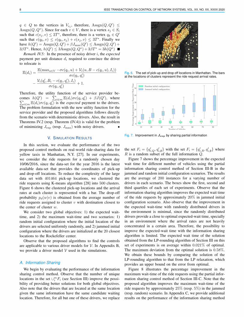
Fig. 6. The set of pick-up and drop off locations in Manhattan. The barsat the locations of clusters represent the ride request arrival rates.

10 20 30 40 50 60 70 80Number of Vehicles

0

10

20

30

40

50

Per

cent

age

Imp

rove

men

tin

Exp

ecte

dW

ait

Tim

e

Random initial configuration

Jammed initial configuration

Fig. 7. Improvement in Jexp by sharing partial information

the set Fi = {q′i,Q, q′i,∅} with the set Fi = {q′i,R, q′i,∅} whereR is a random subset of the full information Q.

Figure 7 shows the percentage improvement in the expectedwait time for different number of vehicles using the partialinformation sharing control method of Section III-B in thejammed and random initial configuration scenarios. The resultsare the average of 200 instances for a varying number ofdrivers in each scenario. The boxes show the first, second andthird quartiles of each set of experiments. Observe that theinformation sharing algorithm improves the expected wait timeof the ride requests by approximately 20% in jammed initialconfiguration scenario. Also observe that the improvement inthe expected wait-time with randomly distributed drivers inthe environment is minimal, since the randomly distributeddrivers provide a close to optimal expected-wait time, speciallyin an environment where the arrival rates are not heavilyconcentrated in a certain area. Therefore, the possibility toimprove the expected-wait time with the information sharingalgorithm is limited. The expected wait time of the solutionobtained from the LP-rounding algorithm of Section III on thisset of experiments is on average within 0.021% of optimal.The maximum deviation from the optimal solution is 0.58%.We obtain these bounds by comparing the solution of theLP-rounding algorithm to that from the LP relaxation, whichprovides an upper bound on the error from optimal.

Figure 8 illustrates the percentage improvement in themaximum wait-time of the ride requests using the partial infor-mation sharing control method of Section III-C. Note that theproposed algorithm improves the maximum wait-time of theride requests by approximately 25% (resp. 5%) in the jammed(resp. random) scenario. In Appendix C, we provide additionalresults on the performance of the information sharing method



0

10

20

30

40

50

60

70

Per

cent

age

Imp

rove

men

tin

Max

imu

mW

ait

Tim

eRandom initial configuration

Jammed initial configuration

Fig. 8. Improvement in Jmax by sharing partial information

in a system of 80 drivers responding to 300 ride requests.

B. Pay to Control

In this section, we evaluate the performance of the pay-to-control method for the jammed and random scenarios.Figure 9(a) illustrates the improvement in the expected andthe maximum wait-time for the two scenarios with β = 100.Note that the proposed algorithm improves the expected wait-time by approximately 75% (resp. 35%) for the jammed(resp.random) scenario. Also observe that the proposed algo-rithm improves the maximum wait-time by approximately 70%(resp. 50%) in the jammed (resp. random) scenario.

Figure 9(b) shows the payment per driver for the twoobjectives and the two scenarios. Observe that the expectedprofit of the drivers in the jammed scenario is smaller than theexpected profit of the drivers in the random scenario, therefore,the amount paid to convince the drivers to relocate to desiredwaiting locations in the jammed scenario is significantlysmaller compared to the amount paid in the random scenario.

Figure 10 shows the expected response time of a set of80 drivers responding to 300 requests arriving over time withthe jammed initial configuration. The results are an averageof 100 experiments with 300 randomly generated requests foreach experiment. The lines represent the average and shadedareas represent the first and third quartiles. The pay-to-controlis applied to the system if the expected-wait time is greaterthan 3 minutes. Observe that the proposed algorithm maintainsthe low expected wait-time in the course of servicing 300 riderequests. The average pay to maintain the low expected wait-time is 1.95$ per ride request. Figure 11 shows the sameexperiment with the objective of minimizing the maximumwait-time. The pay-to-control is applied to the system if themaximum wait time is greater than 7 minutes. The averagepay to maintain the low expected wait-time is 1.58$ per ride.

In summary, the experiments on the real-world ride-sharingdata show that the proposed algorithms significantly improvethe expected or the maximum wait-time when the driversare concentrated in a region. In particular, given a jammedconfiguration of the drivers, the proposed algorithms improvethe service quality significantly with a small number of controlinputs and maintain the same quality over-time. The improve-ments are more evident for the social objective of minimizingthe maximum wait-time, since the natural dynamics of thesystem tend to steer drivers away from the low-demand areas.


30

40

50

60

70

80

90

Per

cent

age

Imp

rove

men

tin

Ser

vice

Qu

alit

y

Jexp - Jammed configuration

Jexp - Random configuration

Jmax - Jammed configuration

Jmax - Random configuration

(a) The percentage improvement in the service quality


1.0

0.2

0.5

2.0

3.0

Ave

rage

Pay

men

tp

erD

rive

r($

)

Jexp - Jammed configuration

Jexp - Random configuration

Jmax - Jammed configuration

Jmax - Random configuration

(b) The amount paid to drivers

Fig. 9. Improvement in the global objectives and the amount paid todrivers using pay-to-control method. The blue (resp. green) representsthe results for the objective Jexp (resp. Jmax). The solid bars (resp.hatched bars) represent the jammed (resp. random) initial configuration.

0 50 100 150 200 250 300Number of Ride Requests

0

2

4

6

8

10

12

14

Exp

ecte

dW

ait

Tim

e(m

in)

No Control

Pay-To-Control

Paid Amount

0.0

2.5

5.0

7.5

10.0

12.5

15.0

17.5

20.0

Am

ount

Pai

dto

Dri

vers

($)

Fig. 10. The expected wait time and the paid amount to a system of 80drivers executing 300 ride requests under the pay-to-control method


10.0

6

789

20

30

40

50

60

Max

imu

mW

ait

Tim

e(m

in)

No Control

Pay-To-Control

Paid Amount

0.0

2.5

5.0

7.5

10.0

12.5

15.0

17.5

20.0

Am

ount

Pai

dto

Dri

vers

($)

Fig. 11. The maximum wait time and the paid amount to a system of80 drivers executing 300 ride requests under the pay-to-control method


Therefore, the control from the proposed algorithm is requiredto maintain equal service quality across different regions.

VI. DISCUSSION

The proposed control methods do not assume any specificform for the driver model, however, they assume that the drivermodel is known. Later, we extended the algorithms to captureuncertainty in the behavior of the drivers. For the informationsharing method, we substituted the cost of servicing a riderequest by a driver with the expected cost of servicing theride request, and for the pay-to-control method we replacedthe compensation with the expected payment to convince thedrivers to relocate. A disadvantage to this approach is that ifthe uncertainty in the driver model is high, then the expectedcost of servicing a ride requests and the expected payment canbecome prohibitively high, and the proposed algorithms willopt to not input any control into the system.

Another short-coming of the proposed methods is the scal-ability with the number of drivers in the systems due to thecombinatorial nature of our proposed approach. The alternativeapproach to these problems is to use a flow-model. However,this approach suffers scalability issues with the number ofregions (stations) in the system. In the flow-model approaches,the environment is usually divided to a small number ofregions. A promising direction is to utilize the proposedmethods in junction with a flow-model approach, where thesolution to the flow-model approach provides the number ofdrivers in each region, and our proposed methods optimallydistribute the drivers within the regions.

VII. CONCLUSION

This paper considered the problem of controlling self-interested drivers in ride-sharing applications. Two indirectcontrol methods were proposed and for each, a near-optimalalgorithm was presented. The extensive results show signifi-cant improvement in the expected wait-time and the maximumwait-time on real-world ride-sharing data. In addition, wehope to extend the results to capture vehicles with differentcapacities and to different ride-sharing applications.

REFERENCES

[1] L. Rayle, S. Shaheen, N. Chan, D. Dai, and R. Cervero, “App-based,on-demand ride services: Comparing taxi and ridesourcing trips anduser characteristics in san francisco university of california transportationcenter (uctc),” University of California, Berkeley, 2014.

[2] N. Diakopoulos. How Uber surge pricing really works. [Online].Available: https://www.washingtonpost.com/news/wonk/wp/2015/04/17/how-uber-surge-pricing-really-works/

[3] A. Rosenblat and L. Stark, “Algorithmic labor and information asym-metries: A case study of Ubers drivers,” International Journal OfCommunication, 2016.

[4] A. Sadeghi and S. L. Smith, “On re-balancing self-interested agentsin ride-sourcing transportation networks,” in IEEE 58th Conference onDecision and Control, 2019, pp. 5119–5125.

[5] W. Zhang, S. Guhathakurta, J. Fang, and G. Zhang, “The performanceand benefits of a shared autonomous vehicles based dynamic ridesharingsystem: An agent-based simulation approach,” in Transportation Re-search Board 94th Annual Meeting, no. 15-2919, 2015.

[6] M. Hyland and H. S. Mahmassani, “Dynamic autonomous vehicle fleetoperations: Optimization-based strategies to assign AVs to immediatetraveler demand requests,” Transportation Research Part C: EmergingTechnologies, vol. 92, pp. 278–297, 2018.

[7] M. Chang, D. S. Hochbaum, Q. Spaen, and M. Velednitsky, “DIS-PATCH: an optimal algorithm for online perfect bipartite matching withi.i.d. arrivals,” CoRR, vol. abs/1805.02014, 2018.

[8] M. Maciejewski, J. Bischoff, and K. Nagel, “An assignment-based ap-proach to efficient real-time city-scale taxi dispatching,” IEEE IntelligentSystems, vol. 31, no. 1, pp. 68–77, 2016.

[9] Uber. Driving with Uber, wait less, earn more. [Online]. Available:www.uber.com/ca/en/price-estimate/

[10] M. Pavone, S. L. Smith, E. Frazzoli, and D. Rus, “Robotic load balancingfor mobility-on-demand systems,” The International Journal of RoboticsResearch, vol. 31, no. 7, pp. 839–854, 2012.

[11] M. Tsao, R. Iglesias, and M. Pavone, “Stochastic model predic-tive control for autonomous mobility on demand,” arXiv preprintarXiv:1804.11074, 2018.

[12] G. C. Calafiore, C. Novara, F. Portigliotti, and A. Rizzo, “A flowoptimization approach for the rebalancing of mobility on demandsystems,” in IEEE International Conference on Decision and Control,2017, pp. 5684–5689.

[13] M. Salazar, F. Rossi, M. Schiffer, C. H. Onder, and M. Pavone, “On theinteraction between autonomous mobility-on-demand and public trans-portation systems,” in 2018 21st International Conference on IntelligentTransportation Systems (ITSC), 2018, pp. 2262–2269.

[14] G. P. Cachon, K. M. Daniels, and R. Lobel, “The role of surge pricingon a service platform with self-scheduling capacity,” Manufacturing andService Operations Management, vol. 19, no. 3, pp. 368–384, 2017.

[15] Q. Wei, J. A. Rodriguez, R. Pedarsani, and S. Coogan, “Ride-sharingnetworks with mixed autonomy,” in American Control Conference, 2019,pp. 3303–3308.

[16] S. Banerjee, R. Johari, and C. Riquelme, “Pricing in ride-sharing plat-forms: A queueing-theoretic approach,” in Proceedings of the SixteenthACM Conference on Economics and Computation, 2015, pp. 639–639.

[17] D. B. Shmoys, “Approximation algorithms for facility location prob-lems,” in International Workshop on Approximation Algorithms forCombinatorial Optimization. Springer, 2000, pp. 27–32.

[18] V. Arya, N. Garg, R. Khandekar, A. Meyerson, K. Munagala, andV. Pandit, “Local search heuristics for k-median and facility locationproblems,” SIAM Journal on computing, vol. 33, no. 3, pp. 544–562,2004.

[19] E. D. Demaine, M. Hajiaghayi, H. Mahini, A. S. Sayedi-Roshkhar,S. Oveisgharan, and M. Zadimoghaddam, “Minimizing movement,”ACM Transactions on Algorithms (TALG), vol. 5, no. 3, p. 30, 2009.

[20] A. Sadeghi and S. L. Smith, “Re-deployment algorithms for multipleservice robots to optimize task response,” in IEEE International Con-ference on Robotics and Automation, 2018, pp. 2356–2363.

[21] S. Bandyapadhyay, A. Banik, S. Das, and H. Sarkar, “Voronoi game ongraphs,” Theoretical Computer Science, vol. 562, pp. 270–282, 2015.

[22] R. Salhab, J. Le Ny, and R. P. Malhame, “A dynamic ride-sourcinggame with many drivers,” in 55th Annual Allerton Conference onCommunication, Control, and Computing, 2017, pp. 770–775.

[23] T. Basar and G. J. Olsder, Dynamic noncooperative game theory. Siam,1999, vol. 23.

[24] S. Ahmadian, Z. Friggstad, and C. Swamy, “Local-search based approx-imation algorithms for mobile facility location problems,” in Proceed-ings of the twenty-fourth annual ACM-SIAM symposium on Discretealgorithms. SIAM, 2013, pp. 1607–1621.

[25] V. V. Vazirani, Approximation algorithms. Springer Science & BusinessMedia, 2013.

[26] R. Jonker and T. Volgenant, “Improving the hungarian assignmentalgorithm,” Operations Research Letters, vol. 5, no. 4, pp. 171–175,1986.

[27] (2016) TLC yellow taxi trip data set. [Online]. Available: https://www1.nyc.gov/site/tlc/about/tlc-trip-record-data.page

[28] F. Pedregosa, G. Varoquaux, A. Gramfort, V. Michel, B. Thirion,O. Grisel, M. Blondel, P. Prettenhofer, R. Weiss, V. Dubourg, J. Vander-plas, A. Passos, D. Cournapeau, M. Brucher, M. Perrot, and E. Duch-esnay, “Scikit-learn: Machine learning in Python,” Journal of MachineLearning Research, vol. 12, pp. 2825–2830, 2011.

[29] R. Schuler, “An algorithm for the satisfiability problem of formulas inconjunctive normal form,” Journal of Algorithms, vol. 54, no. 1, pp.40–44, 2005.

[30] L. Breiman, “Random forests,” Machine learning, vol. 45, no. 1, pp.5–32, 2001.

[31] The Canadian Automobile Association. Driving costs. [Online].Available: www.carcosts.caa.ca/


APPENDIX

A. Proof of Results

Proof: [Proof of Theorem 3.4] We prove the NP-hardnessof Problem III.3 for minimizing the expected wait-time Jexpwith a reduction from CNF-SAT [29] as follows:

Consider an instance of CNF-SAT with m Boolean variablesand n clauses. Now we construct an instance of Problem III.3.

(i) For each variable xi of the CNF-SAT instance, we createa set Fi = {vTi , vFi }, where vTi will correspond tosetting the xi to true and vFi will correspond to settingit to false.

(ii) We let V contain n vertices, one representing eachclause in the SAT formula.

(iii) Let E contain an edge for each v ∈ ∪mi=1Fi and w ∈ V .(iv) For each e = (v, w) ∈ E, we set its cost to 1 if the literal

v appears in the clause w, and 2 if the literal does not.Note that the costs are metric.

(v) Let pa(u) = 1/n for each u ∈ V .

Now, we solve the instance of Problem III.3 with theobjective of minimizing the expected wait-time Jexp. If itreturns a subset of ∪mi=1Fi with cost exactly 1, then for vertexc ∈ V , there is a vertex v in ∪mi=1Fi with edge cost of 1 to c.Vertex c corresponds to a clause and vertex v corresponds to aliteral in c. This implies that the literal chosen from each subsetin the partition of ∪mi=1Fi gives a satisfying truth assignmentfor the SAT instance. If the subset returned has a cost greaterthan 1, then there exists a clause w ∈ V for which everychosen literal has an edge cost of 2. Thus, this clause is notsatisfied and no satisfying instance exists.

Proof: [Proof of Theorem 3.5] The proof of hardness forProblem III.3 with the objective Jmax follows the same stepsas the proof of Theorem III.4 with exception of step (v) wherepa(u) = 1 for each u ∈ V .

Proof: [Proof of Lemma 3.6] By contradiction assumethere is a conflict in Subroutine II. Therefore, at some stepof the execution, there is a vertex v such that |Nk(v)| = 0.Prior to this step, |Nk−1(v)| = 1, and there should have beenanother vertex w with |Nk−1(w)| = 1, otherwise the algorithmwould have added the vertex in Nk−1(v) to the solution.Observe that the event of |Nk−1(w)| = 1 and |Nk−1(v)| = 1shows that at the start of Subroutine II, Ni(w) ∩ Ni(v) 6= ∅for an i < k. Let q1 ∈ Nk−1(v), q2 ∈ Nk−1(w) andz ∈ Ni(w) ∩ Ni(v). Without loss of generality, assume thatqi, qj and ql correspond to the expected waiting location of thedrivers i, j and l where no information is provided to them.Then the cost of servicing v with giving no information todriver j is c(v, qj) ≤ c(w, qj) + c(w, v) and also note thatc(w, v) ≤ c(w, ql) + c(v, ql) by the triangle inequality.

Therefore, the time to service v by driver j with noinformation is c(v, qj) ≤ c(w, qj) + c(w, v) ≤ c(w, qj) +c(w, ql) + c(v, ql) ≤ 3T . Thus, v would have been marked asserviced prior to conflict.

Proof: [Proof of Corollary 3.8] We omit the detailed proofdue to space constraints, however, the proof directly followsfrom the proof of Lemma III.6 and Theorem III.7 with only

the following modification in the proof of Lemma III.6:

c(v, qj) =∑z∈V

pjw(z, ∅)c(z, v) ≤∑z∈V

pjw(l, ∅)c(l, w) + c(w, v)

≤ c(w, qj) +∑z∈V

plw(l, ∅)c(z, v) +∑l∈V

plw(z, ∅)c(z, w)

≤ c(w, qj) + c(w, ql) + c(v, ql) ≤ 3T.

Proof: [Proof of Lemma 4.3] Suppose, T ∗ < c(ei), thenfor vertex v ∈ V there is a vertex in q ∈ Q∗, denoted by`Q∗(v), with c(q, v) ≤ T ∗. Observe that for any sj , sk ∈Si, we have `Q∗(sj) 6= `Q∗(sk), otherwise, there is an edgebetween sj , sk in graph H2

i . This is a contradiction since Si isa maximal independent set. Therefore, for each vertex in Si,there is a unique vertex in Q∗. This is a contradiction, since|Q∗| = m.

B. Drivers’ model

A driver model is a function for evaluating the expectedprofit of different locations at each time instance. The drivermodel of the drivers in Section V takes into account theenvironmental parameters such as arrival rates and drop-offprobabilities and the information shared with the driver. Letpi(v, u) be the probability that a ride-request at v is assignedto driver i positioned at u with information Ii. Then, we findthe perception of expected profit of a driver as follows:

Vi(u,Bi, Ii) =∑v,w∈V

pd(w|v)[pi(v, u)

(max{0, σ′c(w, v)

− σc(u, v) + Vi(w,Bi − c(u, v)− c(v, w), Ii)})], (8)

Note that the calculation of the expected profit of driversfor each time step is computationally expensive, thus wetrained a Random Forest Regressor [30] implemented by [28]to approximate the values of V for each number of vehiclesin the system with training data over 10000 instances withwork-day Bi of 15 average length rides, fare σ′ = $0.81 perkilometer [9] and driving cost σ = $0.15 per kilometer [31].

We refer the reader to [4] for a detailed description of themodel and the proposed method for computing pi(v, u).


4

6

8

10

12

14

Exp

ecte

dW

ait-

Tim

e(m

in)

Information Sharing Control

No Control

Fig. 12. The expected wait-time of ride requests in a system of 80drivers executing 300 ride requests arriving over time under the partialinformation control method.



20

25

30

35

40

45

50

55M

axim

um

Wai

tT

ime

(min

)Information Sharing Control

No Control

Fig. 13. The maximum wait-time of ride requests in a system of 80drivers executing 300 ride requests arriving over time under the partialinformation control method.

TABLE IIINFORMATION SHARING FOR NOISY DRIVERS

Initial Configuration Jexp Jmax

Avg. Std. Dev. Avg. Std. Dev.

Random 2.4 0.3 21.8 10.1Jammed 43.2 4.0 54.7 6.1

C. Information Sharing in a Horizon

Figure 12 shows the expected response time of a set of80 drivers responding to 300 requests arriving over time withthe jammed initial configuration. The figure summarizes 100experiments with 300 randomly generated requests for eachexperiment. The lines represent the average and shaded areasrepresent the first and third quartiles. In the transient, theinformation sharing algorithm improves the expected responsetime rapidly. However, in the steady-state the performance isvery similar to the no control case. Thus, the informationsharing method serves to more quickly disperse the driversfrom the initial jammed configuration. The information sharingalgorithm is applied whenever the expected wait time is largerthan 6 minutes. Figure 13 shows the similar experiment withthe objective of minimizing the maximum wait-time. Observethat the proposed algorithm improves the maximum wait-timein the initial jammed configuration and maintains the qualityservice over the course of responding to 300 requests. Tolimit the number of information sharing control inputs to thesystem, we only use the information sharing method whenthe maximum wait time in the current driver configuration islarger than 30 minutes.

D. Information Sharing for Noisy Drivers

In this section, we evaluate the performance of the proposedinformation control method in the presence of noisy drivers.We model the uncertainty in the behaviour of the driver (seeEquation (5)) with a zero mean uniform noise Zu at eachvertex where the maximum deviation from Vi(u,Bi, Ii) is20%. Table II shows the improvement in the expected wait-time Jexp and the maximum wait-time Jmax for the twoscenarios. The results are the average of 200 trials for eachglobal objective and each initial configuration of the drivers.Observe that the proposed algorithms for the information shar-

ing problem with noisy drivers provide similar performanceto the ones with deterministic drivers under random initialconfiguration. However, the performance of the algorithmsimprove with uncertainty in the behavior of the drivers underjammed initial configuration. Observe that in the jammedinitial configuration with deterministic drivers, the driversinitialized at the same location have similar optimal waitinglocations if full-information is provided to them. Therefore,the algorithms provide the information to only one of thedrivers positioned at each vertex. However, in the presence ofnoisy drivers, if full information is provided to multiple driversposition at the same location, the drivers relocate to differentwaiting locations. Therefore, the algorithms opt to provideinformation to more drivers resulting in a better distributionof drivers in the environment.

re-balancing self-interested drivers in ride-sharing

Documents