rd ideal function v2
TRANSCRIPT
Performance characterization
Don Clausing
© Don Clausing 1998
16.881 Fig. 1

Failure modes
• Noises lead to failure modes (FM) • One set of noise values leads to FM1
• Opposite set of noise values leads to FM2
• Simple problem solving chases the problem from FM1 to FM2 and back again, but does not avoid both FMs with the same set of design values – endless cycles of build/test/fix (B/T/F)
© Don Clausing 1998
16.881 Fig. 2
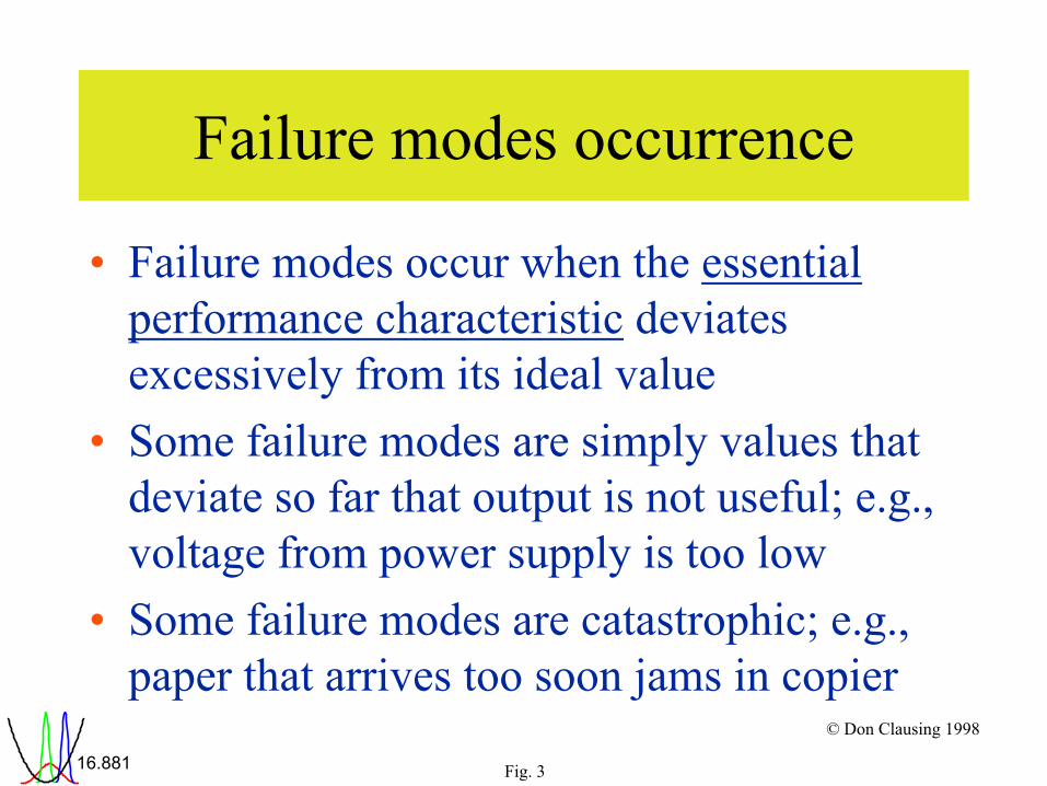
Failure modes occurrence
• Failure modes occur when the essential performance characteristic deviates excessively from its ideal value
• Some failure modes are simply values that deviate so far that output is not useful; e.g., voltage from power supply is too low
• Some failure modes are catastrophic; e.g., paper that arrives too soon jams in copier
© Don Clausing 1998
16.881 Fig. 3

Performance characteristic
• What is good performance characteristic to use when reducing the occurrence of failure modes?
• Don’t merely count occurrence of failure modes
• Can’t distinguish between following two cases
© Don Clausing 1998
16.881 Fig. 4

Case 1 – easy to fix
Occurrence offailure mode
FM1 FM2© Don Clausing 1998
16.881 Fig. 5
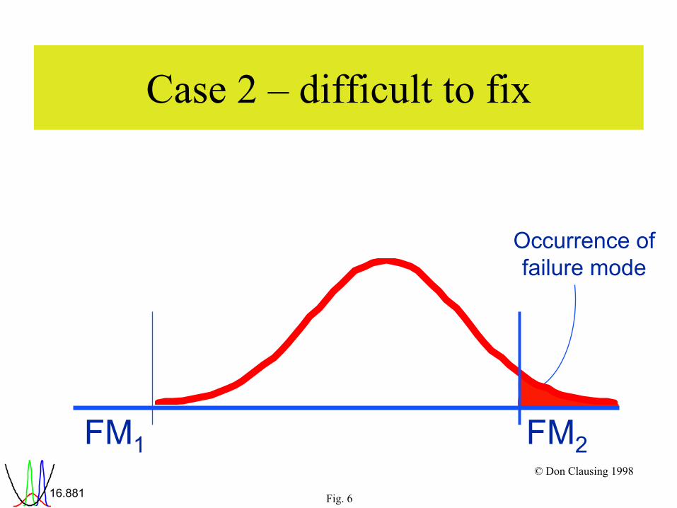
Case 2 – difficult to fix
Occurrence offailure mode
FM1 FM2© Don Clausing 1998
16.881 Fig. 6

Case 1 and Case 2
• Both cases have same failure rate • But situations are very different • Counting failure rate is very weak approach
to the reduction of failure rate • Concentrate on ideal function –
What is the system supposed to do? • Then make system do it all of the time
© Don Clausing 1998
16.881 Fig. 7

The engineered system
Noise
Signal System Response
Controlfactors
© Don Clausing 1998
16.881 Fig. 8

Ideal function
Ideal function
(response)
RES
PON
SE
SIGNAL, M © Don Clausing 1998
16.881 Fig. 9
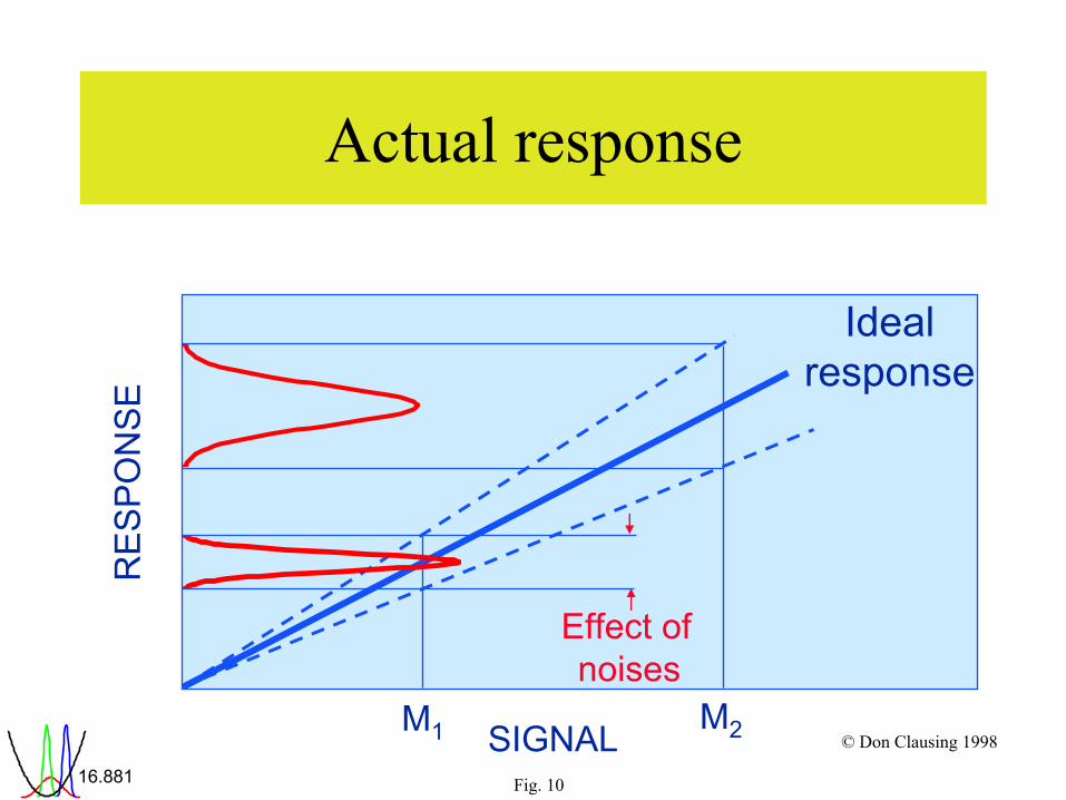
Actual response
Ideal response
Effect of noises
RES
PON
SE
M1 SIGNAL M2 © Don Clausing 1998
16.881 Fig. 10

Keep performance close to ideal
• Identify ideal performance (function, response)
• Then make actual performance stay as close as possible to ideal
• Linear response is called “dynamic” – desired value for response depends on input value of signal
© Don Clausing 1998
16.881 Fig. 11

Examples of dynamic response
• Car turning radius • Car stopping distance • Copy quality • Casting • Electrical resistance
What are the signals?
© Don Clausing 1998
16.881 Fig. 12

Case study – hitch
• Used to connect implements to tractor • Transmits power from tractor to implement • We can all see its function • But what is a good engineering statement of
its function?
© Don Clausing 1998
16.881 Fig. 13
Functions of hitch
• Provide mechanical interface with implement • Provide proper vehicle performance • Meet ISO dimensional requirements • Protect people from moving parts
© Don Clausing 1998
16.881 Fig. 14
More detail on first function • Provide adequate performance in working range
– Proper attitude through working range – Provide adequate depth – Provide adequate lift capacity at breakout – Provide Draft Control
• Provide adequate performance in transport mode – Provide adequate height – Provide proper kick angle – Provide adequate lift capacity at transport
• Provide easy hookup and disconnect • Provide easy linkage adjustments
© Don Clausing 1998
16.881 Fig. 15
Yes, but what is ideal function?
• Meet ISO dimensional requirements • Protect people from moving parts are important
generic requirements, but are not elements of the ideal function.
© Don Clausing 1998
16.881 Fig. 16
Functions of hitch
• Provide mechanical interface with implement • Provide proper vehicle performance are
related to ideal function. Candidate for ideal function: Transmit load
© Don Clausing 1998
16.881 Fig. 17

Forces on system
H I T C H
IMPLEMENT TRACTOR
FT
FFFD
WH
FRFS
© Don Clausing 1998
16.881 Fig. 18

Noises in the field
HARD ROWS
• Change in earth impedance causes forces to change • Which changes do we wish to minimize?
© Don Clausing 1998
16.881 Fig. 19

Keep what constant?
• Constant force? • Constant depth of engagement into the soil? • Constant power?
© Don Clausing 1998
16.881 Fig. 20

Candidate ideal function
Actualdepth
Ideal function
(response)
SIGNAL, depth set by farmer
© Don Clausing 1998
16.881 Fig. 21
Determination of ideal function
• Identify the performance variations that we would like to go to zero
• The performance that remains when the undesirable variations are zero is the ideal performance
• In the hitch case further analysis, tests, and discussions with customers are needed to identify (verify) ideal function
© Don Clausing 1998
16.881 Fig. 22

Ideal function
• Want Ideal Response to Signal – usually straight-line function
• Definition is often not trivial • In the absence of explicit definition the
objective of improvement activities is unclear; success unlikely
© Don Clausing 1998
16.881 Fig. 23

Signal/noise ratio
• Measure of deviation from ideal performance
• Based on ratio of deviation from straight line divided by slope of straight line
• Many different types – depends on type of performance characteristic
• Larger values of SN ratio represent more robust performance
© Don Clausing 1998
16.881 Fig. 24

Summary
• Knowing ideal function is crucial for success – we have to know where we are trying to get to, or it is unlikely that we will get there in a reasonable time
• Requires detailed engineering analysis of conditions for customer satisfaction
© Don Clausing 1998
16.881 Fig. 25

End