rate-controlled constrained-equilibrium (rcce) modelling ...1599/... · rate-controlled...
TRANSCRIPT

Rate-Controlled Constrained-Equilibrium (RCCE) Modelling of C1-Hydrocarbon Fuels
A Dissertation Presented
By
Mohammad Janbozorgi
to
The Department of Mechanical and Industrial Engineering
in partial fulfilment of the requirements for the degree of
Doctor of Philosophy
in the field of
Mechanical Engineering
Northeastern University Boston, Massachusetts
August 2011
2
Dedicated to the memory of
Prof. James C. Keck
who introduced me to the wonderful world of
Constrained Equilibrium

3
Contents
Acknowledgments .......................................................................................................... 5 Abstract ........................................................................................................................... 7
Introduction ................................................................................................................. 8 Chapter 1 ........................................................................................................................... 12 Combustion Modelling of Mono-Carbon Fuels Using the Rate-Controlled Constrained-
Equilibrium Method .......................................................................................................... 13 2.1 Introduction ................................................................................................... 14 2.2 Rate-Controlled Constrained-Equilibrium (RCCE) Method ........................ 16
1.2.1 Rate-equations for the constraints ......................................................... 18 1.2.2 Rate equations for the constraint potentials .......................................... 19
2.3 Selection of constraints ................................................................................. 21 2.4 Determination of initial conditions ............................................................... 24 2.5 RCCE calculations for C1 hydrocarbon oxidation ........................................ 26
1.5.1 Methane (CH4) oxidation ..................................................................... 27 1.5.2 CH4 Results for Full 133 reaction set .................................................. 29 1.5.3 Methanol (CH3OH) oxidation ............................................................... 32 1.5.4 Reduced CH3OH reaction mechanism .................................................. 32 1.5.5 Formaldehyde (CH2O) oxidation .......................................................... 32
2.6 Summary and conclusions ............................................................................ 33 2.7 Acknowledgment .......................................................................................... 34 2.8 References ..................................................................................................... 34
Chapter 2 ........................................................................................................................... 54 Combustion Modelling of Methane-Air Mixtures Using the Rate-Controlled Constrained-Equilibrium Method .......................................................................................................... 54
2.1 Introduction ................................................................................................... 55 2.2 Rate-Controlled Constrained-Equilibrium .................................................... 57
Table 2.1: C1/C2 constraints .............................................................................................. 57 2.3 Results and discussions ................................................................................. 58
2.3.1 C1/C2 oxidation ..................................................................................... 58 2.3.2 Comparison with shock tube data ......................................................... 59
2.4 Summary and conclusions ............................................................................ 59 2.5 References ..................................................................................................... 63
Chapter 3 ........................................................................................................................... 65 Rate-Controlled Constrained-Equilibrium Theory Applied to Expansion of Combustion
Products in the Power Stroke of an Internal Combustion Engine .................................... 65 3.1 Introduction ................................................................................................... 66 3.2 Physical model .............................................................................................. 67 3.3 Governing equations in RCCE form ............................................................. 68 3.4 Constraints .................................................................................................... 71 3.5 Results and discussion .................................................................................. 72 3.6 Concluding remarks ...................................................................................... 76 3.7 Nomenclature ................................................................................................ 77 5.3 References ..................................................................................................... 78

4
Chapter 4 ........................................................................................................................... 80 Rate-Controlled Constrained-Equilibrium Theory Applied to Expansion of Combustion
Products in the Power Stroke of an Internal Combustion Engine ........................................ 4.1 Introduction ................................................................................................... 81 4.2 Model ............................................................................................................ 82 4.3 RCCE form of the equations ......................................................................... 83 4.4 Area profile ................................................................................................... 83 4.5 Constraints .................................................................................................... 84 4.6 Results and discussions ................................................................................. 85 4.7 RDX reacting system .................................................................................... 90 4.8 References ..................................................................................................... 91
Chapter 5 ........................................................................................................................... 92 Conclusions and Future Works ......................................................................................... 93
5.1 Conclusions ................................................................................................... 94 5.2 Future Works ................................................................................................ 96

5
Acknowledgments
I have been fortunate enough to benefit from the following people during the course of
my PhD, whom I wish to thank:
Prof. Hameed Metghalchi - Principal Advisor: Thank you for being such a great friend
and a wonderful mentor. I never forget how happily I always walked out of your office
regardless of how grumpy I walked in.
Prof. James C. Keck of MIT – Co-advisor: I learned virtually everything I learned in my
PhD from you, directly or indirectly through the challenge and the incredible insight that
you brought into the group.
Prof. Yannis Levendin and Prof. Reza Sheikhi: Thank you for serving on my
committee and for all the scientific talks that we have had.
Prof. John Cipolla: I took all the essential courses I needed for my research with you.
My observation from your classes was that you are a gifted teacher, who is at the same
time a remarkable researcher. Thank you for all the deep and insightful discussions we
always had.
The staff of the Mechanical and Industrial Engineering Department: Noah Japhet, Joyce
Crain, LeBaron Briggs and Richard Weston, Thank you for always being there for
graduate students and for being so supportive.
My great friends: Dr. Farzan Parsinejad – I always enjoyed talking to you; Dr. Kian
Eisazadeh Far – You always kept me engaged in thinking about thoughtful questions and
very insightful discussions; Dr. Donald Goldthwaite - thank you for very interesting
discussions we always had on RCCE and different aspects of it. It has been a pleasure to
work along with you; Dr. Yue Gao, thank you very much for getting me started on
RCCE. Also, special thanks to all my great friends, including, but most definitely not
limited to, Ghassan Nicolas, Ali Moghaddas, Casy Benett, Mimmo Illia, Jason Targoff,
Adrienne Jalbert, Mehdi Abedi, Ramin Zareian, Reza Khatami, Mehdi Safari, Fatemeh
Hadi and many others.

6
All the practitioners at C.W. Taekwondo at Boston and RedlinefightSports at
Cambridge: The time I spent training with you was without a doubt some of the most
precious time I have had in my entire life. I could not imagine any way of releasing the
anxiety more efficient than training with you and enjoying the great friendships that
developed along the way.
Last but certainly not least, my family for always providing me with their never ending
love and support.
Thank you all very much!
7
Abstract This dissertation is focused on an important problem faced in chemical kinetic
modelling, that is, model order reduction. The method of Rate-Controlled Constrained-
Equilibrium (RCCE) firmly based on the Second Law of Thermodynamics, has been
further developed and used for this purpose. The main challenge in RCCE lies in
selection of the kinetic constraints. Two classes of problems were looked at: 1) far-from-
equilibrium problem of ignition and 2) relaxations away from equilibrium due to
interactions with the environment.
Regarding the first class, a unified RCCE model for combustion of C1-
hydrocarbon fuels (CH4, CH3OH and CH2O) and their corresponding reduced models
were developed. The model is composed of a set of structural constraints controlling the
chemical conversion from fuel into combustion products.
For the second class it was shown that a subset of the constraints identified in the
first class is able to equally well predict the main features of expansion of combustion
products within the power stroke of an internal combustion engine as well as supersonic
expansion through a rocket nozzle and also expansion through a heat exchanger as a
model for sudden cooling in gas turbine.
A method based on the degree of disequilibrium of chemical reactions was also
suggested for selection of kinetic constraints. This approach has potentials to reduce the
level of chemical knowledge required for selection of kinetic constraints and it was
shown how the application of this method reproduces the generalized constraints used in
the second class of problems without any chemical intuition.
8
Introduction The development of models for describing the time evolution of chemically reacting
systems is a fundamental objective of chemical kinetics. The conventional approach to
this problem involves first specifying the state and species variables to be included in the
model, compiling a “full set” of rate-equations for these variables, and integrating this set
of equations to obtain the time-dependent behaviour of the system. Such models are
frequently referred to as “detailed kinetic models” (DKM). The problem is that the
detailed kinetics of C/H/O/N molecules can easily involve hundreds of chemical species
and isomers, and thousands of possible reactions even for system containing only C1
molecules. Clearly, the computational effort required to treat such systems is extremely
large. The difficulties are compounded when considering reacting turbulent flows, where
the complexity of turbulence is added to that of the chemistry.
As a result a great deal of effort has been devoted to developing methods for
simplifying the chemical kinetics of complex systems. Among the most prominent are:
Quasi Steady State Approximation (QSSA) [1], Partial Equilibrium Approximation [2],
Intrinsic Low Dimensional Manifolds (ILDM) [3], Computational Singular Perturbation
(CSP) [4], Adaptive Chemistry [5], Directed Relation Graph (DRG) [6] and The ICE-PIC
method [7].
A common problem shared by all the above methods is that they start with DKMs
containing a large number of reactions for which only the orders of magnitude of the
reaction-rates are known. Thus, unless the simplified model effectively eliminates these
uncertain reactions, the resulting model will be equally uncertain. The question is: If the
uncertain reactions are to be eliminated, does it make any sense to include them in the
first place?
An alternative approach, originally proposed by Keck and Gillespie [8] and later
developed and applied by Keck and co-workers [9-11], and others [12-15] is the Rate-
Controlled Constrained-Equilibrium (RCCE) method. This method is based on the
maximum-entropy principle of thermodynamics and involves the fundamental
assumption that slow reactions in a complex reacting system impose constraints on its
composition which control the rate at which it relaxes to chemical equilibrium, while the
fast reactions equilibrate the system subject to the constraints imposed by the slow

9
reactions. Consequently, the system relaxes to chemical equilibrium through a sequence
of constrained-equilibrium states at a rate controlled by the slowly changing constraints.
A major advantage of the RCCE method over the others mentioned above is that it
does not require a DKM as a starting point. Instead, one starts with a small number of
rate-controlled constraints on the state of a system, to which more can be systematically
added to improve the accuracy of the results. If the only constraints are those imposed by
slowly changing state variables, the RCCE method is equivalent to a local chemical
equilibrium calculation. If the constraints are the species, the RCCE model is similar to a
DKM having the same species with the important difference that RCCE calculations
always approach the correct final chemical equilibrium state whereas DKM calculations
do not. The reason for this is that the equilibrium state approached by a DKM contains
only the species included in the model whereas the equilibrium state approached by an
RCCE model includes all possible species that can be formed from the elements of which
it is composed.
As with all thermodynamic systems, the number of constraints necessary to describe
the state of the system within measurable accuracy can be very much smaller than the
number of species in the system. Therefore fewer equations are required to determine the
state of a system. A further advantage is that only the reaction-rates of slow reactions
which change the constraints are needed and these are the ones most likely to be known.
Reactions which do not change any constraint are not required. It should be emphasized
that the successful implementation of the RCCE method depends critically on the
constraints employed.
The structure of this thesis is as follows: in chapter 1 an RCCE model is developed
for C1 fuels of CH4, CH2O and CH3OH with detailed presentation of the working
equations under thermodynamic state variables (E,V) along with a method to initialize
the RCCE calculations. Three sets of reduced RCCE kinetic models for these fuels are
also presented, the union of which involves 20 elementary reactions and the same number
of species in the DKM. The model has the interesting feature of structurally constraining
the kinetic patterns of oxidations of these fuels down to CO2 and H2O. However, only the
C1 chemistry has been considered. This is so that in fuel rich mixtures or at higher
pressures where the recombination processes become important, the path to higher

10
hydrocarbons, more importantly C2 becomes more active. As a result, in chapter 2 the
interaction between C1 and C2 kinetics is considered and an extra set of three constraints
is identified. This set, when added to the previously discovered set, has an acceptable
predictive capability over the entire working range of the kinetic model. The importance
of C1 and C2 kinetics cannot be over-emphasized due to the fact that once the beta-
scission is activated, combustion of almost any hydrocarbon fuels, except for an
immediate fuel-molecule-dependent chemistry within the low temperature cycle, soon
becomes a matter of burning a mixture of C1/C2/C3 Components. This fact underlies the
observation that most straight chain hydrocarbon fuels have almost the same laminar
burning speeds.
In chapters 3 and 4 another class of problems, in which a highly dissociated
equilibrium mixture is thrown out of equilibrium due to interactions with the surrounding
environment, is looked at. The main question at this stage is whether or not a subset of
the kinetic constraints already identified for ignition of C1 and C2 is capable of predicting
the dynamic behaviour of the re-activated kinetic effects in these systems. It is shown, by
physical reasoning and rational analysis that the answer is yes. A rational for such a
question is that the equilibrium composition of almost all hydrocarbon fuels is almost
fuel independent and is mainly composed of the H/O and a number of C/H/O species and
is therefore, controlled by their corresponding kinetics. Chapter 3 specifically considers
expansion of combustion products within the power stroke of an internal combustion
engine and chapter 4 studies the kinetics of H/O relaxation within a supersonic nozzle.
The IC engine modelling assumes an adiabatic expansion, starting from equilibrium
products over a prescribed time-dependent volume. Also, in chapter 4 a new approach
based on the degree of disequilibrium (DOD) of chemical reactions is proposed for
selecting the kinetic constraints. It is shown there how the application of DOD
reconstructs, without any requirement of chemical kinetic knowledge, the generalized
constraints identified by physical reasoning in chapter 3. This method has been so far
applied only to starting-from-equilibrium problems, but has promising potentials to be
further extended to starting-from-a-non-equilibrium-state problems as well.
Chapter 5 draws conclusions and the future works.

11
Each chapter has been published in the literature as a separate paper and is therefore,
self contained. There are as a result, overlapping materials, equations and references
among different chapters.

12
Chapter 1

13
Combustion Modelling of Mono-Carbon Fuels Using the Rate-Controlled
Constrained-Equilibrium Method
Mohammad Janbozorgi a, Sergio Ugarte a, Hameed Metghalchi a, James. C. Keck b a Mechanical and Industrial Engineering Department, Northeastern University, Boston,
MA 02115, USA b Mechanical Engineering Department, Massachusetts Institute of Technology,
Cambridge, MA 02139, USA
Published in Combustion and Flame - Volume 156, Issue 10, October 2009, Pages 1871-
1885

14
Abstract
The Rate-Controlled Constrained-Equilibrium (RCCE) method for simplifying the
kinetics of complex reacting systems is reviewed. This method is based on the
maximum-entropy-principle of thermodynamics and involves the assumption that the
evolution of a system can be described using a relatively small set of slowly changing
constraints imposed by the external and internal dynamics of the system. As a result, the
number of equations required to determine the constrained state of a system can be very
much smaller than the number of species in the system. In addition, only reactions which
change constraints are required; all other reactions are in equilibrium. The accuracy of
the method depends on both the character and number of constraints employed and issues
involved in the selection and transformation of the constraints are discussed. A method
for determining the initial conditions for highly non-equilibrium systems is presented
The method is illustrated by applying it to the oxidation of methane (CH4), methanol
(CH3OH) and formaldehyde (CH2O) in a constant volume adiabatic chamber over a wide
range of initial temperatures and pressures. The RCCE calculations were carried out
using 8 to 12 constraints and 133 reactions. Good agreements with “detailed”
calculations using 29 species and 133 reactions were obtained. The number of reactions
in the RCCE calculations could be reduced to 20 for CH4, 16 for CH3OH and 12 for
CH2O without changing the results. “Detailed” calculations with less than 29 reactions
are indeterminate.
Keywords:, Rate-controlled Constrained-equilibrium, Maximum entropy principle,
Detailed modelling, Reduced kinetics, Methane, Methanol, Formaldehyde.
2.1 Introduction
The development of models for describing the time evolution of chemically reacting
systems is a fundamental objective of chemical kinetics. The conventional approach to
this problem involves first specifying the state and species variables to be included in the
model, compiling a “full set” of rate-equations for these variables, and integrating this set
15
of equations to obtain the time-dependent behaviour of the system. Such models are
frequently referred to as “ detailed kinetic model”s (DKM). The problem is that the
detailed kinetics of C/H/O/N molecules can easily involve hundreds of chemical species
and isomers, and thousands of possible reactions even for system containing only C1
molecules. Clearly, the computational effort required to treat such systems is extremely
large. The difficulties are compounded when considering reacting turbulent flows, where
the complexity of turbulence is added to that of the chemistry.
As a result a great deal of effort has been devoted to developing methods for
simplifying the chemical kinetics of complex systems. Among the most prominent are:
Quasi Steady State Approximation (QSSA) [1], Partial Equilibrium Approximation [2],
Intrinsic Low Dimensional Manifolds (ILDM) [3], Computational Singular Perturbation
(CSP) [4], Adaptive Chemistry [5], Directed Relation Graph (DRG) [6] and The ICE-PIC
method [7].
A common problem shared by all the above methods is that they start with DKMs
containing a large number of reactions for which only the orders of magnitude of the
reaction-rates are known. Thus, unless the simplified model effectively eliminates these
uncertain reactions, the resulting model will be equally uncertain. The question is: If the
uncertain reactions are to be eliminated, does it make any sense to include them in the
first place?
An alternative approach, originally proposed by Keck and Gillespie [8] and later
developed and applied by Keck and co-workers [9-11], and others [12-15] is the Rate-
Controlled Constrained-Equilibrium (RCCE) method. This method is based on the
maximum-entropy principle of thermodynamics and involves the fundamental
assumption that slow reactions in a complex reacting system impose constraints on its
composition which control the rate at which it relaxes to chemical equilibrium, while the
fast reactions equilibrate the system subject to the constraints imposed by the slow
reactions. Consequently, the system relaxes to chemical equilibrium through a sequence
of constrained-equilibrium states at a rate controlled by the slowly changing constraints.
A major advantage of the RCCE method over the others mentioned above is that it
does not require a DKM as a starting point. Instead, one starts with a small number of
rate-controlled constraints on the state of a system, to which more can be systematically
16
added to improve the accuracy of the results. If the only constraints are those imposed by
slowly changing state variables, the RCCE method is equivalent to a local chemical
equilibrium calculation. If the constraints are the species, the RCCE model is similar to a
DKM having the same species with the important difference that RCCE calculations
always approach the correct final chemical equilibrium state whereas DKM calculations
do not. The reason for this is that the equilibrium state approached by a DKM contains
only the species included in the model whereas the equilibrium state approached by an
RCCE model includes all possible species that can be formed from the elements of which
it is composed.
As with all thermodynamic systems, the number of constraints necessary to describe
the state of the system within measurable accuracy can be very much smaller than the
number of species in the system. Therefore fewer equations are required to determine the
state of a system. A further advantage is that only the reaction-rates of slow reactions
which change the constraints are needed and these are the ones most likely to be known.
Reactions which do not change any constraint are not required. It should be emphasized
that the successful implementation of the RCCE method depends critically on the
constraints employed.
The primary objectives of this paper are to (1) review the working equations required
to implement the RCCE method for chemically reacting systems, (2) discuss the issues
involved in the selection and transformation of the constraints, and (3) present a method
for determining the initial conditions for highly non-equilibrium systems for which
concentrations of some species are zero. To illustrate the method, RCCE calculations of
the oxidation of C1 hydrocarbon in a constant volume adiabatic chamber have been made
and compared with the results of a DKM.
2.2 Rate-Controlled Constrained-Equilibrium (RCCE) Method
A detailed description of the Rate-Controlled Constrained-Equilibrium (RCCE)
method is given in reference [16]. A concise summary of the working equations for
chemically reacting gas mixtures is given below.

17
It is assumed that energy exchange reactions are sufficiently fast to equilibrate the
translational, rotational, vibrational, and electronic degrees of the system subject to
constraints on the volume, V, and the total energy ,E, of the system. Under these
conditions, the energy can be written
NTEE T )(= (1.1)
where )(TET is the transpose of the species molar energy vector and T is the
temperature. It is further assumed that, consistent with the perfect gas model, the species
constraints, C, can be expressed as a linear combination of the species mole numbers, N,
in the form
NAC = (1.2)
where, A is the spc nn × constraint matrix, nc is the number of constraints ,spn is the
number of species and C and N are column vectors of length nc and nsp . Maximizing the
Entropy, S(E, V, C), subject to the constraints (1) and (2) using the method of
undetermined Lagrange multipliers, [16] we obtain the constrained composition of the
system
)exp()/( 0 cc pMN µµ −−= (1.3)
where M is the mole number, p=MRT/V is the pressure, RTsTh /)( 000 −=µ is the
vector of dimensionless standard Gibbs free energy of species vector N, and
γµ Tc A−= (1.4)
is the dimensionless constrained-equilibrium Gibbs free energy of the species, where
TA is the transpose of the constraint matrix, and γ is the dimensionless constraint
potential (Lagrange multiplier) conjugate to the constraint, C.

18
Knowing the values of the constraints and energy of the system, substituting Equation
(3) into Eqs. (1) and (2) gives a set of nc+1 transcendental equations which can be solved
for the temperature, ) ,CV,T(E, οµ , and the constraint potentials, ) ,CV,(E, οµγ , using
generalized equilibrium codes such as GNASA [17] or GSTANJAN [17]. Finally
substituting Equation (4) into Equation (3) gives the constrained-equilibrium composition
of the system, ) ,CV,(E,c γN .
1.2.1 Rate-equations for the constraints
It is assumed that changes in the chemical composition of the system are the results of
chemical reactions of the type
XX +− ↔νν (1.5)
where X is the species vector, −ν and +ν are spr nn × matrices of stoichiometric
coefficients of reactants and products respectively, and nr is the number of reactions. The
corresponding rate-equations for the species can be written
rVN ν=& (1.6)
where −+ ν−ν=ν , −+ −= rrr , and +r and −r are the forward and reverse reaction rate
column vectors of length nr
Differentiating equations (1.1) and (1.2) with respect to time and using equation
(1.6), we obtain equations for the energy and constraints
NENCTE TTv
&&& += (1.7)
and
rBNAC == && (1.8)
where
ν= AB (1.9)

19
is an rc nn × matrix giving the rate of change of constraints due to elementary chemical
reactions among species and TECv ∂∂≡ / is the molar specific heat vector at constant
volume. It follows from equation (1.9) that a reaction k for which all Bik are zero will be in
constrained equilibrium and that a constraint i for which all Bik are zero will be conserved.
The latter is the case for the elements.
Given equations for the state-variables, V(t) and E(t), and initial values for the species,
)0(N , equations (1.7) and (1.8) can be integrated in stepwise fashion to obtain the
temperature, T(t) and species constraints, C(t). At each time step, a generalized
equilibrium code, such as those previously mentioned, must be used to determine the
temperature, T(E,V,C, οµ ). and constrained-equilibrium composition, Nc(E,V,C, οµ ).
These, in turn, can be used to evaluate the reaction rates r(T,V, οµ ,ν ,Nc) required for the
next step. Note that only the rates of reactions which change constraints, i.e. those for
which Bik ≠0, are required for RCCE calculations. All other reactions are in constrained-
equilibrium.
1.2.2 Rate equations for the constraint potentials
Although direct integration of the rate-equations for the constraints is relative straight
forward and simple to implement, it has proved to be relatively inefficient and time
consuming due to the slowness of the constrained-equilibrium codes currently available [17].
An alternative method, first proposed by Keck [16] and implemented in later works [18-19],
and also applied by Tang and Pope [13] and Jones and Rigopoulos [14], is the direct
integration of the rate-equations for the constraint potentials.
Differentiating equation (1.3) with respect to time and substituting the result into
equation (1.7) and (1.8) yields the nc+1 implicit equation for the constraint-potentials and
temperature;
0=+−−Γ ET
TD
V
VDD TV
T &&&
&γ (1.10)

20
where
∑=Γj
cjjiji NEaD (1.10a)
∑=j
cjjV NED (1.10b)
∑ +=j
cjjvjT NRTETCD )/( 2 (1.10c)
and
0=+−−Γ
rBT
TC
V
VCC TV
&&&γ (1.11)
where
cjkj
jijik NaaC ∑=Γ (1.11a)
cj
jijVi NaC ∑= (1.11b)
RTNEaCj
cjjijTi /∑= (1.11c)
In this case, given equations for the state variables, V(t) and E(t), and initial values
for the constraint-potentials γ (0), equations (1.10) and (1.11) can be integrated using
implicit ODE integration routines such as DASSL [20] to obtain the constraint potentials,
γ(t), and temperature, T(t). The constrained-equilibrium composition, Nc(E, V, t), of the
system can then be determined using equation (13). The number of unknowns is reduced
from the number of species, nsp,+1 included in a DKM calculation to the number of
constraints, nc,+1 used in the RCCE calculations. As previously noted, only the rate
constants for those reactions which change constraints, i.e. Bik ≠ 0, are needed. Note that,
once the constraint-potentials have been determined, the constrained concentration of any
species for which the standard Gibbs free energy is known can be calculated whether or
not it is explicitly included in the reaction mechanism. Finally, the entropy of the system
always increases and the system goes to the correct chemical equilibrium state for the
specified state variables and elemental composition. This is not true for DKM
21
calculations where only the concentrations of the species included in the species list,
which explicitly participate in the reaction mechanism, can be determined. This
difference becomes increasingly significant for DKM-derived reduced models, in which
only the major energy containing species are included and many minor species of
potential interest for air pollution and chemical processing are omitted.
2.3 Selection of constraints
The careful selection of constraints is the key to the success of the RCCE method.
Among the general requirements for the constraints are that they must a) be linearly
independent combinations of the species mole numbers, b) hold the system in the
specified initial state, c) prevent global reactions in which reactants or intermediates go
directly to products and, d) determine the energy and entropy of the system within
experimental accuracy. In addition, they should reflect whatever information is available
about rate-limiting reactions which control the evolution of the system on the time scale
of interest. Slower reactions lead to fixed constraints; faster reactions will be in
equilibrium
In the present work, the focus is on applications of the RCCE method to chemically
reacting gas phase mixtures. In the temperature and pressure range of interest, the rates of
nuclear and ionization reactions are negligible compared to those for chemical reactions
and the fixed constraints are the neutral elements of hydrogen, carbon, oxygen, nitrogen,
etc., designated by EH, EC, EO, EN, in this case.
Under these conditions, the slowest reactions controlling the chemical composition are
three-body dissociation/recombination reactions and reactions which make and break
valence bonds. Such reactions are slow in endothermic direction because of the high
activation energies required, and in the exothermic direction because of the small radical
concentrations involved. They impose slowly varying time-dependent constraints on the
number of moles, M, of gas and the free valence, FV, of the system respectively. A finite
value of FV is a necessary condition for chemical reaction.
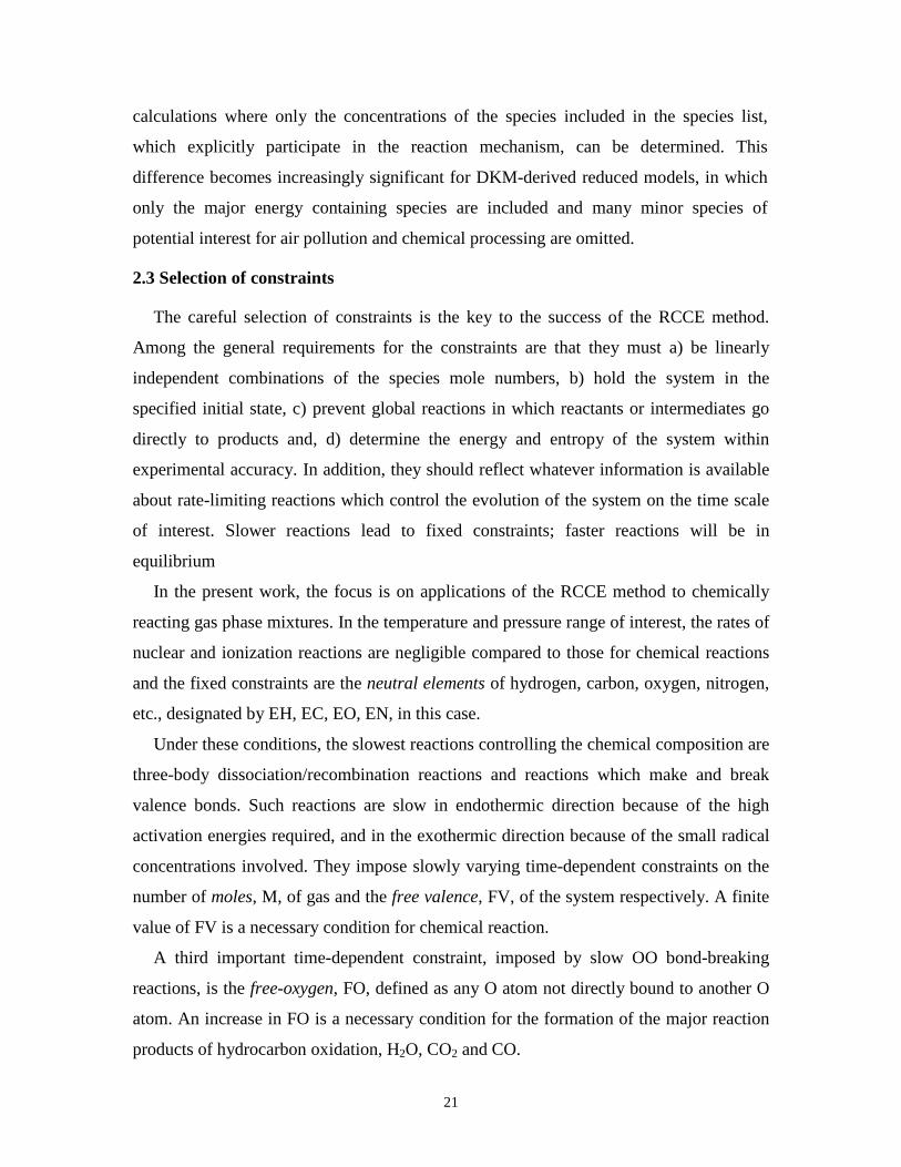
A third important time-dependent constraint, imposed by slow OO bond-breaking
reactions, is the free-oxygen, FO, defined as any O atom not directly bound to another O
atom. An increase in FO is a necessary condition for the formation of the major reaction
products of hydrocarbon oxidation, H2O, CO2 and CO.
22
Two additional time-dependent constraints which have been found useful for RCCE
calculations are: OHO≡OH+O and DCO≡HCO+CO. The former is a consequence of
the relatively slow OHO changing reaction RH+OH↔H2O+R coupled with the fast
reaction RH+O=OH+R which equilibrates OH and O. The later is a consequence of the
slow spin-forbidden reaction CO+HO2↔CO2+OH coupled with the fast reaction
HCO+O2=CO+HO2 which equilibrates HCO and CO.
The 8 constraints EH, EO, EC, M, FV, FO, OHO, and DCO are problem independent
and may therefore be considered “universal” constraints. Along with the equilibrium
reactions
H2+O=OH+H (CE1)
H2+HOO=H2O2+H (CE2)
HCO+O2=CO+HO2 (CE3)
they are sufficient to determine the constrained-equilibrium mole fractions of the fuel and
the 10 major hydrocarbon combustion products H, O, OH, HO2, H2, O2, H2O, H2O2, CO
and CO2.
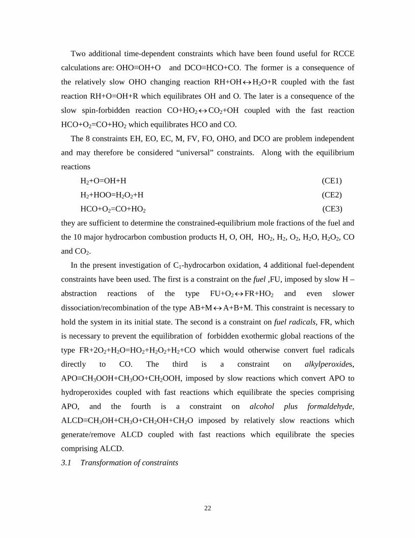
In the present investigation of C1-hydrocarbon oxidation, 4 additional fuel-dependent
constraints have been used. The first is a constraint on the fuel ,FU, imposed by slow H –
abstraction reactions of the type FU+O2↔FR+HO2 and even slower
dissociation/recombination of the type AB+M↔A+B+M. This constraint is necessary to
hold the system in its initial state. The second is a constraint on fuel radicals, FR, which
is necessary to prevent the equilibration of forbidden exothermic global reactions of the
type FR+2O2+H2O=HO2+H2O2+H2+CO which would otherwise convert fuel radicals
directly to CO. The third is a constraint on alkylperoxides,
APO≡CH3OOH+CH3OO+CH2OOH, imposed by slow reactions which convert APO to
hydroperoxides coupled with fast reactions which equilibrate the species comprising
APO, and the fourth is a constraint on alcohol plus formaldehyde,
ALCD≡CH3OH+CH3O+CH2OH+CH2O imposed by relatively slow reactions which
generate/remove ALCD coupled with fast reactions which equilibrate the species
comprising ALCD.
3.1 Transformation of constraints

23
The integration of equations (1.10) and (1.11) for the constraint-potentials requires
inversion of the Γ
C matrix. The performance of the implicit integrators, such as DASSL,
are quite sensitive to the structure of this matrix. In general, the codes work best when the
large elements of the matrix lie on or close to the main diagonal. This is not usually the
case for the initial set of constraints chosen and a variety of error messages such as
“singular matrix” or “failure to converge” may be encountered. The problem can almost
always be solved by a transformation of the square sub-matrix relating the major species
and the constraints to a diagonalized form. The physical meaning of the transformed
matrix may not be clear in all cases but if it improves the speed and reliability of the
integrator, the desired objective will have been achieved. In this connection, it is
important to note that any linear combination of the original linearly independent
constraints for which the integrator works should give the same final result. This can be a
useful check on the numerical results.
A general transformation of the constraint matrix can be made as follows. Assume G
is a square transformation matrix of order nc. Multiplying equation (1.2) through by this
matrix yields
NACGC~~
== (1.12)
where
AGA =~
(1.13)
is the transformed spc nn × constraint matrix that relates the transformed constraint
vector, ~
C , to the species vector, N. The corresponding transformation for the reaction
matrix is
BGB =~ (1.14)
The transformation equations for the constraint potentials can be obtained by noting that
the Gibbs free energy,cµ , is invariant under the transformation. Equation (4) then gives

24
( ) ~~~~ γγγγµ TTTTTc GAAGAA ====− (1.15)
Multiplying Equation (15) by A we obtain
γγµ ~Tc GSSA ==− (1.16)
where
TAAS = (1.17)
is a symmetric matrix of order nc. Assuming that S is non-singular, it follows from
Equation (16) that
γγ ~TG= (1.18a)
and, since G is non-singular,
γγ 1)(~ −= TG (1.18b)
2.4 Determination of initial conditions
For systems initially in a constrained-equilibrium state, the initial values of the
constraint potentials are finite. However, for a system initially in a non-equilibrium state,
where the concentrations of one or more species is zero, it can be seen from equation
(1.3) and (1.4) that one or more constraint-potentials must be infinite. This condition is
encountered in ignition-delay-time calculations, where the system is initially far from
equilibrium and the initial concentrations of all species except the reactants are assumed
to be zero.
One method of dealing with this problem is to assign small partial pressures to as
many major product species as required to give finite values for the constraint potentials.
Ideally the choice should be made in such a way that the partial pressures of all other
product species will be smaller than the assigned partial pressures. A reasonable initial

25
choice for a major species corresponding to a constraint is the one with the minimum
standard Gibbs free energy in the group of species included in the constraint.
To implement this method, equation (1.2) is decomposed in the form
[ ]
==
2
1
1211 N
NAANAC (1.19)
where 11
A is an cc nn × non-singular, square matrix giving the contribution of the major
species vector, 1N , to the constraint vector, C, and 12
A is an )( csc nnn −× matrix, giving
the contribution of 2N to C. The corresponding decomposition of equation (1.4) is
γγµ
µµ
−=−=
=
T
T
T
A
AA
12
11
2
1 (1.20)
Initial values for the constraint potentials can now be obtained by assuming
1µ (0)>>
2µ (0). This gives
01
1111
111 )0((ln)()0()()0( µµγ +−=−= −− pAA TT ) (1.21)
Having determined the initial values of the constraint-potential vector, one can now
check the assumption that the initial partial pressures of the minor species are small
using the relation
0
2122)0()0(ln µγ −−= TAp (1.22)
If they are not, an alternative choice for the major species will usually solve the problem.
In initial RCCE calculations using constraints based on kinetic considerations,
problems involving the convergence of the implicit integrators used were frequently
encountered. These were caused primarily by the fact the Γ
C matrix in equation (1.11)
contained large off diagonal elements. These problems were solved by a transformation
which diagonalized the 11
A matrix. Using the transformation matrix 1
11
−= AG we obtain
from equation (1.12)

26
[ ] [ ] NAN
NAAI
N
NAAACAC
~
2
1
12
1
11112
1
1211
1
11
1
11
~
=
=
== −−− (1.23)
and it follows from equation (1.15) that
)0(~)0()0(ln)0(~
11
0
11γγµµ −=−=+= Ip (1.24)
It can be seen from this equation, that in the diagonalized representation, the initial
constraint potentials are simply the initial Gibbs free energies of the major species chosen
as surrogates. The transformed reaction rate matrix is
BAB 111
~−= (1.25)
2.5 RCCE calculations for C1 hydrocarbon oxidation
To illustrate the RCCE method, we consider the homogeneous stoichiometric
oxidation of three mono-carbon fuels, namely methane (CH4), methanol (CH3OH) and
formaldehyde (CH2O) with pure oxygen in a constant volume reactor over a wide range
of initial temperatures (900K-1500K) and pressures (1atm-100atm). The 12 constraints
used in the RCCE calculations are summarized in Table 1.
The DKM calculations with which the RCCE results are compared involve only C1
chemistry and include 29 species and 133 reactions, without nitrogen chemistry. Twenty
species and 102 reactions were taken from the widely known and used GRI-Mech3.0 [21]
mechanism. This model does not include alkyl peroxides and therefore is not expected to
be valid under high-pressure low-temperature conditions. To obtain a model valid under
these conditions an additional 9 alkyl peroxides and organic acids were included along
with 31 reactions with rates taken from [22] or estimated by the authors.
Of the 133 reactions employed in the DKM calculations only 102 reactions change
one or more constraints of the constraints in Table 1 and are therefore of interest. The
remaining 31 are in constrained-equilibrium and are therefore redundant in RCCE
calculations, in principle, only the fastest reaction in a group which changes a given
constraint is required for a system to go from the specified initial state to the correct final

27
chemical-equilibrium state. However in practice, it is usually necessary to include
additional reactions to achieve the desired accuracy for the time-evolution of the system.
In this work, excellent agreement between DKM calculations and RCCE calculations was
obtained for all C1 species using 12 constraints and 102 reactions and acceptable
agreement was obtained using 12 constraints and 20 reactions for methane, 10 constraints
and 16 reactions for methanol, and 9 constraints and 12 reactions for formaldehyde.
1.5.1 Methane (CH4) Oxidation
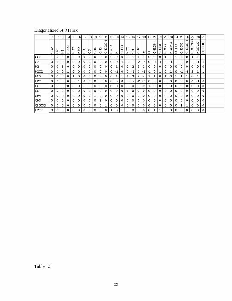
The constraint matrix for CH4 used in this work is shown in Table 2a and the
corresponding diagonalized matrix used to set the initial conditions and carry out the
numerical calculations is shown in Table 2b. Diagonalized 12 constraints and 29 species
are included. The corresponding RCCE reaction flow diagram is shown in figure 1.1. The
constrained species are enclosed by dashed lines. Except for the initiation steps, this
diagram also includes the sub-mechanisms involved in the oxidation of CH3OH and
CH2O.
As can be seen, the oxidation process is initiated by the highly endothermic CH4
constraint changing H-abstraction reaction
CH4+O2↔CH3+HO2 (RC1)
This is followed by the two competing CH3 constraint-changing reactions
CH3+O2+M ↔CH3OO+M (RC2)
CH3+O2↔CH3O+O (RC3)
The first is most important at low temperatures and is followed by the constrained-
equilibrium reactions
CH3OO+H2O2=CH3OOH+HO2 (CE1)
CH3OOH+HO2=CH2OOH+H2O2 (CE2)
which equilibrate the alkylperoxides in APO. The second is most important at high
temperatures and is followed by the constrained-equilibrium reactions
H2+O=OH+H (CE3)
which equilibrates the water radicals in OHO, and constrained-equilibrium reactions

28
CH3O+ H2O2=CH3OH+ HO2 (CE4)
CH3OH+HO2=CH2OH+H2O2 (CE5)
CH3O+O2=CH2O+HO2 (CE6)
which equilibrate the free oxygen species in ALCD. The CH4 constraint-changing
reaction
OH+CH4↔CH3+H2O (RC4)
converts OH in OHO to the product H2O and regenerates CH3.
The stable intermediate CH2O in ALCD is oxidized by the constraint-changing H-
abstraction reaction
CH2O+O2↔CHO+HO2 (RC5)
and the constrained-equilibrium reaction and the fast equilibrium reaction
CHO+O2=CO+HO2 (CE7)
to form DCO. The CO in DCO is converted to the product CO2 by the FO constraint-
changing reaction
CO+HO2↔CO2+OH (RC6)
Finally the 8 major H/O species are determined by the 4 constraint-changing reactions
HO2↔H+O2 (RC7)
HO2+HO2↔H2O2+O2 (RC8)
HO2+H↔OH+OH (RC9)
H+O2↔OH+O (RC10)
which change M, FV, FO, and OHO respectively, plus the 2 constrained-equilibrium
reactions
H2+O=OH+H (CE3)
H2+HO2=H2O2+H (CE8)
and the elemental constraints EH and EO.
As the above reactions proceed, the radical population increases rapidly and all
constraint-changing reactions included in the kinetic model become involved in
determining the evolution of the system and its approach to final chemical-equilibrium.
Of particular importance are reactions of the type
CH4+Q↔CH3+HQ (RC1.1)

29
and
CH2O+Q↔CHO+HQ (RC5.1)
where Q can be any radical, e.g. HO2, OH, H, O.
1.5.2 CH4 Results for Full 133 Reaction Set
Time-dependent temperature profiles of stoichiometric mixtures of methane and
oxygen at initial temperatures of 900K and 1500K and different initial pressures are
shown in figure 1.2. All 12 constraints listed in Table 2 have been included. As
previously noted, only 102 of the reactions in the full set of 133 reactions change
constraints and are therefore required. The remaining 31 are in constrained-equilibrium
and are redundant in RCCE calculations.
It can be seen that the agreement with DKM calculations is excellent over the entire
range of pressure and temperature covered. Note that the temperature overshoot at low
pressures due to slow three-body recombination and dissociation reactions is well
reproduced by the constraint M on the total moles. Also, the same comparisons have been
made for rich ( 2.1=φ ) and lean ( 8.0=φ ) mixtures in figure 1.3. RCCE predictions of
ignition delay times at low temperature, high pressure are within 1% of those by DKM.
At high temperature, low pressure the results agree within 1%-5% of accuracy.
More complete results are shown on log-log plots in figure 1.4 for the initial
conditions 900 K, 100 atm, where the dominant radicals are HO2≈CH3 at early times and
CH3OO at late times, and in figure 1.5 for the initial conditions 1500 K, 1atm, where the
dominant radicals are HO2≈CH3OO at all times. As can be seen in figures 1.3a and 1.4a,
the temperature first decreases due to the fact that the initiation reactions are all
endothermic then later increases as exothermic reactions become important. The
agreement between RCCE and DKM calculations, especially with regard to the time at
which the temperature difference becomes positive, is excellent.
Figures 1.3b and 1.4b show the time dependence of the constraint-potentials for the
diagonalized constraint-matrix and figures 1.3c and 1.4c show the corresponding
constraint-potentials for the original constraint matrix. Note that for the original
constraint matrix, all the time-dependent constraint-potentials go to zero at equilibrium as

30
required, while those for the elements go to values identical with those obtained from the
STANJAN equilibrium code [23]. Once the constraint-potentials have been determined,
the constrained–equilibrium mole fractions of any species for which the standard Gibbs
free energy is known can be calculated from Equation (3).
The fixed elemental constraints and the most important time-dependent constraints
M, FV, FO, FU and FR are shown in figures 1.3d and 1.4d and the mole fractions of the
major species are shown in figures 1.3e-h and 1.4e-h. It can be seen that overall
agreement is very good.
To investigate the sensitivity of the ignition delay time to the number of constraints
used, a series of RCCE calculations was carried out starting with the 8 constraints EH,
EC, EO, M, FV, FO, OHO FU and adding additional constraints one at a time. The
results for both high and low temperature conditions are compared with those of the
DKM in figure 1.6. It can be seen that for high temperature conditions, 9 constraints are
sufficient to give the agreement within 5%, while for low temperature conditions, 11
constraints are required to give the same agreement.
5.1.2 Reduced CH4 reaction mechanism
In the initial studies, a full set of 133 reactions was used for both the RCCE and DKM
calculations. Clearly not all of these are of equal importance especially in RCCE
calculations where, in principle, only one independent reaction for each time-dependent
constraint is required to allow the system to relax from the specified initial state to the
correct final chemical-equilibrium state. In general, however, this does not give the
correct time evolution of the system and additional reactions are required to achieve the
desired degree of accuracy.
By systematically eliminating unimportant reactions, a reduced mechanism for C1
hydrocarbons involving the 24 constraint-changing reactions in Table 3 has been found.
The minimum set of reactions required for the individual fuels: CH4, CH3OH and CH2O,
are indicated by cross marks in the left columns of the Table. The constraints required for
each one of the fuels are indicated by cross marks in the top rows of the Table. Arrhenius
31
rate-parameters and uncertainty factors taken from Tsang and Hampson [22] are also
shown in the right hand columns of the Table. It can be seen that many of the rates have
estimate uncertainties greater than a factor of 3 even though these are among the simplest
and best known reactions. For each constraint where more than one reaction is listed, the
redundant reactions are important at different stages in the evolution of the system.
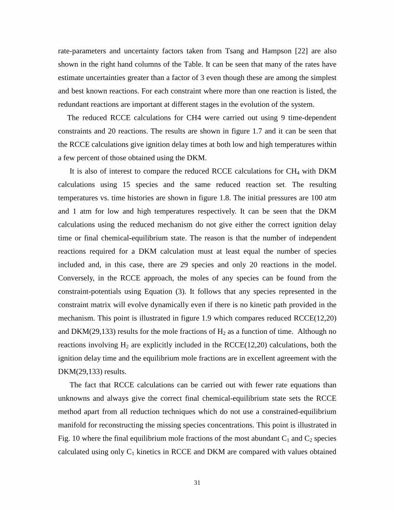
The reduced RCCE calculations for CH4 were carried out using 9 time-dependent
constraints and 20 reactions. The results are shown in figure 1.7 and it can be seen that
the RCCE calculations give ignition delay times at both low and high temperatures within
a few percent of those obtained using the DKM.
It is also of interest to compare the reduced RCCE calculations for CH4 with DKM
calculations using 15 species and the same reduced reaction set. The resulting
temperatures vs. time histories are shown in figure 1.8. The initial pressures are 100 atm
and 1 atm for low and high temperatures respectively. It can be seen that the DKM
calculations using the reduced mechanism do not give either the correct ignition delay
time or final chemical-equilibrium state. The reason is that the number of independent
reactions required for a DKM calculation must at least equal the number of species
included and, in this case, there are 29 species and only 20 reactions in the model.
Conversely, in the RCCE approach, the moles of any species can be found from the
constraint-potentials using Equation (3). It follows that any species represented in the
constraint matrix will evolve dynamically even if there is no kinetic path provided in the
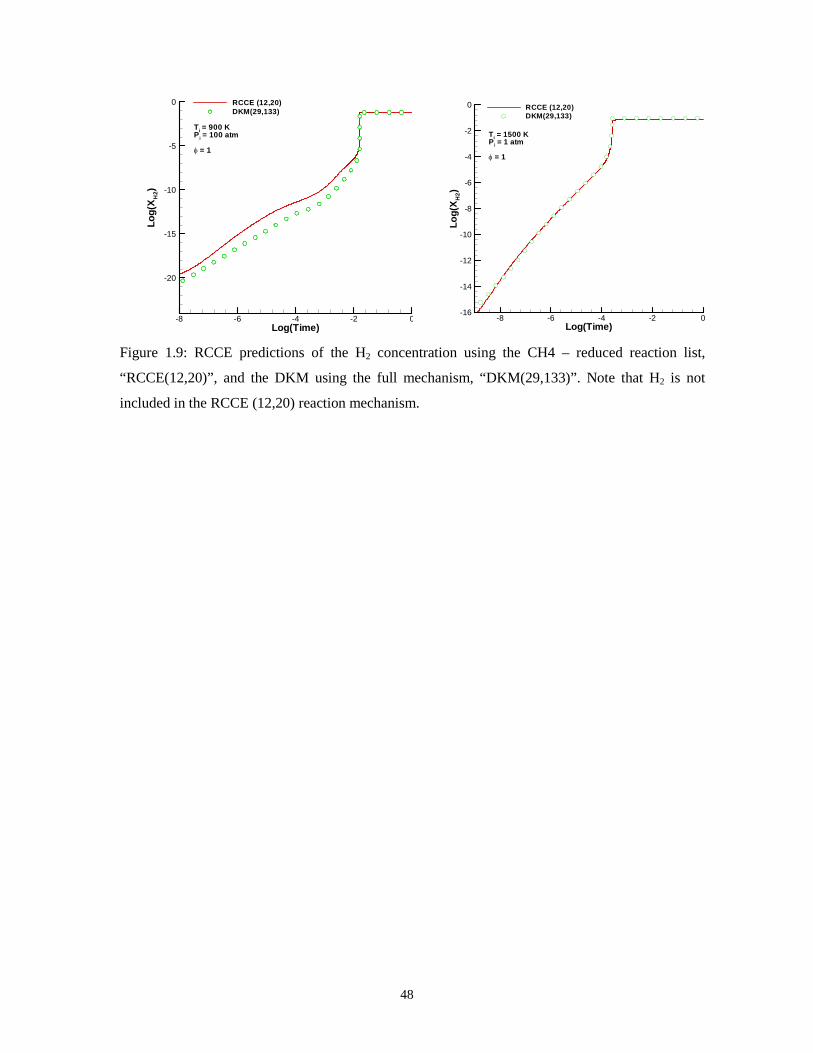
mechanism. This point is illustrated in figure 1.9 which compares reduced RCCE(12,20)
and DKM(29,133) results for the mole fractions of H2 as a function of time. Although no
reactions involving H2 are explicitly included in the RCCE(12,20) calculations, both the
ignition delay time and the equilibrium mole fractions are in excellent agreement with the
DKM(29,133) results.
The fact that RCCE calculations can be carried out with fewer rate equations than
unknowns and always give the correct final chemical-equilibrium state sets the RCCE
method apart from all reduction techniques which do not use a constrained-equilibrium
manifold for reconstructing the missing species concentrations. This point is illustrated in
Fig. 10 where the final equilibrium mole fractions of the most abundant C1 and C2 species
calculated using only C1 kinetics in RCCE and DKM are compared with values obtained

32
using the STANJAN equilibrium code. For C1 species, all values agree perfectly.
However for C2 species, the RCCE and STANJAN values agree but the DKM values are
unchanged from their original assigned values for the obvious reason that the C1 kinetics
used in the DKM does not include any reactions which change C2 species.
1.5.3 Methanol (CH3OH) Oxidation
The same set of basic constraints used for CH4 can be used for the oxidation of
methanol. However in this case, the fuel molecule FU is CH3OH and fuel radical
constraint, FR, is CH3O+CH2OH+CH2O. In addition, an examination of the kinetics
shows that alkylperoxydes reactions are not important and the APO constraint can be
eliminated. This results in a reduction of the total number of constraints from 12 to 10.
The corresponding reaction diagram is shown in Fig 11.
1.5.4 Reduced CH3OH reaction mechanism
A reduced set of 16 reactions for CH3OH oxidation is included in Table 3. RCCE
calculations using these 16 reactions and the 7 time-dependent constraints included in
Table 3 are compared with DKM calculations using 133 reactions and 29 species in
figure 1.12. It can be seen that the temperature vs. time plots are in excellent agreement
over the entire range of temperature and pressure covered. The agreement for all other
variables is similar to that for CH4.
1.5.5 Formaldehyde (CH2O) Oxidation
The reaction diagram for CH2O oxidation is shown in figure 1.13 and a reduced
kinetic model is included in Table 3. The reduced kinetic model in this case is even
simpler than that for CH3OH and only 9 constraints and 12 reactions are required in the
RCCE calculations. A comparison of temperature versus time plots is shown in figure
1.14 and again it can be seen that the agreement between RCCE and DKM calculations is
33
excellent. As in the case of CH3OH, plots of all other variables are also in excellent
agreement and are similar to those for CH4.
2.6 Summary and conclusions
RCCE calculations of methane, methanol and formaldehyde oxidation over a wide
range of initial temperatures and pressures have been made using up to 12 constraints and
133 reactions and excellent agreement with “detailed”-kinetic-model (DKM) calculations
using 29 species and the same reactions have been obtained. In addition, reduced sets of
20 reaction for methane, 12 reactions for methanol and 12 reactions for formaldehyde
have been found, which when employed in the RCCE calculations give results identical
to those obtained using the full 133 reactions.
Among the important features of the RCCE method for simplifying the kinetics of
hydrocarbon oxidation are:
1. It is based on the well established Maximum Entropy Principle of
thermodynamics rather than mathematical approximations.
2. The entropy always increases as the system evolves and an approach to the
correct final chemical-equilibrium state for the specified elements is
guaranteed. This is not true for DKMs where only the listed species are
included and all others are missing.
3. The total number of constraints required to describe the state of a complex
chemical system can be very much smaller than the number of species in the
system resulting in fewer equations.
4. It enables one to obtain a good description of the kinetic behaviour of a
complex chemically reacting system using a relatively small number of
constraint-controlling reactions without having to start with a DKM.

34
5. An estimate of the concentrations of any species for which the standard Gibbs
free energy is known can be obtained even though the species is not explicitly
included in the model used.
6. If the only constraints on the system are the elements and the state variables,
RCCE calculations reduce to local equilibrium (LTE) calculations.
7. If the species are used as constraints, RCCE calculations simulate DKM
calculations with the important distinction that only the listed species can
appear in DKM calculations whereas all possible species are implicitly
included in RCCE calculations.
8. The accuracy of the results can be systematically improved by adding
constraints one at a time.
2.7 Acknowledgment
This work was partially supported by ARO under technical monitoring of Dr. Ralph
Anthenion.
2.8 References
[1] S. W. Benson, J. Chem. Phys. 20, (1952) 1605
[2] Rein, M. Phys. Fluids A, 4 (1992) 873
[3] Mass, U., and Pope, S.B., Combust. Flame 88 (1992) 239
[4] Lam, S.H. and Goussis, D.A., Proc. Combust. Inst. 22 (1988) 931.
[5] Oluwayemisi O. Oluwole, Binita Bhattacharjee, John E. Tolsma, Paul I. Barton,
and William H. Green, Combust. Flame, 146, 1-2, 2006, p. 348-365.
35
[6] Lu, T., and Law, C. K., Combust. Flame, 144, (1-2) (2006) 24-36.
[7] Ren, Z.; Pope, S. B.; Vladimirsky, A.; Guckenheimer, J. M. J. ``The ICE-PIC
method for the dimension reduction of chemical kinetics'', Chem. Phys., 124, Art.
No. 114111, 2006
[8] Keck, J.C., and Gillespie, D., Combust. Flame, 17 (1971) 237.
[9] Law, R., Metghalchi, M. and Keck, J.C., Proc. Combust. Inst. 22 (1988) 1705.
[10] Bishnu, P., Hamiroune, D., Metghalchi, M., and Keck, J.C., Combustion Theory
and Modelling, 1 (1997) 295-312
[11] Hamiroune, D., Bishnu, P., Metghalchi, M. and Keck, J.C., Combustion Theory
and Modelling, 2 (1998) 81
[12] Yousefian V. A. Rate-Controlled Constrained-Equilibrium Thermochemistry
Algorithm for Complex Reacting Systems, Combustion and Flame 115, 66-80,
1998
[13] Tang, Q., and Pope, S. B., “A more accurate projection in the rate-controlled
constrained-equilibrium method for dimension reduction of combustion
chemistry,”' Combustion Theory and Modelling, 255-279, 2004.
[14] Jones, W.P. and Rigopoulos, S., Rate-controlled Constrained Equilibrium:
Formulation and Application of Non-Premixed Laminar Flames, Combustion and
Flame, 142, 223-234, 2005.
[15] Jones, W.P. and Rigopoulos, S., Reduced Chemistry for Hydrogen and Methanol
Premixed Flames via RCCE, Combustion Theory and Modeling, 11, 5, 755-780,
2007.
[16] Keck, J.C., Prog. Energy Combust. Sci., 16 (1990) 125
[17] Bishnu, P. S., Hamiroune, D., Metghalchi, M., “Development of Constrained
Equilibrium Codes and Their Applications in Nonequilibrium Thermodynamics”,
J. Energy Resour. Technol., Vol 123, Issue 3, 214, 2001
[18] Gao, Y., “Rate Controlled Constrained-Equilibrium Calculations of
Formaldehyde Oxidation” PhD Thesis, Northeastern University, Boston, 2003.
36
[19] Ugarte, S., Gao, Y., Metghalchi, H., Int. J. Thermodynamics, 3 (2005) 21
[20] Petzold, L., SIAM J., Sci. Stat. Comput. 3:367 (1982)
[21] Http://www.me.berkeley.edu/gri-mech/version30/text30.html.
[22] Tsang, W., Hampson, R. F., J. Phys. Chem. Ref. Data, 15 (3) (1986) 1087-1193.
[23] Reynolds, W. C., STANJAN Program, Stanford University, ME270, HO#7
Table 1.1

37
Definition of the Constraints
Constraint Definition of the Constraint
1 EC Elemental carbon
2 EO Elemental oxygen
3 EH Elemental hydrogen
4 M Total number of moles
5 FV Moles of free valance (any unpaired valence electron)
6 FO Moles of free oxygen (any oxygen not directly attached to another oxygen)
7 OHO Moles of water radicals (O+OH)
8 DCO Moles of HCO+CO
9 FU Moles of fuel molecule (CH4 in the case of Methane)
10 FR Moles of fuel radical(s) (CH3 in the case of Methane)
11 APO Moles of AlkyPerOxydes (CH3OO+CH3OOH+CH2OOH)
12 ALCD Moles of Alcohols+Aldehydes (CH3O+CH3OH+CH2OH+CH2O)

38
Table 1.2a
Constraint Matrix A for the C1 system
1 2 3 4 5 6 7 8 9 10 11 12 13 14 15 16 17 18 19 20 21 22 23 24 25 26 27 28 29
CO
2
O2
H2
H2O
2
HO
2
H2O
HO
CO
CH
4
CH
3
CH
3OO
H
H2C
O
H CH
3O
HC
O
CH
CH
2
C O CH
2OH
CH
3OH
HO
CO
HO
CH
O
OC
HO
CH
3OO
CH
2OO
H
HO
OC
HO
HO
OC
O
OO
CH
O
EC 1 0 0 0 0 0 0 1 1 1 1 1 0 1 1 1 1 1 0 1 1 1 1 1 1 1 1 1 1
EO 2 2 0 2 2 1 1 1 0 0 2 1 0 1 1 0 0 0 1 1 1 2 2 2 2 2 3 3 3
EH 0 0 2 2 1 2 1 0 4 3 4 2 1 3 1 1 2 0 0 3 4 1 2 1 3 3 2 1 1
M 1 1 1 1 1 1 1 1 1 1 1 1 1 1 1 1 1 1 1 1 1 1 1 1 1 1 1 1 1
FV 0 0 0 0 1 0 1 0 0 1 0 0 1 1 1 3 2 4 2 1 0 1 0 1 1 1 0 1 1
FO 2 0 0 0 0 1 1 1 0 0 0 1 0 1 1 0 0 0 1 1 1 2 2 2 0 0 1 1 1
OHO 0 0 0 0 0 0 1 0 0 0 0 0 0 0 0 0 0 0 1 0 0 0 0 0 0 0 0 0 0
DCO 0 0 0 0 0 0 0 1 0 0 0 0 0 0 1 0 0 0 0 0 0 0 0 0 0 0 0 0 0
FU 0 0 0 0 0 0 0 0 1 0 0 0 0 0 0 0 0 0 0 0 0 0 0 0 0 0 0 0 0
FR 0 0 0 0 0 0 0 0 0 1 0 0 0 0 0 0 0 0 0 0 0 0 0 0 0 0 0 0 0
APO 0 0 0 0 0 0 0 0 0 0 1 0 0 0 0 0 0 0 0 0 0 0 0 0 1 1 0 0 0
ALCD 0 0 0 0 0 0 0 0 0 0 0 1 0 1 0 0 0 0 0 1 1 0 0 0 0 0 0 0 0
Table 1.2b
39
Diagonalized A Matrix 1 2 3 4 5 6 7 8 9 10 11 12 13 14 15 16 17 18 19 20 21 22 23 24 25 26 27 28 29
CO
2
O2
H2
H2O
2
HO
2
H2O
HO
CO
CH
4
CH
3
CH
3OO
H
H2C
O
H CH
3O
HC
O
CH
CH
2
C O CH
2OH
CH
3OH
HO
CO
HO
CH
O
OC
HO
CH
3OO
CH
2OO
H
HO
OC
HO
HO
OC
O
OO
CH
O
CO2 1 0 0 0 0 0 0 0 0 0 0 0 0 0 0 1 1 1 0 0 0 1 1 1 0 0 1 1 1
O2 0 1 0 0 0 0 0 0 0 0 0 0 0 -1 -1 -2 -2 -2 0 -1 -1 -1 -1 -1 0 0 -1 -1 -1
H2 0 0 1 0 0 0 0 0 0 0 0 0 1 0 0 2 2 2 0 0 0 0 0 0 0 0 0 0 0
H2O2 0 0 0 1 0 0 0 0 0 0 0 0 -1 0 0 -1 0 -2 -1 0 1 0 1 0 -1 -1 2 1 1
HO2 0 0 0 0 1 0 0 0 0 0 0 0 1 1 1 3 2 4 1 1 0 1 0 1 1 1 0 1 1
H2O 0 0 0 0 0 1 0 0 0 0 0 0 0 0 0 -2 -2 -2 0 0 0 0 0 0 0 0 -1 -1 -1
HO 0 0 0 0 0 0 1 0 0 0 0 0 0 0 0 0 0 0 1 0 0 0 0 0 0 0 0 0 0
CO 0 0 0 0 0 0 0 1 0 0 0 0 0 0 1 0 0 0 0 0 0 0 0 0 0 0 0 0 0
CH4 0 0 0 0 0 0 0 0 1 0 0 0 0 0 0 0 0 0 0 0 0 0 0 0 0 0 0 0 0
CH3 0 0 0 0 0 0 0 0 0 1 0 0 0 0 0 0 0 0 0 0 0 0 0 0 0 0 0 0 0
CH3OOH 0 0 0 0 0 0 0 0 0 0 1 0 0 0 0 0 0 0 0 0 0 0 0 0 1 1 0 0 0
H2CO 0 0 0 0 0 0 0 0 0 0 0 1 0 1 0 0 0 0 0 1 1 0 0 0 0 0 0 0 0
Table 1.3
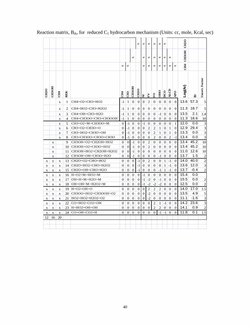
40
Reaction matrix, Bik, for reduced C1 hydrocarbon mechanism (Units: cc, mole, Kcal, sec)
x
x
x
x
x
x
CH
2O
x
x
x
x
x
x
x
CH
3O
H
x
x
x
x
x
x
x
x
x
CH
4
CH
2O
CH
3O
H
CH
4
RE
K
CH
4
CH
3
CH
3O
H
CH
2O
M FV
FO
OH
O
DC
O
ALC
D
AP
O
Lo
g(A
r)
Er
Unc
ert. F
act
or
x 1 CH4+O2=CH3+HO2 -1 1 0 0 0 2 0 0 0 0 0 13.6 57.3 5
x 2 CH4+HO2=CH3+H2O2 -1 1 0 0 0 0 0 0 0 0 0 11.3 18.7 5
x 3 CH4+OH=CH3+H2O -1 1 0 0 0 0 0 -1 0 0 0 13.5 2.1 1.4x 4 CH4+CH3OO=CH3+CH3OOH -1 1 0 0 0 0 0 0 0 0 0 11.3 18.6 10x 5 CH3+O2+M=CH3OO+M 0 -1 0 0 -1 0 0 0 0 0 1 12.0 0.0 3x 6 CH3+O2=CH3O+O 0 -1 0 0 0 2 2 1 0 1 0 12.9 29.4 3x 7 CH3+HO2=CH3O+OH 0 -1 0 0 0 0 2 1 0 1 0 13.3 0.0 3x 8 CH3+CH3OO=CH3O+CH3O 0 -1 0 0 0 0 2 0 0 2 -1 13.4 0.0 3
x 9 CH3OH+O2=CH2OH+HO2 0 0 -1 0 0 2 0 0 0 0 0 13.4 45.2 10x 10 CH3OH+O2=CH3O+HO2 0 0 -1 0 0 2 0 0 0 0 0 13.4 45.2 10x 11 CH3OH+HO2=CH2OH+H2O2 0 0 -1 0 0 0 0 0 0 0 0 11.0 12.6 10x 12 CH3OH+OH=CH3O+H2O 0 0 -1 0 0 0 0 -1 0 0 0 13.7 1.5 2
x x x 13 CH2O+O2=CHO+HO2 0 0 0 -1 0 2 0 0 1 -1 0 14.0 40.0 2x x x 14 CH2O+HO2=CHO+H2O2 0 0 0 -1 0 0 0 0 1 -1 0 13.6 12.0 3x x x 15 CH2O+OH=CHO+H2O 0 0 0 -1 0 0 0 -1 1 -1 0 13.7 -0.4 2x x x 16 H+O2+M=HO2+M 0 0 0 0 -1 0 0 0 0 0 0 15.4 0.0x x x 17 OH+H+M=H2O+M 0 0 0 0 -1 -2 0 -1 0 0 0 15.5 0.0 2x x x 18 OH+OH+M=H2O2+M 0 0 0 0 -1 -2 -2 -2 0 0 0 12.5 0.0 2x x x 19 H+O2=OH+O 0 0 0 0 0 2 2 2 0 0 0 14.0 17.0 1.5x x x 20 CH3OO+HO2=CH3OOH+O2 0 0 0 0 0 -2 0 0 0 0 0 13.5 4.9 5x x x 21 HO2+HO2=H2O2+O2 0 0 0 0 0 -2 0 0 0 0 0 11.1 -1.6 3x x x 22 CO+HO2=CO2+OH 0 0 0 0 0 0 2 1 -1 0 0 14.2 23.6 3x x x 23 H+HO2=OH+OH 0 0 0 0 0 0 2 2 0 0 0 14.1 0.9 2x x x 24 CO+OH=CO2+H 0 0 0 0 0 0 0 -1 -1 0 0 11.8 0.1 1.5
12 16 20

41
Figure 1.1: RCCE reaction flow diagram for CH4 oxidation.
CH4
O2 HO2 H2O2
H
O2
O
OH
..
.
.
.
CH3
O2
CH3OO
O
CH3O CH3OH
CH2OH
OH
H2O
CH4
.
. ..
.
. CH3OOH
.
CO
CH2OOH
O2
.
CH2O
CHO .
HO2 .
OH
CO2
HO2 .
1
2
3 4
5
6
7
8
9
10
.

42
Time (ms)
Tem
per
atu
re(K
)
14 15 16 17 181000
2000
3000
4000
5000 RCCE, φ = 1.2DKM, φ = 1.2RCCE, φ = 1.0DKM, φ = 1.0RCCE, φ = 0.8DKM, φ = 0.8
φ = 0.8
φ = 1.2
φ = 1.0
Time (ms)
Tem
per
atu
re(K
)
0.2 0.25 0.3
1500
2000
2500
3000
3500
4000RCCE, φ = 0.8DKM, φ = 0.8RCCE, φ = 1.0DKM, φ = 1.0RCCE, φ = 1.2DKM, φ = 1.2
Figure 1.3: Temperature profiles for mixtures of CH4/O2 at different equivalence ratios at initial
pressure and temperature of 100 atm and 900K, (a), and 1 atm and 1500 K (b).
Log(Time)
Tem
pera
ture
(K)
-4 -3 -2 -1 0 1
1000
1500
2000
2500
3000
3500
4000
4500RCCEDetailed
P=100 atm
P=1atm
P=10 atmP=50 atm
Log(Time)
Tem
per
atu
re(K
)
-7 -6 -5 -4 -3
1500
2000
2500
3000
3500
4000
4500RCCEDetailed
P=100 atm
P=1atm
P=10 atm
P=50 atm
Figure 1.2: Temperature profiles at different initial pressures for stoichiometric mixture of
CH4/O2 at initial temperatures of 900 K (a), and 1500 K (b).
(a) (b)
DKM DKM
(a) (b)

43
Log(Time)
Log|
T-T
i|
-10 -8 -6 -4 -2 0
-10
-5
0
5RCCE (12,113)DKM(29,133)
T > TiT < Ti
Log(Time)
Log
(Mol
eF
ract
ion)
-10 -8 -6 -4 -2 0-14
-12
-10
-8
-6
-4
-2
0 O2
CO2
CH4
H2O
CO
Log(Time)
Dia
gon
alC
onst
rain
tPot
entia
ls
-10 -8 -6 -4 -2 00
20
40
60
80
100
120
O2
CO2
H2
H2O
CH4
HO2
H2O
H2
HO2
O2
CH3
CO2
H2O2
H2O2
CH4CH3
Log(Time)
Log
(Mol
eF
ract
ion)
-10 -8 -6 -4 -2 0
-14
-12
-10
-8
-6
-4
-2
0
CH2O
CH3
CH3OO
CH3OOH
CH3
CH3OOH
CH3OO
CH2O
Log(Time)
Co
nstr
ain
tPo
ten
tials
-10 -8 -6 -4 -2 0-150
-125
-100
-75
-50
-25
0
25
50
75
100
EC
FV
EH
M
FR
FO
FU
EH
EC
EO
Log(Time)
Log(
Mol
eF
ract
ion)
-10 -8 -6 -4 -2 0
-14
-12
-10
-8
-6
-4
-2
0
H
HO2
H2O2
OH
H
HO2
H2O2
H2
OH
Log(Time)
Log
(Con
stra
ints
)
-10 -8 -6 -4 -2 0
-12
-9
-6
-3
0
3
EH,EO
M
FU
EC
FR
FO
FV
FU
FR
Log(Time)
Log
(Mol
eF
ract
ion)
-10 -8 -6 -4 -2 0-14
-12
-10
-8
-6
-4
-2
0
OCHO
HOCO
HOCHO
Figure 1.4: RCCE versus DKM predictions of stoichiometric CH4/O2 auto-ignition at Ti = 900 K, Pi = 100 atm. Lines represent RCCE and symbols represent detailed kinetics.
(a)
(b)
(c)
(d)
(e)
(f)
(g)
(h)

44
Log(Time)
Log
|T-T
i|
-10 -8 -6 -4 -2
-10
-5
0
5RCCE (12,113)DKM(29,133)
T > TiT < Ti
Log(Time)
Lo
g(M
ole
Fra
ctio
n)
-10 -8 -6 -4 -2-14
-12
-10
-8
-6
-4
-2
0
O2
CO2 CH4
H2O CO
CH4
Log(Time)
Dia
gona
lCo
nstr
aint
Pot
entia
ls
-10 -8 -6 -4 -220
40
60
80
100
O2
CO2
H2
H2O
CH4
HO2
H2O
H2
HO2
O2
CH3
CO2
H2O2
H2O2
CH4CH3
Log(Time)
Log
(Mo
leF
ract
ion)
-10 -8 -6 -4 -2-18
-16
-14
-12
-10
-8
-6
-4
-2
0
CH3
CH2O
CH3OOH
CH3OO
CH3
CH2O
CH3OOH
CH
3OO
Log(Time)
Con
stra
intP
oten
tials
-10 -8 -6 -4 -2-125
-100
-75
-50
-25
0
25
50
EC
EOFV
EHM
FR
FO
FU
EH
EC
EO
Log(Time)
Log
(Mo
leF
ract
ion)
-10 -8 -6 -4 -2
-14
-12
-10
-8
-6
-4
-2
0H2
H2O2
HO2
OHH
HO2H2O2
H2
OH
H
Log(Time)
Log
(Co
nstr
aint
s)
-10 -8 -6 -4 -2 0
-12
-9
-6
-3
0
3
EH,EO
M
FU
EC
FR
FO
FV
FU
FR
Log(Time)
Log
(Mol
eF
ract
ion
)
-10 -8 -6 -4 -2-18
-16
-14
-12
-10
-8
-6
-4
-2
0
OCHO
HOCO
HOCHO
Figure 1.5: RCCE versus DKM predictions of stoichiometric CH4/O2 auto-ignition at Ti = 1500 K, Pi = 1 atm. Lines represent RCCE and symbols represent DKM.
(a)
(b)
(c)
(d)
(e)
(f)
(g)
(h)

45
0
0.005
0.01
0.015
0.02
0.025
0.03
9th = FR 10th = ALCD 11th = APO 12th = DCO
Ign
itio
n D
elay
Tim
e (s
ec)
(Ti=
900K
, Pi=
100
atm
)
RCCE DKM
0
0.0001
0.0002
0.0003
9th = FR 10th = ALCD 11th = APO 12th = DCO
Ign
itio
n D
elay
Tim
e (s
ec)
(Ti =
150
0 K
, Pi =
1at
m)
Series1 Series2
Figure 1.6: Constraint dependence study of ignition delay time predictions for stoichiometric CH4/O2 auto-ignition at different initial temperatures.

46
Log(Time)
Tem
pera
ture
(K)
-4 -3 -2 -1 0 1
1000
1500
2000
2500
3000
3500
4000
4500
5000 RCCE(12,20)DKM(29,133)
Pi = 1 atm
Pi = 100 atm
Pi = 10 atm
Log(Time)
Tem
pera
ture
(K)
-8 -6 -4 -2
1500
2000
2500
3000
3500
4000
4500
5000 RCCE(12,20)DKM(29,133)
Pi=1 atm
Pi=100 atm
Pi=10 atm
Figure 1.7: RCCE predictions of temperature profiles for Ti = 900 K and 1500 K at different initial
pressures using the reduced reaction mechanism listed in Table 3, “RCCE (12,20)”, compared with
the detailed kinetics model predictions using the original 133 reactions, “DKM(29,133)”.

47
Log(Time)
Tem
pera
ture
(K)
-4 -3 -2 -1
1000
1500
2000
2500
3000
3500
4000
4500 RCCE(12,20)DKM(15,20)DKM(29,133)
Log(Time)
Tem
pera
ture
(K)
-6 -5 -4 -3 -2
1500
2000
2500
3000
3500
4000 RCCE(12,20)DKM(15,20)DKM(29,133)
Figure 1.8: RCCE predictions of the temperature profiles for Ti = 900 K and 1500 K using the CH4 –
reduced reaction mechanism listed in Table 3, “RCCE (12,20)”, compared with the DKM predictions
using the original 29 species and 133 reactions, “DKM(29,133)”, and the DKM predictions using the
same reduced reaction mechanism, including 15 species and 20 reactions “DKM(15,20)”. The initial
pressures are 100 atm and 1atm for low and high temperature cases respectively.
48
Log(Time)
Log
(XH
2)
-8 -6 -4 -2 0
-20
-15
-10
-5
0 RCCE (12,20)DKM(29,133)
Ti = 900 KPi = 100 atm
φ = 1
Log(Time)
Log(
XH
2)
-8 -6 -4 -2 0-16
-14
-12
-10
-8
-6
-4
-2
0 RCCE (12,20)DKM(29,133)
Ti = 1500 KP i = 1 atm
φ = 1
Figure 1.9: RCCE predictions of the H2 concentration using the CH4 – reduced reaction list,
“RCCE(12,20)”, and the DKM using the full mechanism, “DKM(29,133)”. Note that H2 is not
included in the RCCE (12,20) reaction mechanism.

49
Figure 1.10: Comparison between final equilibrium calculations of the mole fractions of species, Log10(X i), using STANJAN, RCCE and DKM with C2 – species used in GRI-Mech3.0 added to species list, while using C1 – kinetic mechanism in kinetic calculations.
-35
-30
-25
-20
-15
-10 -5 0
H2O
CO
OH
H2
O2
HCO2
O
HO2
H2O2
HCO
HOCO
CH2O
HOCHO
C
CH
CH2
CH3
CH2OH
CH4
HCCO
CH3O
CH3OH
CH2CO
C2H2
OCHO
HOOCO
CH3OO
C2H
HCCOH
CH3OOH
CH2OOH
C2H3
CH3CHO
C2H4
OOCHO
HOOCHO
C2H5
C2H6
C3H7
C3H8
STA
NJA
N
RC
CE
Detailed
-30
-25
-20
-15
-10 -5 0
H2O
CO
OH
CO2
O2
H2
O
H
HO2
H2O2
HCO
HOCO
HOCHO
CH2O
CH2OH
C
CH3
CH2
CH
HCCO
CH4
CH3OH
CH3O
CH2CO
C2H2
CH3OO
HCCOH
CH3OOH
C2H
HOOCO
OCHO
CH2OOH
C2H3
CH3CHO
C2H4
C2H5
OOCHO
C2H6
HOOCHO
C3H7
C3H8
STA
NJA
N
RC
CE
Detailed
Ti = 900 K, Pi = 100 atm
Ti = 1500 K, Pi = 1 atm

50
Figure 1.11: RCCE reaction flow diagram of CH3OH/O2 auto-ignition.
CH3OH
O2
CO
O2
CHO
OH
.
HO2 .
.
CH3O CH2OH . .
CH2O
CO2
HO2 H2O2
H
O2
O
OH
..
.
.
.
. HO2
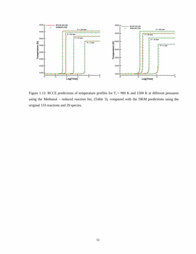
51
Log(Time)
Tem
per
atur
e(K
)
-4 -3 -2 -1 0 1
1000
1500
2000
2500
3000
3500
4000
4500 RCCE (10,16)DKM(29,133)
P = 50 atm
P = 1 atm
P = 10 atm
P = 100 atm
Log(Time)
Tem
per
atur
e(K
)
-8 -6 -4 -2
1500
2000
2500
3000
3500
4000
4500RCCE (10,16)DKM (29,133)
P = 100 atm
P = 1 atm
P = 10 atm
P = 50 atm
Figure 1.12: RCCE predictions of temperature profiles for Ti = 900 K and 1500 K at different pressures
using the Methanol – reduced reaction list, (Table 3), compared with the DKM predictions using the
original 133 reactions and 29 species.

52
Figure 1.13: RCCE reaction flow diagram of CH2O/O2 auto-ignition.
CH2O
O2
CO
CHO
HO2
.
HO .
CO2
HO2 H2O2
H
O2
O
OH
..
.
.
.
HO2 .
.
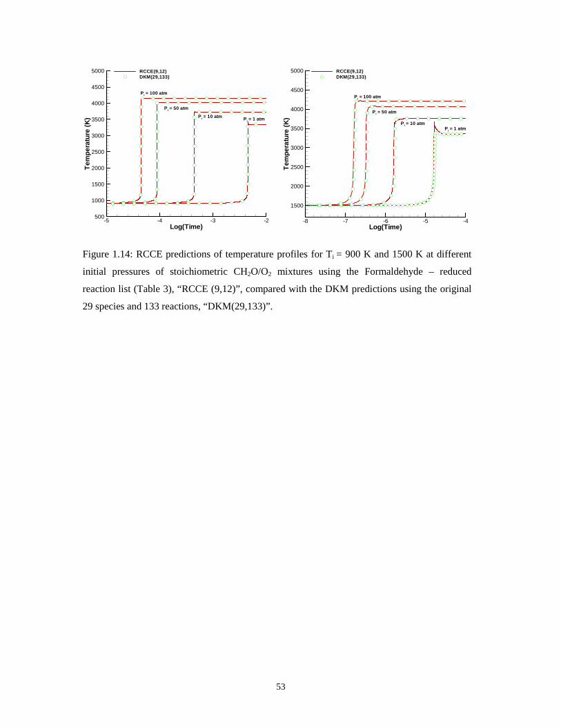
53
Log(Time)
Tem
per
atu
re(K
)
-5 -4 -3 -2500
1000
1500
2000
2500
3000
3500
4000
4500
5000 RCCE(9,12)DKM(29,133)
Pi = 1 atm
Pi = 100 atm
P i = 10 atm
P i = 50 atm
Log(Time)
Tem
per
atu
re(K
)
-8 -7 -6 -5 -4
1500
2000
2500
3000
3500
4000
4500
5000 RCCE(9,12)DKM(29,133)
Pi = 100 atm
Pi = 1 atmPi = 10 atm
Pi = 50 atm
Figure 1.14: RCCE predictions of temperature profiles for Ti = 900 K and 1500 K at different
initial pressures of stoichiometric CH2O/O2 mixtures using the Formaldehyde – reduced
reaction list (Table 3), “RCCE (9,12)”, compared with the DKM predictions using the original
29 species and 133 reactions, “DKM(29,133)”.

54
Chapter 2
Combustion Modelling of Methane-Air Mixtures Using the
Rate-Controlled Constrained-Equilibrium Method

55
Combustion Modelling of Methane/Air Mixtures Using the
Rate-Controlled Constrained-Equilibrium Method
G. Nicolas, M. Janbozorgi and H. Metghalchi1
Department of Mechanical and Industrial Engineering, Northeastern University, Boston,
MA 02115, USA
The method of Rate-Controlled Constrained-Equilibrium (RCCE) has been used
to study the ignition of methane/air mixtures. The method is based on local
maximization of entropy or minimization of a relevant free energy at any time
during the non-equilibrium evolution of the system subject to a set of kinetic
constraints. These constraints are imposed by slow rate-limiting reactions. Direct
integration of the rate equations for the constraint potentials has been used, once
the values of which are known, the concentration of all species can be calculated.
The RCCE calculations involve 16 total constraints and the results are in good
agreement with those obtained by direct integration of a full set of 60 species rate
equations over a wide range of temperatures and pressures. The reactor model is
constant volume and constant energy. Also, the recently suggested corrections of
Chaos and Dryer, Int. J. of Chem. Kin., 2010, 42: 143–150, have been made to
the reactor model and the predictions in ignition delay time have been compared
with the shock tube experimental data over initial pressures of 1atm-20atm and
initial temperatures of 900K -1500K.
2.1 Introduction
The development of kinetic models for describing the time evolution of chemically
reacting systems is a fundamental objective of chemical kinetics. Such models can easily
include several hundred of species and several thousands of reactions for heavy hydrocarbon
fuels. The fact that the equations governing the dynamics under such models are highly stiff
necessitates the development of tools to reduce the complexity of the model while

56
maintaining the degree of detail of predictions. Many approaches for this problem have been
proposed over the last two decades among which are the Quasi-Steady State Approximation
QSSA [1], Partial Equilibrium Approximation PEA [2], Intrinsic Low Dimensional
Manifolds (ILDM) [3], Computational Singular Perturbation [4], Adaptive Chemistry [5],
Directed Relation Graph (DRG) [6], ICE-PIC method [7], Slow Inertial Manifolds, SIM [15]
and Rate-Controlled Constrained-Equilibrium (RCCE) [8].
In this paper we use the method of RCCE to study the kinetics of Methane/Oxygen
under constant volume, constant energy constraints. The model includes the formation of C2
species from Methane and is in fact the extension of Janbozorgi et. al.’s model [11], in which
only C1 chemistry was considered.
Perhaps the most appealing feature of RCCE, as has also been explained in [11] is
that, contrary to all dimension reduction models in which the constrained equilibrium
assumption is not used, it is not necessary to start with a detailed kinetic model (DKM)
which must then be simplified by various mathematical approximations. Instead, one starts
with a small number of constraints, to which more constraints can be added, if necessary, to
improve the accuracy of the calculations. The number of constraints needed to describe the
dynamic state of the system within experimental accuracy can be very much smaller than the
number of species in the system. Therefore fewer reactions are needed to describe the
system’s evolution. Given the fact that in the entire body of thousands of chemical reactions
perhaps less than hundred have rate constants known better than a factor of two, this feature
of RCCE could help remove a great deal of uncertainty from the system by properly invoking
the constrained-equilibrium assumption. Reactions which do not change any constraint are in
constrained-equilibrium and need not to be specified. Nonetheless, the successful
implementation of the RCCE method depends critically on the choice of constraints and
knowledge of the rates of the constraints-changing reactions is required. Although several
important steps have been taken toward automatic selection of single species as constraints
[18-19], the work of Janbozorgi et. al. [11] shows that the optimum set of structural
constraints is still a research subject. The aim of this paper is to present a set of structural
constraints based on a careful study of the kinetics of the system, which yields good
agreements with the corresponding DKM over a wide range of initial temperatures, pressures

57
and equivalence ratios. Also, the ignition delay time predictions are compared with the RCM
and Shock Tube experimental data.
2.2 Rate-Controlled Constrained-Equilibrium
An excellent presentation of the theoretical foundations of RCCE can be found in [9].
Also, the working equations and initialization of the calculations are presented in [11, 16, and
17]. One major area of research in RCCE is selection of RCCE constraints. Constraints could
be either linear combinations of species or single species. Methodologies based on the greedy
algorithm [19] and index of importance, IOI, have been developed to select the single species
as constraints, although the greedy algorithm could in principle be used for group of species
as well. The algorithm presented in [17] and studies based on careful considerations of
chemistry [11] aim at determining the constrained-equilibrium paths, which may or may not
result in linear combination of species.
The main aim of our studies in RCCE is directed toward identifying the pattern of
conversion of heavy hydrocarbons to smaller ones and ultimately to combustion products.
Given the importance of the C1 chemistry in combustion of all heavy hydrocarbons, we
continue our efforts by building upon the C1 RCCE model developed in [11] to account for
C1/C2 interactions. The C1 mechanism is taken from [11], which includes the C1/H/O from
GRI-mech3.0 [10] plus additional peroxide species and reactions, enabling the model to be
used at high pressures and low temperatures. The C2 sub-mechanism is taken from GRI-
mech3.0. The constraints identified through studies of chemistry and also the RCCE reaction
flow diagrams are shown in table 2.1 and figure 2.1 respectively.
Table 2.1: C1/C2 constraints Constraint Definition of the constraint 1 EN Elemental Nitrogen 2 EC Elemental Carbon 3 EH Elemental Hydrogen 4 EO Elemental Oxygen 5 M Total number of moles 6 FV Moles of free valence(any unpaired valence electron) 7 FO Moles of free oxygen(any oxygen not directly attached to another oxygen) 8 FU Moles of fuel molecules 9 FR Moles of fuel radicals 10 DCO Moles of HCO+CO 11 OHO Moles of water radicals (OH+O) 12 APO Moles of alkyl peroxides(CH3OO+ CH3OOH+ CH2OOH) 13 ALCD Moles of alcohols + aldehydes(CH3O+CH3OH+CH2O+CH2OH) 14 C-C Moles of C-C Bond 15 C2H6 Moles of C2H6
16 C2H5 + C2H4 Moles of C2H5 + C2H4

58
The discussion pertinent to the first 13 constraints can be found in [11]. The extra three
constraints, namely C-C, C2H6 and C2H5+C2H4 were identified in this work. The aim has
been to identify a set which results in equally good agreements with the corresponding DKM
over a wide range of initial temperatures, pressures and equivalence ratios.
2.3 Results and discussions
Ignition of CH4/O2/N2 in an adiabatic constant volume reactor has been studied over a
wide range of initial temperatures (900K-1500K), initial pressures (1atm-20atm) and
stoichiometric ratios (0.6-1.2). The 16 constraints showed in able 2.1 were used in the RCCE
calculations. RCCE calculations were compared with those of DKM involving C1/C2
chemistry that includes 17 Nitrogen species and 43 C/H/O species.
2.3.1 C1/C2 oxidation
As stated earlier, discussions related to the first 13 constraints can be found in [11] in which
only C1 chemistry was considered. In the case of close to stoichiometric or rich conditions
the path from C1 to C2 becomes important, which introduces an important structural
constraint on the C-C bonds. A change in the value of this constraint is a necessary and
sufficient condition for formation or consumption of heavier hydrocarbons, in this case C2
and C3 species. The next constraint identified is C2H6, which in a species map is directly
connected to C2H5. The calculations of the rate of formation and consumption of C2H6
compared to the rate of consumption of C2H5 show that C2H6 is an important rate-controlling
constraint over a wide range of thermodynamic conditions. Such calculations further show
that the path from C2H5 to C2H4 can be assumed equilibrated subject to formation of C2H5
and consumption of C2H4, that is C2H5 + O � CH3 + CH2O and C2H4 + HO2 � C2H3 + H2O2
coupled with the constrained equilibrium reaction C2H5 + O2 � C2H5 + HO2 define C2H5 +
C2H4. This number of constraints is enough to put the predictions of RCCE within, in the
worst case, 5% of accuracy with respect to DKM. The model consistency demonstrates the
same level of agreement over the entire range of (φ,,Tp ). Illustrative results including

59
( φ,,Tp ) dependence studies are shown in figure 2.2. Also, concentrations are in good
agreement with their corresponding DKM.
2.3.2 Comparison with Shock Tube Data
As stated in the previous section, the predictions of the RCCE model consistently fall
within, in the worst case, 5% of the DKM predictions. In order to check whether this level of
accuracy is acceptable or not, comparisons were made against the experimental data of Shock
tube [14]. However, it is well known that making comparisons to Shock Tube data,
especially at low temperatures, requires modifications in the reactor model, since the constant
volume - constant energy model does not hold due to pressure changes during the delay time,
[12, and 13]. Two methods have been suggested for considering pressure corrections;
CHEMSHOCK [20] and the isentropic compression [21]. The isentropic assumption implies
non-reacting gas, while the delay time is certainly not isentropic. In this study we considered
a third possibility, i.e. the prescribed pressure, in which volume is obtained as part of the
solution of the reacting system, given the experimental pressure curve during the delay time
which is typically similar to figure 2.3. Dryer et al. [12] suggested a pressure profile
approximation as having a constant pressure for a finite amount of time and then increasing
linearly until the moment of ignition. Values of 1 – 5 ms and 1~10%/ms were considered for
the constant pressure duration and dP/dt respectively. Figure 2.4 demonstrates the results
before and after making the modification. Obviously, predictions show a consistent
improvement after implementing the correction. Since, in principle, predictions at high
enough temperatures were not expected to require modifications, it means that the DKM
model is not predictive at this range of temperature in the first place, although pressure
corrections make great improvements in the predictions of the model.
2.4 Summary and conclusions
RCCE calculations of CH4/O2/N2 have been made over a wide range of initial
temperatures, pressures and equivalence ratios using up to 16 constraints and 352 reactions

60
and good agreements with “Detailed kinetic Model” (DKM) calculations using 60 species
were obtained. The model RCCE demonstrates consistent accuracies, ranging from 0.05-
1.5%, with respect to the corresponding DKM. Such predictions are also in good agreement
with the Shock Tube data after considering the variable pressure effects in ignition delay
period.
Important features of RCCE are:
1. It is based on the well-established Maximum Entropy Principle of Thermodynamics rather
than mathematical approximations.
2. The total number of constraints required to determine the equilibrium state of a system can
be much smaller than the number of species in the system so fewer rate equations are
required to describe its evolution.
3. Every species for which the thermodynamic data is available can evolve dynamically
based on the constrained-equilibrium requirement. This feature could be used to investigate
whether a species, which is not explicitly included in the kinetic model, may be kinetically
important or not.
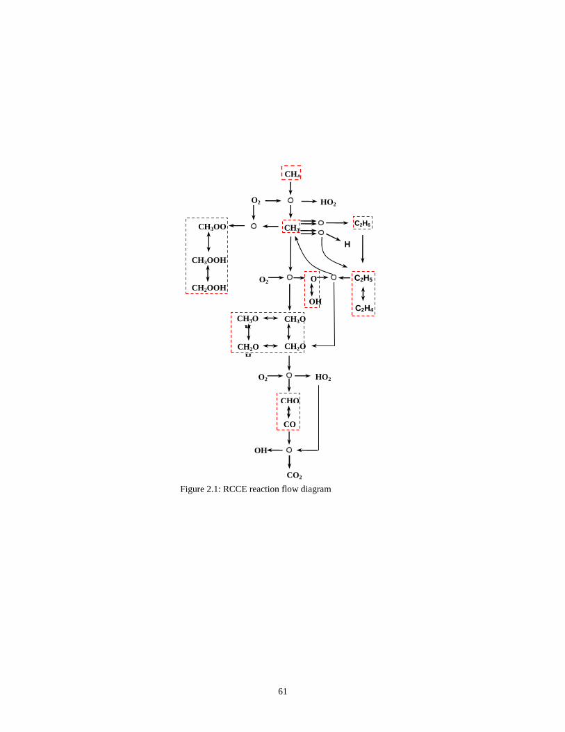
61
CH4
O2 HO2
CH3
O2
CH3OO
CH3OOH
CO
CH2OOH
O2
CHO
HO2
OH
CO2
C2H6
O
OH
C2H5
C2H4 CH3O CH3O
H
CH2OH
CH2O
H
Figure 2.1: RCCE reaction flow diagram

62
Log Time(sec)
Tem
per
atur
e(K
)
-5 -4 -3 -2 -1900
1200
1500
1800
2100
2400
2700
3000
DKM-Ti = 900KRCCE-Ti = 900KDKM-Ti = 1000KRCCE-Ti = 1000KDKM-Ti = 1100KRCCE-Ti = 1100KDKM-Ti = 1200KRCCE-Ti = 1200K
Phi = 0.8Pi = 20 atm
Log Time(sec)
Tem
pera
ture
(K)
-3 -2.5 -2 -1.5 -1 -0.5 0 0.5
1000
1500
2000
2500
3000
DKM- Pi = 1 atmDKM- Pi = 5 atmDKM- Pi = 10 atmDKM- Pi = 20 atmRCCE- Pi = 1 atmRCCE- Pi = 5 atmRCCE- Pi = 10 atmRCCE- Pi = 20 atm
Phi = 1.0Ti = 900 K
Log Time(sec)
Tem
pera
ture
(K)
-1.7 -1.6 -1.5 -1.4 -1.3 -1.2
1000
1200
1400
1600
1800
2000
2200
2400
2600
2800
3000
DKM- Phi =0.6RCCE - Phi =0.6DKM- Phi =1.0RCCE - Phi =1.0DKM - Phi=1.2RCCE - Phi =1.2
Ti = 900 KPi = 20 atm
Log Time(sec)
Log
Co
ncen
trat
ion
-4 -3 -2 -1-15
-12
-9
-6
-3
DKM-CH4RCCE-CH4DKM-O2RCCE-O2DKM-CO2RCCE-CO2DKM-CORCCE-CODKM-HO2RCCE-HO2DKM-H2ORCCE-H2O
Phi = 0.8Ti = 900 KPi = 20 atm
Frame 001 04 Feb 2011 Frame 001 04 Feb 2011
Log Time(sec)
Log
Con
cen
trat
ion
-4 -3 -2 -1-18
-15
-12
-9
-6DKM-HO2DKM-H2O2DKM-OHDKM-CH3DKM-CH3OOHDKM-CH3OORCCE-HO2RCCE-H2O2RCCE-OHRCCE-CH3RCCE-CH3OOHRCCE-CH3OO
Phi = 0.8Ti = 900 KP = 20 atm
Log Time(sec)
Log
Con
cen
trat
ion
-6 -5 -4 -3 -2 -1-21
-18
-15
-12
-9
-6
DKM-CH3RCCE-CH3DKM-C2H6RCCE-C2H6DKM-C2H4RCCE-C2H4
Phi = 0.8Ti = 900 KPi = 20 atm
Figure 2.2. (a) Ti-dependence, (b) Pi-dependence and (c) φ - dependence studies, (d,e,f) species concentrations
(a) (b)
(c) (d)
(e) (f)

63
10
100
1000
10000
4.75 5 5.25 5.5 5.75 6 6.25 6.5 6.75 7 7.25
10000/T
Ign
itio
n D
elay
Tim
e(µ
s)
RCCEDKMPres. FitPetersen
Figure 2.3: Pressure profile approximation from Chaos and Dryer [12]
Figure 2.4: Comparison in ignition delay time after using the prescribed pressure. Experimental data from Petersen et al. [14]
2.5 References
[1] S.W. Benson, J.Chem. Phys. 20 (1952) 1605.
[2] M. Rein, Phys.Fluids A 4 (1992) 873.
[3] U. Maas, S.B. Pope, Combust. Flame 88 (1992) 239.
[4] S.H. Lam, D.A. Goussis, Proc. Combust. Inst. 22 (1988) 931.
[5] O. Oluwole, B. Bhattacharjee, J.E. Tolsma, W.H. Green, Combust. Flame 146 (1-2) (2006)
348-365.
[6] T. Lu, C.K. Law, Combust. Flame 144(1-2) (2006) 24-36.
[7] Z. Ren, S.B. Pope, A. Vladimirsky, J.M. Guckenheimer, The ICE-PIC method for the
dimension reduction of chemical kinetics, Chem. Phys. 124 (114111) (2006).
[8] J.C. Keck and D. Gillepsie, Combust. Flame 17 (1971) 237.
[9] J.C. Keck, Prog. Energy Combust. Sci. 16 (1990) 125.
[10]http://www.me.berkeley.edu/gri-mech/version30/text30.html.
[11] M. Janbozorgi, S. Ugarte, M. Metghalchi, J.C. Keck, Combust. Flame 156 (2009) 1871-
1885.
[12] M. Chaos, F. Dryer, Int. J. of Chem. Kin., 2010, 42: 143–150
[13] D.F. Davidson, R.K. Hanson, Int. J. of chemical kinetics 36, 510-523 (2004).
[14] E.L. Petersen, J.M. Hall, S.D. Smith, J. de Vries, A.R. Amadio, and M.W. Crofton, Journal
of Engineering for Gas Turbines and Power, Vol. 129, 2007, pp. 937-944.

64
[15] Ashraf N. Al-Khateeb, Joseph M. Powers, Samuel Paolucci, Andrew J. Sommese, Jeffrey
A. Diller, Jonathan D. Hauenstein, and Joshua D. Mengers, J. Chem. Phys. 131, 024118 (2009).
[16] V.A. Yousefian, Rate-controlled constrained-equilibrium thermo chemistry algorithm
for complex reacting systems, Combust. Flame 115 (1998) 66–80.
[17] W.P. Jones, S. Rigopoulos, Rate-controlled constrained equilibrium: formulation and
application of non-premixed laminar flames, Combust. Flame 142 (2005) 223–234.
[18] Q. Tang and S.B. Pope, Combustion Theory and Modeling, (2004), 8, 255--279.
[19] V. Hiremath, Z. Ren, S. B. Pope, A Greedy Algorithm for Species Selection in
Dimension Reduction of Combustion Chemistry, Combustion Theory and Modelling,
December 2009, 1–27
[20] H. Li, Z.C. Owens, D.F. Davidson and R.K. Hanson, Int. J. of Chemical Kinetics 40,
189-198 (2008)
[21] Fieweger, K.; Blumenthal, R.; Adomeit, G. Combust. Flame 1997, 109, 599–619.

65
Chapter 3
Rate-Controlled Constrained-Equilibrium Theory Appl ied to Expansion of Combustion Products in the Power Stroke of an Internal Combustion Engine
Mohammad Janbozorgi and Hameed Metghalchi
Department of Mechanical and Industrial Engineering, Northeastern University, Boston, Massachusetts 02115-5000, USA
Published in Int. J. of Thermodynamics - Vol. 12 (No. 1), pp. 44-50, March 2009

66
Rate-Controlled Constrained-Equilibrium Theory Appl ied to Expansion of Combustion Products in the Power Stroke of an Internal Combustion
Engine
Mohammad Janbozorgi and Hameed Metghalchi ([email protected])
Department of Mechanical and Industrial Engineering, Northeastern University, Boston, Massachusetts 02115-5000, USA
Rate-controlled constrained-equilibrium method, firmly based on the second law of thermodynamics, is applied to the expansion of combustion products of methane during the power stroke of an internal combustion engine. The constraints used in this study are the elemental oxygen, hydrogen, carbon and nitrogen together with other four dynamic constraints of total number of moles, moles of DCO (CO+HCO), moles of free valence and moles of free oxygen. Since at chemical equilibrium, the mixture composition is dominated by H/O, CO/CO2, and a few other carbon-containing species, almost independent of the fuel molecule, the set results in accurate predictions of the kinetic effects observed in all H/O and CO/CO2 compounds and temperature history. It is shown that the constrained-equilibrium predictions of all the species composed of the specified atomic elements can be obtained independent of a kinetic path, provided their Gibbs free energies are known.
Keywords: Second law of thermodynamics, The Rate-controlled constrained-Equilibrium (RCCE) method, Constraints, Chemical kinetics, Internal combustion engine, Power stroke.
3.1 Introduction
Equilibrium gas dynamics is based on the assumption that when a system undergoes an either heat or work interaction with the surrounding environment, the internal molecular relaxation processes are faster than changes brought about in system’s thermodynamic states due to interaction. Under this assumption the condition of local thermodynamic equilibrium (LTE) is valid. LTE leads to thermal equilibrium among various molecular degrees of freedom, enabling the definition of a single temperature. However, this is not generally the case, as energy re-distribution among internal degrees of freedom (translation, rotation, vibration, and electronics) requires definite lengths of time, known as relaxation times (Vincenti, Kruger, 1965). If the interaction occurs on a time scale shorter or comparable with molecular relaxation, the internal dynamics of the system lags behind in re-establishing local thermodynamic equilibrium and the slow degree of freedom has to be treated by means of non-equilibrium thermodynamics.
This study is focused on gas phase chemical relaxation, where a chemically reacting system undergoes work interaction with the environment and is initially in a chemical equilibrium state. As pointed out by Keck (1990), an equilibrium state is meaningful only when the constraints, subject to which such a state is attained, are carefully determined and all equilibrium states are in fact constrained equilibrium states. At temperatures of interest to combustion, nuclear and ionization reactions can be assumed frozen and the fundamental constraints imposed on the system are conservation of neutral atoms. The cascade of
67
constraints can be easily extended based on the existence of classes of slow chemical or energy-exchange reactions, which if completely inhibited would prevent the relaxation of the system to complete equilibrium. For instance, total number of moles in a reacting system does not change unless a three body reaction occurs, radicals are not generated in the absence of chain branching reactions and the definition of a single temperature in a chemically reacting system is based on the observation that thermal equilibration among translation, rotation and vibration is in general faster than chemical reactions.
Based on the most profound law of nature, i.e. second law of thermodynamics, Rate-Controlled Constrained-Equilibrium (RCCE) method was originally developed by Keck and Gillespie (1971) and later by Keck and coworkers (Bishnu, Hamiroune, Metghalchi, Keck, 1997 and Hamiroune, Bishnu, Metghalchi, Keck, 1998), Tang and Pope (2004) and Jones and Rigopoulos (2005) to estimate the state of a nonequilibrium system by maximizing entropy at any time during the nonequilibrium evolution subject to the known constraints imposed on the system. The dynamics of the unrepresented part of the system is then determined by the requirement of constrained equilibrium.
According to the fundamental premise of RCCE, slow reactions in a complex reacting system impose constraints on its composition, which control the rate at which it relaxes to chemical equilibrium, while the fast reactions equilibrate the system subject to the constraints imposed by the slow reactions. Consequently, the system relaxes to chemical equilibrium through a sequence of constrained-equilibrium states at a rate controlled by the slowly changing constraints (Keck, 1990).
Morr and Heywood (1974) considered the problem of sudden cooling of the combustion products of aviation kerosene, by passing the combustion products through an energy exchanger at constant pressure as a model for gas turbine. They compiled a model for CO oxidation chemistry based on the fact that three body and CO oxidizing reactions are generally slower than other reactions and confirmed the notion through comparison against experimental data. In this paper we look at the expansion of (CH4/O2/N2) combustion products in the power stroke of an internal combustion engine, when N2 is assumed to be inert, using the RCCE method. This method enables a systematic analysis of the underlying kinetics through testing different constraints with the least amount of effort.
3.2 Physical Model
The physical model is shown in figure 3.1. It is assumed that power stroke begins with the combustion products at a complete chemical equilibrium state and that expansion occurs so rapidly that heat conduction does not occur through the piston wall. It is further assumed that the gas composition is homogeneous at any time during expansion. Volume is assumed to be a prescribed function of time (Heywood, 1988):
)()1(2
11
)( θfrV
tVc
c
×−+= , (3.1)
where
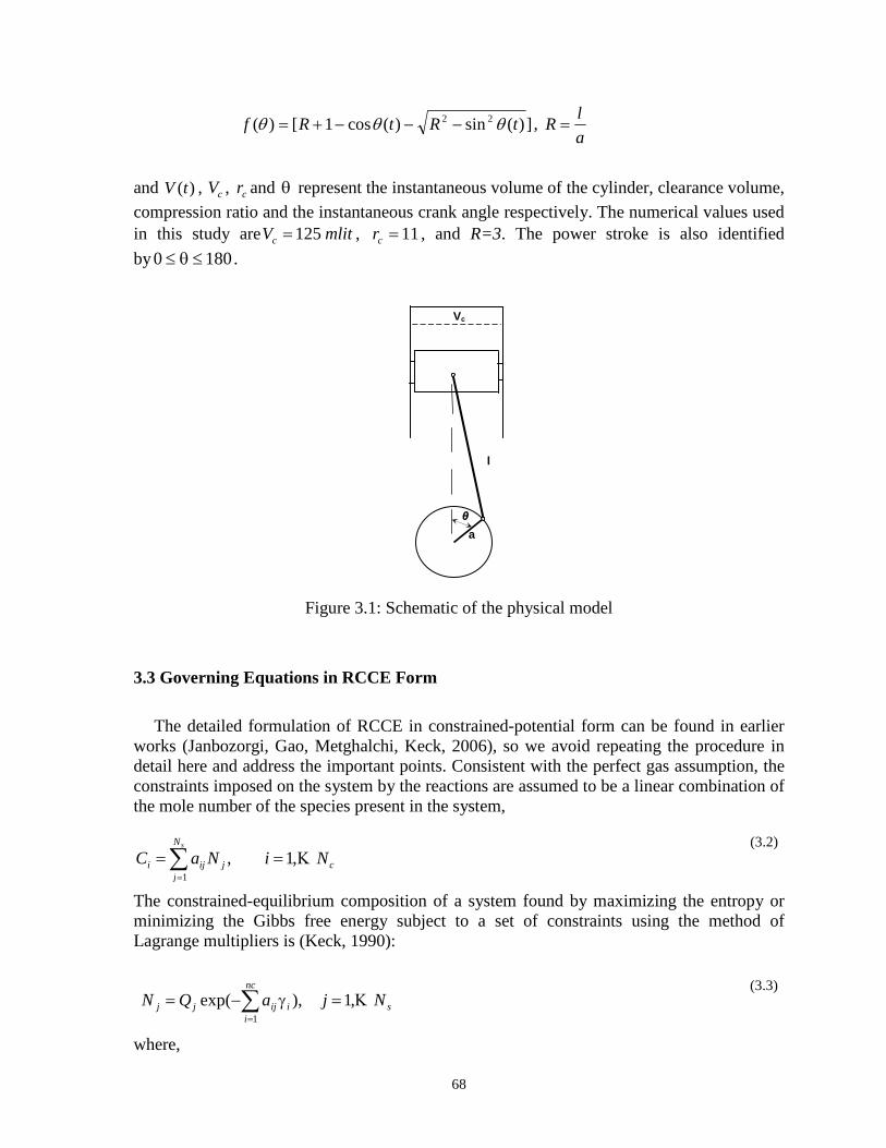
68
])(sin)(cos1[)( 22 tRtRf θθθ −−−+= , a
lR=
and )(tV , cV , cr and θ represent the instantaneous volume of the cylinder, clearance volume,
compression ratio and the instantaneous crank angle respectively. The numerical values used in this study are mlitVc 125= , 11=cr , and R=3. The power stroke is also identified
by 1800 ≤θ≤ .
Figure 3.1: Schematic of the physical model
3.3 Governing Equations in RCCE Form
The detailed formulation of RCCE in constrained-potential form can be found in earlier works (Janbozorgi, Gao, Metghalchi, Keck, 2006), so we avoid repeating the procedure in detail here and address the important points. Consistent with the perfect gas assumption, the constraints imposed on the system by the reactions are assumed to be a linear combination of the mole number of the species present in the system,
cj
N
jiji NiNaC
s
Κ,1,1
==∑=
(3.2)
The constrained-equilibrium composition of a system found by maximizing the entropy or minimizing the Gibbs free energy subject to a set of constraints using the method of Lagrange multipliers is (Keck, 1990):
s
nc
iiijjj NjaQN Κ,1),exp(
1
=γ−= ∑=
(3.3)
where,
a
l
Vc
θ

69
)exp( 0jj RT
VpQ µ−= ο
(3.3a)
Clearly, the partition function of each species depends on temperature, volume and the standard Gibbs free energy of the species. The time rate of change of constraints or equivalently, constraint potentials, can be obtained by taking the time derivative of equation (3.2) as:
j
N
jiji NaC
s
&& ∑=
=1
(3.4)
It is assumed that changes in the chemical composition are the results of chemical reactions of the form
r
N
jjjk
N
jjjk NkXX
ss
,,1,11
Κ=ν↔ν ∑∑=
+
=
− (3.5)
The phenomenological expression of chemical kinetics can be used to replace jN& in
equation (3.4)
k
N
kjkj rN
r
∑=
ν=1
& (3.6)
where
−+ −= kkk rrr (3.6a)
+− ν−ν=νjkjkjk (3.6b)
Substituting equation (3.6) into (3.4) results in the required time rate of change of the constraint Ci:
∑=
=rN
kkiki rbC
1
& (3.7)
∑=
ν=sN
jjkijik ab
1
(3.7a)
Clearly, a reaction k for which the value of bik is zero for all constraints i is in constrained equilibrium. All reactions in the mechanism must satisfy this condition for elemental constraints. In the absence of any spatial nonhomogeneity, the implicit differential equations governing the constraint potentials can be obtained by substituting equation (3.7) and the time derivative of equation (3.3) into equation (3.4), the final result of which is:
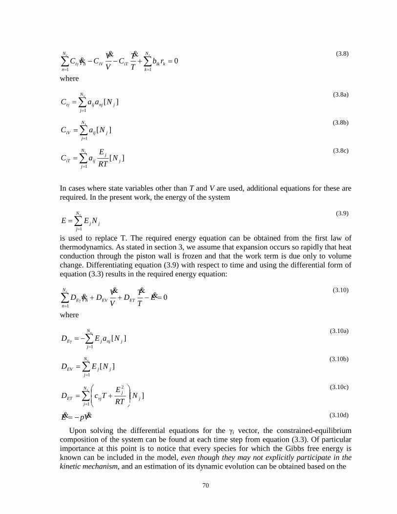
70
011
=+−−γ ∑∑==
γ k
N
kikiTiVn
N
ni rb
T
TC
V
VCC
rc &&&
(3.8)
where
][1
jnj
N
jiji NaaC
s
∑=
γ = (3.8a)
][1
j
N
jijiV NaC
s
∑=
= (3.8b)
][1
jj
N
jijiT N
RT
EaC
s
∑=
= (3.8c)
In cases where state variables other than T and V are used, additional equations for these are required. In the present work, the energy of the system
∑=
=sN
jjj NEE
1
(3.9)
is used to replace T. The required energy equation can be obtained from the first law of thermodynamics. As stated in section 3, we assume that expansion occurs so rapidly that heat conduction through the piston wall is frozen and that the work term is due only to volume change. Differentiating equation (3.9) with respect to time and using the differential form of equation (3.3) results in the required energy equation:
01
=−++γ∑=
γ ET
TD
V
VDD ETEVn
N
nE
c
&&&
& (3.10)
where
][1
jnj
N
jjE NaED
s
∑=
γ −= (3.10a)
][1
j
N
jjEV NED
s
∑=
= (3.10b)
][1
2
j
N
j
jvjET N
RT
ETcD
s
∑=
+=
(3.10c)
VpE && −= (3.10d)
Upon solving the differential equations for the γi vector, the constrained-equilibrium composition of the system can be found at each time step from equation (3.3). Of particular importance at this point is to notice that every species for which the Gibbs free energy is known can be included in the model, even though they may not explicitly participate in the kinetic mechanism, and an estimation of its dynamic evolution can be obtained based on the

71
value of the known constraints. Such dynamic evolution is dictated by the requirement of constrained-equilibrium. In the limit of local chemical equilibrium, where all reactions are in constrained-equilibrium, the constraints imposed by the conservation of neutral atoms enables determining the concentration of every possible species made up of the same elements. Such an approach is the basis of the widely used STANJAN and NASA equilibrium codes (Reynolds, Gordon, McBride, 1971). Evidently, different sets of constraints can be handled with the same ease using the above formulations.
3.4 Constraints
The selection of appropriate constraints is the key to the successful application of the RCCE method. Among the general requirements for the constraints are that they must (1) be linearly independent combinations of the species mole numbers, (2) include the elements, (3) determine the energy and entropy of the system within experimental accuracy, and (4) hold the system in the specified initial state. In addition, they should reflect whatever information is available about rate-limiting reactions controlling the time evolution of the system. The constraints used in this study are listed in Table 3.1.
According to the Le Châtelier principle, when a highly dissociated mixture undergoes an interaction with the environment which lowers the gas temperature and density, the internal dynamics shift in the exothermic direction to minimize the cooling effect of interaction. As a result, three body recombination reactions become an important part of the energy restoration process. The total number of particles in the system does not change unless one such reaction occurs. This is the rationale for putting a constraint on total number of moles; M. Among the reactions changing this constraint is: H+H+M=H2+M O+H+M=OH+M O+O+M=O2+M H+OH+M=H2O+M Oxidation of CO to CO2 constitutes an important part of the exothermic relaxation which is dominated by several reactions, such as: HCO+X = CO+HX, X = radical pool (R3)
HCO+O2=CO+HO2 (R2)
CO+OH = CO2+H (R3)
-25
-20
-15
-10
-5
0
N2
H2O
CO
2
CO
O2
OH
H2
H
O
HO
2
H2O
2
HO
CO
HC
O
HO
CH
O
CH
2O
CH
2OH
CH
3
CH
2
C
CH
4
CH
CH
3OH
CH
3O
HO
OC
O
OC
HO
CH
3OO
CH
3OO
H
CH
2OO
H
OO
CH
O
HO
OC
HO
Lo
g(M
ole
Fra
ctio
n)
Figure 3.2: Chemical equilibrium composition of stoichiometric CH4/O2/N2 mixture.
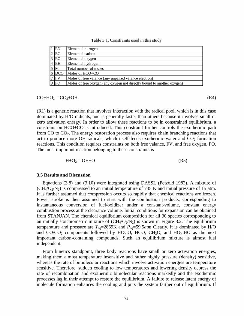
72
CO+HO2 = CO2+OH (R4)
(R1) is a generic reaction that involves interaction with the radical pool, which is in this case dominated by H/O radicals, and is generally faster than others because it involves small or zero activation energy. In order to allow these reactions to be in constrained equilibrium, a constraint on HCO+CO is introduced. This constraint further controls the exothermic path from CO to CO2. The energy restoration process also requires chain branching reactions that act to produce more OH radicals, which itself feeds exothermic water and CO2 formation reactions. This condition requires constraints on both free valance, FV, and free oxygen, FO. The most important reaction belonging to these constraints is
H+O2 = OH+O (R5)
3.5 Results and Discussion
Equations (3.8) and (3.10) were integrated using DASSL (Petzold 1982). A mixture of (CH4/O2/N2) is compressed to an initial temperature of 735 K and initial pressure of 15 atm. It is further assumed that compression occurs so rapidly that chemical reactions are frozen. Power stroke is then assumed to start with the combustion products, corresponding to instantaneous conversion of fuel/oxidizer under a constant-volume, constant energy combustion process at the clearance volume. Initial conditions for expansion can be obtained from STANJAN. The chemical equilibrium composition for all 30 species corresponding to an initially stoichiometric mixture of (CH4/O2/N2) is shown in Figure 3.2. The equilibrium temperature and pressure are Teq=2869K and Peq=59.5atm Clearly, it is dominated by H/O and CO/CO2 components followed by HOCO, HCO, CH2O, and HOCHO as the next important carbon-containing compounds. Such an equilibrium mixture is almost fuel independent.
From kinetics standpoint, three body reactions have small or zero activation energies, making them almost temperature insensitive and rather highly pressure (density) sensitive, whereas the rate of bimolecular reactions which involve activation energies are temperature sensitive. Therefore, sudden cooling to low temperatures and lowering density depress the rate of recombination and exothermic bimolecular reactions markedly and the exothermic processes lag in their attempt to restore the equilibrium. A failure to release latent energy of molecule formation enhances the cooling and puts the system farther out of equilibrium. If
Table 3.1. Constraints used in this study
1 EN Elemental nitrogen2 EC Elemental carbon3 EO Elemental oxygen4 EH Elemental hydrogen5 M Total number of moles6 DCO Moles of HCO+CO7 FV Moles of free valence (any unpaired valence electron)8 FO Moles of free oxygen (any oxygen not directly bound to another oxygen)
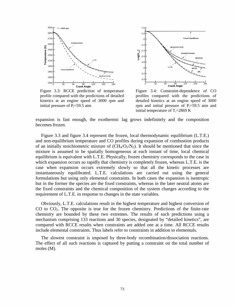
73
expansion is fast enough, the exothermic lag grows indefinitely and the composition becomes frozen.
Figure 3.3 and figure 3.4 represent the frozen, local thermodynamic equilibrium (L.T.E.)
and non-equilibrium temperature and CO profiles during expansion of combustion products of an initially stoichiometric mixture of (CH4/O2/N2). It should be mentioned that since the mixture is assumed to be spatially homogeneous at each instant of time, local chemical equilibrium is equivalent with L.T.E. Physically, frozen chemistry corresponds to the case in which expansion occurs so rapidly that chemistry is completely frozen, whereas L.T.E. is the case when expansion occurs extremely slowly so that all the kinetic processes are instantaneously equilibrated. L.T.E. calculations are carried out using the general formulations but using only elemental constraints. In both cases the expansion is isentropic but in the former the species are the fixed constraints, whereas in the later neutral atoms are the fixed constraints and the chemical composition of the system changes according to the requirement of L.T.E. in response to changes in the state variables.
Obviously, L.T.E. calculations result in the highest temperature and highest conversion of CO to CO2. The opposite is true for the frozen chemistry. Predictions of the finite-rate chemistry are bounded by these two extremes. The results of such predictions using a mechanism comprising 133 reactions and 30 species, designated by “detailed kinetics”, are compared with RCCE results when constraints are added one at a time. All RCCE results include elemental constraints. Thus labels refer to constraints in addition to elementals.
The slowest constraint is imposed by three-body recombination/dissociation reactions. The effect of all such reactions is captured by putting a constraint on the total number of moles (M).
Crank Angle
Tem
pera
ture
(K)
0 30 60 90 120 150 1801500
1650
1800
1950
2100
2250
2400
2550
2700
2850
3000
L.T.E.
Frozen Equilibrium
(M,DCO,FV,FO)
Detailed Kinetics
ω = 3000 rpm
Crank Angle
Log
(XC
O)
0 30 60 90 120 150 180
-3.4
-3.2
-3
-2.8
-2.6
-2.4
-2.2
-2
-1.8
-1.6
Frozen Equilibrium
(M,DCO)
L.T.E.(DCO)
(M,DCO,FV,FO)
(M)
Detailed Kinetics
Figure 3.3: RCCE prediction of temperature profile compared with the predictions of detailed kinetics at an engine speed of 3000 rpm and initial pressure of Pi=59.5 atm
Figure 3.4: Constraint-dependence of CO profiles compared with the predictions of detailed kinetics at an engine speed of 3000 rpm and initial pressure of Pi=59.5 atm and initial temperature of Ti=2869 K

74
Crank Angle
Tem
pera
ture
(K)
0 30 60 90 120 150 1801500
1650
1800
1950
2100
2250
2400
2550
2700
2850
3000 ω = 3000 rpm, 6000 rpm, 12000 rpm
(M,DCO,FV,FO)
L.T.E
Detailed Kinetics
Crank Angle
Log(
XC
O)
0 30 60 90 120 150 180-3.5
-3
-2.5
-2
-1.5 L.T.ERCCE (M,DCO,FV,FO)Detailed Kinetics
ω = 6000 rpm
ω = 3000 rpm
ω = 12000 rpm
φ =1
Figure 3.5: Engine-speed dependence of temperature profiles compared with the predictions of detailed kinetics at the equivalence ratio of 1.0
Figure 3.6: Engine-speed dependence of CO profiles compared with the predictions of detailed kinetics at the equivalence ratio of 1.0
Crank Angle
Tem
per
atu
re(K
)
Pre
ssu
re(b
ar)
0 30 60 90 120 150 1801400
1600
1800
2000
2200
2400
2600
2800
0
10
20
30
40
50
60
L.T.E.
Detailed Kinetics
(M,DCO,FV,FO)
φ = 0.8
Frozen Equilibrium
Pressure(detailed Kinetics)
Crank Angle
Log(
XC
O)
0 30 60 90 120 150 180-6
-5.5
-5
-4.5
-4
-3.5
-3
-2.5
-2
(M,DCO)
(M,DCO,FV,FO)
(M)
L.T.E.
Frozen Equilibrium
Detailed Kinetics
Figure 3.7: Temperature and pressure profiles under different conditions at an engine speed of 3000 rpm, initial temperature of Ti=2673 K, initial pressure of Ti=54.83 atm and equivalence ratio of 0.8
Figure 3.8: CO profiles under different sets of constraints at an engine speed of 3000 rpm, initial temperature of Ti=2673 K, initial pressure of Ti=54.83 atm and equivalence ratio of 0.8

75
Crank Angle
Tem
pera
ture
(K)
0 30 60 90 120 150 180
1600
1800
2000
2200
2400
2600
2800Frozen EquilibriumRCCE (M,DCO,FV,FO)Detailed KineticsL.T.E.
Crank Angle
Log
(XC
O)
0 30 60 90 120 150 180
-1.41
-1.395
-1.38
-1.365
-1.35
-1.335
-1.32
-1.305
-1.29
Frozen Equilibrium
(M,DCO,FV,FO)
L.T.E.
Detailed Kinetics
(DCO,FV)
RCCE (M)
(DCO)
Figure 3.9: Temperature profiles under different sets of constraints at an engine speed of 3000 rpm, initial temperature of Ti=2846.8 K, initial pressure of Ti=60.5 atm and equivalence ratio of 1.2
Figure 3.10: CO profiles under different sets of constraints at an engine speed of 3000 rpm, initial temperature of Ti=2846.8 K, initial pressure of Ti=60.5 atm and equivalence ratio of 1.2
Evidently adding to the list a constraint on DCO=HCO+CO does not change the predictions noticeably, meaning that these reactions (reactions similar to R3 and R4) are nearly in constrained equilibrium. However, the collective effect of DCO, FV, and FO results in perfect match between RCCE using 8 constraints and detailed kinetics using 30 species.
It is also interesting to notice that the state of the gas follows exactly the predictions of L.T.E. during the early stage of expansion, when the piston speed is very slow. Departures from local thermodynamic equilibrium emerge as the piston speed increases.
In order to check the validity of the identified constraints under faster expansions, engine
speed is increased to 6000 rpm and 12000 rpm. In this case the kinetic effects are only observed in species profiles and not in temperature. Figures 3.5 and 3.6 demonstrate these observations. Figures 3.7 and 3.8 show the same set of results for expansion of combustion products of a mixture of (CH4/O2/N2) with an initial equivalence ratio of 0.8. Progressive improvements of the results by adding constraints one at a time is evident. Pressure at the end of the stroke is 3 atm. Figures 3.9 and 3.10 show the same result for the case in which the initial equivalence ratio is 1.2. Contrary to the results corresponding to a stoichiometric mixture, Figure 3.4, in this case three body reactions are in constrained equilibrium and DCO-changing reactions are rate limiting.
Figure 3.11(a,b,c,d) represents the profiles of H2O, CO2, H, O, HO2, H2O2, HOCO, HCO,
HOCHO, CH2O, CO, O2, H2, OH corresponding to an equivalence ratio of 1.0 at an engine speed of 3000 rpm. Comparison has been made between RCCE calculations using 8 constraints against detailed kinetics using 30 species and 133 reactions. It should be noticed that HOCHO, CH2O and HOCO are not directly constrained and their evolution is determined based on the requirement of constrained equilibrium. This demonstrates one of the most important features of RCCE that with a few constraints the concentrations of all possible species composed of the specified elements can be readily obtained, provided their Gibbs free energies are known. Having defined the constraint DCO=HCO+CO, the

76
concentration of HCO is also determined based on an internal equilibrium with CO. Clearly, the single constraint DCO is able to give quite acceptable predictions for CO, figure 3.11d and HCO, figure 3.11c, which confirms the partial equilibrium between them.
3.6 Concluding Remarks
Local thermodynamic equilibrium (L.T.E.), frozen chemistry, detailed kinetics and Rate-
controlled constrained-equilibrium calculations of the expansion of (CH4/O2/N2) combustion products during the power stroke of an internal combustion engine were conducted. Looking at the dynamic of the expansion process, a set of 8 generalized constraints was identified. The set gives perfect matches with the results of detailed kinetics. The constraints identified are quite general and are able to handle relaxation from an initial equilibrium state of the combustion product of any hydrocarbon fuels. Under stoichiometric conditions, DCO-changing reactions are in constrained equilibrium and M-changing reactions are rate limiting, whereas, making the mixture richer, puts M-changing reactions in equilibrium and DCO-changing reactions out of equilibrium.
Of the salient features of the RCCE technique is that it is based on the most profound law of thermodynamics, Maximum Entropy Principle. Every species made up of the specified elements can be included in the model, provided its Gibbs free energy is known. In the absence of any direct constraint on a species or group of species, they will evolve according to the requirement of constrained-equilibrium. RCCE has the dazzling ability to carry out local thermodynamic equilibrium, frozen equilibrium and rate-controlled constrained-equilibrium calculations with the same ease, by implementing different classes of constraints. In the limit where the number of constraints equals the number of species, the method becomes exact.
Acknowledgments This work has been partially supported by the generous support of Army Research Office (ARO) corresponding to Grant No. W911NF0510051 under supervision of Dr. Ralph Anthenien, ARO
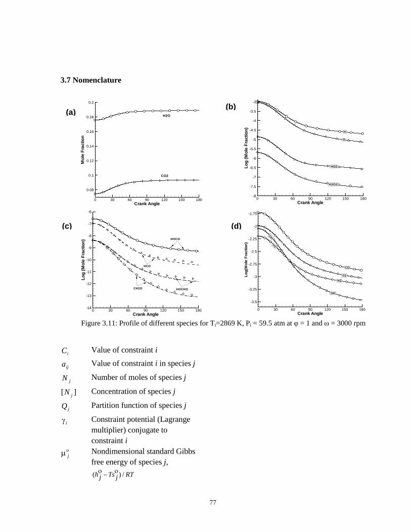
77
3.7 Nomenclature
iC Value of constraint i
ija Value of constraint i in species j
jN Number of moles of species j
][ jN Concentration of species j
jQ Partition function of species j
iγ Constraint potential (Lagrange multiplier) conjugate to constraint i
οjµ Nondimensional standard Gibbs
free energy of species j,
RTjTsjh /)( οο −
Crank Angle
Mol
eF
ract
ion
0 30 60 90 120 150 180
0.08
0.1
0.12
0.14
0.16
0.18
0.2
H2O
CO2
Crank Angle
Log
(Mol
eF
ract
ion)
0 30 60 90 120 150 180-8
-7.5
-7
-6.5
-6
-5.5
-5
-4.5
-4
-3.5
-3
H2O2
H
O
HO2
Crank Angle
Log
(Mol
eF
ract
ion)
0 30 60 90 120 150 180-14
-13
-12
-11
-10
-9
-8
-7
-6
CH2O
HOCO
HCO
HOCHO
Crank Angle
Log(
Mol
eF
ract
ion)
0 30 60 90 120 150 180
-3.5
-3.25
-3
-2.75
-2.5
-2.25
-2
-1.75
H2
CO
O2
OH
OH
H2
Figure 3.11: Profile of different species for Ti=2869 K, Pi = 59.5 atm at φ = 1 and ω = 3000 rpm
(a) (b)
(c) (d)

78
jE Molar energy of species j
ikb Change in constraint i by reaction k
kr Net rate of reaction k +
kr Forward rate of reaction k
−kr Reverse rate of reaction k
+νij Stoichiometric coefficient of product species j in reaction i
−νij Stoichiometric coefficient of reactant species j in reaction i
sN Number of species
cN Number of constraints
rN Number of reactions
vjc Frozen molar heat capacity of species j at constant volume
T Temperature V Volume p Pressure
οp Standard (atmospheric) pressure
E Total energy R Universal gas constant
5.3 References
Bishnu, P., Hamiroune, D., Metghalchi, M., and Keck, J.C., 1997, “Constrained-Equilibrium Calculations for Chemical Systems Subject to Generalized Linear Constraints using the NASA and STANJAN Equilibrium Program”, Combustion Theory and Modeling, Vol. 1, pp. 295-312.
Gordon, S. and McBride, B. J., 1971, NASA SP-273.
Heywood J. B. “ Internal Combustion Engine Fundamentals”, McGraw Hill Book Company, 1988.
Hamiroune, D., Bishnu, P., Metghalchi, M. and Keck, J.C., 1998, “Controlled Constrained Equilibrium Method using Constraint Potentials”, Combustion Theory and Modeling, Vol. 2, pp. 81.

79
Janbozorgi, M, Gao, Y., Metghalchi, H., Keck, J. C., 2006, “Rate-Controlled Constrained-Equilibrium Calculations of Ethanol-Oxygen Ignition Delay Times”, Proc. ASME (Int.), November 5-10, Chicago.
Jones, W. P., Rigopoulos, S., 2005, “Rate- Controlled Constrained-Equilibrium: Formulation and Application of Nonpremixed Laminar Flames”, Combust. Flame, Vol. 142 pp. 223– 234.
Keck, J. C., 1990, “Rate-Controlled Constrained-Equilibrium Theory of Chemical Reactions in Complex Systems”, Prog. Energy Combust. Sci., Vol. 16 pp. 125.
Keck, J. C., Gillespie, D., 1971, “Rate-Controlled Partial-Equilibrium Method for Treating Reacting Gas Mixtures”, Combustion and Flame Vol. 17, pp. 237. Morr, A. R., Heywood, J. B., 1974, Acta Astronautica, Vol. 1, pp. 949-966.
Petzold, L., 1982, “Differential-Algebraic Equations Are Not ODE’s”, SIAM J., Sci. Stat. Comput. Vol. 3, pp. 367.
Reynolds, W. C., STANJAN Program, Stanford University, ME270, HO#7
Tang, Q., Pope, S. B., 2004, “A More Accurate Projection in the Rate Controlled Constrained Equilibrium Method for Dimension Reduction of Combustion Chemistry”, Combustion Theory and Modeling, Vol., 8 pp. 255 - 279.
Vincenti, W. G., Kruger, C. H., 1965, Introduction to Physical Gas Dynamics, Krieger Publishing Company.

80
Chapter 4
Rate-Controlled Constrained-Equilibrium Modelling of Expansion of Combustion Products in a Supersonic Nozzle
Mohammad Janbozorgi and Hameed Metghalchi ([email protected])
Department of Mechanical and Industrial Engineering, Northeastern University, Boston,
2011 7th US National Combustion Meeting Organized by the Eastern States Section of the Combustion Institute
and Hosted by the Georgia Institute of Technology, Atlanta, GA March 20-23, 2011

81
4.1 Introduction Under a broad range of conditions encountered in chemical nozzles, departures
from Boltzmann distribution among private molecular degrees of freedom can be
neglected. Under this condition the gas can be assumed in thermal equilibrium, which
enables definition of a single temperature and, therefore, the only major non-equilibrium
phenomenon is associated with chemical reactions. This part of research was focused on
the gas phase chemical relaxation in a supersonic diverging nozzle using the RCCE
method. The system is considered to be initially at equilibrium at a Mach number of 1.0,
which subsequently expands to lower densities and higher Mach numbers. Depending on
how fast the expansion occurs the system could relax through a series of shifting
chemical equilibrium, chemical non-equilibrium or frozen chemical equilibrium states,
each of which implies different sets of controlling constraints. At temperatures and time
scales of interest to combustion, nuclear and ionization reactions can be assumed frozen
and the conservation of neutral atoms forms the constant of chemical kinetics under
homogeneous conditions. The cascade of kinetic constraints can then be refined based on
the existence of classes of fast and slow reactions that are responsible for defining and
evolving the state of the system, respectively, in such a way that the entropy (an
appropriate form of free energy) is maximized (minimized) subject to a set of constraints
[1-6]. A major difficulty with RCCE has been the lack of an automated algorithm to
select the constraints. The method was used [7] with much success in a way which is
heavily based on deep insight into the mechanism, as a result of which some patterns
have started to reveal about the rate limiting steps. This approach has resulted in a
successful set of structurally valid constraints for C1 hydrocarbon fuels. Yousefian [8]
was first to demonstrate an automated algorithm with certain degree of success for
selecting constraints. Recently an algorithm, called greedy algorithm, was also developed
[9] to select, one at a time, the most effective single-species constraints based on the least
kinetic couplings among species. Although may prove costly, the algorithm has potentials
to be extended to select groups of species as constraints as well.
A new algorithm was presented in this part of research based on the degree of
disequilibrium (DOD) of chemical reactions. It was demonstrated for systems initially at

82
equilibrium and it were shown that under the conditions considered, the generalized
constraints can be analytically deduced from this algorithm.
4.2 Model Consistent with the reasoning of Bray, [10], the quasi one dimension, steady, adiabatic,
inviscid and nondiffusive flow assumptions are used for studying the chemical relaxation
within the nozzle. Under these assumptions the stagnation enthalpy of the reacting flow is
conserved and the governing equations take the following form:
0111
=++dx
dA
Adx
du
udx
dρρ
(4.1)
0=+dx
dp
dx
duuρ
(4.2)
jjj
j dx
dA
A
Nu
dx
Ndu
dx
duN ω&=++
][][][
(4.3)
0][
2
1
=+++∑= dx
duu
dx
NdMh
dx
dTuC j
N
jjjjp
s
ρωρ & (4.4)
TRp uΝ= . (4.5)
where Cp = ∑Nsp
jjjYCp j is the mixture heat capacity. Notice that the density and the
concentrations are related through ρ = ∑Nsp
jjj NM ][ . Also, jω& is the net molar rate of
consumption of species j and is defined as
∑=
−+ −=rn
kkkjkj rr
1
)(νω& (4.6)
where
−+
=
−−
=
++ −=== ∏∏−+
jkjkjk
n
jjfk
n
jjfk
sjk
sjk NkrNkr ννννν ,][,][
11
(4.7)
are the forward and reverse reaction rates of reaction k and the net stoichiometric
coefficient of species j in reaction k.
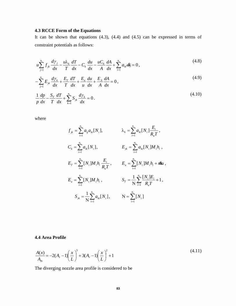
83
4.3 RCCE Form of the Equations It can be shown that equations (4.3), (4.4) and (4.5) can be expressed in terms of
constraint potentials as follows:
∑ ∑= =
=+−−−c sn
j
n
iiik
kk
kjjk a
dx
dA
A
uC
dx
duC
dx
dT
T
u
dx
dfu
1 1
0ωγ
&λ,
(4.8)
∑=
=+++−cn
j
AuTkk dx
dA
A
E
dx
du
u
E
dx
dT
T
E
dx
dE
1
0γ
γ , (4.9)
∑=
=+−cn
k
kk
T
dx
dS
dx
dT
T
S
dx
dp
p 1
01 γ
γ . (4.10)
where
∑=
=sn
iiikijjk Naaf
1
],[ ∑=
=sn
i u
iiikk TR
ENa
1
][λ ,
∑=
=sn
iiikk NaC
1
][ , ∑=
=sn
iiiikik hMNaE
1
][γ ,
∑=
=sn
i u
iiiiT TR
EhMNE
1
][ , umhMNEsn
iiiiu &+=∑
=1
][ ,
∑=
=sn
iiiiu hMNE
1
][ , ∑=
+Ν
=sn
i u
iiT TR
ENS
1
1][1
,
∑=Ν
=sn
iikik NaS
1
][1
γ , ∑=
=Νsn
iiN
1
][
4.4 Area Profile
The diverging nozzle area profile is considered to be
1)1(3)1(2)(
23
+
−+
−−=
L
xA
L
xA
A
xArr
th
(4.11)

84
where
th
endr A
AA =
The length of the nozzle, L, has been non-dimensionalized with respect to the height of
the throat section.
4.5 Constraints Selection of constraints is certainly the most important aspect of RCCE, on which
a successful application of the method depends. Among the general requirements for the
constraints are that they must (a) be linearly independent combinations of the species
mole numbers, (b) hold the system in the specified initial state, (c) prevent global
reactions in which reactants or intermediates go directly to products, and (d) determine
the energy and entropy of the system within experimental accuracy. In addition, they
should reflect whatever information is available about rate-limiting reactions which
control the evolution of the system on the time scale of interest.
A new algorithm based on the degree of disequilibrium (DOD) of chemical
reactions has been proposed to select constraints. The DOD of reaction k is defined as
−
+
=k
kk r
rlnφ
(4.12)
This physical quantity serves as the driving force for reaction k and generates the
reaction flux rk=r k+-rk
-. The quantity rk φk determines the amount of entropy produced by
reaction k, which is obviously non-negative. If a reaction has a DOD equal or close to
zero, depending on the value of either forward or reverse reaction rates, it can be either
very slow or at partial equilibrium.
As stated earlier in the previous section, a reaction is in constrained equilibrium only if it
does not change any of the constraints. Equivalently, if a reaction or classes of reactions
are judged to be in constrained equilibrium, either by user's knowledge of chemistry or by
a mathematical algorithm, they imply one or several constraints of varying degrees of
effectiveness. The conjecture here is that the smaller the DOD of a reaction or groups of
reactions, the more valid the assumption of constrained equilibrium for such reactions.

85
This assumption subsequently implies a set of constraints, it a subset or all of which may
be sufficient to describe the system to within the accuracy of experimental data or a
DKM. So far this conjecture has been tested for relaxations away from an equilibrium
state.
4.6 Results and discussions
4.6.1 H/O Reacting System
The nozzle considered is a diverging nozzle and has an exit-to-throat area ratio of 50.
The length of the nozzle is assumed to be ten times the height of the throat section. The
initial condition corresponds to a Mach number of 1.01 and temperature and pressure of
3200K and 25atm, respectively. The kinetic mechanism involves 8 species and 24
reactions. Figure 4.1 presents the DOD for reactions in the mechanism.
x (along the nozzle)
φ i
0 2 4 6 8 10-1
0
1
2
3
4
5
6
7
8
9
10
11
3B. Rxns: 1,2,3,4,5,6
3B. Rxns: 7,8,9,10
2B. Rxns: 12,15,16,17,19,22,24
2B. Rxns: 11,13,14,18,20,21,23
Figure 4.1: Degree of disequilibrium (DOD) for reactions involved in the kinetics
Several interesting observations can be made in figure 4.1. The first observation is
that all three-body reactions are far from equilibrium, confirming the previously

86
discovered structural constraint on total number of moles, which controls the dynamics
of molecule formation and the change in the total number of particles in the system [7]. It
is also compatible with the physics of expansion that when a highly dissociated mixture
expands to lower gas temperatures and densities three body recombination dynamics
becomes an important part of the restoration process, in accordance with the Le Chatelier
principle. The second observation is that the three body reactions can further be divided
in to two groups based on their DOD’s. This suggests that the group with lower DOD
may be of secondary importance within the three-body dynamics. Three body reactions
are listed below:
The first 6 reactions are obviously the most important ones in molecule formation,
which are directly related to the major species. Given the importance of the H/O
dynamics in all starting-from-equilibrium relaxations, it is anticipated that the same set of
reactions, R1-R6, would control the major dynamics under total number of moles, if M
were proved to be a rate-controlling constraint. The third interesting observation made in
figure 4.1 is that a subset of bi-molecular reaction dynamics remains close to constrained
equilibrium throughout the relaxation. These reactions are listed below:
These reactions are the ones assumed in constrained equilibrium. As explained under
section 2.2, the assumption of constrained equilibrium implies constraints which are
unchanged by these reactions. A little scrutiny reveals the following groupings: c1 ≡
R1. O+O+M=O2+M
R2. O+H+M=OH+M
R3. H+H+M=H2+M
R4. H+H+H2=H2+H2
R5. H+H+H2O=H2+H2O
R6. H+OH+M=H2O+M
R7. O+O2+M=HO2+M
R8. O+O2+O2=HO2+O2
R9. O+O2+H2O=HO2+H2O
R10. OH+OH+M=H2O2+M
R11. O+H2=H+OH
R13. O+H2O2=OH+HO2
R14. H+O2=O+OH
R18. H+H2O2=HO2+H2
R20. OH+H2 =H+H2O
R21. OH+OH =O+H2O
R23. OH+H2O2=HO2+H2O

87
H+H2 based on R11, R18, R20, c2 ≡ O+OH based on R11, R13, c3 ≡ HO2+H2O2 based on
R13, R18 and R23 and c4 ≡ OH+H2O based on R20, R23. Interestingly, combining c2 and
c4 and forming c5 ≡ O+OH+H2O leaves their corresponding reactions intact, yet puts
reactions R21 in constrained-equilibrium as well, which further means reduction of the
number of constraints by one!
Based on the foregoing analysis the following table of constraints is suggested by
constrained-equilibrium reactions:
Table 4.1: Constraints implied only by examining the constrained-equilibrium reactions
Constraints Based on reactions
C1 ≡ H+H2 R11, R18, R20
C2 ≡ O+OH+H2O R11, R13,R20,R23
C3 ≡ HO2+H2O2 R13, R18 and R23
Two yet more interesting observations can be made from Table 4.1 and the constrained-
equilibrium reactions. The C2 group is the previously discovered structural constraint of
Free Oxygen and all constrained-equilibrium reactions, except reaction R14, conserve
another not-easy-to-observe structural constraint, namely Free Valence. One extra
observation is that Reaction R14 not only does not suggest any consistent constraint, it
further does not conserve any of the constraints in Table 4.1. Calculations, as presented in
figure 4.2, show that, although known to be important, elimination of this reaction results
in agreements with DKM to within 0.2% of accuracy throughout. Obviously this
elimination is only valid over the range of thermodynamic conditions that the reaction
shows the behavior of a constrained-equilibrium reaction. In figure 4.2, the RCCE (DOD)
designates the calculations under Table 4.1 in addition to elemental constraints. RCCE-
Shifting Equilibrium corresponds to local thermodynamic calculations subject to
elemental constraints only and RCCE - Frozen Equilibrium designates calculations in
which each species forms a conserved constraints. The difference between RCCE(DOD)
and DKM is consistently less than 0.06% throughout.

88
An important question at this stage is the relation between the set presented in
Table 4.1 and the structural constraints, M and FV. In what follows we show that these
are not linearly independent. By definition the elemental oxygen can be written as:
EO = FO+2(H2O2+HO2)+2O2=C2+2C3+2O2 (4.13)
In which FO is free oxygen. Also, the total number of moles, M, is defined as:
M = (H+H2)+(O+OH+H2O)+(HO2+H2O2)+O2 = C1+C2+C3+O2 (4.14)
Substituting similar terms from (2) into (3), one gets:
M = C1+1/2(EO+C2) (4.15)
x (along the nozzle)
Tem
per
atur
e(K
)
0 2 4 6 8 10
1000
1500
2000
2500
3000 RCCE - Shifting Equilibrium (EO,EH)RCCE (DOD)DKMRCCE - Frozen Equilibrium
Figure 4.2: RCCE predictions under Table 4.1 compared with DKM, shifting equilibrium and frozen equilibrium.

89
Relations (4.13) and (4.15) clearly establish the linear dependence of M and O2 on
constraints in Table 4.1. It can also be shown that M and FV are related to O2 and
elemental Hydrogen, EH, in the following form:
(M-O2) - FV/2 = EH/2 (4.16)
Substituting from the second equality of relation (49) into (51), one obtains:
2(C1+C2+C3) – EH = FV (4.17)
x (along the nozzle)
Log
(Mol
eF
ract
ion)
0 2 4 6 8 10-3.5
-3
-2.5
-2
-1.5
-1 DKMRCCE
H2
OH
H
O2
O
x (along the nozzle)
Log
(Mol
eF
ract
ion)
0 2 4 6 8 10-3.5
-3
-2.5
-2
-1.5
-1 DKMRCCE
H2
OH
H
O2
O
x (along the nozzle)
Lo
g(X
O2)
0 2 4 6 8 10-8
-7
-6
-5
-4
-3
-2
-1
DKMRCCE - LTERCCE - HPORCCE - FORCCE - HH2RCCE - HH2+FORCCE - HH2+FO+HPO
x (along the nozzle)
Log
(XH
2O)
0 2 4 6 8 10-0.07
-0.06
-0.05
-0.04
-0.03
-0.02
-0.01
0
DKMRCCE - LTERCCE - DOD
Figure 4.3: The DOD predictions of species profiles compared with those of DKM along
the axis of the nozzle. Also (d) shows a systematic improvement in predictions by adding
constraints one at a time.
(a) (b)
(c) (d)

90
Relations (4.15) and (4.17) mathematically demonstrate that M and FV can substitute C1
and C2 with no change in predictions at all. All calculations show exact same predictions
for the set (M, C2, FV) which is basically the generalized set (M, FO, FV).
4.7 RDX Reacting System
The same methodology was applied to expansion of RDX combustion products
through a supersonic nozzle. Calculations show that the high pressure keeps the mixture
at the corresponding local thermodynamic equilibrium at each point up to the throat
section, beyond which kinetic effects emerge. Therefore, the boundary condition at the
throat section corresponds to an equilibrium mixture at a Mach number of 1.0. The
corresponding temperature profiles are shown for different constraints in figure 4.3.
x (along the nozzle)
Tem
per
atu
re(K
)
0 2 4 6 8 10
600
900
1200
1500
1800
2100
2400
2700
3000
3300Local Thermody. EquilibriumRCCE (FN)RCCE (M)RCCE (DCO)RCCE (M,FO)RCCE (M,FV,FO,FN)DKMFrozne Equilibrium
Figure 4.4: The RCCE prediction of temperature profile during expansion of combustion products through a supersonic nozzle.
As is evident from figure 4.4, the only kinetic constraint required in this case is DCO to
match the predictions of the detailed kinetic model. This means only one differential rate
equation for the kinetic constraints, a considerable reduction in the number of differential

91
rate equations to be solved! An interesting observation is that the recombination
dynamics is completely in equilibrium. Contrary to the consensus in the community,
when taking into account the residence time of 1.2×10⁻⁴sec within the nozzle, it
demonstrates that all three body reactions are equilibrated.
Acknowledgment
This research was financially supported by Army Research Office (ARO) under technical monitoring of Dr. Ralph Anthenien.
4.8 References [1] Keck, J. C., Gillespie, D., 1971, Combustion and Flame, Vol. 17, pp. 237. [2] Keck, J.C., 1990, Prog. Energy Combust. Sci., Vol. 16 pp. 125. [3] Bishnu, P., Hamiroune, D., Metghalchi, M., and Keck, J.C., 1997, Combust. Theory and Modeling, Vol. 1, pp. 295-312. [4] Hamiroune, D., Bishnu, P., Metghalchi, M. and Keck, J.C., 1998, Combust Theory and Modeling, Vol. 2, pp. 81. [5] Tang, Q., Pope, S. B., 2004, Combus Theory and Modeling, Vol., 8 pp. 255 - 279. [6] Jones, W. P., Rigopoulos, S., 2005, Combust. Flame, Vol. 142 pp. 223– 234. [7] Janbozorgi, M., Ugarte, S., Metghalchi, H., Keck, J. C., 2009, Combust. Flame, 156 (10), [8] Yousefian, V., 1998, Combus Flame, Vol. 115, Issues 1-2, , pp: 66-80 [9] Hiremath, V., Ren, Z., Pope, S. B., 2010, Combust. Theory Modeling, 14(5), 619- 652. [10] Bray K.N.C., 1958, Atomic recombination in a hypersonic wind-tunnel nozzle, Journal of Fluid Mechanics, 6, pp: 1-32

92
Chapter 5
93
Conclusions and Future Works

94
5.1 Conclusions
The RCCE method was developed to study the oxidations of methane, methanol and
formaldehyde over a wide range of initial temperatures and pressures. In this regard, a set
of up to 12 total constraints (elemental + kinetic) were identified, which result in
excellent agreements with “detailed”-kinetic-model (DKM) calculations using 29 species
and the same set of 133 reactions. In addition, reduced sets of 20 reaction for methane, 12
reactions for methanol and 12 reactions for formaldehyde have been found, which when
employed in the RCCE calculations give results identical to those obtained using the full
133 reactions. Also, it was shown that a subset of these constraints, termed as generalized
or universal constraints, is able to reproduce the chemical kinetic features of the
expansion dynamics in an internal combustion engine and in a supersonic nozzle.
Among the important features of the RCCE method for simplifying the kinetics of
hydrocarbon oxidation are:
1. It is based on the well established Maximum Entropy Principle of
thermodynamics rather than mathematical approximations.
2. The entropy always increases as the system evolves and an approach to the
correct final chemical-equilibrium state for the specified elements is
guaranteed. This is not true for DKMs where only the listed species are
included and all others are missing.
3. The total number of constraints required to describe the state of a complex
chemical system can be very much smaller than the number of species in the
system resulting in fewer equations.
4. It enables one to obtain a good description of the kinetic behaviour of a
complex chemically reacting system using a relatively small number of
constraint-controlling reactions without having to start with a DKM.
95
5. An estimate of the concentrations of any species for which the standard Gibbs
free energy is known can be obtained even though the species is not explicitly
included in the model used.
6. If the only constraints on the system are the elements and the state variables,
RCCE calculations reduce to local equilibrium (LTE) calculations.
7. If the species are used as constraints, RCCE calculations simulate DKM
calculations with the important distinction that only the listed species can
appear in DKM calculations whereas all possible species are implicitly
included in RCCE calculations.
8. The accuracy of the results can be systematically improved by adding
constraints one at a time.
96
5.2 Future Works
Future works on RCCE could be carried out in two very exciting and currently
demanding fields: a) inclusion of diffusion fluxes and studying the RCCE structure of
laminar and turbulent flames, b) using RCCE in a bottom-up approach to build kinetic
models for heavy hydrocarbon fuels. Furthermore, an important observation throughout
the course of this thesis was that using groups of species as constraints results in
sometimes stiff RCCE calculations, such that the overall time saving is minimal. From
the modelling stand point, which has been the focus of this thesis, grouping species as
constraints offers the exceptional feature of identifying the oxidation pattern that could be
further extended to heavy hydrocarbons. However, optimized numerical algorithms must
be developed to further reduce the CPU time. A reduction in the CPU time proportional
with the considerable reduction in the number of equations would make the RCCE a very
promising method for kinetic simplification.