Transport simulations in nanosystemsand low-dimensional systemsVon der Fakultät für Mathematik und Physikder Gottfried Wilhelm Leibniz Universität Hannoverzur Erlangung des GradesDOKTOR DER NATURWISSENSCHAFTENDr. rer. nat.genehmigte DissertationvonDipl. Phys. Mal olm Einhellingergeboren am 13.09.1980 in Wolfsburg.

2013

Referent: Prof. Dr. Eri Je kelmannKorreferentin: Prof. Dr. Gertrud Zwi knaglTag der Promotion: 14.11.2012

3

4Abstra tIn this thesis, we investigate the transport properties of low-dimensional orrelated nanosystems. Even though we an not simulate low-dimensionalnanosystems in their full experimental reality, we approa h this goal in threesu essive steps, extending the basis for future theoreti al and experimentaltransport studies.In the rst step, we investigate one-dimensional ondu tors, i.e. the spin-less fermion model and the Hubbard model. In that regard, we use the timeevolving blo k de imation (TEBD) method to simulate nite systems drivenout of equilibrium by an applied potential bias. Using the Fourier analysisbased extra tion (FABE) method a pro edure whi h we have developedbased on the analysis of a related lassi al model (LC line) we are ableto al ulate the stationary urrent using the results of the TEBD simula-tions of systems with a nite size. We show the full IV hara teristi s ofthe one-dimensional spinless fermion model with nearest-neighbor Coulombintera tion VH and several IV hara teristi s of the one-dimensional Hub-bard model with onsite Coulomb intera tions UH, using two dierent setupsto generate urrents (turning on/o a potential bias).Sin e in an experimental situation latti e vibrations play an importantrole, in the se ond step we investigate the appli ability of the TEBD methodto nanostru tures oupled to a bosoni bath. As TEBD has never beenapplied to su h systems before, we have to ompare our results with thosefrom well-established methods su h as the numeri al renormalization group(NRG) pro edure. Thus, we hoose a two-site fermioni system oupled toa bosoni bath, for whi h NRG al ulations are available, and nd that theTEBD results agree with the NRG data.In the third step we take into a ount that realisti nanowires are notexa tly one-dimensional but their band stru ture onsists of several one-dimensional subbands. To over those ases, we modify the TEBD ode su hthat it an be applied to two-dimensional stru tures, and simulate a lad-der system des ribed by the tight-binding Hamiltonian. Exa t results fromone-parti le equation of motion al ulations onrm our TEBD simulationout omes.Keywords: TEBD, low-dimensional orrelated nanosystems, stationary ur-rent

5ZusammenfassungIn dieser Arbeit untersu hen wir die Transporteigens haften von niedrigdi-mensionalen, korrelierten Nanosystemen und wie die theoretis hen Ergeb-nisse experimentell gemessen werden können. Obwohl wir keine niedrigdi-mensionalen Nanosysteme in ihrer vollständigen, experimentellen Umgebungsimulieren können, nähern wir uns dieser Zielsetzung in drei aufeinanderfol-genden S hritten. Dadur h erweitern wir die Basis für zukünftige theoretis- he und experimentelle Studien.Im ersten S hritt untersu hen wir eindimensionale Leiter, insbesondere dasspinlose Fermionen Modell und das Hubbard Modell. In diesem Zusammen-hang benutzen wir die zeitentwi kelte Blo kdezimierungsmethode (TEBD)um endli h groÿe Systeme im dur h ein externes Potential erzeugten Ni ht-glei hgewi ht zu simulieren. Mit Hilfe der Fourieranalyse basierten Extrak-tionsmethode (FABE) einer Prozedur die wir mittels Analyse eines ver-wandten klassis hen Modells (LC Modell) entwi kelt haben sind wir in derLage den stationären Strom anhand der TEBD Simulationen eines endli hgroÿen Systems zu bere hnen. Wir zeigen die vollständigen IV Eigen-s haften des eindimensionalen spinlosen Fermionen Modells mit nä hster-Na hbar Coulomb-We hselwirkung VH und zudem IV Eigens haften deseindimensionalen Hubbard Modells mit Vor-Ort Coulomb-We hselwirkung|UH| mit Hilfe zweier Setups zur Erzeugung eines Stromes (An-, bzw. Ab-s halten der angelegten Spannung).Da in einer experimentellen Umgebung besonders Gitters hwingungen einewi htige Rolle spielen, untersu hen wir im zweiten S hritt die Anwendbarkeitder TEBDMethode auf Nanostrukturen wel he an ein bosonis hes Bad gekop-pelt sind. Da zudem TEBD niemals zuvor auf sol he Systeme angewen-det wurde, müssen zunä hst Verglei he mit etablierten und auf dieses Prob-lem optimierten Methoden, wie zum Beispiel die Methode der numeris henRenormalisierungsgruppe (NRG) angestellt werden. Daher wählen wir einfermionis hes Zwei-GitterplatzModell, wel hes an ein bosonis hes Bad gekop-pelt ist, und für das NRG Re hnungen verfügbar sind. Dabei erhalten wireine Übereinstimmung der TEBD- mit den NRG-Daten.Im dritten S hritt berü ksi htigen wir, dass realistis he Nanodrähte ni htwirkli h eindimensional sind, sondern dass ihre Bandstruktur aus vielen eindi-mensionalen Teilbändern aufgebaut ist. Um diese Situationen abzude ken,wird zunä hst der TEBD-Code so modiziert, dass er auf zweidimensionaleSysteme angewandt werden kann. Ans hlieÿend simulieren wir ein Leitersys-tem wel hes dur h den tight-binding Hamiltonoperator bes hrieben wird. Dieexakten Ergebnisse aus Einteil hen-Bewegungsglei hungs-Re hnungen bestä-tigen unsere TEBD Ergebnisse.

6S hlagworte: TEBD, niedrig-dimensionale korrelierte Nanosysteme, stationärerStrom

Contents 7ContentsChapter 1. Introdu tion 9Chapter 2. Classi al LC line 152.1 Currents in the LC line . . . . . . . . . . . . . . . . . . . . . . 162.2 Stationary urrent . . . . . . . . . . . . . . . . . . . . . . . . 202.3 Finite-time and nite-size ee ts . . . . . . . . . . . . . . . . . 222.4 Determining the stationary urrent from nite system values . 252.5 Charge distribution . . . . . . . . . . . . . . . . . . . . . . . . 292.6 Final notes on the LC line . . . . . . . . . . . . . . . . . . . . 312.6.1 Setups . . . . . . . . . . . . . . . . . . . . . . . . . . . 312.6.2 Applying the FABE approa h to re tangular signals . . 312.7 Summary . . . . . . . . . . . . . . . . . . . . . . . . . . . . . 33Chapter 3. Non-equilibrium simulations 353.1 Tight-binding model . . . . . . . . . . . . . . . . . . . . . . . 353.2 Setups . . . . . . . . . . . . . . . . . . . . . . . . . . . . . . . 363.3 One-parti le equation of motion . . . . . . . . . . . . . . . . . 383.4 Finite-size ee ts and stationary urrent . . . . . . . . . . . . 413.4.1 Finite-size indu ed os illation . . . . . . . . . . . . . . 413.4.2 Rapid os illation on top of the square wave . . . . . . . 433.4.3 Appli ability of the FABE approa h to quantum systems 463.5 Summary . . . . . . . . . . . . . . . . . . . . . . . . . . . . . 48Chapter 4. TEBD method 514.1 Parallelization . . . . . . . . . . . . . . . . . . . . . . . . . . . 544.2 Error sour es . . . . . . . . . . . . . . . . . . . . . . . . . . . 564.3 Notes on the omputation of stationary urrents . . . . . . . . 574.4 Summary . . . . . . . . . . . . . . . . . . . . . . . . . . . . . 58Chapter 5. Spinless fermion model 595.1 Simulation parameters and errors . . . . . . . . . . . . . . . . 615.2 Simulation results . . . . . . . . . . . . . . . . . . . . . . . . . 625.2.1 Current-voltage hara teristi s . . . . . . . . . . . . . . 625.2.2 Inuen e of VH on the period Tmax . . . . . . . . . . . 68

8 Contents5.3 Summary . . . . . . . . . . . . . . . . . . . . . . . . . . . . . 69Chapter 6. Hubbard model 716.1 Simulation parameters, modi ations and errors . . . . . . . . 726.2 Simulation results . . . . . . . . . . . . . . . . . . . . . . . . . 736.2.1 Equilibrium onsite potentials . . . . . . . . . . . . . . 736.2.2 Current-voltage hara teristi s . . . . . . . . . . . . . . 756.3 Summary . . . . . . . . . . . . . . . . . . . . . . . . . . . . . 77Chapter 7. Two-site system oupled to a bosoni bath 797.1 Two-site fermioni system in a bosoni bath . . . . . . . . . . 807.1.1 Mapping to a semi-innite hain . . . . . . . . . . . . . 817.1.2 General simulation parameters . . . . . . . . . . . . . . 837.2 Simulation results . . . . . . . . . . . . . . . . . . . . . . . . . 847.2.1 Equilibrium properties . . . . . . . . . . . . . . . . . . 847.2.2 Realtime dynami s . . . . . . . . . . . . . . . . . . . . 867.3 Summary . . . . . . . . . . . . . . . . . . . . . . . . . . . . . 88Chapter 8. Ladder systems 918.1 Tight-binding ladder system . . . . . . . . . . . . . . . . . . . 928.2 Simulation parameters and errors . . . . . . . . . . . . . . . . 928.3 Simulation results . . . . . . . . . . . . . . . . . . . . . . . . . 938.4 Summary . . . . . . . . . . . . . . . . . . . . . . . . . . . . . 95Chapter 9. Summary, Con lusion & Outlook 979.1 Summary & Con lusion . . . . . . . . . . . . . . . . . . . . . 979.2 Outlook . . . . . . . . . . . . . . . . . . . . . . . . . . . . . . 99Appendix A. LC line 101A.1 Current in the nite LC line . . . . . . . . . . . . . . . . . . . 101A.2 Solution of the integral (2.24) . . . . . . . . . . . . . . . . . . 103A.3 Solution of the integral (2.32) . . . . . . . . . . . . . . . . . . 103A.4 Approximations of the Bessel and Struve fun tions . . . . . . 104A.5 Remainder approximation for the Taylor series expansion . . . 105Appendix B. Non-equilibrium simulations 109B.1 Perturbation theory for small and large biases . . . . . . . . . 109B.2 Period of the re tangular os illation in the tight-binding model 110B.3 Current in the innite tight-binding model . . . . . . . . . . . 111Appendix C. TEBD update s heme 113

9Chapter 1Introdu tionOur understanding of ele troni transport in one-dimensional ondu tors ispartly based on experimental out omes su h as for instan e the transportthrough single-walled arbon nanotubes whi h rst showed up in 1991 [1.The rst transport experiment for those stru tures, whi h an be down toa few nanometers in diameter, has then been reported in 1997 [2, 3 wherea potential bias has been applied to two leads (referred to as sour e anddrain) onne ted to the nanotube, and the resulting urrent through thenanotube has been measured. Due to the small diameter of those stru tures,they are often onsidered to be one-dimensional, but in fa t the band stru -ture is omposed of multiple one-dimensional subbands. Thus, ele troni orrelations are important and the Fermi liquid theory for normal ondu -tors an not be applied. A ording to the Tomonaga-Luttinger liquid (TLL)theory [4, 5, 6, 7, for the experimental setup of a nanotube onne ted to omparably innitely large sour e and drain, a quantized ondu tan e of

4e2/h for ea h subband is predi ted, whi h has been su essfully measuredfor metalli nanotubes [8. Various other pseudo one-dimensional stru tureshave been prepared and investigated, su h as for instan e metalli atomi hains on surfa e substrates [9, or stru tures based on anisotropi (for in-stan e stepped) surfa es.While experimentalists have to work hard to prepare su h stru tures, the-oreti ians have it by far easier in one dimension. By ontrast, it is quitea hallenge to get theoreti al results for transport problems in luding theinnitely large reservoirs used in experimental setups, and thus theoreti alinvestigations on transport in one dimension are often restri ted to nitesystem sizes (see for instan e [10, 11 for simulations of nite systems), andsour e and drain are often modeled as part of the one-dimensional stru -ture. Although the transport properties of one-dimensional ondu tors havebeen investigated both numeri ally and theoreti ally [12, 5, 7, 13, 14, 15,most of those studied are restri ted to either small applied potential biases(`small' ompared to the order of the band width in latti es and to the Fermivelo ity in ontinuous models) or small Coulomb intera tions, treating theele tron-ele tron intera tion pertubatively.

10 Chapter 1. Introdu tionThe transport properties of those systems for applied biases whi h areweak ompared to the energy s ale of the system are des ribed by the TLLtheory and exa t equilibrium properties are available from Bethe Ansatzsolutions for instan e for the spin 12XXZ hain in Bethe's original work [16(and losely related the spinless fermion model), the Kondo model and theHubbard model [17, 18. Without Coulomb intera tions, exa t results arealso available for higher applied voltages [15.The nonlinear regime has mostly been investigated in quantum onta tproblems, where the intera tion is onned to a small region of the system,su h as the Kondo model or the intera ting resonant level model (IRLM).Within the framework of the TLL theory, urrent-voltage hara teristi s havebeen studied for the transport through a weak link [19, 20, for instan e a one-dimensional intera ting fermion system for a weak or strong potential barrier.Re ently, the ee ts in the nonlinear regime have also been investigated [21,and a few works on erned with the full IV hara teristi s showed up [22,11, 24. Again, their interest lies mainly on systems with a small intera tingregion onne ted to non-intera ting leads, su h as the IRLM or the singleimpurity Anderson model (SIAM) and none on entrates on one-dimensional orrelated ondu tors, i.e. where the Coulomb intera tion is present in thewhole system.A major goal of this thesis is to investigate, determine and understand thenonlinear transport properties of low-dimensional orrelated ondu tors inwhi h the Coulomb intera tion is not onned to a small region but presentin the whole system. As ele troni s on a nanos ale has be ome more inter-esting in re ent years, it is important to gain a better understanding of thosepro esses to reveal the full s ope of quantum wires as ele troni omponents.In this thesis, we do not try to reprodu e a spe i experimental situation,but to generally understand ee ts in orrelated one-dimensional ondu tors.For that, our approa h is to study a nanowire whi h is either itself hargedsu h that parts of the nanowire a t as sour e and drain or (more relatedto an a tual experimental situation) to whi h an external voltage is applied.Nevertheless, several experimental aspe ts an not be ignored. Among many,the following three are the most important ones. First, many nanowireshave a length-to-diameter ratio of 1000 and more, thus ex eeding the presentnumeri al possibilities. Se ond, a nanowire is not stri tly one-dimensionalbut its band stru ture rather onsists of multiple one-dimensional subbands,and third, latti e vibrations have to be taken into a ount. The onne tionof the nanowire to a surfa e and its oupling to leads is not onsidered in thisthesis. Therefore, this thesis onsists of three major parts: the investigationof one-dimensional orrelated ondu tors, the study of a system oupled toa bosoni bath, and a resear h on the appli ability of our methods to low-

11dimensional quantum systems.In the rst and major part we study one-dimensional ondu tors, i.e.the half-lled spinless fermion model and the Hubbard model away fromhalf-lling. Even though both models are exa tly solvable by the BetheAnsatz and their properties for small applied biases are des ribed by theTLL theory, their transport properties in the nonlinear regime are not ana-lyti ally a essible. Thus, we use the time evolving blo k de imation (TEBD)method [25, 26 to simulate the nite systems driven out of equilibrium us-ing two dierent setups. In the rst setup (I) we initially (at time t = 0)apply a potential bias to sour e and drain (the two halves of the system).For t > 0 we let the system evolve without potential bias and measure the urrent owing through the bond between sour e and drain. In the se ondsetup (II) for t = 0 we prepare the system without a potential bias and applya voltage for t > 0, whi h also generates a urrent. We again measure the urrent through the bond between sour e and drain.Re ently, several numeri al methods for simulating the realtime dynam-i s of quantum latti es have been developed [27, 28, 29, su h as for instan ethe time-dependent density matrix renormalization group (td-DMRG) or theTEBD method. Both methods an be des ribed within a ommon mathe-mati al framework, the matrix produ t states (MPS) [29, 30, 31. The greatadvantage of the MPS des ription is the possibility to keep only the most`relevant' states and dis ard all others. Fortunately, the ontribution of ea hstate de ays very qui kly, su h that a rather small number χc of states (theS hmidt dimension) has to be kept to get a urate results. However, asthe entanglement in the system rises, χc rises as well, thus dening thelimit of what an be simulated anyway. The td-DMRG method has beensu essfully applied to study transport properties in quantum latti e sys-tems [22, 11, 32, 33, 34, 10, 35, 23, 36, 37, 38, su h as for instan e thementioned SIAM, the IRLM or the Hubbard model and the spinless fermionmodel, even for strong orrelations (see for instan e [39). However, the orig-inal TEBD method has not yet been applied to ele troni transport problemsat all.Although the use of the TEBD method is restri ted to low-dimensionalsystems, it has a great advantage over the td-DMRG method. While theparallelization or the DMRG pro edure is quite ompli ated [40, 41, TEBDis naturally parallelizable with an extremely low overhead, whi h will bepresented in hapter 4 in this thesis. Using the TEBD method, we are ableto ompute the ground state and simulate the realtime evolution of a nitesystem of size N for a nite time t. Using one of the two setups des ribedabove, the system rst goes into a transient phase in whi h a noisy andos illating urrent is owing. As the os illations be ome smaller, the urrent

12 Chapter 1. Introdu tionapproa hes a onstant value while the system goes into a quasi-stationaryphase whi h is ontinued until the parti le front wave hits one of the bordersof the system.Sin e we are interested in the stationary behaviour of larger stru turesand espe ially in the DC transport properties (of innitely large systems),we have to extrapolate the simulation results to the limits N →∞ and thent→∞. As nite-size ee ts in quantum systems are very omplex [42 andsin e we know only little about the inuen e of the borders in nite systemson the quasi-stationary urrent, we rst study a related lassi al mode, theso- alled LC line. With the aid on our ndings, we develop a Fourier analysisbased extra tion (FABE) method, whi h allows us to al ulate the stationary urrent in innitely large systems using numeri al data from small systemsand short simulation times, for instan e our TEBD simulation results.Using TEBD and the FABE method, we determine the full IV hara ter-isti s of the spinless fermion model and IV hara teristi s of the Hubbardmodel. Without Coulomb intera tion, these models are exa tly solvable usingthe one-parti le equation of motion formalism, and for small applied potentialbiases predi tions from the TLL theory are available. All results from thesespe ial ases onrm the validity of our approa h. We nd that while for thelinear regime the spe i setup does not matter, it is highly de isive for thenonlinear urrent-voltage hara teristi s. For setup (I) the system shows apositive dierential ondu tan e all over the full voltage range and saturatesat a nite value. For setup (II) a negative dierential ondu tan e o ursfor higher applied voltages, even impeding a urrent ow for large enoughvalues. Both ee ts in setup (II) that also o ur in the non-intera ting ase, ome from the nite bandwidth and the nonlinear dispersion of the ex ita-tions [42, 43.As already mentioned, latti e vibrations (generally dissipation) play animportant role in experimental situations. Thus in the se ond part of thisthesis, we study the appli ability of the TEBD method to systems oupledto a bosoni bath. For that purpose we hoose a model that an be analyzedusing TEBD and for whi h highly a urate (TD) NRG ((time dependent)numeri al renormalization group) simulation results are available for om-parison: a two-site fermioni system oupled to a bosoni bath [44. Thismodel des ribes the essentials of a two-ele tron transfer in a dissipative envi-ronment, whi h has been suggested to be an important me hanism in manybiologi al pro esses, for instan e in DNA [45.Up to the present day, both methods, TEBD and NRG have been usedto al ulate the ground states and realtime dynami s of quantum systems,but a dire t omparison has not been yet arried out. While (TD) NRGis well-suited for su h simulations, providing very a urate des riptions for

13small quantum systems oupled to a bosoni bath, TEBD an in prin iplebe used for even more extended impurities, su h as large mole ular bridgesor nanowires. Our analyses show that even though the TEBD results agreewith the NRG out omes, it is very hard to simulate the ground state sin e avery high S hmidt dimension is needed to get a su iently small trun ationerror. Moreover, even though the realtime evolution needs only a reasonablysmall S hmidt dimension, unfortunately a very small time step is ne essaryto obtain a urate results, whi h is due to very long time s ales in whi h thetransfer pro esses in this model take pla e.In the third part of this thesis we extend the TEBD method in view ofthe fa t that realisti nanowires are not truly one-dimensional. It is basi allypossible to use TEBD also for higher-dimensional systems by building anee tively one-dimensional system. With this mapping strategy, we use theTEBD method to simulate a ladder system whi h is des ribed by the tight-binding Hamiltonian. We use the two setups des ribed above in dierent waysand nd by omparison with one-parti le equation of motion al ulationsthat the TEBD method gives orre t results for su h systems. It neverthelessremains a hallenge to apply TEBD to two-dimensional systems with a widerextent.This thesis is organized as follows: In the next hapter we introdu e the lassi al LC line and the extra tion method (FABE) used in the following hapters. We study several nite-size and nite-time ee ts of the lassi almodel, deriving many of its properties, su h as the period of the re tangularos illation, or the origin of a rapid os illation on top of the quasi-stationaryplateau. In the third hapter we investigate stationary and transient ur-rent properties in a quantum tight-binding model, applying the one-parti leequation of motion method and the FABE method from the se ond hap-ter. Based on the lose onne tion to the lassi al LC line we show theappli ability of the FABE method to quantum systems. The fourth hapterexplains how we have implemented the parallel TEBD method and what er-rors are to be expe ted for the following simulations. In the fth and sixth hapter we apply our methods to the spinless fermion model and the Hub-bard model. We obtain the full IV hara teristi s of the spinless fermionmodel (in luding a negative dierential ondu tan e and saturation ee ts).Moreover, we show that the period of the spinless fermion model for dierentVH hanges only due to the nite renormalized band width. Our investiga-tions on the Hubbard model reveal IV hara teristi s for one setup whi hshow a similar saturation of the urrent as for the spinless fermion model.For des ribing a one-dimensional system in an experimental environment, wehave to take latti e vibrations into a ount. The TEBD method is thereforeadapted and used to simulate the two-site fermioni system oupled to a

14 Chapter 1. Introdu tionbosoni bath in the seventh hapter and omparisons with NRG results [44are arried out. As the band stru ture of a realisti nanotube onsists ofmultiple one-dimensional subbands, we simulate a ladder system des ribedby the tight-binding model using TEBD in the eighth hapter.All important (in this thesis) realized implementations, al ulations andndings are summarized in the last se tion of ea h hapter. Finally, wesummarize all of our ndings and give an outlook for further work in theninth hapter. Some al ulations are listed in appendi es.

15Chapter 2Classi al LC lineIn this hapter we start with the investigation of nite-size and nite-timeee ts in lassi al os illator-systems to explain orresponding ee ts in sim-ulation results from quantum systems. Classi al os illator-systems typi ally onsist of ma ros opi elements, su h as a mass-spring system or more ele -troni ally an LC-Line built upon ondensators, indu tors and maybe resis-tors. Some lassi al setups are furthermore omparable to quantum me han-i al systems, regarding for instan e parti le densities and urrents. Those lassi al setups are in most ases easier to des ribe and the orrespondingmodels more often solvable than their quantum me hani al pendants. Fur-thermore, they open the way to understanding the origin of quantum ee tsand they are a useful tool for gaining more informations about quantum sys-tems, for instan e by omparing model parameters and simulation results.In the following, we on entrate on the so- alled LC line, shown in g-ure 2.1. The LC line has been under resear h as an ele tri al ir uit im-plementation of a Toda hain [46, 47, 48, a nonlinear os illator hain that,among others, des ribes the propagation of soliton waves. Further investiga-tions of the LC line have so far been fo used on the ontinuous and linear ase, for instan e tunneling rates in single or double metal-insulator-metaljun tions whi h behave similar to apa itors with Q = C · U [49. As the onne tion between those ` apa itors' an be modeled by an indu tor, wearrive at the LC line whi h we use to des ribe some of the basi ee ts in

U1

φ1

I1V1

J1

C1

L1

U2

φ2

I2V2

J2

C2

L2

U3

φ3

J3

C3 Ui

φi

IiVi

JiLi

Ui+1

φi+1

Ji+1

Ci+1

Ii+1

UN

φN

JN

CN

I3

Ci

Figure 2.1. Classi al LC line with onsite applied potentials φi.

16 Chapter 2. Classi al LC line hains of oupled quantum sites (one-dimensional quantum wire). While theLC line has been analyzed for the nonlinear and the linear (and ontinuous) ases, our fo us lies on the dis rete and linear model for nite and innitesizes.We show that the LC line is well-suited as the lassi al representation of aone-dimensional quantum wire des ribed by the tight-binding Hamiltonian,while our main fo us lies on the behaviour of the urrent, espe ially the inu-en e of nite-size ee ts and stationary values for the innite-size limit. Wepresent solutions for a setup in whi h an initial imbalan e of harge arrierson the ondensators leads to an os illating, re tangular urrent urve as the harge arriers move ba k and forth in the LC line: the formerly des ribedsetup (I). S aling the system size N to innity leads to an enlargement ofthe square wave period, and for large times a stationary urrent I is owing.Subsequently, a method is presented to ompute the stationary urrent Ifor innitely large systems using nite-size simulation results. Based on the omparison of the lassi al and quantum me hani al model this approa hwill be applied to quantum systems.2.1 Currents in the LC lineFigure 2.1 shows the lassi al setup of a one-dimensional wire that possessesmany properties of a one-dimensional quantum hain. This LC line is a om-bination of ondensators and indu tors whereas the present model is extendedto enable onsite applied potentials φi. For this setup, the following relations an be derived using elementary ele trote hni al relations and Kir hho'slaws

Ji = −CiUi ; i = 1, 2, .., N

Vi = LiIi; i = 1, 2, .., N − 1 (2.1)Ii+1 = Ii + Ji+1; i = 0, 1, .., N − 1and

Vi = Ui − Ui+1 + φi − φi+1 ; i = 1, 2, .., N − 1 (2.2)where I0 = IN = 0 was dened. Vi in equation (2.2) results from the po-tential dieren e between the left and right onne tion of the i-th indu tor.Ci denotes the apa ity of the i-th apa itor, Ui the voltage drop over the apa itor, Li the indu tan e of the i-th indu tor and Ii and Ji are the ur-rents as shown in gure 2.1. Qi is the harge of the i-th apa itor and the φi

2.1. Currents in the LC line 17denote externally applied potentials. From the equations above followsIi+1 = Ii + Ji+1 = Ii − Ci+1Ui+1, (2.3)LiIi = Ui − Ui+1 + φi − φi+1. (2.4)Dierentiating equation (2.4) with respe t to the time t and plugging in Uifrom equation (2.3) gives in matrix notation

~I = −M~I + ~Φ (2.5)with Φi = (φi − φi+1)/Li andMij = −δi,j+1

(1

LiCi

)

− δi,j−1

(1

LiCi+1

)

+ δij

(1

LiCi+1

+1

LiCi

)

. (2.6)Hen e, we getO−1 ~I = −O−1M

(OO−1

)~I +O−1~Φ

⇒ ~q = −Ω~q + ~c (2.7)with~q = O−1~I , ~c = O−1~Φ and Ω = O−1MO ; Ωij = δijλi (2.8)where O ontains the normalized eigenve tors ofM in its olumns and λi arethe eigenvalues of M . In index notation it is written as

qk = −λkqk + ck ; k = 1, 2, .., N − 1 (2.9)whi h des ribes a harmoni os illator driven by an external for e. We on-sider an LC line with equal apa ities and indu tan esLi = L and Ci = C ∀i (2.10)and temporally onstant applied potentials ~Φ = ~0 for whi h equation (2.5)redu es to

~I = − 1

LCm~I + ~Φ (2.11)with

mij = −δi,j+1 − δi,j−1 + 2δij. (2.12)In that ase, the urrent is given by [app. A.1Ii(t) =

√

2

N

N−1∑

k=1

sin

(kiπ

N

)

[bk sin (ωkt) + dk cos (ωkt)] (2.13)

18 Chapter 2. Classi al LC lineandωk =

2√LC

sin

(kπ

2N

)

. (2.14)With Q0,i = Qi(t = 0) and φ0,i = φi(t = 0) one hasIi(0) =

1

LC(Q0,i −Q0,i+1) +

1

L(φ0,i − φ0,i+1) (2.15)and thus using the orthogonality of the sine fun tions, it follows

bk =

√2

ωkL√N

N−1∑

i=1

[1

C(Q0,i −Q0,i+1) + φ0,i − φ0,i+1

]

sin

(kiπ

N

)

. (2.16)We further assume that initially (at time t = 0) no urrent is owingIi(0) = 0 ∀i ⇒ dk = 0 ∀k (2.17)whi h leads to the following expression for the urrent through the i-th in-du tor

Ii(t) =

√

2

N

N−1∑

k=1

bk sin

(kiπ

N

)

sin (ωkt) . (2.18)Another simpli ation shall be that the hain is divided into two halves inwhi h the harge arriers are uniformly distributed for t = 0, i.e.QL = Q0,i=1,..,N

2, QR = Q0,i=N

2+1,..,Nand φi(t) = 0 ∀i, t. (2.19)Figure 2.2 shows the urrent through the indu tor LN/2 a ording to thegeneral formula for the urrent at site N/2 for any even N

IN2(t) =

2(QL −QR)

NLC

N−1∑

k=1

1

ωksin2

(kπ

2

)

︸ ︷︷ ︸

1(k odd) or 0(k even) sin (ωkt)

=QL −QR

N√LC

N/2∑

k=1

sin(

2√LCηkt

)

ηk(2.20)where equation (2.16) was used for bk and equation (2.19) for QL and QR.The substitution k → (2k− 1) was applied during the last transformation toget rid of the sin2-term and the denition

ηk = ω2k−1

√LC

2= sin

((2k − 1)π

2N

) (2.21)

2.1. Currents in the LC line 19

0 500 1000 1500 2000

-1.5

-1.0

-0.5

0.0

0.5

1.0

1.5

Time t @sD

I 25

0HtL@AD

Figure 2.2. Current I250(t) for a lassi al wire of size N = 500through the indu tor at position N/2. L = C = 1, QL =Q0,i≤N/2 = 1 and QR = Q0,i>N/2 = −1was introdu ed in that ontext. All values for the lassi al system (Qi, t, L,

C, et .) are given in S.I. units unless otherwise spe ied.In gure 2.2, one an see a re tangularly os illating urve, superimposedby small os illations, magnied in gure 2.3. While the re tangular shapeof the dominant os illation is understandable through the pi ture of harge arriers moving ba k and forth in the line, the rapid os illation on top of thesquare wave is harder to explain and we will later take a loser look at it. Theperiod Tmax l of the square wave an be al ulated by using equation (2.20)and (2.21) and taking only the smallest frequen y (k = 1) into a ountTmax l =

π√LC

sin(

π2N

) . (2.22)For large system sizes (N ≫ 1) this period is approximately given byTmax l ≈ 2N

√LC (2.23)and is thus linearly dependent on N . In the se ond half period of the urrentin gure 2.2 one an see a beat upon the rapid os illation. This is dueto the unequally distributed harges whi h form an os illating pattern andso reate additional frequen ies in the urrent. This ee t also o urs inquantum wires, not only after the ree tion at the right border but already

20 Chapter 2. Classi al LC line

0 10 20 30 40 50

0.0

0.2

0.4

0.6

0.8

1.0

1.2

1.4

Time t @sD

I 25

0HtL@AD

Figure 2.3. Magni ation of gure 2.2. Current I250(t) for a lassi- al wire with L = C = 1 and QL = −QR = 1from the beginning due to using an initial (ground) state with non-uniformlo al densities, see hapter 3.2.2 Stationary urrentIn ontrast to the os illating urrent in a nite system where the harge arriers are s attered at the borders, we assume that the urrent in an in-nitely large system is onstantly owing in one dire tion. To validate thisassumption one has to exe ute the limit N → ∞ rst, and then take thelimit t→∞. In the limit N →∞ one gets from equation (2.20)I∞(t) = lim

N→∞IN/2(t)

=QL −QR√

LC

1

π

∫ π2

0

sin(

2√LC

sin (x) t)

sin (x)dx. (2.24)The solution is given by [app. A.2

I∞(t) =(QL −QR) t

2LC

[J0 (ϕt) (2− πH1 (ϕt))

+ πJ1 (ϕt)H0 (ϕt)] (2.25)

2.2. Stationary urrent 21withϕ =

2√LC

. (2.26)Jn(x) are the Bessel fun tions of the rst kind and Hn(x) denote the Struvefun tions [50.

22 23 24 25 26 27

0.900.951.001.051.10

I15HtL

0 10 20 30 40 50

-1.5

-1.0

-0.5

0.0

0.5

1.0

1.5

Time t @sD

I ¥HtL@AD

Figure 2.4. Solid urve: Current I∞(t) for a lassi al innite wirethrough the indu tor at the middle with L = C = 1, QL = 1 andQR = −1. The dashed urve is the urrent for a nite systemwith size N = 30. The onstant line denotes the stationary valueI l = 1 against whi h the solid line onverges.The urrent for the innite system (2.25) is shown in gure 2.4 and itshows that for smaller times the urve for nite system sizes mat hes the onefor the innitely large LC line. Hen e, a very a urate approximation of thevalue of a stationary urrent in an innitely large system an be extra tedfrom the value of a orresponding nite system result. This behaviour willbe later used for the analysis of quantum systems.Using the approximations (A.12) from [app. A.4 for the Bessel and Struvefun tions we nd the value of the stationary urrent in the innitely largesystem

I l = limt→∞

I∞(t) =QL −QR

2√LC

. (2.27)

22 Chapter 2. Classi al LC lineThe ondu tan e G l for the stationary ase is given byG l = I l

V=

1

2

√

C

L(2.28)with a lo al voltage drop V = (QL −QR) /C in the middle of the hain.2.3 Finite-time and nite-size ee tsIn order to des ribe nite-time ee ts in the innite system we seek for asimpler urrent expression whi h does not only give the orre t stationaryvalue but also a good approximation for the short-time behaviour. Using theapproximations (A.15) from [app. A.4, I∞(t) an be transformed into thefollowing form for t≫ 1

Iapp(t) = I l +Idev(t)= I l +

QL −QR

16

√ϕ

πt

[(10π − 32)(sin2(ϕt)

+ sin(ϕt) cos(ϕt))

+ 4(sin(ϕt)− cos(ϕt))]+O

(1

t

) (2.29)with ϕ = 2/√LC. Idev(t) denotes the deviation from the stationary urrent

I l from equation (2.27). The order O (t−1) of the rest term is only valid if theapproximation of H1(x) in (A.15) has an error of smaller order whi h holdsas argued in [51. As shown in gure 2.5, expression (2.29) is a persuasiveapproximation even for smaller times and thus forms a good explanatory basisfor short-time ee ts in the LC line. It states a general O(1/√t) de ay of theamplitudes of the rapid os illation in the urrent urve, whi h is the maximalorder of the error for an approximation of the stationary urrent (2.27) usinga nite-time (i.e. a nite-size) result.Instead of looking at the urrent through a single indu tor, one an onsiderthe urrent through two or more neighboring ones. We will show that theshort time behaviour of this urrent has some advantages ompared to thesimple IN/2(t) urve. We dene the quantity of interest for even N asIm,N/2(t) =

1

2IN/2(t) +

1

4

(IN/2+1(t) + IN/2−1(t)

) (2.30)whi h is equal to the expression 12(IN/2(t)+ IN/2+1(t)), whereas for the latterexpression the subsequently explained ee t also o urs for odd N for the

2.3. Finite-time and nite-size ee ts 23

101 102 103 104

0.98

1.00

1.02

1.04

0 2 4 6 8 10 12 14

0.0

0.5

1.0

1.5

Time t @sD

I ap

pHtL

,I¥HtL@AD

Figure 2.5. Exa t urrent I∞(t) (solid line) and approximative urrent Iapp(t) (dashed line) with L = C = 1 and QL = −QR = 1

substitution N/2→ (N − 1)/2. In the limit N →∞, t→∞, the expressionIm,N/2(t) onverges against the same value as IN/2(t) whi h implies that thestationary urrent is as well assessable via the urrent through two or moreadja ent indu tors. From (2.18) one getsIm,N/2(t) =

QL −QR

NLC

N−1∑

k=1

1

ωk

sin (ωkt) sin2

(kπ

2

)

·[

1 + cos

(kπ

N

)] (2.31)with expression (2.16) for bk and the step distribution for the harges (2.19).In the limit N →∞ it followsIm,∞(t) =

QL −QR

π√LC

∫ π2

0

sin(

2√LC

sin (x) t)

sin (x)cos2(x)dx. (2.32)The solution of this integral is given by [app. A.3

Im,∞(t) =QL −QR√

LC

[

J1(ϕt)

(πϕt

4H0(ϕt)−

1

ϕ2t2− 1

2

)

+ J0(ϕt)

(ϕt

2+

1

2ϕt− πϕt

4H1(ϕt)

)]

. (2.33)This result, plotted in gure 2.6 together with equation (2.25) for the urrent

24 Chapter 2. Classi al LC line

0 10 20 30 40

0.0

0.2

0.4

0.6

0.8

1.0

1.2

1.4

Time t @sD

I m,¥HtL

,I¥HtL@AD

Figure 2.6. Solid urve: Current Im,∞(t) through two adja entindu tors in the middle; equation (2.33). Dashed urve: CurrentI∞(t) from equation (2.25) through a single indu tor. L = C = 1,QL = 1 and QR = −1.

I∞(t) through a single indu tor, shows almost no rapid os illations. An ap-proximative expression for the rapid os illations Ir(t) ≈ Idev(t) an thereforebe derived using the dieren e between the two urrent expressions (2.33)and (2.25)Ir(t) = Im,∞(t)− I∞(t)

=QL −QR

4

[J0(ϕt)

t−

(2

ϕt2+ ϕ

)

J1(ϕt)

]

. (2.34)Using the approximations (A.15) for the remaining Bessel fun tions one hasIr,app(t) =

(QL −QR)

32√π (ϕt)5/2 t

[(5(ϕt)2 + 8(ϕt)3

+ 15ϕt− 6) cos(ϕt)(5(ϕt)2 − 8(ϕt)3

− 15ϕt− 6) sin(ϕt)] . (2.35)Hen e the rapid os illations have a radial frequen y ϕ = 2/√LC = 2π/Tmin land thus

Tmin l = π√LC. (2.36)

2.4. Determining the stationary urrent from nite system values 25The ee t that the rapid os illations of urrents through two adja ent in-du tors (bonds) an el out is also present in a quantum wire, see hapter 3.This shows the lose resemblan e between the lassi al LC line and a orre-sponding quantum system.2.4 Determining the stationary urrent from -nite system valuesThere are various methods to al ulate the stationary urrent from simu-lation results stemming from systems with nite size. The most obviousand easiest way to do so is to use the urve of a urrent through the mid-dle indu tor (or the mean value of urrents through two or more adja entindu tors) and to ompute the mean value over a ertain time interval inthe quasi-stationary regime. In ontrast to this approa h, we will present amore analyti al method using the Fourier transformation. Although we annot prove that the following strategy an be applied to quantum me hani- al systems with ompli ated intera tions, several numeri al and theoreti alindi ations are given in subsequent hapters. We start with a square wavedes ribed by its Fourier seriesRm(t) =

4A

π

m∑

k=1

sin ((2k − 1)χt)

2k − 1(2.37)where m determines the number of harmoni s, A denotes the value of thequasi-stationary plateau and χ = 2π/Tmax

R where TmaxR is the period of thesquare wave. This signal has ertain similarities with the urrent urve

IN/2(t). It possesses a quasi-stationary regime whi h be omes innite forχ → 0 (equals N → ∞ for the LC line) and shows a rapid and de ayingos illation on top of it. The main dieren e between the omposition of the urrent urve (2.20) and the square wave is the presen e of sine-fun tions inthe urrent urve that en lose the (2k − 1)-terms.The urrent in (2.20) is dependent on ηk and it is thus onvenient to writeI[ηk]N/2(t) where ηk = sin( (2k−1)π

2N). Choosing an ηk without the en losing sine-fun tions gives

I[ (2k−1)π

2N ]N/2 (t) =

2(QL −QR)

π√LC

N/2∑

k=1

sin ((2k − 1)ϕ′t)

2k − 1(2.38)with ϕ′ = ϕπ/(2N) = π/(N

√LC). Sin e expression (2.38) now des ribesa square wave, one an ompare it with (2.37) and get its quasi-stationary

26 Chapter 2. Classi al LC linevalueA =

QL −QR

2√LC

= I l (2.39)whi h is equal to the value that was derived for the stationary urrent inequation (2.27). Remarkably, the en losing sine-fun tions do not hange thestationary value, i.e. the expression (2.38) and the urrent in an LC line havethe same stationary value for N →∞. In ase of expression (2.38) this valueis equal to the quasi-stationary value (2.39), whi h leads to the idea to al u-late the quasi-stationary value from a given urrent signal in a nite system(using the pro edure des ribed below) and use it as approximation for thestationary urrent value for N →∞. Applying the Fourier-transformationIN/2(ω) =

∫ ∞

−∞IN/2(t)e

iωtdt (2.40)term by term to expression (2.20) givesIN/2(ω) = i · (QL −QR)

N√LC

N/2∑

k=1

δ(ω + ϕηk)− δ(ω − ϕηk)ηk

(2.41)with equation (2.21) for ηk and ϕ = 2/√LC. If numeri al data withm valuesare given, one has to apply a dis rete Fourier transformation whi h preservesthe area underneath a delta peak, su h that for any interval ∆t ontaininga single delta fun tion a · δ(x− x0) the peak is of height a/∆t. Taking onlythe rst (k = 1) and only the positive delta-peak into a ount and using thedis rete transformation

f(j) =1

m

m−1∑

k=0

f(k)e−ikjω0 with ω0 =2π

m(2.42)and j = 0, 1, ..., m− 1, one gets for the urrent

I l = Im[IN/2(ω1)]N∆t

2· sin

( π

2N

) (2.43)where Im[IN/2(ω1)] is the height of the rst dis rete peak (k = 1). In fa t,one an not expe t to know the pre ise form of ηk for ompli ated quantumsystems. Instead, one an take a rst order approximative expression. ForN ≫ 1 it holds sin ( π

2N

)≈ π

2N, whi h implies that the given urve is a squarewave, and thus

I l ≈ π

4Im[IN/2(ω1)]∆t (2.44)

2.4. Determining the stationary urrent from nite system values 27with a relative error of [app. A.5|∆I l||I l| ≤ π2

8N2. (2.45)It is important to remark that equation (2.44) is not only an exa t result fora square wave, but also an ex ellent approximation for the LC line urrentwith a maximal error a ording to equation (2.45).As our analyses in se tion 2.5 reveal, the harge arriers in the LC line oming from the left half rst rea h the right border at t ≈ Tmax l /4. Afterthis time the nite system size has a signi ant inuen e on the simulationresults. Applying a dis rete Fourier transformation means to assume thata periodi fun tion is given. For that, and to minimize the up oming errorfor times larger than Tmax l /4, the following pro edure is proposed: From agiven urrent urve IN/2(t) stemming from simulation results, rst determinea position t = ts in the vi inity of Tmax l /4 but smaller than Tmax l /4 wherethe urve ould be mirrored along a parallel to the y-axis su h that the lossof ontinuity is minimized, whi h is the ase for instan e at ine tion points.Then onsider a 4ts-periodi fun tion, onstru ted as follows

IR(t, ts) =

IN/2(t) for 0 ≤ t < tsIN/2(2ts − t) for ts ≤ t < 2ts−IN/2(t− 2ts) for 2ts ≤ t < 3ts−IN/2(4ts − t) for 3ts ≤ t ≤ 4ts

(2.46)and apply the Fourier transformation to the onstru ted signal (2.46) and useequation (2.44) to al ulate the orresponding stationary value of the urrent,see gure 2.7. In order to keep the notations short, we all this method forextra ting the stationary urrent from out omes of analyses of systems withnite size the `Fourier analysis based extra tion' (FABE) method.Let us larify the onstru tion (2.46) on e again: Assume that one hasa urrent urve with a period of Tmax l . One takes only the rst fourth ofthe signal into a ount and then sear hes for a minimum or maximum inthe negative vi inity of Tmax l /4 su h that a new ontinuous urve an be onstru ted using 4 times the remaining signal from t = t0 to ts = tmin or max.Finally, one applies the dis rete Fourier transformation to the onstru tedsignal and uses equation (2.44) to al ulate the stationary urrent.

28 Chapter 2. Classi al LC line

IR(t,ts)

Rm(t)

R(t)

0 5 10 15 20 25 30 35

-3

-2

-1

0

1

2

3

Time t @sD

IRHt,

t sL,

RmHtL

,RHtL@AD

Figure 2.7. Constru ted signal IR(t, ts) from simulation resultstogether with the Fourier series representation of a square waveRm(t) from (2.37) with m = 8 and an ideal square wave R(t).The Fourier transformation of IR(t, ts) and expression (2.44) wasused to al ulate the amplitude of R(t).

2.5. Charge distribution 292.5 Charge distributionIn the following we investigate the behaviour of the harge distribution withQ = C · U with onstant C, to show when the nite size of a system startsto be ome important, and to ompare those results with the analyses ofquantum systems in hapter 3. From equations (2.1) it follows

Ui =1

C(Ii−1 − Ii)

⇒ Ui(t) =1

C

∫ t

0

Ii−1(t′)− Ii(t′)dt′ (2.47)where all Ci has been hosen equal to C as usual and Ii(t) is given by equa-tion (2.18). The initial onditions are given with bk from (2.16)

bk =

√2

ωkL√N

N−1∑

p=1

[ 1

C(Q0,p −Q0,p+1) + φ0,p − φ0,p+1

︸ ︷︷ ︸

u0,p−u0,p+1

]sin

(kpπ

N

) (2.48)with ωk = ϕ sin(kπ2N

) from (2.14), ϕ = 2√LC

, up(t) = Up(t) + φp(t) andu0,p = up(t = 0). It dire tly followsUi(t) =

2

NLC

N−1∑

k,p=1

1

ωk(u0,p − u0,p+1) sin

(kpπ

N

) (2.49)·[sin

(k(i− 1)π

N

)

︸ ︷︷ ︸from Ii−1(t)

− sin

(kiπ

N

)

︸ ︷︷ ︸from Ii(t)

]∫ t

0

sin (ωkt′) dt′

=1

2N

N−1∑

k,p=1

u0,p − u0,p+1

sin2(kπ2N

) sin

(kpπ

N

)

·[

sin

(k(i− 1)π

N

)

− sin

(kiπ

N

)]

cos

(

ϕ sin

(kπ

2N

)

t

)

+ U0.(2.50)U0 shifts the distribution of the initial voltages by an oset ∑

i Ui,0 = U0.We note that without U0 only voltage dieren es u0,p − u0,p+1 ontribute,su h that ∑i Ui,0 = 0. Taking a look at gure 2.8 where the left half of the hain was initially harged, one an see that the harge arriers move ba kand forth in the LC-Line as expe ted. A orresponding movie is availableon whypsi. om/einhellinger/ hargeDistribution.zip. It is quite remarkablethat in addition to the existing voltage plateaus a third level is formed overthe ourse of time. This spe i pattern also appears in investigations ofquantum systems, as dis ussed in hapter 3.

30 Chapter 2. Classi al LC line

20 40 60 80site i0.0

0.2

0.4

0.6

0.8

1.0

UiHt=0L

20 40 60 80site i0.0

0.2

0.4

0.6

0.8

1.0

UiHt=15L

20 40 60 80site i0.0

0.2

0.4

0.6

0.8

1.0

UiHt=35L

20 40 60 80site i

-0.2

0.0

0.2

0.4

0.6

0.8

1.0

1.2

UiHt=60L

20 40 60 80site i0.0

0.2

0.4

0.6

0.8

1.0

UiHt=80L

20 40 60 80site i

-0.2

0.0

0.2

0.4

0.6

0.8

1.0

1.2

UiHt=160L

Figure 2.8. Onsite voltage distribution Ui(t) for t = 0, 15, 35, 60, 80 and 160and system size N = 80. L = C = 1. Shown are voltage drops at the i-th ondensator with Ui(t) = Qi(t)/C.

2.6. Final notes on the LC line 312.6 Final notes on the LC line2.6.1 SetupsInstead of initially dividing the system into two halves with dierent hargesQL and QR, we an distribute the harge arriers homogeneously over the hain, apply a temporally onstant voltage (φ0,L−φ0,R) and get the same re-sult for the urrent as a fun tion of time, whi h an be seen in equation (2.16)for bk. The reason for this lies in the linear hara ter of our model whi h thusbehaves independently from the hosen setup. This is the main reason whywe an not fully ompare the LC line with a quantum system, sin e prepar-ing the lassi al system in setup (II) gives the same out omes as for setup(I), in ontrast to the quantum simulation results in subsequent hapters.2.6.2 Applying the FABE approa h to re tangular sig-nalsThe following passage treats an important detail that arises during the deriva-tion of equation (2.39): There seem to be dierent fun tions ηk whi h pro-vide the same quasi-stationary value, for instan e sin(π(2k−1)

2N), cos(π(2k−1)

2N)and π(2k−1)

2N, see gure 2.9. A ordingly, it seems to be a good idea to use thepresented FABE approa h even if the spe i equation of a given re tangular urve is unknown.Using a osine- instead of a sine-fun tion does not hange the urrent- urve at all, sin e one obtains the same integral in [app. A.2 for I∞(t) with

η = cos(x). Thus, the expression for the urrent in an innitely large system,and therefore its stationary value, is un hanged. For ηk = π2N

(2k − 1) oneobtains the same quasi-stationary value and a similar behaviour with regular,de reasing os illations. For some other trigonometri fun tions su h as thetangent the shape of the urrent urve is not overshooting at the beginninganymore. Still, it seems as if the urve os illates around the same stationaryvalue. For polynomial expressions it is apparent that there must be at leasta term of the order O(k) to form a quasi-stationary part with the orre tvalue, whereas one has to note that the prefa tor of this term determines thequasi-stationary value itself. When the prefa tors of higher order terms ink be ome to large, a pre-plateau is formed, for instan e shown in the rightbottom part of gure 2.9. When s aling N →∞ the rst plateau extends toinnity. One ould expe t that whenever two or more plateaus are visible,the value of the rst plateau will be most likely the one against whi h the urrent onverges for N →∞.

32 Chapter 2. Classi al LC line

50 100 150 200t @sD

-2

-1

1

2

IN2@xD HtL @AD

50 100 150 200t @sD

-3

-2

-1

1

2

3

IN2@sin HxL,cos HxLDHtL @AD

50 100 150 200t @sD

-3

-2

-1

1

2

3

IN2@tan HxL,cot HxLDHtL @AD

50 100 150 200t @sD

-3

-2

-1

1

2

IN2@0.5 Hx+sin HxLLDHtL @AD

50 100 150 200t @sD

-4

-2

2

4

IN2Ax-x

22EHtL @AD

50 100 150 200t @sD

-6

-4

-2

2

4

6

IN2Ax-x

3EHtL @AD

Figure 2.9. Current I [ηk]N/2(t) for dierent ηk. For reasons of larity,the substitution x = (2k−1)π2N

with N = 100 was used. The re tan-gular signal with the amplitude ±2 in every plot is only a guidefor the eyes.

2.7. Summary 332.7 SummaryIn this hapter we have derived the des ription of urrents for a nite andinnite LC line in ase of an initial step distribution of the harges. Wefound explanations for several nite-size ee ts, su h as the re tangular orthe rapid os illation and how the urrents through two adja ent indu tors an el out. Using our analyses, we developed a Fourier transformation basedmethod to extra t the stationary urrent from out omes of analyses of nitesystems, whi h we simply all the FABE method for reasons of larity.

34 Chapter 2. Classi al LC line

35Chapter 3Non-equilibrium simulationsTo understand nite-size and nite-time ee ts in quantum systems we inves-tigate a system without ele tron-ele tron intera tion. The great advantage ofthis model is that exa t results from one-parti le equation of motion al ula-tions are available, see se tion 3.3, to test the TEBD method in hapter 4 andthe FABE method for analysing the stationary urrent, whi h we presentedin hapter 2.3.1 Tight-binding model

b b b b b b

j = 1 2 N

2− 2 N

2− 1 N

2

N

2+ 1 N

2+ 2 N − 1 N

tH tH tH tH tH tHFigure 3.1. One-dimensional tight-binding modelIn the following, we will fo us on the one-dimensional tight-binding modelwithout spin (gure 3.1) whose Hamiltonian is given by

H = H0 +HB (3.1)withH0 = −tH N−1∑

j=1

(c†jcj+1 + c†j+1cj) (3.2)where tH denotes the hopping amplitude between nearest-neighbor sites, c†j , cjdenote the fermioni reation and annihilation operators and N is the systemsize. To drive the system out of equilibrium we use a step-like potential biasbetween the left- and right-hand halves of the hainHB =

∆ǫ

2

N/2∑

j=1

nj −N∑

j=N/2+1

nj

(3.3)

36 Chapter 3. Non-equilibrium simulationswith nj = c†jcj . The potential energy step is set by ∆ǫ = |eV | where Vis the voltage bias and e is the elementary harge. It is possible to use asmoother potential prole but the results for the stationary urrent usingthe FABE method are only slightly ae ted by the spe i shape as long asthe non- onstant part in the middle is rather smooth and lo ally onned.The tight-binding model origins from the LCAO idea and evolved from thatin 1954 among others through the work of J. C. Slater and G. F. Koster [52.Based on its provenan e, the model des ribes ele trons that are tightly boundto atoms in a solid. Per atom, only one atomi orbital is taken into a ountand the overlap of adja ent atomi wave fun tions is limited su h that theele trons are rather lo alized and their transitions an be seen as `hopping'.Regarding its appli ation, the tight-binding model is the basi latti e modelon whi h more ompli ated models su h as the spinless fermion model andthe Hubbard model are based. It des ribes non-intera ting free fermions ona (in our ase one-dimensional) latti e that an hop from one site to adja entsites with a hopping amplitude tH. A ording to the Pauli prin iple only oneele tron per site is allowed.Although ele tron-ele tron intera tions are signi ant for the appearan eof many quantum ee ts, they are not part of the tight-binding model. Nev-ertheless, the model has some of the ground state properties and des ribesmany realtime ee ts that also appear in more ompli ated systems thatin lude Coulomb intera tions.3.2 SetupsWe employ two dierent setups to generate urrents in the latti e models [42.In the rst one (I) we prepare the system at time t = 0 in the ground state|φ(∆ǫ 6= 0)〉 of the Hamiltonian H = H0 +HB (i.e. with potential bias), seegure 3.2. For later times t > 0 we let the system evolve a ording to theHamiltonian H0 (i.e. without potential bias)

|ψ(t > 0)〉 = exp

(

−iH0t

~

)

|φ(∆ǫ 6= 0)〉. (3.4)This setup des ribes an inhomogeneous initial state with more parti les inone half of the system than in the other one. Thus parti les ow from oneside to the other one for t > 0. It orresponds to a one-dimensional s atteringexperiment in whi h parti les are emitted on one side of the system with en-ergies between [−∆ǫ/2,∆ǫ/2], s attered at the jun tion between both systemhalves, and then (partially) transmitted to the opposite side. This pi ture oftransport through jun tions is often used in theoreti al investigations.

3.2. Setups 37∆ǫ/2

−∆ǫ/2

0

(on-site)potential

time t = 0

source drain

time t > 0

source drain

current

Figure 3.2. Setup (I): The harge reservoirs (two halves: sour eand drain) have dierent potentials but are oupled for t = 0. Fort > 0 the potential dieren e is set to ∆ǫ = 0 instantaneously.

∆ǫ/2

−∆ǫ/2

0

(on-site)potential

time t = 0

source drain

time t > 0

source drain

current

Figure 3.3. Setup (II): The harge reservoirs (two halves: sour eand drain) are in equilibrium and oupled for t = 0. For t > 0 apotential dieren e ∆ǫ > 0 is applied.In the se ond setup (II) we prepare the system at time t = 0 in the groundstate |φ(∆ǫ = 0)〉 of the Hamiltonian H0 (i.e., without potential bias). Forlater times t > 0 the time evolution of the system is determined by theHamiltonian H = H0−HB, i.e. with a potential bias that auses the urrentto ow in the same dire tion as in setup (I)|ψ(t > 0)〉 = exp

(

−i(H0 −HB)t

~

)

|φ(∆ǫ = 0)〉. (3.5)Setup (II) des ribes the evolution of an initially homogeneous state under theinuen e of a potential gradient, see gure 3.3. Thus it orresponds more losely to the a tual experimental situation with a voltage sour e generatinga urrent in a ondu ting wire.

38 Chapter 3. Non-equilibrium simulations3.3 One-parti le equation of motionA one-dimensional hain in the tight-binding model an be des ribed by thesingle parti le redu ed density matrix [53, 54Gij(t) = 〈Ψ(t)|c†icj|Ψ(t)〉. (3.6)

|Ψ(t)〉 = e−(i/~)Ht|Ψ0〉 denotes the wave fun tion of the system at time t.If the initial state |Ψ0〉 is hosen to be the ground state of a tight-bindingHamiltonian, it is a Slater determinant|Ψ0〉 = ψ†

i1ψ†i2..ψ†

in |0〉 (3.7)where |0〉 is the va uum state, ψ†ij

the fermioni reation operator whi h reates a parti le in the ij-th eigenstate of the single parti le HamiltonianH(1) and n is the total parti le number. Lo al onsite reation operators c†i an be written as

c†i =∑

k∈IΨ0

Ψ∗k,iψ

†k (3.8)with the k-th eigenstate Ψk,l of H(1) in the lo al basis. The index set IΨ0 ontains all indi es of o upied single parti le states in Ψ0. The initial singleparti le redu ed density matrix G0 = G(t = 0) is given by

G0ij =N∑

k,q=1

Ψ∗k,iΨq,j〈Ψ0|c†kcq|Ψ0〉

=∑

k∈IΨ0

Ψ∗k,iΨk,j (3.9)sin e 〈Ψ0|c†kcq|Ψ0〉 = 1 only for k = q and only if the k-th single parti lestate is o upied in Ψ0. Preparing the ground state for half-lling at zerotemperature means that IΨ0 ontains the indi es of all eigenstates of H(1)with an eigenenergy smaller than or equal to zero.The time evolution is given by the one-parti le equation of motion

d

dtG(t) = i

~[H

(1)t>0,G(t)] (3.10)where H(1)

t>0 denotes the single parti le Hamilton matrix of size N × N withwhi h the system is evolved in time. More pre isely H(1)t>0 is the one-parti lerepresentation of H0 or H0 +HB depending on the spe i setup. Sin e it istime-independent, the solution of the dierential equation (3.10) is given by

G(t) = exp

(

− i

~H

(1)t>0t

)

G0 exp(i

~H

(1)t>0t

)

. (3.11)

3.3. One-parti le equation of motion 39Dening Hd as H(1)t>0 in its eigenbasis, it holds

H(1)t>0 = zHdz† (3.12)where the olumns of z are the eigenve tors of H(1)

t>0 and Hd ontains the orresponding eigenvalues in its diagonal entries. G(t) is then evolved intime withG(t) =

[

z exp

(

− i

~Hdt

)

z†G0z exp(i

~Hdt

)

z†]

. (3.13)Consequently, the dynami s of a tight-binding hain an be omputed nu-meri ally without additional trun ation error with a runtime of O(N3) forany point in time. The parti le number expe tation values are equal to thediagonal terms of the redu ed density matrix〈nk(t)〉 = 〈Ψ(t)|c†kck|Ψ(t)〉 = Gkk(t) (3.14)and the expe tation value for the urrent operator

jk = ietH~

(

c†kck+1 − c†k+1ck

) (3.15)from site k to k + 1 an be al ulated with the o-diagonal entries〈jk(t)〉 = i

etH~

[Gk,k+1(t)− Gk+1,k(t)]. (3.16)For a given (time-dependent) quantum state we dene the urrent owingbetween both halves of the system (gure 3.1) as the expe tation value ofthe urrent operator for the site pair in the middle of the systemJ(t) =

⟨jN/2

⟩. (3.17)We note that

J(t) = − d

dtQL(t) =

d

dtQR(t) (3.18)where

QL(t) = −eN/2∑

k=1

〈nk〉 and QR(t) = −eN∑

k=N/2+1

〈nk〉 (3.19)are the (time-dependent) harges in the left- and right-hand halves of the hain, respe tively. As the number of parti les np is onserved, it holdsQL(t) +QR(t) = −e · np = onst. (3.20)

40 Chapter 3. Non-equilibrium simulationsThe stationary urrent is a onstantly owing urrent in an innitely largesystem after the settling timeJ = lim

t→∞lim

N→∞J(t). (3.21)If not otherwise spe ied, tH = 1 for all numeri al simulations and, if units arenot given expli itly, e = ~ = 1. With the single-parti le density matrix (3.6)and the time evolution (3.13), we have implemented a program using theMatlab framework, whi h is apable of simulating for instan e a system ofsize N = 1000 for a full period of the os illating re tangular urrent within a ouple of minutes on a single ore pro essor. For the simulations performedin hapter 8 we have additionally extended this program to work for two-dimensional systems. Thus, the program serves well for performing fast anda urate simulations on tight-binding stru tures, giving us the possibilityto ompare our TEBD out omes with numeri ally exa t results for non-intera ting ases in the following hapters.Generally, urrents (3.17) al ulated with the states (3.4) and (3.5) aredierent. In the strong-bias limit |∆ǫ| ≫ tH one an show [app. B.1 thatthe steady-state urrent remains nite for the rst setup while it vanishesfor the se ond one. Re ently, it has been reported that initial onditions(quen hing an intera tion term or a tunneling term) an also alter the steady-state urrent owing through a quantum point onta t between two TLLleads whi h have been driven out of equilibrium by an external bias [55. Inthe weak-bias limit |∆ǫ| ≪ tH, however, a simple perturbation al ulationshows that both setups yield the same linear response for the stationary urrent in the spinless fermion model and the Hubbard model [app. B.1.Thus in this regime both setups an be used indierently but in the non-linear regime we must distinguish them. For non-intera ting fermions insetup (I), the IV urve is known exa tly [15, 56

J = (e/h)∆ǫ for |eV | ≤ 4tH,J = (e/h)4tH for |eV | ≥ 4tH (3.22)with ∆ǫ = |eV | where V is the voltage bias.In most theoreti al studies the potential bias swit hing is not instanta-neous, but adiabati . This an also be used in numeri al simulations, forinstan e, see [32, 36. Our tests do not reveal any signi ant dieren es forthe steady-state urrent depending on the swit hing rate as long as the po-tential hanges in a time s ale whi h is mu h smaller than the time s aleasso iated with the motion of parti les from one reservoir to the other one.Sin e the FABE method (presented in hapter 2) is designed to work with aninstantaneous hange in the potential dieren e and as numeri al simulationsare simpler with it, we prefer this approa h.

3.4. Finite-size ee ts and stationary urrent 413.4 Finite-size ee ts and stationary urrent3.4.1 Finite-size indu ed os illation0 10 20 30 40 50

3.0

3.5

4.0

4.5

5.0

0 50 100 150 200

-2

0

2

4

6

8

Time t @ÑtH D

JHtL@t

He

hD

Figure 3.4. Current in the tight-binding model with size N = 100for a long time s ale, al ulated using the one-parti le equationof motion and setup (I). The initial state was prepared with a ompletely lled left half, a ompletely empty right half and tH =0 for all bonds.With both setups (I) and (II) one observes qualitatively similar urrents inthe tight-binding model as a fun tion of time, see gure 3.4. First, there is asmall transient regime for t < ta . 3h/tH with very rapid and dominant smallos illations. For long times t > tb ≫ Tmax the urrent be omes very irregularbe ause of the progressive dephasing of moving parti les. Between ta and tbwe observe an approximately re tangular wave with a period Tmax whi hdiverges with in reasing system length (the orresponding leading frequen y

ωmax = 2π/Tmax onverges towards 0 in the thermodynami limit). Theperiod of the re tangular os illation is given by [app. B.2Tmax ≈ ~ · N

tH for N ≫ 1. (3.23)Using a semi- lassi al pi ture, parti les rst ow from one side of the sys-tem to the opposite side be ause of the inhomogeneous density (rst setup) or

42 Chapter 3. Non-equilibrium simulations

0 20 40 60 80site i0.0

0.2

0.4

0.6

0.8

1.0

<niHt=30L>

0 20 40 60 80site i0.0

0.2

0.4

0.6

0.8

1.0

<niHt=0L>

0 20 40 60 80site i0.0

0.2

0.4

0.6

0.8

1.0

<niHt=7.5L>

20 40 60 80site i0.0

0.2

0.4

0.6

0.8

1.0

<niHt=17.5L>

0 20 40 60 80site i0.0

0.2

0.4

0.6

0.8

1.0

<niHt=40L>

0 20 40 60 80site i0.0

0.2

0.4

0.6

0.8

1.0

<niHt=80L>

Figure 3.5. Setup (I): Parti le density distributions for times t =0, 7.5, 17.5, 30, 40 and 80 in units of ~/tH. The initial state hasbeen prepared with |∆ǫ| = 2tH and the system size is N = 80.the potential dieren e (se ond setup). In the rst setup, they are ree tedby the hard wall represented by the hain edge. As there is no dissipationin our model, all ree ted parti les ow ba k with the same velo ity in theopposite dire tion until they rea h the other hain edge and are again re-e ted and so on. Figure 3.5 shows the parti le densities at dierent times.A similar behaviour of the time evolution of the density distribution has al-ready been observed for instan e in the spin 1

2XXZ hain [57, 58, whi h is

3.4. Finite-size ee ts and stationary urrent 43 losely related to the spinless fermion model whi h is studied in hapter 5.We also note that the same behaviour is generally observed in the Hubbardmodel for whi h the time evolution of the parti le densities for a systemof size N = 60 in setup (I) with ∆ǫ = 1.2tH and UH = 2tH an be seenat whypsi. om/einhellinger/hubbardDistribution.zip. One an see the lose onne tion to the harge distributions of the LC line in gure 2.8. In these ond setup it is basi ally the same ee t, but sin e the potential bias isstill present after the rst half os illation, the parti les are s attered on theirway ba k, and the os illation amplitude is damped. The on rete behaviour an be seen in the urrent urve and parti le density distributions for setup(II) in gure 3.6. The urrent os illates around zero but only a small hangein the parti le density distribution generates this urrent (see the last twodensity plots for t = 150 and t = 250 in gure 3.6). For higher potentialdieren es the remaining os illation in the urrent urve be omes smaller,tending to zero for a very high voltage.The progressive degradation of the re tangular signal for both setups anbe understood using the same semi- lassi al pi ture. First, all parti les owin the same dire tion but, as they have dierent velo ities, they progressively ome out of phase. For long times t ≫ tb, whi h an be he ked up tothe numeri al double limit t ≈ 10300~/tH, our simulations using the one-parti le equation of motion show that the urrent does not go to zero but ontinues to os illate with a period Tmax. This an be understood in thepi ture of the lassi al LC line as well as for the tight-binding model throughthe dominant amplitude of the ωmax os illation. It is basi ally the sameee t as if all ontributions to a series representation of a square wave (2.37)would `randomly' ome out of phase. In that ase, the ontribution with thelowest frequen y ωmax, whi h is the frequen y of the re tangular os illation,determines the frequen y of the remaining irregularly shaped urve.3.4.2 Rapid os illation on top of the square waveSetting the expression (2.22) for the period of the lassi al system and equa-tion (3.23) for the period of the quantum system equal, one getstH ≈ ~

2√LC

for N ≫ 1. (3.24)Further omparison with equation (2.36) gives for the period of the rapidos illationTmin = π

√LC ≈ h

4tH for N ≫ 1. (3.25)

44 Chapter 3. Non-equilibrium simulations

0 20 40 60 80site i0.0

0.2

0.4

0.6

0.8

1.0

<niHt=150L>

0 20 40 60 80site i0.0

0.2

0.4

0.6

0.8

1.0

<niHt=100L>

0 20 40 60 80site i0.0

0.2

0.4

0.6

0.8

1.0

<niHt=0L>

0 20 40 60 80site i0.0

0.2

0.4

0.6

0.8

1.0

<niHt=7.5L>

0 100 200 300 400

-1.0

-0.5

0.0

0.5

1.0

1.5

Time t @ÑtH D

JHtL@t

He

hD

0 20 40 60 80site i0.0

0.2

0.4

0.6

0.8

1.0

<niHt=250L>

Figure 3.6. Setup (II): Parti le density distributions for times t =0, 7.5, 100, 150, 250 in units of ~/tH and the urrent for a long times ale for a system of size N = 80. The realtime evolution wasperformed with |∆ǫ| = 2tH. The dashed red lines in the densityplots for t = 150 and t = 250 larify the dieren e in the parti ledensities whi h feeds the os illating urrent.Instead of preparing the system in a ground state of a Hamiltonian withapplied potentials, one an initially de ouple all sites and ll the left half ofthe system with (un orrelated) parti les, leaving the right half empty. Thisalmost orresponds to hoosing ∆ǫ = 4tH, insofar as a ground state with

3.4. Finite-size ee ts and stationary urrent 45Setup (I)

Setup (II)

0 10 20 30 401.0

1.2

1.4

1.6

1.8

2.0

2.2

2.4

Time t @ÑtH D

JHtL@t

He

hD

Figure 3.7. Current in the tight-binding model for ∆ǫ = 2tH, al- ulated using the one-parti le equation of motion. The dashedlines are urrents through a single bond in the hain while thesolid ones represent the mean value of the urrents through twoadja ent bonds in the middle.this applied voltage and oupled reservoirs still has some orrelations andunequally distributed onsite parti le densities in it. The resulting urrent urve in gure 3.4 in the rst half period losely resembles the urve shownin gure 2.2 for the LC line.The magni ation in gure 3.4 shows a rapid os illation with a period a - ording to equation (3.25), in ontrast to the os illation shown in gure 3.7for setup (I) whi h is `disturbed' by os illations stemming from orrelationsand an unequal distribution of parti les in the ground state due to a lowerapplied voltage ∆ǫ < 4tH. Although the os illation in gure 3.7 for setup (II)is very regular, it does not stem from the same ` lassi al' origin, whi h is on-rmed by the fa ts that on the one hand two adja ent urrents do not an elout and on the other hand the os illation does not fulll equation (3.25).

46 Chapter 3. Non-equilibrium simulations

0 1 2 3 40

2

4

6

8

10

0 10 20 30 40 500

1

2

3

4

5

6

Time t @ÑtH D

JFH,a

ppLHtL@

t He

hD

Figure 3.8. Solid line: JF(t) from equation (3.27), dashed line: orresponding approximation JF,app(t) from (3.28).3.4.3 Appli ability of the FABE approa h to quantumsystemsAlthough we have seen the lose onne tion between the tight-binding systemfor initially un orrelated parti les and the lassi al LC line, there exists amajor dieren e in the behaviour of the respe tive urrents: the damping ofthe rapid os illations. While for the lassi al LC line a O(t− 12 ) dependen eof the amplitudes a ording to equation (2.29) is predi ted, this de rementis dierent for a quantum system. The expe tation value of the urrent forsetup (I) and for initial onditions like in gure 3.4 (one ompletely lled andone ompletely empty half) is for N →∞ given by [15, 56

JkF(t) = 2etH~

∞∑

l=k−N2

Jl(ωt)Jl+1(ωt) (3.26)where k denotes the site, ω = 2tH/~ and Jl(z) are the Bessel fun tions ofthe rst kind and the expression an be simplied to [app. B.3JF(t) = etH

~ωt

[(J0(ωt))

2 + (J1(ωt))2]. (3.27)

3.4. Finite-size ee ts and stationary urrent 47Using the asymptoti series expansions (A.15) yields for the urrentJF,app(t) =

etH16h(ωt)2

[5− 32ωt cos(2ωt)

+ 4 sin(2ωt)]+

4etHh

(3.28)whi h is plotted together with expression (3.27) in gure 3.8. The urvehighly oin ides with the one shown in gure 3.4 for t < Tmax/4 whi h on-rms the assumption that the borders in the nite quantum system for setup(1) only signi antly hange the urrent after a time Tmax/4, determinedby the velo ity of the parti le density front wave [56 whi h moves from themiddle of the hain to the borders. The quasi-stationary value from (3.28) isgiven by J = 4etH/h and the amplitudes of the rapid os illation are dampedwith O(1/t). Moreover, expression (3.25) for the period of the rapid os il-lation whi h was derived only by omparison with the lassi al model is onrmed by equation (3.28).Sin e the latter analysis shows a O(1/t) damping of the rapid os illation,the open question at hand is, if it is reasonable to use the FABE methodfor a quantum system. In fa t, a pure square wave des ribed by its Fourierseries (2.37) has also a damping of the rapid os illation of O(1/t) and highlyresembles the urrent des ribed by (3.27) or depi ted in gure 3.4 when hoosing an appropriate amplitude and number of harmoni s. Sin e themathemati al error (2.45) of our method stems from the dieren e of theanalyzed urve to a square wave, the FABE approa h provides an even smallererror than (2.45) for a quantum system prepared in setup (I).In ontrast, the rapid os illation of the urrent in a quantum system pre-pared with setup (II) has an unknown behaviour and it seems un ertain if orre t results an be obtained using out omes from simulations of nitesystems and the FABE method. However, gures 3.9 and 3.10 show thatthe omputed stationary values do not signi antly hange for system sizeslarger than N ≈ 60. The s aling behaviour for setup (I) an be seen in g-ure 3.11 and onrms the good appli ability of our method also for smallerpotential dieren es ∆ǫ. Remarkably, the urve for setup (I) approa hes thelimit value from above while the urves for setup (II) onverge oming frombelow the limit values.The urve in gure 3.11 for ∆ǫ = 4tH onverges against 4tHe/h as expe teda ording to equation (3.28). The other urve in that gure for ∆ǫ = 2tH hasthe limit value 2tHe/h as expe ted a ording to equation 3.22 and the urvein gure 3.9 onverges against zero. An exa t result for ∆ǫ = 2tH and setup(II) is not available. All urves have a deviation from the mentioned valuesof less than 10−7tHe/h for N ≥ 70. Figures 3.9, 3.10 and 3.11 emphasize

48 Chapter 3. Non-equilibrium simulationsJ for DΕ=2tH

20 40 60 80 100

1.287

1.288

1.289

1.290

1.291

1.292

1.293

1.294

N

J@t

He

hD

Figure 3.9. Stationary urrents J for setup (II) and ∆ǫ = 2tH, al ulated using the presented FABEmethod and dierent systemsizes. The dashed lines are guides for the eyes.that an extrapolation of the results obtained from the FABE method is notne essary for su iently high system size N . Thus, in the following hapterswe an use a system size N = 100 for the simulations and dire tly apply theFABE method to our simulation results.3.5 SummaryIn this hapter we have shown the lose onne tion of the LC line and thetight-binding model by omparing model parameters and the behaviour of harge and parti le density distributions, respe tively. Furthermore, we im-plemented a one-parti le equation of motion method. We explained the rapidos illation in the tight-binding model on the one hand by omparison with the lassi al model and on the other hand by using the results from [15, 56. Fi-nally we showed the general appli ability of the FABE approa h to quantumsystems and argued that an extrapolation of the stationary urrent valuesobtained by our approa h is unne essary for su iently high system sizes.

3.5. Summary 49J for DΕ=4tH

20 40 60 80 100-0.010

-0.008

-0.006

-0.004

-0.002

0.000

N

J@t

He

hD

Figure 3.10. Stationary urrents J for setup (II) and ∆ǫ = 4tH, al ulated using the presented FABE method and dierent systemsizes. The dashed lines are guides for the eyes.J for DΕ=2tH

J /2 for

DΕ=4tH

20 40 60 80 100

2.00

2.02

2.04

2.06

2.08

2.10

2.12

2.14

N

J@t

He

hD

Figure 3.11. Stationary urrents J for setup (I) and for ∆ǫ = 2tHand ∆ǫ = 4tH, al ulated using the presented FABE method anddierent system sizes. The values for ∆ǫ = 4tH have been dividedby 2, regarding a better omparability of the two urves. Thedashed lines are guides for the eyes.

50 Chapter 3. Non-equilibrium simulations

51Chapter 4TEBD methodIn this hapter we introdu e the time evolving blo k de imation (TEBD)method for the simulation of systems with ele tron-ele tron intera tion. Weespe ially use this method for simulating the spinless fermion model and theHubbard model in hapters 5 and 6. In hapters 7 and 8 the method is ex-tended and applied to a two-site fermioni system oupled to a bosoni bathand a tight-binding ladder. The TEBD method has been invented in 2003by Guifré Vidal [25, 26. The algorithm is based on a spe i representa-tion of quantum states by matrix produ t states (MPS) and it was the rstMPS-based pro edure allowing e ient realtime simulations of intera tingquantum systems. For an N-site latti e an MPS is generally written

|Ψ〉 =∑

jkΓ[1]j1λ[1]Γ[2]j2λ[2] . . .

. . .Γ[N−1]jN−1λ[N−1]Γ[N ]jN |j1j2 . . . jN〉 (4.1)where |j1j2 . . . jN 〉 designs the states of the o upation number basis, λ[k](k = 1, 2, . . . , N − 1) are positive denite diagonal matri es and Γ[k]jk (k =1, 2, . . . , N) are matri es satisfying orthogonality onditions

∑

jk

(Γ[k]jk

)† (λ[k−1]

)2Γ[k]jk = I,

∑

jk

Γ[k]jk(λ[k]

)2 (Γ[k]jk

)†= I. (4.2)Sums over an index jk run over a omplete basis of the site k, for instan e2 states for the spinless fermion model and 4 states for the Hubbard model.Every quantum state of the Fo k spa e asso iated with a nite latti e an berepresented exa tly in this form if the matrix dimensions an be as large asthe square root of the Fo k spa e dimension, for instan e 2N/2 for the spinlessfermion model and 4N/2 for the Hubbard model. In numeri al omputations,however, the matrix dimension must be kept smaller than a relatively smallupper limit χc (S hmidt dimension). Fortunately, for many one-dimensionalsystems this trun ation is possible and an lead to a dramati omputational

52 Chapter 4. TEBD methodspeedup while keeping the error in omputed observables onveniently low.This is done by using the S hmidt de omposition of the density matrix at ea hbond to al ulate the matri es λ[k] from its eigenvalues and the Γ[k]jk fromits eigenve tors. For a bipartite split at bond k, the S hmidt de ompositionis dened by|Ψ〉 =

χk∑

αk=1

λαk|Φ[1..k]

αk〉|Φ[k+1..N ]

αk〉. (4.3)The ve tors |Φ[1..k]

αk 〉 are the eigenve tors of ρ[1..k], the redu ed density matrixof the left side of the split, the |Φ[k+1..N ]αk 〉 orrespondingly the eigenve tors of

ρ[k+1..N ] for the right side and the λ2αkare the eigenvalues of both ρ[1..k] and

ρ[k+1..N ], withλαk≥ 0 and χk∑

αk=1

λ2αk= 1. (4.4)The λαk

are the matrix elements (λ[k])αkand either of the |Φαk

〉 an be used tobuild the matri es Γ[k]jk from equation (4.1). Thus, it is possible to keep onlythe largest χc eigenvalues and throw away the rest while re-normalizing thestate, su h that the sum of the dis arded values is smaller than an arbitraryerror ǫχk∑

αk=χc

λ2αk< ǫ. (4.5)The best andidates are states for whi h the S hmidt dimension, and hen ethe dimension of the MPS matri es is low (like produ t states), or states forwhi h the S hmidt oe ients show an exponential de ay, su h that a largenumber of eigenvalues an be dis arded without signi ant information loss.The great advantage of the TEBD algorithm is the possibility to omputethe time evolution of a state using a time-dependent Hamiltonian

|Ψ(t+ δt)〉 = e−i

~H(t)δt|Ψ(t)〉. (4.6)In a numeri al implementation, δt has to be dis rete, su h that the totalsimulation time τ = nt · δt, where nt is the number of time steps and δt thenumeri al time step. The time evolution an be used as well to al ulate theground state |ψgs〉 of a HamiltonianH . This is done by taking the time to beimaginary and proje ting (ee tively ` ooling') a starting state |ψP〉 to theground state of H

|ψgs〉 = limτ→∞

e−Hτ |ψP〉||e−Hτ |ψP〉|| . (4.7)

53For a one-dimensional system of size N with nearest-neighbour intera tionHN =

N∑

l=1

K[l]1 +

N∑

l=1

K[l,l+1]2 (4.8)one an split the Hamiltonian into two sums HN = F +G over even and oddsites, with

F =∑even l

(K[l]1 +K

[l,l+1]2 ) =

∑even l

F [l],

G =∑odd l

(K[l]1 +K

[l,l+1]2 ) =

∑odd l

G[l]. (4.9)Using the Suzuki-Trotter de omposition for exponential operatorse−

i

~Hδt = e−

i

~(F+G)δt

= e−i

~

F2δte−

i

~Gδte−

i

~

F2δt +O(δt3), (4.10)we an redu e the pro ess of time evolution to the su essive appli ation ofoperators whi h a t only on two sites

e−i

~

F2δt =

∏even l

e−i

~

F2

[l]δt,

e−i

~Gδt =

∏odd l

e−i

~G[l]δt. (4.11)The TEBD algorithm then updates the MPS representation by al ulatingthe new S hmidt de omposition at the orresponding bond ea h time aftera two-site operator is applied to it. This su ession of two-site operatorsimposes a linear dependen e of the omputational ost on the system size

N . Ea h time a S hmidt de omposition is omputed, we an trun ate thedimension of the MPS by keeping only a maximal number of eigenvalues χc,whi h is ne essary, sin e the omputational ost of both S hmidt de ompo-sition and update of the MPS representation is of the order O(χc3) as shownin [25, 26.

54 Chapter 4. TEBD method4.1 ParallelizationThe total (single ore) CPU time used to obtain the results in this thesisamounts to approximately four million hours. Even though many on urrentsimulations have been performed, this thesis would have not been realiz-able in the given time with a serial TEBD method. A ordingly, a parallel(i.e. multi-threaded) version of the TEBD algorithm has been developed andoptimized to run on SMP ma hines with up to 150 CPU ores. These om-putational resour es have been provided by the Regional Computing Centerfor Lower Saxony at the Leibniz Universität Hannover (RRZN).The basi s heme a ording to whi h a serial TEBD performs the updatesof the MPS representation ist← 0while (not simulation nished) for (l = 2 : 2 : N − 1) // l even all TEBDl;for (l = 1 : 2 : N − 1) // l odd all TEBDl; (4.12)for (l = 2 : 2 : N − 1) // l even all TEBDl; ompute expe tation values (e.g. urrent)

t← t+ dt

where TEBDl updates the l-the bond and is dened in [app. (C). Thealternate updating of even and odd sites a ording to (4.11) makes the TEBDalgorithm highly parallelizable sin e one an exe ute every all of TEBDl inone for-loop simultaneously using N/2 threads. However, it is very importantto use a well-suited syn hronization s heme to get a low overhead and lowwaiting time of the threads. The diagram in gure 4.1 shows a simpliedversion of the pro ess of one update of all bonds. In fa t, even more threadsare started and they are spe ialized on dierent tasks, but the level of detailof this s heme is high enough to show the low overhead that a multi-threadedTEBD algorithm produ es.All threads start with even bonds and as soon as a thread has nished,it updates the next available odd or even bond if its two neighbors havealready been updated. This pro edure is ontinued until all bonds have beenpro essed a ording to the s heme (4.12). The threads then wait for allothers to nish, i.e. they wait at a so- alled barrier. When all threads are

4.1. Parallelization 55b Start n=4 threads on n/2 processors

thread #1 thread #2 thread #3 thread #4

time

for N-1=10 bonds

TEBD2

TEBD10

TEBD4 TEBD6 TEBD8

TEBD1

sleep

TEBD5

TEBD9

TEBD7

TEBD3

sleep

sleep

sleepsleep

TEBD2

TEBD4TEBD6

TEBD8TEBD10

sleepFigure 4.1. Single iteration of the outer while-loop of a parallelTEBD a ording to the serial s heme (4.12). Only during `red'phases a signi ant loss in parallelization o urs.available, the desired expe tation values are omputed and the pro edurestarts again from the beginning. In fa t, twi e as mu h threads are startedthan pro essors ( ores) are available. The operating system swit hes fromthread to thread whi h auses only a small overhead if not mu h memoryis used in every thread, whi h ought to be transferred between a he andRAM. A ordingly, it is important to organize a thread su h that always theminimal amount of private memory (lo al variables) is allo ated. Also notethat a waiting (sleeping) thread needs almost no CPU time.One an see gray and red `sleep' times in gure 4.1. Even while threads arewaiting (gray sleep phases), as long as at least as mu h threads are workingas pro essors are available, the operating system will split the CPU timeover the remaining threads. Only during red sleep phases a signi ant loss

56 Chapter 4. TEBD methodin parallelization o urs, whi h in the given example means that only half ofthe ores are used.The implemented multi-threaded version of TEBD has an extremely lowoverhead with less than 1% for 10 pro essors ( ores) and less than 10% forup to 150 pro essors ( ores). The TEBD method has been implementedin C++, using pthreads for multi-threading, a self-written syn hronization(barrier) s heme and sta k system. Sin e the LAPACK pa kage in its mostre ent version is not thread-safe, Intel's MKL library has been used for thediagonalization of the density matrix ρ(R), see [app. C. The overall ost ofa TEBD simulation is slightly higher than that of a DMRG al ulation ona single pro essor. If several pro essors are used in parallel, the overhead ofDMRG al ulations be ome rapidly prohibitive, ex eeding 100% for as fewas 4 pro essors [40. Thus, our TEBD implementation is already twi e asfast as DMRG for 4 pro essors and the dieren e is likely to in rease rapidlywith the number of pro essors.4.2 Error sour esOne obvious error sour e is the one stemming from the dis retization of timein order to numeri ally ompute equation (4.6). Therefore, it is ne essaryto keep the a tual time step δt small enough to have a good approximationof H(t) in the interval [t, t + δt]. However, the main error sour es in thealgorithm are the Suzuki-Trotter approximation and the S hmidt trun ation.In order to improve the time step error, one an use higher-dimensionalSuzuki-Trotter formulas, at a omputational ost whi h s ales linearly withhigher-order approximations [59, or we an de rease the time step δt, whi halso omes at a linear ost.The dominating error in probably all setups of interest is thus the trun a-tion error. It is also very di ult to ompensate for this error, be ause of theO(χc

3) s aling of the omputational ost. As a trivial example, when start-ing a real time evolution with a state with S hmidt dimension smaller thanχc, the simulation runs with a onstant trun ation error. As the simulation ontinues, there omes a point where more states than χc are needed, and thetrun ation error qui kly over omes the Trotter error, whi h basi ally denesa runaway time for the simulation, as reported in [57, see also gure 5.2. Areasonable and often used estimator of the trun ation error is the dis ardedweight

Dk = 1−χm∑

αk=1

λ2αk(4.13)

4.3. Notes on the omputation of stationary urrents 57 DΕ = 4tH

DΕ = 2tH

N=30 N=60 N=100

0 10 20 30 40 50 60 70

-2

0

2

4

Time t @ÑtH D

JHtL@t

He

hD

Figure 4.2. Current for non-intera ting fermions for setup (I).Shown are TEBD results (dots) and one-parti le equation of mo-tion out omes (lines) for dierent system sizes N . The TEBDresults for ∆ǫ = 4tH are not shown for reasons of larity, but theyalmost perfe tly agree with the displayed equation of motion out- omes.for a bipartite split at the k-th bond where χm < χc is the number of kepteigenvalues. Figure 4.2 shows the very good agreement between our TEBDsimulations and the exa t al ulation using the single parti le redu ed densitymatrix (3.6) and the one-parti le equation of motion (3.10) for the tight-binding model. More detailed analyses of simulation errors are presented inthe respe tive se tions 5.1 and 6.1 where the TEBD method is applied to thespinless fermion model and the Hubbard model.4.3 Notes on the omputation of stationary ur-rentsUsing both methods, TEBD and the FABE approa h from hapter 2, weinvestigate the stationary urrents in the spinless fermion model and in theHubbard model in hapters 5 and 6. In that ontext, we ompare our out- omes with exa t results for the systems without Coulomb intera tion. An-

58 Chapter 4. TEBD methodalyti al results are known for setup (I), see equation (3.22). For setup (II),exa t results are al ulated numeri ally using the one-parti le equation ofmotion with a system size of N = 1000. We have found that our pro e-dure yields stationary urrent values whi h agree with an overall error of lessthan 5% with the exa t results. Additionally, it has been he ked by Alex Co-juhovs hi that our FABE method al ulations agree with the eld-theoreti alanalysis and td-DMRG simulations [22 for the IRLM. We nevertheless haveto remark that the IRLM is far easier to simulate than the spinless fermionmodel or the Hubbard model, sin e for higher Coulomb intera tions the or-relations (and thus the needed S hmidt dimension) within the nanowire growmore qui kly than in the IRLM.For the following dis ussions of the stationary urrent results, we remarkthat the value of the potential bias is given by a parameter ∆ǫ of the Hamil-tonian, whi h orresponds to an external eld. However, the potential dier-en e measured in experiments might dier from this value [12, 60 and a volt-age is applied to leads whi h are onne ted to the quantum wire. The ee tsof leads atta hed to a TLL have been widely investigated [19, 61, 62, 63, 64and it has been shown that the ondu tan e is given by e2/h independentlyof the Coulomb intera tion within the TLL. Moreover, this result oin ideswith experimental out omes.However, the motivation in this thesis is to understand the ee ts in or-related nanostru tures and thus our main interest does not lie on the in-uen e of atta hed leads, but on transport properties of isolated orrelatednanowires. Con erning this matter, re ently the onta tless transport in aHubbard-like system ould be observed experimentally during the free ex-pansion of an initially onned atomi loud within a homogeneous opti allatti e [65.4.4 SummaryIn this hapter, we have explained how we implemented a multi-threadedversion of the TEBD algorithm, whi h is apable of running on 150 oreswith an extremely low overhead. In addition, we have shown that our meth-ods to simulate and extra t the stationary urrent (using TEBD and theFABE approa h) work well for several test models for whi h exa t resultsor omparative data are available, su h as non-intera ting fermions and theIRLM.

59Chapter 5Spinless fermion modelIn this hapter, we investigate a one-dimensional latti e model representing orrelated ondu tors driven out of equilibrium by a potential bias. Forspinless fermions the Hamiltonian without a potential bias is

H0 = − tH N−1∑

j=1

(c†jcj+1 + c†j+1cj)

+ VH N−1∑

j=1

(

nj −1

2

)(

nj+1 −1

2

) (5.1)where tH denotes the hopping amplitude between nearest-neighbor sites, VHis the Coulomb repulsion between spinless fermions on nearest-neighbor sites,and nj = c†jcj. This so- alled spinless fermion model an be interpreted as asystem of spin-polarized ele trons. At half-lling (N/2 fermions in an N-sitelatti e) this Hamiltonian des ribes an ideal ondu tor for −2tH < VH ≤ 2tH.Although the losely related spin 12XXZ hain has been studied in severalworks using the td-DMRG method [10, 57, 58, the nonlinear properties ofthe model (espe ially its full IV hara teristi s) have not been investigated.The low-energy behaviour of this latti e model is des ribed by the TLL the-ory [5, 7 for whi h two parameters are important: The velo ity of elementaryex itations (renormalized Fermi velo ity) v and the dimensionless orrelationexponent K. From the Bethe Ansatz solution we know the relation betweenTLL parameters and the parameters tH and VH of the spinless fermion modelat half-lling

v = πaLtH~

√

1−(VH2tH)2 [

arccos

(VH2tH)]−1 (5.2)and

K =π

2

[

π − arccos

(VH2tH)]−1 (5.3)where aL is the latti e onstant whi h we set aL = 1 in all numeri al simula-tions. To drive the system out of equilibrium we use the step-like potentialbias ∆ǫ from equation (3.3).

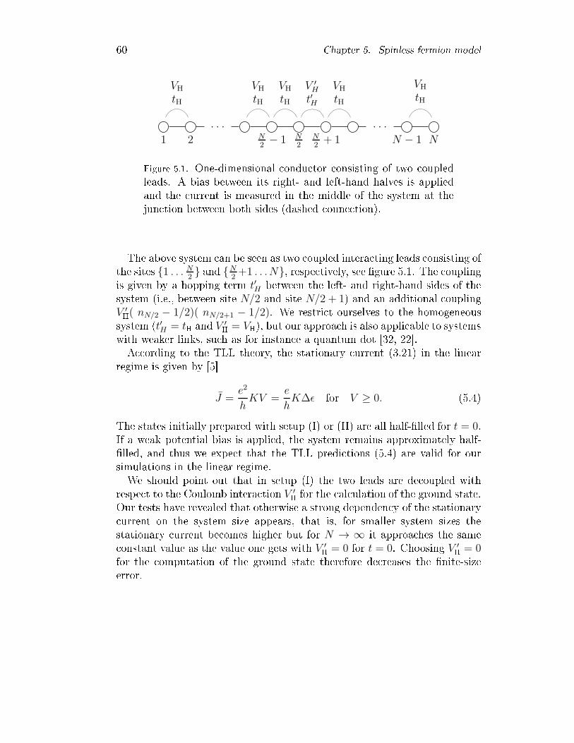
60 Chapter 5. Spinless fermion modelb b b b b b

1 2 N2− 1 N

2N2+ 1 N − 1 N

tH

VHtH

VHtH

VHt′H

V ′H

tH

VHtH

VH

Figure 5.1. One-dimensional ondu tor onsisting of two oupledleads. A bias between its right- and left-hand halves is appliedand the urrent is measured in the middle of the system at thejun tion between both sides (dashed onne tion).The above system an be seen as two oupled intera ting leads onsisting ofthe sites 1 . . . N2 and N

2+1 . . .N, respe tively, see gure 5.1. The ouplingis given by a hopping term t′H between the left- and right-hand sides of thesystem (i.e., between site N/2 and site N/2 + 1) and an additional oupling

V ′H( nN/2 − 1/2)( nN/2+1 − 1/2). We restri t ourselves to the homogeneoussystem (t′H = tH and V ′H = VH), but our approa h is also appli able to systemswith weaker links, su h as for instan e a quantum dot [32, 22.A ording to the TLL theory, the stationary urrent (3.21) in the linearregime is given by [5J =

e2

hKV =

e

hK∆ǫ for V ≥ 0. (5.4)The states initially prepared with setup (I) or (II) are all half-lled for t = 0.If a weak potential bias is applied, the system remains approximately half-lled, and thus we expe t that the TLL predi tions (5.4) are valid for oursimulations in the linear regime.We should point out that in setup (I) the two leads are de oupled withrespe t to the Coulomb intera tion V ′H for the al ulation of the ground state.Our tests have revealed that otherwise a strong dependen y of the stationary urrent on the system size appears, that is, for smaller system sizes thestationary urrent be omes higher but for N → ∞ it approa hes the same onstant value as the value one gets with V ′H = 0 for t = 0. Choosing V ′H = 0for the omputation of the ground state therefore de reases the nite-sizeerror.

5.1. Simulation parameters and errors 615.1 Simulation parameters and errorsFor the realtime simulations, we use the TEBD method des ribed in hapter 4with a maximal S hmidt dimension in the range of 300 ≤ χc ≤ 500, depend-ing on the spe i parameter ombination. We use a site-dependent χc(site)and allow our simulations to adapt χc(site) if test values (dis arded weight,entanglement entropy) show the ne essity to do so. We have to remark thatfor higher |VH| and ∆ǫ the orrelations (and thus the needed S hmidt dimen-sion) within the spinless fermion model grow very qui kly. Hen e, the hosenχc-range an lead to signi antly larger errors in the regime |VH| ≥ 1.6tH and∆ǫ ≥ 3tH.

0 10 20 30 40

10-12

10-11

10-10

10-9

10-8

Time t @ÑtH D

DN2

Figure 5.2. Dis arded weight DN/2 for dierent parameters. solidbla k urve: ∆ǫ = 0.5tH, VH = 0.8tH, dashed blue urve: ∆ǫ =tH, VH = 1.6tH, dotted red urve: ∆ǫ = 2tH, VH = 0. The verti allines indi ate the runaway times des ribed in the text.Figure 5.2 shows the dis arded weight for dierent parameters for a splitin the middle of the hain. One an see the runaway time (see hapter 4)indi ated by the verti al lines. However, the maximal dis arded weight overall simulations, sites and times up to 40~/tH we measured is yet smallerthan 10−6. Our simulations reveal that when taking a maximal S hmidtdimension of χc = 600 instead of 300, the runaway time is shifted only about20% to larger times and the quantities of interest are only slightly hanged.

62 Chapter 5. Spinless fermion modelMoreover, the stationary urrent omputed with the FABE approa h, is only hanged by less than 0.5%.We use a time step δt = 0.01, a system size N = 100 and a typi al simu-lation runs approximately 1/2 to eight hours for a ground state al ulationand about four hours to one week for a realtime evolution. We have used 12threads for a TEBD simulation on average. The total single- ore CPU timeneeded to obtain the simulation results in this hapter amounts to approxi-mately two million hours.5.2 Simulation resultsIn this se tion, we dis uss our results for the stationary urrent in the spinlessfermion model and show our ndings for the nite-system period as a fun tionof the intera tion strength VH.5.2.1 Current-voltage hara teristi s

æææ

æ

æ

æ

æ

æ

æ

æ

ààà

à

à

à

à

à

à

ììì

ìì

ìììì

òòò

òòòòòòò

ôôô

ô

ôô ô ô ô

ççççççççççççççççç

0 1 2 3 40

1

2

3

4

DΕ @tH D

J@t

He

hD

0 HeomL

1.61.20.80.40VH @tH D

Figure 5.3. Current-voltage urve of the spinless fermion modelwith setup (I) for several positive VH. For VH = 0 the urrenthas been omputed using TEBD and the one-parti le equation ofmotion (eom). The lines are guides for the eyes.In setup (I) the urrent in the non-intera ting system is proportional to∆ǫ up to the band width of the system, a ording to equation (3.22). ForVH > 0 gure 5.3 shows that the urrent in reases sub linearly with ∆ǫfor a xed intera tion strength VH and that it de reases monotoni ally with

5.2. Simulation results 63æ

æ

æ

à

à

à

ì

ì

ì

ò

ò

ò

ô

ô

ô

0.0 0.1 0.2 0.3 0.4 0.50.0

0.1

0.2

0.3

0.4

0.5

DΕ @tH D

J@t

He

hD

1.61.20.80.40VH @tH D

Figure 5.4. Magni ation of gure 5.3. The lines indi ate the linearresponse a ording to the TLL theory (5.4) for small ∆ǫ.in reasing VH for a xed potential bias ∆ǫ. The magni ation in gure 5.4shows a omparison with the linear response in the TLL theory (5.4) for small∆ǫ, using the Bethe Ansatz solution parameters (5.3). The good agreement onrms the validity of our approa h. Obviously, an in reasing VH does notonly redu e the urrent but also the range of the potential bias ∆ǫ for whi hthe linear response approximation remains valid.In gure 5.5 we observe a behaviour for attra tive intera tions VH < 0whi h is quite similar to the non-intera ting ase. The urrent in reasesalmost linearly with ∆ǫ and then saturates at a VH-dependent maximum. AsVH is in reased, the maximal urrent is de reased but also a higher linear ondu tan e is present for small applied voltages. Figure 5.6 shows that fornegative intera tions our results agree as well with the TLL theory (5.4) forsmall ∆ǫ. Again, in reasing |VH| seems to redu e the range of the potentialbias ∆ǫ for whi h the linear response approximation remains valid.We an easily understand the appearan e of the plateaus in the IV urvesfor large applied voltages. In setup (I), one half of the hain initially on-tains more parti les than the other one due to the applied potential bias ∆ǫ.When ∆ǫ is large enough to separate the system into a ompletely lled anda ompletely empty reservoir (i.e., when saturation o urs), in reasing theapplied voltage does not in rease the urrent anymore. A ording to expres-sion (3.22), this saturation o urs for non-intera ting fermions at ∆ǫ = 4tH.For an attra tive intera tion VH < 0, the parti les are more likely to sti ktogether and thus even more parti les gather in one half of the system. There-fore, saturation o urs for even smaller applied voltages, see gure 5.5. When

64 Chapter 5. Spinless fermion modelæææ

æ

æ

æ

æ

æ

æ

æ

à

àà

à

à

à

à

à à à

ì

ìì

ì

ì

ìì ì ì ì

ò

òò

ò

ò ò ò ò ò ò

ô

ô

ô

ô ô ô ô ô ô ô

ç

ççç ç ç ç ç ç ç

0 1 2 3 40

1

2

3

4

DΕ @tH D

J@t

He

hD

-1.9-1.6-1.2-0.8-0.4

0VH @tH D

Figure 5.5. Current-voltage urve of the spinless fermion modelwith setup (I) for several negative VH. The dashed lines indi- ate the theoreti al beginning of the urrent plateaus a ordingto (5.5). The solid lines are guides for the eyes.

æ

æ

æ

à

à

à

ì

ì

ì

ò

ò

ò

ô

ô

ô

0.0 0.1 0.2 0.3 0.4 0.50.0

0.2

0.4

0.6

0.8

1.0

1.2

DΕ @tH D

J@t

He

hD

-1.6-1.2-0.8-0.40

VH @tH D

Figure 5.6. Magni ation of gure 5.5. The lines indi ate the linearresponse a ording to the TLL theory (5.4) for small ∆ǫ.VH > 0, the ee t is reversed, and thus saturation o urs at higher values∆ǫ > 4tH, beyond the potential range shown in gure 5.3. The de reasing ofthe plateau heights with in reasing |VH| is not yet understood.We an approximately determine for whi h potential dieren e ∆ǫ thesystem rea hes saturation. Removing a single parti le from the ompletely

5.2. Simulation results 65lled reservoir or adding one parti le to the empty half osts an energy∆ε/2−VH − 2tH . Thus, saturation o urs if

∆ε ≥ 2VH + 4tH . (5.5)Figure 5.5 shows that this approximation ts well to the numeri al data forVH ≤ 0 whereas the saturated regime a ording to (5.5) for VH > 0 liesoutside the potential range shown in gure 5.3, as mentioned above.

æ

æ

æ

æ

æ æ

æ

æ

ææà

à

à

à

à

à

à

à

à

àì

ì

ì

ì

ì

ìì

ì

ì

ì

ò

ò

ò

ò

ò

òò ò

ò

ò

ô

ôô

ô

ô

ôô ô

ô

ô

ç

çç

ç

çççç ç

ç

ááííííííííííííííííííííííííííííííííííííííííí

0 1 2 3 40.0

0.2

0.4

0.6

0.8

1.0

1.2

DΕ @tH D

J@t

He

hD

0 HeomL

21.61.20.80.40VH @tH D

Figure 5.7. Current-voltage urve of the spinless fermion modelwith setup (II) for several positive VH. For VH = 0 the urrenthas been omputed using TEBD and the one-parti le equation ofmotion (eom). The lines are guides for the eyes.While for setup (I) the dierential ondu tan e is always positive, we ob-serve a negative dierential ondu tan e in setup (II) for VH ≥ 0, see g-ure 5.7. The urrent seems to vanish for very large potential biases as pre-di ted by strong- oupling perturbation theory for this setup. We note thatthe urrent be omes smaller with in reasing VH for a small potential bias.For larger ∆ǫ the behaviour of I as a fun tion of VH is no longer monotoni .Additionally, it an be seen that the position of the maximum of I as a fun -tion of ∆ǫ is shifted to higher values with in reasing VH. The magni ationfor small ∆ǫ (gure 5.8) onrms again that our results agree with the TLLtheory in the linear regime and that the range of the linear response regimeshrinks with in reasing intera tion strength.For setup (II) and VH < 0, gure 5.9 shows again a negative dierential ondu tan e and a vanishing urrent for very large potential biases. In on-trast to the ase VH > 0 for this setup, we see that the maximum of the

66 Chapter 5. Spinless fermion modelæ

æ

æ

à

à

à

ì

ì

ì

ò

ò

ò

ô

ô

ô

ç

ç

ç

0.0 0.1 0.2 0.3 0.4 0.50.0

0.1

0.2

0.3

0.4

0.5

DΕ @tH D

J@t

He

hD

21.61.20.80.40VH @tH D

Figure 5.8. Magni ation of gure 5.7. The lines indi ate the linearresponse a ording to the TLL theory (5.4) for small ∆ǫ.

æ

æ

æ

æ

æ æ

æ

æ

ææà

à

à

à

à

à

à

àà àì

ì

ì

ì

ì

ì

ìì ì ìò

ò

ò

ò

òò ò ò òô

ô

ô

ô

ôô ô ô

0 1 2 3 4

0.0

0.2

0.4

0.6

0.8

1.0

1.2

DΕ @tH D

J@t

He

hD

-1.6-1.2-0.8-0.40

VH @tH D

Figure 5.9. Current-voltage urve of the spinless fermion modelwith setup (II) for several negative VH. The lines are guidesfor the eyes. urrent is shifted to lower values of ∆ǫ for in reasing |VH|. Finally, the datain gure 5.10 shows the good agreement between our results and the TLLtheory predi tions in the small bias regime. We again see, that the inter-a tion strength rapidly redu es the range of potential biases for whi h thelinear response remains valid.

5.2. Simulation results 67æ

æ

æ

à

à

à

ì

ì

ì

ò

ò

ô

ô

ô

0.0 0.1 0.2 0.3 0.4 0.50.0

0.2

0.4

0.6

0.8

1.0

1.2

DΕ @tH D

J@t

He

hD

-1.6-1.2-0.8-0.40

VH @tH D

Figure 5.10. Magni ation of gure 5.9. The lines indi ate thelinear response a ording to the TLL theory (5.4) for small ∆ǫ.The negative dierential ondu tan e whi h is observed in setup (II) for allVH an be understood in terms of the overlap of the energy bands for elemen-tary ex itations. Our simulations show that there is no signi ant dieren ein the urrent urve whether one initially does or does not ouple sour e anddrain (the two halves of the system). For the following onsiderations we antherefore regard sour e and drain as initially de oupled, having two separatebut equal energy bands. Then we apply a step-like voltage in setup (II) andthus shift the two bands against ea h other. For VH = 0 only overlappingo upied one-parti le states in the sour e and uno upied ones in the drain ontribute to the urrent. While this overlap rises with in reasing |∆ǫ| from0 to 2tH, it diminishes from ∆ǫ = 2tH and rea hes zero at 4tH. As a result,the urrent is maximal for ∆ǫ ≈ 2tH and vanishes for large ∆ǫ. Similarly, we an understand the non-monotoni behaviour in intera ting ases (VH 6= 0)in terms of the overlap of the elementary ex itation bands in the spinlessLuttinger liquids in the two halves of the system. However, the ee tivebandwidth is renormalized like the Fermi velo ity in equation (5.2). There-fore, the maximum of the urrent is rea hed for a smaller potential bias ∆ǫwhen VH be omes negative as shown in gure 5.9, and shifted to a higher po-tential bias when VH is in reased, see gure 5.7. Our on lusion agrees withthe ndings in [43 where it is shown that within a similar one-dimensionalmodel a negative dierential ondu tan e is mainly aused by nite ele trodebandwidths.

68 Chapter 5. Spinless fermion model5.2.2 Inuen e of VH on the period TmaxOur results show a further ee t of VH on the nite-system urrent. Whilefor VH > 0 the period of the re tangular os illation be omes smaller, it growsfor negative intera tions.

ææ æ

æ

æ

ææ

æ

æ

ææ

æ

à

àà

à

æææææææ

æ

æ

æ

ààààààà

à

à

àSetup (I)

Setup (II)

0.0 0.2 0.4 0.6 0.8 1.0 1.20

50

100

150

200

v-1 @ÑaLtH D

Tm

ax@Ñt

HD

Figure 5.11. Period Tmax of the re tangular urrent os illation inthe nite spinless fermion model as a fun tion of the inverse renor-malized Fermi velo ity v−1 from expression (5.2). The dashedlines are des ribed by equation (5.6).Figure 5.11 shows the period Tmax of the re tangular urrent os illation inthe nite system as a fun tion of the inverse renormalized Fermi velo ity v−1from expression (5.2). The Tmax values are mean values from various ∆ǫ forea h setup. These values agree perfe tly with the dashed lines in gure 5.11whi h are given by the equationTmax(VH) = v(VH = 0)

v(VH) Tmax(VH = 0). (5.6)Thus, the period is fully determined by the time-s ale of the non-intera tingsystem Tmax(VH = 0) from (B.15) and the renormalized Fermi velo ity vfrom expression (5.2).

5.3. Summary 695.3 SummaryIn this hapter we have applied the TEBD method and our FABE approa hto obtain stationary urrent values in the full voltage range for the spinlessfermion model. We found that while in the linear regime the results aremostly independent from the spe i setup, the non-linear hara teristi sare primarily determined by it. For setup (I) the system shows a positivedierential ondu tan e over the full voltage range and the urrent satu-rates at a nite value for both, repulsive and attra tive intera tions VH. Forsetup (II) we observe a negative dierential ondu tan e and for large appliedvoltages the urrent vanishes. The ee ts from setup (II) also o ur in thenon-intera ting ase and ome from the nite bandwidth and the nonlineardispersion of the ex itations [42, 43.Finally, it turned out that the period of the os illating urrent in thenite system is fully determined by the time-s ale of the non-intera tingsystem Tmax(VH = 0) from (B.15) and the renormalized Fermi velo ity vfrom expression (5.2), a ording to equation (5.6).

70 Chapter 5. Spinless fermion model

71Chapter 6Hubbard modelSo far in this thesis we have investigated one-dimensional non-intera tingquantum systems in hapter 3 and extended this study to intera ting spinlessfermions in hapter 5. However, spinless fermions are in most ases far awayfrom a realisti des ription of ele trons in a solid. The simplest model whi h overs ele tron-ele tron intera tion for parti les with spin is the fermioni Hubbard model [66, 67, 68.This model has been under permanent resear h sin e its invention in theearly 1960s. Among others, the model was widely studied to investigateheavy fermions, the magneti properties of solids and high-temperature su-per ondu tivity. Over the years, several methods have been used to studythe Hubbard model, for instan e mean eld al ulations [69, studies us-ing perturbation theory and numeri al methods like the quantum MonteCarlo [70, 71 or the DMRG method [72.At half-lling the one-dimensional Hubbard model des ribes a Mott-insula-tor for any value of the repulsive onsite Coulomb intera tion UH > 0 while forall other llings it is a metal. This Mott-metal-insulator transition shows the ompetition between the kineti energy of the fermions and the repulsion UHof two parti les [73. At half-lling and for UH > 0, the system tries to avoiddoubly o upied states su h that ea h site is preferably o upied with a singleele tron, and harge u tuations around this state are energeti ally veryexpensive. On the ontrary, the kineti energy term in the Hamiltonian triesto delo alize the parti les into Blo h states, leading to a metal for UH = 0.The one-dimensional Hubbard model without a potential bias is exa tlysolvable with the Bethe Ansatz solution and several properties su h as thefull phase diagram and elementary ex itations are well known [74, 17, 18.For small applied voltages, the transport properties are des ribed by the TLLtheory [5, 7 and the stationary urrent in the linear regime is given by

J =2e2

hKV =

2e

hK∆ǫ. (6.1)However, the orrelation exponent K an not be obtained analyti ally, butfrom numeri al solutions of the integral equation of Lieb and Wu [75. Onegets, that while for an attra tion UH < 0 the ondu tan e in the linear

72 Chapter 6. Hubbard modelregime is in reased, it be omes smaller for a repulsive intera tion UH > 0.This behavior agrees with the hara teristi s of the urrent-voltage urves inthe spinless fermion model with respe t to VH.The Hubbard Hamiltonian for a one-dimensional latti e without a potentialbias isH0 = − tH N−1∑

σ,j=1

(c†σ,jcσ,j+1 + c†σ,j+1cσ,j)

+ UH N∑

σ,j=1

(

nσ,j −1

2

)(

nσ,j −1

2

)

+ ǫ

N∑

σ,j=1

nσ,j (6.2)where tH is the hopping amplitude, UH denotes the onsite Coulomb repulsionbetween two spins, c(†)j are the fermioni annihilation ( reation) operator forsite j and spin σ, and nσ,j = c†jcj . The reason for adding an additionalpotential oset ǫ to every site is given in se tion 6.1. We drive the systemout of equilibrium by using the previously presented setups (I) and (II) withthe HamiltonianHB =

∆ǫ

2

N/2∑

σ,j=1

nσ,j −N∑

σ,j=N/2+1

nσ,j

, (6.3)perform TEBD simulations and extra t the stationary urrent (3.21) usingthe FABE method presented in hapter 2. Sin e the Hubbard model is aninsulator for half-lling, the following simulations are performed away fromhalf-lling with a xed parti le number np, leading to a ouple of problemswhi h are des ribed below.6.1 Simulation parameters, modi ations anderrorsFor the following simulations, we use the TEBD method des ribed in hap-ter 4 with a maximal S hmidt dimension of χc = 1000. The maximal dis- arded weight over all simulations, sites and times up to 40~/tH we measuredis smaller than 10−6. For the non-intera ting ase we ompare our TEBDresults with exa tly available results from one-parti le equation of motion al ulations and nd that the out omes for the stationary urrent mat hwithin an error of less than 10−3. We use a time step δt = 0.01, a system sizeN = 100 and a typi al simulation runs approximately 2-4 weeks for a groundstate al ulation and about two months for a realtime evolution. We have

6.2. Simulation results 73used 16 threads for a TEBD simulation on average. The total single- oreCPU time needed to obtain the simulation results in this hapter amountsto approximately one and a half million hours.As already mentioned above, there is a problem in the al ulation of theground state with a xed parti le number np. Basi ally, the time evolutionof TEBD is grand anoni al, allowing any parti le number from 0 to 2Nfor the Hubbard model. To for e the system into having a spe i parti lenumber one an use an implementation of TEBD with parti le symmetry,but tests performed by Alex Cojuhovs hi showed that this is only appli ablein a regime whi h is slightly away from the lling whi h the system naturallyprefers due to the applied onsite potentials. Thus, we have introdu ed theadditional potential oset ǫ in equation (6.2) with whi h we an ontrol thepreferred total parti le number of the system. We use a Newton gradientmethod during the imaginary time evolution to adapt the potential oset,i.e. we in rease or de rease the potential oset after ea h time step, depen-dent on whether the total parti le number is urrently too low or too high.Unfortunately, this pro edure an lead to very long (up to four weeks) groundstate al ulations. It would have been easier to perform the TEBD groundstate simulations with a given (and xed) potential oset ǫ, but the a tualǫ whi h is needed to enfor e a ertain parti le number np depends on thesystem size N , on UH and on the applied potential ∆ǫ.For all following simulations, we use a lling of 0.9, i.e. 90 parti les in aHubbard model with one hundred sites, whi h is slightly below half-lling.Note that for the realtime evolution, the potential oset ǫ keeps its valuefrom the omputation of the ground state.6.2 Simulation resultsIn this se tion we show the omputed potential osets for various Coulombintera tions UH and applied potentials ∆ǫ. Furthermore, we show IV har-a teristi s for the Hubbard model for setup (I). Unfortunately, due to limited omputational resour es, the high omputational ost and re urring te hni alproblems at the RRZN, results for setup (II) are not available.6.2.1 Equilibrium onsite potentialsDue to our Newton-gradient pro edure for the imaginary time evolution, wehave obtained the potential oset ǫ for repulsive and attra tive Coulombintera tion, see gures 6.1 and 6.2.

74 Chapter 6. Hubbard modelæ æ æ æ æ æ

æà à à à à à

à

ì ì

ì

ì

ò ò

ò

ò

ôôô

ô

ô

ô

0 1 2 3 4

-3.0

-2.5

-2.0

-1.5

-1.0

-0.5

0.0

DΕ @tH D

Ε@t

HD

9

6

4

2

0

UH @tH D

Figure 6.1. Potential oset ǫ for setup (I) and positive UH. Thelines are guides for the eyes.æ æ æ æ

ææ

æà à à à

à

à

àì ì ì

ì

ì

ì

ì ò òò

ò

ò

ò

ò ô ô

ô

ô

ô

ô

ô

0 1 2 3 4

-1.5

-1.0

-0.5

0.0

DΕ @tH D

Ε@t

HD

-9

-6

-4

-2

0

UH @tH D

Figure 6.2. Potential oset ǫ for setup (I) and negative UH. Thelines are guides for the eyes.

6.2. Simulation results 75When the repulsion between the parti les is in reased, the potential oset fora onstant number of parti les is de reased as expe ted, see gure 6.1. For anattra tive Coulomb intera tion this ee t is generally reversed, but for highervoltages, the potential oset is again de reased with both an in reasing ∆ǫand an in reasing |UH|, see gure 6.2. This ee t is not yet understood.6.2.2 Current-voltage hara teristi sIn setup (I) the urrent shows a similar behavior as in the spinless fermionmodel. For small applied biases it is proportional to the bias (as predi tedby the TLL theory), but for larger voltages it saturates at a nite value,dependent on the intera tion strength |UH|. While the height of the plateauis de reased with in reasing |UH| we observe the beginning of a se ond plateaufor a repulsive intera tion, whi h an be easily understood.Sin e we simulate the system with a lling of 0.9, when ∆ǫ is in reased,there omes the point when one of the system-halves approa hes half-llingand thus this half be omes gapped for UH > 0 (the rst plateau). Only whenthe applied voltage is in reased to a value high enough to over ome the Mottgap, the number of ele trons in this half an in rease beyond one per site andthe urrent is again in reased. For still higher voltages the urrent saturatesat its a tual maximum when one half of the system has a maximal llingand the other one is empty. The position of the se ond plateau is shifted tohigher values of ∆ǫ with in reasing UH, in agreement with the in rease of theMott gap, see gure 6.3.We note that our results an not be ompared with the TLL predi tions,sin e we do not have suitable values for the small bias regime. As we knowthat for positive UH (K < 1) the linear ondu tan e should be smaller withlarger |UH|, and vi e versa for negative UH (K > 1), gures 6.3 and 6.4indi ate this behaviour.For negative UH and higher voltages in setup (I) the urrent as a fun tion oftime de ays slowly towards its stationary value. This de ay is qui k enoughfor a system of size N = 100 to obtain the stationary value from largertimes, but for times t ≈ Tmax/4 (where Tmax is the period of the re tangularos illation) this value is not yet rea hed, see gure 6.5. Our FABE approa hhas shown to be valid if we use simulation results from times t < Tmax/4,but several tests with one-parti le equation of motion out omes show thatthe method also works ne with data from times t < Tmax/2. For the resultsobtained for negative UH we have thus used data from times up to t ≈ Tmax/2where ne essary.Finally, we note that in ontrast to the spinless fermion model, the periodTmax of the nite-site re tangular os illation remains onstant for all UH.

76 Chapter 6. Hubbard model

æ

æ

æ

æ

ææ

à

à

à à à

ì

ìì ì ì

ì ì

ò

ò òò ò ò

ò

ô

ô ô ô ô ô ô

æ

æ

æ

æ

æ

à

à

à à à

ì

ìì ì ì

ì ì

ò

ò òò ò ò

ò

ô

ô ô ô ô ô ô

0 1 2 3 4 50

1

2

3

4

DΕ @tH D

J@t

He

hD

9

6

4

2

0

UH @tH D

Figure 6.3. Current-voltage urve of the Hubbard model withsetup (I) for several positive UH. For UH = 0 the urrents omputed with the one-parti le equation of motion mat h theTEBD results. The lines are guides for the eyes.

æ

æ

æ

æ

æ

æ

æ

à

à à à à à

ìì ì ì

òò ò ò ò ò

ôô ô ô ô

æ

æ

æ

æ

æ

æ

æ

à

à à à à à

ìì ì ì

òò ò ò ò ò

ôô ô ô ô

0 1 2 3 40

2

4

6

8

DΕ @tH D

J@t

He

hD

-9

-6

-4

-2

0

UH @tH D

Figure 6.4. Current-voltage urve of the Hubbard model withsetup (I) for several negative UH. The lines are guides forthe eyes.

6.3. Summary 77

DΕ=1.5, UH =-6

DΕ=4, UH =-2

DΕ=4, UH =9

0 5 10 15 20 25 30 35

0

2

4

6

Time t @ÑtH D

JHtL@t

He

hD

Figure 6.5. Currents through the middle bond in the Hubbardmodel with a system size N = 100 for setup (I) as a fun tion oftime.6.3 SummaryIn this hapter, we extended the TEBD method to be able to enfor e a xedparti le number to a system by adapting an applied potential oset. We sim-ulated the one-dimensional Hubbard model and obtained IV hara teristi sfor setup (I). Due to limited omputational resour es, the high omputational ost and re urring te hni al problems at the RRZN, results for setup (II) arenot available. Despite similar ee ts as in the spinless fermion model, wefound the beginning of a se ond plateau for positive UH. When the appliedvoltage is in reased, one half of the system rea hes half-lling and thus be- omes a Mott insulator. Only when the voltage is larger than the Mott gap,the urrent is in reased again.

78 Chapter 6. Hubbard model

79Chapter 7Two-site system oupled to a bosoni bathAs it has been argued before, latti e vibrations play an important role ina tual experimental situations, su h that we should add a bosoni bath to ourone-dimensional orrelated nanostru ture. Unfortunately, no exa t resultsor omparative data are available for the systems we investigated in thelast hapters, but sin e the TEBD method has never been used to simulatesu h systems, we have to test its appli ability rst. Therefore, we have hosen to simulate a system whi h is losely related to our problem and forwhi h omparative data from (TD) NRG [76 ((time dependent) numeri alrenormalization group) simulations are available: a two-site fermioni system oupled to a bosoni bath [44. The impurity is des ribed by the extendedHubbard model whi h ombines the nearest-neighbor Coulomb intera tionfrom the spinless fermion model and the onsite intera tion from the Hubbardmodel.At half-lling (i.e. with two parti les in the impurity), this model de-s ribes the essentials of a two-ele tron transfer in a dissipative environment.Also most investigations on su h transfer pro esses fo us on single-ele trontransfer and it has been argued that the two-ele tron transfer has a major ontribution in many pro esses, su h as in DNA [45 or in proteins [77.The original NRG method was proposed by Wilson to solve the Kondoproblem [78, 79, but re ently the method has been extended to simulatequantum impurities oupled to a bosoni bath and the realtime dynami sof systems out-of-equilibrium (see for instan e [80). While (TD) NRG pro-vides a very a urate des ription of the bosoni bath, the TEBD method anprin ipally be used to simulate even more extended impurities, su h as largemole ular bridges or nanowires. However, so far TEBD has not been usedto simulate a quantum system in a bosoni bath and it is thus important to ompare both methods to proof the appli ability of the TEBD algorithm tosu h problems.

80 Chapter 7. Two-site system oupled to a bosoni bath7.1 Two-site fermioni system in a bosoni bathWe investigate a two-site extended Hubbard model embedded in a dissipativeenvironment (bosoni bath). The rst site is alled (D)onor while the se ond

bosonic bath

|↑↓, 0〉 |0, ↑↓〉

|↑, ↓〉, |↓, ↑〉

tH tH

donor acceptor

Figure 7.1. Lo al basis of the two-site extended Hubbard model.The doubly o upied states are oupled to a bosoni bath.one is the (A) eptor, see gure 7.1. The Hamiltonian is given byH = Hel +H oupl +Hbwith the two-site operator

Hel =ǫ

2

∑

σ=↑,↓(c†DσcDσ − c†AσcAσ)− tH∑

σ

(c†DσcAσ + c†AσcDσ)

+UH(nD↑nD↓ + nA↑nA↓) +VH2

∑

σ,σ′

∑

i,j=A,D;i 6=j

niσnjσ′ (7.1)and the terms for the bosoni bath and its oupling to the two-site systemHb =

∞∑

n=1

ωnb†nbn,

H oupl =∑

σ

(nAσ − nDσ)

∞∑

n=1

λn2(b†n + bn). (7.2)

7.1. Two-site fermioni system in a bosoni bath 81The parameter ǫ des ribes an applied potential dieren e on the two fermioni sites. c(†)D,Aσ are the fermioni reation and annihilation operators for Donor(D) and A eptor (A), b(†)n are the bosoni ones and the fermioni parti lenumber operator is nD,Aσ = c†D,AσcD,Aσ. The hopping parameter is tH andthe onsite and nearest-neighbour Coulomb intera tion strength is determinedby UH and VH. The two-site extended Hubbard model (7.1) is thus an ex-tension of the normal Hubbard model by the nearest-neighbour Coulombintera tion VH whi h we already know from the spinless fermion model. It an be shown that the dynami s of the system is governed only by the dif-feren e U = UH− VH and a ordingly we will hoose VH = 0 for all followingsimulations.In all following simulations, the parti le number in the fermioni part ofthe system is set to np = 2. Thus, the lo al dimension of the two-site systemis 4 whi h is apparent from gure 7.1.7.1.1 Mapping to a semi-innite hainThe oupling term H oupl onne ts every bosoni state to the two-site system.Su h a `star' Hamiltonian annot be simulated with TEBD sin e the methodis based on the possibility to perform an alternate update of bonds whi hare not nearest neighbors. The problem of using TEBD for two-dimensionalsystems will be treated in hapter 8 in parti ular. However, the Hamiltonian an be mapped onto a semi-innite hain [81 where only the rst bosoni site ouples to the fermioni system. For the mapping we need to know thebath spe tral fun tion whi h is hosen [44J(ω) = 2παω for 0 < ω < ωc (7.3)and zero otherwise. The parameter α des ribes the oupling strength betweenthe bath and the two-site system. For simulation out omes, all variables aregiven in units of the ut-o frequen y ωc. The semi-innite Hamiltonian is

H = Hel+√η02

(b†0+b0)∑

σ=↑,↓(nAσ−nDσ)+

Nbath∑

n=0

ǫnb†nbn+

Nbath−1∑

n=0

tn(b†nbn+1+b

†n+1bn)(7.4)where ideally the length of the bosoni hain Nbath →∞ and

η0 =

∫ ωc

0

J(ω)dω =

∫ ωc

0

2παωdω = πω2cα. (7.5)Figure 7.2 shows the orresponding setup. The onsite potentials ǫn and

82 Chapter 7. Two-site system oupled to a bosoni bathǫ2ǫ0 ǫ1

α

α

tH

donor

acceptor

semi-infinite bosonic chain

t0 t1 t2 t3

ǫ3

Figure 7.2. Two-site fermioni system oupled to a semi-innitebosoni hain.hopping terms tn for the semi-innite bosoni hain from expression (7.4) an be al ulated using the following re ursion relation, whi h is initializedfor site m = 0 byU0n =

γnηs

ǫ0 =∞∑

n=0

ξnU20n

t0 =1

ηs

√√√√

∞∑

n=0

(ξn − ǫ0)2γ2n

U1n =1

t0(ξn − ǫ0)U0nwith

ηs =√η0 = ωc

√πα

γn = ηs

√

Λ2 − 1

Λ2n+2

ξn =2ωc

3

Λ3 − 1

Λn(Λ3 − Λ).

7.1. Two-site fermioni system in a bosoni bath 83The re ursion pro eeds for m > 0 asǫm =

∞∑

n=0

ξnU2mn

tm =

√√√√

∞∑

n=0

[(ξn − ǫm)Umn − tm−1Um−1,n]2

Um+1,n =1

tm[(ξn − ǫm)Umn − tm−1Um−1,n]and runs from m = 0 to Nbath − 1 to ompute the ǫm and tm for all sites.

Umn denotes an auxiliary variable and Λ is the dis retization parameter. Allthe sums whi h run to innity in lude terms ξn or γn whi h both de ayexponentially with n, wherefore we an ut the summations at a nite valueNsum = 104. Our tests have shown that a higher value Nsum = 105 does notnoti eably hange our results. Sin e even with an optimized pro edure veryhigh powers of Λ are to be al ulated, a big-integer lass [82 is needed toavoid roundo errors [83.7.1.2 General simulation parametersThe hopping term tn in (7.4) de ays exponentially with tn ∝ Λ−n, whi hnaturally allows us to take only a nite number of bosoni sites into a ount.Nevertheless, the lo al dimension mb of a bosoni site stays innite, whi hmeans that we have to ut the lo al dimension and thus allow only a nitenumber of bosons per site. For the model and parameters onsidered here, wehave used a maximal mb = 8 for the TEBD simulations, whi h orrespondsto maximally seven bosons per site.For the mapping onto a linear hain, the energy ontinuum has to be log-arithmi ally dis retized into intervals [Λ−(n+1)ωc,Λ

−nωc] with n ∈ N0 whereonly a single mode of ea h interval ouples to the impurity. This pro ess is hara terized by the dis retization parameter Λ. The dis retization is losslessfor Λ = 1 but in that ase the hopping terms tn do not de ay exponentiallywith n. Instead, a Λ > 1 has to be used whi h is small enough to give orre tresults but yet large enough su h that the hain an be ut at a su ientlysmall length Nbath. For the TEBD simulations, the length of the bosoni hain has been set to Nbath = 40 su h that the hopping term at its end issmaller than 0.02 for Λ = 1.1. We have he ked that this length is su ientfor all following simulations sin e our out omes do not noti eably hange forNbath = 30.

84 Chapter 7. Two-site system oupled to a bosoni bathApplied to the presented two-site model in a bosoni bath, the equilibriumNRG (whi h orresponds to the imaginary time-evolution for TEBD) startswith the two-site fermioni system and takes only the rst bosoni site(n = 0) into a ount. If Hn is the Hamilton operator in luding the im-purity and all sites of the bosoni system up to site n the NRG uses therenormalization group transformation to to ompute the `next' HamiltonianHn+1 whi h in ludes all bosoni sites up to n+ 1. In ea h step, only the Nslowest eigenstates of the Hamiltonian are retained. In order to give a urateresults, the NRG method needs a su iently qui k exponential de ay of thehopping terms tn su h that in every iterative step the rest of the hain on-tributes only perturbatively [84. For the following NRG simulations results,the dis retization parameter has therefore been hosen Λ = 2. Typi ally, alo al bosoni dimension mb ≥ 8 is used and Ns = 100 states are kept in ea hiteration. All NRG results presented in this thesis are based on simulationswhi h have been arried out by Sabine Tornow and whi h already have beenpublished in [44.7.2 Simulation resultsSin e the parti le number in the two fermioni sites is xed to np = 2, wedene the following observables

dD = |↑↓, 0〉〈↑↓, 0| = nD↑nD↓

dA = |0, ↑↓〉〈0, ↑↓| = nA↑nA↓

nDA = |↑, ↓〉〈↑, ↓|+ |↓, ↑〉〈↓, ↑| = nD↑nA↓ + nD↓nA↑ (7.6)whi h measure the double o upan y dD, dA of donor and a eptor and the ombined population of the singly o upied states nDA.7.2.1 Equilibrium propertiesThe equilibrium double o upan y expe tation values for ǫ = 0 in the pre-sented model have been al ulated using NRG and TEBD, see gure 7.3. Forthis symmetri model (ǫ = 0) these expe tation values are equal for donorand a eptor (in the equilibrium state)〈dD〉eq = 〈dA〉eq = 〈d〉eq. (7.7)Ea h TEBD simulation took almost one month on 8 ores. On the one hand,a very 'high' maximal S hmidt dimension χc = 150 ompared to the lo aldimension of the bosoni bath mb = 8 had to be used. We note that the

7.2. Simulation results 85U

=0

U

=Ωc

NRG

TEBDTEBD

NRG

0.0 0.2 0.4 0.6 0.80.0

0.1

0.2

0.3

0.4

0.5

Α

<d>

eq

Figure 7.3. Low-temperature equilibrium probability for doubleo upan y 〈d〉eq as a fun tion of the oupling parameter α forǫ = 0 and tH = 0.1ωc. Λ = 2 for NRG and Λ = 1.1 for TEBDwith a hain length Nbath = 40, a maximal S hmidt dimensionχc = 150 and a lo al dimension of the bath mb = 8. Note thatU = UH − VH, as des ribed in the text.simulation time of the TEBD method s ales with O(χ3

c) and O(m3b) , wherein ase of a lo al dimension of 8, a simulation performs 64 times worse thana simulation of the spinless fermion system with the same χc. This s aling an be seen in [app. C, sin e the density matrix is of size (χc ·mb)× (χc ·mb)and the main omputational time is needed to diagonalize it. On the otherhand, TEBD has never been the best andidate to al ulate the ground(equilibrium) state of a system sin e the imaginary time evolution is typi allymu h slower than for instan e the orresponding NRG or DMRG routine.Consequently, it turns out to be very hard to simulate the equilibrium stateof a system oupled to a bosoni bath using the TEBD algorithm.We note that the double o upan y 〈d〉eq de reases with in reasing U , asexpe ted, and in reases with in reasing α (see gure 7.3). For further inter-pretations see [44, where several aspe ts of the model have been investigatedin detail.

86 Chapter 7. Two-site system oupled to a bosoni bath7.2.2 Realtime dynami sFor the realtime simulations performed in this se tion, we prepare the systemsu h that initially two ele trons are lo ated in the donor and none in thea eptor. The bosoni bath is empty for t = 0. We then let the system evolvein time and the parti les start moving from donor to a eptor. The result forthe double o upan y 〈dA〉 together with the NRG simulation out omes anbe seen in gure 7.4. First, we note that our data agrees with the results from

0 100 200 300 400 500

0.0

0.2

0.4

0.6

time t @ΩcD

<d

A>HtL

Figure 7.4. Probability for double o upan y 〈dA(t)〉 as a fun tionof time for α = 0.04, ǫ = 0 (for t>0), U = −ωc and tH = 0.1ωc.Λ = 2 for NRG and Λ = 1.1 for TEBD with a hain lengthNbath = 40, a maximal S hmidt dimension χc = 150 and a lo aldimension of the bathmb = 8. The initial state has been preparedwith the two ele trons at the donor site and an empty bosoni bath. The line denotes the NRG results from [44 and the dotsare TEBD out omes for omparison.the NRG simulation. One an see a dominant os illation stemming from a oherent os illation between the two sites. It is damped, due to the ouplingto the bosoni bath, i.e. the presen e of dissipation in the impurity. As an be explained in the framework of the spin-boson model, this os illationdisappears for larger values of α leading to an overdamped urrent, see [44.In gure 7.5 we see the realtime evolution of the parti le number dis-tribution 〈nbi〉 of the bosoni bath. For t = 0 no bosons are in the bath

7.2. Simulation results 870 10 20 30 40

site i0.00

0.02

0.04

0.06

0.08

0.10

0.12

0.14

<nbiHt=0L>

0 10 20 30 40site i0.00

0.02

0.04

0.06

0.08

0.10

0.12

0.14

<nbiHt=20L>

0 10 20 30 40site i0.00

0.02

0.04

0.06

0.08

0.10

0.12

0.14

<nbiHt=80L>

0 10 20 30 40site i0.00

0.02

0.04

0.06

0.08

0.10

0.12

0.14

<nbiHt=100L>

0 10 20 30 40site i0.00

0.02

0.04

0.06

0.08

0.10

0.12

0.14

<nbiHt=130L>

0 10 20 30 40site i0.00

0.02

0.04

0.06

0.08

0.10

0.12

0.14

<nbiHt=200L>

Figure 7.5. Parti le number distribution 〈nbi〉 as a fun tion of time,in the bosoni bath for the realtime evolution with the same pa-rameters as for the simulations from gure 7.4.but as the simulation ontinues, the oupling to the impurity reates bosonswhi h start to move along the hain. A orresponding movie is available onwhypsi. om/einhellinger/bosoni BathDistribution.zip. In this movie, it be- omes more learly, that the propagation speed of the bosons is (apparentlyexponentially) redu ed over time. Thus, we found that a length of Nbath = 40is enough to simulate the time s ale depi ted in gure 7.4. Even though ingure 7.5 it looks as if the bosons had almost (in terms of time) rea hed the

88 Chapter 7. Two-site system oupled to a bosoni bathborder, this is a tually not the ase.We have performed the above simulations with various dis retizations Λ =1.1, 1.5, 1.8, 2 and found no dieren e in our out omes. Thus, we an onrmthat the simulations performed with Λ = 2 using the (TD) NRG methodmost probably reveal the true hara teristi s of the system.The TEBD simulations have been performed with a maximal S hmidt di-mension χc = 150, resulting in a maximal dis arded weight (4.13) D = 10−6.Although we have seen the appli ability of the TEBD method to systems oupled to a bosoni bath, the realtime evolution performs really badly sin ewe have to use a very small time step δt = 10−3. In ase of a Suzuki-Trotterexpansion of p-th order, the error is of the order O(δtp+1), i.e. for the se ondorder expansion (4.10) we have used, it is O(δt3). Unfortunately, TEBD isonly highly parallelizable if a high S hmidt dimension χc is needed and not asmall time step. For the simulations performed in hapter 7 only eight threads ould be used until the overhead qui kly ex eeded 10%. Thus, further eortshould be put in optimizing the TEBD algorithm for su h ases, for instan eby using a higher (for instan e fourth) order Suzuki-Trotter de ompositioneδt(F+G) = esδtF/2esδtGe(1−s)δtF/2e(1−2s)δtGe(1−s)δtF/2esδtGesδtF/2+O(δt5) (7.8)with s = 1/(2− 21/3). Using this de omposition, a one hundred times largertime step ould be applied at less than three times the omputational ostfor ea h time step. Alternatively, one ould also work on a Krylov basisusing a Lan zos diagonalization routine or with a higher order Runge-Kuttapro edure (whi h is admittedly non-unitary). Some of these solutions havealready been implemented for the td-DMRG method [85. However, thisseems to be the main task if one is interested in using the TEBD methodfor systems oupled to bosoni baths. In addition, an optimized basis forthe bosons [86, 87 ould also improve the performan e of ground state andrealtime simulations.7.3 SummaryIn this hapter, we su essfully extended the TEBD method and applied itto an impurity system oupled to a bosoni bath. We ompared our out- omes for the ground state and realtime al ulations with (TD) NRG resultsfrom [44 and found both data in good agreement. Moreover, we performedour simulations with various dis retizations Λ = 1.1, 1.5, 1.8, 2 and found nodieren e in our out omes, thus onrming that (TD) NRG al ulations with

Λ = 2 a tually give orre t results.

7.3. Summary 89Admittedly, TEBD does not perform well, neither for the ground state al ulation nor for the realtime evolution of a system oupled to a bosoni bath. An optimized basis for the bosons [86, 87 ould improve this behaviourfor imaginary and realtime evolutions, while for the realtime evolution animproved time evolution approa h seems ne essary.Nevertheless, we have proven the general appli ability of the TEBD methodto su h problems, su h that with an improved method (or using an adaptedtd-DMRG algorithm for instan e), we ould prin ipally study larger quan-tum systems oupled to phonon baths, su h as mole ular jun tions [88 ornanowires whi h are beyond rea h for the (TD) NRG method.

90 Chapter 7. Two-site system oupled to a bosoni bath

91Chapter 8Ladder systemsAs already emphasized in the introdu tion ( hapter 1), realisti nanowiresare not truly one-dimensional. Our rst step towards higher-dimensionalsystems is a ladder system, i.e. a two-dimensional model with a width ofonly a few latti e sites. Although various methods su h as the DMRG al-gorithm have been applied to study two dimensional systems [89 like thetwo-dimensional t-J-model or the Hubbard model, most resear h is on en-trated on ground state al ulations and none is on erned with the realtimedynami s of orrelated ondu tors. However, the TEBD method has notbeen used yet to study the realtime evolution of two-dimensional systemsdriven out-of-equilibrium by an external bias.Although at a rst glan e, it might seem di ult to apply TEBD to atwo-dimensional system, sin e the Suzuki-Trotter de omposition an not beused, it an be a hieved for 2D systems with a small extent in one dimension(ladder systems) by proje ting several sites onto a single one. This amountsto building an ee tively one-dimensional Hamiltonian with nearest-neighborintera tion, see gure 8.1. For every ee tive site in the new model we takethe full Hilbert spa e into a ount, i.e. given that no original sites, ea h witha lo al dimension m, ontribute to one ee tive site, the dimension of theee tive site will be mno . However, one an not simply work in the ee tivemodel as if it were one-dimensional by onstru tion, but has to keep in mindits two-dimensional origin, for instan e when omputing expe tation values.It is espe ially important to take the fermion anti- ommutation relation intoa ount.

92 Chapter 8. Ladder systems

Figure 8.1. Mapping of all sites and bonds in the smaller dimension(width) onto a single site and bond.8.1 Tight-binding ladder systemThe model whi h is hosen to show the appli ability of TEBD to two-dimensional models is des ribed by the tight-binding HamiltonianH = −tH [N−1∑

x=1

W∑

y=1

(c†xycx+1,y + c†x+1,ycxy)

+W−1∑

y=1

N∑

x=1

(c†xycx,y+1 + c†x,y+1cxy)

]

−N∑

x=1

W∑

y=1

ǫxy (8.1)where c(†)xy is the fermioni annihilation ( reation) operator for site (x, y), tHdenotes the hopping term and ǫxy is an on-site potential. Whenever onlytwo dierent potentials are applied in the system, we refer to the potentialdieren e as ∆ǫ. We study the model at half-lling. In the following, thesystem is restri ted to a width W = 2 and a length N = 60. As we want toshow the appli ability of the TEBD method to su h two-dimensional systems,we ex lude any Coulomb intera tion to be able to ompare our results withone-parti le equation of motion (3.10) out omes, sin e results for intera tingsystems are not available.8.2 Simulation parameters and errorsFor the simulations whose results are presented in the following se tion, weuse a maximal S hmidt dimension χc = 750, a system length N = 60 and atime-step δt = 0.01. Sin e the lo al dimension of the (spinless) tight-bindingmodel is m = 2, the lo al dimension of the ee tive model is m = 4, as

8.3. Simulation results 931 4 5 8 9

2 3 6 7 10Figure 8.2. Conse utive numbering of the sites in a ladder system.The bold bonds are highlighted to show the path along whi h thesites are numbered, but apart from that all bonds are equal.for instan e for the Hubbard model whi h was presented in hapter 6. One ould see the two legs in the ladder systems as the two spin hannels in theHubbard model and a ordingly the hopping from the rst to the se ond legas a spin-ip.As we are simulating fermions, it holds that due to the fermion anti om-mutation relation, a term c†jcj+n gives the phase(−1)

∑j−1i=1 ni(−1)

∑j−1+ni=1 ni = (−1)

∑j−1+ni=j ni (8.2)where ni denotes the parti le number for site i and a numbering of the sitesis ne essary, see gure 8.2. In a nearest-neighbor model in one dimension webasi ally have the terms c†jcj+1 and c†jcj . It is lear from equation (8.2) that

c†jcj has a phase 1. For c†jcj+1-terms one only gets a ontribution if thereis a parti le at the (j + 1)-site and none at site j. Thus, nj = 0, whi halso gives 1 for the phase of a nearest-neighbor hopping term. Although fora one-dimensional setup the phases an be negle ted, it is dierent for thepresented ladder system where terms c†jcj+3 with a possibly negative phaseappear, see gure 8.2. Ee tively, there is no dieren e between hard orebosons and fermions in one dimension with nearest neighbor hopping sin ewithout loops in the system, the parti les an not be inter hanged. However,this an happen in the presented fermioni ladder system.The maximal dis arded weight (4.13) for the shown simulation results issmaller than 10−8 and the maximal deviation of the TEBD results from theone-parti le equation of motion out omes amounts to a little less than 2%for the realtime evolution.8.3 Simulation resultsThe presented system is driven out of equilibrium using the two setups (I)and (II), whi h are adapted to the two-dimensional hara ter of the system.

94 Chapter 8. Ladder systemsFirst, both legs are prepared in the same way in setup (I) and (II) and the urrent JN/2,1st leg + JN/2,2nd leg through the two bonds (gure 8.3a) in themiddle is measured. Se ond, we prepare the system su h that the voltagedieren e a ording to setup (I) or setup (II) is applied between the two legs,see gure 8.3b, and the total urrent (the sum of the urrents through allbonds) from the rst to the se ond leg is measured.a) b)

leg

rungFigure 8.3. Two ways of driving the system out of equilibrium: a)All sites in the left half of the system have an applied potential+∆ǫ/2 while the rest has −∆ǫ/2, either for t = 0 (setup (I)) or fort > 0 (setup (II)). b) The same preparation, but rotated through90 degrees, i.e. rungs and legs are swit hed. The urrent is alwaysmeasured as the sum through all bonds whi h are highlighted byred arrows.The orresponding simulation results are shown in gures 8.4 and 8.5. Wenote that our TEBD results agree with the one-parti le equation of motion al ulations. However, the urrents and their stationary values are dier-ent from the results of the one-dimensional system with the orrespondingsetups. This is mostly due to a dierent ground state in whi h the parti- les are delo alized over both legs. Our simulations further show that no urrent is owing between the two legs for the simulations whose resultsare shown in gure 8.4 and a ordingly no urrent is owing between therungs in the simulations whose results are displayed in gure 8.5. We on- lude (only for the realtime evolution) that the legs (respe tively the rungs)behave like un onne ted one-dimensional stru tures for setup (I). Thus weexpe t that in an a tual experiment in luding isolated harged nanowires,many one-dimensional ee ts should be reprodu ible, although the stru -tures are not truly one-dimensional. However, further analyses of urrents intwo-dimensional systems in luding ele tron-ele tron intera tions need to bedone before we an spe ulate about a proper experimental setup.

8.4. Summary 95setup (I)

setup (II)

0 5 10 15 20 250.0

0.5

1.0

1.5

2.0

2.5

Time t @ÑtH D

JHtL@t

He

hD

Figure 8.4. Current in the ladder system prepared as shown ingure 8.3a, with ∆ǫ = 3tH and N = 60. The lines are al ulatedusing the one-parti le equation of motion (3.10) and the dotsdenote TEBD results for omparison.8.4 SummaryIn this hapter, we extended the TEBD method for two-dimensional systems,applied it to a tight-binding ladder and found that our results agree with theexa t results from the one-parti le equation of motion formalism. Further-more, our rst results indi ate that the legs (respe tively the rungs) behavelike un onne ted one-dimensional nanowires for the realtime evolution usingsetup (I).

96 Chapter 8. Ladder systems

setup (I)

setup (II)

0 1 2 3 4 5 6

-150

-100

-50

0

50

100

150

Time t @ÑtH D

JHtL@t

He

hD

Figure 8.5. Current in the ladder system prepared as shown ingure 8.3b, with ∆ǫ = 4tH and N = 60. The lines are al ulatedusing the one-parti le equation of motion (3.10) and the dotsdenote TEBD results for omparison.

97Chapter 9Summary, Con lusion & Outlook9.1 Summary & Con lusionThe goal of this thesis has been to investigate basi transport propertiesin nite and innitely large orrelated nanosystems. Additionally, we havestudied the possibilities to des ribe an a tual experimental situation better,using the time evolving blo k de imation (TEBD) method. We have startedour investigations with the lassi al LC line and investigated its transportproperties for a setup in whi h one half of the system has been initially harged. We have found explanations for many nite-size ee ts, like forinstan e the origin of the re tangular or rapid os illation, and solved themodel exa tly for the innite ase. Based on our studies we have developeda `Fourier analysis based extra tion' (FABE) method, whi h allows us toextra t the stationary urrent from out omes of analyses of nite systems.We have then shown the lose onne tion between the LC line and a quan-tum system des ribed by the tight-binding model and we implemented aone-parti le equation of motion algorithm to solve the quantum system ex-a tly. The general appli ability of our FABE approa h to quantum systemshas been rst shown in that ontext and we argued that an extrapolation ofthe stationary urrent values obtained by our approa h is unne essary if thesystem size is su iently high (N ≥ 70 in our ase).For the investigation of orrelated quantum systems su h as the spinlessfermion model or the Hubbard model, we have implemented a a multi-threaded version of the TEBD algorithm, whi h is apable of running on150 ores with an extremely low overhead. Using the TEBD method and ourFABE approa h, the full IV hara teristi s of the half-lled spinless fermionmodel and also IV hara teristi s of the Hubbard model away from half-lling have been obtained. For the Hubbard model, we have extended theTEBD method to enfor e a xed parti le number to the system by adaptingan applied potential oset during the imaginary time evolution. Thus, wehave been able to perform all simulations with the same band lling (0.9).For our simulations, we have used two dierent setups to generate a urrent.In setup (I) the initial state has dierent parti le numbers in its two halves

98 Chapter 9. Summary, Con lusion & Outlookdue to an applied potential dieren e while the system evolves in time withan overall equal onsite potential. In setup (II) we al ulate the initial statewithout a potential dieren e but turn it on for the realtime evolution.While our results for the linear regime are mostly independent from thespe i setup, the non-linear behaviour of the system is primarily determinedby it. For setup (I), we nd a positive dierential ondu tan e for the fullvoltage range and a saturation in the IV urves for higher potential biases.With setup (II) we observe a negative dierential ondu tan e that an beunderstood in terms of the overlap of the elementary ex itation bands inthe spinless Luttinger liquids in the two halves of the system. Both ee ts the plateaus and the negative dierential ondu tan e at large potentialbiases also appear in the non-intera ting ase, and are due to the nitebandwidth of the system. For the spinless fermion model, we have foundthat the period of the re tangular urrent urve in the nite system is fullydetermined by the time-s ale of the non-intera ting system Tmax(VH = 0)and the renormalized Fermi velo ity v. For the Hubbard model, a se ondplateau has been observed for positive UH whi h ould be explained in termsof the band stru ture of the model. Several omparisons (with one-parti leequation of motion results, exa t results and other numeri al data) haveshown that our methods for simulating and extra ting the stationary urrent(using TEBD and the FABE approa h) give orre t results.We have then explored the possibilities to in lude experimentally relevantextensions, su h as latti e vibrations (i.e. oupling to a bosoni bath) anda higher dimensionality of our nanostru ture. First, we have su essfullyextended the TEBD method and applied it to a two-site fermioni system oupled to a bosoni bath. Our results have been found to agree with equi-librium and realtime (TD) NRG al ulations from [44. Performing severalsimulations with dierent dis retizations Λ = 1.1, 1.5, 1.8, 2, we have foundno dieren e in the results, whi h onrms the validity of (TD) NRG al u-lations with Λ = 2. For a rst test, we have extended the TEBD method fortwo-dimensional systems and applied it to a tight-binding ladder. We foundthat our results agree with the one-parti le equation of motion al ulations,and thus we have proven that TEBD an in prin iple be use to simulate su hsystems.

9.2. Outlook 999.2 OutlookThe methods for extra ting the stationary urrent presented in this thesis an be applied to other systems, su h as systems with quantum dots or wires oupled to leads in luding ele troni and also bosoni degrees of freedom. Abosoni bath added to the drain ould for instan e hinder parti les emittedfrom sour e from being ree ted at the hard edge by taking away their kineti energy. Sin e then omputations for the urrent from a longer time-interval ould be taken into a ount, we would get more a urate results using smallersystem sizes. As we already su essfully applied the presented methods tothe spinless fermion model, the Hubbard model and a non-intera ting laddersystem, we believe that they will be very useful to study nonlinear transportproperties of orrelated low-dimensional ondu tors. We have mostly testedour approa h in the limit of transparent oupling between sour e and drain,thus it has to be he ked if the methods still work when the hybridizationbetween the leads is very small, i.e. when a weak oupling for instan ethrough a quantum dot is present.Unfortunately, we have found that TEBD performs poorly for the groundstate and realtime al ulations of bosoni systems. Using an optimized basisfor the bosons [86, 87 ould in prin iple improve this behaviour, but never-theless, an improved time evolution approa h (higher order Suzuki-Trotter,Runge-Kutta, Krylov-methods) seems to be ne essary to e iently applyTEBD to su h problems. Nevertheless, with an improved method (or anextended td-DMRG algorithm for instan e), we ould study larger quantumsystems oupled to bosoni baths, whi h are beyond rea h of the (TD) NRGmethod.

100 Chapter 9. Summary, Con lusion & Outlook

101Appendix ALC lineA.1 Current in the nite LC lineThe formal solution of equation (2.11) is given by [90

qk(t) = bk sin (ωkt) + dk cos (ωkt) (A.1)with bk, dk ∈ R given by initial onditions at time t = t0 = 0 andωk =

√

λkLC

. (A.2)The matrix mij in equation (2.12) an be analyti ally diagonalized. Usingequation (2.12), its eigenvalue equationN−1∑

j=1

mijpk,j = λkpk,i

⇒ − pk,i−1 − pk,i+1 = (λk − 2) pk,i (A.3)is solved bypk,i =

√

2

Nsin

(kiπ

N

) and λk = 2− 2 cos

(kπ

N

) (A.4)where pk,i = (~pk)i denotes the i-th omponent of the k-th eigenve tor of mijand pk,0 = pk,N = 0 was dened.Proof:sin

(kiπ

N− kπ

N

)

+ sin

(kiπ

N+kπ

N

)

= 2 cos

(kπ

N

)

sin

(kiπ

N

)

⇒ sin

(kiπ

N

)

cos

(kπ

N

)

+ cos

(kiπ

N

)

sin

(kπ

N

)

− cos

(kiπ

N

)

sin

(kπ

N

)

︸ ︷︷ ︸

=0

+ sin

(kiπ

N

)

cos

(kπ

N

)

= 2 sin

(kiπ

N

)

cos

(kπ

N

) (A.5)

102 Appendix A. LC lineUsing ~q = O−1~I from equation (2.8) and knowing that O ontains the nor-malized eigenve tors ~pk of mij in its olumns, it follows

Ii(t) =

N−1∑

k=1

pk,iqk(t) =

√

2

N

N−1∑

k=1

sin

(kiπ

N

)

qk(t) (A.6)and with the formal solution (A.1) and equation (A.6), one getsIi(t) =

√

2

N

N−1∑

k=1

sin

(kiπ

N

)

(bk sin (ωkt) + dk cos (ωkt)) (A.7)where ωk, using equations (A.2), (A.4) and cos(2x) = 1 − 2 sin2(x), is givenbyωk =

√

λkLC

=2√LC

sin

(kπ

2N

)

. (A.8)Note:Sin e O−1 = OT one an write down ck expli itlyck =

N−1∑

i=1

(O−1

)

ki

(

φi − φi+1

)

=N−1∑

i=1

pk,i

(

φi − φi+1

)

=

√

2

N

N−1∑

i=1

sin

(kiπ

N

)(

φi − φi+1

) (A.9)whi h gives us a better understanding of the ondition ck(t) = 0. Simply put,it means that φk(t) = φk+1(t) +Kk;Kk ∈ R su h that one ould for instan e`drive' the system with a homogeneous external eld and yet it would holdthat ck(t) = 0 ∀t.

A.2. Solution of the integral (2.24) 103A.2 Solution of the integral (2.24)We use the substitutions η = sin (x), a = 2t√LC

, ϕ = 2√LC

and getI∞(t) =

QL −QR√LC

1

π

∫ π2

0

sin(

2√LC

sin (x) t)

sin (x)dx

=QL −QR√

LC

1

π

∫ 1

0

sin (aη)

η√

1− η2dη

= −QL −QR√LC

1

4πaπ [−2J0(a) + πJ0(a)H1(a)− πJ1(a)H0(a)]

=(QL −QR) t

2LC[J0 (ϕt) (2− πH1 (ϕt)) + πJ1 (ϕt)H0 (ϕt)] (A.10)where Jn(x) are the Bessel fun tions of the rst kind and Hn(x) denotesthe Struve fun tion, both des ribed for instan e in [50, 91. The solutionof the integral in the se ond last transformation was found with the help ofMathemati a and an be he ked by plugging in the integral denitions ofthe mentioned fun tions.A.3 Solution of the integral (2.32)As in [app. A.2 we use the substitutions η = sin (x), a = 2t√

LC, ϕ = 2√

LCandget

Idot,∞(t) =QL −QR√

LC

1

π

∫ 1

0

sin (aη)

ηcos2(arcsin(η))

dη

dxdx

=QL −QR√

LC

1

π

∫ 1

0

sin (aη)

η(1− η2)

√

1− η2dη

=QL −QR√

LC[J1(a)

(πa

4H0(a)−

1

a2− 1

2

)

+ J0(a)

(a

2+

1

2a− πa

4H1(a)

)

]

=QL −QR√

LC[J1(ϕt)

(πϕt

4H0(ϕt)−

1

ϕ2t2− 1

2

)

+ J0(ϕt)

(ϕt

2+

1

2ϕt− πϕt

4H1(ϕt)

)

] (A.11)where Jn(x) are the Bessel fun tions of the rst kind and Hn(x) denotesthe Struve fun tion, both des ribed for instan e in [50, 91. The solution of

104 Appendix A. LC linethe integral was found with the help of Mathemati a and an be he ked byplugging in the integral denitions of the mentioned fun tions.A.4 Approximations of the Bessel and Struvefun tionsThe Bessel fun tions of the rst kind and Struve fun tions have the followingapproximations whi h be ome exa t for x→∞J0(x) =

√

2

πxcos

(

x− π

4

)

+O(1

x

)

,

J1(x) =

√

2

πxcos

(

x− 3

4π

)

+O(1

x

)

,

H0(x) =

√

2

πxsin

(

x− π

4

)

+O(1

x

)

,

H1(x) =2

π−

√

2

πxcos

(

x− π

4

)

+O(1

x

)

. (A.12)Using these expressions together with equation (2.25) leads toI l = lim

t→∞I∞(t)

= limt→∞

QL −QR

2LCt · 2ϕt

[cos2

(

ϕt− π

4

)

+ cos

(

ϕt− 3π

4

)

sin(

ϕt− π

4

)

+O(

t−32

)]

=QL −QR

2√LC

limt→∞

[cos2

(

ϕt− π

4

)

+ sin2(

ϕt− π

4

)

︸ ︷︷ ︸

1

+O(

1√t

)]. (A.13)Note that the order terms have been rewritten

O(1

t

)

→√

2

πϕtO(

1√t

) (A.14)whi h explains the unexpe ted fra tional value. One nally obtains expres-sion (2.27) for the stationary urrent whi h does not provide an approxi-mate expression for the short-time behaviour of the urrent, sin e all time-dependent terms an el out.

A.5. Remainder approximation for the Taylor series expansion 105Instead, one an use the asymptoti series expansions from [50, 92 andthe approximation of H1(x) from [51J0(x) =

(8x− 1) cos(x) + (8x+ 1) sin(x)

8√πx3

+O(

1

x52

)

,

J1(x) =(3− 8x) cos(x) + (3 + 8x) sin(x)

8√πx3

+O(

1

x52

)

,

H0(x) =8x√π(sin(x)− cos(x)) + 16

√x−√π

8π√x3

+O(

1

x52

)

,

H1(x) ≈2

π+

(16π− 5

)sin x

x

+

(12− 36

π

)(1− cos(x))

x2− J0(x) (A.15)whereas one an plug the approximate expression for J0(x) into the equationfor H1(x). Unlike J0(x),J1(x) and H0(x), the approximation of H1(x) stemsfrom [51 sin e the simple asymptoti approximation has a higher error forsmall x as shown in gure A.1. Using the given equation for H1(x) is also ru ial for an a eptable error for the approximative urrent expression (errorshown in gure A.2). Aarts and Janssen [51 state that the approximationof H1(x) has a squared approximation error on [0,∞) equal to 2.2 · 10−4 byParseval's formula but annot give a pre ise behaviour of the remainder for

x → ∞. Using the approximations (A.15), equation (2.25) for I∞(t) an betransformed into expression (2.29) for t ≫ 1. Figure A.2 shows the relativeerror between the exa t solution (2.25) and the approximation urve (2.29).A.5 Remainder approximation for the Taylorseries expansionOne an use Lagrange's remainder approximation for the Taylor series ex-pansion around zero [90, 50T [f(x)]n (x) =

n∑

i=0

f (i)(x)|x=γ

i!xi (A.16)whi h is given by

R[f(x)]n (x, γ) =

f (n+1)(x)|x=γ

(n+ 1)!xn+1 (A.17)where an upper index (n) in round bra kets denotes the n-th derivation and

γ ∈ [0, x] ⊂ R. In order to give an upper or lower border for the error, one

106 Appendix A. LC lineasymptotic series

expansion

approx. based on J0(t)

0 1 2 3 4 5

0.0

0.2

0.4

0.6

0.8

1.0

x

H1HxL

Figure A.1. Solid urve: Struve fun tion H1(x). Two approxima-tions are shown: See [93 for the expression of the asymptoti approximation (dotted line) and equation (A.15) for the approx-imation based on J0(x) (dashed line).has to hose those γ that maximize, respe tively minimize the remainder.The maximal error of an n-th order Taylor series expansion of a fun tionf(x) in the vi inity of zero is given by

En[f(x)] =maxγ(|R[f(x)]

n (x, γ)|)|f(x)| . (A.18)The approximation sin(x) ≈ x leads to R

[sin(x)]1 (x, γ) = −x2 sin(γ)/2 su hthat the maximal error for 0 ≤ x ≤ π

2is given by

E1[sin(x)] =x2

2. (A.19)

A.5. Remainder approximation for the Taylor series expansion 107

902 904 906 908 910

0.0005

0.0010

0.0015

0.0020

0 5 10 15 200.00

0.02

0.04

0.06

0.08

0.10

Time t @sD

ÈI ap

pHtL-

I ¥HtLÈÈ

I ¥HtLÈ

Figure A.2. Error ∣∣∣Iapp(t)−I∞(t)

I∞(t)

∣∣∣ with L = C = 1, QL = 1 and

QR = −1.

108 Appendix A. LC line

109Appendix BNon-equilibrium simulationsB.1 Perturbation theory for small and large bi-asesAs we hange the applied potential bias in both setups (I) and (II), theHamiltonian is a tually time-dependent and we an write it as

H(t) = H0 +∆ǫH1 · h(t) (B.1)where for setup (I) h(t) = Θ(−t) and for setup (II) h(t) = Θ(t) with Θ(0) =1. Thus, for setup (I) we initially (for times t < 0) prepare the system inthe ground state |Ψ1〉 of H0 +∆ǫH1 and the time evolution for t ≥ 0 of the(expe tation value of the) urrent is given by

J(t) = 〈Ψ1|J(t)|Ψ1〉 with J(t) = ei

~H0tJ0e

− i

~H0t. (B.2)For small applied potentials ∆ǫ, and if the ground state of H0 is not degen-erate, it holds

|Ψ1〉 = |Ψ0〉+∆ǫ · 1

H0 − E0

M1|Ψ0〉+O(∆ǫ2) (B.3)withM1 = H1 − 〈Ψ0|H1|Ψ0〉 (B.4)where |Ψ0〉 is the ground state of H0, and E0 the orresponding groundenergy. Plugging expression (B.3) into equation (B.2) one gets

J(t) = 〈Ψ0|J(t)|Ψ0〉︸ ︷︷ ︸

=〈Ψ0|J0|Ψ0〉

+∆ǫ · 〈Ψ0|(

J(t)1

H0 −E0

M1

+M11

H0 − E0

J(t)

)

|Ψ0〉+O(∆ǫ2) (B.5)

110 Appendix B. Non-equilibrium simulationsFor setup (II) the system is initially prepared in the ground state |Ψ0〉 of H0and evolved in time with H2 = H0 +∆ǫH1. Thus, it holdsJ(t) = 〈Ψ0|J(t)|Ψ0〉 with J(t) = e

i

~H2tJ0e

− i

~H2t (B.6)and using time-dependent perturbation theory

e−i

~H2t = e−

i

~H0t

(

1−∆ǫ · i~

∫ t

0

H1(t′)dt′ +O(∆ǫ2)

) (B.7)one gets after a short al ulationJ(t) = 〈Ψ0|J0|Ψ0〉+∆ǫ · 〈Ψ0|

(

(J(t)− J0)1

H0 − E0

H1

+H11

H0 − E0

(J(t)− J0))

|Ψ0〉+O(∆ǫ2) (B.8)We note that up to the order O(∆ǫ), equation (B.5) for setup (I) and equa-tion (B.5) for setup (II) are equal if 〈Ψ0|H1|Ψ0〉 = 0 and J0 ∝ [H0, H1], whi his given (or an easily be a hieved) for our models and setups.For large biases ∆ǫ and setup (II), the time evolution is determined byH = λH0 + H1. Time-dependent perturbation theory

e−i

~Ht = e−

i

~H1t

(

1− λ · i~

∫ t

0

ei

~H1t′H0e

− i

~H1t′dt′ +O(λ2)

) (B.9)yieldsJ(t) = 〈Ψ0|J(t)|Ψ0〉+ λ · i

~〈Ψ0|

∫ t

0

[H0(t′), J(t)]dt′|Ψ0〉+O(λ2) (B.10)with

J(t) = ei~H1tJ0e

− i~H1t and H0(t

′) = ei~H1t′H0e

− i~H1t′ . (B.11)Inserting (for instan e) the Hamiltonian for the spinless fermion model (5.1),one an see that the expe tation value of the urrent vanished for ∆ǫ→∞.B.2 Period of the re tangular os illation in thetight-binding modelThe following al ulation has already been performed in [94. The timeevolution of the single parti le redu ed density matrix (3.10) is given by

Gij(t) = exp

(

− i

~εqt

)

Gkq(0) exp(i

~εkt

) (B.12)

B.3. Current in the innite tight-binding model 111in the eigenbasis of a time- onstant single parti le Hamiltonian H(1). Ψk,idenotes the i-th omponent of the k-th eigenve tor of H(1) and εk the orre-sponding eigenvalue. A Fourier transformation givesGkq(ω) = δ [εk − εq − ~ω]Gkq(0). (B.13)For the tight-binding model with zero onsite potentials one hasΨk,i =

√

2

N + 1sin

(kiπ

N + 1

)

,

εk = −2tH cos

(kπ

N + 1

)

. (B.14)The period of the largest (re tangular) os illation is then given byTmax = π~

tH sin(

πN+1

) ≈ ~ · NtH for N ≫ 1. (B.15)B.3 Current in the innite tight-binding modelThe expe tation value of the urrent for setup (I) and for initial onditionslike in gure 3.4 (one ompletely lled and one ompletely empty half) is for

N →∞ given by [15, 56JkF(t) = 2etH

~

∞∑

l=k−N2

Jl(ωt)Jl+1(ωt) (B.16)where k denotes the site, ω = 2tH/~ and Jl(z) are the Bessel fun tions of therst kind. Reformulating the sum and utilizing the Bessel re ursion relation2l

zJl(z) = Jl+1(z) + Jl−1(z) (B.17)gives for z 6= 0 and k = N/2

JF(ωt) := JN/2F (ωt) =

4etH~ωt

∞∑

l=0

[(J2l+1(ωt))

2 · (2l + 1)]. (B.18)With [50

∞∑

l=0

(4l + 2ν + 2)J2l+ν+1(z)J2l+ν+1(w)

=zw

z2 − w2[zJν+1(z)Jν(w)− wJν(z)Jν+1(w)] (B.19)

112 Appendix B. Non-equilibrium simulationsfor Re(ν) > −1 and z 6= w, the urrent is given byJF(t) = 2etH

~limt′→t

ωtJ1(ωt)J0(ωt′)− ωt′J0(ωt)J1(ωt

′)

(πωt′)−1((ωt)2 − (ωt′)2). (B.20)Applying l'Hspital's rule one gets

JF(t) = etH~ωt

[(J0(ωt))

2 + (J1(ωt))2]. (B.21)

113Appendix CTEBD update s hemeIn the following part SVD and TEBDn are dened as fun tions and writtenin pseudo- ode. Let χl

c be the S hmidt dimension for site l and χlc ≤ χc ∀l.

m denotes the lo al dimension, N the number of latti e sites, i, j, k, o, p =1, 2, .., m, ξl+1 = 1, 2, .., m · χl+1

c and U l is the time evolving operator forthe l-th bond. With α = 1, 2, .., χl−1c , β = 1, 2, .., χl

c and γ = 1, 2, .., χl+1c thesingular value de omposition (SVD) is dened as:

φβ ←EW [

ρ(R)xy

]: EW [

ρ(R)xy

]> ε and β ≤ χc

Φξl+1

β ←EV [

ρ(R)xy

]ξl+1

β: EW [

ρ(R)xy

]> ε and β ≤ χc

where Φξl+1

β is the ξl+1-th omponentof the β-th eigenve torχlc ← size(φβ)

R←χlc∑

β=1

φβ (renormalization fa tor)λ[l]β ←

√

φβ/RAn eigenvalue of ρ(R) is only kept if it is larger than ε (a small numberdependent on the system) and it the maximal S hmidt dimension χc is notex eeded. A ordingly, all eigenve tors whose orresponding eigenvalues donot fulll these requirements are dis arded. We further dene TEBD1 withl = 1:

θijγ ←m∑

o,p=1

χlc∑

β=1

Γ[l]oβ λ

[l]β Γ

[l+1]pβγ λ[l+1]

γ U lopij

ρ(R)

x=j(χl+1c −1)+γ,

y=j′(χl+1c −1)+γ′

←m∑

i=1

θijγ · θ*ij′γ′ all SVD;

114 Appendix C. TEBD update s hemeΓ[l+1]jβγ ←

Φj(χl+1

c −1)+γβ

λ[l+1]γ

Γ[l]iβ ←

1

λ[l]β

·m∑

j=1

χl+1c∑

γ=1

θijγΦj(χl+1

c −1)+γβand TEBDl:

Θαijγ ←m∑

o,p=1

χlc∑

β=1

λ[l−1]α Γ

[l]oαβλ

[l]β Γ

[l+1]pβγ λ[l+1]

γ U lopij

ρ(R)

x=j(χl+1c −1)+γ,

y=j′(χl+1c −1)+γ′

←m∑

i=1

χl−1c∑

α=1

Θαijγ ·Θ*αij′γ′ all SVD;

Γ[l+1]jβγ ←

Φj(χl+1

c −1)+γβ

λ[l+1]γ

Γ[l]iαβ ←

1

λ[l−1]α λ

[l]β

·m∑

j=1

χl+1c∑

γ=1

ΘαijγΦj(χl+1

c −1)+γβand TEBDn−1 with l = n− 1:

Ωαij ←m∑

o,p=1

χlc∑

β=1

λ[l−1]α Γ

[l]oαβλ

[l]β Γ

[l+1]pβ U lop

ij

ρ(R)x=j,y=j′ ←

m∑

i=1

χl−1c∑

α=1

Ωαij · Ω*αij′ all SVD;

Γ[l+1]jβ ← Φj

β

Γ[l]iαβ ←

1

λ[l−1]α λ

[l]β

·m∑

j=1

χl+1c∑

γ=1

ΩαijΦjβfor the TEBD update s heme given in (4.12).

Bibliography 115Bibliography[1 S. Iijima, Nature 354, 56 (1991), Heli al mi rotubules of graphiti arbon[2 S. J. Tans, M. H. Devoret, H. J. Dai, A. Thess, R. E. Smalley, L. J.Geerligs, and C. Dekker, Nature 386, 474 (1997), Individual single-wall arbon nanotubes as quantum wires[3 M. Bo krath, D. H. Cobden, P. L. M Euen, N. G. Chopra, A. Zettl,A. Thess, and R. E. Smalley, S ien e 275, 1922 (1997), Single-ele trontransport in ropes of arbon nanotubes[4 S. Tomonaga, Prog. Theor. Phys. 5, 544 (1950), Remarks on Blo h'sMethod of Sound Waves applied to Many-Fermion Problems[5 T. Giamar hi, Quantum Physi s in One Dimension, Clarendon Press,Oxford (2003)[6 K. S hönhammer, J. Phys.: Condens. Matter 14, 12783 (2002), TheLuttinger liquid on ept for intera ting ele trons in one dimension[7 K. S hönhammer, in Strong Intera tions in Low Dimensions, edited byD. Baeriswyl and L. Degiorgi (Kluwer A ademi Publishers, Dordre ht,2004)[8 J. Kong, E. Yenilmez, T. W. Tombler, W. Kim, H. J. Dai, R. B. Laugh-lin, L. Liu, C. S. Jayanthi, and S. Y. Wu, Phys. Rev. Lett. 87, 106801(2001), Quantum interferen e and ballisti transmission in nanotubeele tron waveguides[9 J. N. Crain and F. J. Himpsel, Appl. Phys. A 82, 431 (2006), Low-dimensional ele troni states at sili on surfa es[10 P. S hmitte kert, Phys. Rev. B 70, 121302 (2004), Nonequilibrium ele -tron transport using the density matrix renormalization group method[11 F. Heidri h-Meisner, A.E. Feiguin, and E. Dagotto, Phys. Rev. B 79,235336 (2009), Real-time simulations of nonequilibrium transport in thesingle-impurity Anderson model[12 A. Kawabata, Rep. Prog. Phys. 70, 219 (2007), Ele tron ondu tion inone-dimension

116 Bibliography[13 A. Ya oby, in Strong Intera tions in Low Dimensions, edited by D.Baeriswyl and L. Degiorgi (Kluwer A ademi Publishers, Dordre ht,2004)[14 X. Zotos and P. Prelovsek, in Strong Intera tions in Low Dimensions,edited by D. Baeriswyl and L. Degiorgi (Kluwer A ademi Publishers,Dordre ht, 2004)[15 T. Antal, Z. Rá z, A. Rákos, and G.M. S hütz, Phys. Rev. E 59, 4912(1999), Transport in the XX hain at zero temperature: Emergen e ofat magnetization proles[16 H. Bethe, Z. Phys. 71, 205 (1931), Zur Theorie der Metalle[17 V. E. Korepin, N. M. Bogoliubov, and A. G. Izergin, Quantum InverseS attering Method and Correlation Fun tions, Cambridge Univ. Press,Cambridge (1993)[18 T. Degu hi, F. H. L. Essler, F. Göhmann, A. Klümper, V.E. Korepin,and K. Kusakabe, Phys. Rep. 331, 197 (2000), Thermodynami s andex itations of the one-dimensional Hubbard model[19 C. L. Kane and M. P. A. Fisher, Phys. Rev. Lett. 68, 1220 (1992),Transport in a one- hannel Luttinger liquid[20 A. Furusaki and N. Nagaosa, Phys. Rev. B 47, 4631 (1993), Single-barrier problem and Anderson lo alization in a one-dimensional inter-a ting ele tron system[21 G. Barak, H. Steinberg, L.N. Pfeier, K.W. West, L. Glazman, F. vonOppen, and A. Ya oby, Nature Physi s 6, 489 (2010), Intera ting ele -trons in one dimension beyond the Luttinger-liquid limit[22 E. Boulat, H. Saleur, and P. S hmitte kert, Phys. Rev. Lett. 101, 140601(2008), Twofold Advan e in the Theoreti al Understanding of Far-From-Equilibrium Properties of Intera ting Nanostru tures[23 F. Heidri h-Meisner, G.B. Martins, K.A. Al-Hassanieh, A.E. Feiguin, G.Chiappe, E.V. Anda, and E. Dagotto, Eur. J. Phys. B 67, 527 (2009),Transport through quantum dots: a ombined DMRG and embedded- luster approximation study[24 S. T. Carr, D. A. Bagrets, and P. S hmitte kert, Phys. Rev. Lett. 107,206801 (2011), Full Counting Statisti s in the Self-Dual Intera ting Res-onant Level Model[25 G. Vidal, Phys. Rev. Lett. 91, 147902 (2003), E ient Classi al Simu-lation of Slightly Entangled Quantum Computations

Bibliography 117[26 G. Vidal, Phys. Rev. Lett. 93, 040502 (2004), E ient Simulation ofOne-Dimensional Quantum Many-Body Systems[27 U. S hollwö k and S.R. White in Ee tive models for low-dimensionalstrongly orrelated systems, edited by G. G. Batrouni and D. Poilblan (AIP, New York, 2006)[28 R. M. Noa k, S.R. Manmana, S. Wessel, A. and Muramatsu, in Compu-tational Many-Parti le Physi s, edited by H. Fehske, R. S hneider, andA. Weiÿe (Springer, Berlin, 2008)[29 U. S hollwö k, Annals of Physi s 326, 96 (2011), The density-matrixrenormalization group in the age of matrix produ t states[30 A. J. Daley, C. Kollath, U. S hollwö k, and G. Vidal, J. Stat. Me h.2004, 04005 (2004), Time-dependent density-matrix renormalization-group using adaptive ee tive Hilbert spa es[31 E. Je kelmann, in Computational Many-Parti le Physi s, edited by H.Fehske, R. S hneider, and A. Weiÿe (Springer, Berlin, 2008)[32 M. A. Cazalilla and J. B. Marston, Phys. Rev. Lett. 88, 256403 (2002),Time-Dependent Density-Matrix Renormalization Group: A Systemati Method for the Study of Quantum Many-Body Out-of-Equilibrium Sys-tems[33 H. G. Luo, T. Xiang and X. Q. Wang, Phys. Rev. Lett. 91, 049701(2003), Comment on `Time-Dependent Density-Matrix RenormalizationGroup: A Systemati Method for the Study of Quantum Many-BodyOut-of-Equilibrium Systems'[34 M. A. Cazalilla and J. B. Marston, Phys. Rev. Lett. 91, 049702 (2003),Cazalilla and Marston Reply:[35 S. Kirino, T. Fujii, J. Zhao, and K. Ueda, J. Phys. So . Japan 77, 084704(2008), Time-Dependent DMRG Study on Quantum Dot under a FiniteBias Voltage[36 S. Kirino and K. Ueda, J. Phys. So . Japan 79, 093710 (2010), Nonequi-librium Current in the One Dimensional Hubbard Model at Half-Filling[37 F. Heidri h-Meisner, I. González, K.A. Al-Hassanieh, A.E. Feiguin, M.J.Rozenberg, and E. Dagotto, Phys. Rev. B 82, 205110 (2010), Nonequi-librium ele troni transport in a one-dimensional Mott insulator[38 M. nidari£, Phys. Rev. Lett. 106, 220601 (2011), Spin Transport in aOne-Dimensional Anisotropi Heisenberg Model[39 K. A. Al-Hassanieh, A. E. Feiguin, J. A. Riera, C. A. Büsser, andE. Dagotto, Phys. Rev. B 73, 195304 (2006), Adaptive time-dependent

118 Bibliographydensity-matrix renormalization-group te hnique for al ulating the on-du tan e of strongly orrelated nanostru tures[40 G. Hager, E. Je kelmann, H. Fehske, and G. Wellein, Journal of Compu-tational Physi s 194, 795 (2004), Parallelization Strategies for DensityMatrix Renormalization Group Algorithms on Shared-Memory Systems[41 P. S hmitte kert and G. S hneider in High Performan e Computing inS ien e and Engineering '06, edited by W. E. Nagel, W. Jäger, and M.Res h (Springer, Berlin, 2007)[42 A. Brans hädel, G. S hneider, and P. S hmitte kert, Annalen der Physik522, 657 (2010), Condu tan e of inhomogeneous systems: Real-time dy-nami s[43 I. Bâldea and H. Köppel, Phys. Rev. B 81, 193401 (2010), Sour es ofnegative dierential resistan e in ele tri nanotransport[44 S. Tornow, R. Bulla, F. B. Anders, and A. Nitzan, Phys. Rev. B 78,035434 (2008), Dissipative two-ele tron transfer: A numeri al renormal-ization group study[45 G. Pratviel and B. Meunier, Chem.-Eur. J. 12, 6018 (2006), Guanineoxidation: one- and two-ele tron rea tions[46 R. Hirota and K. Suzuki, Pro . IEEE 61, 1483 (1973), Theoreti al andexperimental studies of latti e solitons in nonlinear lumped networks[47 M. Toda, Physi s Reports 18, 1 (1975), Studies of a non-linear latti e[48 A. C. Singer and A. V. Oppenheim, International Journal of Bifur ationand Chaos 9, 571 (1999), Cir uit implementations of soliton systems[49 G. L. Ingold and Y. V. Nazarov, in Single Charge Tunnelling, edited byH. Grabert and M.H. Devoret (Plenum Press, New York, 1992); PreprintarXiv: ond-mat/0508728[50 A. Abramowitz and I. A. Stegun, Handbook of Mathemati al Fun tions,Dover Publi ations, New York (1972)[51 R. M. Aarts and A. J. E. M. Janssen, J. A oust. So . Am. 113, 2635(2003), Approximation of the Struve fun tion H1 o urring in impedan e al ulations[52 J. C. Slater and G. F. Koster, Physi al Review 94, 1498 (1954), Simpli-ed LCAO method for the Periodi Potential Problem[53 Y. Xue, S. Datta, and M. A. Ratner, Chem. Phys. 281, 151 (2002)First-Prin iples Based Matrix-Greens Fun tion Approa h to Mole ularEle troni Devi es: General Formalism

Bibliography 119[54 G. D. Mahan, Many-Parti le Physi s 3.Ed., Kluwer A ademi / PlenumPublishers, New York (2000)[55 E. Perfetto, G. Stefanu i, and M. Cini, Phys. Rev. Lett. 105, 156802(2010), Correlation-Indu ed Memory Ee ts in Transport Properties ofLow-Dimensional Systems[56 V. Hunyadi, Z. Rá z, and L. Sasvári, Phys. Rev. E 69, 066103 (2004),Dynami s aling of fronts in the quantum XX hain[57 D. Gobert, C. Kollath, U. S hollwö k, and G. S hütz, Phys. Rev. E71, 036102 (2005), Real-time dynami s in spin-1/2 hains with adaptivetime-dependent density matrix renormalization group[58 S. Langer, F. Heidri h-Meisner, J. Gemmer, I. P. M Cullo h, and U.S hollwö k, Phys. Rev. B 79, 214409 (2009), Real-time study of diu-sive and ballisti transport in spin- 1/2 hains using the adaptive time-dependent density matrix renormalization group method[59 N. Hatano and M. Suzuki, in Quantum Annealing and Other Optimiza-tion Methods, edited by A. Das and B. K. Chakrabarti (Springer, Berlin,2005)[60 A. Kawabata, J. Phys. So . Japan 65, 30 (1996), On the Renormaliza-tion of Condu tan e in Tomonaga-Luttinger Liquid[61 I. Sa and H. J. S hulz, Phys. Rev. B 52, 17040 (1995), Transport in aninhomogeneous intera ting one-dimensional system[62 D. L. Maslov and M. Stone, Phys. Rev. B 52, 5539 (1995), Landauer ondu tan e of Luttinger liquids with leads[63 V. V. Ponomarenko, Phys. Rev. B 52, 8666 (1995), Renormalization ofthe one-dimensional ondu tan e in the Luttinger-liquid model[64 K. Janzen, V. Meden, and K. S hönhammer, Phys. Rev. B 74, 085301(2006), Inuen e of the onta ts on the ondu tan e of intera ting quan-tum wires[65 U. S hneider, L. Ha kermüller, J. P. Ronzheimer, S. Will, S. Braun,T.Best, I. Blo k, E. Demler, S. Mandt, D. Ras h, and A. Ros h, NaturePhysi s 8, 213 (2012), Fermioni transport and out-of-equilibrium dy-nami s in a homogeneous Hubbard model with ultra old atoms[66 M. C. Gutzwiller, Phys. Rev. Lett. 10, 159 (1963), Ee t of Correlationon the Ferromagnetism of Transition Metals[67 J. Hubbard, Pro . Roy. So . London A 276, 238 (1963), Ele tron Cor-relations in Narrow Energy Bands

120 Bibliography[68 J. Kanamori, Prog. Theor. Phys. 30, 275 (1963), Ele tron Correlationand Ferromagnetism of Transition Metals[69 E. Fradkin, Field Theories of Condensed Matter Systems, Addison-Wesley, Redwood City (1991)[70 J. E. Hirs h, R. L. Sugar, D. J. S alapino, and R. Blankenbe ler, Phys.Rev. B 26, 5033 (1982), Monte Carlo simulations of one-dimensionalfermion systems[71 M. Jarrell, Phys. Rev. Lett. 69, 168 (1992), Hubbard model in innitedimensions: A quantum Monte Carlo study[72 S. Daul und R. M. Noa k, Zeits hrift für Physik B Condensed Matter103, 293 (1997), DMRG study of ferromagnetism in a one-dimensionalHubbard model[73 F. H. L. Essler, H. Frahm, F. Göhmann, A Klümper, and V. E. Ko-repin, The One Dimensional Hubbard Model, Cambridge Univ. Press,Cambridge (2005)[74 E. H. Lieb and F. Y. Wu, Phys. Rev. Lett. 20, 1445 (1968), Absen eof Mott Transition in an Exa t Solution of the Short-Range, One-BandModel in One Dimension ; Erratum: Phys. Rev. Lett. 21, 192 (1968)[75 H. J. S hulz, Phys. Rev. Lett. 64, 2831 (1990), Correlation exponentsand the metal-insulator transition in the one-dimensional Hubbard model[76 F. B. Anders and A. S hiller, Phys. Rev. Lett. 95, 196801 (2005), Real-Time Dynami s in Quantum-Impurity Systems: A Time-Dependent Nu-meri al Renormalization-Group Approa h[77 E. G. Petrov, V. I. Teslenko, and V. May, Phys. Rev. E 68, 061916(2003), Two-ele tron transfer rea tions in proteins: Bridge-mediated andproton-assisted pro esses[78 K. G. Wilson, Rev. Mod. Phys. 47, 773 (1975), The renormalizationgroup: Criti al phenomena and the Kondo problem[79 H. R. Krishna-murthy, J. W. Wilkins, and K. G. Wilson, Phys. Rev. B21, 1003 (1980), Phys. Rev. B 21, 1044 (1980), Renormalization-groupapproa h to the Anderson model of dilute magneti alloys. I. and II.Stati properties for the symmetri ase[80 F. B. Anders and A. S hiller, Phys. Rev. B 74, 245113 (2006), Spinpre ession and real-time dynami s in the Kondo model:Time-dependentnumeri al renormalization-group study

Bibliography 121[81 R. Bulla, H.-J. Lee, N.-H. Tong and M. Vojta, Phys. Rev. B 71, 045122(2005), Numeri al renormalization group for quantum impurities in abosoni bath[82 http://www.apoat.org (a big number lass) - 64bit version (v2.41)[83 W. H. Press, S. A. Teukolsky, W. T. Vetterling, and B. P. Flannery,Numeri al Re ipes: The Art of S ienti Computing, Cambridge Univ.Press, Cambridge (2007)[84 R. Bulla, T. Costi, and T. Prus hke, Rev. Mod. Phys. 80, 395 (2008),Numeri al renormalization group method for quantum impurity systems[85 A. E. Feiguin and S. R. White, Phys. Rev. B 72, 020404(R) (2005),Time-step targeting methods for real-time dynami s using the densitymatrix renormalization group[86 C. Zhang, E. Je kelmann, and S. R. White, Phys. Rev. Lett. 80, 2661(1998), Density Matrix Approa h to Lo al Hilbert Spa e Redu tion[87 C. Guo, A. Wei hselbaum, J. von Delft, and M. Vojta, Phys. Rev. Lett.108, 160401 (2012), Criti al and Strong-Coupling Phases in One- andTwo-Bath Spin-Boson Models[88 N. A. Zimbovskaya and M. R. Pederson, Phys. Rep. 509, 1 (2011),Ele tron transport through mole ular jun tions[89 E.M. Stoudenmire and Steven R. White, Annu. Rev. Condens.MatterPhys. Vol.3, 111-128 (2012), Studying Two-Dimensional Systems withthe Density Matrix Renormalization Group[90 I. N. Bronstein, K. A. Semendjajew, G. Musiol, H. Mühlig, Tas henbu hder Mathematik, Wissens haftli her Verlag Harry Deuts h, Frankfurta.M. (2008)[91 Wolfram Resear h (Mathemati a), http://mathworld.wolfram. om/[92 A. Erdélyi, Asymptoti Expansions, Dover Publi ations, New York,(1956)[93 Wolfram Resear h: http://fun tions.wolfram. om/PDF/BesselJ.pdf http://fun tions.wolfram. om/PDF/StruveH.pdf[94 M. Einhellinger, Redu ed density matrix spe tra for ele troni systemsout of equilibrium, diploma thesis, Institut für theoretis he Physik derLeibniz Universität Hannover (2007)

A knowledgmentsFirst and foremost I thank my advisor Prof. Eri Je kelmann for makingthis thesis possible, for supporting all of the ideas I ame up with and forspending a lot of time during dis ussions with me. Moreover, he always aredfor the details wedded with my thesis and my a tivities as an employee of theITP. He had shown me how to work thoroughly and a urate, publishing onlywell-proven theories and results. I always found him an inspiring example.Se ond, I thank my friends and olleagues Alex Cojuhovs hi and MartinPae h for fruitful and entertaining onversations. Even more, I would par-ti ularly like to thank Alex Cojuhovs hi for introdu ing me into the MPSand TEBD formalism (so many times), for ghting with me guratively andliterally, and for so mu h more.I also thank the NTH s hool for onta ts in nanosystems for all the edu a-tional and nan ial support. Sin ere thanks are given to Sabine Tornow andProf. Gertrud Zwi knagl from the TU Brauns hweig for the ollaborationwithin the ontext of the NTH s hool. I also thank Prof. Gertrud Zwi knaglfor agreeing to review this thesis. Spe ial thanks are given to the sta ofthe Regional Computing Center for Lower Saxony at the Leibniz UniversitätHannover (RRZN) who not only provided the omputational resour es butdedi ated themselves to serve the users to their last breaths.Eine Doktorarbeit ist so habe i h herausgefunden während vieler Phaseneine egoistis he Angelegenheit, da man kaum Zeit für die wirkli h wi htigenDinge im Leben ndet. Daher mö hte i h meiner Frau Sandra dafür danken,dass sie diese lange Zeit ertragen, mi h ertragen, mi h unterstützt, geliebt,verstanden und aufgemuntert hat. Bei meiner Mutter mö hte i h mi h dafürbedanken, dass sie mi h immer unterstützt und gefördert, für längere Zeitensehr wenig zu Gesi ht bekommen und si h nie darüber bes hwert hat. Dasglei he gilt leider au h für viele no h ni ht genannte Freunde. Dann sei no hallen ehrli h gedankt, die meinen, dass i h ihnen danken müsste, für wasimmer sie für mi h getan haben. I h war oft ni ht aufmerksam währendder Doktorarbeit, habe das vermutli h übersehen und es ni ht absi htli h alsselbstverständli h angenommen.

Curri ulum vitaeMal olm EinhellingerGeboren: 13.09.1980 in Wolfsburg (DE), dort zunä hst wohnhaft.1986 Umzug von Wolfsburg na h Tiddis he (LK Gifhorn)1987 Eins hulung in die GS Parsau1989 We hsel in die GS/OS Rühen1993 We hsel auf das Gymnasium Kreuzheide (Wolfsburg)2000 Abitur am Gymnasium Kreuzheide2001 Zvilidienst beim Paritätis hen Sozialdienst in Wolfsburg2002 Studium der Physik an der Universität Hannover,währenddessen Umzug na h Hannover2007 Diplom-Abs hluss in Physikseit 2007 Wiss. Mitarbeiter der Leibniz Universität Hannover (ITP)Wissens haftli he Publikationen:M. Einhellinger, A. Cojuhovs hi, and E. Je kelmann, Phys. Rev. B 85,235141 (2012), Numeri al method for nonlinear steady-state transport in one-dimensional orrelated ondu tors

SelbstständigkeitserklärungHiermit versi here i h, die vorliegende Dissertation selbstständig angefertigtund keine anderen als die aufgeführten Hilfsmittel und Quellen verwendet zuhaben. Keine anderen als die aufgeführten Institutionen wurden zu Hilfsleis-tungen herangezogen und keine wesentli hen Teile der Dissertation wurdenbereits als Master-, Diplom- oder ähnli he Prüfungsarbeit verwendet.____________________________Mal olm Einhellinger