range estimation using phase difference of...

UNIVERSITI TEKNOLOGI MALAYSIA

RANGE ESTIMATION USING PHASE DIFFERENCE OF ARRIVAL

TECHNIQUE

TITILOYE STEPHEN OYEDIRAN

“I hereby declare that I have read this project report and in my opinion this

project report is sufficient in terms of scope and quality for the award of the degree

of master of Engineering (Electronics & Telecommunication)”

Signature

Name of Supervisor

Date

:

:

:

………………………………………………

DR. KAMALUDIN MOHAMMAD YUSOF

31 December 2015

.

RANGE ESTIMATION USING PHASE DIFFERENCE OF ARRIVAL

TECHNIQUE

DECEMBER 2015

Faculty of Electrical Engineering

Universiti Teknologi Malaysia

A project report submitted in partial fulfillment of the

requirements for the award of the degree of

Masters of Engineering (Electronics & Telecommunication)


ii

DECLARATION

“I declare that this project report entitled “Range Estimation Using Phase

Difference of Arrival Technique” is the result of my own research except as cited

in the references. The project report has not been accepted for any degree and is

not concurrently submitted in candidature of any other degree.”

Signature

:

………………………………..

Name

:


Date

:

31 December 2015

iii

To my beloved wife, Engr. Mrs. Yetunde Titiloye – my Jewel of

inestimable value

DEDICATION

iv

Unto the Lord be the glory, great things He hath done. I praise the Almighty

God, the sustainer of my life. HIS love and mercy have seen me through this

programme. May His name be exalted for ever, Amen.

I really appreciate my project supervisor, Dr. Kamaludin Mohamad Yusof,

whose directives and academic acumen guided me properly. He’s always there for

me anytime.

My sincere heartfelt gratitude also goes to my Darling wife, Engr. Mrs.

Yetunde Titiloye and my children, Mofiyinfoluwa, Moromoluwa, Abigail, Adeola

and Nicholas for their tireless and unwavering support for me, ensuring that I

succeed all the way. I appreciate them for bearing with me and for their

understanding why I had to leave them to pursue this programme in a far country.

Thanks to Surv. Alamu E. O. of Surveying & Geoinformatics department,

Mrs. Elizabeth Gata of Business Administration department and Mrs. Buhari of

Science Laboratory department, whose financial support kick-started me on a sound

note.

I say thank you all, God bless you.

ACKNOWLEDGEMENT

v

The principle of positioning is a technology of identification that enables

object, people and/or assets to be tracked. This is basically to allow objects to be

found for the purpose of rendering/obtaining services. Ranging technique therefore

is an important part in anchor nodes location vis-à-vis the distance between anchors

to the blind node. Integration of location capability into Wireless Sensor Network

provides enablement in the location of network devices anywhere in the area of

deployment, thereby making the network more valuable from the point of view of the

application. Currently, there are several techniques which have been used to

estimate ranges, most of the approaches which are dependent on a single frequency

technique and those techniques are inaccurate in estimating the range, particularly in

a multipath environment. The proposed work was to employ a dual-frequency phase

difference of arrival technique for one-way propagation to capture ranges. Phase

Difference of Arrival technique is a dual-frequency technique of ranging that offers

better solution than already available single frequency ranging techniques. The

technique has previously been used for radar application. Having evaluated the

performance of this new technique for different frequency pairs with different

frequency separation in different noise variance level, proof of the concept is

provided using simulated data. The obtained results show that the proposed dual-

frequency Phase-Difference of Arrival system is able to correctly find the location of,

and track objects. Ranging simulation results show that frequency separation of

50MHz is best suited for one-way short-range application.

ABSTRACT

vi

Prinsip penglokasian adalah teknologi pengesanan yang membolehkan objek,

orang dan asset dikesan. Ini pada asanya membolehkan objek dikesan untuk tujuan

tindakan selanjutnya. Oleh yang demikian, teknik pengukuran jarak memainkan

peranan penting dalam menganggarkan lokasi nod melalui pengukuran jarak di

antara nod dan juga nod lain. Integrasi keupayaan penglokasian ke rangkaian

pengesan wayarles membolehkan lokasi peranti rangkaian di mana-mana dalam

penggunaan, membuat rangkaian lebih bermakna dari sudut applikasi. Pada masa

ini, terdapat beberapa teknik yang telah digunakan untuk menganggarkan jarak,

kebanyakan teknik yang sedia ada bergantung kepada teknik frekuensi tunggal dan

itu adalah kurang tepat dalam menganggarkan jarak, terutamanya dalam persekitaran

pelbagai jarak. Projek yang dicadangkan adalah dengan menggunakan teknik

perbezaan fasa ketibaan dua frekuensi bagi pergerakan isyarat sehala. Teknik

perbezaan fasa ketibaan dua frekuensi adalah teknik peanggaran jarak dwi-frekuensi

yang menjanjikan penyelesaian yang lebih baik daripada teknik-teknik yang

menggunakan frekuensi tunggal yang sedia ada. Teknik ini telah digunakan untuk

aplikasi radar. Prestasi teknik ini dinilai dari segi pelbagai kombinasi frekuensi dan

pelbagai kombinasi jarak pemisahan frekuensi di dalam keadaan pelbagai tahap

gangguan isyarat dan ia dapat dibuktikan dengan menggunakan data simulasi. Hasil

kajian menunjukkan bahawa cadangan teknik perbezaan fasa ketibaan dua frekuensi

mampu untuk meanggarkan lokasi dan mengesan objek dengan betul. Hasil kajian

menunjukkan bahawa jarak pemisahan frekuensi kurang daripada 50MHz adalah

paling sesuai untuk aplikasi jarak dekat isyarat satu hala.

ABSTRAK

vii

TABLE OF CONTENTS

CHAPTER

TITLE PAGE

DECLARATION ii

DEDICATION iii

ACKNOWLEDGEMENT iiv

ABSTRACT v

ABSTRAK vi

TABLE OF CONTENTS vii

LIST OF TABLES x

LIST OF FIGURES xi

LIST OF ABBREVATIONS xiii

LIST OF APPENDICES xv

1 INTRODUCTION 1

1.1 Introduction of the Research 1

1.2 Statement of the Problem 3

1.3 Objectives of the Study 4

1.4 Scope of the Study 5

1.5 Significance of the Study 5

1.5.1 Why Range Estimation? 6

1.5.2 Contribution of the Research to Knowledge 7

viii

1.6 Organization of the Thesis 7

2 LITERATURE REVIEW 9

2.1 Overview 9

2.2 Signal Propagation 10

2.2.1 Free-space Model 11

2.2.2 Two-ray Model 14

2.2.3 Log-normal Shadowing Model 16

2.3 Ranging Techniques 18

2.3.1 Time of Arrival 18

2.3.2 Time Difference of Arrival 20

2.3.3 Angle of Arrival 21

2.3.4 Received Signal Strength Indication 25

2.3.5 Radio Interferometric Positioning System 28

2.3.6 Swept Frequency technique 29

2.4 The Proposed Technique 29

2.4.1 The principle of operation of Radar 30

2.4.2 Range estimation based on Dual-frequency signaling 32

3 METHODOLOGY 37

3.1 Introduction 37

3.2 Tools of Research 39

3.2.1 Matlab 39

3.2.2 Universal Software Radio Peripheral 40

3.3 Possible obstacles to localization accuracy 44

ix

4 SIMULATION RESULTS AND ANALYSIS 45

4.1 Simulation Set-up 45

4.2 Propagation models simulation results 48

4.3 Range ambiguity 49

4.4 Effect of Phase Noise 51

4.5 Error Analysis 55

5 CONCLUSION 57

5.1 Introduction 57

5.2 Conclusion 57

5.3 Recommendation for Future work 58

REFERENCES 61

Appendices 67

x

LIST OF TABLES

TABLE NO.

TITLE PAGE

4.1 The operating frequencies used for Simulation 46

4.2 Distance error Vs Phase error 55

xi

LIST OF FIGURES

FIGURE NO.

TITLE PAGE

1.1 Basic Tx-Rx signal transmission 3

2.1 Signal Propagation via Free Soace Model 12

2.2 Signal Propagation via Two-Ray Model 14

2.3 Principle of Time of Arrival 18

2.4 Principle of location in Angle of Arrival Technique 22

2.5 Estimating range using Angle of Arrival 23

2.6 Trilateration approach of range estimation 26

2.7 Basic node formulation in Trilateration 27

2.8 Transmission of dual-frequency from a reader to an

object 33

2.9 Phase difference Vs Range estimate 36

3.1 Flowchart describing the project schedule 39

3.2 Universal Software Radio Peripheral 42

3.3 Experimental set-up of USRP 40

4.1 Phase difference Vs. Distance relation 47

4.2 Dual frequency Estimator results 48

4.3 Propagation Models graphs 49

4.4 Range ambiguity analysis 51

4.5 Phase difference of two signals with time 52

4.6 Effect of phase noise on the signal propagation 53

xii

4.7 Phase difference over 500 meters 55

4.8 Distance error Vs Phase error graph 56

xiii

LIST OF ABBREVATIONS

AoA - Angle of Arrival

BFDM - Biorthogonal Frequency Division Multiplexing

BS - Base Station

CW - Carrier Wave

dB - Decibel

DDC - Digtal Down Counter

DUC - Digital Up Counter

EM - Electromagnetic

f - Frequency

FFT - Fast Fourier Transform

FPGA - Field Programmable Gate Array

GE - Emitter Gate

GR - Receiver Gate

GHz - Gigahertz

I/O - Input/Output

Laser - Light Amplification by Simulated Emission of Radiation

LOS - Line of Sight

LS - Least Squares

MATLAB - MATrix LABoratory

MHz - Megahertz

MIMO - Multiple-Input, Multiple-Output

xiv

MS - Mobile Station

OFDM - Orthigonal Frequency Division Multiplexing

OQAM

- Offset Quadrature Amplitude Modulation

QAM - Quadrature Amplitude Modulation

RF - Radio Frequency

Rx - Receiver

RFID - Radio Frequency Identification

RIPS - Radio Interferometric Positioning System

RSSI - Received Signal Strength Indication

RTLS - Real Time Locating System

SI - Spherical Interpolation

SNR - Signal-to-Noise Ratio

SOI - Signal of Interest

TDoA - Time Difference of Arrival

ToA - Time of Arrival

Tx - Transmitter

USRP - Universal Software Radio Peripheral

WSN - Wireless Sensor Network

xv

LIST OF APPENDICES

APPENDIX

TITLE PAGE

A Range versus Phase-difference code 65

B Code for the effect of noise on signal propagation 66

C Distance error versus Phase error code 69

CHAPTER 1

INTRODUCTION

1.1 Introduction of the Research

Ranges of unknown node with respect to several known nodes are required in

locating the position of the unknown node. Currently, there are several techniques

which have been used to estimate ranges, such as Time of Arrival (ToA), Time

Difference of Arrival (TDoA), Angle of Arrival (AoA), Received Signal Strength

Indication (RSSI) [1], Radio Interferometric Positioning System (RIPS), and others,

described in the literature review. Most of the approaches are dependent on a single

frequency technique and those techniques are inaccurate in estimating the range,

particularly in a multipath environment.

Going by technological advances, it is observed that wireless networking

technology has been experiencing a tremendous growth and widespread adoption in

Communications Engineering. Integration of location capability into the Wireless

Sensor Network (WSN) can aid the location of network devices anywhere in the area

of deployment, making the network more valuable from the application point of

view. A Wireless Sensor Network refers to a group of sensors, or nodes that are

linked by a wireless medium to perform distributed sensing tasks. Connections

between nodes are formed using such media as infrared devices or radios. Wireless

sensor networks are usually used for such tasks as surveillance, widespread

environmental sampling, security and health monitoring. They can be used in

2

virtually any environment, even those where wired connections are not possible,

where the terrain is inhospitable, or where physical placement is difficult.

Radiolocation is achieved by measuring one or more characteristics of the radio

signal such as Received Signal Strength Indication, and Time-of-Arrival. Using

these measurements, the ranges between devices in the network are estimated and the

locations of the devices are computed based on the estimated nodes information [2].

The importance of localization which involves

(i) ranging,

(ii) positioning and

(iii) error optimization

has been applied in numerous modern applications such as personal and public

security, healthcare and military [3]. This clearly shows the importance of Range

estimation, to accurately find the location of the position of a blind or unknown node

(i.e, a sensor node in an unknown position) such as an object, person, product, asset

or vehicle.

Furthermore, crucial aspect of WSN operation produces low power

consumption [2]. There is in recognition of the fact that multi-hop communication

(messages are relayed by intermediate nodes) has the ability to improve energy

efficiency by reducing the communication range required to convey information

from a source to a destination [2]. While reducing range is attractive from power

3

consumption standpoint, the effect of communication range on range estimation and

location estimation accuracy is still being exploited [2].

There has been the usage of distance estimation using phase measurement in

many areas of Science and Engineering [3]. Particularly in this work, two signals

with different frequencies will be transmitted from the transmitter to a receiver. The

signals will arrive at the receiver at different phases. The corresponding phase

difference from these two transmitted signals will be processed to evaluate the

distance between the transmitting and receiving nodes [3]. This concept is illustrated

in Figure 1.1.

Figure 1.1 Basic Tx-Rx signal transmission

1.2 Statement of the Problem

Due to the inaccuracy which the single frequency technique poses especially

when transmitted signals are highly faded at some frequencies, it has become

necessary to employ dual frequencies to estimate the required range. This involves

transmitting signals using two different frequencies to an unknown node. This is

necessary because if one signal is transmitted, there is every tendency that it will fade

at some point along the line. This will certainly affect the outcome of the range

4

estimate carried out with it. By employing dual-frequency, obviously, the two

signals would not fade out at the same time. Even one fades, the other will be be

available to complete the task. The signals, thereby, arrive at the node at different

phases. The difference in the phases of the arriving signals would then be used to

adequately locate and estimate the node. Therefore, the problem statement for this

research is stated as follows: “How to provide frequency diversity for robust range

estimation in a wireless communication environment”.

1.3 Objectives of the Study

The task of performing this project work necessitated some objectives to be

realized. The following are therefore the objectives set out for this research work:

(i) To study the signal propagation in short-range communication,

(ii) To simulate range estimation using Phase Difference of Arrival (PDoA)

technique,

(iii) To analyze the range estimation through range ambiguity, effect of noise,

and error analysis.

5

1.4 Scope of the Study

The scope of this work is; Investigating range estimation using dual-

frequency technique, in order to find an acceptable and best-suited frequency

separation for a short-range one-way propagation scenario.

1.5 Significance of the Study

Location estimation from range measurements can he viewed as an error

minimization approach, for which Least squares (LS) is a classic approach.

However, there are aspects of the problem which, when hypothesized, could allow

better results than the LS method with the same multipath ToA datasets. First, the

ToA error (hence range error) due to multipath can only be positive. A negative

range error would imply superluminal propagation. Therefore, in any physically

consistent set of range measurements, it is impossible for the true location to lie

outside of any of the circles of measured range radii about the respective base-

stations. It is easily demonstrated that LS solutions are not consistent with this

physical principle.

Secondly, by studying the location estimates of a human presented with a

graphical representation of the base-station map and overlaid circles from sets of

ranging estimates (to known), it could be found that the best estimates tend to be

based on a visually apparent subset of range circles which tend to the most self-

consistent in terms of nearly describing a point intersection. This is rather different

to LS in which the most outlying range circles actually have more than a proportional

influence on the solution. One could weight each range measurement in an LS

6

formulation, hut this would require ancillary means to assign reliability estimates to

each range measurement. In view of the above therefore;

(1) Range-based localization of object is able to provide adequate precision as it

exploits measurements of physical quantities related to signals travelling

between the anchor and the object [4].

(2) Through range-estimation over dual-frequency pairs, the effect of noise can

be greatly reduced in the communication environment.

(3) By using range-based approach therefore, error minimization is adequately

guaranteed [5].

Hence, we can look at this sub-topic under the following sub-divisions:

1.5.1 Why Range Estimation?

In wireless communication technology, there is a rapid development of the

need for identification, location and tracking of objects such as products, assets, and

personnel, electronically. It has become one of the primarily means to construct a

Real-Time Locating System (RTLS) that tracks and identifies the location of objects

in real time.

Interestingly, there exists a relationship between range-estimates and:

(1) Bandwidth, whereby precision increases with bandwidth, but carries

diminishing returns with the additional expense;

(2) center frequency, whereby lower frequencies penetrate materials better

(where there is a building between the transmitter and the receiver).

7

The technique employed in this work, has the potential of estimating the

position of an unknown node accurately, provided that the distances between two or

more known nodes to the unknown node are well known. Hence, to have high

accuracy in positioning, the need of a robust ranging technique is required [3].

1.5.2 Contribution of the Research to Knowledge

With the single-frequency technique, when the transmitted signal is severely

faded, the technique will likely produce phase that is unreliable, and subsequently,

yield unreliable range estimation from the received signal. The employed dual-

frequency technique has the capability of taking care of this problem. Also, noise

has a greater effect on single-frequency signal, which the dual-frequency technique is

able to minimize to the barest level.

1.6 Organization of the Thesis

The field of Signal Processing has grown enormously in the past few decades

to encompass and provide firm theoretical background for a large number of

individual areas. Since range estimation, for the most part, relies on the theory of

Signal processing, it is shown as a major unifying influence for the entire work.

8

Chapter 1 introduces the general concept of the research work, providing the

statement of the problem, the objectives and the significance of the study.

Chapter 2 extensively discusses the literature review, reviewing the previous

work done in recent times on the topic and then, reviewing the related topics.

Chapter 3 dwells on the methodology of the research, including the tools

employed in carrying out the research.

Chapter 4 presents the simulation results and the analysis.

Chapter 5 is the conclusion of this report.

9

CHAPTER 2

LITERATURE REVIEW

2.1 Overview

Ranging is a phenomenon used widely for the purpose of identifying and

localizing objects electronically. It is able to offer substantial advantages for

businesses, thereby allowing automatic inventory and tracking on the supply chain.

This new technology plays a key role in pervasive networks and services. Indeed,

data can be stored and remotely retrieved through ranging, thereby enabling real-time

identification of devices and users. The functionality of ranging technology also

finds application the area of indoor navigation, precise real-time inventory, and in

library management to retrieve persons or objects, control access, and monitor events

[6].

For Range-free techniques, the actual distance measurements are not required

since the connectivity or any information available such as hop-count can be used as

estimate distance for positioning estimation. The examples of Range-free techniques

are proximity-based localization, one-hop localization and multi-hop localization [3].

10

However, Range-based localization approach get more attention in research field

since positioning is more accurate when compared to Range-free approach [3].

Range estimation, which uses single frequency, suffers from large range

uncertainty and ambiguity [7]. This is because such estimation based on a single

frequency f, has infinite range estimate solution, separated just by only half of the

corresponding wavelength [7]. This is explained well in section 2.3.1. Drastic

reduction in range ambiguity can be achieved in two ways. One is by lowering the

transmitted signal frequency so as to increase the distance between two possible

consecutive range estimates, thereby ruling out those range estimates inconsistent

with the nature of the scene [7]. Secondly, the reduction in range ambiguity is also

possible through increase in distance, making it larger than the difference between

the lower and the upper bounds on target location [7]. However, the range ambiguity

can be totally eliminated by employing dual-frequency pairs in the transmission of

signals from the transmitter to the receiver [8].

2.2 Signal Propagation

Basically, there are two ways of transmitting an electro-magnetic (EM)

signal, namely either through a guided medium or through an unguided medium.

Guided mediums such as coaxial cables and fiber-optic cables are far less hostile

toward the information carrying EM signal than the wireless or the unguided

medium. It presents challenges and conditions which are unique for this kind of

transmissions [9]. As s signal travels through the wireless channel, it undergoes

many kinds of propagation effects such as reflection, diffraction and scattering. This,

of course is due to the presence of buildings, mountains and other such obstructions.

11

Reflection occurs when the EM waves impinge on objects which are much greater

than the wavelength of the traveling wave. Diffraction is a phenomena occurring

when the wave interacts with a surface having sharp irregularities. Scattering occurs

when the medium through the wave is traveling contains objects which are much

smaller than the wavelength of the EM wave.

These varied phenomena’s lead to large scale and small scale propagation

losses. Due to the inherent randomness associated with such channels they are best

described with the help of statistical models. Models which predict the mean signal

strength for arbitrary transmitter receiver distances are termed as large scale

propagation models. These are termed so because they predict the average signal

strength for large Tx-Rx separations, typically for hundreds of kilometers.

Further analysis was carried out with the signal propagation via the following

models:

2.2.1 Free-space Model

Generally, EM signals when traveling through wireless channels, usually

experience fading effects due to various effects, but in some cases the transmission is

with a direct line of sight such as is obtained in satellite communication. Free space

model, depicted in Figure 2.1 predicts that the received power decays as negative

square root of the distance.

12

Figure 2.1 Signal propagation via Free-space model

Friis free space equation is given by,

Ld

GGPdP rttr 22

2

)4()(

πλ

= (2.1)

where Pt is the transmitted power,

Pr(d) is the received power,

Gt is the transmitter antenna gain,

Gr is the receiver antenna gain,

λ is a factor which depends on the propagation environment,

d is the Tx-Rx separation and

L is the system loss factor which depends upon line attenuation, filter losses

and antenna losses and not related to propagation.

The gain of the antenna is related to the effective aperture of the antenna

which in turn is dependent upon the physical size of the antenna given as follows:

2

4λπ eAG = (2.2)

where Ae = effective aperture of the antenna.

13

The path loss, which represents the attenuation suffered by the signal as it

travels through the wireless channel is given by the difference of the transmitted and

received power in dB and is expressed as:

=

r

t

PPdBPL log10)( (2.3)

The fields of an antenna can be classified in two broad regions, namely the

far field and the near field. It is in the far field that the propagating waves act as

plane waves and the power decays inversely with distance. The far field region is

also termed as Fraunhofer region and the Friis equation holds in this region. Hence,

the Friis equation is used only beyond the far field distance, df, which is dependent

upon the largest dimension of the antenna as:

λ

22Dd f = (2.4)

where df = far-field distance, and

D is the largest dimension of the antenna.

Also we can see that the Friis equation is not defined for d = 0. For this

reason, we use a close in distance, do, as a reference point. The power received,

Pr(d), is then given by:

2

00 )()(

=

dddPdP rr (2.5)

14

The major drawback in this technique is that the RSSI-based systems usually

need on-site adaptation in order to reduce the severe effects of multipath fading and

shadowing in indoor environments [10].

2.2.2 Two-ray Model

Two-ray model is also known as Ground Reflection model. It is a simple

model for propagation over ground, pictorially represented as shown in Figure 2.2.

Figure 2.2 Signal propagation via Two-ray model

Here, two components of transmitted signals arrive at the receiver – one LOS

and the other reflected from the ground. For small angle of incidence, it is assumed

that the reflection coefficient, 1−=Γ .

15

At large distances compared to the antenna heights the two components will

have approximately equal amplitude and a small phase difference given by:

λπδθδ

2= (2.6)

where dhh rt2

≈δ .

For large (d » )rt hh , it can be shown that the received power is,

4

22

dhhGGPP rt

rttr = (2.7)

where Pt = transmitted power,

Gt = gain of the transmitter,

Gr = gain of the receiver,

ht = height of the transmitter above ground level,

hr = height of the receiver above ground level, and

d = distance between the transmitter and the receiver.

16

For this model, the path loss varies as d4, the square of the antenna height and

is independent of the frequency [2].

2.2.3 Log-normal Shadowing Model

In radio communications, the levels of the received signal usually decrease as

the distance between the transmitter and the receiver increases. This phenomenon is

known as path-loss. Attenuation of radio signals due to the path-loss effect has been

modeled by averaging the measured signal powers over long times and over many

distances around the transmitter. The averaged power at any given distance to the

transmitter is referred to as the area mean power Pa (in Watts or milli-Watts). The

path-loss model states that Pa is a decreasing function of distance r between

transmitter and the receiver and can be represented by a power law:

η−

=

0

)(rrcrPa (2.8)

where Pa = power received at the receiver,

c = velocity of electromagnetic wave,

r = distance between transmitter and receiver, and

r0 = reference distance.

17

In Equation (2.8), r0 is a reference distance. Parameter η is the path-loss

exponent which depends on the environment and terrain structure and can vary

between 2 in free space to 6in heavily built urban areas. The constant c depends on

the transmitted power, the receiver and the transmitter antenna gains and the

wavelength. The path-loss model is often used in the study of wireless ad-hoc

networks. However, this model could be inaccurate because in reality, the received

power levels may show significant variations around the area mean power. This

model is the log-normal shadowing model, and allows for random power variations

around the area mean power. Let the received power at distance r from the

transmitter be denoted by P(r). In the log-normal shadowing model the basic

assumption is that the logarithm of P(r) is normally distributed around the

logarithmic value of the area mean power [11]:

xrPrP a += ))((log10))((log10 1010 (2.9)

In Equation (2.9), x is a zero-mean normal distributed random variable (in

dB) with standard deviation σ (also in dB). The standard deviation is larger than zero

and, in some special cases where there are severe signal fluctuations due to

irregularities in the surroundings of the receiving and transmitting antennas, it can be

as high as 12 [12]. It could be noticed that if σ is assumed to be equal to zero, the

log-normal model will be the same as the path-loss model. So, the path-loss model

can be seen as a specific case of the more general log-normal model.

18

2.3 Ranging Techniques

Work has been carried out in the area of estimating ranges of some objects

using various techniques. While many techniques employ single-frequency, few

other techniques employ dual-frequency. Some of these techniques are hereby

discussed, in terms of their modes of operation. Their drawbacks and shortcomings

are clearly stated.

2.3.1 Time of Arrival

In the Time of Arrival (ToA) technique, the one-way propagation time of the

signal traveling between a mobile station (MS) and each of the base stations (BSs) is

measured, and this provides a circle centered at the BS on which the MS must lie.

The ToA measurements are then converted into a set of circular equations, from

which the MS position can be determined with the knowledge of the BS geometry.

Figure 2.3 shows the diagrammatic representation of the principle behind ToA.

Figure 2.3 Principle of Time of Arrival

19

Basically, what is needed here is to estimate the range (distance) between the

Transmitter (Tx) and the Receiver (Rx). And this is done by sending the signal from

the transmitter and then taking note of the time it takes the signal to arrive at the

receiver. Then, the required estimation is carried out using:

tXctR =)( (2.10)

where R(t) is the required range,

c is the velocity of electromagnetic wave, and

t is the time of travel for the signal.

A straightforward approach for determining the MS position is to solve the

nonlinear equations relating these measurements directly, but it is computationally

intensive [13]. Apart from the direct methodology, another common technique that

avoids solving the nonlinear equations is to linearize them, and then, the solution is

found iteratively. However, this latter approach requires an initial estimate and

cannot guarantee convergence to the correct solution unless the initial guess is close

to it.

To allow real-time implementation and ensure global optimization, the idea

of the spherical interpolation (SI) in Time Difference of Arrival (TDoA)-based

location is adopted. Here, the nonlinear hyperbolic equations are reorganized into a

set of linear equations by introducing an intermediate variable, which is a function of

the source position. However, the SI estimator solves the linear equations directly

20

via least squares (LS) without using the known relation between the intermediate

variable and the position coordinate.

In ToA technique of estimating range, the distance between a reference point

and the target is proportional to the propagation time of signal. ToA-based systems

need at least three different measuring units to perform adequate positioning in 2-D.

This is a major drawback of this technique. Moreso, the technique also requires that

all transmitters and receivers are precisely synchronized so that the receiver can

know when the transmitter starts sending the signal.

2.3.2 Time Difference of Arrival

With the Time Difference of Arrival (TDoA) technique, two observing

antennas are held a fixed distance from each other. These distances are typically

large. Receivers with pre-detection outputs are then attached to the two antennas,

and the two resultant outputs are cross-correlated. The peak output from the cross-

correlation is a measure of the TDoA between the observation points. A line of

position may be calculated from the cross-correlation peak. In the case of a wide-

band signal of interest (SOI) in an environment of narrow-band interference, the

determination of the cross-correlation peak is extremely difficult and often

impossible due to equipment limitations. This is particularly true if the interference

is of smaller bandwidth than the SOI. Such interference then has a broad cross-

correlation function which typically obscures the correlation function of the SOI

[14].

21

TDoA is very much related to ToA in the sense that both employ single

frequency. The only difference is that in TDoA, the single frequency are sent out

from the transmitter tow times, taking proper note of the time that the signals were

sent. This is necessary in order to use the difference in time of the arrivals of the

signals for the purpose of estimating the required range. The principle of TDoA lies

on the principle of determining the relative location of a targeted transmitter by

employing the difference in time at which the signal emitted by a target arrives at

multiple measuring units. It is such that three fixed receivers give two TDoAs and

thus provide an intersection point that is the estimated location of the target. The

major drawback with this technique is that it requires a precise time reference

between the measuring units especially in indoor environments where a Line-of-

Sight (LOS) is rarely available [9].

2.3.3 Angle of Arrival

By Angle of Arrival (AoA) is meant the angle between the propagation

direction of an incident wave and some reference direction, which is known as

orientation [13]. Orientation, defined as a fixed direction against which the AoAs are

measured, is represented in degrees in a clockwise direction from the North. When

the orientation is 00 or pointing to the North, the AoA will be absolute, otherwise, it

will be relative. One common approach to obtain AoA measurements is to use an

antenna array on each sensor node.

AoA technique consists in calculating the intersection of several direction

lines, each originating from a beacon station or from the target [15]. As shown in

Figure 2.4, the Triangulation approach, which the AoA technique is premised upon,

22

involves measuring the angle of arrival of at least two reference points. The

estimated position of the target corresponds to the intersection of the lines defined by

the angles.

Figure 2.4 Principle of location in Angle of Arrival technique

A common occurrence in a typical urban sensing environment is multipath. It

could be noted that the effect of multipath is very similar to the presence of a target.

With a propagation environment with two or more paths, the phase of the received

signal corresponds to neither the target (direct path), nor that of the indirect path

[16].

In order to use the principle of AoA to estimate a required range, consider

Figure 2.5.

23

Figure 2.5 Estimating range using Angle of Arrival technique

A general form of triangle has six (6) main characteristics as shown in Figure

2.5, having

(i) three linear lengths a, b and c, and

(ii) three angles γβα and, .

Now, in this case of AoA, the length c is known, as well as angles βα and .

From the triangle, the third angle can be calculated from:

)(1800 βαγ +−= (2.11)

since the sum of all the three angles give 1800. The law of sines is now used which

mathematically sates that:

24

γβα sinsinsin

cba== (2.12)

from where the range is calculated as:

γβ

sinsincb = (2.13)

and

γα

sinsinca = (2.14)

The effect of multipath differs depending on the location of the target.

Because the phase of the combined signal is highly nonlinear with respect to the

multipath strength, the phase of the combined signal is close to that of the target

return signal if the multipath signal is weak compared to direct path return.

Otherwise, the phase will be highly distorted and thus cannot render meaningful

range information [16].

The major drawback with this technique is that a directional antenna is

required at the transmitter. The mechanism needed to rotate the directional antenna

involves expensive equipments and hence complex.

25

2.3.4 Received Signal Strength Indication

Due to the wireless networking boom and demand for wireless networking

infrastructure which is high, several products that enable wireless networking,

Bluetooth, and other technologies are very much available and can be fitted to almost

any mobile device available today. Furthermore, it can be expected that WSN play a

significant role in the future of ubiquitous computing. As a result, Received Signal

Strength Indication (RSSI) technique came into existence, to derive location

estimates of wireless signals. RSSI based localization techniques generally has two

phases – a training phase and an estimation phase [17]. In the training phase, a

mapping between wireless signal strength and various predefined positions in the

environment is established. This is typically achieved by collecting RSSI samples at

the predefined locations. In most cases, the environment is divided into cells in order

to define these locations. In the estimation phase, an estimate of the target’s location

is computed using the signal strength mapping (otherwise known as wireless map)

via probabilistic or deterministic techniques.

Thus, RSSI based location estimation techniques are divided into two broad

techniques, namely deterministic technique and probabilistic technique. For the use

of a deterministic technique, the physical area making up the environment is first

divided into cells [1]. Next, the training is performed in which readings are taken

from several fixed, known access points. Finally, localization is performed by

executing a determination phase in which the most likely cell is selected by

determining which cell the new measurement fits best. Probabilistic methods, on the

other hand, construct a probability distribution over the target’s location for the

physical area making up the environment. In order to estimate the location of the

target, different statistics like the mode of the distribution or the area with highest

probability density may be used. While probabilistic techniques provide more

precision, a trade-off between computational overhead and precision is introduced.

26

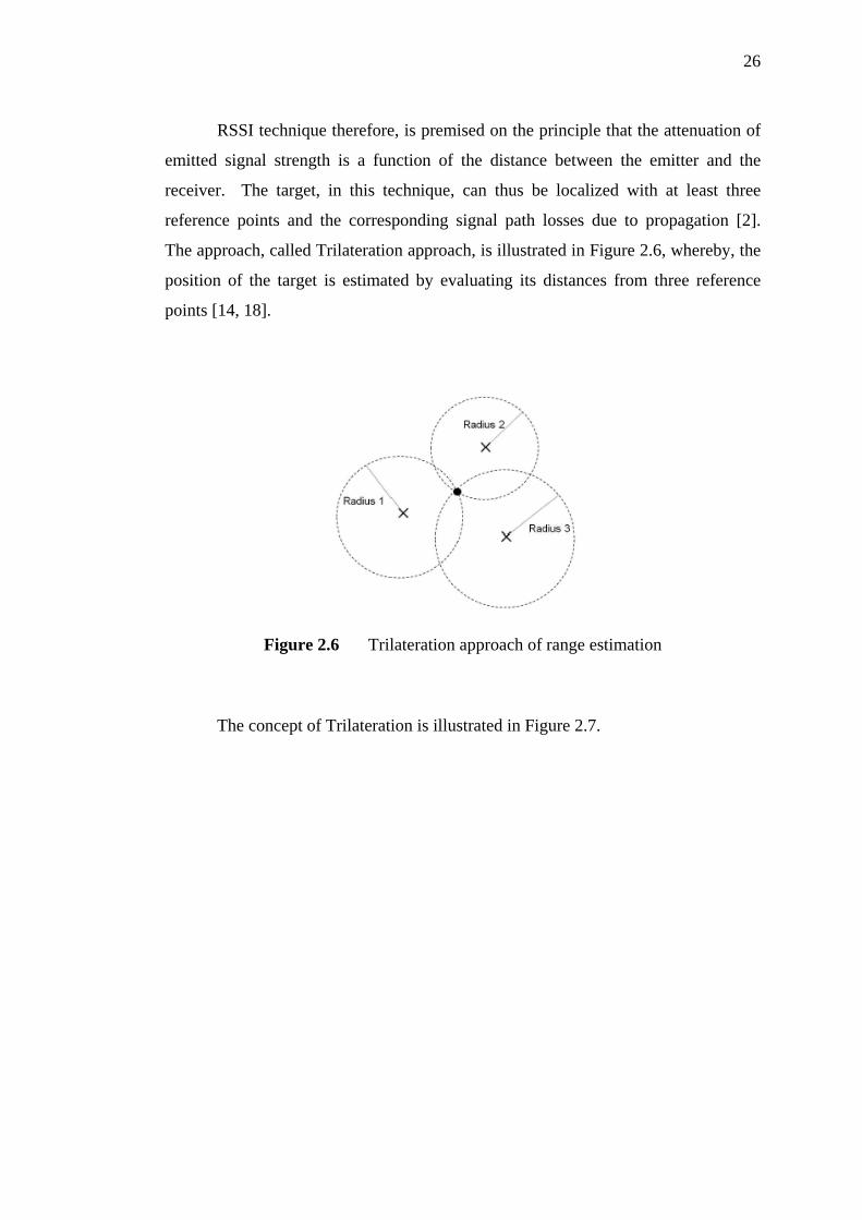
RSSI technique therefore, is premised on the principle that the attenuation of

emitted signal strength is a function of the distance between the emitter and the

receiver. The target, in this technique, can thus be localized with at least three

reference points and the corresponding signal path losses due to propagation [2].

The approach, called Trilateration approach, is illustrated in Figure 2.6, whereby, the

position of the target is estimated by evaluating its distances from three reference

points [14, 18].

Figure 2.6 Trilateration approach of range estimation

The concept of Trilateration is illustrated in Figure 2.7.

27

Figure 2.7 Basic node formulation in Trilateration

Referring to Figure 2.7, assuming that A1, A2 and A3 are the anchor nodes in

known locations while B is a blind node in an unknown location. Let coordinates of

A1, A2 and A3 be (x1,y1), (x2,y2) and (x3,y3) respectively while coordinate of B is (x,y).

Now, let us assume that distances between A1, A2 and A3 toward B are d1, d2 and d3

respectively. So, through Trilateration, coordinate x and y can be calculated as [3]:

)(

)(

23

231

xxyyyvx a

−−−

= (2.15)

and

))(())((

)()(

21232321

2123

xxyyxxyyxxvxxvy ab

−−−−−−−−

= (2.16)

where,

2

)()()( 23

22

23

22

23

22 yyxxddva

−−−−−= (2.17)

and

2

)()()( 21

22

21

22

21

22 yyxxddvb

−−−−−= [19] (2.18)

28

Several models have been proposed empirically and theoretically, in order to

translate the difference between the transmitted and the received signal strength into

distance estimation. The signal propagation theory behind RSSI can further be

understudied through the following topic, having further sub-topics:

2.3.5 Radio Interferometric Positioning System

The Radio Interferometric Positioning System (RIPS) is similar to the

proposed technique in that it employs dual-frequency for its operation [20].

The principle of optical interference is presently used in interferometers for

metrology, for high precision distance measurements over short distances and for the

definition of the meter. The development of interferometers dates back to 1880,

when A. A. Michelson had his first interferometer built in Germany [21]. A first

measurement of the meter in terms of light waves followed in 1889. For his work on

interferometers, Michelson received the Nobel Prize in Physics in 1907.

The basic principle of an interferometer is that two sinusoidal signals are

transmitted with slightly different frequencies. A reflecting tag (object) at the

unknown node reflects the signals back to the transmitter. The difference in the

frequencies of the arrived signals at the transmitter is then used to estimate the

location of the object.

29

The major drawback with this technique is that four (4) nodes are needed for

its successful operation. If one node fails, then the range becomes difficult to

estimate.

2.3.6 Swept Frequency technique

Other techniques such as Swept Frequency technique and Pulse Compression

technique have also been employed [7], to increase the unambiguous range though,

but the operational logistics and system requirements related to cost, hardware, and

real-time processing, make the realization of such techniques more tasking for urban

sensing applications [7].

Generally, the proposed dual-frequency technique however, will meet the

necessary requirements and is likely to emerge as one of the leading technologies in

a multipath environment [7].

2.4 The Proposed Technique

The proposed technique for this project work is similar to the principle of

operation of Radar (an acronym for Radio Detection And Ranging). The similarity

of both Radar and the proposed technique for this project work is that they both

employ dual-frequency to estimate ranges of objects. However, Radar operates using

30

2-way propagation scenario while the proposed technique for this project will operate

on one-way propagation scenario.

2.4.1 The principle of operation of Radar

Radar is an object detection system that uses radio waves to determine the

range, angle or velocity of objects. A Radar transmits radio waves that reflects from

any object in its path. The received waves are then processed to determine the above

named properties of the object.

The power returning to the receiving antenna is given by:

222

4

)4( rt

rttr RR

FAGPPπ

σ= (2.19)

where Pt = transmitted power,

Gt = gain of transmitting antenna,

σ = Radar cross-section,

F = pattern propagation factor,

31

Rt = distance from the transmitter to target,

Rr = distance from the target to the receiver,

Ar = effective aperture (area) of receiving antenna given by:

πλ

4

2r

rGA = (2.20)

where λ = transmitted wavelength, and

Gr = gain of receiving antenna.

However, in common case where transmitter and receiver are at the same

location, then

Rt = Rr (2.21)

which implies that:

42

4

)4( RFAGPP rtt

r πσ

= (2.22)

32

2.4.2 Range estimation based on Dual-frequency signaling

Consider that a dual-frequency signal is transmitted from a transmitter using

frequencies f1 and f2 to an object [22], located at an unknown point, as shown in

Figure 2.8. The transmitted signals at frequency fi, i = 1, 2, can be expressed as [16],

)()( 0)( tntji

iets +−= φρ , i = 1, 2, (2.23)

where si(t) is the dual-frequency waveforms from the transmitter,

ρ is the range-dependent amplitude,

)(tiφ is phase of the signal corresponding to the i-th frequency of operation,

and

n0(t) is the Gaussian noise introduced into the signals [22].

33

Figure 2.8 Transmission of dual-frequency from a reader to an object

Now,

)(2)( xtft ii += πφ (2.24)

Measuring both phases in the [0, π2 ] range, then we have

mtft ππφ 22)( 11 += (2.25)

and

ntft ππφ 22)( 22 += (2.26)

Now, the velocity of electromagnetic wave propagation is related to both the

time of arrival of the signal from the transmitter to the receiver [23], and also the

distance between the transmitter and the receiver as follows:

ttRc )(

= , (2.27)

where c = the velocity of electromagnetic wave propagation,

34

R(t) = the desired range, and

t = time of arrival of the signal from the transmitter to the receiver.

From equation (2.27),

ctRt )(

= (2.28)

Substituting Equation (2.28) into Equations (2.25) and (2.26) gives,

mc

tRft ππφ 2)(2)( 11 += , (2.29)

and

nc

tRft ππφ 2)(2)( 22 += (2.30)

where m and n are unknown integers.

Now, the phase difference at the receiver, from Equations (2.29) and (2.30) is

given by:

)()()( 12 ttt φφφ −=∆ (2.31)

= nc

tRf ππ 2)(2 2 + − mc

tRf ππ 2)(2 1 −

= ( ) ( )nmffc

tR−−− ππ 2)(2

12 (2.32)

35

Making R(t) the subject of the expression in Equation (2.17) gives,

)()(

)(2)()(

1212 ffnmc

fftctR

−−

−−

∆=

πφ (2.33)

The second term in Equation (2.33) induces ambiguity in range, which means

that for the same phase difference, the range estimate can assume infinite values [16]

separated by the maximum unambiguous range Rmax [22]. An example of the phase

difference versus the range estimate is shown in Figure 2.7, where the frequency

separation is f∆ = 26 MHz and the actual range is R = 7.6 m [22]. So, to remove this

ambiguity, we assume that nm = . Hence, Equation (2.33) reduces to,

ftctR

∆∆

=πφ

2)()( [7] (2.34)

where 12 fff −=∆ [13, 21].

However, the maximum unambiguous range is given by [24]:

f

cR∆

=2max (2.35)

6

8

10262103xx

x=

= 5.77 m

36

Figure 2.9 Phase difference versus Range estimate

For clarity, the actual range (R) at 7.6 m is marked by a square and the

estimated ranges at repetitive positions 1.83 m, 13.37 m, 19.14 m, . . ., separated by

Rmax = 5.77 m are marked by circles [22].

37

CHAPTER 3

METHODOLOGY

3.1 Introduction

The methodology involves a body of methods, rules, and postulates employed

in carrying out this work. It captures the analysis of the principles or procedures of

inquiry into the field of ranging estimation.

This project work is carried out following the schedule outlined below:

(1) Critical understudying the signal propagation processes and techniques.

(2) a) Reviewing the previous work done, including the techniques which have

been developed.

b) Understudying through research, the approach of the employed dual-

frequency technique.

(3) Carrying out simulations of PDoA in the Matlab environment.

(4) Studying and analyzing the phase characteristics of the received signal.

38

(5) Analyzing the Range ambiguity, effect of noise and error on the range

estimation.

(6) Drawing out the findings.

Figure 3.1 captures the above schedule in flowchart form.

Figure 3.1 Flowchart describing the project schedule

39

3.2 Tools of Research

The employable tools available for carrying out this research work are

basically:

(1) Matlab, for simulation, and

(2) Universal Software Radio Peripheral.

3.2.1 Matlab

MATLAB (which stands for MATrix LABoratory) is a high-level technical

computing language and interactive environment for algorithm development, data

visualization, data analysis, and numerical computation. It is a special-purpose

computer program optimized to perform Engineering and scientific calculations.

Using Matlab, technical computing problems can be solved faster, especially when

interfaced with programs written in programming languages such as C, C++, Java,

Python and Fortran.

Matlab is more than a fancy calculator. It is an extremely useful and versatile

tool in Communication Engineering simulation. Even if a little is known about

Matlab, one can use it to accomplish wonderful things. The hard part, however, is

figuring out which of the hundreds of commands, scores of help pages, and

thousands of items of documentation one needs to look at to start using it quickly and

efficiently.

40

Many signal processing researchers now use the Matlab technical computing

language to develop their algorithms because of its ease to use, powerful library

functions and convenient visualization tools.

The aim here is not to go into the details of the operations of Matlab, but to

mention it as a tool employed for simulation in this project work. The codes for the

simulations of this work are presented in the Appendices.

3.2.2 Universal Software Radio Peripheral

The Universal Software Radio Peripheral (USRP) is a transceiver device

which enables engineers to rapidly design and implement powerful and flexible

software radio systems [25]. Figure 3.2 shows the board diagram of a USRP. The

intuitive USRP design, coupled with a broad selection of daughter-boards covering a

wide range of frequencies, helps in getting the needed software radio up and running

quickly.

41

Figure 3.2 Universal Software Radio Peripheral

What is simply needed is to download GNU Radio, a complete open source

software radio and signal processing package, and the USRP is ready to use. Once

the software is installed and the USRP is plugged into a host computer, it is ready to

transmit and receive a virtually limitless variety of signals. The USRP can

simultaneously receive and transmit on two antennas in real time. All sampling

clocks and local oscillators are fully coherent, thus allowing the creation of MIMO

(Multiple-Input, Multiple-Output) systems [26].

42

In the USRP, high sample-rate processing takes place in the Field

Programmable Gate Array (FPGA), while lower sample-rate processing happens in

the host computer. The two onboard Digital Down-Converters (DDCs) mix, filter,

and decimate (from 64 MS/s) incoming signals in the FPGA. Two Digital Up-

Converters (DUCs) interpolate baseband signals to 128 MS/s before translating them

to the selected output frequency. The DDCs and DUCs combined with the high

sample rates also greatly simplify analog filtering requirements. Daughterboards

mounted on the USRP provide flexible, fully integrated RF front-ends. A wide

variety of available daughterboards allows the use of different frequencies for a

broad range of applications. The USRP accommodates up to two RF transceiver

daughterboards (or two transmit and two receive) for RFI/O.

The features of USRP include the following:-

(1) Four 64 MS/s 12-bit analog to digital converters,

(2) Four 128 MS/s 14-bit digital to analog converters,

(3) Four Digital Down-Converters with programmable decimation rates,

(4) Two Digital Up-Converters with programmable interpolation rates,

(5) High-speed USB 2.0 interface (480 Mb/s),

(6) Capable of processing signals up to 16 MHz wide,

(7) Modular architecture supports wide variety of RF daughterboards,

(8) Auxiliary analog and digital I/O support complex radio controls such as RSSI

and AGC,

(9) Fully coherent multi-channel systems (MIMO capable) [27].

The operational principle for the experimental set-up of USRP is described as

follows:

The set-up is usually carried out as sown in Figure 3.3. In the set-up, 2.4

GHz is usually chosen as the centre-frequency because of its suitability for Amateur

Radio, Microwave link and Radar. Furthermore, it is a common knowledge that the

43

2.4 GHz band has been set aside for industrial, Scientific and Medical (ISM)

purposes due to its use in microwave heating. Both transmitter and receiver are set at

a height of 1 meter from the ground level. Single-tone (sinusoidal) signal is then sent

from the transmitter to the receiver (which does not require modulation) and various

values of the received power are obtained for

(i) free space model,

(ii) log-normal shadowing model, and

(iii) two-ray ground model

for distances of 1 m, 3 m, 5 m, 7 m, 9 m, 11 m, 13 m, 15 m, 17 m and 19 m. The

result is discussed in Chapter 4.

Figure 3.3 Experimental set-up of USRP

44

3.3 Possible obstacles to localization accuracy

Obstacles to localization accuracy of an object include environmental

interferences and occlusions (e.g., the presence of liquids and metals), orientation

and spatial arrangement of an object, ambient RF noise and readers' locations. These

factors can weaken, scatter, or occlude radio waves, and thus lead to unreliable

detection and inaccurate positioning of objects [12].

Previous techniques tend to sacrifice speed and accuracy in localizing objects

in order to obtain reliable estimates. That is by carrying out repeated measurements

that should consistently yield the same outcome. Unfortunately, these resulting

speed and accuracy degradations tend to reduce the efficacy of the performance.

However, the proposed localization framework will enable accurate object position

estimation, without compromising either speed or reliability. This is because the

proposed framework is highly scalable and can accommodate a wide range of

requirements and tradeoffs among power, cost, accuracy and speed.

45

CHAPTER 4

SIMULATION RESULTS AND ANALYSIS

4.1 Simulation Set-up

The Simulation of this work was carried out in Matlab environment [28].

The simulation results are hereby presented in this Chapter. Furthermore, each

presented result is analyzed for the sake clarity.

First, Equation (2.34) was simulated in order to observe the graphical relation

between phase-difference and distance. Figure 4.1 was obtained in the process,

which shows that the range is directly proportional to the phase difference between

two signals emanating from the transmitter.

46

Figure 4.1 Phase Difference Vs. Distance Relation

Next, the simulation was set-up, to obtain the Dual-frequency estimator

results. Here, two pairs of operating frequencies were used with the following

parameters:

Center frequency, cf = 2.4 GHz,

Lower frequency, 1f = 2ffc

∆− (4.1)

and,

Upper frequency, 2f = 2ffc

∆+ (4.2)

Table 4.1 presents the results of the lower and upper frequencies, obtained for

the various values of frequency difference, f∆ .

Table 4.1 The operating frequencies used for Simulation

f∆ (MHz) f1(GHz) f2(GHz) 0.5 2.39975 2.40025 5 2.3975 2.4025 50 2.375 2.425 500 2.15 2.65

47

These frequencies different selections were evaluated in terms of phase

difference for range cover, up till 600 meters [3]. The dual-frequency estimator

results in Figure 4.2 were obtained.

Figure 4.2 Dual-frequency Estimator results

It could be seen from Figure 4.2 that with centre-frequency fc at 2.4 GHz, five

different levels of frequency difference run on the Matlab produced varying

sinusoids, each having different impact on the required range.

Further, the simulation set-up was carried out for the various propagation

madels as follows:

48

4.2 Propagation models simulation results

Equations (2.11), (2.12) and (2.14) were simulated in Matlab environment for

the Two-ray model, Log-normal Shadowing model and Free-space model

respectively. Furthermore, experimental set-up was carried out to see signal

propagation using USRP as well. Received power were read at distances 1 m, 3 m, 5

m, 7 m, 9 m, 11 m, 13 m, 15 m, 17 m and 19 m. The simulation results are as shown

in Figure 4.3.

It could be seen from the results of Figure 4.3 that the free-space propagation

model is close to the USRP result. This shows the acceptability and reliability of

free-space model in the one-way short-range propagation scenario.

Figure 4.3 Propagation models graphs

49

The result analysis is further carried out via range ambiguity, the effect of

noise and error analysis in the following subsections.

4.3 Range ambiguity

The equation which generates the phase difference of two signals with

different frequencies is obtained as follows:

ii nff wt φϕθ +∆+=∆ 0 (4.3)

where,

)(2 12 ffw −=∆ π (4.4)

)2()2( 11102220 nffnff tftf φπϕφπϕθ ++−++=∆∴ (4.5)

where if0ϕ is the phase for each frequency carrier, and

infφ is the phase noise generated using normally distributed noise with

variance of 150 which use to exist in a practical scenario [3].

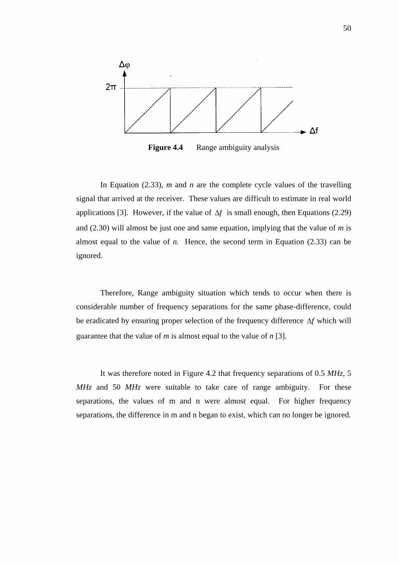
Now, on the issue of the range ambiguity which was being introduced into

the system by the second term in Equation (2.33). Figure 4.4 shows that for a

particular phase difference )(tφ∆ , there could be infinite values of range estimate

R(t), separated from each other by f

nmc∆− )( .

50

Figure 4.4 Range ambiguity analysis

In Equation (2.33), m and n are the complete cycle values of the travelling

signal that arrived at the receiver. These values are difficult to estimate in real world

applications [3]. However, if the value of f∆ is small enough, then Equations (2.29)

and (2.30) will almost be just one and same equation, implying that the value of m is

almost equal to the value of n. Hence, the second term in Equation (2.33) can be

ignored.

Therefore, Range ambiguity situation which tends to occur when there is

considerable number of frequency separations for the same phase-difference, could

be eradicated by ensuring proper selection of the frequency difference f∆ which will

guarantee that the value of m is almost equal to the value of n [3].

It was therefore noted in Figure 4.2 that frequency separations of 0.5 MHz, 5

MHz and 50 MHz were suitable to take care of range ambiguity. For these

separations, the values of m and n were almost equal. For higher frequency

separations, the difference in m and n began to exist, which can no longer be ignored.

51

However, phase ambiguity exists since the value of phase can only be

measured in the range of [ ππ ,− ] [3]. This is shown in Figure 4.5, as phase

difference changes over time and time is related to distance.

Figure 4.5 Phase difference of two signals with time

4.4 Effect of Phase Noise

Noise is a term generally used to refer to any spurious or undesired

disturbances that mask the received signal in a communication system. Noise, in a

communication system, is otherwise referred to Interference.

Phase noise is the result of small random fluctuations or uncertainty in the

phase of an electronic signal. Such interference was therefore introduced into the

52

phase of the transmitted signal and sent together with the wanted signal, in order

understudy its effect on the propagation scenario via ranging estimation.

Figure 4.6 presents the simulated graphs obtained for various frequency-

differences of 10MHz, 1MHz and 0.5MHz, for both ‘Noisy’ signals and ‘No-noise’

signals.

Figure 4.6 Effect of phase noise on the signal propagation

From Figure 4.6, it could be seen that at No-noise,

for 10 MHz,

metersd )59( −=∆

meters4=

and

53

0)12()( −=∆ tφ

01=

Therefore, if 10 corresponds to 4 meters,

then, 150 would correspond to (4 x 15) meters = 60 meters.

Secondly,

for 1 MHz,


meters10=

and

02.0)( =∆ tφ

Therefore, if 0.20 corresponds to 10 meters,

then, 150 would correspond to 152.0

10 x meters = 750 meters.

Also,

for 0.5 MHz,


meters18=

and

02.0)( =∆ tφ

Therefore, if 0.20 corresponds to 18 meters,

then, 150 would correspond to 152.0

18 x meters = 1350 meters.

54

Furthermore, Figure 4.7 shows the plot of values of phase difference with

corresponding values of distance from 1 meter to 500 meters.

Figure 4.7 Phase difference over 500 meters

It could be seen from Figure 4.7 that )(tφ∆ is not identical to each other for

smaller values of f∆ . Specifically, for f∆ = 0.5 MHz and f∆ = 5 MHz, suitability is

guaranteed for the propagation within 500 meters. Frequency difference of f∆ = 50

MHz, is suitable within 100 meters. For higher frequency difference, )(tφ∆ is easily

affected by noise. This is because the proportionality between the phase difference

and distance is not direct unlike in the case of the lower frequency difference. This

further confirms that lower values of f∆ are suitable for short-range application

since the value of )(tφ∆ will not vary much from the real expected value [3].

55

4.5 Error Analysis

The errors were analyzed via distance error and phase error. Table 4.2

presents the obtained results, the simulation of which produced Figure 4.8.

Table 4.2 Distance error Vs Phase error

Phase error (0) Distance error(m) 0.001 2.5 0.005 2.5 0.01 2.5 0.05 2.5 0.1 2.8 0.5 5 1 10 5 25 10 50 50 240

Figure 4.8 Distance error Vs Phase error graph

56

It could be deduced from the graph of Figure 4.8 that the employed dual-

frequency technique for range estimation is very suitable for short range application

of within 100 meters (corresponding to 150 phase error) at lower frequency

separations of up to 50 MHz.

57

CHAPTER 5

CONCLUSION

5.1 Introduction

This chapter concludes the project development through a re-cap of the

objectives set out for this work, the simulated results and analysis, and

recommendations are offered for future improvement of Ranging estimation.

5.2 Conclusion

In this work, the employed dual-frequency technique provides the capability

of estimating the range of objects over a short-range application. This is because

Range estimation is important to providing localization and tracking of assets and

objects in various applications. The objectives set for this work were achieved

through:

58

(i) adequate understudying the signal propagation via free-space

propagation model, log-normal propagation model and two-ray

propagation model,

(ii) carrying out simulations in Matlab environment; results being

presented in Chapter 4,

(iii) analyzing the range ambiguity and effect of noise on the range

estimation, also in Chapter 4.

The basic concept introduced in this dual-frequency ranging technique is that

when two different signals travel from a transmitter Tx and arrive at the receiver Rx,

the phase difference between these two signals at the receiver can be used to estimate

the distance between the transmitter and the receiver.

As discussed in sections 4.3 and 4.4, the phase difference, )(tφ∆ has direct

relation with the frequency difference, f∆ , which must not be too high in order to

avoid range ambiguity, and to drastically reduce the influence of noise on the result.

From the simulations results therefore, lower frequency difference of up to 50

MHz is very suitable for short-range ranging estimation application of within 100

meters.

5.3 Recommendation for Future work

Having achieved the objectives set out for this work, there is however, room

for further improvement. This is because of the enormous importance which the

59

subject of range estimation offers in the propagation environment in particular and

communication industry in general. The following recommendations are therefore

humbly made.

(i) It is recommended that the work be carried out as well for a long-range

application in a multipath environment.

(ii) Field measurement is recommended to be done using USRP, and the

results be compared with the Matlab simulated results.

(iii) The effect of synchronization is also recommended for investigation in a

non line-of-sight propagation environment.

60

REFERENCES

1. Suzhe, W. and Yong, L. Node localization algorithm based on RSSI in

wireless sensor network. Signal Processing and Communication System

(ICSPCS), 2012. 6th International Conference. IEEE, 2012.

2. Shi, Q., Correal, N., Kyperountas, S., and Niu, F. (2005). Performance

comparision between TOA ranging technologies and RSSI ranging

technologies for multi-hop wireless networks. In Vehicular Technology

Conference, 2005. VTC-2005-Fall. 2005 IEEE 62nd (Vol. 1, pp. 434-438).

IEEE.

3. Hassan, N. A. C., Yusof, K. M., and Yusof, S. K. S. (2015, August). Ranging

Estimation Using Dual-Frequency Doppler Technique. In IT Convergence

and Security (ICITCS), 2015 5th International Conference on (pp. 1-5).

IEEE.

4. Barsocchi, P., Lenzi, S., Chessa, S., and Giunta, G. (2009, April). A novel

approach to indoor RSSI localization by automatic calibration of the wireless

propagation model. In Vehicular Technology Conference, 2009. VTC Spring

2009. IEEE 69th (pp. 1-5). IEEE.

61

5. Scherhaufl, M., Pichler, M., Muller, D., Ziroff, A. and Stelzer, A. Phase-of-

arrival-based localization of passive UHF RFID tags. Microwave Symposium

Digest (IMS), 2013 IEEE MTT-S International. IEEE, 2013.

6. Andreas, P, Miesen, R, and Vossiek, M. Inverse sar-approach for localization

of moving rfid tags. RFID (RFID), 2013 IEEE International Conference on.

IEEE, 2013.

7. Ahmad, F., Amin, M. G., and Zemany, P. D. (2009). Dual-frequency radars

for target localization in urban sensing. IEEE transactions on aerospace and

electronic systems, 45(4), 1598-1609.

8. Armoogum, V., Soyjaudah, K. M. S., Mohamudally, N., and Fogarty, T.

(2007, May). Comparative study of path loss using existing models for digital

television broadcasting for summer season in the north of mauritius. In

Telecommunications, 2007. AICT 2007. The Third Advanced International

Conference on (pp. 34-34). IEEE.

9. Rachelin, S. P. and Saravanan, T. Target Tracking in Wireless Sensor

Networks Using ICTP and Miss Mechanism. Middle-East Journal of

Scientific Research vol. 20, no.12. 2014.

10. Mustafa, M. Y., Eilertsen, S. M., Hansen, I., Pettersen, E., and Kronen, A.

(2013, March). Matching mother and calf reindeer using wireless sensor

networks. In Computer Science and Information Technology (CSIT), 2013 5th

International Conference on (pp. 99-105). IEEE.

11. Hekmat, R. (2006). Modeling Ad-hoc Networks. Ad-hoc Networks:

Fundamental Properties and Network Topologies, 15-39.

62

12. Lu, Y., Zhang, W., Meng, Y., and Yu, H. (2011, December). A novel

approach for accurately and quickly localizing a tag from a mass of passive

RFID tags. In Intelligent Sensors, Sensor Networks and Information

Processing (ISSNIP), 2011 Seventh International Conference on (pp. 485-

489). IEEE.

13. Bouet, M. and Aldri, L. D. S. RFID tags: Positioning principles and

localization techniques. Wireless Days, 2008. WD'08. 1st IFIP. IEEE, 2008.

14. Mao, G., Fidan, B. and Anderson, B. D. Wireless sensor network localization

techniques. Computer networks, vol. 51, no. 10. 2007.

15. Oguejiofor, O., Aniedu, A., Ejiofor, H. and Okolibe, A. Trilateration based

localization algorithm for wireless sensor network. International Journal of

Science Mod. Engineering, vol. 97, no. 2. 2009.

16. Zhang, Y., Amin, M., and Ahmad, F. (2007, November). A novel approach

for multiple moving target localization using dual-frequency radars and time-

frequency distributions. In Signals, Systems and Computers, 2007. ACSSC

2007. Conference Record of the Forty-First Asilomar Conference on (pp.

1817-1821). IEEE.

17. Tan, D. K. P., Lesturgie, M., Sun, H. and Lu, Y. Moving target localization

using dual-frequency continuous wave radar for urban sensing applications.

Radar Conference-Surveillance for a Safer World, 2009. RADAR.

International. IEEE, 2009.

18. Wang, L., Argumedo, A., and Washington, W. (2014). Precise asymptotic

distribution of the number of isolated nodes in wireless networks with

lognormal shadowing. Applied Mathematics, 5(15), 2249.

63

19. Cheng, L., Wu, C., Zhang, Y., Wu, H., Li, M., and Maple, C. (2012). A

survey of localization in wireless sensor network. International Journal of

Distributed Sensor Networks, 2012.

20. Shang, J., Yu, S., and Zhu, L. (2009, January). Location-aware systems for

short-range wireless networks. In Computer Network and Multimedia

Technology, 2009. CNMT 2009. International Symposium on (pp. 1-5). IEEE.

21. Maroti, M., Volgyesi, P., Dora, S., Kusy, B., Nadas, A., Ledeczi, A., Balogh,

G. and Molnar, K. Radio interferometric geolocation. Proceedings of the 3rd

international conference on Embedded networked sensor systems. ACM,

2005.

22. Bölcskei, H. (2001). Blind estimation of symbol timing and carrier frequency

offset in wireless OFDM systems. Communications, IEEE Transactions on,

49(6), 988-999.

23. Zhang, Y., Amin, M., and Ahmad, F. (2008). Time-frequency analysis for the

localization of multiple moving targets using dual-frequency radars. Signal

Processing Letters, IEEE, 15, 777-780.

24. Yusof, K. M. and Fitz, S. Short range frequency estimation for localization in

cognitive radio environment. International Conference on Computer

Communication Networks, ICCCN 2011. IEEE, 2011.

25. Ahmad, F., Amin, M. G. and Zemany, P. D. Performance analysis of dual-

frequency CW radars for motion detection and ranging in urban sensing

64

applications. Defense and Security Symposium. International Society for

Optics and Photonics, 2007.

26. Akiyama, T., Nakamura, M., Sugimoto, M. and Hashizume, H. Smart phone

localization method using dual-carrier acoustic waves. Indoor Positioning

and Indoor Navigation (IPIN), 2013 International Conference. IEEE, 2013.

27. Kambiz, S., Soltan, M. and Moshfeghi, M. Method and system for

determining the distance between an RFID reader and an RFID tag using

phase. U.S. Patent Application 11/641,623. 2006.

28. Leong, K. S., Ng, M. L., and Cole, P. H. (2006, January). Positioning analysis

of multiple antennas in a dense RFID reader environment. In Applications

and the Internet Workshops, 2006. SAINT Workshops 2006. International

Symposium on (pp. 4-pp). IEEE.

APPENDICES

65

APPENDIX A

RANGE VERSUS PHASE-DIFFERENCE CODE

x=0:20:200;

y=2*pi*10*10^6*x/(3*10^8);

plot(x,y);

title('Plot of y=2*pi*f*x/c');

xlabel('Range(m)');

ylabel('Phase difference(rad)');

grid on;

66

APPENDIX B

CODE FOR THE EFFECT OF NOISE ON SIGNAL PROPAGATION

f1 = 2.4e9 - 5e6;

f2 = 2.4e9 + 5e6;

f3 = 2.4e9 - 0.5e6;

f4 = 2.4e9 + 0.5e6;

f5 = 2.4e9 - 0.25e6;

f6 = 2.4e9 + 0.25e6;

D = 1:2:20;

C = 3*10^8;

time = D / C ;

%niadalah phase of the signal tanpa noise.

P12 = ((2*pi*f2)-(2*pi*f1))*time; % phase difference of 2 freq10Mhz

P34 = ((2*pi*f4)-(2*pi*f3))*time; %1MHz

P56 = ((2*pi*f6)-(2*pi*f5))*time; %0.5MHz

sz = size(time);

theta1n1 = (2*pi*f1*time) + (sqrt((15/180)*pi))*randn(sz) + mean(P12);


P12_noise = theta2n1 - theta1n1;

67



P12_noise1 = theta2n2 - theta1n2;



P12_noise2 = theta3n1 - theta1n3;

d12 = 2*pi*(f2-f1);

d21 = C / d12;

df_noise = (d21* P12_noise);

de_noise = D - df_noise;

d34 = 2*pi*(f4-f3);

d43 = C / d34;

df_noise1 = (d43* P12_noise1);

de_noise1 = D - df_noise1;

d56 = 2*pi*(f4-f3);

d65 = C / d56;

df_noise2 = (d65* P12_noise2);

de_noise2 = D - df_noise2;

figure

set(gcf,'color','white')

plot (D,P12,'-*',D,P12_noise,'-o',D,P12_noise1,'-rs',D,P34,'k-^',D,P56,'y-

+',D,P12_noise2,'g->')

legend('No Noise 10MHz','Noise 10MHz','No Noise 1MHz','Noise

1MHz','No Noise 0.5MHz','Noise 0.5MHz','location','northwest')

xlabel('Distance (meter)')

ylabel('phase difference (degree)')

%ylim([-2 2])

figure


plot (D,de_noise,'-o',D,de_noise1,'-rs',D,de_noise2,'-^')

68

legend('Noise 10MHz','Noise 1MHz','Noise 0.5MHz','location','southeast')

xlabel('Distance (meter)')

ylabel('error (meter)')

grid on

69

APPENDIX C

DISTANCE ERROR VERSUS PHASE ERROR CODE

a = [3 5 6 9 12 15 18 21 24 27 30]; % no of sample

b = [0.504451366 0.362985993 0.238900961 0.161617728 0.139045787

0.133009991 0.125743177 0.110583847 0.098528411 0.112143764

0.115902647]; %rmsemle

c = [0.337411172 0.277563097 0.404998642 0.433410245 0.450832963

0.461374771 0.467663081 0.472027563 0.476732891 0.479692366

0.482266363]; %rmselse

d = [0.742884929 0.839563265 2.542814286 0 5.206404177 12.1570605

14.58707658 16.20275377 23.5151271 25.29466008 25.17918633];

%rmsecrt

figure


set (0, 'DefaultAxesFontSize', 8, 'DefaultAxesFontName','Arial');

% set (0,'DefaultAxesLineStyleOrder',{'-',':','--'})

% figure;

set (gcf, 'Units', 'centimeter');

pos = get (gcf, 'Position');

pos(3) = 10; % figure box size 9.7cm x 6.3cm

70

pos(4) = 7.5; % default 6.3

set (gcf, 'Position', pos);

set (gca, 'Units', 'centimeter');

set (gca, 'Position', [1.3 0.9 8 5]); %axes box size 8cm x 5cm

subplot(3,1,1)

plot (a,b,'-*b')

legend ('MLE')

ylabel('RMSE')

xlim ([2 31])

ylim ([0 0.6])

subplot(3,1,2)

plot (a,c,'-or')

legend ('LSE')

ylabel('RMSE')

xlim ([2 31])

ylim ([0.1 0.6])

subplot(3,1,3)

plot (a,d,'-+g')

ylim ([-3 27])

xlim ([2 31])

legend ('CRT')

xlabel('sample')

ylabel('RMSE')

a = [0.20943951 0.628318531 1.047197551 1.466076572 1.884955592

2.303834613 2.722713633 3.141592654 3.560471674 3.979350695]; % real

phase

b = [0.2736 0.7914 0.9894 2.1336 2.5006 1.9921 2.6728 3.0596 3.7129

4.5532]; % estimate phase mle

c = [0.187833319 0.652675043 1.1317 2.012061032 2.361914555 2.1975769

2.857003533 3.25493212 3.377071674 4.380370948]; % estimate phase lse

71

d = [0.1951 0.6125 0.1504 0.9405 1.793 1.9552 0.9256 2.6312 3.2301

2.4832]; % estimate phase crt

figure




% figure;




pos(4) = 7.5; % default 6.3




plot (a,a,'-k',a,b,'-*b',a,c,'-or',a,d,'-+g')

ylim ([0 4.7])

xlim ([0.1 4.1])

legend ('Actual Phase','MLE','LSE','CRT')

xlabel('Real Phase in degree')

ylabel('Estimate Phase in degree')

title('Estimate Phase vs Real Phase')

a = [1 3 5 7 9 11 13 15 17 19]; %real distance

b = [1.306343773 3.778656659 4.724037021 10.1871896 11.93948552

9.511576864 12.76167996 14.60851392 17.72779165 21.73992861]; %

estimate distance mle

c = [0.896838036 3.11629378 5.403469473 9.606883771 11.2773113

10.49265679 13.64118704 15.54115609 16.1243295 20.91473067]; %

estimate distance lse

d = [0.931533882 2.924472079 0.718107103 4.49E+00 8.560944389

72

9.335392342 4.41941446 12.56305459 15.42259145 11.85640664]; %

estimate distance crt

figure




% figure;




pos(4) = 7.5; % default 6.3




plot (a,a,'-k',a,b,'-*b',a,c,'-or',a,d,'-+g')

ylim ([0.5 22])

xlim ([0.5 19.5])

legend ('Actual Distance','MLE','LSE','CRT')

xlabel('Actual Distance in meter')

ylabel('Estimate Distance in meter')

title('Estimate Distance vs Real Distance')

a = [0.001 0.005 0.01 0.05 0.1 0.5 1 5 10 50]; % phase error

b = [0.004774648 0.023873241 0.047746483 0.238732415 0.477464829

2.387324146 4.774648293 23.87324146 47.74648293 238.7324146]; %

Distance error

figure


semilogx(a,b,'b-*','LineWidth',2)

ylim ([-1 250])

73

xlabel('Phase error in degree')

ylabel('Distance error in meter')

a = [1 2 3 4 5 6 7 8 9 10 11 12 13 14 15 16 17 18 19 20 21 22 23 24 25 26 27

28 29 30 31 32 33 34 35 36 37 38 39 40 41 42 43 44 45]; % phase error

b=[4.77464829275686,9.54929658551372,14.3239448782706,19.098593171

0274,23.8732414637843,28.6478897565412,33.4225380492980,38.1971863

420549,42.9718346348117,47.7464829275686,52.5211312203255,57.29577

95130823,62.0704278058392,66.8450760985960,71.6197243913529,76.394

3726841098,81.1690209768666,85.9436692696235,90.7183175623803,95.4

929658551372,100.267614147894,105.042262440651,109.816910733408,11

4.591559026165,119.366207318921,124.140855611678,128.915503904435,

133.690152197192,138.464800489949,143.239448782706,148.01409707546

3,152.788745368220,157.563393660976,162.338041953733,167.112690246

490,171.887338539247,176.661986832004,181.436635124761,186.2112834

17518,190.985931710274,195.760580003031,200.535228295788,205.30987

6588545,210.084524881302,214.859173174059]; % Distance error

figure




% figure;




pos(4) = 7.5; % default 6.3




plot(a,b,'m-^')

%ylim ([-1 250])

74

xlabel('Phase error in degree')

ylabel('Distance error in meter')

legend ('Distance = 15m')

xlim ([0 47])

title('Distance Error vs Phase Error')

range estimation using phase difference of...

Documents