randomized algorithms - tutelomaa/teach/randal-15-1.pdf · a randomized min-cut algorithm 2....

1/15/2015

1

Randomized Algorithms

Prof. Tapio Elomaa

[email protected]

Course Basics

• A new 4 credit unit course• Part of Theoretical Computer Science

courses at the Department of Mathematics• There will be 4 hours of lectures per week• Weekly exercises start next week• We will assume familiarity with

– Necessary mathematics– Basic programming

15-Jan-15MAT-72306 RandAl, Spring 2015 2

1/15/2015

2

Organization & Timetable

• Lectures: Prof. Tapio Elomaa– Tue & Thu 12–14 in TB219 & TB223– Jan. 13 – Mar. 5, 2015– Exception: Thu Feb. 5 TD308 12–13

• Exercises: M.Sc. Juho LauriMon 10–12 TC315

• Exam: Wed. Mar. 11, 2015


Course Grading


• Exam: Maximum of 30 points• Weekly exercises yield extra points

• 40% of questions answered: 1 point• 80% answered: 6 points• In between: linear scale (so that

decimals are possible)

1/15/2015

3

Material

• The textbook of the course is– Michael Mitzenmacher & Eli Upfal: Probability

and Computing, 3rd ed., MIT Press, 2009• There is no prepared material, the slides

appear in the web as the lectures proceed– http://www.cs.tut.fi/~elomaa/teach/72306.html

• The exam is based on the lectures (i.e., noton the slides only)


Content (Plan)

1. Events and Probability2. Discrete Random Variables and Expectation3. Moments and Deviations4. Chernoff Bounds5. Balls, Bins, and Random Graphs6. The Probabilistic Method7. Markov Chains and Random Walks8. Continuous Distributions and the Poisson Process9. Entropy, Randomness, and Information10. The Monte Carlo Method


1/15/2015

4

1. Events and Probability

Verifying Polynomial IdentitiesAxioms of Probability

Verifying Matrix MultiplicationA Randomized Min-Cut Algorithm

2. Discrete RandomVariables and Expectation

Random Variables and ExpectationThe Bernoulli and Binomial Random

VariablesConditional Expectation

The Geometric DistributionThe Expected Run-Time of Quicksort

1/15/2015

5

3. Moments and Deviations

Markov's InequalityVariance and Moments of a Random

VariableChebyshev's Inequality

A Randomized Algorithm forComputing the Median

4. Chernoff Bounds

Moment Generating FunctionsDeriving and Applying Chernoff BoundsBetter Bounds for Some Special Cases

Set Balancing

1/15/2015

6

5. Balls, Bins, andRandom Graphs

The Birthday ParadoxBalls into Bins

The Poisson DistributionThe Poisson Approximation

HashingRandom Graphs

6. The ProbabilisticMethod

The Basic Counting ArgumentThe Expectation Argument

Derandomization Using ConditionalExpectations

Sample and ModifyThe Second Moment Method

The Conditional Expectation InequalityThe Lovasz Local Lemma

1/15/2015

7

7. Markov Chains andRandom Walks

Markov Chains: Definitions andRepresentations

Classification of StatesStationary Distributions

Random Walks on Undirected GraphsParrondo's Paradox

8. Continuous Distributionsand the Poisson Process

Continuous Random VariablesThe Uniform Distribution

The Exponential DistributionThe Poisson Process

Continuous Time Markov ProcessesMarkovian Queues

1/15/2015

8

9. Entropy, Randomness,and Information

The Entropy FunctionEntropy and Binomial Coefficients

Entropy: A Measure of RandomnessCompression

10. The Monte CarloMethod

The Monte Carlo MethodThe DNF Counting Problem

From Approximate Sampling toApproximate Counting

The Markov Chain Monte Carlo Method

1/15/2015

9

1.1. Verifying Polynomial Identities

• Suppose we have a program that multipliestogether monomials

• Consider the problem of verifying the followingidentity, which might be output by our program:

+ 1 2 + 3 4 + 5+ 25

• It is easy to verify whether the identity is correct:multiply together the terms on the LHS and seeif the resulting polynomial matches the RHS


• In this example, when we multiply all theconstant terms on the left, the result does notmatch the constant term on the right, so theidentity cannot be valid

• Given two polynomials ) and ), we canverify the identity

by converting the two polynomials to theircanonical forms

• Two polynomials are equivalent if and only if allthe coefficients in their canonical forms areequal


1/15/2015

10

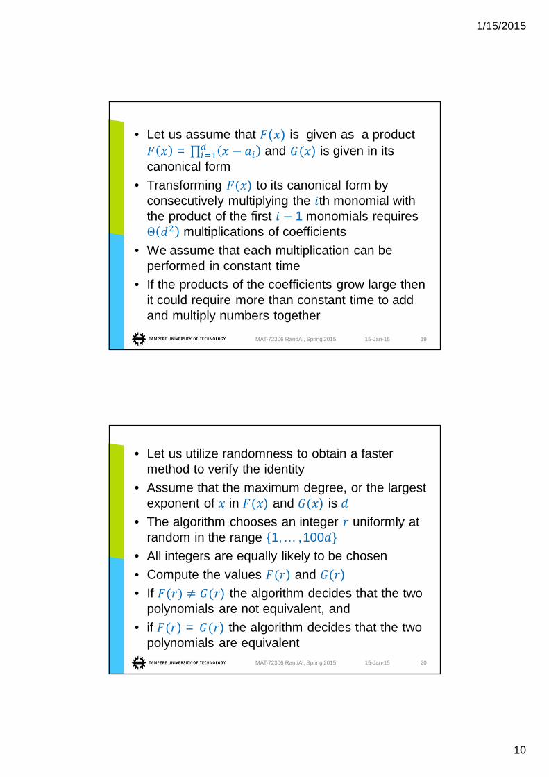
• Let us assume that ( ) is given as a product= and ) is given in its

canonical form• Transforming ) to its canonical form by

consecutively multiplying the th monomial withthe product of the first 1 monomials requires

multiplications of coefficients• We assume that each multiplication can be

performed in constant time• If the products of the coefficients grow large then

it could require more than constant time to addand multiply numbers together


• Let us utilize randomness to obtain a fastermethod to verify the identity

• Assume that the maximum degree, or the largestexponent of in ) and ) is

• The algorithm chooses an integer uniformly atrandom in the range {1, … , 100 }

• All integers are equally likely to be chosen• Compute the values ) and )• If ) the algorithm decides that the two

polynomials are not equivalent, and• if ) = ) the algorithm decides that the two

polynomials are equivalent15-Jan-15MAT-72306 RandAl, Spring 2015 20

1/15/2015

11

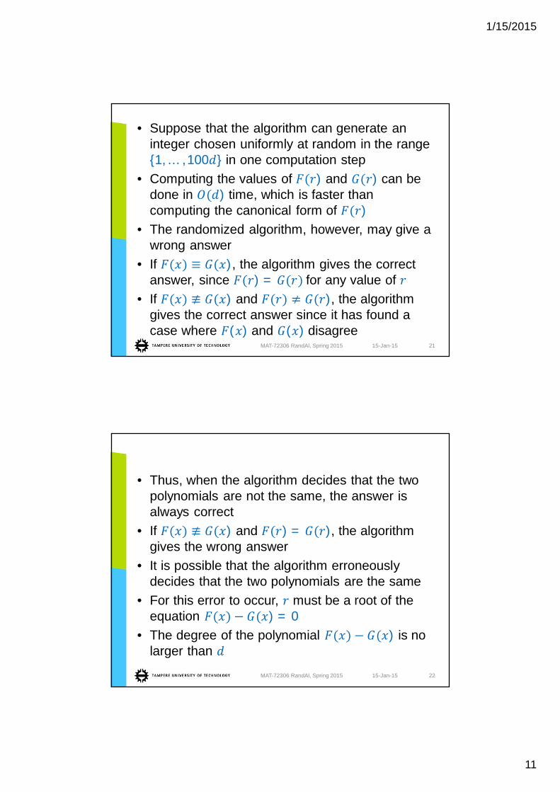
• Suppose that the algorithm can generate aninteger chosen uniformly at random in the range{1, … , 100 } in one computation step

• Computing the values of ) and ) can bedone in ) time, which is faster thancomputing the canonical form of )

• The randomized algorithm, however, may give awrong answer

• If ), the algorithm gives the correctanswer, since ) = for any value of

• If ) and ), the algorithmgives the correct answer since it has found acase where ( ) and ( ) disagree


• Thus, when the algorithm decides that the twopolynomials are not the same, the answer isalways correct

• If ) and ) = ), the algorithmgives the wrong answer

• It is possible that the algorithm erroneouslydecides that the two polynomials are the same

• For this error to occur, must be a root of theequation ) = 0

• The degree of the polynomial ) is nolarger than


1/15/2015

12

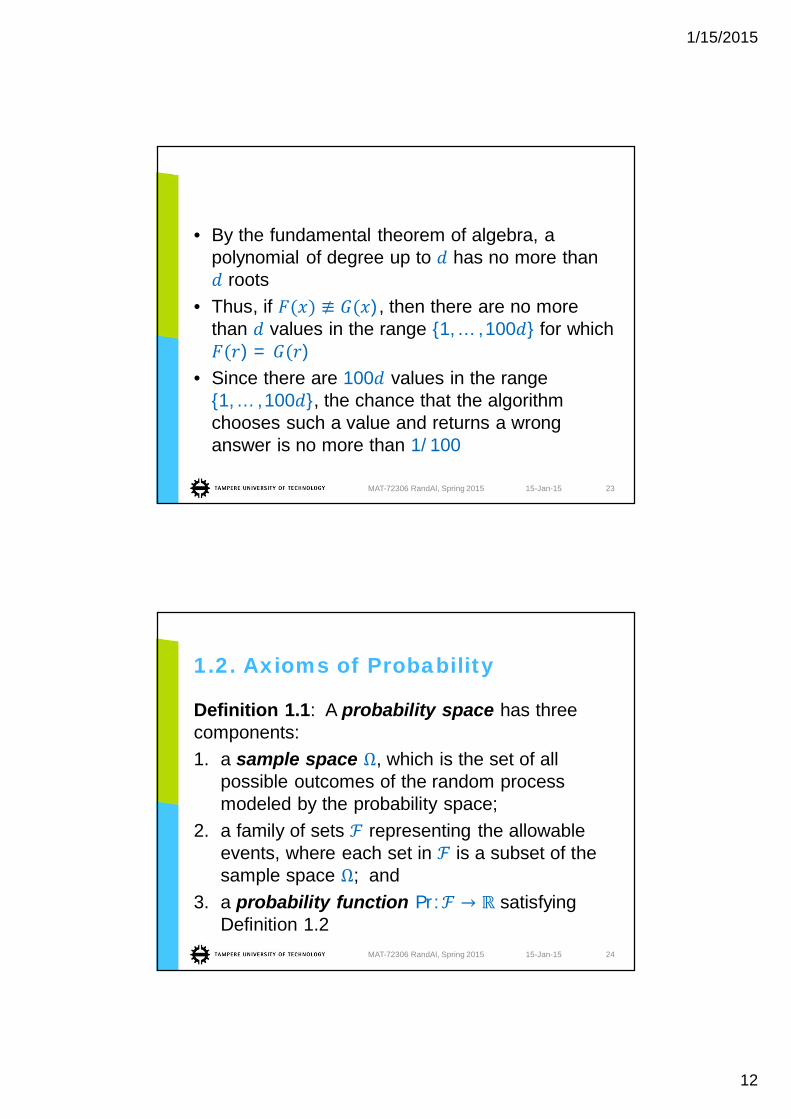
• By the fundamental theorem of algebra, apolynomial of degree up to has no more than

roots• Thus, if ), then there are no more

than values in the range {1, … , 100 } for which) = )

• Since there are 100 values in the range{1, … , 100 }, the chance that the algorithmchooses such a value and returns a wronganswer is no more than 1/100


1.2. Axioms of Probability

Definition 1.1: A probability space has threecomponents:1. a sample space , which is the set of all

possible outcomes of the random processmodeled by the probability space;

2. a family of sets representing the allowableevents, where each set in is a subset of thesample space ; and

3. a probability function Pr: satisfyingDefinition 1.2


1/15/2015

13

• An element of is called a simple orelementary event

• In the randomized algorithm for verifyingpolynomial identities, the sample space is theset of integers {1, … , 100 }

• Each choice of an integer in this range is asimple event


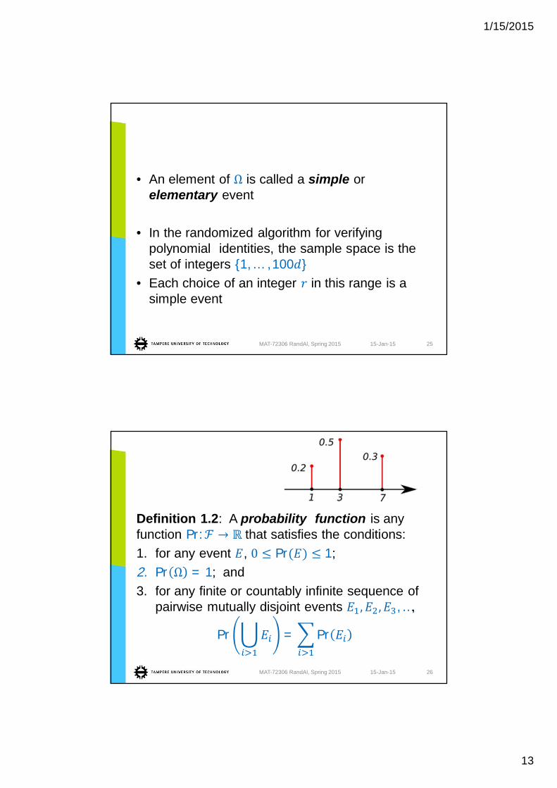
Definition 1.2: A probability function is anyfunction Pr: that satisfies the conditions:1. for any event , Pr 1;2. Pr = 1; and3. for any finite or countably infinite sequence of

pairwise mutually disjoint events , …,

Pr = Pr


1/15/2015

14

• We will mostly use discrete probability spaces• In a discrete probability space the sample space

is finite or countably infinite, and the familyof allowable events consists of all subsets of

• In a discrete probability space, the probabilityfunction is uniquely defined by the probabilitiesof the simple events

• Events are sets use standard set theorynotation to express combinations of events

• Write for the occurrence of both andand for the occurrence of either or(or both)


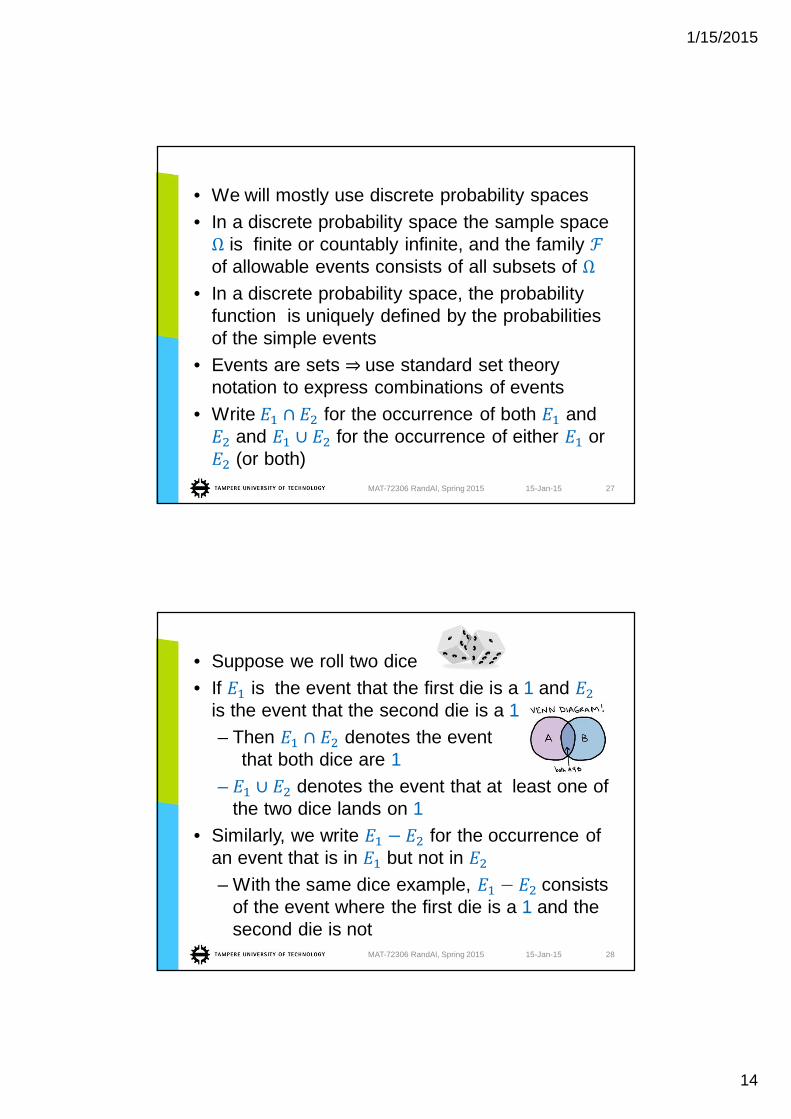
• Suppose we roll two dice• If is the event that the first die is a 1 and

is the event that the second die is a 1– Then denotes the event

that both dice are 1– denotes the event that at least one of

the two dice lands on 1• Similarly, we write for the occurrence of

an event that is in but not in– With the same dice example, consists

of the event where the first die is a 1 and thesecond die is not


1/15/2015

15

• We use the notation as shorthand for• E.g., if is the event that we obtain an even

number when rolling a die, then is the eventthat we obtain an odd number

• Definition 1.2 yields the following lemma

Lemma 1.1: For any two events and ,Pr = Pr + Pr Pr

• A consequence of Definition 2 is known as theunion bound


Lemma 1.2: For any finite or countably infinitesequence of events , …,

Pr Pr

• The third part of Definition 1.2 is an equality andrequires the events to be pairwise mutuallydisjoint


1/15/2015

16

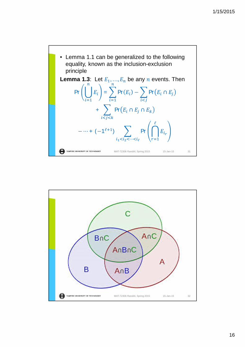
• Lemma 1.1 can be generalized to the followingequality, known as the inclusion-exclusionprinciple

Lemma 1.3: Let , … , be any events. Then

Pr = Pr Pr

+ Pr

+ ( 1 ) Pr



1/15/2015

17

• We showed that the only case in which thealgorithm may fail to give the correct answer iswhen the two polynomials ) and ) are notequivalent

• The algorithm then gives an incorrect answer ifthe random number it chooses is a root of thepolynomial )

• Let represent the event that the algorithmfailed to give the correct answer


• The elements of the set corresponding to arethe roots of the polynomial ) that arein the set of integers {1, … , 100 }

• Since the polynomial has no more than rootsit follows that the event includes no more than

simple events, and therefore

Pr algorithm fails = Pr =100

=1

100


1/15/2015

18

• The algorithm gives the correct answer 99% ofthe time even when the polynomials are notequivalent

• One way to improve this probability is to choosethe random number from a larger range ofintegers

• If our sample space is the set of integers{1, … , 1000 }, then the probability of a wronganswer is at most 1/1000

• At some point, however, the range of values wecan use is limited by the precision available onthe machine on which we run the algorithm


• Another approach is to repeat multiple times,using different random values to test the identity

• The algorithm has a one-sided error– It may be wrong only when it outputs that the two

polynomials are equivalent• If any run yields a number s.t. ),

then the polynomials are not equivalent• Repeat the algorithm a number of times and if

we find in any round, we know thatand ) are not equivalent

• Output that the two polynomials are equivalentonly if there is equality for all runs


1/15/2015

19

• In repeating the algorithm we repeatedly choosea random number in the range {1, … , 100 }

• Repeatedly choosing random numbers by agiven distribution is known as sampling

• We can repeatedly choose random numberseither with or without replacement– In sampling with replacement we do not

remember which numbers we have alreadytested

– Sampling without replacement means that,once we have chosen a number , we do notallow it to be chosen on subsequent runs


• Consider sampling with replacement• Assume that we repeat the algorithm times,

and that the input polynomials are not equivalent• What is the probability that in all iterations our

random sampling yields roots of the polynomial), resulting in a wrong output?

– If = 1: this probability is /100 = 1/100– If = 2, the probability that the 1st iteration finds

a root is 1/100 and the probability that the 2nd

iteration finds a root is 1/100, so the probabilitythat both iterations find a root is 1 100

• Generalizing, the probability of choosing rootsfor iterations would be 1 100


1/15/2015

20

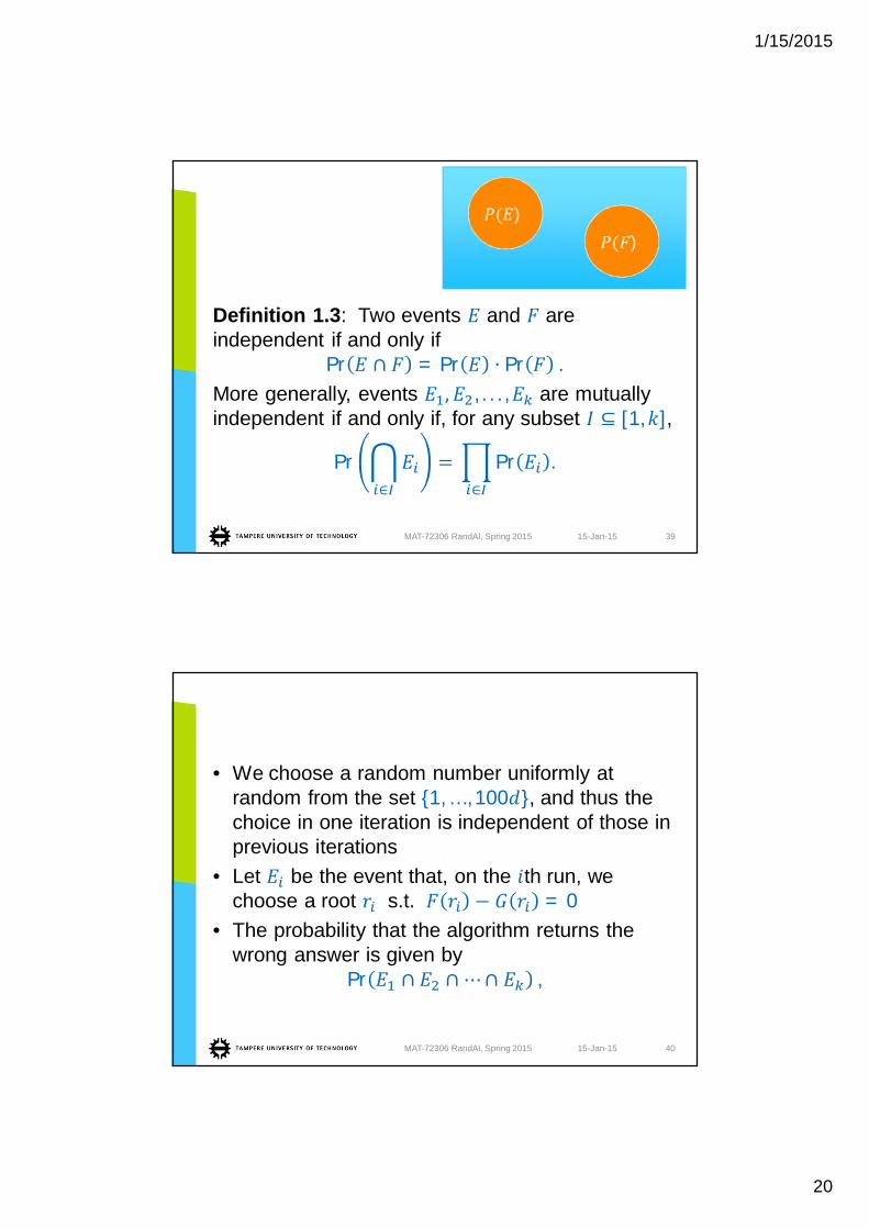
Definition 1.3: Two events and areindependent if and only if

Pr = Pr Pr .More generally, events , . . . , are mutuallyindependent if and only if, for any subset [1, ],

Pr Pr .


))))

• We choose a random number uniformly atrandom from the set {1, … , 100 }, and thus thechoice in one iteration is independent of those inprevious iterations

• Let be the event that, on the th run, wechoose a root s.t. = 0

• The probability that the algorithm returns thewrong answer is given by

Pr ,


1/15/2015

21

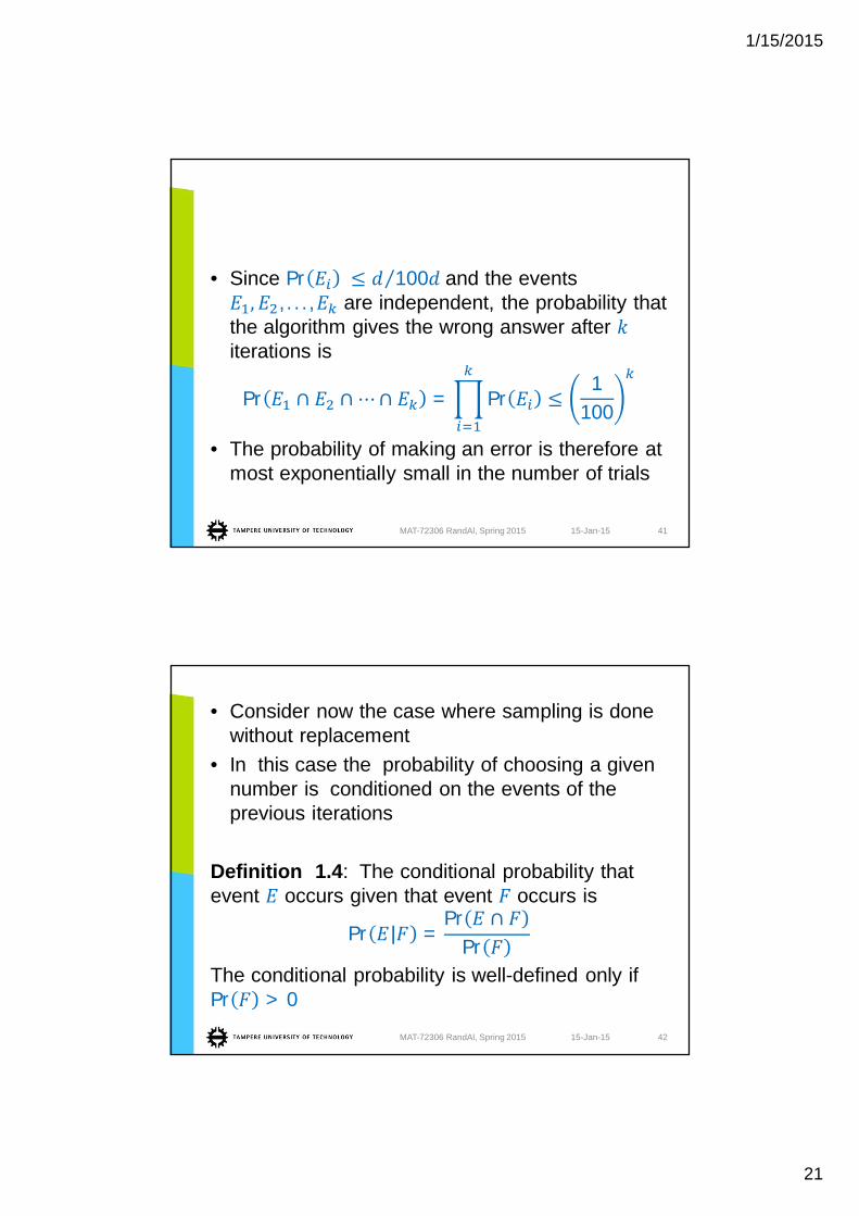
• Since Pr 100 and the events, . . . , are independent, the probability that

the algorithm gives the wrong answer afteriterations is

Pr = Pr1

100

• The probability of making an error is therefore atmost exponentially small in the number of trials


• Consider now the case where sampling is donewithout replacement

• In this case the probability of choosing a givennumber is conditioned on the events of theprevious iterations

Definition 1.4: The conditional probability thatevent occurs given that event occurs is

Pr =Pr

PrThe conditional probability is well-defined only ifPr > 0


1/15/2015

22


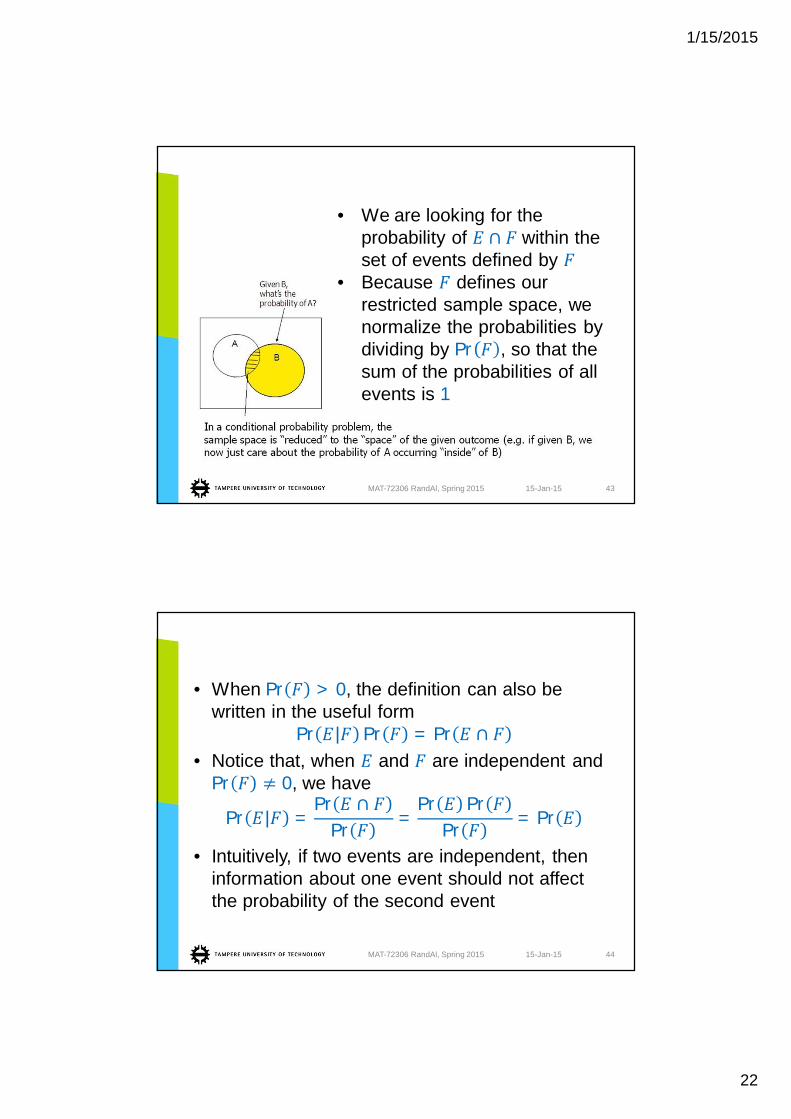
• We are looking for theprobability of within theset of events defined by

• Because defines ourrestricted sample space, wenormalize the probabilities bydividing by Pr , so that thesum of the probabilities of allevents is 1

• When Pr > 0, the definition can also bewritten in the useful form

Pr Pr = Pr• Notice that, when and are independent and

Pr 0, we have

Pr =Pr

Pr=

Pr PrPr

= Pr

• Intuitively, if two events are independent, theninformation about one event should not affectthe probability of the second event


1/15/2015

23

• What is the probability that in all the iterationsour random sampling without replacement yieldsroots of the polynomial ), resulting ina wrong output?

• As in the previous analysis, let be the eventthat the random number chosen in the thiteration of the algorithm is a root of )

• Again, the probability that the algorithm returnsthe wrong answer is given by

Pr


• Applying the definition of conditional probability,we obtain

Pr = PrPr

• Repeating this argument givesPr = Pr PrPr Pr

• Recall that there are at most values forwhich = 0


1/15/2015

24

• If trials 1 through 1 < have found 1 ofthem, then when sampling without replacementthere are only 1) values out of the100 1) remaining root choices

• Hence

Pr1)

100 1)• and the probability of the wrong answer after

iterations is bounded by

Pr1)

100 1)1

100


• ( ( 1))/(100 ( 1)) < /100 when> 1, and our bounds on the probability of an

error are actually slightly better withoutreplacement

• Also, if we take + 1 samples w/o replacementand two polynomials are not equivalent, then weare guaranteed to find an s.t. 0

• Thus, in + 1 iterations we are guaranteed tooutput the correct answer

• However, computing the value of the polynomialat + 1 points takes ) time using thestandard approach, which is no faster thanfinding the canonical form deterministically


1/15/2015

25

1.3. Verifying Matrix Multiplication

• We are given three matrices A, B, and• For convenience, assume we are working over

the integers modulo 2• We want to verify whether

AB = C• One way to accomplish this is to multiply A and

B and compare the result to• The simple matrix multiplication algorithm takes

) operations


• We use a randomized algorithm that allows forfaster verification – at the expense of possiblyreturning a wrong answer with small probability

• It is similar in spirit to our randomized algorithmfor checking polynomial identities

• The algorithm chooses a random vector= ( , … , 0,1

• It then computes by first computing andthen ), and it also computes

• If , then AB C• Otherwise, it returns that AB = C


1/15/2015

26

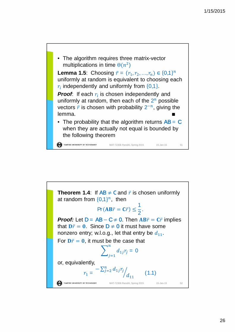
• The algorithm requires three matrix-vectormultiplications in time )

Lemma 1.5: Choosing = ( , … , 0,1uniformly at random is equivalent to choosing each

independently and uniformly from 0,1 .Proof: If each is chosen independently anduniformly at random, then each of the 2 possiblevectors is chosen with probability 2 , giving thelemma.• The probability that the algorithm returns AB = C

when they are actually not equal is bounded bythe following theorem


Theorem 1.4: If AB C and is chosen uniformlyat random from 0,1 , then

Pr12

.

Proof: Let D = AB C 0. Then impliesthat . Since D 0 it must have somenonzero entry; w.l.o.g., let that entry be .For , it must be the case that

= 0

or, equivalently,

= (1.1)


1/15/2015

27

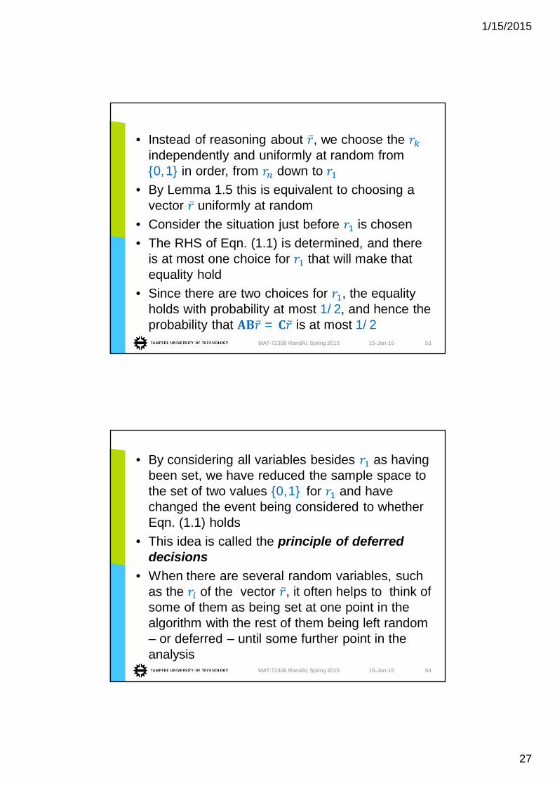
• Instead of reasoning about , we choose theindependently and uniformly at random from{0, 1} in order, from down to

• By Lemma 1.5 this is equivalent to choosing avector uniformly at random

• Consider the situation just before is chosen• The RHS of Eqn. (1.1) is determined, and there

is at most one choice for that will make thatequality hold

• Since there are two choices for , the equalityholds with probability at most 1/2, and hence theprobability that = is at most 1/2


• By considering all variables besides as havingbeen set, we have reduced the sample space tothe set of two values {0, 1} for and havechanged the event being considered to whetherEqn. (1.1) holds

• This idea is called the principle of deferreddecisions

• When there are several random variables, suchas the of the vector , it often helps to think ofsome of them as being set at one point in thealgorithm with the rest of them being left random– or deferred – until some further point in theanalysis


1/15/2015

28

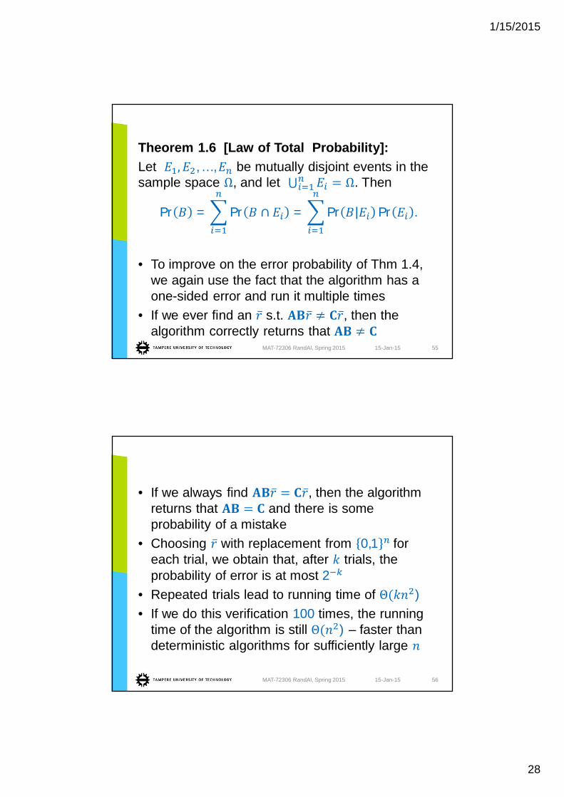
Theorem 1.6 [Law of Total Probability]:Let , … , be mutually disjoint events in thesample space , and let . Then

Pr = Pr = Pr Pr .

• To improve on the error probability of Thm 1.4,we again use the fact that the algorithm has aone-sided error and run it multiple times

• If we ever find an s.t. , then thealgorithm correctly returns that


• If we always find , then the algorithmreturns that and there is someprobability of a mistake

• Choosing with replacement from 0,1 foreach trial, we obtain that, after trials, theprobability of error is at most 2

• Repeated trials lead to running time of )• If we do this verification 100 times, the running

time of the algorithm is still ) – faster thandeterministic algorithms for sufficiently large


1/15/2015

29

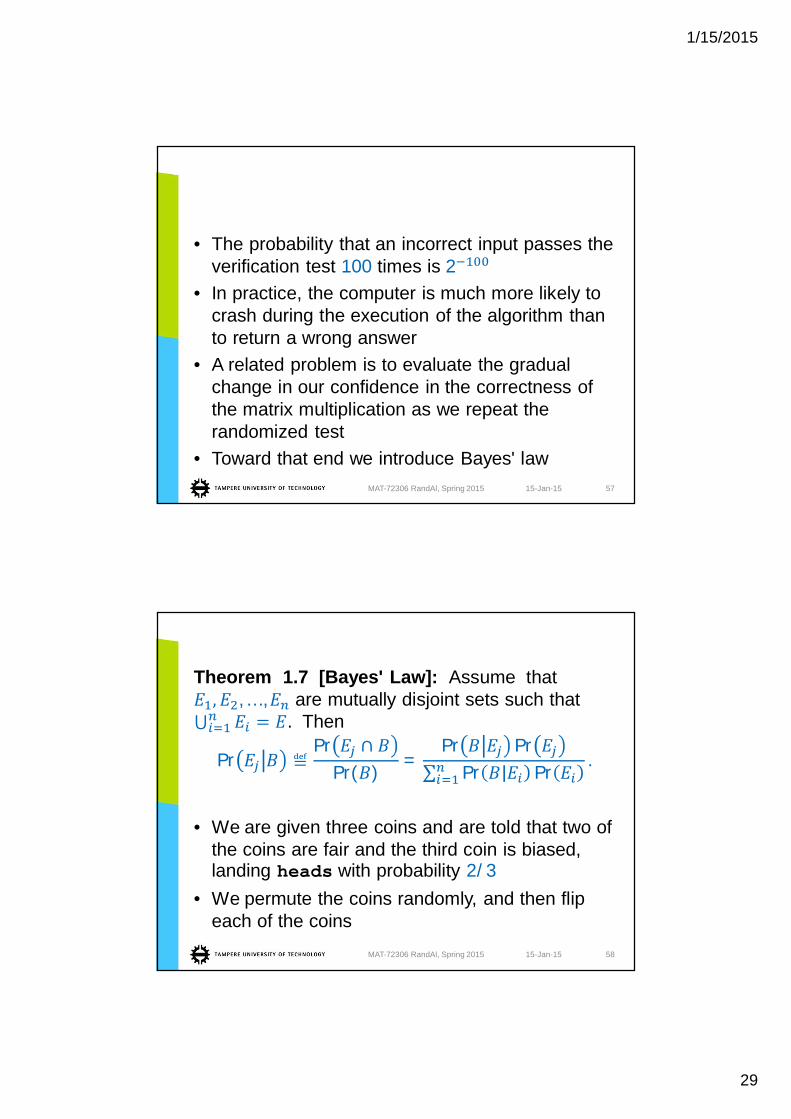
• The probability that an incorrect input passes theverification test 100 times is 2

• In practice, the computer is much more likely tocrash during the execution of the algorithm thanto return a wrong answer

• A related problem is to evaluate the gradualchange in our confidence in the correctness ofthe matrix multiplication as we repeat therandomized test

• Toward that end we introduce Bayes' law15-Jan-15MAT-72306 RandAl, Spring 2015 57

Theorem 1.7 [Bayes' Law]: Assume that, … , are mutually disjoint sets such that

. Then

PrPr

Pr( )=

Pr PrPr Pr

.

• We are given three coins and are told that two ofthe coins are fair and the third coin is biased,landing heads with probability 2/3

• We permute the coins randomly, and then flipeach of the coins


1/15/2015

30

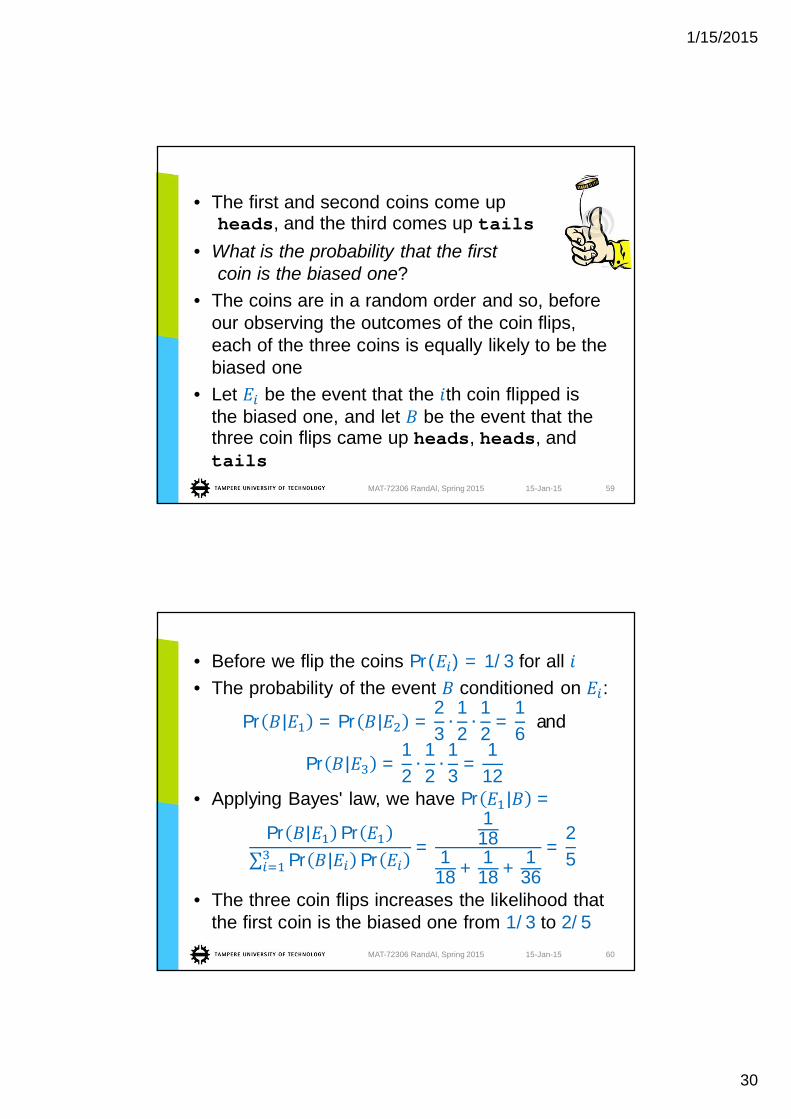
• The first and second coins come upheads, and the third comes up tails

• What is the probability that the firstcoin is the biased one?

• The coins are in a random order and so, beforeour observing the outcomes of the coin flips,each of the three coins is equally likely to be thebiased one

• Let be the event that the th coin flipped isthe biased one, and let be the event that thethree coin flips came up heads, heads, andtails


• Before we flip the coins Pr( ) = 1/3 for all• The probability of the event conditioned on :

Pr = Pr =23

12

12

=16

and

Pr =12

12

13

=1

12• Applying Bayes' law, we have Pr =

Pr PrPr Pr

=1

181

18 + 118 + 1

36=

25

• The three coin flips increases the likelihood thatthe first coin is the biased one from 1/3 to 2/5


1/15/2015

31

• In randomized matrix multiplication test, we wantto evaluate the increase in confidence in thematrix identity obtained through repeated tests

• In the Bayesian approach one starts with a priormodel, giving some initial value to the modelparameters

• This model is then modified, by incorporatingnew observations, to obtain a posterior modelthat captures the new information

• If we have no information about the process thatgenerated the identity then a reasonable priorassumption is that the identity is correct withprobability 1/2


• Let be the event that the identity is correct,and let be the event that the test returns thatthe identity is correct

• We start with Pr = Pr = 1 2, and sincethe test has a one-sided error bounded by 1 2,we have Pr = 1 and Pr 1 2

• Applying Bayes' law yields

Pr =Pr Pr

Pr Pr + Pr Pr1 2

1 2 + 1 2 1 2=

23


1/15/2015

32

• Assume now that we run the randomized testagain and it again returns that the identity iscorrect

• After the first test, we may have revised our priormodel, so that we believe Pr 2/3 andPr 1/3

• Now let be the event that the new test returnsthat the identity is correct; since the tests areindependent, as before we have

Pr = 1 and Pr 1/2


• Applying Bayes' law then yields

Pr2 3

2 3 + 1 3 1 2=

45

• In general: If our prior model (before running thetest) is that Pr 2 2 + 1 and if the testreturns that the identity is correct (event ), then

Pr =2

2 + 1= 1

12 + 1

• Thus, if all 100 calls to the matrix identity testreturn that it is correct, our confidence in thecorrectness of this identity is 1/(2 + 1)


1/15/2015

33

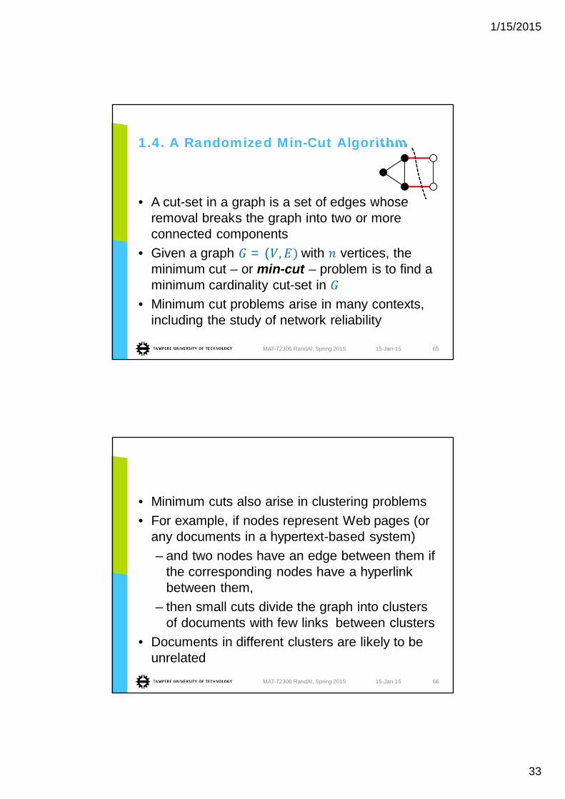
1.4. A Randomized Min-Cut Algorithm

• A cut-set in a graph is a set of edges whoseremoval breaks the graph into two or moreconnected components

• Given a graph = ( with vertices, theminimum cut – or min-cut – problem is to find aminimum cardinality cut-set in

• Minimum cut problems arise in many contexts,including the study of network reliability


• Minimum cuts also arise in clustering problems• For example, if nodes represent Web pages (or

any documents in a hypertext-based system)– and two nodes have an edge between them if

the corresponding nodes have a hyperlinkbetween them,

– then small cuts divide the graph into clustersof documents with few links between clusters

• Documents in different clusters are likely to beunrelated


1/15/2015

34

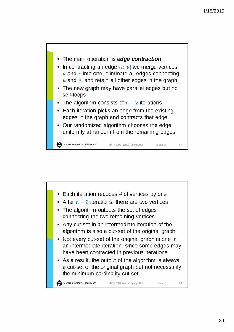
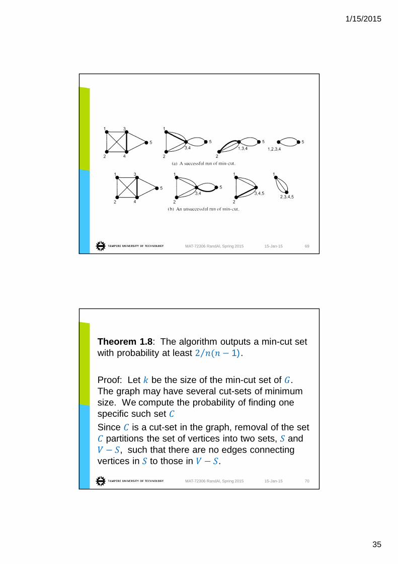
• The main operation is edge contraction• In contracting an edge we merge vertices

and into one, eliminate all edges connectingand , and retain all other edges in the graph

• The new graph may have parallel edges but noself-loops

• The algorithm consists of 2 iterations• Each iteration picks an edge from the existing

edges in the graph and contracts that edge• Our randomized algorithm chooses the edge

uniformly at random from the remaining edges


• Each iteration reduces # of vertices by one• After 2 iterations, there are two vertices• The algorithm outputs the set of edges

connecting the two remaining vertices• Any cut-set in an intermediate iteration of the

algorithm is also a cut-set of the original graph• Not every cut-set of the original graph is one in

an intermediate iteration, since some edges mayhave been contracted in previous iterations

• As a result, the output of the algorithm is alwaysa cut-set of the original graph but not necessarilythe minimum cardinality cut-set


1/15/2015

35


Theorem 1.8: The algorithm outputs a min-cut setwith probability at least 1).

Proof: Let be the size of the min-cut set of .The graph may have several cut-sets of minimumsize. We compute the probability of finding onespecific such setSince is a cut-set in the graph, removal of the set

partitions the set of vertices into two sets, and, such that there are no edges connecting

vertices in to those in .


1/15/2015

36

Assume that, throughout an execution of thealgorithm, we contract only edges that connect twovertices in or two in , but not edges in .In that case, all the edges eliminated throughoutthe execution will be edges connecting vertices in

or vertices in , and after 2 iterations thealgorithm returns a graph with two verticesconnected by the edges in .We may conclude that, if the algorithm neverchooses an edge of in its 2 iterations, thenthe algorithm returns as the minimum cut-set.


If the size of the cut is small, then the probabilitythat the algorithm chooses an edge of is small –at least when the number of edges remaining islarge compared to .Let be the event that the edge contracted initeration is not in , and let = be theevent that no edge of was contracted in the firstiterations. We need to compute Pr .Start by computing Pr = Pr . Since theminimum cut-set has edges, all vertices in thegraph must have degree or larger. If each vertexis adjacent to at least edges, then the graphmust have at least 2 edges.


1/15/2015

37

Since there are at least /2 edges in the graphand since has edges, the probability that wedo not choose an edge of in the first iteration is

Pr = Pr = 1 = 12

Suppose that the first contraction did not eliminatean edge of . I.e., we condition on the event .Then, after the first iteration, we are left with an

1)-node graph with minimum cut-set of size .Again, the degree of each vertex in the graph mustbe at least , and the graph must have at least

1)/2 edges.


Pr 11 2

= 12

1Similarly,

Pr+ 1 2

= 12

+ 1To compute Pr , we use

Pr = Pr= Pr Pr= Pr Pr Pr Pr

2+ 1

=1

+ 1

=2 3

124

13

=2

1.
