Random-Variate Generation

2

Purpose & Overview

Develop understanding of generating samples from a specified distribution as input to a simulation model.

Illustrate some widely-used techniques for generating random variates.Inverse-transform techniqueConvolution techniqueAcceptance-rejection techniqueA special technique for normal distribution

3

Inverse-transform Technique

The concept:For cdf function: r = F(x)Generate R sample from uniform (0,1) Find X sample:

X = F-1(R)

r1

x1

r = F(x)

1Pr( ) Pr( ( ) ) Pr( ( )) ( )X x F R x R F x F x

4

Exponential Distribution [Inverse-transform]

Exponential Distribution: Exponential cdf:

To generate X1, X2, X3 ,… generate R1, R2, R3 ,…

r = F(x) = 1 – e-x for x 0

Xi = F-1(Ri) = -(1/ ln(1-Ri)

Figure: Inverse-transform technique for exp( = 1)

5

Example: Generate 200 variates Xi with distribution exp(= 1)

Matlab Codefor i=1:200,

expnum(i)=-log(rand(1));

end

Exponential Distribution [Inverse-transform]

R and (1 – R) have U(0,1) distribution

6

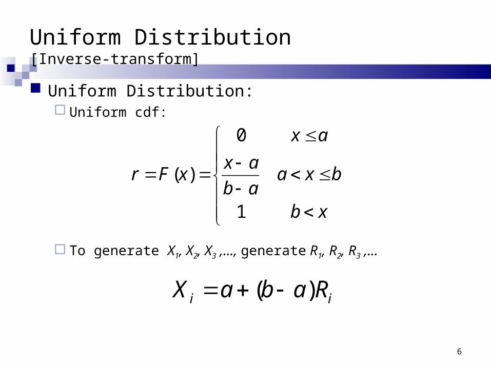
Uniform Distribution: Uniform cdf:

To generate X1, X2, X3 ,…, generate R1, R2, R3 ,…

Uniform Distribution [Inverse-transform]

0

( )

1

x a

x ar F x a x b

b ab x

( )i iX a b a R

7

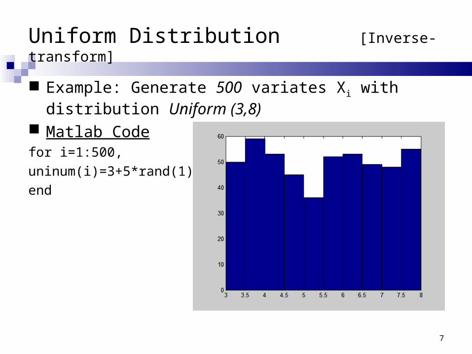
Example: Generate 500 variates Xi with distribution Uniform (3,8)

Matlab Codefor i=1:500,

uninum(i)=3+5*rand(1);

end

Uniform Distribution [Inverse-transform]

8

Discrete Distribution [Inverse-transform]

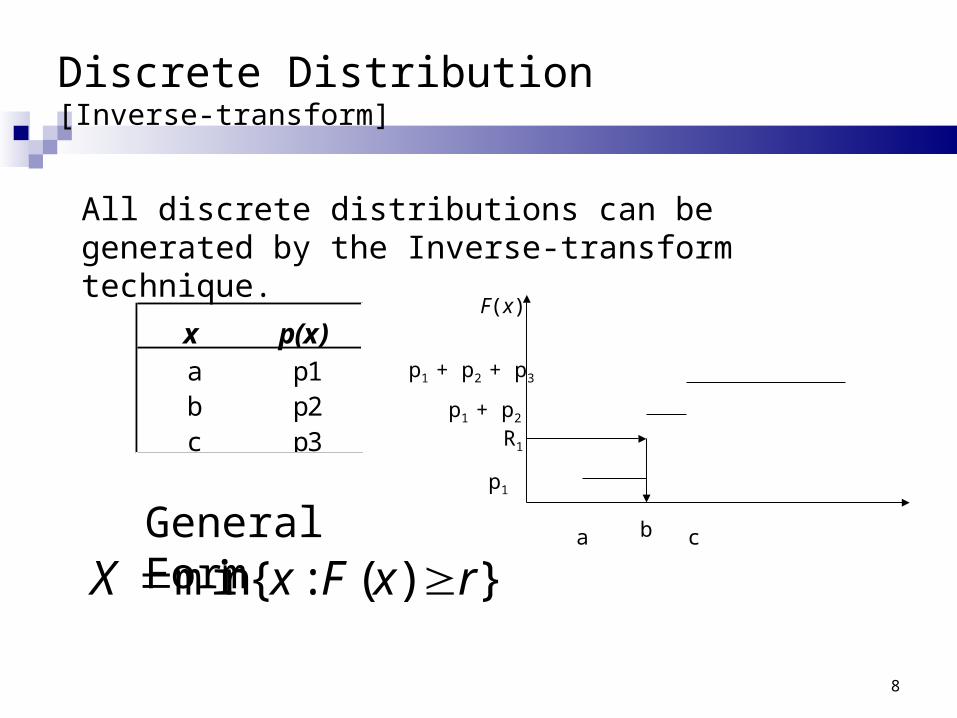
x p(x)a p1b p2c p3

All discrete distributions can be generated by the Inverse-transform technique.

p1

p1 + p2

p1 + p2 + p3

a b c

F(x)

R1

min{ : ( ) }X x F x r General Form

9

Discrete Distribution [Inverse-transform]

Example: Suppose the number of shipments, x, on the loading dock of IHW company is either 0, 1, or 2 Data - Probability distribution:

Method - Given R, the generation

scheme becomes:

0, 0.5

1, 0.5 0.8

2, 0.8 1.0

R

x R

R

Consider R 1 = 0.73:F(x i-1) < R <= F(x i)F(x 0) < 0.73 <= F(x 1)

Hence, x 1 = 1

x p(x) F(x)0 0.50 0.501 0.30 0.802 0.20 1.00

10

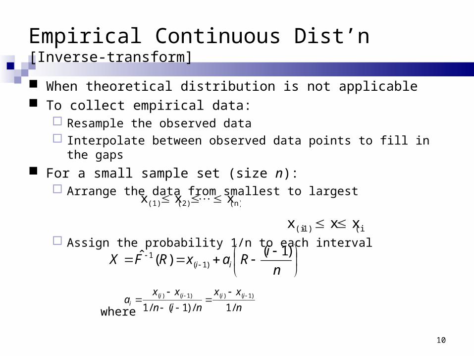
Empirical Continuous Dist’n [Inverse-transform]

When theoretical distribution is not applicable To collect empirical data:

Resample the observed data Interpolate between observed data points to fill in the gaps

For a small sample set (size n): Arrange the data from smallest to largest

Assign the probability 1/n to each interval

where

(n)(2)(1) x x x

(i)1)-(i x x x

n

iRaxRFX ii

)1()(ˆ

)1(1

n

xx

nin

xxa iiiii /1/)1(/1

)1()()1()(

11

Empirical Continuous Dist’n [Inverse-transform]

Example: Suppose the data collected for 100 broken-widget repair times are:

iInterval (Hours) Frequency

Relative Frequency

Cumulative Frequency, c i

Slope, a i

1 0.25 ≤ x ≤ 0.5 31 0.31 0.31 0.81

2 0.5 ≤ x ≤ 1.0 10 0.10 0.41 5.0

3 1.0 ≤ x ≤ 1.5 25 0.25 0.66 2.0

4 1.5 ≤ x ≤ 2.0 34 0.34 1.00 1.47

Consider R 1 = 0.83:

c 3 = 0.66 < R 1 < c 4 = 1.00

X 1 = x (4-1) + a 4(R 1 – c (4-1)) = 1.5 + 1.47(0.83-0.66) = 1.75

12

Convolution Technique

Use for X = Y1 + Y2 + … + Yn

Example of applicationErlang distribution

Generate samples for Y1 , Y2 , … , Yn and then add these samples to get a sample of X.

13

Example: Generate 500 variates Xi with distribution Erlang-3 (mean: k/

Matlab Codefor i=1:500,

erlnum(i)=-1/6*(log(rand(1))+log(rand(1))+log(rand(1)));

end

Erlang Distribution [Convolution]

14

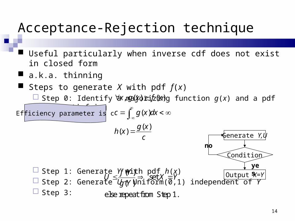
Useful particularly when inverse cdf does not exist in closed form a.k.a. thinning Steps to generate X with pdf f(x)

Step 0: Identify a majorizing function g(x) and a pdf h(x) satisfying

Step 1: Generate Y with pdf h(x) Step 2: Generate U ~ Uniform(0,1) independent of Y Step 3:

Acceptance-Rejection technique

, ( ) ( )

( )

( )( )

x g x f x

c g x dx

g xh x

c

Generate Y,U

Condition

Output X=Y

yes

no

( ) set

( )

else repeat from Step 1.

f YU X Y

g Y

Efficiency parameter is c

15

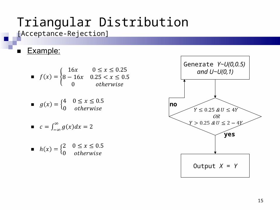
Triangular Distribution [Acceptance-Rejection]

Generate Y~U(0,0.5) and U~U(0,1)

Output X = Y

yes

no

16

Triangular Distribution [Acceptance-Rejection]

Matlab Code: (for exactly 1000 samples)i=0;while i<1000, Y=0.5*rand(1); U=rand(1); if Y<=0.25 & U<=4*Y | Y>0.25 & U<=2-4*Y i=i+1; X(i)=Y; endend

0 0.05 0.1 0.15 0.2 0.25 0.3 0.35 0.4 0.45 0.50

20

40

60

80

100

120

140

160

180

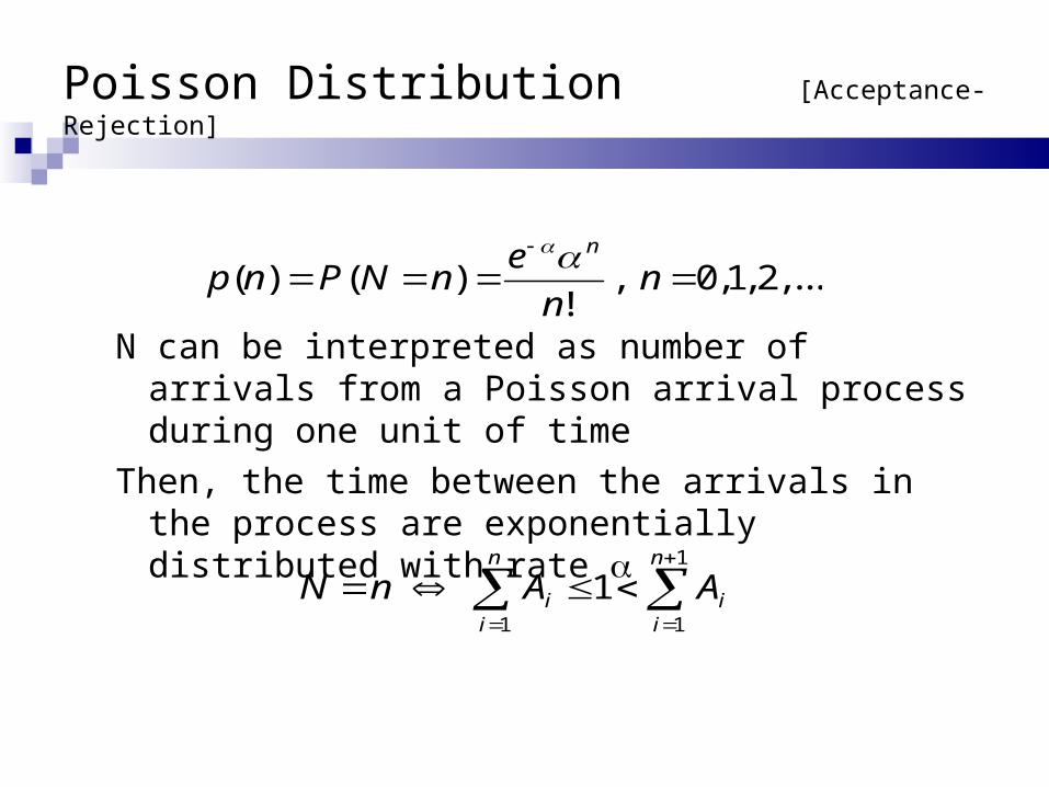
N can be interpreted as number of arrivals from a Poisson arrival process during one unit of time

Then, the time between the arrivals in the process are exponentially distributed with rate

...,2,1,0,!

)()(

nn

enNPnp

n

1

11

1n

ii

n

ii AAnN

Poisson Distribution [Acceptance-Rejection]

Step 1. Set n = 0, and P = 1

Step 2. Generate a random number Rn+1 and let P = P. Rn+1

Step 3. If P < e-, then accept N = n. Otherwise, reject current n, increase n by one, and return to step 2

How many random numbers will be used on the average to generate one Poisson variate?

1

11

1

11

1

11

ln1

1ln1

1

n

ii

n

ii

n

ii

n

ii

n

ii

n

ii

ReR

RRAA

Poisson Distribution [Acceptance-Rejection]

19

Approach for normal(0,1): Consider two standard normal random variables, Z1 and Z2,

plotted as a point in the plane:

B2 = Z21 + Z2

2 ~ chi-square distribution with 2 degrees of freedom = Exp( = 1/2). Hence,

The radius B and angle are mutually independent.

Normal Distribution [Special Technique]

2/1)ln2( RB

In polar coordinates:Z1 = B cos Z2 = B sin

1/ 21 1 2

1/ 22 1 2

( 2 ln ) cos(2 )

( 2 ln ) sin(2 )

Z R R

Z R R

Uniform(0,2

20

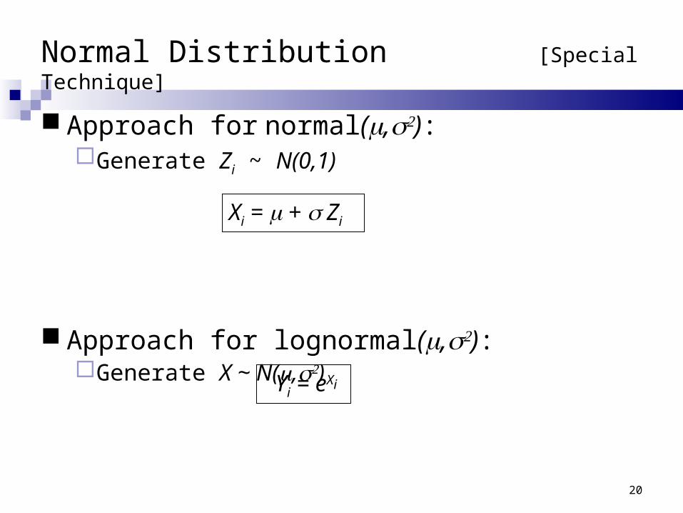
Normal Distribution [Special Technique]

Approach for normal(,):Generate Zi ~ N(0,1)

Approach for lognormal(,):Generate X ~ N(,) Yi = eXi

Xi = + Zi

21

Normal Distribution [Special Technique]

Generate 1000 samples of Normal(7,4) Matlab Codefor i=1:500, R1=rand(1); R2=rand(1); Z(2*i-1)=sqrt(-2*log(R1))*cos(2*pi*R2); Z(2*i)=sqrt(-2*log(R1))*sin(2*pi*R2);end

for i=1:1000, Z(i)=7+2*Z(i);end