Chapter 5

1

Random Variables and Probability Distributions

Random Variables

• Definition:– A rule that assigns one (and only one)

numerical value to each simple event of an experiment; or

– A function that assigns numerical values to the possible outcomes of an experiment.

• Two types:– Discrete– Continuous

Discrete Random Variables

• Definition:– A random variable whose numerical values are

limited to specific values within its range; or

– A random variable that can assume a countable number of values.

• Examples: – number of traffic accidents

– mortgage rates

– shoe size

Continuous Random Variables

• Definition:– A random variable that can take any value over a

continuous range of values; or– A random variable that can assume values

corresponding to any of the points contained in one or more intervals.

• Example:– length of right foot of a person– length of time between arrivals– weight of a food item bought at a store

Chapter 5

2

Examples

• Are the following discrete or continuous random variables?– The pump price of a gallon of gasoline in

dollars.– The time taken by a flight from New York to

London.– The age of a grocery store shopper in years.

Probability Distribution for a Discrete Random Variable

• Definition:– A list of all the possible values of the random variable

and their respective probabilities; or

– A graph, table or formula that specifies the probability associated with each possible value the random variable can assume.

• Requirements:– 1. for all values of x

– 2. 1)(1

iixp

0)( ixp

Example

• Let the random variable of interest be the face value shown when tossing a die:– For x=1, P(x)=1/6,

– For x=2, P(x)=1/6,

– For x=3, P(x)=1/6,

– For x=4, P(x)=1/6,

– For x=5, P(x)=1/6,

– For x=6, P(x)=1/6.

p x( ) 0

p xx

( ) 1

Example

• Let the random variable of interest be the number of heads observed when two fair coins are tossed:– {No heads observed} For x=0,

P(x=0)=P(T1,T2)=1/4– {One head observed} For x=1,

P(x=1)=P(T1,H2)+P(H1,T2)=1/4+1/4=1/2– {Two heads observed} For x=2,

P(x=2)=P(H1,H2)=1/4

Chapter 5

3

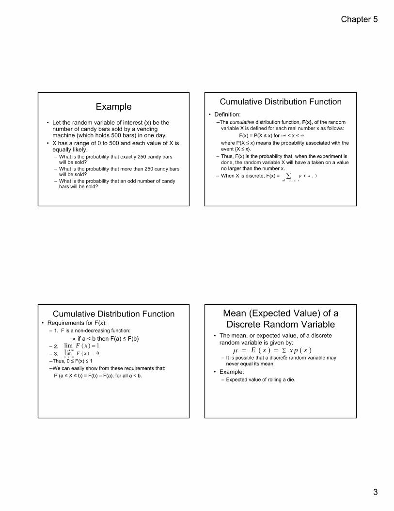
Example

• Let the random variable of interest (x) be the number of candy bars sold by a vending machine (which holds 500 bars) in one day.

• X has a range of 0 to 500 and each value of X is equally likely.– What is the probability that exactly 250 candy bars

will be sold?– What is the probability that more than 250 candy bars

will be sold?– What is the probability that an odd number of candy

bars will be sold?

Cumulative Distribution Function

• Definition:--The cumulative distribution function, F(x), of the random

variable X is defined for each real number x as follows:

F(x) = P(X ≤ x) for -∞ < x < ∞

where P(X ≤ x) means the probability associated with the event {X ≤ x}.

– Thus, F(x) is the probability that, when the experiment is done, the random variable X will have a taken on a value no larger than the number x.

– When X is discrete, F(x) = xxall

i

i

xp )(

Cumulative Distribution Function• Requirements for F(x):

– 1. F is a non-decreasing function:

» if a < b then F(a) ≤ F(b)– 2.

– 3.

--Thus, 0 ≤ F(x) ≤ 1

--We can easily show from these requirements that:

P (a ≤ X ≤ b) = F(b) – F(a), for all a < b.

1)(lim

xFx

0)(lim

xFx

Mean (Expected Value) of a Discrete Random Variable

• The mean, or expected value, of a discrete random variable is given by:

– It is possible that a discrete random variable may never equal its mean.

• Example:– Expected value of rolling a die.

E x x p xx

( ) ( )

Chapter 5

4

Example

• From earlier die toss experiment:– x=1, P(x)=1/6, - x=4, P(x)=1/6,

– x=2, P(x)=1/6, - x=5, P(x)=1/6,

– x=3, P(x)=1/6, - x=6, P(x)=1/6.

• Mean or expected value:

5.3)6

1*6()

6

1*5()

6

1*4()

6

1*3()

6

1*2()

6

1*1(

)()(

x

xxpxE

Variance of a Discrete Random Variable

• The variance of a discrete random variable is given by:

• Examples:– Variance of rolling a die.

• Standard deviation is the positive square root of the variance.

2 2 2 E x x p xx

[( ) ] ( ) ( )

Example

• From earlier die toss experiment:– x=1, P(x)=1/6; x=2, P(x)=1/6; x=3, P(x)=1/6; x=4,

P(x)=1/6; x=5, P(x)=1/6; x=6, P(x)=1/6.

– E(x)=3.5

• Variance:

9167.2)6

1*)5.36(()

6

1*)5.35(()

6

1*)5.34((

)6

1*)5.33(()

6

1*)5.32(()

6

1*)5.31((

)()(])[(

222

222

222

x

xpxxE

Other Related Topics• Excel’s RAND() function generates a number

between 0 and 1.

• When two random variables are related in the sense that they both depend on which of several possible scenarios occurs, the covariance and correlationare summary measures of the relationship between them.

• p(xi, yi), the joint probability,is the probability that the random variables X and Y equal the values xi

and yi, respectively.

• When X and Y are independent random variables, the joint probability is equal to the product of the marginals.

Chapter 5

5

Binomial Random Variable

• Definition:– The random variable (x) which represents the

number of successes that occur in n independent trials is said to be a binomial random variable with parameters (n,p) where p is the probability of success on a given trial.

– Counts the number of successes (or failures) in n trials.

Characteristics of a Binomial Random Variable

• The experiment consists of n identical trials.

• There are only two possible outcomes on each trial (S for Success or F for Failure).

• The probability of a success (S) is p for each trial. P(S)= p; P(F)= q; p+q=1.

• The trials are independent.

• The binomial random variable x is the number of Successes in n independent trials.

Example

• Flip a coin 50 times. Count the number of heads.

• A type of machine breaks down 10% of the time on a production run. Count the breakdowns in 60 production runs.

• Some customers purchase gum when checking out at a store. Count the number of customers who purchase gum.

Binomial Probability Distribution

• where – p=probability of a success on a single trial– q=1-p– n=Number of trials– x=Number of successes in n trials

p xn

xp q

x n

x n x( )

( , , , , . . . . , )

0 1 2 3

Chapter 5

6

p xn

xp q

x n

x n x( )

( , , , , . . . . , )

0 1 2 3

xnx qp

x

n

Binomial Probability Distribution

Number of simple events n with x Successes….

Probability of x Successes and (n-x) Failures in

any simple event….

Example

• Toss four coins:– What is the probability of obtaining two heads

and two tails?

– What is the probability of obtaining one head and three tails?

375.0)5.0()5.0()!24(!2

!4

)5.0()5.0(2

4)2(

242

242

p

250.0)5.0()5.0()!14(!1

!4

)5.0()5.0(1

4)1(

141

141

p

Example

• A machine produces defective items with a probability of 0.1:– What is the probability that in a sample of five items,

at most one item will be defective?

– What is the probability that in a sample of five items, exactly two items will be defective?

– What is the probability that in a sample of five items, more than three items will be defective?

Example

• Let x be the number of defective items out of five:

00001.0)9.0()1.0(5

5)5(

00045.0)9.0()1.0(4

5)4(

00810.0)9.0()1.0(3

5)3(

07290.0)9.0()1.0(2

5)2(

32805.0)9.0()1.0(1

5)1(

59049.0)9.0()1.0(0

5)0(

555

454

353

252

151

050

p

p

p

p

p

p

Chapter 5

7

Example

– What is the probability that in a sample of five items, at most one item will be defective?

– What is the probability that in a sample of five items, exactly two items will be defective?

– What is the probability that in a sample of five items, more than three items will be defective?

91854.032805.059049.0)1()0()1( xpxpxp

07290.0)2( xp

00046.000001.000045.0)5()4()3( xpxpxp

Mean, Variance, Standard Deviation of a Binomial Random Variable

• Mean:

• Variance:

• Standard Deviation:

2 n p q

n p q

E x n p( )

Example

• Let x be a binomial random variable with p=0.7 and n=10:– The mean is:

– The variance is:

– The standard deviation is:

0.77.0*10)( npxE

1.23.0*7.0*102

449.11.23.0*7.0*10 npq

Binomial Example

• Experiment:– Flip a coin three times and record the value of

the up face.– What is the probability of getting exactly two

heads?– Eight possible sequences of heads and tails

(why?). Xn=23=8– HHH, HHT, HTH, HTT, THH, THT, TTH, TTT.

Chapter 5

8

Example

• Each sequence is equally likely, that is p(x)=1/8=0.125:– How many ways to get 2 heads?

– Probability of each sequence is:

– Probability of exactly two heads is 3 out of 8 (3/8=0.375) by counting or (3*0.125=0.375) by binomial formula.

32

2*3

!2

!3

)!23(!2

!3

2

3

x

N

125.0)5.0()5.0( 12)( xnxqp

Probability Table

• A table that lists the probability of any two characteristics where each characteristic can take on multiple values.

• Example:

– Grocery shoppers by gender and senior citizen status.

Male FemaleSenior Citizen 0.02 0.08 0.10Not Senior Citizen 0.28 0.62 0.90

0.30 0.70 1.00

Continuous Random Variables

• f(x) is the probability density function of the continuous random variable x if these conditions are met for any values a and b:– 1.

– 2.

– 3.

f x( ) , 0 x

f x d x( )

1

P a X b f x d xa

b( ) ( )

Mean (Expected Value) for a Continuous Random Variable

• The expected value of a continuous random variable x is the average or mean value of x and is given by:

E X x f x d x( ) ( )

Chapter 5

9

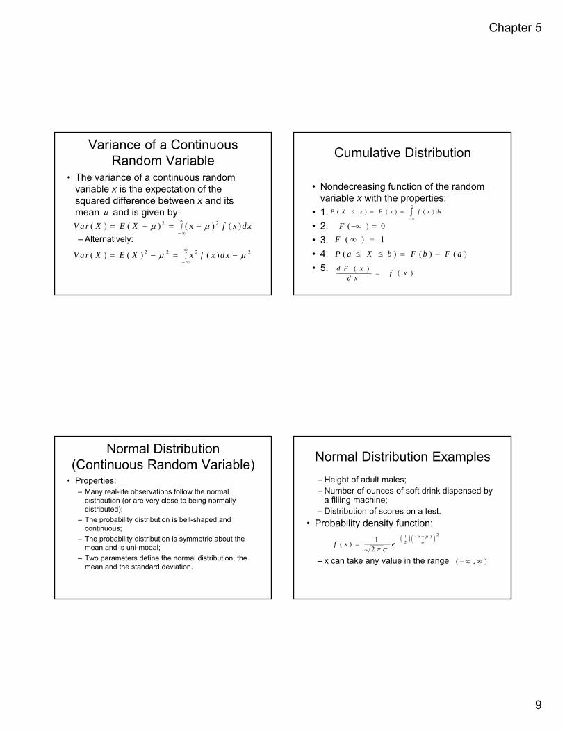
Variance of a Continuous Random Variable

• The variance of a continuous random variable x is the expectation of the squared difference between x and its mean and is given by:

– Alternatively:

V ar X E X x f x dx( ) ( ) ( ) ( )

2 2

V ar X E X x f x dx( ) ( ) ( )

2 2 2 2

Cumulative Distribution

• Nondecreasing function of the random variable x with the properties:

• 1.

• 2.

• 3.

• 4.

• 5.

x

dxxfxFxXP )()()(

0)( F

F ( ) 1

P a X b F b F a( ) ( ) ( )

d F xd x

f x( )

( )

Normal Distribution(Continuous Random Variable)

• Properties:– Many real-life observations follow the normal

distribution (or are very close to being normally distributed);

– The probability distribution is bell-shaped and continuous;

– The probability distribution is symmetric about the mean and is uni-modal;

– Two parameters define the normal distribution, the mean and the standard deviation.

Normal Distribution Examples

– Height of adult males;– Number of ounces of soft drink dispensed by

a filling machine;– Distribution of scores on a test.

• Probability density function:

– x can take any value in the range

f x ex

( )( )

1

2

1

2

2

( , )

Chapter 5

10

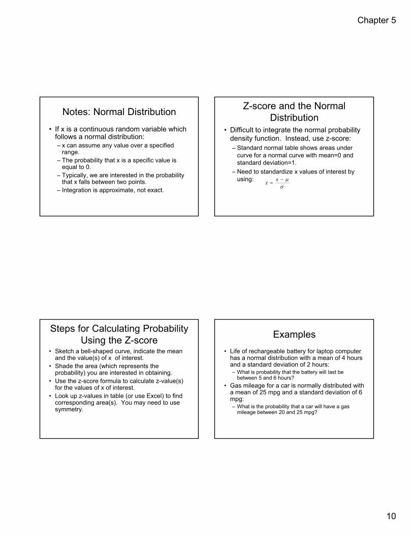
Notes: Normal Distribution

• If x is a continuous random variable which follows a normal distribution:– x can assume any value over a specified

range.– The probability that x is a specific value is

equal to 0.– Typically, we are interested in the probability

that x falls between two points.– Integration is approximate, not exact.

Z-score and the Normal Distribution

• Difficult to integrate the normal probability density function. Instead, use z-score:– Standard normal table shows areas under

curve for a normal curve with mean=0 and standard deviation=1.

– Need to standardize x values of interest by using:

zx

Steps for Calculating Probability Using the Z-score

• Sketch a bell-shaped curve, indicate the mean and the value(s) of x of interest.

• Shade the area (which represents the probability) you are interested in obtaining.

• Use the z-score formula to calculate z-value(s) for the values of x of interest.

• Look up z-values in table (or use Excel) to find corresponding area(s). You may need to use symmetry.

Examples

• Life of rechargeable battery for laptop computer has a normal distribution with a mean of 4 hours and a standard deviation of 2 hours:– What is probability that the battery will last be

between 5 and 6 hours?

• Gas mileage for a car is normally distributed with a mean of 25 mpg and a standard deviation of 6 mpg:– What is the probability that a car will have a gas

mileage between 20 and 25 mpg?

Chapter 5

11

Discrete Random Variables-Binomial Example

• The probability that a patient fails to recover from a particular operation in Fairfax Hospital is 0.1:– What is the probability that exactly two of the

next eight patients having this operation will not recover?

– What is the probability that at most one patient of the next eight patients having this operation will not recover?

Discrete Random Variables-Binomial Example 2

• Thirty percent of the defective brake calipers manufactured by Dana can be fixed by rework:– What is the probability that in a batch of six defective

calipers at least three can be fixed by rework?– What is the probability that none of them can be fixed

by rework?– What is the probability that all of them can be fixed by

rework?

Discrete Random Variables-Binomial Example 3

• Western Digital expects only 2% of its hard disks to malfunction during the warranty period. In a sample of ten disk drives:– What is the probability that none will malfunction

during the warranty period?

– What is the probability that exactly one will malfunction during the warranty period?

– What is the probability that at least two will malfunction during the warranty period?

Continuous Random Variables-Normal Example

• Let x be a random variable depicting human intelligence as measured by IQ tests. If x has a normal distribution with a mean of 100 and a standard deviation of 10, determine:– The probability of an IQ greater than 100;

– The probability of an IQ less than 85;

– The probability of an IQ of at least 110;

– The probability of an IQ between 85 and 125;

– The probability of an IQ between 110 and 200.

Chapter 5

12

Continuous Random Variables-Normal Example 2

• Suppose the outer diameter of a ball bearing produced by a stable manufacturing process follows a normal distribution with a mean of 3.5 cm and a standard deviation of 0.02 cm. If the diameter of this type of ball bearing must be no smaller than 3.47 cm and no larger than 3.53 cm to be usable, what percentage of bearings must be scrapped?

Continuous Random Variables-Normal Example 3

• A time and motion study was conducted at the Volvo-GM manufacturing plant in Dublin (VA) to determine the time it takes a worker to assemble the rear drive unit for a large truck. The data was found to be normally distributed with a mean of 75 seconds and a standard deviation of 6 seconds. In order for the assembly process to flow smoothly, this unit has to be assembled in 84 seconds or less. Approximately what proportion of the time will the assembly process flow smoothly?