Random Variables And Discrete Probability Distributions

Statistics for Management and Economics

Chapter 7

Objectives

Random Variables and Probability Distributions

Bivariate Distributions Binomial Distribution Poisson Distribution

Random Variables

A random variable is a function or rule that assigns a number to each outcome of an experiment.

Alternatively, the value of a random variable is a numerical event.

Instead of talking about the coin flipping event as

{heads, tails} think of it as “the number of heads when flipping a coin” so we have {1, 0}

Random Variables

Discrete one that takes on a

countable number of values

Values on the roll of dice: 2, 3, 4, …, 12

Integers

Continuous one whose values

are not discrete, not countable

Values resulting from the event time taken to walk to campus (anywhere from 5 to 30 minutes)

Real Numbers

Probability Distributions

A probability distribution is a table, formula, or graph that describes the values of a random variable and the probability associated with these values.

Since we’re describing a random variable (which can be discrete or continuous) we have two types of probability distributions: Discrete Probability Distribution, (this chapter)

Continuous Probability Distribution (Chapter 8)

Notation

An upper-case letter will represent the name of the random variable, usually X.

Its lower-case counterpart will represent the value of the random variable.

The probability that the random variable X will equal x is: P(X = x)

…or more simply P(x)

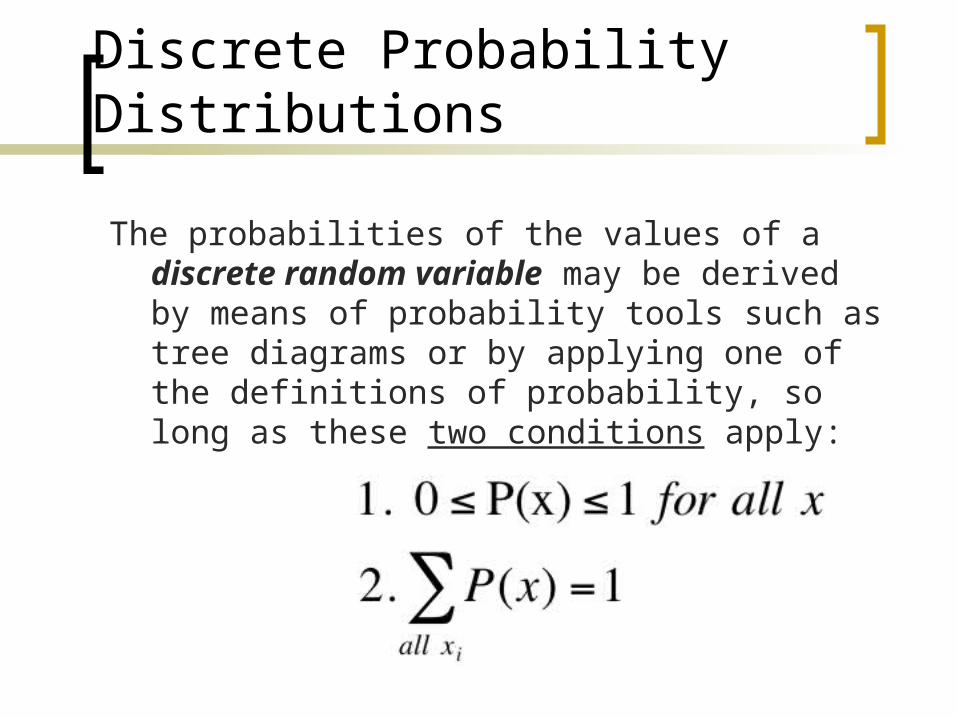
Discrete Probability Distributions

The probabilities of the values of a discrete random variable may be derived by means of probability tools such as tree diagrams or by applying one of the definitions of probability, so long as these two conditions apply:

Discrete DistributionsA survey of Amazon.com shoppers reveals the following probability distribution of he number of books purchased per hit:

# of books x P(x)

0 0 0.35

1 1 0.25

2 2 0.20

3 3 0.08

4 4 0.06

5 5 0.03

6 6 0.02

7 7 0.01

e.g. P(X=4) = P(4) = 0.06 = 6%

What is the probability that a shopper buys at least one book, but no more than 3 books?

P(1 ≤ X ≤ 3) = P(1) + P(2) + P(3) = 0.25 + 0.20 + 0.08

= 0.53

Developing a Probability Distribution

Probability calculation techniques can be used to develop probability distributions, for example, a new game in Vegas is developed where a fair coin is tossed three times.

What is the probability distribution of the number of heads if I play this game in Vegas?

Let H denote success, i.e. flipping a head P(H)=.50Thus HC is not flipping a head, and P(HC)=.50

Probability Distribution

The discrete probability distribution represents a population

Since we have populations, we can describe them by computing various parameters.

E.g. the population mean and population variance.

Population MeanUnivariate Discrete Probability Distribution

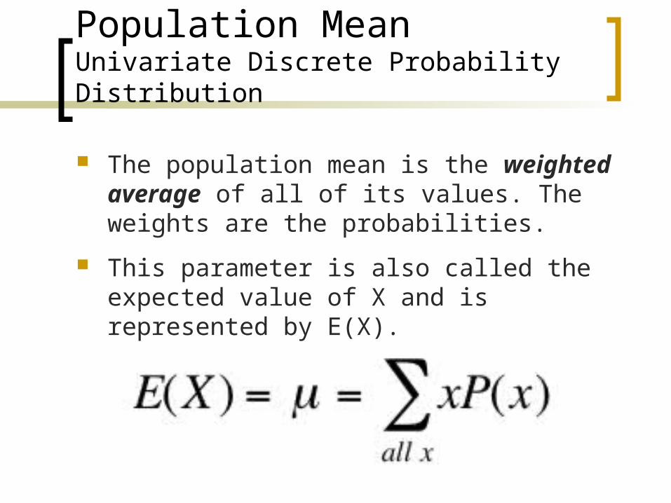
The population mean is the weighted average of all of its values. The weights are the probabilities.

This parameter is also called the expected value of X and is represented by E(X).

Population Variance Univariate Discrete Probability Distribution

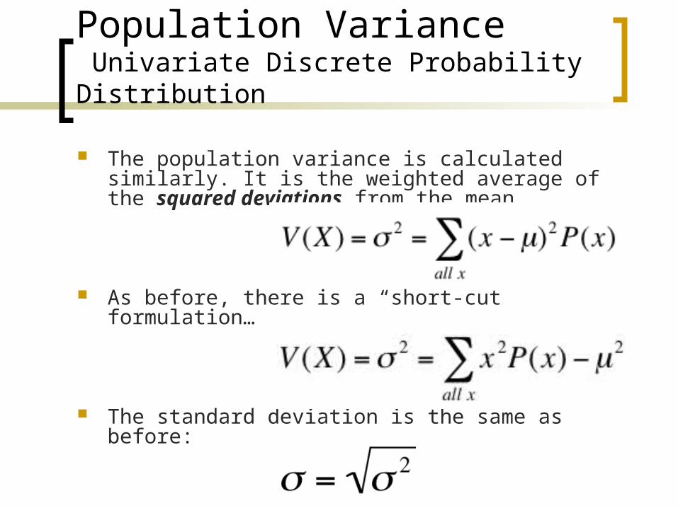
The population variance is calculated similarly. It is the weighted average of the squared deviations from the mean.

As before, there is a “short-cut” formulation…

The standard deviation is the same as before:

Population Mean, Variance, and Standard Deviation

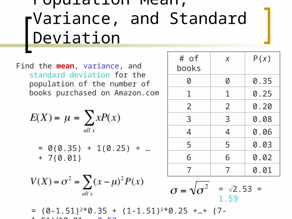
Find the mean, variance, and standard deviation for the population of the number of books purchased on Amazon.com

# of books

x P(x)

0 0 0.35

1 1 0.25

2 2 0.20

3 3 0.08

4 4 0.06

5 5 0.03

6 6 0.02

7 7 0.01

= 0(0.35) + 1(0.25) + … + 7(0.01)

= 1.51

= (0-1.51)2*0.35 + (1-1.51)2*0.25 +…+ (7-1.51)2*0.01 = 2.53

= 2.53 = 1.59

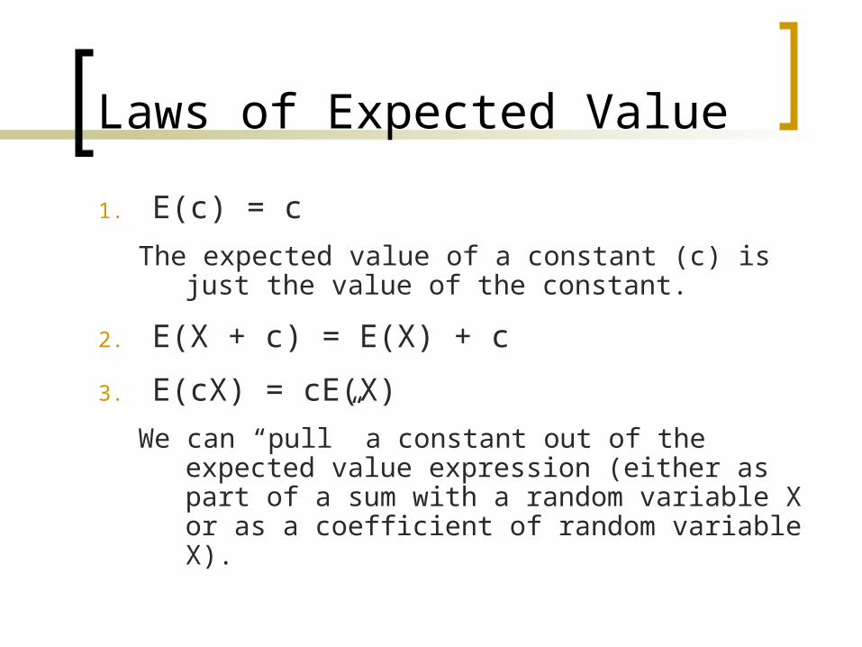
Laws of Expected Value

1. E(c) = c

The expected value of a constant (c) is just the value of the constant.

2. E(X + c) = E(X) + c

3. E(cX) = cE(X)

We can “pull” a constant out of the expected value expression (either as part of a sum with a random variable X or as a coefficient of random variable X).

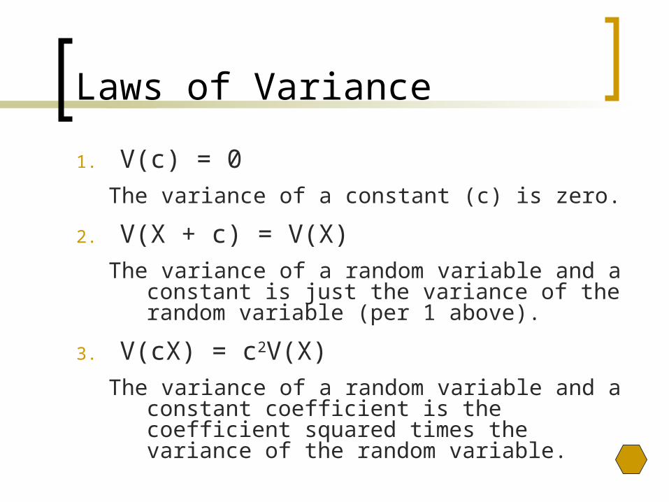
Laws of Variance

1. V(c) = 0The variance of a constant (c) is zero.

2. V(X + c) = V(X)The variance of a random variable and a constant is

just the variance of the random variable (per 1 above).

3. V(cX) = c2V(X) The variance of a random variable and a constant

coefficient is the coefficient squared times the variance of the random variable.

Bivariate Distributions

Up to now, we have looked at univariate distributions, i.e. probability distributions in one variable.

As you might guess, bivariate distributions are probabilities of combinations of two variables.

Bivariate probability distributions are also called joint probability. A joint probability distribution of X and Y is a table or formula that lists the joint probabilities for all pairs of values x and y, and is denoted P(x,y).

P(x,y) = P(X=x and Y=y)

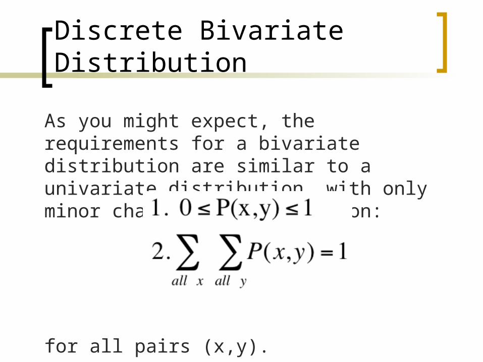
Discrete Bivariate Distribution

As you might expect, the requirements for a bivariate distribution are similar to a univariate distribution, with only minor changes to the notation:

for all pairs (x,y).

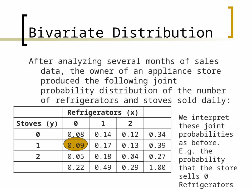
Bivariate Distribution

After analyzing several months of sales data, the owner of an appliance store produced the following joint probability distribution of the number of refrigerators and stoves sold daily:

Refrigerators (x)

Stoves (y) 0 1 2

0 0.08 0.14 0.12 0.34

1 0.09 0.17 0.13 0.39

2 0.05 0.18 0.04 0.27

0.22 0.49 0.29 1.00

We interpret these joint probabilities as before.E.g. the probability that the store sells 0 Refrigerators and 1 Stove in the day is P(0, 1) = 0.09

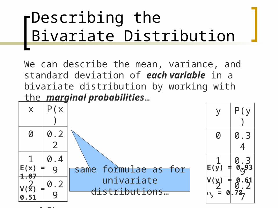
Describing the Bivariate Distribution

We can describe the mean, variance, and standard deviation of each variable in a bivariate distribution by working with the marginal probabilities…

x P(x)

0 0.22

1 0.49

2 0.29

y P(y)

0 0.34

1 0.39

2 0.27

E(x) = 1.07

V(x) = 0.51

x = 0.71

E(y) = 0.93

V(y) = 0.61

y = 0.78

same formulae as for univariate distributions…

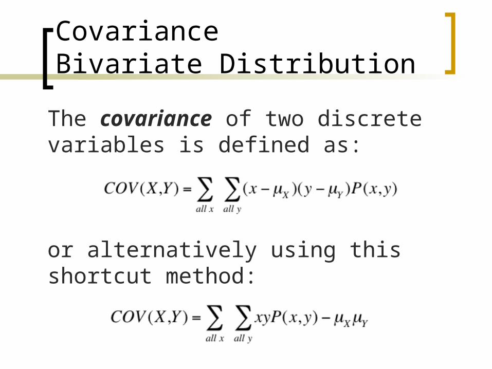
CovarianceBivariate Distribution

The covariance of two discrete variables is defined as:

or alternatively using this shortcut method:

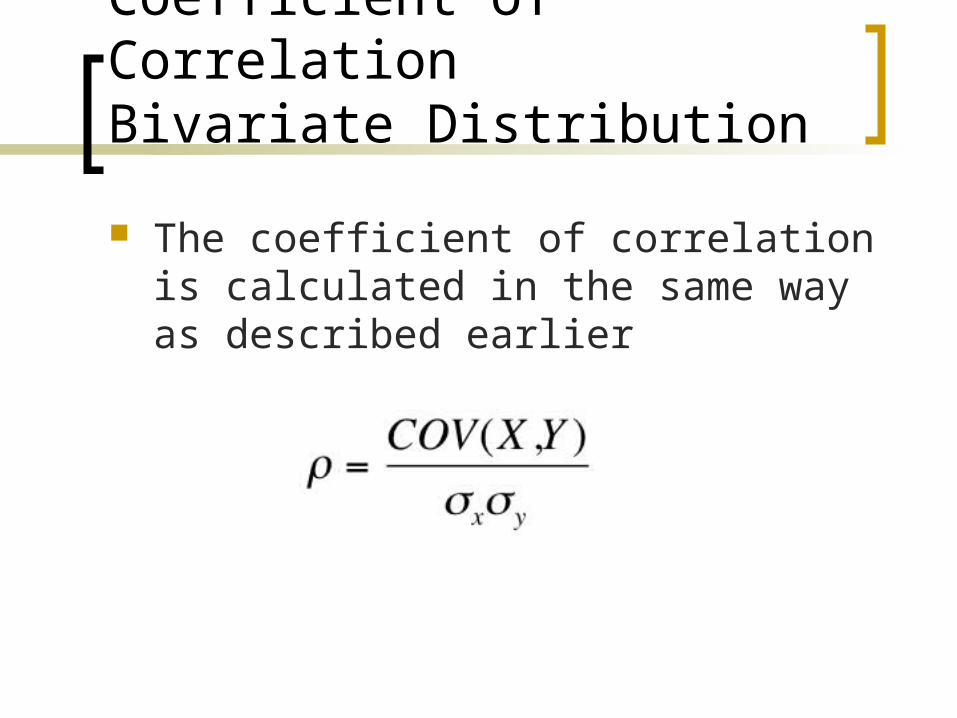
Coefficient of CorrelationBivariate Distribution

The coefficient of correlation is calculated in the same way as described earlier

Covariance and CorrelationBivariate Distribution

Compute the covariance and the coefficient of correlation between the numbers of refrigerators and stoves sold.

COV(X,Y) = (0 –1.07)(0 – 0.93)(0.08) + (1 – 1.07)(0 – 0.93)(0.14) + …… + (2 – 1.07)(2 – 0.93)(.04) = –0.045

= –0.045 ÷ [(.71)(.78)] = –0.081

There is a weak, negative relationship between the two variables.

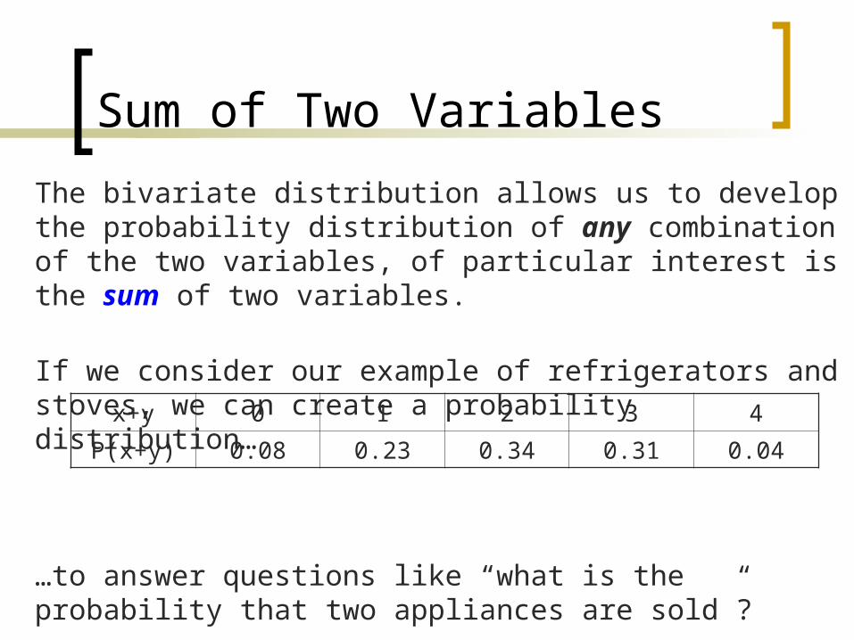
Sum of Two Variables

The bivariate distribution allows us to develop the probability distribution of any combination of the two variables, of particular interest is the sum of two variables.

If we consider our example of refrigerators and stoves, we can create a probability distribution…

…to answer questions like “what is the probability that two appliances are sold”?

P(X+Y=2) = P(0,2) + P(1,1) + P(2,0) = 0.05 + 0.17 + 0.12 = 0.34

x+y 0 1 2 3 4

P(x+y) 0.08 0.23 0.34 0.31 0.04

Laws: Bivariate Distribution

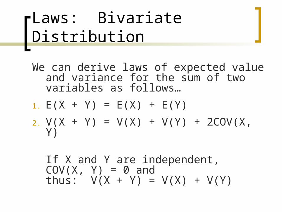
We can derive laws of expected value and variance for the sum of two variables as follows…

1. E(X + Y) = E(X) + E(Y)

2. V(X + Y) = V(X) + V(Y) + 2COV(X, Y)

If X and Y are independent, COV(X, Y) = 0 and thus: V(X + Y) = V(X) + V(Y)

Binomial Distribution

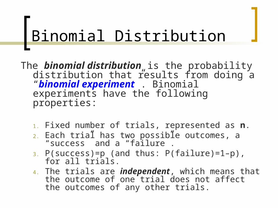
The binomial distribution is the probability distribution that results from doing a “binomial experiment”. Binomial experiments have the following properties:

1. Fixed number of trials, represented as n.2. Each trial has two possible outcomes, a “success”

and a “failure”.3. P(success)=p (and thus: P(failure)=1–p), for all

trials.4. The trials are independent, which means that the

outcome of one trial does not affect the outcomes of any other trials.

“Success” and “Failure”

…are just labels for a binomial experiment, there is no value judgment implied.

For an experiment to b binomial, it simply must have two possible outcomes: something happens or something doesn’t happen.

For example a coin flip will result in either heads or tails. If we define “heads” as success then necessarily “tails” is considered a failure (inasmuch as we attempting to have the coin lands heads up).

Other binomial experiment notions: An election candidate wins or loses An employee is male or female

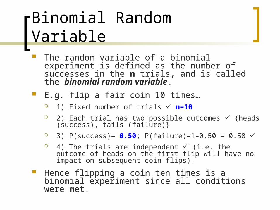
Binomial Random Variable The random variable of a binomial experiment is

defined as the number of successes in the n trials, and is called the binomial random variable.

E.g. flip a fair coin 10 times… 1) Fixed number of trials n=10 2) Each trial has two possible outcomes {heads

(success), tails (failure)} 3) P(success)= 0.50; P(failure)=1–0.50 = 0.50 4) The trials are independent (i.e. the outcome of heads

on the first flip will have no impact on subsequent coin flips).

Hence flipping a coin ten times is a binomial experiment since all conditions were met.

Binomial Random Variable

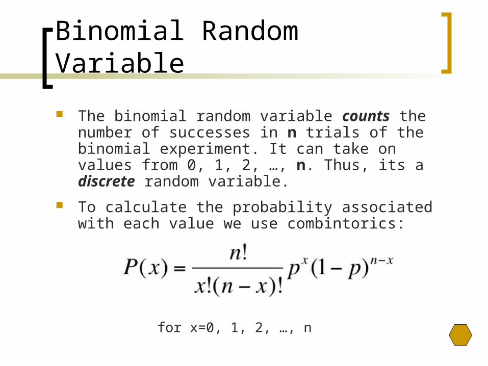
The binomial random variable counts the number of successes in n trials of the binomial experiment. It can take on values from 0, 1, 2, …, n. Thus, its a discrete random variable.

To calculate the probability associated with each value we use combintorics:

for x=0, 1, 2, …, n

Rule of Combinations

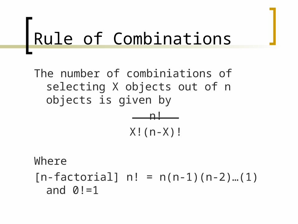
The number of combiniations of selecting X objects out of n objects is given by

n!

X!(n-X)!

Where

[n-factorial] n! = n(n-1)(n-2)…(1) and 0!=1

Rule of Combinations

Often denoted by the symbol nX

Thus… with n=4 and x=3…

n! 4! 4x3x2x1 4

X!(n-X)! 3!(4-3)! (3x2x1)(1) == =

So, there are 4 such sequences, each with the same probability of 0.0009. The probability of obtaining exactly three tagged order forms is equal to (number of possible sequences) X (probability of a particular sequence)

Binomial Distribution

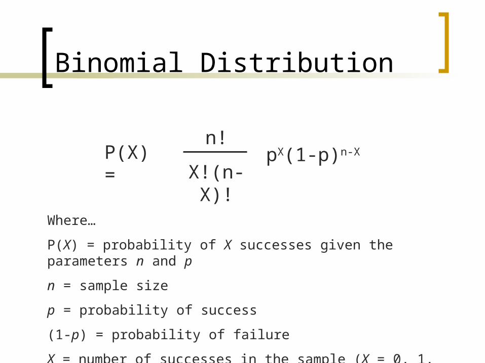
P(X) =n!

X!(n-X)!pX(1-p)n-X

Where…

P(X) = probability of X successes given the parameters n and p

n = sample size

p = probability of success

(1-p) = probability of failure

X = number of successes in the sample (X = 0, 1, 2, …, n)

E.C.K. Pharmaceutical Company

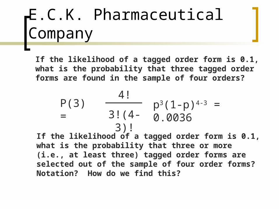
If the likelihood of a tagged order form is 0.1, what is the probability that three tagged order forms are found in the sample of four orders?

P(3) =4!

3!(4-3)!p3(1-p)4-3 = 0.0036

If the likelihood of a tagged order form is 0.1, what is the probability that three or more (i.e., at least three) tagged order forms are selected out of the sample of four order forms? Notation? How do we find this?

Cumulative Probability

Thus far, we have been using the binomial probability distribution to find probabilities for individual values of x. To answer the question:

“Find the probability that the order is tagged”

requires a cumulative probability, that is, P(X ≤ x)

What is the probability that we find fewer than three tagged order forms in the sample of four orders?

Thus, we want to know what is: P(X ≤ 3) to answer

Cumulative ProbabilityP(X ≤ 3) = P(X=0) + P(X=1) + P(X=2) + P(X=3)

Use the binomial probability to find…

P(2) =4!

2!(4-2)!p2(1-p)4-2 = 0.0486

P(0) =4!

0!(4-0)!p0(1-p)4-0 = 0.6561

P(1) =4!

1!(4-1)!p1(1-p)4-1 = 0.2916

P(X ≤ 3) = 0.9963

Is there another way to get this?

Binomial Table

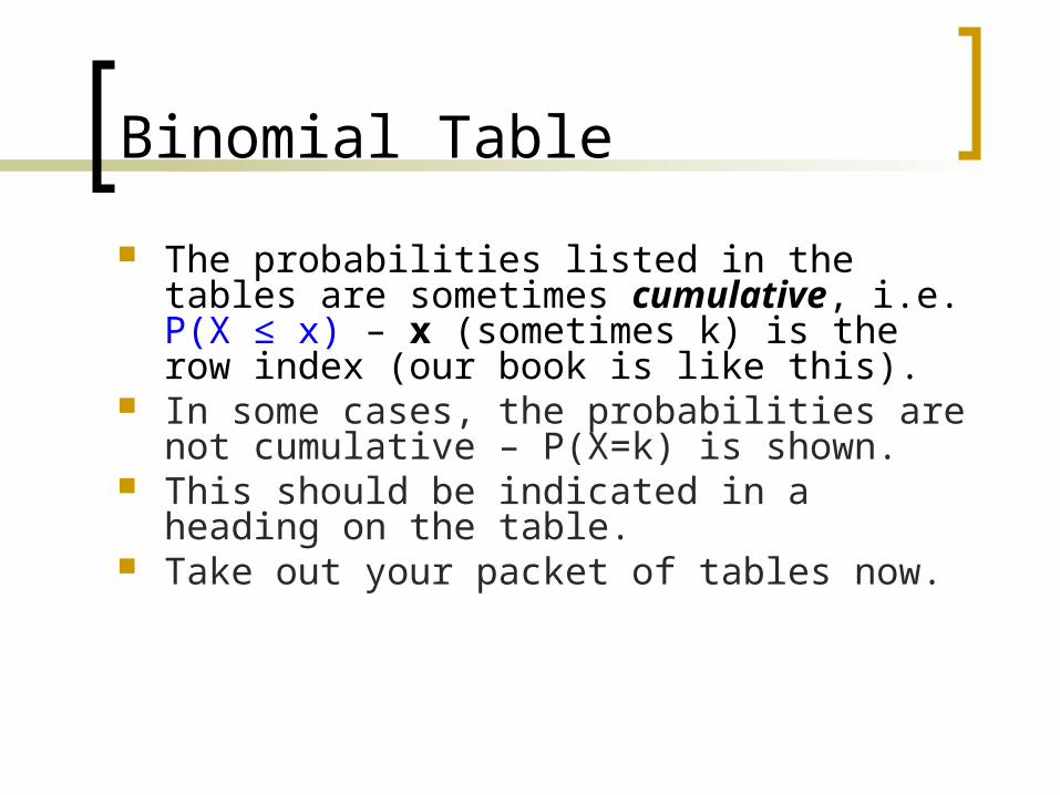
The probabilities listed in the tables are sometimes cumulative, i.e. P(X ≤ x) – x (sometimes k) is the row index (our book is like this).

In some cases, the probabilities are not cumulative – P(X=k) is shown.

This should be indicated in a heading on the table.

Take out your packet of tables now.

Binomial TableFor a binomial table that gives cumulative probabilities

for P(X ≤ k)…

P(X = k) = P(X ≤ k) – P(X ≤ [k–1])

Likewise, for probabilities given as P(X ≥ k), we have:P(X ≥ k) = 1 – P(X ≤ [k–1])

However, if the table does not give cumulative probabilities, as we saw in the example, in order to

find P(X ≤ k) you have to add the k-1, etc probabilities.

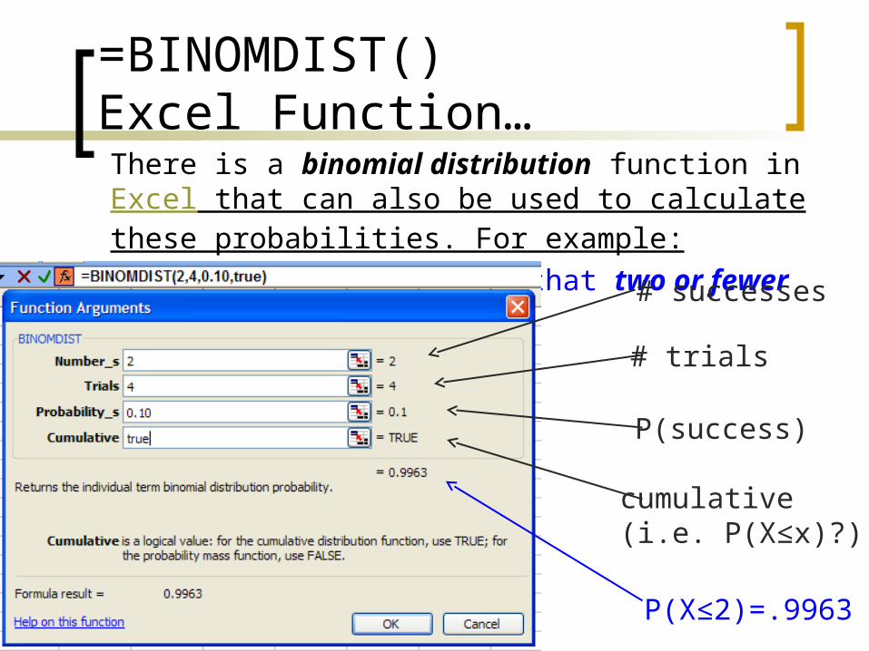
=BINOMDIST() Excel Function…There is a binomial distribution function in Excel that can also be used to calculate these probabilities. For example:

What is the probability that two or fewer orders are tagged?

# successes

# trials

P(success)

cumulative(i.e. P(X≤x)?)

P(X≤2)=.9963

Binomial DistributionAs you might expect, statisticians have developed general formulas for the mean, variance, and standard deviation of a binomial random variable. They are:

Poisson Distribution

Named for Simeon Poisson, the Poisson distribution is a discrete probability distribution and refers to the number of events (a.k.a. successes) within a specific time period or region of space. For example:o The number of cars arriving at a service station in 1 hour.

(The interval of time is 1 hour.) o The number of flaws in a bolt of cloth. (The specific

region is a bolt of cloth.)o The number of accidents in 1 day on a particular stretch

of highway. (The interval is defined by both time, 1 day, and space, the particular stretch of highway.)

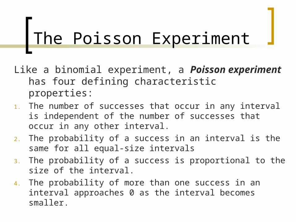
The Poisson Experiment

Like a binomial experiment, a Poisson experiment has four defining characteristic properties:

1. The number of successes that occur in any interval is independent of the number of successes that occur in any other interval.

2. The probability of a success in an interval is the same for all equal-size intervals

3. The probability of a success is proportional to the size of the interval.

4. The probability of more than one success in an interval approaches 0 as the interval becomes smaller.

Poisson Distribution

The Poisson random variable is the number of successes that occur in a period of time or an interval of space in a Poisson experiment.

E.g. On average, 96 trucks arrive at a border crossing every hour.

E.g. The number of typographic errors in a new textbook edition averages 1.5 per 100 pages.

successes

time period

successes (?!) interval

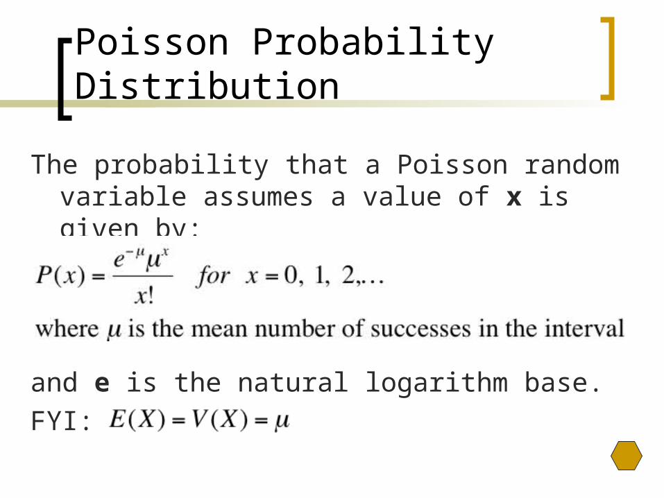
Poisson Probability Distribution

The probability that a Poisson random variable assumes a value of x is given by:

and e is the natural logarithm base.

FYI:

=Poisson Excel Function