random trees - département de mathématiques d'orsay

Random trees

Jean-François Le Gall

Université Paris-Sud Orsay and Institut universitaire de France

IMS Annual Meeting, Göteborg, August 2010

Jean-François Le Gall (Université Paris-Sud) Random trees Göteborg 1 / 40

Outline

Trees are mathematical objects that play an important role in severalareas of mathematics and other sciences:

Combinatorics, graph theory (trees are simple examples ofgraphs, and can also be used to encode more complicatedgraphs)

Probability theory (trees as tools to study Galton-Watsonbranching processes and other random processes describing theevolution of populations)

Mathematical biology (population genetics, connections withcoalescent processes)

Theoretical computer science (trees are important cases of datastructures, giving ways of storing and organizing data in acomputer so that they can be used efficiently)


Our goal

To understand the properties of “typical” large trees.A typical tree will be generated randomly :

Combinatorial tree: By choosing this tree uniformly at random in acertain class of trees (plane trees, Cayley trees, binary trees, etc.)of a given size.

Galton-Watson tree: By choosing randomly the number of“children” of the root, then recursively the number of children ofeach child of the root, and so on.

There are many other ways of generating random trees, for instance,

Binary search trees (used in computer science)

Preferential attachment models (Barabási-Alberts) used to modelthe World Wide Web.


What results are we aiming at?

Limiting distributions for certain characteristics of the tree, when itssize tends to infinity:

Height, width of the tree

Profile of distances in the tree (how many vertices at eachgeneration of the tree)

More refined genealogical quantities.

Often information about these asymptotic distributions can be derivedby studying scaling limits:

⇒ Find a continuous model (continuous random tree) such that the(suitably rescaled) discrete random tree with a large size is close tothis continuous model.

Strong analogy with the classical invariance theorems relating randomwalks to Brownian motion.


Examples of discrete trees - Plane trees

v

v

v

v v v

v

v

v

∅

v21

11 12

123122121

111

1231

A plane treeτ = {∅,1,2,11,12, . . .}

A plane tree (or rooted ordered tree) is afinite subset τ of

∞⋃

n=0

Nn

where N = {1,2,3, . . .} and N0 = {∅},

such that:

∅ ∈ τ .

If u = u1 . . . un ∈ τ\{∅} thenu1 . . . un−1 ∈ τ .

For every u = u1 . . . un ∈ τ , thereexists ku(τ) ≥ 0 such that

u1 . . . unj ∈ τ iff 1 ≤ j ≤ ku(τ).

(ku(τ) = number of children of u in τ )


Other discrete trees

Unordered rooted trees

t

t

tt

t

t

=

t

t

t

t

t

t

Two different plane treesthe same unordered rooted tree

Cayley trees

��

�

��

��

��

@@

@�

��

t

t

t

t

t

t

1 2

3

45

6A Cayley tree on 6 vertices(= connected graph on {1,2, . . . ,6} withno loop)

Binary trees : plane trees with 0 or 2 children for each vertex


1. Scaling limits of contour functions

µ = offspring distribution (probability distribution on {0,1,2, . . .})Assume µ is critical :

∑∞k=0 k µ(k) = 1 and µ(1) < 1.

v

v

v

v v v

v

v

v

∅

v21

11 12

123122121

111

1231 A µ-Galton-Watson tree θ is a random plane treesuch that:

Each vertex has k children with probabilityµ(k).

The numbers of children of the differentvertices are independent.

Formally, for each fixed τ ∈ T := {plane trees},

P(θ = τ) =∏

u∈τ

µ(ku(τ)).


Important special cases

Geometric distribution

µ(k) = 2−k−1

Then, if |τ | = number of edges of τ ,

P(θ = τ) = 2−2|τ |−1.

Consequence: The conditional distribution of θ given |θ| = p isuniform over {plane trees with p edges}.

Poisson distribution

µ(k) =e−1

k!

The conditional distribution of θ given |θ| = p is uniform over{Cayley trees on p + 1 vertices}.(Needs to view a plane tree as a Cayley tree by “forgetting” theorder and randomly assigning labels 1,2, . . . to vertices)


Coding trees by contour functions

AA

AA

��

AA

AA

��

AA

AA

��

AAK

AAK AAU6

AAK AAU ��

?��

AAU ��

∅

1 2

11 12 13

121 122

A plane tree τ withp edges (or p + 1 vertices)

-

6

��DDDDD��DDDDD��DDDDDDDDDD��DDDDDDDDDD��DDDDD

1

2

1 2 3 2p

Cτ (s)

s

and its contour function(Cτ (s),0 ≤ s ≤ 2p)

A plane tree can be coded by its contour function (or Dyck path incombinatorics)


Aldous’ theorem (finite variance case)

Theorem (Aldous)Let θp be a µ-Galton-Watson tree conditioned to have p edges. Then

( 1√

2pCθp(2pt)

)

0≤t≤1

(d)−→p→∞

(

√2σ

et

)

0≤t≤1

where σ2 = var(µ) and (et)0≤t≤1 is a normalized Brownian excursion.

6

6K

O W

�

?�

�

?t

et

11

1/√

2p

1/2p

−→p → ∞

s

s s s

ss

s s

s s s


The normalized Brownian excursion

To construct a normalizedBrownian excursion (et)0≤t≤1:

Consider a Brownian motion(Bt)t≥0 with B0 = ε.

Condition on the event

inf{t ≥ 0 : Bt = 0} = 1

Let ε→ 0. t

Bt

ε

1More intrinsic approaches via Itô’s excursion theory.


An application of Aldous’ theorem

Let h(θp) = height of θp (= maximum of contour function). Then

P[h(θp) ≥ x√

p] −→p→∞

P

[

max0≤t≤1

et ≥σx2

]

The RHS is known in the form of a series (Chung 1976)

P

[

max0≤t≤1

et ≥ x]

= 2∞

∑

k=1

(4k2x2 − 1) exp(−2k2x2).

Special case µ(k) = 2−k−1 : asymptotic proportion of those trees withp edges whose height is greater than x

√p.

cf results from theoretical computer science, Flajolet-Odlyzko (1982)

General idea:

The limit theorem for the contour gives the “asymptotic shape” of thetree, from which one can derive – or guess – many asymptotics forspecific functionals of the tree.


2. The CRT and Gromov-Hausdorff convergence

Aldous’ theorem suggests that

There exists a continuous random tree which is the universal limitof (rescaled) Galton-Watson trees conditioned to have n edges,

and whose “contour function” is the Brownian excursion.

In other words we want to make sense of the convergence

σ

2√

pθp

(d)−→p→∞

Te

For this, we need:

to say what kind of an object the limit is (a random real tree)

to explain how a real tree can be coded by a function (here by e)

to say in which sense the convergence holds (in theGromov-Hausdorff sense)


The Gromov-Hausdorff distanceThe Hausdorff distance. K1, K2 compact subsets of a metric space

dHaus(K1,K2) = inf{ε > 0 : K1 ⊂ Uε(K2) and K2 ⊂ Uε(K1)}(Uε(K1) is the ε-enlargement of K1)

Definition (Gromov-Hausdorff distance)If (E1,d1) and (E2,d2) are two compact metric spaces,

dGH(E1,E2) = inf{dHaus(ψ1(E1), ψ2(E2))}the infimum is over all isometric embeddings ψ1 : E1 → E andψ2 : E2 → E of E1 and E2 into the same metric space E .

ψ2

E2E1

ψ1


Gromov-Hausdorff convergence of rescaled trees

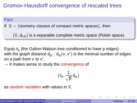
FactIf K = {isometry classes of compact metric spaces}, then

(K,dGH) is a separable complete metric space (Polish space)

Equip θp (the Galton-Watson tree conditioned to have p edges)with the graph distance dgr : dgr(v , v ′) is the minimal number of edgeson a path from v to v ′.→ It makes sense to study the convergence of

(θp,1√p

dgr)

as random variables with values in K.


The notion of a real tree

DefinitionA real tree is a (compact) metric space T suchthat:

any two points a,b ∈ T are joined by aunique arc

this arc is isometric to a line segment

It is a rooted real tree if there is a distinguishedpoint ρ, called the root.

ab

ρ

Remark. A real tree can have

infinitely many branching points

(uncountably) infinitely many leaves

Fact. The coding of plane trees by contour functions can be extendedto real trees.


The real tree coded by a function g

g : [0,1] −→ [0,∞)continuous,g(0) = g(1) = 0

mg(s,t)

g(s)

g(t)

s t ′t 1

mg(s, t) = mg(t , s) = mins≤r≤t g(r)

dg(s, t) = g(s) + g(t) − 2mg(s, t) t ∼ t ′ iff dg(t , t ′) = 0

Proposition (Duquesne-LG)Tg := [0,1]/∼ equipped with dg is a real tree, called the tree coded byg. It is rooted at ρ = 0.

Remark. Tg inherits a “lexicographical order” from the coding.Jean-François Le Gall (Université Paris-Sud) Random trees Göteborg 17 / 40

Aldous’ theorem revisitedTheoremIf θp is a µ-Galton-Watson tree conditioned to have p edges,

(θp,σ

2√

pdgr)

(d)−→p→∞

(Te,de)

in the Gromov-Hausdorff sense.

The limit (Te,de) is the (random) real tree coded by a Brownianexcursion e. It is called the CRT (Continuum Random Tree).

1t

et

ρ

tree Te

�IyzIw�o


Application to combinatorial trees

By choosing appropriately the offspring distribution, one obtains thatthe CRT is the scaling limit of

plane trees

(ordered) binary trees

Cayley trees

with size p, with the same rescaling 1/√

p (but different constants).

It is also true that the CRT is the scaling limit of

unordered binary trees

but this is much harder to prove (no connection with Galton-Watsontrees), see Marckert-Miermont 2009.


The stick-breaking construction of the CRT (Aldous)

Consider a sequence X1,X2, . . . of positive random variables such that,for every n ≥ 1, the vector (X1,X2, . . . ,Xn) has density

an x1(x1 + x2) · · · (x1 + · · · + xn) exp(−2(x1 + · · · + xn)2)

Then “break” the positive half-line into segments of lengths X1,X2, . . .and paste them together to form a tree :

X1

The first branch has length X1

The second branch has length X2 and isattached at a point uniform over the first branch

The third branch has length X3 and is attachedat a point uniform over the union of the first twobranches

And so on




an x1(x1 + x2) · · · (x1 + · · · + xn) exp(−2(x1 + · · · + xn)2)


X1X2




And so on




an x1(x1 + x2) · · · (x1 + · · · + xn) exp(−2(x1 + · · · + xn)2)


X1

X3

X2




And so on




an x1(x1 + x2) · · · (x1 + · · · + xn) exp(−2(x1 + · · · + xn)2)


X1

X3

X2

X4




And so on


The stick-breaking construction of the CRT (Aldous)Consider a sequence X1,X2, . . . of positive random variables such that,for every n ≥ 1, the vector (X1,X2, . . . ,Xn) has density

an x1(x1 + x2) · · · (x1 + · · · + xn) exp(−2(x1 + · · · + xn)2)





And so on

Finally take the completion to get the CRT


3. The connection with random walk

t

t t

t t t t

t

t

Tree τ

-

6

t

n

Sn

1 2

1

2

3

3 |τ |+1

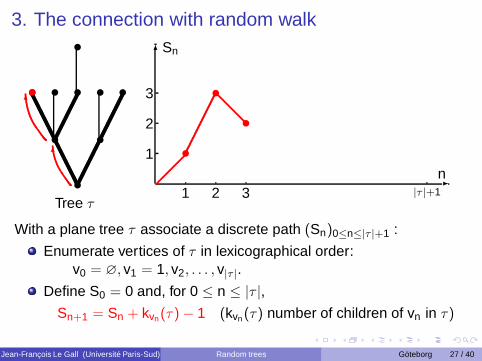
With a plane tree τ associate a discrete path (Sn)0≤n≤|τ |+1 :

Enumerate vertices of τ in lexicographical order:v0 = ∅, v1 = 1, v2, . . . , v|τ |.

Define S0 = 0 and, for 0 ≤ n ≤ |τ |,Sn+1 = Sn + kvn(τ) − 1 (kvn(τ) number of children of vn in τ)



t

t

t

t

t t t t

t

6

t

Tree τ

-

6

t

t

n

Sn

1 2

1

2

3

3 |τ |+1






t

t

t

t

t t t t

t

6

6

t

Tree τ

-

6

t

t

t

n

Sn

1 2

1

2

3

3 |τ |+1






t

t

t

t

t t t

t

6

6

jt

Tree τ

-

6

t

t

t

t

n

Sn

1 2

1

2

3

3 |τ |+1






t

t

t

t

t t t t

t

6

6

j q

�

N

�q

Tree τ

-

6

t

t

t

t t

t

t

t

t

n

Sn

1 2

1

2

3

3 |τ |+1





The random walk associated with a tree

t

t

t

t

t t t t

t

6

6

j q

�

N

�q

Tree τ

-

6

t

t

t

t t

t

t

t

t

n

Sn

1 2

1

2

3

3 |τ |+1

Recall Sn+1 = Sn + kvn(τ) − 1 (kvn(τ) number of children of vn in τ)

FactIf τ = θ is a Galton-Watson tree with offspring distribution µ,(Sn)0≤n≤|τ |+1 is a random walk with jump distribution ν(k) = µ(k + 1),k = −1,0,1, . . . stopped at its first hitting time of −1.


Sketch of proofRecall Sn+1 = Sn + kvn(τ) − 1 (kvn(τ) number of children of vn in τ)

For a µ-Galton-Watson tree, the r.v. kvn(τ) − 1 are i.i.d. withdistribution ν(k) = µ(k + 1).

S|τ |+1 =∑

0≤n≤|τ |

(kvn(τ) − 1) =(

∑

0≤n≤|τ |

kvn(τ))

− |τ | − 1

= |τ | − |τ | − 1

= −1

For 1 ≤ m ≤ |τ |,

Sm =∑

0≤n≤m−1

(kvn(τ) − 1) =∑

0≤n≤m−1

kvn(τ) − m ≥ 0

because among all individuals counted in∑

0≤n≤m−1 kvn(τ), thevertices v1, v2, . . . , vm all appear.


An application to the total progeny

CorollaryThe total progeny of a µ-Galton-Watson tree has the same distributionas the first hitting time of −1 by a random walk with jump distributionν(k) = µ(k + 1).

Proof. Just use the identity |τ | + 1 = min{n ≥ 0 : Sn = −1}.

Cf Harris (1952), Dwass (1970), etc.


Proof of Aldous’ theorem INeeds the “height function” associated with a plane tree τ .

t

t

t

t

t t t t

t

6

6

j q

�

N

�q

Tree τ

-

6

n1 2

1

2

3

3

t

t t t

t

t

t t

|τ |

Hn

If τ = {v0, v1, . . . , v|τ |} (in lexicogr. order), Hn = |vn| (generation of vn).

Lemma (Key formula)If S is the random walk associated with τ , then for 0 ≤ n ≤ |τ |,

Hn = #{j ∈ {0,1, . . . ,n − 1} : Sj = minj≤i≤n

Si}.


The key formula: Hn = #{j ∈ {0,1, . . . ,n − 1} : Sj = minj≤i≤n Si}.

t

t

t

t

t t t t

tv5

6

6

j q

�

N

�q

-

6

n1 2

1

2

3

3

t

t t t

t

t

t t

|τ |n=5

Hn

For n = 5, 3 values of j ≤ n − 1 such that Sj = minj≤i≤n Si .

-

6

t

t

t

t t

t

t

t

t

n

Sn

1 2

1

2

3

3 |τ |+1

t t

t

n=5


Proof of Aldous’ theorem IIFrom the key formula,

Hn = #{j ∈ {0,1, . . . ,n − 1} : Sj = minj≤i≤n

Si}

one can deduce that, for a Galton-Watson tree τ conditioned to have|τ | = p,

Hn ≈ 2σ2 S(p)

n ,0 ≤ n ≤ p

where S(p) is distributed as S conditioned to hit −1 at time p + 1.By a conditional version of Donsker’s theorem,

( 1σ√

pS(p)

[pt]

)

0≤t≤1

(d)−→p→∞

(et)0≤t≤1.

Finally, argue that

Cθp(2pt) ≈ H[pt] ≈2σ2 S(p)

[pt].


4. More general offspring distributions

What happens if we remove the assumption that µ has finite variance ?

−→ Get more general continuous random trees

−→ Coded by “excursions” which are no longer Brownian

Assumption (Aα)The offspring distribution µ has mean 1 and is such that

µ(k) ∼k→∞

c k−1−α

for some α ∈ (1,2) and c > 0

In particular, µ is in the domain of attraction of a stable distribution withindex α.


A “stable” version of Aldous’ theorem

Theorem (Duquesne)

Under Assumption (Aα), let (Cp(n))0≤n≤2p be the contour function of aµ-Galton-Watson tree conditioned to have p edges. Then,

( 1p1−1/α

Cp(2pt))

0≤t≤1

(d)−→p→∞

(c eαt )0≤t≤1,

where eα is defined in terms of the normalized excursion Xα of astable process with index α and nonnegative jumps:

eαt = “measure”{s ∈ [0, t] : Xα

s = infs≤r≤t

Xαr }.

The last formula is to be understood in a “local time” sense:

eαt = lim

ε→0

1ε

∫ t

0ds 1{Xα

s < infs≤r≤t

Xαr + ε}.


Why the process eα ?As in the proof of Aldous’ theorem,

Cp2pt ≈ Hp

[pt]

where (key formula), for 0 ≤ n ≤ p,

Hpn = #{j ∈ {0,1, . . . ,n − 1} : Sp

j = minj≤i≤n

Spi } (1)

and Sp is distributed as a random walk with jump distributionν(k) = µ(k + 1), conditioned to hit −1 at time p + 1.By the assumption on µ,

(

n−1/α Sp[pt]

)

0≤t≤1

(d)−→p→∞

(

c Xαt

)

0≤t≤1.

Then pass to the limit in (1): The (suitable rescaled) RHS of (1)converges to

“measure”{s ∈ [0, t] : Xαs = inf

s≤r≤tXα

r }.


Convergence of treesCorollaryUnder Assumption (Aα), let θp be a µ-Galton-Watson tree conditionedto have p edges. Then, if dgr denotes the graph distance on θp,

(θp,1

p1−1/αdgr)

(d)−→p→∞

(Teα , c deα)

in the Gromov-Hausdorff sense.Here (Teα ,deα) is the tree coded by the “stable excursion” eα.

The random tree (Teα ,deα) is called the stable tree with index α.

Can investigate probabilistic and fractal properties of stable trees indetail (Duquesne, LG). For instance,

dim Teα =α

α− 1

and level sets of Teα have dimension 1α−1 .


Extensions

For any “ branching mechanism function” ψ of the form

ψ(u) = a u + b u2 +

∫

(0,∞)π(dr) (e−ru − 1 + ru)

where a,b ≥ 0 and∫

(0,∞) π(dr) (r ∧ r2) <∞,

one can define a ψ-Lévy tree, which is a continuous random tree:

if ψ(u) = u2, this is Aldous’ CRT

if ψ(u) = uα, this is the stable tree with index α.

Lévy trees are

closely related to the Lévy process with Laplace exponent ψ

the possible scaling limits of (sub)critical Galton-Watson trees

characterized by a branching property analogous to the discretecase (Weill).


random trees - département de mathématiques d'orsay

Documents