random graphs - washington state university€¦ · graph invariants in random graphs • the...

Random Graphs Assefaw Gebremedhin

CptS 591: Elements of Network Science

1

Assefaw Gebremedhin, CptS 591: Elements of Network Science, http://scads.eecs.wsu.edu

Outline

• Random graph as a concept

• Random variables and Expectation

• Graph invariants in random graphs

• Phase transition

• Random graphs vs real-world networks (subject of next lecture)

2


Motivation (from graph theoretic perspective)

• Given a graph G, •  the minimum length of a cycle contained in G is the girth g(G) of G •  the maximum length of a cycle in G is its circumference •  the smallest number of colors required to color G is the chromatic number

x(G) of G • Example:

3

2

3

3 1 2

1 •  g(G) = 3 •  circumference(G) = 6 •  x(G) = 3 (in general NP-hard to compute)


Motivation (cont’d): Paraphrased Erdos theorem

•  There exist graphs whose 1.  girth is arbitrarily large, and 2.  chromatic number is arbitrarily large

•  These requirements work against each other: A graph with a large girth is tree-like (acyclic) and hence is expected to have small

chromatic number

•  è a constructive proof for Erdos theorem is difficult (if not impossible) to come by

•  Instead, Erdos used Random Graphs and the “Probabilistic Method” to prove such existence theorems

4


What is a random graph? •  Let V be a fixed set of n elements, say V ={1,2,…,n}. Let Ĝ be the set of all possible graphs on V.

(Note: there are 2N possible graphs N = (n:2), where (n:k) denotes n choose k)

•  We would like to turn Ĝ into a probability space and be able to answer such questions as •  What is the probability that a graph G in Ĝ has a certain property? •  What is the expected value of a given invariant on G?

•  Consider the following random process of generating G. •  Let [V]2 denote the set of all pairs of elements drawn from V

(There are (n:2) possible pairs) •  For each e in [V]2 decide using a random expt whether or not e shall be an edge of G •  Perform the expts independently, each time accepting e to be an edge with a fixed probability p, 0<=p<= 1

•  Now let G0 be some fixed graph on V with m edges. •  Then,

P[G=G0] = pm q(N-m) , where q = 1-p and N= (n:2)

5


What is random graph (cont’d) • One can continue in this way to determine probabilities of all possible

elementary events (all m) è the probability measure of the desired space Ĝ is determined • One can formally show (as in Diestel) that a probability measure on Ĝ

where all individual edges occur independently with probability p exists.

• With these two assumptions, we can now calculate probabilities in the

space Ĝ = Ĝ(n,p).

6


Examples • Let G in Ĝ, and H be a fixed graph on a subset U of V. Let the number

of vertices in H be k, and the number of edges be l. • Q1: What is P[H is a subgraph of G]? • Soln 1: Each edge of H occurs independently with a probability of p.

Hence the required probability is pl.

• Q2: What is P[H is an induced subgraph of G]? • Soln2: This time, in addition to that in Q1, the r = (k:2) – l edges

missing from H are required to be missing from G too, independently with probability q = 1-p.

Hence the required probability is plqr

7


More interesting examples

•  First we define a few notions •  Independent Set: a set of pairwise non-adjacent vertices •  Clique: a set of pairwise adjacent vertices •  The size of the largest IS in a graph G is its independence number α(G) •  The size of the largest clique in a graph is its clique number ω(G)

•  Lemma 1: For all integers n, k with n ≥ k ≥ 2, the probability that G in Ĝ(n,p) has an IS of size k is at most

•  P[α(G) ≥ k] ≤ (n:k)q(k:2)

•  Lemma 2:For all integers n, k with n ≥ k ≥ 2, the probability that G in Ĝ(n,p) contains a clique of size k is at most

•  P[w(G) ≥ k] ≤ (n:k)p(k:2) 8


Random variables and Expectation • Let X be a random variable. Let the possible values X can assume be x1,

x2, …, xn. • The expected (or mean) value of X is then

E(X) = Σni=1 P[X = xi]�xi

• Example: die tossing. (Let X be a toss. Convince yourself that E(X) = 3.5)

• The operator E, expectation, is linear •  E(X + Y) = E(X) + E(Y) and •  E(aX) = a E(X) For any random variables X, Y and real number a

•  In the context of random graphs, a graph invariant may be interpreted as a nonnegative random variable on Ĝ(n,p), i.e., as a function X:Ĝ(n,p) à [0,∞]

9


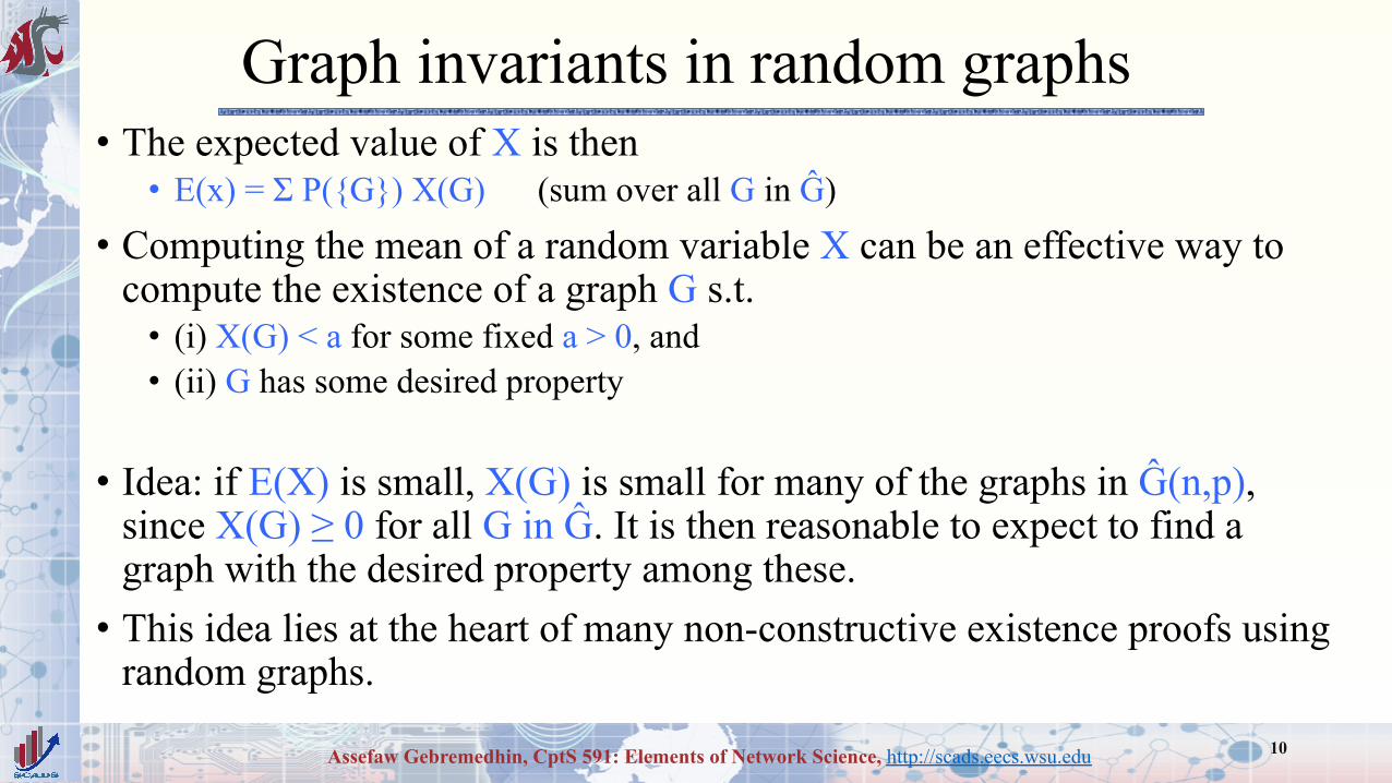
Graph invariants in random graphs • The expected value of X is then

•  E(x) = Σ P({G}) X(G) (sum over all G in Ĝ)

• Computing the mean of a random variable X can be an effective way to compute the existence of a graph G s.t. •  (i) X(G) < a for some fixed a > 0, and •  (ii) G has some desired property

•  Idea: if E(X) is small, X(G) is small for many of the graphs in Ĝ(n,p), since X(G) ≥ 0 for all G in Ĝ. It is then reasonable to expect to find a graph with the desired property among these. • This idea lies at the heart of many non-constructive existence proofs using

random graphs.

10


Markov’s Inequality

• Lemma 3: Let X ≥ 0 be a random variable on Ĝ(n,p) and a > 0. Then, P[X ≥ a] ≤ E(X)/a

• Proof:

E(X) = Σ P({G}) X(G) (sum over G in Ĝ(n,p))

≥ Σ P({G}) X(G) (sum over G in Ĝ(n,p) s.t. X(G)≥a)

≥ Σ P({G}) a (since X(G) ≥ a)

= P[X≥a] a (since a is constant) Rewriting, P[X≥a] ≤ E(X)/a

11


The Probabilistic Method

• Basic Idea: • To prove the existence of an object with some desired property, define a

probability space on some larger class of objects, and then show that an element of this larger space has the desired property

•  Illustrate using proof of Erdos’s theorem

12


Properties of almost all graphs and Phase transition

• Many results concerning “almost all graphs” have the common feature that the value of p (in the space Ĝ(n,p)) plays no role. • How could this happen?

• Then, what happens if p is allowed to vary with n?

13


Phase transition

14

p =p(n)

G in Ĝ (n,p)


Phase transition

15

p =p(n)

n-2

G a.s. has no edges G in Ĝ (n,p)


Phase transition

16

p =p(n)

n-2

n-3/2

G a.s. has no edges

G acquires more and more edges

Every component in G a.s. has at least two vertices

G in Ĝ (n,p)


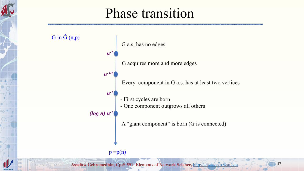
Phase transition

17

p =p(n)

n-2

n-3/2

n-1

(log n) n-1

G a.s. has no edges



-  First cycles are born -  One component outgrows all others

A “giant component” is born (G is connected)

G in Ĝ (n,p)


Phase transition

18

p =p(n)

n-2

n-3/2

n-1

(log n) n-1

(1+e) (log n) n-1

G a.s. has no edges



-  First cycles are born -  One component outgrows all others

A “giant component” is born (G is connected)

G a.s. has a Hamilton cycle

G in Ĝ (n,p)


Random graphs vs real-world networks

• Degree Distribution • Average Path Length • Clustering Coefficient

We will look at these in next lecture

19

random graphs - washington state university€¦ · graph invariants in random graphs • the...

Documents