random field characterisation of stress-normalised cone penetration testing parameters

Uzielli, M., Vannucchi, G. & Phoon, K. K. (2005). Geotechnique 55, No. 1, 3–20

3

Random field characterisation of stress-normalised cone penetrationtesting parameters

M. UZIELLI ,* G. VANNUCCHI* and K. K. PHOON†

Random field modelling of soil variability allows signifi-cant statistical results to be inferred from field data;moreover, it provides a consistent framework for incor-porating such variability in reliability-based design. Conepenetration testing (CPT) is increasingly appreciatedbecause of its near-continuity and repeatability. Stress-normalised CPT parameters are included in widely usedengineering procedures. Nonetheless, the results of varia-bility analyses for these parameters are surprisinglylimited. This paper attempts to characterise normalisedcone tip resistance (qc1N) and friction ratio (FR) rigor-ously using a finite-scale weakly stationary random fieldmodel. It must be emphasised that inherent soil variabil-ity so determined strictly refers to the variability of themechanical response of soils to cone penetration. Thevariability of soil response potentially depends on thefailure mode (shear for sleeve friction or bearing for tipresistance) and most probably on the volume of soilinfluenced (averaging effect). To investigate spatial varia-bility, 70 physically homogeneous CPT profiles were firstidentified from 304 soundings (subdivided into five regio-nal sites) and subsequently assessed for weak stationarityusing the modified Bartlett test. Only 40 qc1N profiles and25 FR profiles were deemed sufficiently homogeneousfrom both physical and statistical considerations for thescales of fluctuations to be valid and for estimation of thecoefficient of variation of inherent soil variability. Themajority of the acceptable profiles were found in sandysoils. The remaining profiles are in fine-grained soils,with a few in intermediate soils. Trends in the estimatedrandom field parameters indicate that qc1N is morestrongly autocorrelated than FR, probably because qc1N isinfluenced by a larger volume of soil around the cone tip,and that the mechanical response of cohesionless soils tocone penetration is significantly more variable and erra-tic than that of cohesive soils. Comparison with literaturedata indicates that normalisation leads to a decrease inthe scale of fluctuation for cone tip resistance and areduction in the coefficient of variation. A tentativeexplanation is that normalisation tends to minimise sys-tematic in situ effects that are explainable by physicalcauses.

KEYWORDS: in situ testing; numerical modelling and analysis;site investigation; soil classification; statistical analysis; theor-etical analysis

La modelisation aleatoire sur le terrain de la variabilited’un sol permet de deduire des resultats statistiques sig-nificatifs d’apres les donnees de terrain ; de plus, elle donneun cadre de travail constant permettant d’incorporer unetelle variabilite dans une conception basee sur la fiabilite.L’essai de penetration de cone (CPT) est de plus en plusapprecie en raison de sa quasi-continuite et reproductibi-lite. Les parametres CPT normalises du point de vue de lacontrainte sont inclus dans des procedures d’ingenierie tresutilisees. Neanmoins, les resultats des analyses de variabi-lite pour ces parametres sont etonnamment limites. Cetexpose essaie de caracteriser rigoureusement la resistancede la pointe de cone normalisee (qc1N) et le taux de friction(FR) en utilisant un modele de champs aleatoire faiblementstationnaire a echelle finie. Il faut souligner que la variabi-lite inherente du sol ainsi determine se rapporte stricte-ment a la variabilite de la reponse mecanique des sols a lapenetration des cones. La variabilite de la reponse du soldepend potentiellement du mode de defaillance (cisaille-ment pour friction de manche ou frottement pour laresistance de pointe) et plus probablement du volume desol influence (effet de moyenne). Pour etudier la variabilitespatiale, 70 profiles CPT physiquement homogenes ont eted’abord identifies parmi 304 sondages (subdivises en cinqsites regionaux) et ensuite etudies pour trouver la station-narite faible en utilisant l’essai de Bartlett modifie. Seule-ment 40 profiles qc1N et 25 profiles FR ont ete jugessuffisamment homogenes du point de vue physique etstatistique pour que les echelles de fluctuations soientvalables et pour estimer le coefficient de variation de lavariabilite inherente du sol. La majorite des profils accep-tables ont ete trouves dans des sols sableux. Les profilsrestants sont dans des sols a grains fins et quelques-unsdans des sols intermediaires. Les tendances des parametresde champs aleatoire estimes indiquent que qc1N est plusfortement auto-correle que FR, probablement parce queqc1N est influence par un plus gros volume de sol autour dela pointe du cone et que la reponse mecanique des sols noncohesifs a la penetration de cone est bien plus variable eterratique que celle des cols cohesifs. La comparaison avecles donnees publiees indique que la normalisation mene aune diminution de l’echelle de fluctuation pour la resis-tance a la pointe du cone et a une reduction du coefficientde variation. Nous tentons de l’expliquer par le fait que lanormalisation tend a minimiser les effets systematiques in-situ qui peuvent etre expliques par des causes physiques.

INTRODUCTIONThe importance of variability analysis is increasingly recog-nised in geotechnical engineering as reliability-based meth-

ods of varying degrees of sophistication are graduallyforming the basis for the calibration of new design codes.Notable examples include the Canadian Highway BridgeDesign Code (Green & Becker, 2001) and the AASHTOLRFD Bridge Design Specifications for Substructure Design(Withiam, 2003). Kulhawy & Phoon (2002) provided adetailed account of the development of geotechnical designcodes in recent years. Several models for geotechnicalvariability have been proposed in the literature (e.g. Baecher,1986; Orchant et al., 1988; Phoon & Kulhawy, 1999a,1999b). The aims of these models are (a) to identify the

Manuscript received 23 April 2004; revised manuscript accepted 30September 2004.Discussion on this paper closes on 1 August 2005, for furtherdetails see p. ii.* Department of Civil Engineering, University of Florence, Italy.† Department of Civil Engineering, National University of Singa-pore.

factors that contribute to overall variability, and (b) toevaluate the magnitude of each source of uncertainty. Varia-bility models, though presented using different terminolo-gies, basically identify inherent soil variability, measurementerror and transformation uncertainty as the primary sources.Inherent soil variability results primarily from natural geolo-gic processes that form and continuously modify the soilmass in situ. Measurement error arises from equipment,procedural-operator, and random testing effects. Equipmenteffects result from inaccuracies in the measuring devices andvariations in equipment geometries and systems employedduring testing. Procedural-operator effects originate fromlimitations in test standards and the way they are followed.Random testing error refers to (a) the remaining scatter inthe test results that is not assignable to specific testingparameters and is not caused by inherent soil variability, and(b) statistical uncertainty or sampling error that result fromlimited amounts of information. Transformation uncertaintyis introduced when field or laboratory measurements aretransformed into design soil properties using theoretical,semi-empirical or empirical models. These components areassumed to be uncorrelated. Such a hypothesis is important,as it justifies separate treatment of soil variability and testuncertainty (e.g. Agterberg, 1970; Orchant et al., 1988).

This paper focuses on the inherent variability of stress-normalised cone penetration test (CPT) measurements. Ingeneral, CPT measurements are ideal for assessing inherentsoil variability because a large volume of near-continuous datacan be collected in a cost-effective way, the test has goodrepeatability, the equipment is highly standardised, and theprocedure is well defined and almost independent of theoperator. Numerous researchers, such as Alonso & Krizek(1975), Tang (1979), Nadim (1986), Campanella et al. (1987),Wu et al. (1987), Reyna & Chameau (1991), Kulhawy et al.(1992), Fenton (1999), Phoon et al. (2003) and Elkateb et al.(2003a, 2003b), have assessed inherent soil variability usingthe CPT. However, results pertaining to stress-normalised CPTparameters are surprisingly limited. It is known that in-situstress states such as confining stress and stress history influ-ence CPT data quite significantly, and fairly reliable methodsfor stress normalisation have been proposed. Normalised CPTparameters are included in several widely used correlations forestimation of engineering parameters (in-situ stress state, stresshistory, strength, compressibility) and liquefaction susceptibil-ity evaluation. Moreover, normalised cone tip resistance andsleeve friction are key parameters in CPT-based soil classifica-tion systems (e.g. Robertson, 1990). Hence it may be possibleto relate inherent soil variability to soil type more directly. Itmust be emphasised that inherent soil variability so determinedstrictly refers to the variability of the mechanical response ofsoils to cone penetration. The variability of soil responsepotentially depends on the failure mode (shear for sleevefriction or bearing for tip resistance) and most probably on thevolume of soil influenced (averaging effect). A systematiccomparison of normalised cone tip resistance and sleeve fric-tion is undertaken in this study in terms of stationarity (orstatistical homogeneity) assessment, scale of fluctuation, andcoefficient of variation. Results reported in this study are basedon 70 physically homogeneous CPT profiles identified from304 soundings at various Turkish and North American sites.Soil types found at these sites cover zones 3 to 6 in theRobertson (1990) soil classification chart: that is, clay, siltyclay, clayey silt, sandy silt, silty sand, to clean sand.

DATABASENormalised CPT parameters

Various techniques for normalising CPT measurements forvertical stress are available. The normalised, dimensionless

cone penetration resistance (qc1N) proposed by Robertson &Wride (1998) is adopted in this study:

qc1N ¼ qc

Pa2

� �CQ (1)

where qc is the measured cone tip penetration resistance;CQ ¼ Pa=� 9v0ð Þn

is a correction for overburden stress; thevariable stress exponent n takes values of 0.50, 1.00 and0.70 for cohesionless, cohesive and intermediate soils re-spectively; � 9v0 is the effective vertical stress; Pa is areference pressure in the same units as �9v0 (i.e. Pa ¼100 kPa if � 9v0 is in kPa); and Pa2 is a reference pressure inthe same units as qc (i.e. Pa2 ¼ 0.1 MPa if qc is in MPa).An upper bound of CQ ¼ 1.7 is recommended for data atshallow depths (Youd et al., 2001). The normalised frictionratio is given by (Wroth, 1984):

FR ¼ 100f s

qc � �v0

(2)

where fs is the measured sleeve friction and �v0 is the totalvertical stress (qc, fs and �v0 in the same units). Owing tothe nature of soil formation and deposition processes, thevertical and horizontal correlation structures in soil proper-ties are generally anisotropic, with greater variability in thevertical direction. Here, inherent variability of qc1N and FR

is addressed only in the vertical direction: thus the results ofthe present study do not apply to the horizontal direction.

Identification of homogeneous soil unitsThe identification of homogeneous soil units is an impor-

tant prerequisite for variability analyses, as the correlationstructure of soil properties is potentially dependent on soiltype (in terms of composition and behaviour). Also, theassumption of statistical homogeneity—necessary for theapplication of statistical techniques—is not likely to applyunless the investigated volume of soil is fairly uniform incomposition or behaviour (Fenton, 1999). As CPT providesdirect information regarding the mechanical response of soilto penetration, homogeneity could also be assessed in amore fundamental way in relation to soil behaviour, ratherthan simply based on composition.

For the present study, preliminary selection of CPT datawas performed among a large number of soundings con-ducted at Turkish and North American sites. Five regionalsites were defined on the basis of geographical location andsource database:

(a) greater Oakland, CA, area (Alameda and Oaklandcounties) (hereinafter OAK)

(b) palaeoliquefaction sites in mid-America earthquakeregions (hereinafter MAE) (Collierville, TN; Dudley,MO; Marked Tree, AR; Memphis, TN; Mud Island,TN; Opelika, AL; St Louis, MO; Wilson, AR; WolfRiver, TN; Wyatt, MO)

(c) Texas A&M University site (TXS)(d) liquefaction sites in the Adapazari area, Turkey (ADP)(e) Treasure Island, in the San Francisco Bay area (TSI).

Data from OAK were collected as part of the USGS Earth-quake Hazards Program, and are available at http://quake.wr.usgs.gov/prepare/cpt/; MAE data were collected by theGeorgia Tech In-Situ Testing Group (http://www.ce.gatech.edu/�geosys/Faculty/Mayne/Research/index.html); TXS andTSI soundings were conducted at Texas A&M and TreasureIsland NGES sites respectively (http://www.unh.edu/nges/);and ADP data are available on the PEER website (http://

4 UZIELLI, VANNUCCHI AND PHOON

peer.berkeley.edu/turkey/adapazari/). The above data werescreened based on the following criteria:

(a) The measurement interval is less than 0.05 m.(b) Reliable measurement of groundwater level is reported.(c) The length of the sounding is at least 10 m.

The first criterion ensures that there is sufficient resolutionfor accurate variability assessment (e.g. Jaksa et al., 1997;Cafaro & Cherubini, 2002). The second is a necessarycondition for the calculation of qc1N and FR. The thirdensures that the record length is long enough for stationarityassessment (a stationary process is theoretically infinite inlength) and the sample size is large enough for meaningfulstatistical treatment. A total of 304 soundings were consid-ered adequate for analysis based on the above selectioncriteria.

Homogeneous soil units (HSU) were identified from theselected soundings using a statistical moving window proce-dure proposed by Uzielli (2004). The procedure involvedconverting the data to normalised form as given by equations(1) and (2) and applying a moving window on profiles ofqc1N, FR and the soil behaviour classification index, Ic (e.g.Robertson & Wride, 1998), for statistical identification. Thesoil behaviour classification index maps the usual two-dimen-sional CPT-based soil behaviour classification zones onto aone-dimensional scale, and is calculated from qc1N and FR:

Ic ¼ [(3:47 � log qc1N)2 þ (1:22 þ log FR)2]0:5 (3)

The scale is shown in Fig. 1. Each moving window is madeup of two semi-windows of equal height above and below acentre point. At each centre point (identified by its depth zc),the mean, standard deviation and coefficient of variation(COV) were calculated for data lying in the interval zc �Wd/2 < z < zc + Wd/2, corresponding to the upper and lowerlimits of the moving window of height Wd ¼ 1.50 m. Theheight of the moving window was set on the basis of pastresearch (e.g. Campanella et al., 1987; Wickremesinghe,1989; Lunne et al., 1997) and calibration of results withavailable borehole logs (Uzielli, 2004).

HSUs are essentially identified by delineating soundings

into sections where COV(log qc1N) and COV(Ic) are less than0.1 over at least 4.50 m. Harr (1987) proposed a value of0.1 for COV as the upper limit for ‘low dispersion’ in soilproperties. Two additional conditions were imposed to ensurethat there are sufficient data points for meaningful statisticalanalysis and log(qc1N) and Ic do not exhibit gradual changeswith depth. A total of 70 HSUs were identified from the 304selected soundings. Details of the CPT database and theidentification procedure are given elsewhere (Uzielli, 2004).

To provide a concise overview of the 70 HSUs, the meanvalues of qc1N and FR and their corresponding standarddeviations are plotted on the Robertson (1990) chart aspoints and error bars respectively (Fig. 1). The ability of themoving window procedure to identify homogeneous soilunits was assessed by observing that the mean value of thecoefficients of variation of Ic in the HSUs was 0.02, and thatvalues in no case exceeded 0.10. Fig. 1 shows that theidentified HSUs cover a wide range of soil types (zones 3 to6). It may also be observed in Fig. 1 that the standarddeviation of qc1N and FR increases approximately fromcategory 3 to 6, i.e. from clay to sand, indicating that CPTprofiles are more variable in cohesionless soils. This mayalso be seen in Fig. 2, in which typical profiles of qc1N andFR are plotted against depth for a cohesive soil (CHS)hsu003, classified in zone 3, and a cohesionless soil (CHL)hsu010, classified in zone 6. Fig. 3 illustrates the subdivisionof HSUs by regional site in the Robertson chart. As shownin Table 1, the mean values of qc1N and FR of the 13 HSUsfrom OAK sites fall in zones 3, 4, 5 and 6; the 27 HSUsfrom MAE in zones 4 and 6; the 6 HSUs from TXS inzones 4 and 5; the 18 HSUs from ADP in zones 3 and 6;and the 6 HSUs from TSI in zone 3 only. Hence it ispossible to study trends based on geographic location andsoil type.

RANDOM FIELDInherent soil variability may be modelled using finite-scale

stochastic processes, which assume limited spatial correla-tion, or by fractal processes, which admit significant linger-

��

��

��

��

�

� ��

� ��

� ��

��

�

��

��

� ��

�

��

��

�

�

�

�

�

�

�

�� !

"��#�$��%��&��

"��#�$��%�'��

��(� "��#�$��%��&�

�

�

�

�

�

�

�

"��$�)��(��

*�(��+�&��

,��)��

"��-�%��+��

"��-�%��+��

,��)��

.��$��

/��

/��)��(��

��&&�0

��

��

��

��

��

��

��&&�0

��&&�0

Fig. 1. Mean values and standard deviations of homogeneous soil units as viewed within the context of Robertson’s(1990) soil classification chart, with superimposed boundaries of soil behaviour type index, Ic

RANDOM FIELD CHARACTERISATION OF STRESS-NORMALISED CPT PARAMETERS 5

ing correlation over large distances. CPT measurements arenot truly point measurements, but are representative para-meters of the extent of the zone in which soil failure occursdue to penetration; hence small-scale variations may not bedetectable. Moreover, previous research (e.g. Fenton, 1999;Phoon et al., 2003) suggests that it is difficult to distinguishbetween finite-scale and fractal models over a finite samplingdomain. Thus a finite-scale approach is possibly more suita-ble.

In this study, inherent soil variability is modelled as azero-mean weakly stationary random field with finite-scalecorrelation structure (Vanmarcke, 1983). This random fieldis added to a trend function that is assumed to be determi-nistic in nature. It should be emphasised that soil propertiesare not ‘random’ in the sense that they are intrinsicallyunknown, but are modelled as ‘random’ because it ispractically impossible to obtain measurements at all points.The mathematical and statistical techniques commonly usedto treat stochastic processes are then useful to describespatial variations in a parsimonious and concise way(Baecher & Christian, 2003).

DecompositionThe ‘real’ value (i.e. neglecting measurement error) of a

geotechnical property [�(z)] may be decomposed into asmoothly varying trend function [t(z)] and a fluctuatingcomponent [w(z)] representing the inherent soil variability:

�

�

�

�

,12

,1"

��

��

��

�

� ��

��

�!

��

��

��

�

,12

,1"

�� !

�

�

��

��

��

� ��

��

�!

,12� #�%��!

3�� !��

,*/� ��!��

3��!��

,*/� ��!��

,1"� #�%��!

3�� !��

,*/� ��!��

3�� !��

,*/� ��!��

�

�

�

,12 ,1"

� ��

��

Fig. 2. Representative examples of cohesionless (CHL) and cohesive (CHS) behaviour HSUs: (a) plot on Robertson’s(1990) chart; plots of (b) qc1N and (c) FR against relative depth, zt (depth from top of HSU) with linear trends

�

�

�

�

�

�

�

*4534678"49:7";

� ��

��

� ��

�

� ��

�

� ��

��

�

��

��

�� 3�� !��

��

��

��

�

3��

��

��!

Fig. 3. Categorisation of HSUs by regional site (after Robertson,1990)


Table 1. Number of best-fit ACMs for HSUs categorised by soil behaviour zone and regional site (qc1N and FR)

Reg. Soil qc1N FRsite zone

SNX CSX SMK SQX TotalSTAT

NST NAPP Total(reg. site)

SNX CSX SMK SQX TotalSTAT

NST NAPP Total(reg. site)

OAK 3 0 0 0 0 0 1 1 2 0 0 0 0 0 1 1 24 1 0 1 0 2 1 1 4 0 1 0 0 1 1 2 45 0 0 0 0 0 3 1 4 0 1 0 0 1 2 1 46 2 0 1 0 3 0 0 3 0 0 1 0 1 1 1 3

Total OAK 3 0 2 0 5 5 3 13 0 2 1 0 3 5 5 13MAE 3 0 0 0 0 0 0 0 0 0 0 0 0 0 0 0 0

4 0 0 2 0 2 1 1 4 1 0 0 0 1 2 1 45 0 0 0 0 0 0 0 0 0 0 0 0 0 0 0 06 0 3 6 10 19 2 2 23 2 2 7 0 11 8 4 23

Total MAE 0 3 8 10 21 3 3 27 3 2 7 0 12 10 5 27TXS 3 0 0 0 0 0 0 0 0 0 0 0 0 0 0 0 0

4 0 0 0 1 1 0 2 3 0 2 0 0 2 1 0 35 0 0 1 0 1 2 0 3 0 0 0 0 0 1 2 36 0 0 0 0 0 0 0 0 0 0 0 0 0 0 0 0

Total TXS 0 0 1 1 2 2 2 6 0 2 0 0 2 2 2 6ADP 3 0 2 2 1 5 6 4 15 1 1 1 0 3 10 2 15

4 0 0 0 0 0 0 0 0 0 0 0 0 0 0 0 05 0 0 0 0 0 0 0 0 0 0 0 0 0 0 0 06 0 1 2 0 3 0 0 3 0 1 1 0 2 1 0 3

Total ADP 0 3 4 1 8 6 4 18 1 2 2 0 5 11 2 18TSI 3 1 2 1 0 4 0 2 6 2 0 1 0 3 1 2 6

4 0 0 0 0 0 0 0 0 0 0 0 0 0 0 0 05 0 0 0 0 0 0 0 0 0 0 0 0 0 0 0 06 0 0 0 0 0 0 0 0 0 0 0 0 0 0 0 0

Total TSI 1 2 1 0 4 0 2 6 2 0 1 0 3 1 2 640 16 14 70 25 29 16 70

RA

ND

OM

FIE

LD

CH

AR

AC

TE

RIS

AT

ION

OF

ST

RE

SS

-NO

RM

AL

ISE

DC

PT

PAR

AM

ET

ER

S7

� zð Þ ¼ t zð Þ þ w zð Þ (4)

where z is the depth coordinate. The importance of thedecomposition procedure has been recognised by manyresearchers; inappropriate removal of the deterministic trendcomponent from a measurement profile would result in abiased assessment of correlation. The choice of the trend tobe removed is a complex task as it affects the correlationstructure and the value of the statistical parameters describ-ing the random field (coefficient of variation and scale offluctuation). In addition, trend removal should at least resultin stationary residuals. Given the above considerations, it isimportant to limit trend functions to those that are consistentwith local geology and well-established principles of soilbehaviour in geotechnics. In the present study, the followingcriteria were taken into account in choosing the method oftrend removal:

(a) the existence of a physical motivation (e.g. Akkaya &Vanmarcke, 2003; Baecher & Christian, 2003)

(b) compatibility with available models for the estimationof random field parameters

(c) compatibility with the adopted stationarity assessmentcriterion.

Trend removal by linear least-squares regression analysiswas found to meet the above requirements. Linear trendremoval has been used in several variability studies (e.g.Campanella et al., 1987; Popescu et al., 1998; Elkateb et al.,2003a, 2003b; Phoon et al., 2003; Uzielli, 2004), thoughstress normalisation studies have shown that the variation ofvertical trends may take other forms, especially for cohe-sionless soils. Moreover, while such an approach may not befully consistent owing to the presence of correlated resi-duals, and, consequently, could lead to unconservative andbiased estimates (e.g. Agterberg, 1970; Campanella et al.,1987; Baecher, 1999; Fenton, 1999), its use seems appro-

priate here, mainly for two reasons. First, normalisation byvertical effective stress should account for systematic physi-cal effects on the soil profiles (e.g. overburden stress andstress history). Thus profiles of vertical stress-normalisedvariables of homogeneous soil units should no longer displaysignificant trends with depth beyond a simple first-orderlinear function. Second, it should be emphasised here thatthe more important goal is not to violate weak stationarity inthe resulting residuals or fluctuations, regardless of themethod of trend removal. Even though regression is notstrictly applicable to correlated residuals, it is possible toassess the impact of this inconsistency independently usingthe modified Bartlett test described below (Phoon et al.,2003). Fig. 4 shows an example HSU identified using thestatistical procedure described above. The performance ofthe identification procedure may be appreciated throughvisual examination of the aggregated data points in Fig.4(a). Profiles of qc1N, FR and Ic in the HSU and the lineartrends identified by regression are shown in Figs 4(b), 4(c)and 4(d) respectively.

Estimation of the scale of fluctuationIn finite-scale models, the scale of fluctuation (�) is a

concise indicator of the spatial extent of a strongly corre-lated domain. There are various curve-fitting and statisticaltechniques available in the geotechnical literature for theestimation of the autocorrelation model and scale of fluctua-tion (e.g. DeGroot & Baecher, 1993, Fenton, 1999). Asimple but robust approach is to estimate the sample auto-correlation function (ACF) using the method of moments, fita plausible theoretical autocorrelation model (ACM) to ACF,and evaluate the scale of fluctuation based on the modelparameter in the ACM.

The jth coefficient of the sample autocorrelation function

�

�

�

�

�

�

�

� ��

�

� ��

��

� ��

�

� ��

��

��

��

��

�

� ��

��

� � ��

�

�

�

�

��

��

��

�

� ��

�

�

�

�

��

��

��

�

�

�

�

�

��

��

��

� � ��

��

1">�?��#�� %��$�� 1">

�!

3�� !�� ,*/ ��!��

�!

3�� !��,*/ ��!��

�!

3�� !�� ,*/ ��!��

�!

Fig. 4. Example of identified HSU: (a) plot of complete HSU data points in Robertson’s (1990) chart; plots of (b) Ic, (c) qc1Nand (d) FR profiles against relative depth, zt (depth from top of HSU) with superimposed linear trends


(ACF) of the fluctuating component wi ¼ w(zi) (which is azero-mean stochastic process) is given by

RR � jð Þ ¼

Xnd� j

i¼1

wi � wiþ j

Xnd� j

i¼1

w2i

(5)

The ACF was calculated for separation distances �j ¼ j˜zcorresponding to j ¼ 1, 2, . . ., nd/4, as suggested by Box &Jenkins (1970), where nd is the number of data points in agiven profile and ˜z is the sampling interval. Various kindsof ACM have been employed in the geotechnical literatureto fit the ACF (e.g. Spry et al., 1988; DeGroot & Baecher,1993; Jaksa, 1995; Lacasse & Nadim, 1996; Fenton, 1999;Phoon et al., 2003). Spry et al. (1988) opined that there isno physical basis to prefer one ACM over another. In thisstudy, it was found that the following four ACMs weresufficient to fit sample ACFs derived from CPT data:

(a) single exponential (SNX)(b) cosine exponential (CSX)(c) second-order Markov (SMK)(d) squared exponential (SQX).

The analytical expressions of the four ACMs and theformulae relating the scales of fluctuation to the modelparameters are shown in Table 2.

To increase the reliability of the estimated �, Uzielli(2004) fitted the ACMs only to the initial part of the sampleACF with coefficients exceeding Bartlett’s limits:

rB ¼ 1:96ffiffiffiffiffind

p (6)

This guideline has been used by Spry et al. (1988) and ismotivated by the well-accepted fact that the estimated auto-correlation coefficients become less reliable with increasinglags, and are deemed not significantly different from zeroinside the range �rB (e.g. Priestley, 1981; Brockwell &Davis, 1991; Fenton, 1999). The coefficient of determination,R2, was recorded for each ACM fit. Only ACMs producingR2 . 0.9, with at least four initial autocorrelation coeffi-cients greater than rB to ensure the significance of the fit,were accepted. The procedure outlined above was applied toqc1N and FR profiles for all HSUs. Examples of best-fit forSNX, CSX, SMK and SQX ACMs to sample ACFs fromqc1N profiles are shown in Figs 5(a), 5(b), 5(c) and 5(d)respectively. It can be seen that the curves from the fourACMs display distinct shapes at low lags: hence, if the fit ofan ACM to a sample ACF is performed with emphasis onlow separation distances, the correlation between measure-ments in the volume of soil nearest to the cone (i.e. mostdirectly affected by penetration) assumes a relevant role inrandom field modelling as defined herein.

Modified Bartlett testAs stated previously, weak stationarity is an important

requisite for random field characterisation of soil properties.Weak stationarity cannot be verified in a strict sense over afinite length because longer scale fluctuation can bemistakenly identified as a non-stationary component

Table 2. Autocorrelation models and relations between scale of fluctuation andcharacteristic model parameters

Autocorrelation model Equation Scale of fluctuation

SNX R(�) ¼ exp(�kSNXj�j) � ¼ 2=kSNX

CSX R(�) ¼ exp(�kCSXj�j)cos(kCSX�) � ¼ 1=kCSX

SMK R(�) ¼ (1 þ kSMKj�j)exp(�kSMKj�j) � ¼ 4=kSMK

SQX R(�) ¼ exp[�(kSQX�)2] � ¼ffiffiffiffiffiffi�=

pkSQX

��&��"8,"8"35"@8

�� "8!�� ,"8!�� "35!�� "@8!��

3��%��$��1">��A��$��%��#��(�� !

��4,=��%��

� �� !

��

��

�

��

��

B� �

!

��&��"8,"8"35"@8

�� "8!�� ,"8!�� "35!�� "@8!��

3��%��$��1">��A��$��%��#��(�� !

��4,=��%��

� �� !

��

��

�

��

��

B� �

!

��&��"8,"8"35"@8

�� "8!�� ,"8!�� "35!�� "@8!��

3��%��$��1">��A��$��%��#��(�� !

��4,=��%��

� �� !

��

��

�

��

��

B� �

!

��&��"8,"8"35"@8

�� "8!�� ,"8!�� "35!�� "@8!��

3��%��$��1">��A��$��%��#��(�� !

��4,=��%��

� �� !

��

��

�

��

��

B� �

!

� � ��

� ��

Fig. 5. Example of best-fit case for: (a) SNX (hsu068); (b) CSX (hsu027); (c) SMK (hsu062); (d) SQX (hsu019) ACMs


(e.g. Agterberg, 1970; Baecher, 1999; Fenton, 1999; Phoonet al., 2003). Thus only local weak stationarity can beidentified. A profile is considered to be weakly stationary if(a) the mean is constant over a given spatial direction, and(b) the autocovariance is only a function of the separationdistance � j between observations.

Numerous researchers (e.g. Watson, 1967; Agterberg,1970; Fenton, 1999; Phoon et al., 2003) have noted that theapplication of classical statistical tests (e.g. statistical runstest, Spearman’s rank coefficient and Kendall’s tau test) tocorrelated data may result in biased assessments. The mod-ified Bartlett statistic procedure (MBS) was proposed byPhoon et al. (2003) with the aim of providing a morerational basis for rejecting the null hypothesis of stationarityin the correlated case. MBS has been shown to be morediscriminating than other traditional classical tests (Uzielli etal., 2004), as it (a) incorporates the correlation structure inthe underlying data, and (b) includes all the key assumptionsin geostatistical analysis (stationarity, choice of trend func-tion, and autocorrelation model). This generality is achievedby exploiting powerful digital simulation techniques forrandom fields. The MBS procedure neglects measurementand random testing errors: this assumption is acceptable forthe CPT, which has been shown to be largely operator-independent and to have very low random measurementerrors (e.g. Campanella et al., 1987; Kulhawy & Trautmann,1996; Jaksa et al., 1997).

In the MBS procedure, Bartlett statistics (basically theratio of variances in two contiguous segments) are computedby applying a moving window method to fluctuating profile.The test statistic is the peak value of the Bartlett statisticprofile (Bmax), and it is compared with a critical value (Bcrit)derived using simulation. The null hypothesis of stationarityin the variance is rejected at the customary 5% level ofsignificance if Bmax . Bcrit. This study basically follows theMBS procedure described by Phoon et al. (2003), withadditional steps introduced (fitting ACM to the initial part ofACF and rejecting ACM producing R2 , 0.9) to achievemore robust estimates for the scale of fluctuation. Theprocedure as revised by Uzielli (2004) will be referred to asMBSR hereon.

For data sets satisfying the condition of weak stationarity,the dimensionless coefficient of variation of inherent varia-bility (�) is obtained by normalising the standard deviationwith respect to the value of the linear trend function at themidpoint of the homogeneous soil unit under investigation(tM) (Phoon & Kulhawy, 1999a):

� ¼

ffiffiffiffiffiffiffiffiffiffiffiffiffiffiffiffiffiffiffiffiffiffiffiffiffiffiffiffiffiffi1

nd � 1

Xnd

i¼1

wi½ �2s

tM

(7)

STATIONARITY OF CPT SOUNDINGSWhile HSUs are defined in terms of homogeneity of both

qc1N and FR (corresponding to tight clusters in the Robertson(1990) chart), it should be emphasised that weak stationarity(or non-stationarity) of one parameter does not necessarilyimply the same assessment for the other. Cone tip resistanceand sleeve friction are profoundly different measurements, asthey are related to distinct aspects of soil behaviour (bearingcapacity and friction), and they are influenced by differentvolumes of penetrated soil (tip resistance being influencedby soils within a few diameters around the tip, and sleevefriction being affected only by soil adjacent to it).

Three outcomes are possible for each profile of qc1N orFR:

(a) MBSR is not applicable in its entirety, for one or moreof the following reasons: (i) R2 does not exceed 0.9 forany of the four ACMs shown in Table 2; (ii) one ormore of the dimensionless profile factors of the MBSprocedure (k, I1, I2), which depend on the scale offluctuation (�), sample spacing (˜z), and sample size(nd), fall outside the ranges established by Phoon et al.(2003).

(b) MBSR could be applied, but Bmax > Bcrit: thus theprofile is classified as non-stationary at 5% significancelevel.

(c) The MBSR procedure could be applied in its entirety,and at least one ACM satisfies the goodness-of-fit andstationarity criteria at the 5% level. If more than oneACM satisfy the above conditions, the scale offluctuation resulting from the ACM with the maximumR2 is adopted.

Only results from case (c) are analysed further and discussedin detail below. Note that 40 and 25 values of � wereaccepted for qc1N and FR respectively, out of values from 70possible HSUs. Out of the 40 MBSR-stationary qc1N profiles,five belonged to OAK sites, 21 to MAE, two to TXS, eightto ADP, and four to TSI (Table 1). Out of the 25 MBSR-stationary FR profiles, three belonged to OAK sites, 12 toMAE, two to TXS, five to ADP, and three to TSI.

Assessment of weak stationarityFigures 6(a) and 6(b) show the best-fit ACM for each

HSU (if MBSR-stationary) for qc1N and FR respectively.Table 1 summarises the distribution of HSUs according tothe best-fit ACM (SNX, CSX, SMK or SQX) if they arestationary. The numbers of cases that are non-stationary ornot amenable to MBSR are also noted. In addition, station-ary (STAT), non-stationary (NST) and non-applicable cases(NAPP) are further categorised according to the soil zone inwhich the mean values of FR and qc1N in the HSU arelocated in the Robertson (1990) chart.

It is evident from Table 1 that FR is not appropriate forstationary assessment as the rate of rejection of the station-ary hypothesis is too high (25 stationary versus 29 non-stationary). Although physical homogeneity does not neces-sarily correspond to statistical homogeneity (or stationarity),one does expect a stronger correlation such as that producedby qc1N (40 stationary versus 16 non-stationary). It is wellknown that sleeve friction is much less reliable than tipresistance. DeJong and Frost (2002) demonstrated that moreaccurate soil characterisation could be achieved by measur-ing sleeve friction at a larger distance behind the tip (.0.35 m). It is quite surprising that most of the non-stationaryHSUs fall in zone 3, which corresponds to clays and siltyclays. A closer examination reveals that such evidence maybe due to the fact that although CPT profiles in sands aremore variable than those in clays, the latter occasionallyshow large jumps embedded in predominantly smaller fluc-tuations (see Fig. 2), and some of these spikes result in verylarge—though isolated—peaks in Bartlett statistics. Non-applicability of the MBSR procedure resulted in most casesfrom insufficient reliability of ACM fitting: out of the 14NAPP HSUs for qc1N, 12 were not amenable to MBSRowing to insufficiently high R2, while only two did not meetthe range of dimensionless MBS factors. The correspondingbreakdown for the 16 NAPP FR HSUs is 15 and onerespectively.

For qc1N, the SMK and SQX models are more common,particularly in sandy soils (zone 6). Incidentally, SMK andSQX are the ACMs that provide higher autocorrelation coef-ficients in the initial part of the ACF (i.e. those correspond-


ing to smaller separation distances). For FR, the SQX modeldoes not provide the best fit in any soils. These observationsare compatible with the fact that the cone tip resistance isinfluenced by a larger volume of soil, and hence induceslarger correlations at short lags. Interestingly, all qc1N andFR profiles with mean values falling within the normallyconsolidated area of zones 3 and 4 were not amenable toMBSR or were deemed non-stationary (NAPP or NST inFigs 6(a) and 6(b)). More data are needed to clarify thepotential role of in-situ soil state and stress history in soilvariability.

SECOND-MOMENT STATISTICS OF CPT SOUNDINGSA random field may be described concisely in the second-

moment sense by the scale of fluctuation and the coefficientof variation. A careful study of these important statistics ispresented below. First, it will be verified that the statisticsare not biased by the number of CPT measurement points

within each HSU, the CPT measurement interval, and thebest–fit autocorrelation model (ACM). Second, the statisticscomputed from qc1N and FR are studied separately byplotting them against mean qc1N and mean FR respectively.The effect of soil type is then interpreted using theRobertson (1990) chart, which considers mean qc1N andmean FR jointly. Finally, if sufficient data are available, site-specific effects not explainable by mean qc1N, mean FR, andsoil type are highlighted.

Vertical scale of fluctuationPossible bias produced by sample size (i.e. the number of

measurements in an HSU) and spacing (i.e. CPT measure-ment interval) was first investigated by plotting the estimatesfor qc1N (Fig. 7(a)) and FR (Fig. 7(b)) against sample size,with data points categorised by measurement interval. Nosignificant trends are visible. Hence the estimates of correla-tion distance for MBSR-stationary HSUs are considered tobe unbiased in terms of sample size and spacing.

The scales of fluctuation (�) for each MBSR-stationaryprofile are plotted against mean qc1N (Fig. 8(a)) and meanFR (Fig. 8(b)) according to the best-fit ACM. The scales offluctuation computed by one ACM do not rank consistentlyabove or below the others. This may not come as a surprisegiven that � is defined to make different ACMs comparable(Vanmarcke, 1983). Table 3 shows second-moment statistics(mean and coefficient of variation) for the scale of fluctua-tion of qc1N and FR categorised by best-fit ACM and soiltype (i.e. location of the mean values of qc1N and FR in theRobertson (1990) chart). On average, the scale of fluctuationof qc1N is higher than the scale of fluctuation of FR (Table3). The former lies between 0.13 and 1.11 m, with only twovalues below 0.2 m and one value above 1.0 m, whereas thelatter lies between 0.12 and 0.6 m. The overall mean valuesare 0.70 m for �(qc1N) and 0.39 m for �(FR), with lowerdispersion for qc1N (COV ¼ 0.28) than for FR (COV ¼ 0.40).The stronger correlation structure of qc1N may find a physi-cal basis in the fact that sleeve friction measurements and,consequently, FR are more erratic than cone tip resistancemeasurements. This is to be expected, given that qc1N isinfluenced by a volume of soil around the cone tip that islarger than the sampling interval. Hence a few continuous

"8,"8"35"@8"74::

��

3��

�!

��

��

��

�

3��

��

�

�

�

�

�

�

�

��

��

� ��

��

��

� ��

� ��

"8,"8"35"@8"74::

��

3��

�!

��

��

��

�

3��

��

�

�

�

�

�

�

�

��

��

� ��

��

��

� ��

� ��

��

��

Fig. 6. Results of MBSR stationarity assessment for (a) qc1N and(b) FR profiles (after Robertson, 1990)

��

� ��

�!

��

��

��

�

� � �

�!��

��

��

�!

��

��

��

�

� �

�!��

Fig. 7. Plots of data numerosity of HSUs against scale offluctuation for: (a) qc1N; (b) FR


values of qc1N are basically affected by almost the samevolume of soil as the cone penetrates. In addition, morereliable sleeve friction measurements are apparently possibleif they are obtained further behind the tip (DeJong & Frost,2002). This suggests that present sleeve friction measure-ments from standard cones possibly contain more noise,which further weakens the correlation.

Figure 9 is similar to Fig. 8, except that the data pointsare differentiated according to the regional site. Note thatdifferent regional sites contain different proportions of dif-ferent soil types, as shown in Table 4. For example, almostall MAE HSUs are soil type 6, all TSI HSUs are soil type3, and OAK HSUs cover soil types 4 and 6. Before attribut-ing any trends in Fig. 9 to site-specific effects, it is probablymore reasonable to see whether these trends are explainableby differences in soil types or, more specifically, by differ-ences in the mean qc1N and FR.

It is quite evident from Fig. 9(a) that the lower and upperbounds of �(qc1N) generally increase with increasing meanqc1N when all the regional sites are considered together. Thisis also shown in the last row of Table 4. The mean scale offluctuation for qc1N also exhibits this increase, but not asclearly given the large scatter. This trend can also bediscerned within a regional site, particularly for data fromADP and MAE (Table 4).

The cluster of four TSI data points with qc1N , 10 areclassified as soil type 3 and probably belong to the YoungBay Mud layer (Fig. 9(a)). The range of �(qc1N) (0.13–0.23 m) for this cluster lies entirely below those of the otherregional sites. For instance, the scales of fluctuation for ADPHSUs belonging to soil type 3 range between 0.28 and0.64 m (Table 4). The range of �(qc1N) values at TSI wascomputed using different best-fit ACMs (1 SNX, 2 CSX and1 SMK) as shown in Table 1. Hence these low values arenot caused by the choice of a particular ACM. This effect isalso exhibited by �(FR) at the same regional site, as therange 0.13–0.28 m is lower than 0.26–0.45 m for HSUsconsisting of soil type 3 at ADP. Hence it would appear thata site-specific effect is present at TSI. It is also possible tocompare results for soil type 6 from OAK, MAE, and ADP.Unlike the case for TSI, there is no strong evidence tosuggest that a site-specific effect is present here, given thelarge scatter and unequal sample sizes at the three regionalsites.

The sample sizes for �(FR) are smaller, and the trends inFig. 9(b) should be interpreted with this caveat in mind.Overall, the lower and upper bounds appear to decrease

slightly with increasing mean FR. Note that soil type 3 hashigh FR but low qc1N, whereas the reverse is true for soiltype 6 in the Robertson (1990) chart (Fig. 6). Hence theabove observation actually supports the opposing trend ob-served for �(qc1N) data, which essentially indicates thatcohesionless soils are somewhat more correlated than cohe-sive soils. The negative trend for �(FR) is, however, muchweaker than the increasing trend for �(qc1N). This is alsocompatible with the results of past research (e.g. Teh &Houlsby, 1991), which indicate that the extent of the failurezone increases with increasing shear strength and stiffness:thus the influence zone affecting cone tip resistance is largerin sand, whereas sleeve friction is affected only by theadjacent soil regardless of soil type. A possible site-specificeffect can be seen in Fig. 9(b): the MAE soil type 6 datapoints plot above the ADP data points of the same soil typein the mean FR range between 0.6% and 0.9%. However, itshould be noted that there are 11 data points for MAE andonly two data points for ADP (Table 4). The single OAKsoil type 6 data point agrees with the MAE cluster, althoughthe mean FR is about 2%.

It is interesting to examine the effect of normalisation onthe scale of fluctuation through comparison with results fromthe literature (e.g. Appendix A in Phoon et al. 1995). Phoon& Kulhawy (1999a) observed a range of 0.1–2.2 m with anaverage value of 0.9 m for the non-normalised cone tipresistance (qc) from seven studies covering both sands andclays. Cafaro & Cherubini (2002) estimated the averagevalues of the scale of fluctuation of linearly detrended qc

data of two Italian clays as 0.40 and 0.57 m. Elkateb et al.(2003b) estimated scales of fluctuation of qc ranging from0.37 to 0.80 m for four soil layers classifiable as types 5 and6 in the Robertson (1990) chart. For strict comparison withother literature data, the type of trend removed should bespecified, as the removal of higher-order polynomial trendsresults in a decrease in the scale of fluctuation (e.g. Jaksa etal., 1997; Phoon et al., 2003). In addition, it is known thatestimates of scales of fluctuation are usually not very precise(besides trend removed, they depend on how ACF is eval-uated, choice of ACM, fitting criteria, etc.). Nevertheless, abroad comparison seems to indicate that the scale of fluctua-tion for qc1N is comparable to or shorter than that for qc.This observation is compatible with the fact that normal-isation tends to minimise systematic physical in-situ effects(depositional processes and confining pressure) that mayintroduce subtle trends, and hence longer correlation lengthsin the data. Literature results for normalised and non-nor-

"8

,"8

"35

"@8

��

��

��

��

��

�

��

� ��

!��

� �� 3�� !

�!

"8

,"8

"35

"@8

��

��

��

��

��

�

��

� �

�!��

�� 3�� !��

�!

Fig. 8. Scale of fluctuation against mean value in HSU for MBSR-stationary HSUs, categorised by best-fit ACM: (a) qc1Nprofiles; (b) FR profiles


Table 3. Vertical scale of fluctuation (�) for MBSR-stationary HSUs categorised by best-fit ACM and soil behaviour zone

ACM qc1N FR

Zone Overall (ACM) Zone Overall (ACM)

3 4 5 6 3 4 5 6

SNX No. HSUs 1 1 0 2 4 3 1 0 2 6Range: m 0.19 0.82 – 0.98–1.11 0.19–1.11 0.13–0.45 0.40 – 0.53–0.58 0.13–0.58Mean: m 0.19 0.82 – 1.04 0.77 0.29 0.40 – 0.55 0.39COV – – – 0.06 0.46 0.45 – – 0.05 0.38

CSX No. HSUs 4 0 0 4 8 1 3 1 3 8Range: m 0.13–0.64 – – 0.56–0.79 0.13–0.79 0.35 0.12–0.49 0.60 0.19–0.59 0.12–0.60Mean: m 0.32 – – 0.68 0.50 0.35 0.25 0.60 0.39 0.36COV 0.59 – – 0.14 0.46 – 0.68 – 0.42 0.51

SMK No. HSUs 3 3 1 9 16 2 0 0 9 11Range: m 0.22–0.50 0.33–0.96 0.35 0.39–0.97 0.22–0.97 0.20–0.26 – – 0.26–0.60 0.20–0.60Mean: m 0.37 0.67 0.35 0.74 0.63 0.23 – – 0.46 0.42COV 0.30 0.39 – 0.25 0.38 0.13 – – 0.25 0.33

SQX No. HSUs 1 1 0 10 12 0 0 0 0 0Range: m 0.28 0.99 – 0.39–0.84 0.28–0.99 – – – – –Mean: m 0.28 0.99 – 0.61 0.62 – – – – –COV – – – 0.28 0.35 – – – – –

Overall (zone) No. HSUs 9 5 1 25 40 6 4 1 14 25Range: m 0.13–0.64 0.33–0.99 0.35 0.39–1.11 0.13–1.11 0.13–0.45 0.12–0.49 0.60 0.19–0.60 0.12–0.60Mean: m 0.32 0.76 0.35 0.70 0.61 0.28 0.29 0.60 0.46 0.39COV 0.48 0.31 – 0.28 0.42 0.37 0.56 – 0.28 0.40

RA

ND

OM

FIE

LD

CH

AR

AC

TE

RIS

AT

ION

OF

ST

RE

SS

-NO

RM

AL

ISE

DC

PT

PAR

AM

ET

ER

S1

3

malised friction ratio are not available for comparison. Thecoefficients of variation of � given in Table 3 should beinterpreted carefully with respect to the sample size given inTable 2. The most robust estimates are found in zone 6,which is supported by 25 and 14 HSUs for qc1N and FR

respectively.

Coefficient of variation of inherent variabilityThe values of the coefficient of variation of inherent

variability (�) calculated by equation (7) for each MBSR-stationary profile are plotted against the respective meanvalues according to the best-fit ACM (Figs 10(a) and 10(b)for qc1N and FR respectively) and by regional site (Figs 11(a)and 11(b) for qc1N and FR respectively). Table 5 showssecond-moment statistics (mean and coefficient of variation)of � for qc1N and FR categorised by best-fit autocorrelationmodel and soil type (i.e. location of the mean values of qc1N

and FR in the Robertson chart). Corresponding statistics areshown for HSUs categorised by regional site and soil type inTable 6.

On the average, FR profiles are not more variable than theqc1N profiles because the mean values of � are almost thesame. However, the mean values could create a misleadingimpression, given the fairly large COVs of �. Note that theCOV can also be misleading when the mean value is small.For example, the COV for TSI qc1N data is high, but thedata points are well clustered in Fig. 11(a). The lower andupper bounds are probably more representative. For FR, itcan be seen that the lower and upper � bounds are generallyhigher and the range is also wider (which explains thehigher COV). This agrees with the general impression thatFR profiles are usually more variable than qc1N profiles.

In general, the COVs of inherent variability for qc1N

[�(qc1N)] increase from soil zone 3 to 6 for all ACMs (Fig.10) and all sites (Fig. 11). The overall mean of �(qc1N) forsoil zone 3 (0.10) is much lower than the correspondingmean for zones 4, 5 and 6 (0.24, 0.24 and 0.23 respectively)and the ranges between zone 3 and the other zones are verydistinct (Table 5), again confirming that qc1N profiles incohesive soils are significantly less erratic. This trend isclearly visible in Fig. 10(a) (increasing because qc1N in-creases from zone 3 to 6) and Fig. 10(b) (decreasing becauseFR decreases from zone 3 to 6). The � values computed byone ACM do not rank consistently above or below the othersfor both qc1N and FR, as shown in Fig. 10. The COV of�(FR) is also significantly greater for cohesionless soils with

mean FR , 1%, because �(FR) covers a wide range. TheCOVs of �(FR) do not exceed 0.2 for cohesive soils withFR . 3%. The above is also observed within the ADP sitewith mean �(FR) ¼ 0.18 and 0.54 for zone 3 and 6respectively. The ranges of �(FR) are 0.14–0.21 and 0.48–0.59 for zones 3 and 6 respectively. There are insufficientdata points to compare soil type effects within a single sitefor OAK, MAE, TXS and TSI (Table 4). The above trendsgenerally mirror those noted previously for the vertical scaleof fluctuation.

Phoon & Kulhawy (1996) observed that the coefficient ofvariation of the non-normalised cone tip resistance for claysand sands ranges from 0.2 to 0.4 and from 0.2 to 0.6respectively. If such values are compared with Tables 5 and6, it appears that normalisation of the cone tip resistancegenerally reduces the coefficient of variation of inherentvariability. Both lower and upper bounds reduce for clays,but the difference remains relatively constant. For sands thelower bound is almost the same, but the upper boundreduces significantly, leading to a smaller range of coeffi-cients of variation for inherent variability. It is acknowledgedthat part of the decrease may be attributed to the degree ofphysical homogeneity in HSU profiles. However, results inthe literature (e.g. Campanella et al., 1987; Wickremesinghe,1989; Phoon et al., 2003) are not accompanied by anevaluation of the COV of Ic as is done in this study. Henceit is not possible to establish the effect of the HSU identifi-cation procedure on the coefficient of variation for inherentvariability at present.

CONCLUSIONSThis paper attempts to characterise the spatial variability

of normalised cone tip resistance (qc1N) and friction ratio(FR) rigorously using a finite-scale weakly stationary randomfield model. It must be emphasised that inherent soil varia-bility so determined strictly refers to the variability of themechanical response of soils to cone penetration. The varia-bility of soil response potentially depends on the failuremode (shear for sleeve friction or bearing for tip resistance)and most probably on the volume of soil influenced (aver-aging effect). In the random field modelling procedure, 70physically homogeneous CPT profiles were first identifiedfrom 304 soundings taken at Turkish and North Americansites. These sites were grouped into five regional sites. The70 homogeneous soil units (HSUs) were further screenedusing the modified Bartlett test, which is capable of rejecting

*45

346

78"

49:

��

��

��

��

��

�

��

� ��

!��

� �� 3�� !

�!

*45

346

78"

49:

��

��

��

��

��

�

��

� �

�!��

�� 3�� !��

�!

7"; 7";

Fig. 9. Scale of fluctuation against mean value in HSU for MBSR-stationary HSUs, categorised by regional site: (a) qc1Nprofiles; (b) FR profiles


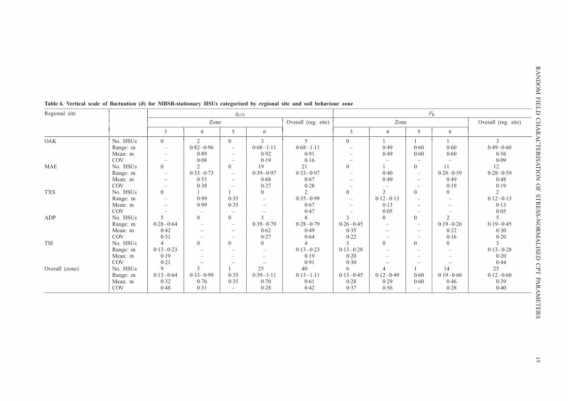
Table 4. Vertical scale of fluctuation (�) for MBSR-stationary HSUs categorised by regional site and soil behaviour zone

Regional site qc1N FR

Zone Overall (reg. site) Zone Overall (reg. site)

3 4 5 6 3 4 5 6

OAK No. HSUs 0 2 0 3 5 0 1 1 1 3Range: m – 0.82–0.96 – 0.68–1.11 0.68–1.11 – 0.49 0.60 0.60 0.49–0.60Mean: m – 0.89 – 0.92 0.91 – 0.49 0.60 0.60 0.56COV – 0.08 – 0.19 0.16 – – – – 0.09

MAE No. HSUs 0 2 0 19 21 0 1 0 11 12Range: m – 0.33–0.73 – 0.39–0.97 0.33–0.97 – 0.40 – 0.28–0.59 0.28–0.59Mean: m – 0.53 – 0.68 0.67 – 0.40 – 0.49 0.48COV – 0.38 – 0.27 0.28 – – – 0.19 0.19

TXS No. HSUs 0 1 1 0 2 0 2 0 0 2Range: m – 0.99 0.35 – 0.35–0.99 – 0.12–0.13 – – 0.12–0.13Mean: m – 0.99 0.35 – 0.67 – 0.13 – – 0.13COV – – – – 0.47 – 0.05 – – 0.05

ADP No. HSUs 5 0 0 3 8 3 0 0 2 5Range: m 0.28–0.64 – – 0.39–0.79 0.28–0.79 0.26–0.45 – – 0.19–0.26 0.19–0.45Mean: m 0.42 – – 0.62 0.49 0.35 – – 0.22 0.30COV 0.31 – – 0.27 0.64 0.22 – – 0.16 0.20

TSI No. HSUs 4 0 0 0 4 3 0 0 0 3Range: m 0.13–0.23 – – – 0.13–0.23 0.13–0.28 – – – 0.13–0.28Mean: m 0.19 – – – 0.19 0.20 – – – 0.20COV 0.21 – – – 0.91 0.30 – – – 0.44

Overall (zone) No. HSUs 9 5 1 25 40 6 4 1 14 25Range: m 0.13–0.64 0.33–0.99 0.35 0.39–1.11 0.13–1.11 0.13–0.45 0.12–0.49 0.60 0.19–0.60 0.12–0.60Mean: m 0.32 0.76 0.35 0.70 0.61 0.28 0.29 0.60 0.46 0.39COV 0.48 0.31 – 0.28 0.42 0.37 0.56 – 0.28 0.40

RA

ND

OM

FIE

LD

CH

AR

AC

TE

RIS

AT

ION

OF

ST

RE

SS

-NO

RM

AL

ISE

DC

PT

PAR

AM

ET

ER

S1

5

the null hypothesis of weak stationarity for spatially corre-lated data of varying record lengths in a manner that isconsistent with the underlying autocorrelation model (ACM).Linear detrending based on regression is applied to producezero-mean fluctuations. Because the choice of ACM is veryimportant in the modified Bartlett test, this paper imposesstringent criteria on the manner in which the ACM is fittedto the sample autocorrelation function: only values largerthan Bartlett limits are fitted, and the coefficient of determi-nation of the fit must exceed 0.9. At the end of this rigorousprocedure, only 40 qc1N profiles and 25 FR profiles weredeemed sufficiently homogeneous from both physical andstatistical considerations to be analysed further as a weaklystationary random field. The majority of the acceptableprofiles were found in sandy soils, although some profiles inoverconsolidated fine-grained soils were available as well.

A random field may be described concisely in the second-moment sense by the scale of fluctuation and the coefficientof variation. A careful study of these important statistics waspresented. First, it was verified that the statistics were notbiased by the number of CPT measurement points withineach HSU, the CPT measurement interval, and the best-fitautocorrelation model (ACM). Second, the statistics com-puted from qc1N and FR were studied separately by plotting

them against mean qc1N and mean FR respectively. Theeffect of soil type was then interpreted using the Robertson(1990) chart, which considers mean qc1N and mean FR

jointly. Finally, if sufficient data are available, site-specificeffects not explainable by mean qc1N, mean FR, and soil typewere highlighted.

Generally, it was observed that qc1N is more stronglyspatially correlated than FR, with scales of fluctuation esti-mated in the range 0.1–1.2 m and 0.1–0.6 m respectively.This general trend is also discernible at the site level. Theprobable physical basis for this observation is that qc1N isinfluenced by a volume of soil around the cone tip that islarger than the sampling interval. Hence a few continuousvalues of qc1N are basically affected by almost the samevolume of soil as the cone penetrates. In contrast, FR isaffected only by the adjacent soil. It was also observed thatthe vertical scale of fluctuation of qc1N increases with in-creasing qc1N, whereas the vertical scale of fluctuation of FR

decreases with increasing FR. Because qc1N increases fromzone 3 to 6 and FR decreases from zone 3 to 6, theseobservations appear to indicate a consistent soil-type effect.A consistent soil-type effect was observed for the coefficientof variation of inherent variability as well. In general,cohesionless soils produced more variable normalised CPT

"8

,"8

"35

"@8

��

��

��

�

� � �

�!

� �� 3�� !

�!

"8

,"8

"35

"@8

��

��

��

�

� �

�!

�� 3�� !��

�!

Fig. 10. Coefficient of variation of inherent variability against mean value in HSU for MBSR-stationary HSUs, categorisedby best-fit ACM: (a) qc1N profiles; (b) FR profiles

*45

346

78"

49:

��

��

��

�

� � �

�!

� �� 3�� !

�!

*45

346

78"

49:

��

��

��

�

� �

�!

�� 3�� !��

�!

7"; 7";

Fig. 11. Coefficient of variation of inherent variability against mean value in HSU for MBSR-stationary HSUs, categorisedby regional site: (a) qc1N profiles; (b) FR profiles


Table 5. Coefficient of variation of inherent variability (�) for MBSR-stationary HSUs categorised by best-fit ACM and soil behaviour zone

ACM qc1N FR

Zone Overall(ACM)

Zone Overall(ACM)

3 4 5 6 3 4 5 6

SNX No. HSUs 1 1 0 2 4 3 1 0 2 6Range 0.04 0.18 – 0.20–0.25 0.04–0.25 0.10–0.21 0.18 – 0.17–0.17 0.10–0.21Mean 0.04 0.18 – 0.23 0.17 0.15 0.18 – 0.17 0.16COV – – – 0.11 0.47 0.29 – – 0 0.21

CSX No. HSUs 4 0 0 4 8 1 3 1 3 8Range 0.02–0.17 – – 0.17–0.24 0.02–0.24 0.14 0.13–0.17 0.38 0.12–0.59 0.12–0.59Mean 0.08 – – 0.20 0.14 0.14 0.15 0.38 0.34 0.25COV 0.80 – – 0.13 0.55 – 0.11 – 0.57 0.63

SMK No. HSUs 3 3 1 9 16 2 0 0 9 11Range 0.05–0.21 0.19–0.28 0.24 0.18–0.30 0.05–0.30 0.18–0.20 – – 0.10–0.48 0.10–0.48Mean 0.13 0.22 0.24 0.24 0.22 0.19 – – 0.22 0.22COV 0.49 0.18 – 0.16 0.27 0.05 – – 0.47 0.44

SQX No. HSUs 1 1 0 10 12 0 0 0 0 0Range 0.14 0.33 – 0.18–0.38 0.14–0.38 – – – – –Mean 0.14 0.33 – 0.24 0.27 – – – – –COV – – – 0.27 0.29 – – – – –

Overall (zone) No. HSUs 9 5 1 25 40 6 4 1 14 25Range 0.02–0.21 0.18–0.33 0.24 0.17–0.38 0.02–0.38 0.10–0.21 0.13–0.18 0.38 0.10–0.59 0.10–0.59Mean 0.10 0.24 0.24 0.23 0.20 0.16 0.16 0.38 0.24 0.21COV 0.66 0.25 – 0.22 0.38 0.23 0.12 – 0.56 0.53

RA

ND

OM

FIE

LD

CH

AR

AC

TE

RIS

AT

ION

OF

ST

RE

SS

-NO

RM

AL

ISE

DC

PT

PAR

AM

ET

ER

S1

7

Table 6. Coefficient of variation of inherent variability (�) for MBSR-stationary HSUs categorised by regional site and soil behaviour zone

Regional site qc1N FR

Zones Overall (reg. site) Zones Overall (reg. site)

3 4 5 6 3 4 5 6

OAK No. HSUs 0 2 0 3 5 0 1 1 1 3Range – 0.18–0.20 – 0.18–0.25 0.18–0.25 – 0.17 0.38 0.22 0.17–0.38Mean – 0.19 – 0.21 0.20 – 0.17 0.38 0.22 0.26COV – 0.05 – 0.14 0.13 – – – – 0.35

MAE No. HSUs 0 2 0 19 21 0 1 0 11 12Range – 0.19–0.28 – 0.17–0.38 0.17–0.38 – 0.18 – 0.10–0.31 0.10–0.31Mean – 0.24 – 0.24 0.24 – 0.18 – 0.19 0.19COV – 0.19 – 0.23 0.23 – – – 0.32 0.31

TXS No. HSUs 0 1 1 0 2 0 2 0 0 2Range – 0.33 0.24 – 0.24–0.33 – 0.13–0.15 – – 0.13–0.15Mean – 0.33 0.24 – 0.29 – 0.14 – – 0.14COV – – – – 0.16 – 0.07 – – 0.07

ADP No. HSUs 5 0 0 3 8 3 0 0 2 5Range 0.11–0.21 – – 0.20–0.24 0.11–0.24 0.14–0.21 – – 0.48–0.59 0.14–0.59Mean 0.15 – – 0.22 0.18 0.18 – – 0.54 0.32COV 0.22 – – 0.08 0.25 0.17 – – 0.10 0.03

TSI No. HSUs 4 0 0 0 4 3 0 0 0 3Range 0.02–0.05 – – 5 0.02–0.05 0.10–0.18 – – – 0.10–0.18Mean 0.03 – – – 0.03 0.14 – – – 0.14COV 0.40 – – – 1.28 1.24 – – – 1.24

Overall (zone) No. HSUs 9 5 1 25 40 6 4 1 14 25Range 0.02–0.21 0.18–0.33 0.24 0.17–0.38 0.02–0.38 0.10–0.21 0.13–0.18 0.38 0.10–0.59 0.10–0.59Mean 0.10 0.24 0.24 0.23 0.20 0.16 0.16 0.38 0.24 0.21COV 0.66 0.25 – 0.22 0.38 0.23 0.12 – 0.56 0.53

18

UZ

IEL

LI,

VA

NN

UC

CH

IA

ND

PH

OO

N

measurements than cohesive soils. This observation is inagreement with previous studies on non-normalised CPTmeasurements.

Comparison with literature data indicates that the maineffects of normalisation are possibly a decrease in the scaleof fluctuation for cone tip resistance and definitely a reduc-tion in the coefficient of variation. These observations arecompatible with the fact that normalisation tends to mini-mise systematic physical in-situ effects that may introducesubtle trends and hence longer correlation lengths and largercoefficients of variation in the data. However, it is possiblethat part of the decrease may be attributed to the degree ofphysical homogeneity in HSU profiles, which was strictlycontrolled in this study.

REFERENCESAgterberg, F. B. (1970). Autocorrelation functions in geology.

Proceedings of a colloquium on geostatistics, University ofKansas, Lawrence, pp. 113–141.

Akkaya, A. D. & Vanmarcke, E. H. (2003). Estimation of spatialcorrelation of soil parameters based on data from the TexasA&M University NGES. In Probabilistic site characterization atthe National Geotechnical Experimentation Sites (eds G. A.Fenton and E. H. Vanmarcke), pp. 29–40. ASCE GeotechnicalSpecial Publication No. 121, pp. 29–40.

Alonso, E. E. & Krizek, R. J. (1975). Stochastic formulation of soilproperties. Proc. 2nd Int. Conf. on Applications of Statistics &Probability in Soil and Structural Engineering, Aachen 2, pp.9–32.

Baecher, G. B. (1986). Geotechnical error analysis. Transp. Res.Rec., No. 1105, 23–31.

Baecher, G. B. (1999). Discussion on inaccuracies associated withestimating random measurement errors. J. Geotech. Engng 125,No. 1, 79–81.

Baecher, G. B. & Christian, J. T. (2003). Reliability and statistics ingeotechnical engineering. New York: John Wiley & Sons.

Box, G. E. P. & Jenkins, G. M. (1970). Time series analysis:Forecasting and control. San Francisco: Holden Day.

Brockwell, P. J. & Davis, R. A. (1991). Time series: Theory andmethods, 2nd edn. New York: Springer-Verlag.

Cafaro, F. & Cherubini, C. (2002). Large sample spacing in evalua-tion of vertical strength variability of clayey soil. J. Geotech.Geoenviron. Engng 128, No. 7, 558–568.

Campanella, R. G., Wickremesinghe, D. S. & Robertson, P. K.(1987). Statistical treatment of cone penetrometer test data.Proc. 5th Int. Conf. on Applications of Statistics and Probabilityin Soil and Structural Engineering, Vancouver 2, 1011–1019.

DeGroot, D. J. & Baecher, G. B. (1993). Estimating autocovariancesof in-situ soil properties. J. Geotech. Engng 119, No. 1, 147–166.

DeJong, J. T. & Frost, J. D. (2002). A multi-friction sleeve attach-ment for the cone penetrometer. ASTM J. Geotech. Test. 25, No.2, 111–127.

Elkateb, T., Chalaturnyk, R. & Robertson, P. K. (2003a). Anoverview of soil heterogeneity: quantification and implicationson geotechnical field problems. Can. Geotech. J. 40, 1–15.

Elkateb, T., Chalaturnyk, R. & Robertson, P. K. (2003b). Simplifiedgeostatistical analysis of earthquake-induced ground response atthe Wildlife Site, California, USA. Can. Geotech. J. 40, 16–35.

Fenton, G. (1999). Random field modeling of CPT data. J. Geotech.Geoenviron. Engng 125, No. 6, 486–498.

Green, R. & Becker, D. (2001). National report on limit statedesign in geotechnical engineering: Canada. Geotech. News 19,No. 3, 47–55.

Harr, M. E. (1987). Reliability-based design in civil engineering.New York: McGraw Hill.

Jaksa, M. B. (1995). The influence of spatial variability on thegeotechnical design properties of a stiff, overconsolidated clay.PhD Dissertation, University of Adelaide.

Jaksa, M. B., Brooker, P. I. & Kaggwa, W. S. (1997). Inaccuraciesassociated with estimating random measurement errors. J. Geo-tech. Geoenviron. Engng 123, No. 5, 393–401.

Kulhawy, F. H. & Phoon, K. K. (2002). Observations on geotechni-

cal reliability-based design development in North America.Proceedings of the international workshop on foundation designcodes and soil investigation in view of international harmoniza-tion and performance based design, Hayama, pp. 31–48.

Kulhawy, F. H. & Trautmann, C. H. (1996). Estimation of in-situtest uncertainty. In Uncertainty in the geologic environment:From theory to practice (eds C. D. Shackleford, P. P. Nelson andM. J. S. Roth), pp. 269–286. ASCE Geotechnical SpecialPublication No. 58.

Kulhawy, F. H., Birgisson, B. & Grigoriu, M. D. (1992). Reliability-based foundation design for transmission line structures: Trans-formation models for in-situ tests, Report EL-5507(4). Palo Alto,CA: Electric Power Research Institute.

Lacasse, S. & Nadim, F. (1996). Uncertainties in characterizing soilproperties. In Uncertainty in the geologic environment: Fromtheory to practice (eds C. D. Shackleford, P. P. Nelson and M. J.S. Roth), pp. 49–75. ASCE Geotechnical Special PublicationNo. 58.

Lunne, T., Robertson, P. K. & Powell, J. J. M. (1997). Conepenetration testing in geotechnical practice. London: E&FNSpon.

Nadim, F. (1986). Probabilistic site description strategy, Report51411–4. Oslo: Norwegian Geotechnical Institute.

Orchant, C. J., Kulhawy, F. H. & Trautmann, C. H. (1988).Reliability-based foundation design for transmission line struc-tures: Critical evaluation of in-situ test methods, Report EL-5507(2). Palo Alto, CA: Electric Power Research Institute.

Phoon, K. K. & Kulhawy, F. H. (1996). On quantifying inherentsoil variability. In Uncertainty in the geologic environment:From theory to practice (eds C. D. Shackleford, P. P. Nelson andM. J. S. Roth), pp. 326–340. ASCE Geotechnical SpecialPublication No. 58.

Phoon, K. K. & Kulhawy, F. H. (1999a). Characterization ofgeotechnical variability. Can. Geotech. J. 36, No. 4, 612–624.

Phoon, K. K. & Kulhawy, F. H. (1999b). Evaluation of geotechnicalproperty variability. Can. Geotech. J. 36, No. 4, 625–639.

Phoon, K. K., Kulhawy, F. H. & Grigoriu, M. D. (1995). Reliabil-ity-based design of foundations for transmission line structures,Report T-105000. Palo Alto, CA: Electric Power ResearchInstitute.

Phoon, K. K., Quek, S. T. & An, P. (2003). Identification ofstatistically homogeneous soil layers using modified Bartlettstatistics. J. Geotech. Geoenviron. Engng 129, No. 7, 649–659.

Popescu, R., Prevost, J. H. & Deodatis, G. (1998). Characteristicpercentile of soil strength for dynamic analysis. Proc. 3rd Conf.on Geotechnical Earthquake Engineering and Soil Dynamics,Seattle 2, 1461–1471.

Priestley, M. B. (1981). Spectral analysis and time series. Orlando,FL: Academic Press.

Reyna, F. & Chameau, J. L. (1991). Statistical evaluation of CPT &DMT measurements at the Heber Road Site. GeotechnicalEngineering Congress (eds F. G. McLean, D. A. Campbell & D.W. Harris), pp. 14–25. New York: American Society of CivilEngineers.

Robertson, P. K. (1990). Soil classification using the cone penetra-tion test. Can. Geotech. J. 27, No. 1, 151–158.

Robertson, P. K. & Wride, C. E. (1998). Evaluating cyclic liquefac-tion potential using the cone penetration test. Can. Geotech. J.35, No. 3, 442–459.

Spry, M. J., Kulhawy, F. H. & Grigoriu, M. D. (1988). Reliability-based foundation design for transmission line structures: Geo-technical site characterization strategy, Report EL-5507(1). PaloAlto, CA: Electric Power Research Institute.

Tang, W. H. (1979). Probabilistic evaluation of penetration resis-tances. J. Geotech. Engng Div., ASCE 105, No. 10, 1173–1191.

Teh, C. I. & Houlsby, G. T. (1991). An analytical study of the conepenetration test in clay. Geotechnique 41, No. 1, 17–34.

Uzielli, M. (2004). Variability of stress-normalized CPT parametersand application to seismic liquefaction initiation analysis. PhDdissertation, University of Florence.

Uzielli, M., Vannucchi, G. & Phoon, K. K. (2004). Assessment ofweak stationarity using normalized cone tip resistance. Proceed-ings of the ASCE joint specialty conference on probabilisticmechanics and structural reliability, Albuquerque (CD-ROM).

Vanmarcke, E. H. (1983). Random fields: Analysis and synthesis.Cambridge, MA: MIT Press.


Watson, G. S. (1967). Linear least squares regression. Annals ofMathematical Statistics 38, 1679–1699

Wickremesinghe, D. S. (1989). Statistical characterization of soilprofiles using in situ tests. PhD Dissertation, University ofBritish Columbia.

Withiam, J. L. (2003). Implementation of the AASHTO LRFDBridge Design Specifications for Substructure Design. Proceed-ings of the international workshop on limit state design ingeotechnical engineering practice, Massachusetts Institute ofTechnology, Cambridge (CD-ROM).

Wroth, C. P. (1984). The interpretation of in situ soil test. Geotech-nique 34, No. 4, 449–489.

Wu, T. H., Lee, I.-M., Potter, J. C. & Kjekstad, O. (1987).Uncertainties in evaluation of strength of marine sand. J.Geotech. Engng 113, No. 7, 719–738.

Youd, T. L., Idriss, I. M., Andrus, R. D., Arango, I., Castro, G.,Christian, J. T., Dobry, R., Finn, W. D. L., Harder, L. F. Jr,Hynes, M. E., Ishihara, K., Koester, J. P., Liao, S. S. C.,Marcuson, W. F. III, Martin, G. R., Mitchell, J. K., Moriwaki,Y., Power, M. S., Robertson, P. K., Seed, R. B. & Stokoe, K. H.II. (2001). Liquefaction resistance of soils: Summary reportfrom the 1996 NCEER and 1998 NCEER/NSF Workshops onEvaluation of Liquefaction Resistance of Soils. J. Geotech.Geoenviron. Engng 127, No. 10, 817–833.


random field characterisation of stress-normalised cone penetration testing parameters

Documents