rand - defense technical information center · a rand note n-2283/3-af aircraft airframe cost...

A RAND NOTE

C" Aircraft Airframe Cost Estimating Relationships:

I Bombers and Transports

NR. W. Hess, H. P. Romanoff

D December 1987

DTICTELECTE uh

41988

DLSTRM~U'MON ;'7'-jl A

RAND 88 10 24 005

RAND

The research reported here was sponsored by the United States Air Forceunder Contract F49620-86-C-OOO& Further information may be obtained fromthe Long Range Planning and Doctrine Division, Directorate of Plans, HqUSAF.

The RAND Publication Series: The Report is the principal publication documen-ting and transmitting RAND's major research findings and final research results.The RAND Note reports other outputs of sponsored research for general distri-bution. Publications of The RAND Corporation do not necessarily reflect theopinions or policies of the sponsors of RAND research.

Published by The RAND Corporation1700 Main Street, P.O. Box 2138, Santa Monica, CA 90406-2138

UNCLASSIFIED

SECURITY CLASSIFICATION OF THIS PAGF '*%we -*IA Entered)

REPORT DOCUMENTATION PAGE READ INSTRUCTIONSBEFORE COMPLETING FORM

1 REPORT NUMBER 2. GOVT ACCESSION NO. 3. RECIPIENT'S CATALOG NUMBERN-2283/3-AF

4. TITLE (and Subtitle) S. TYPE OF REPORT & PERIOD COVERED

Aircraft Airframe Cost Estimating Relationships: Interim

Bombers and Transports 6. PERFORMING ORG. REPORT NUMBER

7. AUTWOR(e) 8. CONTRACT OR GRANT NUMBER(e)

R. W. Hess, H. P. Romanoff F49620-86-C-0008

9. PERFORMING ORGANIZATION NAME AND AODRESS 10. PROGRAM ELEMENT. PROJECT. TASK

AREA & WORK UNIT NUMBERSThe RAND Corporation1700 Main StreetSanta Monica, CA 90406

I I. CONTROLLING OFFICE NAME AND AOORESS 12. REPORT DATEDirectorate of Plans December 1987Office, DCS/Plans and Operations 13. NUMBEROF PAGESHq, USAF, Washington, DC 20330 51

It. MONITORING ACENCY NAME & ADORESSII diffeent Irue CONSIrollin5 Office) IS. SECURITY CLASS. (of tis report)

Unclassified

IS. OECLASSIFICATION/DOWNGRAOINGSC4EDULE 0

I6. DISTRIBUTION STATEMENT (of this Report)

Approved for Public Release; Distribution Unlimited

77. DISTRIBUTION STATEMENT (of the abetract entered In Block 20. it different Ifrm Report)

No Restrictions

IS. SUPPLEMENTARY NOTES

19 KEY WORDS (Conitnue on reerse aide , neceeeery and Identify by block number)

Airframes, Bomber Aircraft.,Cost Estimates, Transport Aircraft,Procurement, Military Aircraft..Equations I

20 ABSTRACT (Continue on Peeree eide It neceeery and Idemtify by block number)

See reverse side

DO jAN",, 1473 UNCLASSIFTED

SECURITY CLASSIFICATION OF THIS PAGE ,When Dee Entered)

w w w w • V V V V _ S S 0

UNCLASSIFIED

$1CURIITY CLA"IIPICATION Of THIS PAGlthmM Data 9WOMe) ,

This Note is part of a series of Notes thatderive a set of equations suitable forestimating the acquisition costs of varioustypes of aircraft airframes in the absenceof detailed design and manufacturinginformation. A single set of equat:ions wasselected as being the most representativeand applicable to the widest range ofestimating situations. For bombers andtransports, no single acceptable estimatingrelationship could be identified.

Estimates for these aircraft shou]d bedeveloped by analogy or by using theequation set developed for all missiontypes. K> -

0

0* 0

* 0

UNCLASSIFTED

SECURITY CLASSIFICATION Of THIS PAGE(mWh. Di Ene,ed)

III • • 3 • • w w w w

A RAND NOTE N-2283/3-AF

Aircraft Airframe Cost Estimating Relationships:

Bombers and Transports

R. W. Hess, H. P. Romanoff

December 1987

Prepared for \ 1

The United States Air Force

RAND APPROVED FOR PUBLIC RELEASE; DISTRIBUTIONUNITE

.. - * *** * . I*

- iii -

PREFACE

This Note describes an attempt to develop a set of equations

suitable for estimating the acquisition costs of bomber/transport

airframes in the absence of detailed design and manufacturing

information. In broad form, this research represents an extension of

the results published in J. P. Large et al., Parametric Equations for

Estimating Aircraft Airframe Costs, The RAND Corporation, R-1693-I-PA&E,

February 1976, and used in the RAND aircraft cost model, DAPCA: H. E.

Boren, Jr., A Computer Model for Estimating Development and Procurement

Costs of Aircraft (DAPCA-III), The RAND Corporation, R-1854-PR, March

1976.

The present effort was undertaken in the context of a larger

overall study whose objectives included: (a) an analysis of the utility

of dividing the full estimating sample into subsamples representing

major differences in aircraft type (attack, fighter, and

bomber/transport); and (b) an examination of Lhe explanatory power of

variables describing program structure and airframe construction

techniques. Additionally, for the fighter subsample only, the study

investigated the possible benefits of incorporating an objective

technology measure into the equations. A detailed description of the

overall study including the research approach, evaluation criteria, and

database may be found in R. W. Hess and H. P. Romanoff, Aircraft

Airframe Cost Estimating Relationships: Study Approach and Conclusions,

The RAND Corporation, R-3255-AF, December 1987.

To address the issue of sample homogeneity, each of the subsamples,

as well as the full sample, had to be investigated in detail with the

ultimate goal of developing a representative set of cost estimating

relationships (CERs) for each. The purpose of this Note is, therefore,

to document the analysis of the bomber/transport subsample. Study

results concerning the full estimating sample as well as the other

subsamples are available in a series of companion Notes:

01

- iv -

Aircraft Airframe Cost Estimating Relationships: All Mission Types,N-2283/1-AF, December 1987.

Aircraft Airframe Cost Estimating Relationships: Fighters,N-2283/2-AF, December 1987.

Aircraft Airframe Cost Estimating Relationships: Attack Aircraft,N-2283/4-AF, December 1987.

This research was undertaken as part of the Project AIR FORCE study

entitled "Cost Analysis Methods for Air Force Systems," which has since

been superseded by "Air Force Resource and Financial Management Issues

for the 1980s" in the Resource Management Program.

While this report was in preparation, Lieutenant Colonel H. P.

Romanoff, USAF, was on duty in the System Sciences Department of The

RAND Corporation. At present, he is with the Directorate of Advanced

Programs in the Office of the Assistant Secretary of the Air Force for

Acquisition.

0

___ _ ____ _ _ *

-v-

SUMMARY

This Note documents an attempt to derive a set of equations

suitable for estimating the acquisition costs of bomber/transport

aircraft. The estimating sample consists of eight bomber/transport

aircraft with first flight dates ranging from 1954 to 1968. The

aircraft technical data were for the most part obtained from either

original engineering documents such as manufacturer's performance

substantiation reports or from official Air Force and Navy documents.

The cost data were obtained from the airframe manufacturers either

directly from their records or indirectly through standard Department of

Defense reports such as the Contractor Cost Data Reporting System.

The key result of this effort is that we were unable to identify a

single acceptable estimating relationship for any of the individual cost

elements or for the total program cost element. This discouraging

result is not too surprising, however, since the bomber/transport sample

is very small and not especially homogeneous. Estimates for proposed

bomber/transport aircraft should be developed on the basis of analogy

(using the data provided in this Note) or by using the equation set

developed for all mission types (N-2283/1-AF).

0.i

- vii -

CONTENTS

PREFACE . .......................................................... iii

SUMMARY ... .......................................................... v

F IGURES .. ........................................................... ix

TABLES..............................................................xi

MNEMONICS ............................................................ xiii

EVALUATION CRITERIA NOTATION .. .................................... xv

SectionI. INTRODUCTION .............................................. I

II. DATABASE AND ANALYTICAL APPROACH ... .......................... 3Estimating Sample ... ....................................... 3Dependent Variables ..................................... 4Potential Explanatory Variables ......................... 5Approach ... ................................................ 8Evaluation Criteria .. .................................... 11

III. INITIAL OBSERVATIONS ...................................... 17Influential Observations ................................ 17rerformance variables .. ................................... 19Construction/Program Variables .......................... 19

IV. ENGINEERING .. .............................................. 20

V. TOOLTNG .. .................................................. .23

VI. MANUFACTURING LABOR .. ...................................... 26

VII. MANUFACTURING MATERIAL .. ................................... 29

VIII. DEVELOPMENT SUPPORT .. ...................................... 32

IX. FLIGHT TEST .. .............................................. 36

X. QUALITY CONTROL .. .......................................... 39

XI. TOTAL PROGRAM COST .. ....................................... 41

XII. CONCLUSIONS ............................................... 44Cost-Quantity Slopes .................................... 44Fully Burdened Labor Rates .............................. 45

Appendix: CORRELATTON MATRTXS .................... ........... 47

REFERENCES .. ....................................................... 51

I-

-ix-

FIGURES

1. Number of First Flight Events as a Function of the Yearof First Flight ........................................... 16

2. Effect of B/RB-66 and C-5 ................................. 19

3. Engineering Hours per Pound as a Function of AirframeUnit Weight ............................................... 21

4. Tooling Hours per Pound as a Function of Airframe UnitW eight .................................................... 24

5. Manufacturing Labor Hours per Pound as a Function ofAirframe Unit Weight ...................................... 27

6. Manufacturing Material Cost per Pound as a Function ofAirframe Unit Weight ...................................... 30

7. Development Support Cost per Pound as a Function ofAirframe Unit Weight ...................................... 33

8. Flight Test Cost per Test Aircraft as a Function of theQuantity of Flight Test Aircraft .......................... 37

9. Quality Control Hours per Pound as a Function ofAirframe Unit Weight ...................................... 40

10. Total Program Cost per Pound as a Function of AirframeUnit Weight ............................................... 42

ix

- xi -

TABLES

1. Percentage Breakdown of Bomber/Transport AirframeProgram Costs ............................................. 4

2. Bomber/Transport Aircraft Characteristics ................. 6

3. A Priori Notions Regarding Effect of ExplanatoryVariable Increase on Cost Element .......................... 9

4. Comparison of Full Bomber/Transport Sample and SampleExcluding B-58 ............................................. 18

5. Engineering Hour Estimating Relationships ................. 22

6. Tooling Hour Estimating Relationships ..................... 25

7. Manufacturing Labor Hour Estimating Relationships ......... 28

8. Manufacturing Material Cost Estimating Relationships ...... 31

9. Development Support Cost Estimating Relationships ......... 34

10. Development Support Cost as a Percentage of Unit 1Engineering Cost ........................................... 35

11. Flight Test Cost Estimating Relationships ................. 38

12. Total Program Cost Estimating Relationships ................ 43

13. Cumulative Total Cost Quantity Slopes ..................... 45

A.l. Correlation Matrix: Cost Variables with PotentialExplanatory Variables ..................................... 49

A.2. Correlation Matrix for Identification of PairwiseCollinearity ... ............................................. 50

LI I

- xiii -

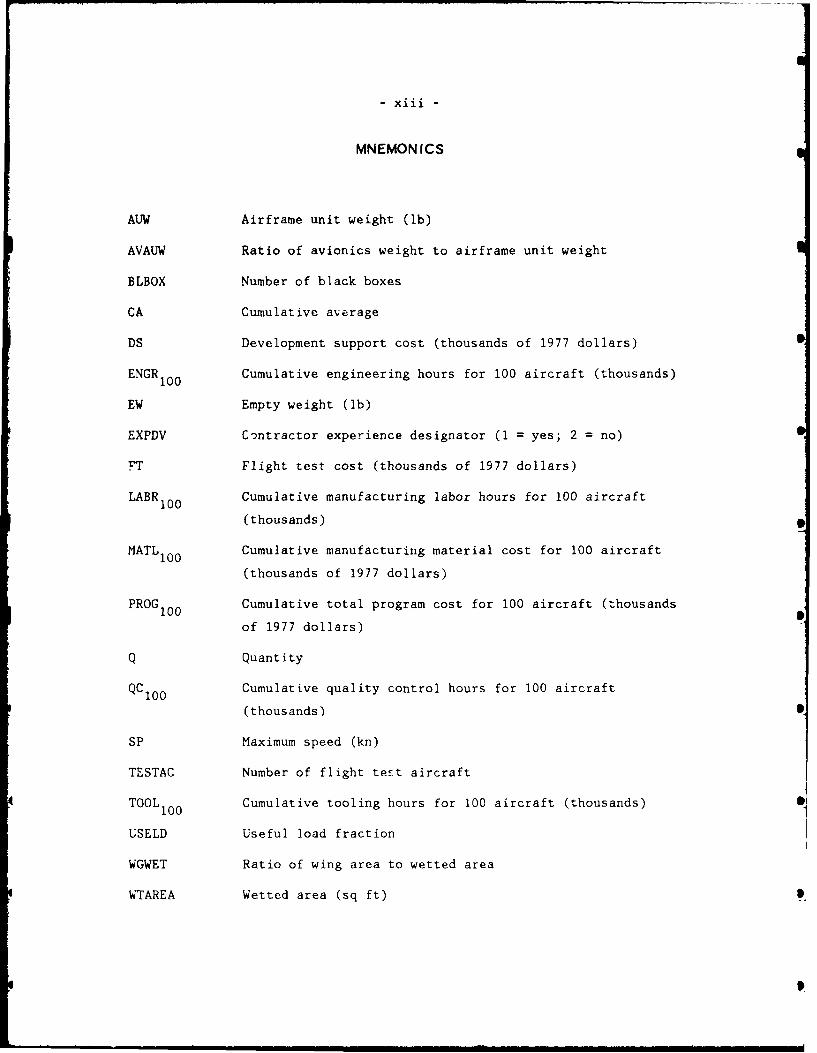
MNEMONICS

AUW Airframe unit weight (lb)

AVAUW Ratio of avionics weight to airframe unit weight

BLBOX Number of black boxes

CA Cumulative average

DS Development support cost (thousands of 1977 dollars)

ENGR 10 Cumulative engineering hours for 100 aircraft (thousands)

EW Empty weight (lb)

EXPDV Contractor experience designator (1 = yes; 2 = no)

FT Flight test cost (thousands of 1977 dollars)

LABRI00 Cumulative manufacturing labor hours for 100 aircraft

(thousands)

MATL100 Cumulative manufacturing material cost for 100 aircraft

(thousands of 1977 dollars)

PROG100 Cumulative total program cost for 100 aircraft (thousands

of 1977 dollars)

Q Quantity

QC1o O Cumulative quality control hours for 100 aircraft

(thousands)

SP Maximum speed (kn)

TESTAC Number of flight test aircraft

TOOL100 Cumulative tooling hours for 100 aircraft (thousands)

USELD Useful load fraction

WGWET Ratio of wing area to wetted area

WTAREA Wetted area (sq ft)

I -

- xv -

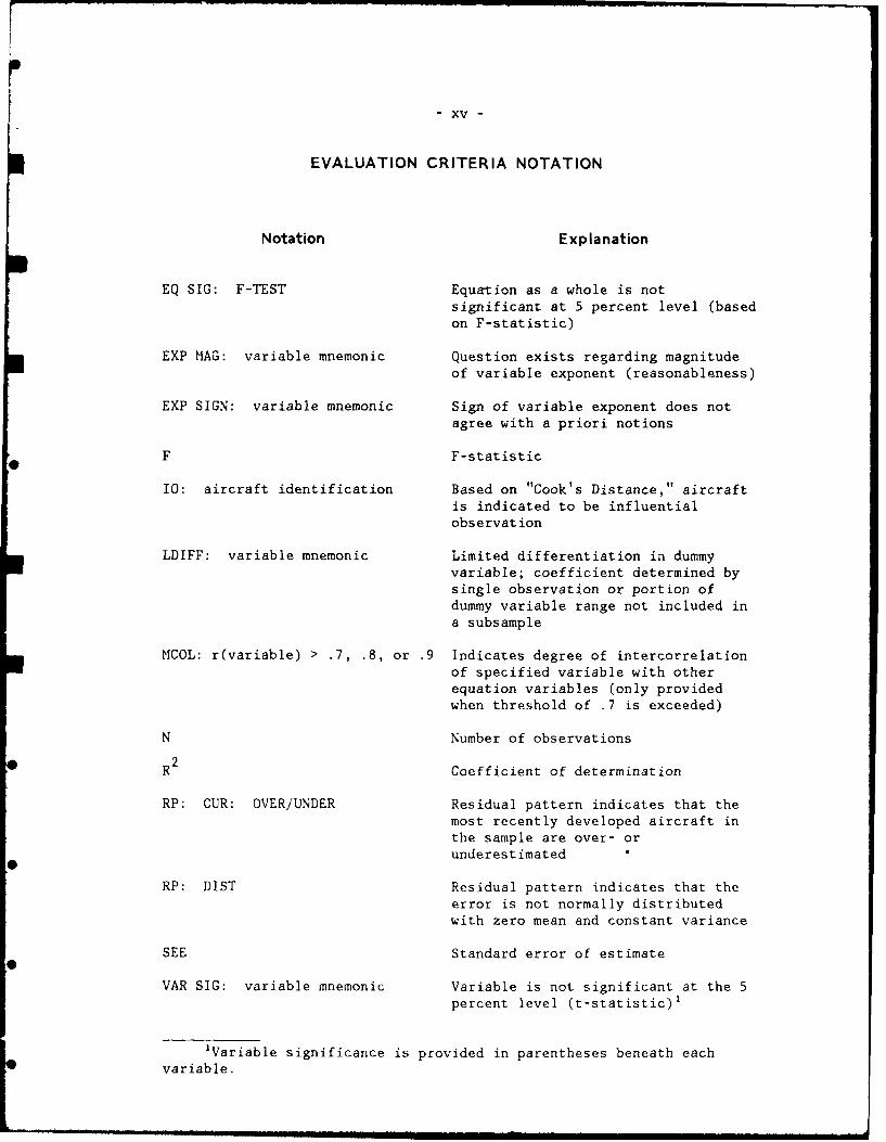
EVALUATION CRITERIA NOTATION

Notation Explanation

EQ SIG: F-TEST Equation as a whole is notsignificant at 5 percent level (basedon F-statistic)

EXP MAG: variable mnemonic Question exists regarding magnitudeof variable exponent (reasonableness)

EXP SIGN: variable mnemonic Sign of variable exponent does notagree with a priori notions

F F-statistic

10: aircraft identification Based on "Cook's Distance," aircraftis indicated to be influentialobservation

LDIFF: variable mnemonic Limited differentiation in dummyvariable; coefficient determined bysingle observation or portion ofdummy variable range not included ina subsample

MCOL: r(variable) > .7, .8, or .9 Indicates degree of intercorrelationof specified variable with otherequation variables (only providedwhen threshold of .7 is exceeded)

N Number of observations

R 2 Coefficient of determination

RP: CUR: OVER/UNDER Residual pattern indicates that themost recently developed aircraft inthe sample are over- orunderestimated

RP: DIST Residual pattern indicates that theerror is not normally distributedwith zero mean and constant variance

SEE Standard error of estimate

VAR SIG: variable mnemonic Variable is not significant at the 5percent level (t-statistic)l

'Variable significance is provided in parentheses beneath eachvariable.

1. INTRODUCTION

Parametric models for estimating aircraft airframe acquisition

costs have been used extensively in advanced planning studies and

contractor proposal validation. These models are designed to be used

when little is known about an aircraft design or when a readily applied

validity and consistency check of detailed cost estimates' is necessary.

They require inputs that: (a) will provide results that are relatively

accurate; (b) are logically related to cost; and (c) can easily be

projected prior to actual design and development. The intent is to

generate estimates that include the cost of program delays, engineering

changes, data requirements, and phenomena of all kinds that occur in r

normal aircraft program.

Since 1966, RAND has developed three parametric airframe cost

models.2 These models have been characterized by: (a) easily

obtainable size and performance inputs (weight and speed); (b) the

estimation of costs at the total airframe level; and (c) the utilization

of heterogeneous aircraft samples. They have normally been updated when

a sufficient number of additional aircraft data points has become

available to suggest possible changes in the equations. Such is the

case with the present effort: the A-10, F-15, F-16, F-18, F-101, and

S-3 have been added to the full estimating sample.'

In addition to the expansion of the database, we also examined:

(a) the utility of dividing the estimating sample into subsamples

representing major differences in aircraft type (attack, fighter,

bomber/transport); (b) the explanatory power of variables describing

'Examples of this latter application include the Independent CostAnalysis (ICA), prepared as part of the Defense Systems AcquisitionReview Council (DSARC) process, and government analyses of contractorcost proposals during source selections.

2See Refs. 1, 2, and 3.3Additionally, the F-86, F-89, and F3D, which were dropped from the

DAPCA-III estimating sample, were reintroduced.

-2-

program structure and airframe construction techniques; and (c) the

possible benefits of incorporating an objective technology measure into

the fighter sample equations. In order to address the issue of sample

homogeneity, each of the subsamples, as well as the full sample, had to

be investigated in detail with the ultimate goal of developing

representative sets 4 of cost estimating relationships (CERs) for each.

The purpose of this Note is, therefore, to document the analysis of the

bomber/transport subsample.

Section II provides brief descriptions of the database and

statistical analysis methods. Section III gives some general

indication, based on initial observations, of what can be expected in

subsequent sections. Sections IV through XI provide, by cost element,

data plots and each of the estimating relationships that meets our

initial screening criterion with respect to variable significance.

Section XII summarizes the main findings of the study. The appendix

contains correlation matrixes.

4A set encompasses the following cost elements: engineering,tooling, manufacturing labor, manufacturing material, developmentsupport, flight test, and quality control.

-3-

II. DATABASE AND ANALYTICAL APPROACH

A detailed description of the research approach, evaluation

criteria, and database for this study may be found in R-3255-AF.

However, in order that this Note may have a degree of self-sufficiency,

a synopsis of the database and analytical approach is presented prior to

the reporting of results.

ESTIMATING SAMPLE

The full bomber/transport estimating sample consists of the

following eight "new design" aircraft:'

First FlightModel Date'

B-52 1954B-58 1957

B/RB-66 1954C-5 1968C-130 1955C-133 1956

KC-135 1957C-141 1963

'The classification of an aircraft as new or derivative is not anentirely objective procedure. For example, although the B/RB-66 evolvedfrom the A-3, the B/RB-66 is classified as a new design in the database."During the course of B/RB-66 development, more than 400 alterationswere made, including a two-degree change in wing incidence, a reductionin the sweep angle of the inboard wing trailing edge to decreasethickness/chord ratio and minimize pitchup, and a completely newfuselage layout, and these changes, added to the specialized equipmentdemanded for the various B/RB-66 versions, resulted in a full-scaledevelopment project" (Ref. 4, p. 149).

2The first flight dates presented in this Note are intended toreflect the first flight date of the version of the aircraft that wasmost representative of the aircraft which was to become operational.Put another way, these dates are intended to reflect the first flightdate of the developmental aircraft and not earlier experimental orprototype aircraft.

.S

-4-

DEPENDENT VARIABLES

Costs have been dealt with at both the total program level3 and at

the major cost element level (engineering, tooling, manufacturing labor,

manufacturing material, development support, flight test, and quality

control).' The relative importance of the various cost elements is

shown in Table 1 for four alternative production quantities. Other

things being equal, the accuracy of the estimating relationship for

manufacturing labor is of greatest concern because of the relatively

large share of program cost represented by that cost element.

Table 1

PERCENTAGE BREAKDOWN OF BOMBER/TRANSPORTAIRFRAME PROGRAM COSTS

(8 aircraft average costs)

Quantity

Cost Element 25 50 100 200

Engineering 21 19 16 13Tooling 23 20 17 14Manufacturing labor 29 33 37 41Manufacturing material 11 15 19 23Development support 6 5 3 2Flight test 7 5 4 3Quality control 3 3 4 4

100 100 100 100

3Total program costs are "normalized" values and not the actualreported dollar amounts. They are normalized in the sense that thedollar amounts for engineering, tooling, manufacturing labor, andquality control have been determined by applying fully burdened,industry-average labor rates to the hours reported for each category.

4Cost element definitions are provided in Appendix A of R-3255-AF.

-5

Engineering, tooling, manufacturing labor, and quality control are

estimated in terms of manhours rather than dollars for two reasons: (a)

it avoids the need to make adjustments for annual price changes, and (b)

it permits comparison of real differences in labor requirements.1

Manufacturing material, development support, and flight test do not lend

themselves to this approach and were therefore estimated in terms of

dollars (in this case, constant 1977 dollars).

POTENTIAL EXPLANATORY VARIABLES

To be included among the characteristics that were considered for

inclusion in the CERs, a variable had to fulfill the following

requirements:

1. It had to be logically related to cost: that is, a rationale

had to be constructed that would explain why cost should be

influenced by the variable;

2. It had to be "readily available" in the early stages of

aircraft conceptualization; and

3. It had to have an available historical record.

During the formulation stage of this study, twenty aircraft

characteristics were identified as potential explanatory variables for

the bomber/transport sample CERs. Values for these characteristics,

which are grouped into four general categories--size, performance,

construction, and program, are provided in Table 2. Based on this

table, the following observations are made:

1. For any of the three size measures, the C-5 is approximately

twice as large as the next largest aircraft in the sample.

sThe major limitation of the manhour approach is that it does notaccount for differences in overhead rates. Consequently, differences insuch things as capital/labor ratios cannot be addressed.

• m i| i | • 0

CC

0 -

P-N 04 0 7 0%oO 0% -TCD N N 0%r %0 rI0 11 IN M0 -' N

00 UN~ C

NOO0~ N ; 0 *M

NOO 0% rl - I'JcliN

x 'o'

UeA 0rr. N * O M IN Ne4 U' , W- N

UI m-0%-- N0 * - Cjo

C n 11, 0 N-

I0 0*C 0E- \0%_-M

0 0r 00 N0 0~ N .U- N- l c ~ ~ 0 .

AL I ~ M% '0u r- 0--N -*

U-N n It' .i UM C

1- O'*r m ~ ~ r* % -0o~ m" z. . .

10. % ON* It' it' 0 -CNNCD0CJ 0co z, 0%\ M-* 0- .

zi z.

%D' % 0 0 - a, 0 NMMO -D NCN N

goF 0,N%0 N-it 0N0~00* MON -N CD >,N r- U'\ at NO 0N *It - N -- 41Cf

Ut' \0 00 tn -\O N .0 U.., m 0

Nr-0 1c; CL0 0

C 4

0- 10 = z;4l 0U 0 El -0I -. 41 Aj C ). WC) cv

4 0 0 4' 24 C-

CD M' 0 I' n ml 11- .c 'o- io 0) 4'- 0 C. )1

0).: 0 4) . 'n0% 1.- m D 0 0 - .L CC) 4 C1 '0V .' 0 . O C) - O.- M l 0

m 0: 0m L. -f 4) ).i' - 11... .)4' 0%i E C D - > 0 cv. Itccv =) a)- -N(DC) 4(D .- C) ~) C 0%I6 - U)M a.j MU.0 .- - a) 0- ,v- >%00 0 - 00) (I) Ev cc. 4 -0:; C C)2. -'~0 d)- ) mvACc 0

4' m 4-' 0V) a. CL - - 00 > Cm A-OX CC) -= m D - 0 (D -"0C : m0- I-O-0 vv'0 >,m .C L Inm 1fl ( L) -0 4 4Ll .- 4..1)0 00. 0 -041

L 0% -0U O ~ C-O C,-.c 0 0 z'> 4'.0 >.-E00 M- 0.Lc4' 0-00 S. IDc . It .4' 0m n. - f. C> (5 ) Q) 4J 0C m- (2 O0 1 0%cv U Em 3v z M)0.- c 0 CO D Ed)EG 0I- 0 C-0)L-

0E L U 0 4)mL )zm00m. ua .a)00

-7-

2. With regards to speed, all aircraft in the sample are subsonic

with the exception of the B-58 which is a Mach 2 aircraft.

Similarly, the B-58 rate of climb is over twice that of the

next fastest climbing aircraft in the sample.

3. The sample does not include any aircraft which are both

relatively large and relatively fast (such as the B-lA was to

have been--airframe unit weight of approximately 150,000 pounds

and speed of Mach 2--and the B-lB is to be--dash speed of about

Mach 1.2).

4. All of the sample aircraft have engines located in nacelles

under the wing and all are land-based. Thus, there is no

variation in these two variables and they will not be

considered further.

5. The B-58 flight test program utilized more than twice as many

aircraft as the next largest program.

There are, of course, differences between the aircraft which are

not accounted for in Table 2. Some of the differences relate to the way

an aircraft is constructed (materials, manufacturing technology), others

to the way the program is managed. In any case, it is difficult to find

an aircraft without at least one unique aspect. Therefore, the

following list is intended only to be indicative of the types of

differences which are difficult to account for in a generalized

parametric model.

1. The C-130 and C-133 are prop aircraft while all other sample

aircraft utilize turbojet or turbofan engines.

2. The KC-135 was designed and produced more or less concurrently

with the commercial 707 model.

3. The B/RB-66 was produced concurrently with the A-3, the

aircraft from which it evolved.

4. The B-58's utilization of honeycombed skin panels represented a

major state-of-the-art advance.

i - I - P " O

-8"

5. The C-5 program utilized the acquisition concepts of total

package procurement and concurrent development and production.

A priori notions regarding the effect an increase in the value of

an explanatory variable might have on each of the cost elements are

indicated in Table 3.

APPROACH

Potential explanatory variables have been divided into four general

categories--size, performance, construction, and program (see Table 3).

As discussed in R-3255-AF,' the "ideal" airframe cost estimating

relationship would incorporate one explanatory variable from each

category. Thus, there would be four independent variables per

estimating relationship. For the full estimating sample, which has 34

observations, the possible incorporation of four independent variables

presents no difficulties since there would still be 29 degrees of

freedom left with which to estimate the error term. Unfortunately, the

bomber/transport subsample has only eight observations and the

incorporation of four explanatory variables would leave only three

degrees of freedom with which to estimate the error term. Consequently,

the number of explanatory variables considered per equation for the

bomber/transport sample was tentatively limited to two.7

With respect to the specific combinations of variable categories

examined, it is our understanding that all airframe manufacturers use

some measure of size (usually weight) as their basic scaling dimension

in developing cost estimates (although other factors frequently do enter

in). Consequently, it did not seem unreasonable for a similar

6R. W. Hess and H. P. Romanoff, Aircraft Airframe Cost EstimatingRelationships: Study Approach and Conclusions, The RAND Corporation,R-3255-AF, December 1987, Sec. IV.

7We do not mean to suggest that this limit is an "absolute" maximumfor it is not (theoretically, one could use six explanatory variablesfor a bomber/transport equation and still have one degree of freedomleft). It simply reflects our judgment regarding an appropriate balancebetween sample size and the potential number of explanatory variables. 0

-0

0.J0 .+4 ..+ ++ +4+4 e~+' r

000L 4-j

Ox. 0 C.L~. 41 d

c W >W

m 0 mcz41au. ) 0 0

- 0

-Q) 4+ +4 + +++ + ~ . )O L-C 0

41. 4)(1

4. C.6 (.-fl 4.)

CD-'o0

(V. . -0) 4)01W 4)U~~ 10

0) L uj 0) -) a

0 0 aV) 0 Z.

z. >V 0)4) L4 - W .- -.

(~4 C~ C

0x -c 6(0%- N

L V C..

E- z .I .) . . . .

00

0~00

-cc t) LOol C.C) 0L0

0)CC.)C . 0 4)

0)~~0 L. *--c

10 -

assumption to be made on our part--a size variable must appear in all

equations (except for flight test in which case the number of test

aircraft is the mandatory variable). Therefore, with this additional

restriction, the specific variable combinations that were examined for

the bomber/transport sample are as follows:

SizeSize/PerformanceSize/ConstructionSize/Program

The first step in developing a representative set of CERs was to

identify all potentially useful estimating relationships for each costelement resulting from the variable combinations listed above. For this

first step, "potentially useful" included only those estimating

relationships in which all equation variables were significant at the 5

percent level. Since the number of variable combinations was relatively

small, all possible regressions were run and screened for variable

significance. Then, each equation satisfying this initial screening

criterion was scrutinized in accordance with a set of evaluation

criteria dealing with statistical quality and reasonableness of results

(these are described in a subsequent subsection).

The final step was the selection of the most suitable estimating

relationship for each cost element (i.e., the selection of a

representative set). Generally speaking, other things being equal, we

tried to select estimating relationships that satisfied the following

conditions:

" Each variable is significant at the 5 percent level

* Variables taken collectively are significant at the 5 percent

level

* Results are credible

* Unusual residual patterns are absent

0

i

- 1i -

If these conditions were satisfied by more than one equation, then the

objective was minimization of the standard error of estimate.

Traditionally, cost analysts have tz-ied to achieve a standard error of

estimate of +20 percent or better. For logarithmic models, this is

approximately equivalent to 0.18 (+20 percent, -16 percent). On the

other hand, if the conditions were not satisfied by any of the

equations, then none was recommended.

Multiple regression analysis was the technique used to examine the

relationship between cost and the explanatory variables. Because of

time restrictions, only one equation form was investigated--logarithmic-

linear. The linear model was rejected because its main analytic

property--constant returns to scale--does not correspond to real world

expectations. Of the two remaining equation forms considered

(logarithmic and exponential), the logarithmic model seemed most

appropriate for the cost-estimation process since it minimizes relative

errors rather than actual errors as in the exponential model.

Cost element categories which are a function of quantity were

examined at a quantity of 100. Developing the estimating relationships

at a given quantity rather than utilizing quantity as an independent

variable in the regression ainalysis avoids the problem of unequal

representation of aircraft (caused by unequal numbers of lots).

EVALUATION CRITERIA

The estimating relationships obtained in this analysis were

evaluated on the basis of their statistical quality, intuitive

reasonableness, and predictive properties.

Statistical Quality

Variable Significance. Variable significance was utilized as an

initial screening device to reduce the number of estimating

relationships requiring closer scrutiny. Normally, only those equations

for which all variables were significant at the 5 percent level (one-

sided t-test) were reported in this Note. Occasionally, however, this

criterion was relaxed in order that a useful comparison could be

4I

- 12 -

provided. When an equation is reported for which not all equation

variables are significant at the 5 percent level, it is denoted as

follows:

VAR SIG: variable mnemonic

Coefficient of Determination. The coefficient of determination (R2 )

was used to indicate the percentage of variation explained by the

regression equation.

Standard Error of Estimate. The standard error of estimate (SEE)

was used to indicate the degree of variation in the data about the

regression equation. It is given in logarithmic form but may be

converted into a percentage of the corresponding hour or dollar value by

performing the following calculations:

+SEE(a) e -1

(b) e SEE -1

For example, a standard error of 0.18 yields standard error percentages

of +20 and -16.

F-Statistic. The F-statistic was used to determine collectively

whether the explanatory variables being evaluated affect cost. Those

equations for which the probability of the null hypothesis pertaining

was greater than 0.05 have been identified as follows:

EQ SIG: -TEST

Equations so identified were not considered for inclusion in the

representative equation set.

4S

- 13 -

Multicollinearity. Estimating relationships containing variable

combinations with correlations greater than .70 are identified according

to the degree of intercorrelation:

MCOL: r(variable mnemonic) > .7, .8, or .9

where the variable identified in parentheses is the equation variable

showing the greatest collinearity. Generally speaking, estimating

relationships with intercorrelations greater than .8 were avoided when

selecting the representative equation set.

Residual Plots. Plots of equation residuals were given cursory

examinations for unusual patterns. In particular, plots of residuals

versus predictions (log/log) were checked to make sure that the error

term was normally distributed with zero mean and constant variance.

Additionally, plots of residuals versus time (log/linear) were examined

to see whether or not the most recent airframe programs were over- or

underestimated. The existence of such patterns resulted in one of the

following designations:

RP: DIST (errors not normally distributed)

RP: CUR: OVER or UNDER (most recent aircraftover- or underestimated)

Generally speaking, we tried to avoid the use of estimating

relationships with patterns in the representative equation set. 0

Influential Observations. "Cook's Distance" was utilized to

identify influential observations in the least squares estimates. For

this analysis, an influential observation was defined as one which if

deleted from the regression would move the least squares estimate past !

the edge of the 10 percent confidence region for the equation

coefficients. Such observations are identified as follows:

10: aircraft identification

0I

- 14 -

When an observation was consistently identified as influential, it was

reassessed in terms of its relevance to the sample in question. If a

reasonable and uniform justification for its exclusion could be

developed, then the observation was deleted from the sample and the

regressions rerun (in actuality, this occurred only once--when the B-58

was deleted from the bomber/transport sample). Otherwise, the

influential observation was simply flagged to alert the potential user

to the fact that its deletion from the regression sample would result in

a significant change in the equation coefficients.

Reasonableness

The development of airframe cost-estimating relationships requires

variable coefficients that provide both credible results and conform

whenever possible to the normal estimating procedures employed by the

airframe industry. Such credibility and conformity are reflected in

both the signs of the variable coefficients as well as their magnitudes.

Exponent Sign. Estimating relationships for which the sign of the

variable coefficient was not consistent with a priori notions (see Table

3) are identified in the following manner:

EXP SIGN: variable mnemonic

Estimating relationships containing such inconsistencies were not

considered for inclusion in the representative equation set.

Exponent Magnitude. Close attention was also paid to the

magnitude of variable coefficients. This applied to exponents which

were felt to be too small as well as those which were felt to be too

large. Estimating relationships containing such variable coefficients

4 are identified as follows:

EXP G: variable mnemonic

15 -

While determinations of this kind are largely subjective, there was one

application that was fairly objective. Traditionally, size variables

have always provided returns to scale in the production-oriented cost

elements (tooling, labor, material, and total program cost). That is,

increases in airframe size are accompanied by less than proportionate

increases in cost. If the opposite phenomenon is observed, then it is

generally believed to be the result of not adequately controlling for

differences in construction, materials, complexity, and/or other

miscellaneous production factors. Consequently, equations possessing a

size-variable coefficient greater than one were always flagged.

When selecting a representative equation set, we generally tried to

avoid estimating relationships containing variables with exponents that

we felt were either too large or too small (that is, exponents that

placed either too much or too little emphasis on the parameter in

question). More restrictively, for the production-oriented cost

elements, no estimating relationship possessing a size-variable exponent

greater than one was considered for a representative equation-set.

Predictive Properties

Confidence in the ability of an equation to accurately estimate the

acquisition cost of a future aircraft is in large part dependent on how

well the acquisition costs of the most recently produced aircraft are

estimated. Normally, statistical quality and predictive capability

would be viewed as one and the same. Unfortunately, when dealing with

airframe costs this is not always the case; our knowledge of what drives

airframe costs is limited and the sample is fairly small in size and not

evenly distributed with respect to first flight date (see Fig. 1).

Consequently, the estimating relationships were also evaluated on the

basis of how well costs for a subset of the most recent aircraft in the

database are estimated.

An indication of an equation's predictive capability would usually

be obtained by excluding a few of the most recent aircraft from the

regression and then seeing how well (in terms of the relative deviation)

the resultant equation estimates the excluded aircraft. However, in

- 16 -

z0

1950 1955 1960 1965

Fig. 1-Number of first flight events as a functionof the year of first flight

this case, the small sample size precluded this option. Consequently,

the measure of predictive capability used in this analysis was the

average of the absolute relative deviations for the P-52, C-5, and

C-141. These relative deviations were determined on the basis of the

predictive form of the equation and not the logarithmic form used in the

regression.8

elf cost is estimated in a log-linear form, such as

in COST = 0 + 1 In WEIGHT + B2 in SPEED + nE

the expected cost is given by

1 al 2) a2/2

COST =jeo WEIGHT SPEED ) e

where d is the actual variance of c in the log-linear equation. Sincethe actual variance is not known, the standard error of the estimate maybe used as an approximation.

- 17 -

III. INITIAL OBSERVATIONS

This section provides an initial overview of the individual cost

element analyses which follow.

INFLUENTIAL OBSERVATIONS

The B-58

Preliminary data analysis consistently identified the B-58 as an

influential observation. This is not altogether surprising since it is

a relatively small, supersonic aircraft while the remaining bombers and

transports are relatively large, subsonic aircraft. Furthermore, an

examination of the data plots, especially the engineering, material,

development support, and total program cost plots, shows the B-58 to be

considerably more expensive on a per pound basis than the other

bomber/transport aircraft. Consequently, the B-58 has been excluded

from our analysis of the bomber/transport sample.

A comparison of a few of the key variables for the full

bomber/transport sample and the sample excluding the B-58 is provided in

Table 4. As indicated, by excluding the B-58 from the 3ample, most of

the variation in speed, climb rate, and number of test aircraft is lost.

The B/RB-66 and C-5

The B/RB-66 and C-5, because they are at the extremes of the

bomber/transport sample with respect to size, are also consistently

identified as influential observations in nearly every equation

documented in this Note. This point is easily visualized from the

representative data plot provided in Fig. 2. However, we did not feel

that size alone was a sufficient reason for excluding the aircraft.

Furthermore, note that any attempts to develop simple scaling

relationships without the B/RB-66 and C-5 are likely to prove futile

since four of the five remaining aircraft (KC-135, B-52, C-133, and

C-141) tend to line up vertically with respect to weight (dashed box in

Fig. 2).

-18-

* 0 ' t*- P- -"10% t% -

r- NO r

o r-0o No 0

OCUTC4C

Ch C

c c

0 co an r- *&N 0 -CJo0 .Vo - CI

z C-

0 >I.4 (nU>c

a4 .- OD ff \00 e

rn 0 C u'--.r ~ \0-ta oN-

(nn

~&. i~ - IA~C~~It0o C C) ~ .

(U X .-.- 1

4o 0

CD

CD 4-

CZ MU

- L .C j

- ~ 0 0 .1

0 XX C.0 W 4-z ML

4-. -0 m U34.1 x -C L) C)=a<u

- 19 -

-6-,-10 C-5"= OB-52. 1

* 4.0E <

*. 3.8 C-130

3 3.6 C-141 IC

E =

w 3.4 - B/RB-66o E

1.KC-135

= M 3.2 --

I 0-1333.0 -,-- L _

- 2.8 1 1Z 4)

10.0 10.5 11.0 11.5 12.0 12.5 13.0

Natural logarithm of airframe unit weight

Fig. 2-Effect of B/RB-66 and C-5

PERFORMANCE VARIABLES

Only five equations were determined in which both the size and

performance variables were significant at the 5 percent level (two for

the engineering cost element, one for tooling, and two for manufacturing

material). However, in four of the five cases, the size of the

performance variable exponent was counterintuitive, and in the fifth

case, the equation as a whole was not significant at the 5 percent

level. As stated previously, by excluding the B-58 from the sample,

most of the variation in the performance variables was lost.

CONSTRUCTION/PROGRAM VARIABLES

The construction/program variables proved to be of little help in

improving the quality of the bomber/transport estimating relationships.

There were seven instances where such variables were found to be

significant at the 5 percent level but, in each case, the overall

equations did not produce results that we viewed as credible.

- 20 -

IV. ENGINEERING

Engineering hours per pound are plotted as a function of airframe

unit weight in Fig. 3. Estimating relationships in which all equation

variables are significant at the 5 percent level are provided in Table

5. General observations regarding these equations are as follows:

1) The exponents of the size variables in Equations El, E2, and E3

are all greater than one. An examination of Fig. 2 suggests

that this is due in large part to a single aircraft--the C-5

(that is, deletion of the C-5 would result in an equation with

a size exponent of less than one).

2) Only one performance variable was found to be significant at

the 5 percent level in combination with a size variable--the

useful load fraction (USELD). However, in each instance, the

sign of its exponent is counterintuitive.

3) The magnitude of the contractor experience designator (EXPDV)

in Equations E7 and E8 seems unreasonably large. For example,

a contractor without experience would incur engineering costs

75 to 80 percent greater than a contractor with experience.

4) None of the estimating relationships listed in Table 5 is

recommended. Although the three size-only equations have fair

statistical qualities, their slope is determined largely by a

single aircraft--the C-5. 0

S

I I I P '

- 21 -

2.2

2.0 O B-58

1.8 -

C

0c.5. 1.6CD

1.4

0

C< 1.2

- 1.0

C: (

" 0.8

-E

0.60 C-130

0 0.4 - / Based on Eq. El0.4(without B-58) 0 C.5

z0.2 - RB-66 C-1410 0 B-52

0

KC13 1C5133.-0.2 -00

10.0 10.5 11.0 11.5 12.0 12.5 13.0


40

Fig. 3-Engineering hours per pound as a functionof airframe unit weight

-22-

a o 0 m 0 0

WD W 00 00 0u (n3 x7) 7 -0 two. ... JA

(n (n m co (h)( x) co O M ( X L0CM X(n 0OU

o - cx0 xxo xxo <XC0 <XQ0iu - >L.L. Li .- ui - > w-i- > w-

- > r- - .c '

S II + + + +

0cot 0 l j++

>) SN + +---Z ( + + +

++.c4

x C

CL 11C

C~~c (D 4

L m- Lc 0 -

0 0 3 I -

aN % 0 ! 040L Go 0' 0% C\ 0'

Z43 I .c

ui o

-0 -T0a\ 0C

u-w40COa 0 1- U

-x Ij UU . -ON 00 - >1<

<L%U,. ui 0.

0 0j 4~ 0 0 0 < 0D u

-' 0- 00 o . ~C ~ ~ ~ ~ ' 0.~ ~ -Z <-C

0 0 '0 4D 0) 003 N

LJ 0A w c

0~ 0N . 0 0 .

-z z z - z z - zzCh L3 L.J Li U3 Lii Lii wi V) (IIi

40 - N (W5 'rul 0 rl-L.12 Lii i L Lii Li Lii wi Li

- 23 -

V. TOOLING

Tooling hours per pound are plotted as a function of airframe unit

weight in Fig. 4. Estimating relationships in which all equation



1) Of the five equations listed for tooling hours, none, when

taken as a whole (F-test), is significant at the 5 percent

level.

2) The economies of scale produced by the size variable exponents

in Equations T1 through T5 seem somewhat excessive. For

example, in Equation TI, a doubling of the airframe unit weight

results in only a 32 percent increase in tooling hours. This

result is driven largely by the smallest and largest aircraftin the database--the B/RB-66 and the C-5. Furthermore, if

these two aircraft were excluded from the sample then no

discernible trend would exist (see Fig. 4).

3) None of the size/construction program variable combinations

examined satisfied our initial screening criterion with respect

to variable significance.


recommended.

.

- 24-

2.2

2.0 - 0 B-58

1.8C

D.~1.6

)0 ORB-66

1.4

.E- 1.2 Based on Eq. Ti1. (without B-58)

KC-135

S0.6Ca

0.2

C-1 330C 00-50 00-141 I10.0 10.5 11.0 11.5 12.0 12.5 13.0


0 Fig. 4-Tooling hours per pound as a functionof airframe unit weight

-25-

o7 070-

-J 9J W 1-

a I I I

E 0*0' *.0. *0 *'O 00

0 -0 1 0.0 1 0< -0<'CI

u0c~ 0 0 <a'o '-

>.jL.j- Li .JLJ- >w.jL.- J LU - >LuJL

u0 'N N

CA 0 - LM ,

co~

Z- C CD

CD.

zO 0 +

CL

0-

- Z Z IDe

lJ- 0nm

CO..0,0

~an

U))

I-0< XN

oo ZTa-

If If Ci00

W* z

26 -

VI. MANUFACTURING LABOR

Manufacturing labor hours per pound are plotted as a function of

airframe unit weight in Fig. 5. Estimating relationships in which all

equation variables are significant at the 5 percent level are provided

in Table 7. General observations regarding these equations are as

follows:

1) None of the size/performance combinations examined satisfied

our initial screening criterion with respect to variable

significance.

2) The magnitude of the wing area to wetted area (WGWET) exponents

in Equations L4 through L6 seems unreasonably large--a 50

percent increase in the ratio of wing area to wetted area

results in 50 to 60 percent fewer manufacturing labor hours.

3) The fit of the three size-only equations (L1, L2, and L3) is

determined largely by the B/RB-66. If the B/RB-66 were

excluded from the sample, no discernible trend would exist (spe

Fig. 5).


recommended.

0

-27-

2.40OB-58

C

0. 2.

W 0ORB-66

00

c9 1.8 Based on Eq. Li- (without B-58)

-E 1.6

S1.4C130

S 1.2

z

1.0110.0 10.5 11.0 11.5 12.0 12.5 13.0


Fig. 5-Manufacturing labor hours per pound as a functionof airframe unit weight

-28-

lI lf w u 0 0. o j%0 0 u

*o %0 ,10 Q-' -'II I - <i n - I<"

0 w .0 IL C

o 0<XO XO X~0

<<.0 cv rcv. A '

oco\0 04 A

< N a z n

0: 0

-. comA m0 u N -~ 7

C) V) I-N

-x 41

- N 0' co N- Lcc co cA a\ +N

co1*+

.0~~~ ~ ccLJNN '

I- 0 C7\

<- 3- co

10J L~j 0

-L '0

m.' co <-

j 0 L

< < < 0 - <o 0 <0

'0- (n z 0 -jII

NU .

-J Z Ij -J -

- 29 -

VII. MANUFACTURING MATERIAL

Manufacturing material cost per pound is plotted as a function of




follows:

1) The magnitude of the size variable exponent is greater than one

for all equations listed in Table 8.

2) With the exception of the EW/USELD and WTAREA/USELD

combinations documented in Equations M4 and M5, none of the

size/performance combinations examined satisfied our initial

screening criterion relative to variable significance.

Furthermore, for the two combinations which did meet our

initial criterion, the sign of the performance variable (USELD)

exponent is counterintuitive.

3) None of the size/construction, program variable combinations

examined satisfied our initial screening criterion with respect

to variable significance.


recommended.

- 30 -

5.20

B-585.0

4.8

_j0 4.6

0)M M 4.4E <

a 4.2Ca "0 C-5

O B-52

M a)

0 3.8E M OC-130

-- 3.6 -, C-141 Based on Eq. M1_ -(without B-58)_; = - R B 6"-0 3.40" 0 KC-135

3.2

3.0 0 C-133

2.8 I I10.0 10.5 11.0 11.5 12.0 12.5 13.0


Fig. 6-Manufacturing material cost per pound as a functionof airframe unit weight

-31-

C4 e I (n) <U 0 j 0< 0

G) 0 'LCo %0J on.-

a*, < l- I I -UU<

U ~ ~ X X.- *. 0 Z....O~ Z..ro

L.j W- - LiJW - wu

- .0 > nO r- C14-Cc- ,

0

CA NM 0 0%0

0- 000

<I> C) + + +

ui 41

0C - Nl Uj + % 0

z w+ + .. +

<C

-0) fn _--Wm 41

a 00 0

<0 4

LnJC Ln% ~ %0

Z- CD

-. 0 Nc =N I

00

I n(nM*

N z-

o o <0 UN

C- U~ 0 < c

43I<- 0 2 -a *0 < 0 0U

-41 0 0f

0d

0-i

o o 0 0. 00 C.)

N I- I - N -I- < < < < < 0

00 n -7- N x: w

I II

- 32 -

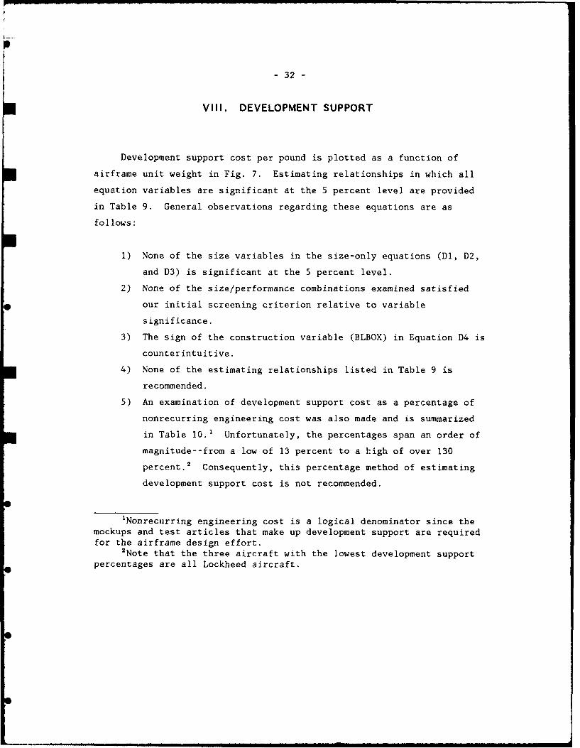
VIII. DEVELOPMENT SUPPORT

Development support cost per pound is plotted as a function of




follows:

1) None of the size variables in the size-only equations (Dl, D2,

and D3) is significant at the 5 percent level.

2) None of the size/performance combinations examined satisfiedour initial screening criterion relative to variable

significance.

3) The sign of the construction variable (BLBOX) in Equation D4 is

counterintuitive.


recommended.

5) An examination of development support cost as a percentage of

nonrecurring engineering cost was also made and is summarized

in Table 10.1 Unfortunately, the percentages span an order of

magnitude--from a low of 13 percent to a high of over 130

percent. 2 Consequently, this percentage method of estimating

development support cost is not recommended.

'Nonrecurring engineering cost is a logical denominator since themockups and test articles that make up development support are requiredfor the airframe design effort.

2Note that the three aircraft with the lowest development supportpercentages are all Lockheed aircraft.

-33-

9.0

8.5 0 B-58

0

a)8.0

0

A.-

3:7.50ORB-66

0. a.2 E KC-135 0

C-133 00'-

0E

6.5 Based on Eq. D1(without B-58)

0S

z 6.0

0OC-13005.5 1

10.0 10.5 11.0 11.5 12.0 12.5 13.0


Fig. 7-Development support cost per pound as a functionof airframe unit weight

-34-

0l- 0 a0 xU ~ w- W)~ Ui- 0 M 0 0

E .. o U..-o O-.o U00

C.~."C 0~*' 0.' 30 0

0 >cl- rf-m Cj- U(l ..

7 1.11 0.11 all

< I<

\. CQa) 0+

<I +

ccJ 0 LI co r N0 Ij Ij Io\0

Cm*

0

x 0.Ul

.0O Cfl C

(N ODf C.N w. 00 * 3:

i-* 0

00.~u 01 Ln00 'CO (L

0 W

0z in 0

- 35 -

Tqble 10

DEVELOPMENT SUPPORT COST AS A PERCENTAGE OF UNIT 1 ENGINEERING COST

Unit 1 Unit 1 Development Dev Support asEngineering Engineering Support a Percentage of

Aircraft Hours Cost ($M)(a) Cost ($M) Unit 1 Engr Cost

B-52 5,800,000 159.5 105.5 66B-58 3,150,000 86.6 165.1 191B/RB-66 1,600,000 44.0 53.0 120C-5 23,200,000 651.8 138.5 21C-130 3,350,000 92.1 12.3 13C-133 3,000,000 82.5 101.6 123KC-135 2,500,000 68.8 90.6 132C-141 6,800,000 187.0 47.5 25

(a)At $27.50 per hour.

0

*2

36 -

IX. FLIGHT TEST

Flight test cost per aircraft is plotted as a function of the

quantity of flight test aircraft in Fig. 8. Estimating relationships in

which all equation variables are significant at the 5 percent level are

provided in Table 11. As indicated, we were not able to identify any

estimating relationships which satisfied our initial screening criterion

relative to variable significance.

i

0

- 37 -

17.00 B-52

16.5

B-58 0

16.0 -

0 C-141C.

0 0 C-50

15.5 0K-315K 3Based on Eq. F1

'SP (without B-58)

Ezii

c) 15.00

z

14.5 0 C-1300 RB-66

14.0 I I1.5 2.0 2.5 3.0 3.5

Natural logarithm of quantity of flight test aircraft

Fig. 8-Flight test cost per test aircraft as a functionof the quantity of flight test aircraft

LI

-38-

o)

(n_ I

400c

oa

z CD

- 0w - %

z- CD

<C CfL

00 £

00

(30

IA 0N<

(< 0

Li C /) L ) C

0 z L

0 0

- 39 -

X. QUALITY CONTROL

Quality control hours per pound are plotted as a function of

airframe unit weight in Fig. 9. The data, which do not fit any obvious

patterns, are available for only five aircraft (four excluding the

B-58). Consequently, regression analysis does not seem appropriate.

However, since quality control is closely related to direct

manufacturing labor, it can be estimated as a percentage of same. The

ratio of cumulative quality control hours to cumulative manufacturing

labor hours is as follows:

Aircraft Ratio (at Q=100)

B-S2 .095B-58 .163C-5 .097C-141 .054KC-135 .103

Average, all aircraft .102Average, excluding B-58 .087

Excluding the B-58, the ratio of cumulative quality.control hours tocumulative manufacturing labor hours spans a range of 5.4 percent to10.3 percent with an average of 8.7 percent. 0

• m •

4n

1.0

0 B-580.5

EZ

'-oC0CL

- 00(n:3

00

Co0

EE 0 B-52

CZ Z -1.0 KC-1350a .Fz 0 C-5

z

-1.5

-2.0 I 0C-141

10.0 10.5 11.0 11.5 12.0 12.5 13.0


Fig. 9-Quality control hours per pound as a functionof airframe unit weight

- 41 -

Xl. TOTAL PROGRAM COST

Total program cost per pound is plotted as a function of airframe

unit weight in Fig. 10. Estimating relationships in which all equation



Only one size/performance variable combination (EW/USELD)

satisfied our initial screening criterion relative to variable

significance. However, the sign of the performance variable

exponent is counterintuitive.

0 Only one size/construction, program variable combination

satisfied our initial screening criterion relative to variable

significance. However, the magnitude of the construction

variable (AVAUW) exponent seems too large--each doubling of the

avionics weight to airframe unit weight ratio results in a 32

percent increase in total program cost. Such a result may be

reasonable for fighters but does not seem so for large,

subsonic aircraft.

The fit of the three size-only equations (PI, P2, and P3) is

determined largely by the B/RB-66. If the B/RB-66 were

excluded from the sample, no discernible trend would exist (see

Fig. 10).

None of the estimating relationships listed in Table 12 is

recommended.

- -

- 42 -

7.0

0 B-58

6.8 -

6.6

0

.- 6.4

000-E 6.2

O RB.66

@ ? 6.0

z " E /Based on Eq. P1

: 5.8 (without B-58)

cu OB-52o~5.6 - C-1 30 0

" 5.4 - 0 KC-135 0 C-5

5.2 - 0 C-141

5.0 1 1 1 1 1

10.0 10.5 11.0 11.5 12.0 12.5 13.0


Fig. 10-Total program cost per pound as a functionof airframe unit weight

-43-

V W 0 ulu I

0 O..O-D 0C~

> W lLi.J

0 '0 c \.0c

(n I CD<z 100

o + 0 +X

- a-, +

CL-

I,, C ~ N

co o - N 0

4) V V + +

< it' +~ Mco00

40 -21

(V~~- LiN -4.)J

i(A

wo (7 C )CCc

:300 x0 r ' '

Lfl 0

0~1 0

<00 -

L-- 0 - ) C

Zt' CLC.C

-44-

XII. CONCLUSIONS

We were not able to identify any acceptable estimating

relationships for any of the individual cost elements or for total

program cost. We suggest that users develop estimates for proposed

bomber/transport aircraft either on the basis of analogy (using the data

provided in this volume) or by using the equation set developed for all

mission types.

We believe that our inability to develop a set of statistically

derived cost-estimating relationships for bomber/transport aircraft is

the result of a sample that is both small and not as homogeneous as it

appears at first glance. For example:

* The B-58 is a Mach 2 aircraft while all other aircraft in the

sample are subsonic;

* The C-130 and C-133 are propeller-driven aircraft;

o The B/RB-66 and KC-135 were evolutionary developments;

* The B-52 was into its fourth series (the "D" version) by the

time 100 aircraft had been produced;

* The C-141 had a very large percent of subcontract effort

(approximately 50 percent), which may have distorted the

distribution of equivalent in-plant cost (Ref. 2, p. 50);

* The C-5 program utilized the acquisition concepts of total

package procurement and concurrent development and production.

Given this amount of diversity in so small a sample, it would have been

surprising if we had been able to develop a credible set of CERs.

COST-QUANTITY SLOPES

Minimum, maximum, and average cost-quantity slopes for the

bomber/transport subsample (excluding the B-58) are provided in Table

13

- 45 -

Table 13

CUMULATIVE TOTAL COST QUANTITY SLOPES

Mfg Mfg Quality TotalEngineering Tooling Labor Material Control Program

Number ofobservations 7 7 7 7 4 7

Range (%) 110-116 108-122 146-168 160-182 146-158 130-138Average (%) 114 114 154 168 152 136Exponent .189 .189 .623 .748 .604 .444

NOTES: Results are based on first 200 units; sample excludes B-58;cumulative average slope = cumulative total slope divided by two.

FULLY BURDENED LABOR RATES

All cost elements estimated directly in dollars are in 1977

dollars. Suggested 1977 fully burdened hourly labor rates (and those

used to estimate total program cost) are:

Engineering 27.50Tooling 25.50Manufacturing labor 23.50Quality Control 24.00

For estimates in 1986 dollars, the following hourly labor rates and

adjustment factors are suggested:

Engineering 59.10Tooling 60.70Manufacturing labor 50.10Quality control 55.40Manufacturing material (index) 1.94Development support (index) 1.94Flight test (index) 1.94 STotal program (index) 2.13

I

- 46 -

The 1986 labor rates are based on data provided by seven contractors:

Hourly Rates ($)

Labor Range AboutCategory Average Range Average (%)

Engineering 59.10 47.70-70.00 -19, +18Tooling 60.70 56.50-65.00 7, +7Manufacturing labor 50.10 41.70-58.00 -17, +16Quality control 55.40 49.10-62.60 -11, +13

Note that with tne exception of tooling, the range about the average

rate is at least ±10 percent. Such differences could arise from

differences in accounting practices, business bases, and capital

investment. Irrespective of cause, however, labor rate variation is one

more component of a larger uncertainty which already includes the error

associated with statistically derived estimating relationships and

questions about the proper cost-quantity slope. Furthermore, in

addition to the inter-contractor differences, these rates are also

subject to temporal change--accounting procedures, relative

capital/labor ratio, etc. Thus, the 1986 fully burdened rate is

qualitatively different from the 1977 rate. Unfortunately, trying to

estimate the magnitude of such quality changes, even very crudely, is a

study in itself and beyond the scope of this analysis.

The material, development support, and flight test escalation

indexes are based on data provided in AFR 173-13.1 For the years

1977-1984, the airframe index presented in Table 5-3 ("Historical

Aircraft Component Inflation Indices") was used. For the years 1985 and

1986, the aircraft and missile procurement index presented in Table 5-2

("USAF Weighted Inflation Indices Based on OSD Raw Inflation and Outlay

Rates") was used. The total program cost adjustment factor was then

determined on the basis of a weighted average (at Q 100) of the

individual cost elements.

'See Ref. 6.

- 47 -

Appendix 4

CORRELATION MATRIXES

This appendix contains correlation matrixes for the full

bomber/transport estimating sample. Table A.1 provides Pearson

correlation coefficients for all possible pairwise combinations of

dependent and independent variables. Table A.2 provides coefficients

for all possible pairwise combinations of independent variables.

0

0

- 48 -

Table A. 1

CORRELATION MATRIX: COST VARIABLES WITHPOTENTIAL EXPLANATORY VARIABLES

EXPLANATORY COST VARIABLES

VA RIABL ZES A~. 'AJn A A -A.ENGR TOOL LA8'R MATL Ds 07 PROG

SIZE

41W 0.58 0.37 0.80 07/ 035 il 066

,? EW 0.C3 0.46 083 077 042 0.26 0.72

WTAFEA 0.58 0.35 0.77 0.72 0.31 0.14 0.64PERPV'MA NCE

,3P 059 06 4 0.// 033 0.55 0.72 041

SPCLS 042 0.36 -0.02 0.23 0.41 0.6/ 028

eZ C/IMB 045 04.3 0.090 0.32 0.43 0 42 032

IUSELD 0.2?8 0.24 006 0.2S 0.56 055 0.23

CONS'TRC 7ION

Z /LTLD -06/ -0.43 -029 -0.61 -040 -0.84 -0.5/

SWG7Y'PE 0.39 0.70 0, 25 0.40 060 065 0.49

W W T 0.4s 0. 0 -009 0.37 0.16 0.66 022

EWA'IW -0.16 0.13 -0.44 -0/7 003 o5s -0.18

1AVAt1W -0.65 0.05 -041 -049 -0.17 0.20 -0.37

,? BLSOX 0.86 0.63 0.-1 0.87 0.40 0.59 0.75

PRO GR4 At

, TEST, C 0.22 052 0.12 0./2 0.44 062 0.30

, 0 TOOLCP -0.49 -032 -0.76 -0.45 -0.55 -. 07 -0.59

A ENGDV 0.18 0.27 0.32 0.14 0. O 0.21/ 028

'EPDoV 0/7 -0.13 -0.36 -0/14 -0.34 0.// -0.13

PRADV - 028 -0.12 -032 -0/14 -0.38 003 -0.28

S

S

- 49 -

>4

. . ii"- -

1-4 _ _ _ _ _ _ _ _ _ _ _ _ _ _ _ _ _

p- -4 Q

P-4

1-4

-4 r4

I •

Qi 0 Q0

,-I -4I I I II S 5

I I I I

14 :

14 '

- 51 -

REFERENCES

1. Levenson, G. S., and S. M. Barro, Cost-Estimating Relationships forAircraft Airframes, The RAND Corporation, RM-4845-PR, February 1966(out of print).

2. Levenson, G. S., H. E. Boren, Jr., D. P. Tihansky, and F. Timson,Cost-Estimating Relationships for Aircraft Airframes, The RANDCorporation, R-761-PR, December 1971 (For Official Use Only)(Privileged Information).

3. Large, Joseph P., Harry G. Campbell, and David Gates, ParametricEquations for Estimating Aircraft Airframe Costs, The RANDCorporation, R-1693-l-PA&E, February 1976.

4. Green, William, The World's Fighting Planes, Doubleday and Company,

Garden City, New York, 1964.

5. Bor-n. F. E., Jr., A C-"puter Model for Estimating Development andProcurement Costs of Aircraft (DAPCA-III), The RAND Corporation,R-1854-PR, March 1976.

6. U.S. Air Force Cost and Planning Factors, AFR 173-13, Department ofAir Force, Headquarters USAF, Washington, D.C., February 1, 1985(updates through Change 3, January 31, 1986).

0

0

S

S

rand - defense technical information center · a rand note n-2283/3-af aircraft airframe cost...

Documents