ramsey monetary policy with labour market frictions1

ISSN 1561081-0

9 7 7 1 5 6 1 0 8 1 0 0 5

WORKING PAPER SER IESNO 707 / JANUARY 2007

RAMSEY MONETARY POLICY WITH LABOUR MARKET FRICTIONS

by Ester Faia

In 2007 all ECB publications

€20 banknote.

WORK ING PAPER SER IE SNO 707 / JANUARY 2007

This paper can be downloaded without charge from http://www.ecb.int or from the Social Science Research Network

electronic library at http://ssrn.com/abstract_id=654699.

RAMSEY MONETARY POLICY WITH LABOUR

MARKET FRICTIONS 1

by Ester Faia 2

1 I gratefully acknowledge financial support from the DSGE grant. This paper was completed during my visit at the Directorate General Research of the European Central Bank. All errors are my own responsibility.

2 Department of Economics, Universitat Pompeu Fabra, Ramon Trias Fargas 25-27, 08005 Barcelona, Spain; e-mail: [email protected]. Homepage: http://www.econ.upf.edu/~faia.

feature a motif taken from the

© European Central Bank, 2007

AddressKaiserstrasse 2960311 Frankfurt am Main, Germany

Postal addressPostfach 16 03 1960066 Frankfurt am Main, Germany

Telephone +49 69 1344 0

Internethttp://www.ecb.int

Fax +49 69 1344 6000

Telex411 144 ecb d

All rights reserved.

Any reproduction, publication and reprint in the form of a different publication, whether printed or produced electronically, in whole or in part, is permitted only with the explicit written authorisation of the ECB or the author(s).

The views expressed in this paper do not necessarily reflect those of the European Central Bank.

The statement of purpose for the ECB Working Paper Series is available from the ECB website, http://www.ecb.int.

ISSN 1561-0810 (print)ISSN 1725-2806 (online)

3ECB

Working Paper Series No 707January 2007

CONTENTS

Abstract 4Non-technical summary 51 Introduction 62 The model economy 8 2.1 Households 9 2.2 The production sector 10 2.2.1 Search and matching in the labor market 10 2.2.2 Monopolistic f irms 11 2.2.3 Bellman equations, wage setting and Nash bargaining 12 2.3 Equilibrium conditions 133 The optimal policy problem 13 3.1 The role of frictions in this economy 14 3.2 The optimal policy problem under commitment 16 3.2.1 Non-recursivity and initial conditions 17 3.3 Calibration 184 Steady state optimal policy 195 Optimal stabilization policy and welfare 20 5.1 Dynamic of the optimal policy in response to shocks 20 5.2 Comparison between Ramsey policy and policy rules 22 5.3 Optimal volatility of inflation 22 5.4 Adding real wage rigidity 236 Conclusion 237 Appendix A – The stationary Lagrangian problem 25References 26Figures 29European Central Bank Working Paper Series 34

4ECB Working Paper Series No 707January 2007

Abstract

This paper studies the design of optimal monetary policy (in terms of unconstrained Ramseyallocation) in a framework with sticky prices and matching frictions. Furthermore I consider therole of real wage rigidities. Optimal policy features significant deviations from price stabilityin response to various shocks. This is so since search externalities generate an unemploy-ment/inflation trade-off. In response to productivity shocks optimal policy is pro-cyclical whenthe worker’s bargaining power is higher than the share of unemployed people in the matchingtechnology and viceversa. This is so since when the workers’ share of surplus is high there aremany searching workers and few vacancies hence the monetary authority has an incentive to in-crease vacancy profitability by reducing the interest rate and increasing inflation. The oppositeis true when the workers’ share of surplus is high. This implies that optimal inflation volatilityis U-shaped with respect to workers’ bargaining power.

JEL Codes: E52, E24Keywords: optimal monetary policy, matching frictions, wage rigidity.

Non-Technical Summary

This paper derives optimal monetary policy in a model economy characterized by monopolisticcompetition and adjustment costs on pricing and matching frictions in the labour market. Further-more I will also consider the role of real wage rigidity. Several papers in the recent literature studythe effects of introducing matching frictions in a New Keynesian framework but very little has beendone on the normative side. The assumption of monopolistic competition and adjustment cost onpricing a’ la Rotemberg (1982) is needed to obtain non-neutral effects of monetary policy and tomake a meaningful comparison across different monetary policy regimes. Introducing matchingfrictions a’ la Mortensen and Pissarides (1999) in the labor market allows to consider frictionalunemployment in the steady state and provides a rich dynamics for the formation and dissolutionof employment relations. Finally the reason for considering the effects on the optimal policy designof real wage rigidity is twofold. First, several authors have argued that real wage rigidity helpsto recover the typical unemployment-inflation trade-off commonly faced by central banks. Suchtrade-off, absent in standard new-keynesian models, is an essential feature to determine whetheroptimal monetary policy should deviate from full price stabilization. Secondly, some authors haveshown that the introduction of real wage rigidity helps to resolve some inconsistencies betweenthe standard matching friction model and the empirical evidence. The design of optimal policyin this paper follows the Ramsey approach according to which the monetary authority sets theoptimal path of all variables in the economy by maximizing agents’ welfare subject to the relationsdescribing the competitive economy.

The economy described is characterized by three sources of inefficiency, both in the long andin the short run. The first is monopolistic competition which induces an inefficiently low level ofoutput thereby calling for mild deviations from strict price stability1. The second type of distortionstems form the cost of adjusting prices which reduces output resources thereby calling for closing the“inflation gap”. Finally the search theoretic framework is characterized by a congestion externalitythat tends to tighten the labour market. The chance that workers and firms have to match dependson the number of unemployed people or vacant firms in the market. Whether there is excessivevacancy creation or excessive unemployment depends on the bargaining power of workers: whenthe latter (hence the workers’ share in the matching surplus) is too small there will be excessivevacancy creation due to the high profitability of a match for the firm and viceversa. In generalHosios (1990) has shown that the distance between current and efficient employment increaseswhen the distance between workers’ bargaining power and the fraction of searchers in the matchingtechnology increases.

Optimal policy features significant deviations from price stability in response to various shocks.This is so since search externalities generate an unemployment/inflation trade-off which induces themonetary authority to strike a balance between reducing the cost of adjusting prices and increasingan inefficiently low employment. In response to productivity shocks optimal policy is pro-cyclicalwhen the worker’s bargaining power is higher than the share of unemployed people in the matchingtechnology and viceversa. This is so since when the workers’ share of surplus is high (firms’ shareis low) there are many searching workers and few vacancies hence the monetary authority has anincentive to increase vacancy profitability by reducing the interest rate and increasing inflation.The opposite is true when the workers’ share of surplus is high. This also implies that optimal

1See Schmitt-Grohe and Uribe (2004) and Faia (2005) among others.

inflation volatility is U-shaped with respect to workers’ bargaining power.

5ECB


1 Introduction

Most central banks face an inflation-unemployment trade-off which implies that price stabilization

can be achieved at the cost of higher unemployment. Moreover the ratio between the cost of

inflation and the cost of unemployment is typically an increasing function of the degree of labor

market rigidity. The trade-offs described suggest that the optimal monetary policy design should

strike a balance between stabilizing inflation and fighting low employment. However most of the

recent literature on the design of monetary policy concludes that optimality features either zero

inflation or small deviations from price stability. This result has been established under different

settings and characterizes both the closed and the open economy context1. One shortcoming of

those studies is the lack of labor market rigidities which are a key ingredient in generating steady

state unemployment and in characterizing employment fluctuations.

This paper derives optimal monetary policy in a model economy characterized by monopolistic

competition and adjustment costs on pricing and matching frictions in the labour market. Further-

more I will also consider the role of real wage rigidity. Several papers in the recent literature study

the effects of introducing matching frictions in a New Keynesian framework but very little has been

done on the normative side. The assumption of monopolistic competition and adjustment cost on

pricing a’ la Rotemberg (1982) is needed to obtain non-neutral effects of monetary policy and to

make a meaningful comparison across different monetary policy regimes. Introducing matching

frictions a’ la Mortensen and Pissarides (1999) in the labor market allows to consider frictional

unemployment in the steady state and provides a rich dynamics for the formation and dissolution

of employment relations2. Finally the reason for considering the effects on the optimal policy design

of real wage rigidity is twofold. First, several authors have argued that real wage rigidity helps

to recover the typical unemployment-inflation trade-off commonly faced by central banks3. Such

trade-off, absent in standard new-keynesian models, is an essential feature to determine whether

optimal monetary policy should deviate from full price stabilization. Secondly, some authors have1Zero inflation is the core result in the analysis of Woodford (2003), Clarida, Gali and Gertler (2000) who consider

a monopolistic competitive framework with sticky prices a’ la Calvo (1983). Lately Khan, King and Wolman (2003)and Schmitt-Grohe and Uribe (2004) have shown, using the Ramsey approach, that in presence of sticky prices andmoney distortions optimal policy implies small deviations from price stability and departure from the Friedman rule.The same is true in presence of capital accumulation, see Faia (2005). Finally Adao, Correia and Teles (2003) haveshown by using a model with prices set one period in advance, that zero inflation is the optimal policy under a certainclass of preferences.

2The introduction of matching frictions into a new Keynesian model has become common in the recent literaturesince it allows to replicate some empirical features. The laboratory economy that I use is very close to the oneproposed in Krause and Lubik (2005). Several other authors, ranging from Walsh (2003) to Blanchard and Gali’(2005a,b), have recently introduced matching frictions and real wage rigidity into new Keynesian models.

3See Erceg, Henderson and Levin (2000), Canzoneri, Cumby and Diba (2004), and Blanchard and Gali’ (2005)among others.


shown that the introduction of real wage rigidity helps to resolve some inconsistencies between

the standard matching friction model and the empirical evidence4. The design of optimal policy

in this paper follows the Ramsey approach according to which the monetary authority sets the

optimal path of all variables in the economy by maximizing agents’ welfare subject to the relations

describing the competitive economy.

The economy described is characterized by three sources of inefficiency, both in the long and

in the short run. The first is monopolistic competition which induces an inefficiently low level of

output thereby calling for mild deviations from strict price stability5. The second type of distortion

stems form the cost of adjusting prices which reduces output resources thereby calling for closing the

“inflation gap”. Finally the search theoretic framework is characterized by a congestion externality

that tends to tighten the labour market. The chance that workers and firms have to match depends

on the number of unemployed people or vacant firms in the market. Whether there is excessive

vacancy creation or excessive unemployment depends on the bargaining power of workers: when

the latter (hence the workers’ share in the matching surplus) is too small there will be excessive

vacancy creation due to the high profitability of a match for the firm and viceversa. In general

Hosios (1990) has shown that the distance between current and efficient employment increases

when the distance between workers’ bargaining power and the fraction of searchers in the matching

technology increases.

I find that the in general optimal policy should deviate from price stability in response to

different types of shocks. Contrary to previous studies deviations from the flexible price allocation

are quantitatively significant. This is so search externalities generate an unemployment/inflation

trade-off which induces the monetary authority to strike a balance between reducing the cost of

adjusting prices and increasing an inefficiently low employment.

In response to productivity shocks optimal policy is pro-cyclical when the worker’s bargaining

power is higher than the share of unemployed people in the matching technology and countercyclical

in the opposite case. The reason for this is as follows. When the workers’ share of surplus is high

and firms’ share is low there are many searching workers and few vacancies. In this case the

monetary authority has an incentive to increase vacancy profitability by reducing the interest rate

and increasing demand. This obviously comes at the cost of higher inflation. The opposite is true

when the workers’ share of surplus is high. In general I find that the optimal inflation volatility is

U-shaped with respect to workers’ bargaining power and for given share of unemployed workers in

the matching technology. In other words the monetary authority has an incentive to intervene and

4See Hall (2003), Shimer (2003) and Krause and Lubik (2005).5See Schmitt-Grohe and Uribe (2004) and Faia (2005) among others.

7ECB


reduce the search externality by manipulating inflation only when the distance between current

and efficient employment increases (e.g. when the distance between workers’ bargaining power and

the fraction of searchers in the matching technology increases).

The comparison between the dynamic under the Ramsey policy and the ones under other type

of operational rules shows that the first induces higher variability of all variables. Under the types

of rules considered, Taylor rule and the unemployment targeting, the monetary authority is only

concerned with stabilization. On the contrary the Ramsey planner has the incentive to take full

advantage of the productivity increase thereby exploiting all the benefits of the expansionary phase.

The findings in this paper are consistent with those in Cooley and Quadrini (2004). They study

Ramsey monetary policy, both under commitment and discretion, in an economy with matching

frictions and limited participation in financial market. Despite the fact that they have a different

transmission mechanism they also reach the conclusion that the optimal policy should be pro-

cyclical in response to productivity shocks when the worker’s bargaining power is higher than the

share of unemployed people in the matching technology.

Blanchard and Gali’ (2005) build a closed economy model with matching frictions and wage

rigidity and conduct some normative analysis. They find that the output/inflation trade-off induces

the monetary authority to deviate from strict inflation targeting. However their optimal policy

analysis is based on a microfounded loss function and a loglinear approximation of the competitive

equilibrium relations around a steady state where all distortions have been eliminated through an

appropriate choice of the parameter space. This implies that the emergence of the output/inflation

trade-off in their case is not directly related to the search externality, rather to the presence of

sticky wages as in Erceg, Henderson and Levin (2000).

The paper proceeds as follow. Section 2 presents the model. Section 3 analyzes the optimal

policy plan. Section 4 shows results for the long run optimal policy. Section 5 shows results for the

optimal policy along the dynamics. Section 6 concludes.

2 The Model Economy

There is a continuum of agents whose total measure is normalized to one. The economy is popu-

lated by households who consume different varieties of goods, save and work. Households save in

both non-state contingent securities and in an insurance fund that allows them to smooth income

fluctuations associated with periods of unemployment. Each agent can indeed be either employed

or unemployed. In the first case he receives a wage that is determined according to a Nash bargain-

ing, in the second case he receives an unemployment benefit. The labor market is characterized


by matching frictions and exogenous job separation. The production sector acts as a monopolistic

competitive sector which produces a differentiated good using labor as input and faces adjustment

costs a’ la Rotemberg (1982).

2.1 Households

Let ct ≡R 10 [(c

it)

−1di] −1 be a Dixit-Stiglitz aggregator of different varieties of goods. The op-

timal allocation of expenditure on each variety yields is given by ct =³pitpt

´−εct, where pt ≡R 1

0 [(pit)

−1di] −1 is the price index. There is continuum of agents who maximize the expected

lifetime utility6.

Et

( ∞Xt=0

βtc1−σt

1− σ

)(1)

where c denotes aggregate consumption in final goods. Households supply labor hours inelastically

h (which is normalized to 1). Total real labor income is given by wt and is specified below.

Unemployed households members, ut, receive an unemployment benefit, b. The contract signed

between the worker and the firm specifies the wage and is obtained through a Nash bargaining

process. In order to finance consumption at time t each agent also invests in non-state contingent

nominal bonds bt which pay a gross nominal interest rate (1+rnt ) one period later. As in Andolfatto

(1996) and Merz (1995) it is assumed that workers can insure themselves against earning uncertainty

and unemployment. For this reason the wage earnings have to be interpreted as net of insurance

costs. Finally agents receive profits from the monopolistic sector which they own, Θt, and pay

lump sum taxes, τ t. The sequence of real budget constraints reads as follows:

ct +btpt≤ wt + but +

Θt

pt− τ t

pt+ (1 + rnt−1)

bt−1pt

(2)

Households choose the set of processes {ct, bt}∞t=0 taking as given the set of processes {pt, wt, rnt }∞t=0

and the initial wealth b0,so as to maximize (1) subject to (2). The following optimality conditions

must hold:

λt = c−σt (3)

c−σt = β(1 + rnt )Et

½c−σt+1

ptpt+1

¾(4)

6Let st = {s0, ....st} denote the history of events up to date t, where st denotes the event realization at date t.The date 0 probability of observing history st is given by ρt. The initial state s

0 is given so that ρ0 = 1. Henceforth,and for the sake of simplifying the notation, let’s define the operator Et{.} ≡ st+1

ρ(st+1|st) as the mathematicalexpectations over all possible states of nature conditional on history st.

9ECB


Equation (3) is the marginal utility of consumption and equation (4) is the Euler condition with

respect to bonds. Optimality requires that No-Ponzi condition on wealth is also satisfied.

2.2 The Production Sector

Firms in the production sector sell their output in a monopolistic competitive market and meet

workers on a matching market. The labor relations are determined according to a standard

Mortensen and Pissarides (1999) framework. Workers must be hired from the unemployment pool

and searching for a worker involves a fixed cost. Workers wages are determined through a Nash

decentralized bargaining process which takes place on an individual basis.

2.2.1 Search and Matching in the Labor Market

The search for a worker involves a fixed cost κ and the probability of finding a worker depends on a

constant return to scale matching technology which converts unemployed workers u and vacancies

v into matches, m:

m(ut, vt) = muξtv1−ξt (5)

where vt =R 10 vi,tdi. Defining labor market tightness as θt ≡ vt

ut, the firm meets unemployed

workers at rate q(θ) = m(ut,vt)vt

= mθ−ξt , while the unemployed workers meet vacancies at rate

θtq(θt) = mθ1−ξt . If the search process is successful, the firm in the monopolistic good sector

operates the following technology:

yi,t = ztni,t (6)

where zt is the aggregate productivity shock which follows a first order autoregressive process,

ezt = eρzzt−1εz,t, and ni,t is the number of workers hired by each firm. Matches are destroyed at

an exogenous rate ρ7. We are now in the position to determine the law of motion for the workers

employed and the ones seeking for a job. Labor force is normalized to unity. The number of

employed people at time t in each firm i is given by the number of employed people at time t− 1plus the flow of new matches concluded in period t− 1 who did not discontinue the match:

ni,t = (1− ρ)(ni,t−1 + vi,t−1q(θi,t−1)) (7)

7The alternative assumption of endogenous job destruction would induce, consistently with empirical observations,additional persistence to the model as shown in denHaan, Ramsey and Watson (2000). However due to the normativefocus of this paper I choose the more simple assumption of exogenous job destruction. This greatly reduces thecomplexity of the numerical solution to the optimal policy problem without altering the results compared to thealternative assumption of endogenous job destruction. Indeed the main policy trade-offs do not change under thetwo alternative assumptions.


Unemployment is given by total labor force minus the number of employed workers:

ut = 1− nt (8)

Finally job creation rate is given by:

jct =(1− ρ)vt−1q(θt−1)

nt−1(9)

2.2.2 Monopolistic Firms

Firms in the monopolistic sector use labor to produce different varieties of consumption good and

face a quadratic cost of adjusting prices. Wages are determined through the bargaining problem

analyzed in the next section. Here I develop the dynamic optimization decision of firms choosing

prices, pih,t, number of employees, ni,t, number of vacancies, vi,t, to maximize the discounted value of

future profits and taking as given the wage schedule. The representative firm chooses©pit, ni,t, vi,t

ªto solve the following maximization problem (in real terms):

MaxΠi,t = E0

∞Xt=0

βtλtλ0

(pitptyit − wi,tni,t − κvi,t −

ψ

2

µpitpit−1

− 1¶2

yit

)(10)

subject to

s.to: yit =

µpitpt

¶−yt = ztni,t (11)

and: ni,t = (1− ρ)(ni,t−1 + vi,t−1q(θi,t−1)) (12)

where ψ2

³pit

pit−1− 1´2

yit represent the cost of adjusting prices, ψ can be thought as the sluggishness

in the price adjustment process, κ as the cost of posting vacancies and wt denotes the fact that the

bargained wage might depend on time varying factors. Let’s define mct, the lagrange multiplier

on constraint (11), as the marginal cost of firms and µt, the lagrange multiplier on constraint (12),

as the marginal value of one worker. Since all firms will chose in equilibrium the same price and

allocation we can now assume symmetry and drop the index i. First order conditions for the above

problem read as follows:

• nt :

µt = mctzt − wt + βEt(λt+1λt

)((1− ρ)µt+1) (13)

• vt :κ

q(θt)= βEt(

λt+1λt

)((1− ρ)µt+1) (14)

11ECB


• pt :

1− ψ(πt − 1)πt + βEt(λt+1λt

)[ψ(πt+1 − 1)πt+1yt+1yt] = (1−mct)ε (15)

Merging equations (13) and (14) rearranging we obtain the marginal cost of firms, mct,:

mct =µt− κ

q(θt)

zt+

wt

zt(16)

As already noticed in Krause and Lubik (2005) in a matching model the marginal cost of firms

is not only given by the marginal productivity of each single employee, wtzt, as it is in a standard

walrasian model but contains an extra component,µt− κ

q(θt)

zt,which depends on the future value of

each employee. Posting vacancy is costly hence a successful match today is valuable also since it

reduces future search costs.

2.2.3 Bellman Equations, Wage Setting and Nash Bargaining

The wage schedule is obtained through the solution to an individual Nash bargaining process. To

solve for it we need first to derive the marginal values of a match for both, firms and workers.

Those values will indeed enter the sharing rule of the bargaining process. Let’s denote by V Jt the

marginal discounted value of a match for a firm:

V Jt = mctzt − wt +Et{(β

λt+1λt

)[(1− ρ)V Jt+1]} (17)

The marginal value of a match depends on real revenues minus the real wage plus the dis-

counted continuation value. With probability (1− ρ) the job remains filled and earns the expected

value and with probability, ρ, the job is destroyed and has zero value. Using the equation (16) we

can rewrite equation (17) as:

V Jt =

−κq(θt)

+Et{(βλt+1λt

)[(1− ρ)V Jt+1]} (18)

Since the net value of a match for the firm must be zero in equilibrium the following zero profit

condition must be satisfied:

κ

q(θt)= Et{(β

λt+1λt

)[(1− ρ)V Jt+1]} (19)

Equation (19) is an arbitrage condition for the posting of new vacancies. It implies that in

equilibrium the cost of posting a vacancy must equate the discounted expected return from posting

the vacancy. For each worker, the values of being employed and unemployed are given by V Et and

V Ut :

V Et = [wt +Et{(β

λt+1λt

)[(1− ρ)V Et+1 + ρV U

t+1]} (20)


V Ut = [b+Et{(β

λt+1λt

)[θtq(θt)(1− ρ)V Et+1 + (1− θtq(θt)(1− ρ))V U

t+1]} (21)

where b denotes real unemployment benefits.

Workers and firms are engaged in a Nash bargaining process to determine wages. The optimal

sharing rule of the standard Nash bargaining is given:

(V Et − V U

t ) =ς

1− ςV Jt (22)

After substituting the previously defined value functions it is possible derive the following wage

schedule:

wt = ς(mctzt + θtκ) + (1− ς)b (23)

2.3 Equilibrium Conditions

Aggregate output is obtained by aggregating production of individual firms. I assume that there

is exogenous government expenditure financed through lump sum taxation. Hence the resource

constraint reads as follows:

yt = ntzt = ct + gt + κvt +ψ

2(πt − 1)2 yit (24)

Furthermore I assume zero total net supply of bonds.

Definition 1. A distorted competitive equilibrium for this economy is a sequence of allocation

and prices {ct, ut, nt, vt, θt, πt, yt, wt, rnt ,mct}∞t=0 which, for given initial B0 satisfies equations

(4),(7),(8),(13),(14),(15),(23),

(24) and θt ≡ vtut.

3 The Optimal Policy Problem

The optimal policy is determined by a monetary authority that maximizes the discounted sum of

utilities of all agents given the constraints of the competitive economy. The next task is to select

the relations that represent the relevant constraints in the planner’s optimal policy problem. This

amounts to describing the competitive equilibrium in terms of a minimal set of relations involving

only real allocations, in the spirit of the primal approach described in Lucas and Stokey (1983).

There is a fundamental difference, though, between that classic approach and the one followed

here, which stems from the impossibility, in the presence of sticky prices and matching frictions,

of reducing the planner’s problem to a maximization only subject to a single implementability

constraint8.8See also Khan, King and Wolman (2003), Schmitt-Grohe and Uribe (2002) and Faia (2005).

13ECB


The first order conditions of the consumers can be summarized as follows:

c−σt = β(1 + rnt )Et

½c−σt+1

ptpt+1

¾(25)

The first order conditions and the constraints of the production sector can be summarized as

follows:

1− ψ(πt − 1)πt + βEt(ct+1ct)−σ[ψ(πt+1 − 1)πt+1

yt+1yt] = (1−mct)ε (26)

κ

mθξt = Et{β(

ct+1ct)−σ(1− ρ)[(1− ς)mct+1zt+1 − ςθt+1κ− (1− ς)b+

κ

mθξt+1]} (27)

where θt ≡ vtutand ut = 1− nt. Finally need to include the resource constraint and the employment

dynamic:

ntzt = ct + gt + κvt +ψ

2(πt − 1)2 yt (28)

nt = (1− ρ)(nt−1 + vt−1muξtv1−ξt ) (29)

3.1 The Role of Frictions in This Economy

As discussed previously this economy is characterized by three main frictions: price stickiness,

monopolistic competition and matching frictions in the labor market. A monetary policy maker

endowed with a single instrument is not able eliminate all the three distortions but can only trade-

off among them. To better understand the type of trade-offs present in this model economy it is

useful to discuss the role of each friction singularly and the level of the policy instrument required

to offset them.

I start by analyzing the role of matching frictions in the labor market since they provide the

novel aspect for the design of the optimal policy in the context of new keynesian models. To

understand how search externality distort the competitive equilibrium let’s assume for simplicity

that those are the only frictions characterizing the model economy and let’s derive the conditions

for constrained pareto efficiency. The optimal policy problem of the planner in this context (and

in absence of government expenditure) can be written as follows:

MaxEt

( ∞Xt=0

βtc1−σt

1− σ

)(30)

s. to

ztnt − κvt = ct (31)


nt = (1− ρ)(nt−1 + vt−1q(θt−1)) (32)

where θt ≡ vtut, ut = 1 − nt and q(θ) = mθ−ξt . Let’s define as ψ1,t and ψ2,t respectively the

lagrange multipliers on constraints (31) and (32). First order conditions for this problem are as

follows:

• ct :

c−σt − ψ1,t = 0 (33)

• nt :

ψ1,tzt − ψ2,t+1(1− ρ)mv1−ξt+1 ξ(1− nt+1)ξ−1 + ψ2,t+1 = 0 (34)

• vt :

−ψ1,tκ− ψ2,tm(1− nt)ξ−1(1− ρ)(1− ξ)v−ξt = 0 (35)

After rearranging and merging the above first order conditions we obtain the following:

κ

mθξt = Et{β(

ct+1ct)−σ(1− ρ)[(1− ξ)mct+1zt+1 − ξθt+1κ− (1− ξ)b+

κ

mθξt+1]} (36)

Notice that equation (36) is equivalent to (27) when ξ = ς. This is exactly the condition

that Hosios (1990) suggests to achieve constrained pareto efficiency in an economy with matching

frictions. Efficiency requires workers’ bargaining power being equivalent to their share in the

matching technology. When workers bargaining power is too low (ξ ≤ ς) firms find too profitable

to form a match thereby inducing excessive vacancy creation. Viceversa, when workers’ bargaining

power is too high there is excessive unemployment. If the condition for efficiency are not met an

obvious solution is to endow the policy maker with a complementary subsidy that forces ξ = ς. As

we shall see below in absence of such subsidy the monetary authority can use inflation to control

for the optimal level of unemployment in the economy.

Let’s now consider the role of price stickiness and monopolistic competition. Price stickiness

induces a gap with the flexible price allocation since part of resources are wasted in the activity of

adjusting prices, (πt − 1)2 . Finally monopolistic competition reduces the level of economic activityby decreasing optimal demand, hence the marginal cost to firms (see also Schmitt-Grohe and Uribe

(2004)).

We are now in the position to determine the level of the policy instrument which can offset

each distortion at the time. Obviously the cost of adjusting prices can be eliminated by setting

πt = 1 at all times, thereby following a strict price stability policy. From the Phillips curve it

is obvious that an increase in the marginal cost (hence a reduction of mark-up and an increase

15ECB


in demand) can be achieved by setting positive inflation. Both price stickiness and monopolistic

competition can be directly affected by the inflation level. As for the matching frictions the policy

maker can have only an indirect impact on those externalities by using inflation. Consider the

marginal discounted value of a match for a firm:

V Jt = mctzt − wt +Et{(β

λt+1λt

)[(1− ρ)V Jt+1]} (37)

After solving recursively we obtain:

V Jt =

∞Xj=0

Et+j{βλt+j+1λt+j

(1− ρ)Πt+j} (38)

where Πt+j = mct+jzt+j − wt+j . Since the discounted value of a match must equate the cost

of posting vacancy discounted by the probability of filling a vacancy we can also conclude that:

κ

q(θt)=

∞Xj=0

Et+j{βλt+j+1λt+j

(1− ρ)Πt+j} (39)

A reduction in the mark-up (or an increase in demand and marginal costs) achieved through

an increase in inflation can increase unitary profits, Πt+j = mct+jzt+j − wt+j ,at each point in

time. An increase in unitary profits, for given cost of posting vacancy κ, can reduce labor market

tightness, q(θt),thereby reducing the congestion externality. Positive inflation can therefore have

an indirect impact on the probability of forming matches through its impact on the demand for

varieties.

To summarize we have on the one side two distortions, monopolistic competition and search

externality, that call for positive inflation while we have on the other side a third distortion, price

stickiness, which calls for zero net inflation. Since the policy maker should trade-off among those

three distortions we expect the optimal policy to deviate from strict price stability.

3.2 The Optimal Policy Problem Under Commitment

I now turn to the specification of a general set-up for the optimal policy conduct.

Definition 2. Let {λ1,t, λ2,t, λ3,t, λ4,t, λ5,t}∞t=0 represent sequences of Lagrange multipliers onthe constraints (25), (26), (27), (28) and (29) respectively. Then for given stochastic processes

{zt, gt}∞t=0 and for given B0 plans for the control variables {ct, nt, vt, πt, rnt ,mct}∞t=0 and for theco-state variables {λ1,t, λ2,t, λ3,t, λ4,t, λ5,t}∞t=0 represent a first best constrained allocation if theysolve the following maximization problem:

Choose Λnt ≡ {λ1,t, λ2,t, λ3,t, λ4,t, λ5,t}∞t=0 and Ξnt ≡ {ct, nt, vt, πt, rnt ,mct}∞t=0 to


Min{Λnt }∞t=0

Max{Ξnt }∞t=0

E0{∞Xt=0

βtEt{U(Ct, Nt) (40)

+λ1,t

∙c−σt − β(1 + rnt )Et

½c−σt+1

1

πt+1

¾¸+

+λ2,t[1− ψ(πt − 1)πtytct + βEt(ct+1)−σ[ψ(πt+1 − 1)πt+1yt+1]− (1−mct)ctytε] +

+λ3,t

∙κ

mθξt −Et{β(

ct+1ct)−σ(1− ρ)[(1− ς)mct+1zt+1 − ςθt+1κ− (1− ς)b+

κ

mθξt+1]}

¸+

+λ4,t

∙ntzt − κvt −

ψ

2(πt − 1)2 yt − ct − gt

¸+

+λ5,t

hnt − (1− ρ)(nt−1 + vt−1muξtv

1−ξt )

i}}

where θt ≡ vtutand ut = 1− nt

3.2.1 Non-recursivity and Initial Conditions

As a result of the constraint (25), (26) and (27) exhibiting future expectations of control variables,

the maximization problem as spelled out in (40) is intrinsically non-recursive.9 As first emphasized

in Kydland and Prescott (1980), and then developed by Marcet and Marimon (1999), a formal way

to rewrite the same problem in a recursive stationary form is to enlarge the planner’s state space

with additional (pseudo) co-state variables. Such variables, that I denote χ1,t, χ2,t and χ3,tfor (25),

(26) and (27) respectively, bear the crucial meaning of tracking, along the dynamics, the value to the

planner of committing to the pre-announced policy plan. Another aspect concerns the specification

of the law of motion of these lagrange multipliers. For in this case both constraints feature a simple

one period expectation, the same co-state variables have to obey the laws of motion10:

χ1,t+1 = λ1,t (41)

χ2,t+1 = λ2,t

χ3,t+1 = λ3,t

9See Kydland and Prescott (1977), Calvo (1978). As such the system does not satisfy per se the principle ofoptimality, according to which the optimal decision at time t is a time invariant function only of a small set of statevariables.10The laws of motion of the additional costate variables would take a more general form if the expectations horizon

in the forward looking constraint(s) featured a more complicated structure, as, for instance, in the case of constraintsin present value form. See Marcet and Marimon (1999).

17ECB


Appendix A shows the stationary Lagrangian problem which is indeed recursive in the state

space {zt, gt, χ1,t, χ2,t , χ3,t}. To avoid time consistency problems and consistently with a timelessperspective I set the values of the three co-state variables at time zero equal to their solution in the

steady state. I will return on this point in the next subsection.

3.3 Calibration

Preferences. Time is measured in quarters. I set the discount factor β = 0.99, so that the annual

interest rate is equal to 4 percent. The parameter on consumption in the utility function is set

equal to 2.

Production. Following Basu and Fernald (1997) I set the value added mark-up of prices over

marginal cost to 0.2. This generates a value for the price elasticity of demand, ε, of 6. I set the cost

of adjusting prices ψ = 50 so as to generate a slope of the log-linear Phillips curve consistent with

empirical and theoretical studies.

Labor market frictions parameters. The matching technology is homogenous of degree

one function and is characterized by the parameter ξ. Consistently with estimates by Blanchard

and Diamond (1989) I set this parameter to 0.4. I set the steady state firm matching rate, q(θ), to

0.7 which is the value used by denHaan, Ramsey and Watson (1997). The probability for a worker

of finding a job, θq(θ), is set equal to 0.6, which implies an average duration of unemployment

of 1.67 as reported ion Cole and Rogerson (1996). With those values it is possible to determine

the number of vacancies as well as the vacancy/unemployment ratio. The exogenous separation

probability, ρ, is set to 0.08 consistently with estimates from Hall (1995) and Davis et al. (1996);

this value is also compatible with those used in the literature which range from 0.7 (Merz (1995)) to

0.15 (Andolfatto (1996)). The degree of wage rigidity, λ, is set equal to 0.6 and is compatible with

estimates from Smets and Wouters (2003). The value for b is set so as to generate a steady state

ratio, bw , of 0.5 which corresponds to the average value observed for industrialized countries (see

Nickell and Nunziata (2001)). The steady state scale paramter, m, is obtained using the observation

that steady state number of matches is given by ρ1−ρ(1− u). The bargaining power of workers, ς,is

set to 0.5 as in most papers in the literature, while the value for the cost of posting vacancies is

obtained from the steady state version of labour market tightness evolution.

Exogenous shocks and monetary policy: The process for the aggregate productivity

shock, zt, follows an AR(1) and based on the RBC literature is calibrated so that its standard

deviations is set to 0.008 and its persistence to 0.95. Log-government consumption evolves according

to the following exogenous process, ln³gtg

´= ρg ln

³gt−1g

´+ εgt , where the steady-state share of

government consumption, g, is set so that gy = 0.25 and εgt is an i.i.d. shock with standard


deviation σg. Empirical evidence for the US in Perotti (2004) suggests σg = 0.008 and ρg = 0.9.

4 Steady State Optimal Policy

Before turning to the optimal stabilization policy in response to shocks we need to characterize

the log-run optimal policy, which is the one to which the policy maker would like to converge.

To develop an analogy with the Ramsey-Cass-Koopmans model, this amounts to computing the

modified golden rule steady state. To determine the long-run inflation rate associated to the optimal

policy problem above, one needs to solve the steady-state version of the set of efficiency conditions.

Notice in particular that the first order condition with respect to inflation reads as follows:

(λ2,t − χ2,t)c−σt ψ(2πt − 1)yt − λ4,tψ (πt − 1) yt = 0 (42)

For the whole set of optimality conditions of the Ramsey plan to be satisfied in the steady state a

necessary condition is that equation (42) is satisfied in the steady state. In that steady-state, we

have λ2,t = λ2,t−1 = χ2,t. Hence condition (42) immediately implies:

λ4ψ (π − 1) y = 0 (43)

Since λ4 > 0 (the resource constraint must hold with equality), y > 0 and ψ > 0 (we are not

imposing a priori that the steady-state coincides with the flexible price allocation), in turn (43) must

imply π = 1. Hence the Ramsey planner would like to generate an average (net) inflation rate of

zero. The intuition for why the long-run optimal inflation rate is zero is simple. Under commitment,

the planner cannot resort to ex-post inflation as a device for eliminating the inefficiency related to

market power in the goods market. Hence the planner aims at choosing that rate of inflation that

allows to minimize the cost of adjusting prices, and summarized by the quadratic term ϑ2 (πt − 1)

2.

One may wonder why the search externality does not apparently exert any influence on the

desired optimal long-run inflation rate. In light of our considerations above, the desire of reducing

the congestion externality by increasing firms profits has been shown to be a sufficient motive for

inducing the planner to deviate from choosing a constant markup allocation. However, since the

policy maker can exert only an indirect effect on the search externality via a reduction in mark-up

and since it cannot resort to ex-post inflation as a device for eliminating the inefficiency related to

market power, we conclude that it is not possible under commitment to deviate from strict price

stability.

19ECB


5 Optimal Stabilization Policy and Welfare

Since we are mostly interested in the analysis of optimal policy along the business cycle we can

now analyze the optimal dynamic of variables in response to shocks. We focus on productivity and

government expenditure shocks. To solve for the optimal stabilization policy I compute second order

approximations11 of the first order conditions of the Lagrangian problem described in definition 2.

Technically I compute the stationary allocations that characterize the deterministic steady state

of the first order conditions to the Ramsey plan. I then compute a second order approximation

of the respective policy functions in the neighborhood of the same steady state. This amounts to

implicitly assuming that the economy has been evolving and policy has been conducted around

such a steady already for a long period of time (under timeless perspective).

Before proceeding with the quantitative analysis of the optimal policy it is worth noticing

that the competitive economy of the present model generates a volatility of unemployment which

is higher than the one featured by a standard new keynesian model and that the Beveridge curve

holds. Overall the model is able to account fairly well for the main stylized facts characterizing the

labor market12.

5.1 Dynamic of the Optimal Policy in Response to Shocks

Figure (1) shows impulse response of selected variables to productivity shocks. An increase in

productivity induces an increase in output. Optimal policy also features an increase in inflation (and

prices) to allow the economy to take full advantage of the higher productivity. Indeed a reduction

in the mark-up (or an increase in demand and marginal costs) achieved through an increase in

inflation can increase unitary profits, Πt+j = mct+jzt+j − wt+j ,at each point in time. An increase

in unitary profits, for given cost of posting vacancy κ, increases vacancy posting and reduces labor

market tightness, q(θt),thereby squeezing the congestion externality. As a consequence there is an

increase in employment as well. Positive inflation can therefore have an indirect positive impact

on the probability of forming matches through its impact on the demand for varieties. This is

beneficial on consumption and employment as well.

Figure (2) shows the response of the same set of variables to government expenditure shocks.

Optimal monetary policy implies in this case a fall in consumption and in the price level. The

government will want to have less consumption when government purchases are high since this

11Second order approximation methods have the particular advantage of accounting for the effects of volatility ofvariables on the mean levels of the same. See Schmitt-Grohe and Uribe (2004a,b) among others.12 In this context it is important to stress that the qualitative results concerning optimal policy (mostly the devia-

tions from price stability) remain the same independently from the calibration of the labor market parameters.


makes the state contingent claims value of the public spending high, making it easier to satisfy

monopoly producers. This argument is valid when the utility of the representative agent is separable

so that the price of the state contingent security only depends on consumption13. In order to

generate a fall in consumption the government increases the nominal interest rate and this also

implies a fall in the price level.

Importantly deviations from price stability are significant in response to both shocks. This

is in sharp contrast with the conclusions reached by previous studies of optimal policy which had

shown that deviations from price stability were nil or negligible mostly in response to productivity

shocks. In general it had been established that, in a context with monopolistic competition and

sticky prices, the constrained pareto optimum is reached by replicating the flexible price allocation

and that monetary policy should be neutral in response to productivity shocks. On the contrary

in our context optimal policy is in pro-cyclical in response to productivity shocks. With search

frictions indeed the level of employment is inefficiently low and a trade-off exists between inflation

and employment/output stabilization. In presence of such trade-off the monetary authority should

strike a balance between reducing the cost of adjusting prices and increasing employment.

A crucial determinant of the size and the direction of the congestion externality is the dis-

tance between the worker’s bargaining power and the share of unemployed people in the matching

technology. As mentioned before, Hosios (1990) had shown that efficiency can be achieved in a

matching model when workers’ bargaining power is equal to the share of unemployed people in

the matching technology. In different cases the labor market is tight, the probability of forming a

match is low and employment is inefficiently low. In general whenever the labor market features an

inefficiency the monetary authority has an incentive to intervene and deviate from price stability.

However when the bargaining power is high (for given share of unemployed people in the matching

technology), workers’ share of surplus is high (and firms’ share is low) and vacancies have little

profitability. In this case there is an excess of searching workers compared to the number of vacan-

cies. This increases labor market tightness and unemployment. Under those circumstances optimal

policy should be pro-cyclical since an increase in inflation, achieved through a reduction of the

nominal interest rate, increases demand and unitary firms’ profits which in turn increase vacancy

profitability and employment. On the contrary when workers’ bargaining power is low (firms’ share

of surplus is high) there is an excessive vacancy creation hence the monetary authority should be

countercyclical.

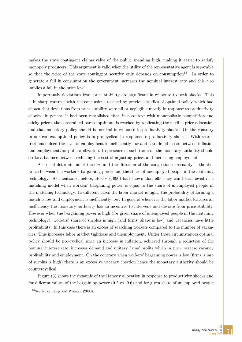
Figure (3) shows the dynamic of the Ramsey allocation in response to productivity shocks and

for different values of the bargaining power (0.2 vs. 0.6) and for given share of unemployed people

13See Khan, King and Wolman (2000).

21ECB


in the matching technology, ξ = 0.4 . When ς = 0.2 (< ξ = 0.4) optimal policy is countercyclical.

In this case there is excessive vacancy creation hence a reduction in inflation by increasing the

mark-up reduces demand and vacancy profitability. The contrary is true for ς = 0.6. In both cases

however the result is an increase in consumption, output and employment due to the reduction in

the search externality.

5.2 Comparison Between Ramsey Policy and Policy Rules

Some interesting observations come from the comparison between the dynamic under the Ramsey

policy and the dynamic generated by some simple operational policy rules. Figure (4) shows the

dynamic of selected variables in response to productivity shocks and under three different regime.

The first regime is represented by a Taylor rule of the following type:

ln

µ1 + rnt1 + rn

¶=

µφπ ln

³πtπ

´+ φy ln

µyty

¶¶(44)

with φπ = 1.5 and φy = 0.5.The second regime is represented by a rule that targets unemploy-

ment of this form:

ln

µ1 + rnt1 + rn

¶=³φπ ln

³πtπ

´+ φu ln

³utu

´´(45)

with φπ = 3 and φu = 0.3. finally the third regime is given by the Ramsey policy.

Figure (4) shows the dynamic of selected variables in response to productivity shocks and

under the three regimes described. It stands clear that the Ramsey policy implies a much higher

volatility compared to the other two rules. This is so since under both rules, the Taylor rule and the

unemployment targeting, the monetary authority is only concerned with stabilization and for this

reason behaves countercyclically (inflation goes down in response to productivity shocks). On the

contrary the Ramsey planner has the incentive to take full advantage of the productivity increase

thereby exploiting all the benefits of the expansionary phase.

5.3 Optimal Volatility of Inflation

To fully analyze the properties of the optimal policy along the cycle we are obliged to study the path

of the optimal inflation volatility for different values of the bargaining power. Once again the level

of the bargaining power is an indicator of the size and the direction of the congestion externality.

As before we expect the optimal policy to be pro-cyclical when the number of searching workers

is too high compared to the number of vacancies (e.g. when workers’ bargaining power is higher

than the share of unemployed people in the matching technology) and viceversa. However in any

case inflation volatility is increasing whenever the bargaining power gets distant from the number


of unemployed people in the matching technology. Indeed the incentive of the monetary authority

to intervene and reduce the search externality are higher when the distance between the current

employment and the efficient one increase (e.g. when the distance between workers’ bargaining

power and share of unemployed workers in the matching technology increases independently from

the direction). This is confirmed by figure (5) which shows that the optimal inflation volatility is

indeed U-shaped with respect to ς for given value of ξ = 0.4.

5.4 Adding Real Wage Rigidity

Shimer (2003), Hall (2003) noticed that in a matching model a’ la Mortensen and Pissarides wages

are too volatile since little adjustment takes place along the employment margin. They also noticed

that the introduction of real wage rigidity helps to resolve some of the puzzling features of the

standard matching model. Thereby following Hall (2003) I assume that the individual real wage is

a weighted average of the one obtained through the Nash bargaining process and the one obtained

as solution to the steady state14:

wt = λ[ς(mctzt + θtκ) + (1− ς)b] + (1− λ)w (46)

Adding real wage rigidity does not alter any of the previous results15 since it does not change

the main policy trade-offs. Optimal monetary is still characterized by significant deviations from

price stability and the optimal volatility of inflation is still a U-shaped function of the bargaining

power. The only noticeable difference is that the introduction of real wage rigidity increases the

volatility of all variables under the Ramsey policy. Intuitively real wage rigidity tends to exacerbate

the inflation/unemployment trade-off thereby calling for stronger intervention on the side of the

monetary authority. The latter result seems consistent with Blanchard and Gali’ (2005).

6 Conclusion

This paper derives optimal monetary policy in a model with monopolistic competition and sticky

prices, matching frictions and real wage rigidity in the labour market. In response to both produc-

tivity and government expenditure shocks optimal policy features significant deviations from price

stability. This is so since search externalities generate an unemployment/inflation trade-off which

induces the monetary authority to strike a balance between reducing the cost of adjusting prices

and increasing an inefficiently low employment.

14Notice that the results in this paper remain valid when the wage is set as a weighted average of current and pastvalues.15Results are not reported for brevity but are available upon request.

23ECB


In response to productivity shocks optimal policy is pro-cyclical when the worker’s bargaining

power is higher than the share of unemployed people in the matching technology and viceversa.

This is so since when the workers’ share of surplus is high (firms’ share is low) there is an excessive

number of searching workers and few vacancies. In this case the monetary authority has an incentive

to increase vacancy creation by increasing their profitability. It does that by reducing the interest

rate, therefore increasing demand and inflation. The opposite is true when the workers’ share of

surplus is low: in this case the congestion externality is generated by an excessive vacancy creation

that the monetary authority tries to discourage.


7 Appendix A - The Stationary Lagrangian Problem

Let Λnt ≡ {λ1,t, λ2,t, λ3,t, λ4,t, λ5,t}∞t=0 and Ξnt ≡ {ct, nt, vt, πt, rnt ,mct}∞t=0 to

Min{Λnt }∞t=0

Max{Ξnt }∞t=0

E0{∞Xt=0

βtEt{W (ct, nt, vt, πt,mct) (47)

+λ1,t

∙c−σt

(1 + rnt )

¸+

+λ2,t[1− ψ(πt − 1)πtytct − (1−mct)ctytε] +

+λ3,t

h κmθξtct

i+

+λ4,t

∙ntzt − κvt −

ψ

2(πt − 1)2 yt − ct − gt

¸+

+λ5,t

hnt − (1− ρ)(nt−1 + vt−1muξtv

1−ξt )

i}}

where:

W (ct, nt, vt, πt,mct) =

U(ct)− χ1,tβEt

©c−σt πt

ª+ χ2,tβEt(ct)

−σ[ψ(πt − 1)πtyt]

−χ3,tEt{β(ct)−σ(1− ρ)[(1− ς)mctzt − ςθtκ− (1− ς)b+κ

mθξt ]

θt ≡ vtutand ut = 1− nt.

25ECB


References

[1] Andolfatto, David. (1996) “Business Cycles and Labor Market Search”. American Economic

Review 86, 112-132.

[2] Andrés, Javier, David López-Salido and Javier Vallés .(2001) “Money in a Estimated Business

Cycle Model of the Euro Area”. Banco de España, WP 0121.

[3] Angeloni, Ignazio, and Luca Dedola. (1998) “From the ERM to the EMU: New Evidence on

Convergence in the Euro Area”. ECB w.p.

[4] Basu, Susanto, and John Fernald. (1997) “Returns to Scale in U.S. Production: Estimates and

Implications”. Journal of Political Economy, vol. 105-2, pages 249-83.

[5] Blanchard, Olivier, and Paul Diamond. (1991) “The Aggregate Matching Function”. NBER

Working Papers 3175.

[6] Blanchard, Olivier, and Jordi Gali’. (2005) “Real Wage Rigidities and the New Keynesian

Model”, forthcoming Journal of Money, Credit and Banking.

[7] Blanchard, Olivier, and Jordi Gali’. (2006) “A New Keynesian Model with Unemployment”,

mimeo.

[8] Canzoneri, Matthew, R. Cumby and B. Diba. (2005) “Price and Wage Inflation Targeting:

Variations on a Theme by Erceg, Henderson and Levin”. Mimeo.

[9] Christofell, Kai, and Tobias Linzert. (2005) “ The Role of Real Wage Rigidity and Labor

Market Flows for Unemployment and Inflation Dynamics”. Mimeo.

[10] Clarida, Richard, Jordi Gali, and Mark Gertler. (2000) “Monetary Policy Rules and Macro-

economic Stability: Evidence and Some Theory”. Quarterly Journal of Economics, 115 (1),

147-180.

[11] Cole, Harald L., and R. Rogerson. (1996) “Can the Mortensen-Pissarides matching model

match the business cycle facts?”. Staff Report 224, Federal Reserve Bank of Minneapolis.

[12] Cooley, Thomas and Vincenzo Quadrini. (2004) “Investment and liquidation in renegotiation-

proof contracts with moral hazard”. Journal of Monetary Economics, 51(4), 713-751.

[13] den Haan, Wouters, Gary Ramey, and James Watson. (2000) “Job Destruction and Propaga-

tion of Shocks”. American Economic Review 90, 482-498.


[14] Erceg, Christopher J., Henderson, Dale W. and Andrew T. Levin. (2000) “Optimal monetary

policy with staggered wage and price contracts”. Journal of Monetary Economics, 46(2), 281-

313.

[15] Faia, Ester. (2005) “Ramsey Monetary Policy with Capital Accumulation and Nominal Rigidi-

ties”, forthcoming in Macroeconomic Dynamics.

[16] Faia, Ester. (2005) “Optimal Monetary Policy Rules with Labor Market Frictions”, mimeo.

[17] Faia, Ester, and Tommaso Monacelli. (2005) “Optimal Monetary Policy Rules with Credit

Market Imperfections”. Forthcoming in the Journal of Economic Dynamics and Control.

[18] Hall, Robert (2003). “Wage Determination and Employment Fluctuations”. NBER W. P.

#9967.

[19] Hashimzade, Nigar, and Salvador Ortigueira. (2005) “Endogenous Business Cycles with Fric-

tional Labour Markets”. Economic Journal.

[20] Hosios, Arthur J. (1990) “On the Efficiency of Matching and Related Models of Search and

Unemployment”. Review of Economic Studies, 57(2), 279-98.

[21] Kim, J., and K.S. Kim. (2003) “Spurious Welfare Reversals in International Business Cycle

Models”. Journal of International Economics 60, 471-500.

[22] Kim, J., and Andrew Levin. (2004 “Conditional Welfare Comparisons of Monetary Policy

Rules”. Mimeo.

[23] King, Robert, and Alexander L. Wolman. (1996) “Inflation Targeting in a St. Louis Model of

the 21st Century”. NBER W. P. 5507.

[24] Kollmann, Robert. (2003a) “Monetary Policy Rules in an Interdependent World”. CEPR DP

4012.

[25] Kollmann, Robert. (2003b) “Welfare Maximizing Fiscal and Monetary Policy Rules”. Mimeo.

[26] Krause, Michael and Thomas Lubik. (2005) “The (Ir)relevance of Real Wage Rigidity in the

New Keynesian Model with Search Frictions”. forthcoming in Journal of Monetary Economics.

[27] Merz, Monika. (1995) “Search in the Labor Market and the Real Business Cycle”. Journal of

Monetary Economics 36, 269-300.

27ECB


[28] Mortensen, D. and Christopher Pissarides. (1999) “New Developments in Models of Search

in the Labor Market”. In: Orley Ashenfelter and David Card (eds.): Handbook of Labor

Economics.

[29] Krause, Michael, and Thomas Lubik. (2004) “A Note on Instability and Indeterminacy in

Search and Matching Models”. Mimeo.

[30] Nickell, Stephen, and Luca Nunziata. (2001) “Labour Market Institutions Database.”

[31] Perotti, Roberto. (2004) “Estimating the Effects of Fiscal Policy in OECD Countries”. Mimeo.

[32] Rotemberg, Julio. (1982) “Monopolistic Price Adjustment and Aggregate Output”. Review of

Economics Studies, 44, 517-531.

[33] Ramsey, F. P.. (1927) “A contribution to the Theory of Taxation”. Economic Journal, 37:47-61.

[34] Rotemberg, Julio, and Michael Woodford. (1997) “An Optimization-Based Econometric Model

for the Evaluation of Monetary Policy”. NBER Macroeconomics Annual, 12: 297-346.

[35] Schmitt-Grohe, Stephanie, and Martin Uribe. (2003) “Optimal, Simple, and Implementable

Monetary and Fiscal Rules”. Mimeo.

[36] Schmitt-Grohe, Stephanie, and Martin Uribe. (2004a) “Solving Dynamic General Equilibrium

Models Using a Second-Order Approximation to the Policy Function”. Journal of Economic

Dynamics and Control 28, 645-858.

[37] Schmitt-Grohe, Stephanie, and Martin Uribe. (2004b) “Optimal Operational Monetary Policy

in the Christiano-Eichenbaum-Evans Model of the U.S. Business Cycle ”. Mimeo.

[38] Schmitt-Grohe, Stephanie, and Martin Uribe. (2005) “Optimal Inflation Stabilization in a

Medium-Scale Macroeconomic Model”. Mimeo.

[39] Shimer, Robert. (2003) “The Cyclical Behavior of Equilibrium Unemployment and Vacancies:

Evidence and Theory”. forthcoming American Economic Review.

[40] Smets, Frank, and Raf Wouters. (2003) “An Estimated Dynamic Stochastic General Equilib-

riumModel of the Euro Area”. Journal of the European Economic Association, 1(5), 1123-1175.

[41] Walsh, Carl. (2003) “Labor Market Search and Monetary Shocks”. In: S. Altug, J. Chadha,

and C. Nolan (eds.): Elements of Dynamic Macroeconomic Analysis, Cambridge University

Press

[42] Woodford, Michael. (2003) Interest and Prices : Foundations of a Theory of Monetary Policy.


0 20 40 60−2

0

2

4Consumption

0 20 40 600

0.5

1

1.5Employment

0 20 40 60−6

−4

−2

0Unemployment

0 20 40 60−2

0

2

4Prices

0 20 40 60−2

0

2

4Inflation

0 20 40 60−2

0

2

4Output

Figure 1: Impulse responses under Ramsey allocation to productivity shocks.

29ECB


0 20 40 60−1

−0.5

0

0.5Consumption

0 20 40 60−0.5

0

0.5Employment

0 20 40 60−1

0

1

2Unemployment

0 20 40 60−1.5

−1

−0.5

0Prices

0 20 40 60−1

−0.5

0

0.5Inflation

0 20 40 60−0.5

0

0.5Output

Figure 2: Impulse responses under Ramsey allocation to government expenditure shocks.


0 10 20 30 40 50 60−1

0

1

2

3

4Consumption

0 10 20 30 40 50 60−0.5

0

0.5

1

1.5Employment

0 10 20 30 40 50 60−4

−3

−2

−1

0

1Unemployemnt

0 10 20 30 40 50 60−2

−1

0

1

2

3

4Prices

0 10 20 30 40 50 60−1

0

1

2

3Inflation

0 10 20 30 40 50 60−0.5

0

0.5

1

1.5

2

2.5Output

ETA=0.2ETA=0.6

Impulse responses of Ramsey allocation to productivity shocks under different values of bargainingpower

Figure 3:

31ECB


0 10 20 30 40 50 60−1

0

1

2

3Consumption

0 10 20 30 40 50 60−0.5

0

0.5

1

1.5Employment

0 10 20 30 40 50 60−5

−4

−3

−2

−1

0

1Unemploymnet

0 10 20 30 40 50 60−25

−20

−15

−10

−5

0

5Prices

0 10 20 30 40 50 60−2

−1

0

1

2

3Inflation

0 10 20 30 40 50 60−0.5

0

0.5

1

1.5

2

2.5Output

TaylorUnemployment targetRamsey

Impulse responses to productivity shocks under three different regimes: Taylor rules, unemployment targeting and Ramseypolicy.

Figure 4:


0.2 0.3 0.4 0.5 0.6 0.7 0.8 0.9 12

4

6

8

10

12

14

16

18Optimal inflation volatility: effect of varying bargainig power

Bargaining power

Infla

tion

vola

tility

(in

per

cent

age

devi

atio

ns)

Figure 5:

33ECB



European Central Bank Working Paper Series

For a complete list of Working Papers published by the ECB, please visit the ECB’s website(http://www.ecb.int)

680 “Comparing alternative predictors based on large-panel factor models” by A. D’Agostino and D. Giannone, October 2006.

681 “Regional inflation dynamics within and across euro area countries and a comparison with the US” by G. W. Beck, K. Hubrich and M. Marcellino, October 2006.

682 “Is reversion to PPP in euro exchange rates non-linear?” by B. Schnatz, October 2006.

683 “Financial integration of new EU Member States” by L. Cappiello, B. Gérard, A. Kadareja and S. Manganelli, October 2006.

684 “Inflation dynamics and regime shifts” by J. Lendvai, October 2006.

685 “Home bias in global bond and equity markets: the role of real exchange rate volatility” by M. Fidora, M. Fratzscher and C. Thimann, October 2006

686 “Stale information, shocks and volatility” by R. Gropp and A. Kadareja, October 2006.

687 “Credit growth in Central and Eastern Europe: new (over)shooting stars?” by B. Égert, P. Backé and T. Zumer, October 2006.

688 “Determinants of workers’ remittances: evidence from the European Neighbouring Region” by I. Schiopu and N. Siegfried, October 2006.

689 “The effect of financial development on the investment-cash flow relationship: cross-country evidence from Europe” by B. Becker and J. Sivadasan, October 2006.

690 “Optimal simple monetary policy rules and non-atomistic wage setters in a New-Keynesian framework” by S. Gnocchi, October 2006.

691 “The yield curve as a predictor and emerging economies” by A. Mehl, November 2006.

692 “Bayesian inference in cointegrated VAR models: with applications to the demand for euro area M3” by A. Warne, November 2006.

693 “Evaluating China’s integration in world trade with a gravity model based benchmark” by M. Bussière and B. Schnatz, November 2006.

694 “Optimal currency shares in international reserves: the impact of the euro and the prospects for the dollar” by E. Papaioannou, R. Portes and G. Siourounis, November 2006.

695 “Geography or skills: What explains Fed watchers’ forecast accuracy of US monetary policy?” by H. Berger, M. Ehrmann and M. Fratzscher, November 2006.

35ECB


696 “What is global excess liquidity, and does it matter?” by R. Rüffer and L. Stracca, November 2006.

697 “How wages change: micro evidence from the International Wage Flexibility Project” by W. T. Dickens, L. Götte, E. L. Groshen, S. Holden, J. Messina, M. E. Schweitzer, J. Turunen, and M. E. Ward, November 2006.

698 “Optimal monetary policy rules with labor market frictions” by E. Faia, November 2006.

699 “The behaviour of producer prices: some evidence from the French PPI micro data” by E. Gautier, December 2006.

700 “Forecasting using a large number of predictors: Is Bayesian regression a valid alternative toprincipal components?” by C. De Mol, D. Giannone and L. Reichlin, December 2006.

701 “Is there a single frontier in a single European banking market?” by J. W. B. Bos and H. Schmiedel, December 2006.

702 “Comparing financial systems: a structural analysis” by S. Champonnois, December 2006.

703 “Comovements in volatility in the euro money market” by N. Cassola and C. Morana, December 2006.

704 “Are money and consumption additively separable in the euro area? A non-parametric approach” by B. E. Jones and L. Stracca, December 2006.

705 “What does a technology shock do? A VAR analysis with model-based sign restrictions” by L. Dedola and S. Neri, December 2006.

706 “What drives investors’ behaviour in different FX market segments? A VAR-based returndecomposition analysis” by O. Castrén, C. Osbat and M. Sydow, December 2006.

707 “Ramsey monetary policy with labour market frictions” by E. Faia, January 2007.

ISSN 1561081-0

9 7 7 1 5 6 1 0 8 1 0 0 5

ramsey monetary policy with labour market frictions1

Documents