ram kit hes is

8/3/2019 Ram Kit Hes Is

http://slidepdf.com/reader/full/ram-kit-hes-is 1/45

CHAPTER 1

1. INTRODUCTION:

Uncompressed multimedia (graphics, audio and video) data requires considerable storage

capacity and transmission bandwidth. Despite rapid progress in mass-storage density, processor

speeds, and digital communication system performance, demand for data storage capacity and

data-transmission bandwidth continues to outstrip the capabilities of available technologies. The

recent growth of data intensive multimedia-based web applications have not only sustained the

need for more efficient ways to encode signals and images but have made compression of such

signals central to storage and communication technology.

Image compression can be lossy or lossless. Lossless compression involves with

compressing data which when decompressed, will be an exact replica of the original data. This is

the case when binary data such as executables, documents etc. are compressed they need to be

exactly reproduced when decompressed. On the other hand, images (and music too) need not be

reproduced exactly.

Near-lossless compression denotes compression methods, which give quantitative bounds

on the nature of the loss that is introduced. Such compression techniques provide the guarantee

that no pixel difference between the original and the compressed image is above a given value.

An approximation of the original image is enough for most purposes, as long as the error

between the original and the compressed image is tolerable. This is because lossy compression

methods, especially when used at low bit rates, introduce compression artifacts. For the lossy

reconstructions at the intermediate stages, no precise bounds can be set on the extent of distortion

present. Near-lossless compression in such a framework is only possible either by an appropriate

pre quantization of the wavelet coefficients and lossless transmission of the resulting bit stream,

or by truncation of the bit stream at an appropriate point followed by transmission of a residual

layer to provide the near-lossless bound.

This project aims on providing an application of neural networks to still image compression infrequency domains. The sparse properties of Support Vector Machine (SVM) learning are

exploited in the compression algorithms. SVM has the property that it will choose the minimum

number of training points to use as centers of the Gaussian kernel functions. It is this property

that is exploited as the basis for image compression algorithm. compression is more efficient in

frequency space.

1



1.1 OBJECTIVE:

• To clearly understand and to Implement An Algorithm for the Application of

SVM(Non Linear Regression) Learning and DCT to Image Compression

• To compare the obtained results with the standard image compression techniques

available like JPEG.

• To obtain good quality, good compression ratio and signal to noise ratio within

the required bound

2



1.2 DETAILED LITERATURE SURVEY:

IMAGE COMPRESSION

The degree of compression is best expressed in terms of the average information or entropy

of a compressed image source, expressed in terms of bits/pixel. Regardless of the particular

technique used, compression engines accomplish their intended purpose in the following manner:

1. Those portions of the image which are not perceptible to the human eye are not

transmitted.

2. Frame redundancies in the image are not transmitted.

3. The remaining information is coded in an efficient manner for transmission.

Currently, a number of image compression techniques are being used singly or in combination.

These include the following

1.2.1 ARTIFICIAL NEURAL NETWORKS[1]

In this paper describes an algorithm using backpropagation learning in a feed forward

network. The number of hidden neurons were fixed before learning and the weights of the

network after training were transmitted. The neural network (and hence the image) could then be

3



recovered from these weights. Compression was generally around 8:1 with an image quality

much lower than JPEG.

1.2.2 IMAGE COMPRESSION BY SELF-ORGANIZED KOHONEN MAP[2]

In this paper a compression scheme based on the discrete cosine transform (DCT), vector

Quantization of the DCT coefficients by Kohonen map, differential coding by first-order

predictor and entropic coding of the differences. This method gave better performance than

JPEG for compression ratios greater than 30:1

.

1.2.3 SUPPORT VECTORS IN IMAGE COMPRESSION[3]

In this paper The use of support vector machines (SVMs) in an image compression

algorithm was first presented. This method used SVM to directly model the color surface.

The parameters of a neural network (weights and Gaussian centers) were transmitted so that

the color surface could be reconstructed from a neural network using these parameters.

1.2.4 SUPPORT VECTOR REGRESSION MACHINES[4]

In this paper a new regression technique based on Vapnik’s concept of support vectors is

introduced. We compare support vector regression (SVR) with a committee regression

technique (bagging) based on regression trees and ridge regression done in feature space.

On the basis of these experiments it is expected that SVR will have advantages in high

dimensionality space because SVR optimization does not depend on the dimension &y of

the input space

1.2.5 SUPPORT VECTOR METHOD FOR FUNCTION OF APPROXIMATION[5]

In this paper The Support Vector (SV) method was recently proposed for estimating

regressions, constructing multidimensional splines, and solving linear operator equationsIn this presentation we report results of applying the SV method to these problems. 1

Introduction The Support Vector method is a universal tool for solving multidimensional

function estimation problems. Initially it was designed to solve pattern recognition

problems, where in order to find a decision rule with good generalization ability one

selects some (small) subset of the training data, called the Support Vectors (SVs).

4



Optimal separation of the SVs is equivalent to optimal separation the entire data. This led

to a new method of representing decision functions where the decision functions are a

linear expansion on a basis whose elements are nonlinear functions parameterized by the

SVs (we need one SV for each element of the basis).

1.2.6 THE NATURE OF STATISTICAL LEARNING THEORY[6]

The aim of this book is to discuss the fundamental ideas which lie behind the statistical

theory of learning and generalization. It considers learning as a general problem of

function estimation based on empirical data. These include the setting of learning

problems based on the model of minimizing the risk functional from empirical data .

a comprehensive analysis of the empirical risk minimization principle including

necessary and sufficient conditions for its consistency non-asymptotic bounds for the risk

achieved using the empirical risk minimization principles for controlling the

generalization ability of learning machines using small sample sizes based on these

bounds the Support Vector methods that control the generalization ability when

estimating function using small sample size.

1.2.7 SUPPORT VECTOR MACHINES, NEUTRAL NETWORKS AND FUZZY LOGIC

MODELS [7]

This is the first textbook that provides a thorough, comprehensive and unified

introduction to the field of learning from experimental data and soft computing. Support

vector machines (SVMs) and neural networks (NNs) are the mathematical structures, or

models, that underlie learning, while fuzzy logic systems (FLS) enable us to embed

structured human knowledge into workable algorithms. The book assumes that it is not

only useful, but necessary, to treat SVMs, NNs, and FLS as parts of a connected whole..

This approach enables the reader to develop SVMs, NNs, and FLS in addition to

understanding them.

1.2.8 IMAGE COMPRESSION WITH NEURAL NETWORKS [8]

5



In this paper new technology such as neural networks and genetic algorithms are being

developed to explore the future of image coding. Successful applications of neural

networks to vector quantization have now become well established, and other aspects of

neural network involvement in this area are stepping up to play significant roles in

assisting with those traditional technologies. This paper presents an extensive survey on

the development of neural networks for image compression which covers three

categories: direct image compression by neural networks; neural network implementation

of existing techniques, and neural network based technology which provide improvement

over traditional algorithms.

.2.9 NEURAL NETWORKS BY SIMON HAYKINS[9]

The author of this book has briefed about the concepts of SVM. How SVM is used in

pattern recognition. This book also gives the information about the generalization ability

of a linear SVM and also about the kernels used.

CHAPTER 2

BACKGROUND THEORIES

2.1 IMAGE COMPRESSION:

Image compression is the application of Data compression on digital images. In

effect, the objective is to reduce redundancy of the image data in order to be able to store or

transmit data in an efficient form. Image compression is minimizing the size in bytes of a

graphics file without degrading the quality of the image to an unacceptable level. The reduction

in file size allows more images to be stored in a given amount of disk or memory space. It also

reduces the time required for images to be sent over the Internet or downloaded from Web pages.

2.1.1 APPLICATIONS:

Currently image compression is recognized as an “Enabling Technology”. Its been used in

following applications,

6



• Image compression is the natural technology for handling the increased spatial

resolutions of today’s imaging sensors and evolving broadcast television standards.

• Plays a major role in many important and diverse applications including tele video

conferencing, remote sensing, document and medical imaging, facsimile transmission.

• Its also very useful in control of the remotely piloted vehicles in military, space and

hazardous waste management applications.

2.1.2 NEED FOR COMPRESSION:

One of the important aspects of image storage is its efficient compression. To make

this fact clear let's see an example. An image, 1024 pixel x 1024 pixel x 24 bit, without

compression, would require 3 MB of storage and 7 minutes for transmission, utilizing a high

speed, 64 Kbps, ISDN line. If the image is compressed at a 10:1 compression ratio, the storage

requirement is reduced to 300 KB and the transmission time drops to under 6 seconds. Seven 1

MB images can be compressed and transferred to a floppy disk in less time than it takes to send

one of the original files, uncompressed, over an AppleTalk network.

In a distributed environment large image files remain a major bottleneck within systems.

Compression is an important component of the solutions available for creating file sizes of

manageable and transmittable dimensions. Increasing the bandwidth is another method, but the

cost sometimes makes this a less attractive solution.At the present state of technology, the only solution is to compress multimedia data

before its storage and transmission, and decompress it at the receiver for play back. For example,

with a compression ratio of 32:1, the space, bandwidth, and transmission time requirements can

be reduced by a factor of 32, with acceptable quality.

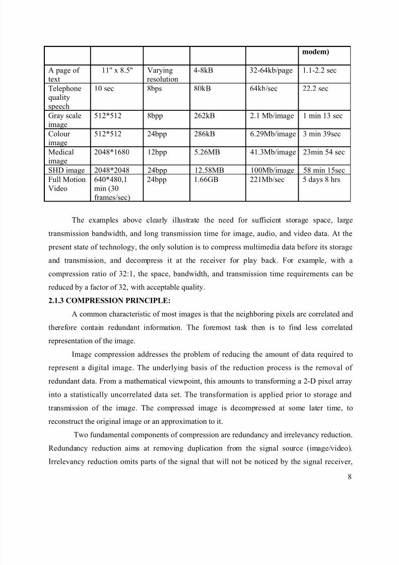
The figures in Table 1 show the qualitative transition from simple text to full-motion

video data and the disk space, transmission bandwidth, and transmission time needed to store and

transmit such uncompressed data.

Table 2.1 Multimedia data types and uncompressed storage space, transmission bandwidth, and transmission

time required. The prefix kilo- denotes a factor of 1000 rather than 1024.

Multimedi

a data

Size/Duration Bits/pixel

(or)

Bits/Sample

Uncompressed

size (B for

Bytes)

Transmission

Bandwidth

(b for bits)

Transmission

time.(using a

28.8k

7



modem)

A page of text

11'' x 8.5'' Varyingresolution

4-8kB 32-64kb/page 1.1-2.2 sec

Telephone

qualityspeech

10 sec 8bps 80kB 64kb/sec 22.2 sec

Gray scaleimage

512*512 8bpp 262kB 2.1 Mb/image 1 min 13 sec

Colour image

512*512 24bpp 286kB 6.29Mb/image 3 min 39sec

Medicalimage

2048*1680 12bpp 5.26MB 41.3Mb/image 23min 54 sec

SHD image 2048*2048 24bpp 12.58MB 100Mb/image 58 min 15sec

Full Motion

Video

640*480,1

min (30

frames/sec)

24bpp 1.66GB 221Mb/sec 5 days 8 hrs

The examples above clearly illustrate the need for sufficient storage space, large

transmission bandwidth, and long transmission time for image, audio, and video data. At the

present state of technology, the only solution is to compress multimedia data before its storage

and transmission, and decompress it at the receiver for play back. For example, with a

compression ratio of 32:1, the space, bandwidth, and transmission time requirements can be

reduced by a factor of 32, with acceptable quality.

2.1.3 COMPRESSION PRINCIPLE:

A common characteristic of most images is that the neighboring pixels are correlated and

therefore contain redundant information. The foremost task then is to find less correlated

representation of the image.

Image compression addresses the problem of reducing the amount of data required to

represent a digital image. The underlying basis of the reduction process is the removal of

redundant data. From a mathematical viewpoint, this amounts to transforming a 2-D pixel array

into a statistically uncorrelated data set. The transformation is applied prior to storage andtransmission of the image. The compressed image is decompressed at some later time, to

reconstruct the original image or an approximation to it.

Two fundamental components of compression are redundancy and irrelevancy reduction.

Redundancy reduction aims at removing duplication from the signal source (image/video).

Irrelevancy reduction omits parts of the signal that will not be noticed by the signal receiver,

8



namely the Human Visual System (HVS). In general, three types of redundancy can be

identified:

• Spatial Redundancy or correlation between neighboring pixel values.

• Spectral Redundancy or correlation between different color planes or spectral

bands.

• Temporal Redundancy or correlation between adjacent frames in a sequence of

images (in video applications).

Image compression research aims at reducing the number of bits needed to represent an

image by removing the spatial and spectral redundancies as much as possible.

The best image quality at a given bit-rate (or compression rate) is the main goal of image

compression. However, there are other important properties of image compression schemes.

Scalability generally refers to a quality reduction achieved by manipulation of the bits-stream

or file (without decompression and re-compression). Other names for scalability are progressive

coding or embedded bit-streams. Despite its contrary nature, scalability can also be found in

lossless codec’s, usually in form of coarse-to-fine pixel scans. Scalability is especially useful for

previewing images while downloading them (e.g. in a web browser) or for providing variable

quality access to e.g. databases. There are several types of scalability:

• Quality progressive or layer progressive: The bit-stream successively refines the

reconstructed image.

• Resolution progressive: First encode a lower image resolution; then encode the difference

to higher resolutions.

• Component progressive: First encode grey; then color.

Region of interest coding: Certain parts of the image are encoded with higher quality than others.

This can be combined with scalability (encode these parts first, others later).

Meta information: Compressed data can contain information about the image which can be used

to categorize, search or browse images. Such information can include color and texture statistics,

small preview images.

9



The quality of a compression method is often measured by the Peak signal-to-noise ratio.

It measures the amount of noise introduced through a lossy compression of the image. However,

the subjective judgment of the viewer is also regarded as an important, perhaps the most

important measure.

2.1.4 CLASSIFICATION OF COMPRESSION TECHNIQUE:

Two ways of classifying compression techniques are mentioned here.

(a) Lossless vs. Lossy compression:

In lossless compression schemes, the reconstructed image, after compression, is

numerically identical to the original image. However lossless compression can only to

achieve a modest amount of compression. An image reconstructed following lossy

compression contains degradation relative to the original. Often this is because the

compression scheme completely discards redundant information. However, lossy

schemes are capable of achieving much higher compression. Under normal viewing

conditions, no visible loss is perceived (visually lossless).

Compressing an image is significantly different than compressing raw binary data. Of

course, general-purpose compression programs can be used to compress images, but the

result is less than optimal. This is because images have certain statistical properties,

which can be exploited by encoders specifically designed for them. Also, some of the

finer details in the image can be sacrificed for the sake of saving a little more bandwidth

or storage space. Lossy compression methods are especially suitable for natural images

such as photos in applications where minor (sometimes imperceptible) loss of fidelity is

acceptable to achieve a substantial reduction in bit rate.

A text file or program can be compressed without the introduction of errors, but only up

to a certain extent. Lossless compression is sometimes preferred for artificial images such

as technical drawings, icons or comics. This is because lossy compression methods,

especially when used at low bit rates, introduce compression artifacts. Lossless

compression methods may also be preferred for high value content, such as medical

imagery or image scans made for archival purposes. This is called Lossless compression.

Beyond this point, errors are introduced. In text and program files, it is crucial that

compression be lossless because a single error can seriously damage the meaning of a

10



text file, or cause a program not to run. In image compression, a small loss in quality is

usually not noticeable. There is no "critical point" up to which compression works

perfectly, but beyond which it becomes impossible. When there is some tolerance for

loss, the compression factor can be greater than it can when there is no loss tolerance. For

this reason, graphic images can be compressed more than text files or program.

The information loss in lossy coding comes from quantization of the data. Quantization

can be described as the process of sorting the data into different bits and representing

each bit with a value. The value selected to represent a bit is called the reconstruction

value. Every item in a bit has the same reconstruction value, which leads to information

loss (unless the quantization is so fine that every item gets its own bit).

(b) Predictive vs. Transform coding: In predictive coding, information already sent or

available is used to predict future values, and the difference is coded. Since this is

done in the image or spatial domain, it is relatively simple to implement and is

readily adapted to local image characteristics. Differential Pulse Code Modulation

(DPCM) is one particular example of predictive coding. Transform coding, on the

other hand, first transforms the image from its spatial domain representation to a

different type of representation using some well-known transform and then codes the

transformed values (coefficients). This method provides greater data compression

compared to predictive methods, although at the expense of greater computation

2.1.5 IMAGE COMPRESSION MODEL:

The block diagram of the image compression model is given in fig 2.1

Figure 2.1 Image Compression Model

2.1.5.1 SOURCE ENCODER:

11

SOURCEENCODER

CHANNELENCODER

CHANNEL CHANNEL

DECODER

SOURCEDECODER



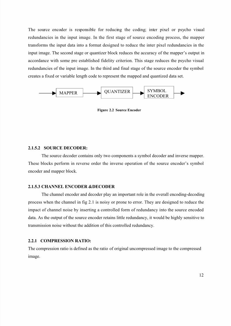
The source encoder is responsible for reducing the coding; inter pixel or psycho visual

redundancies in the input image. In the first stage of source encoding process, the mapper

transforms the input data into a format designed to reduce the inter pixel redundancies in the

input image. The second stage or quantizer block reduces the accuracy of the mapper’s output in

accordance with some pre established fidelity criterion. This stage reduces the psycho visual

redundancies of the input image. In the third and final stage of the source encoder the symbol

creates a fixed or variable length code to represent the mapped and quantized data set.

Figure 2.2 Source Encoder

2.1.5.2 SOURCE DECODER:

The source decoder contains only two components a symbol decoder and inverse mapper.

These blocks perform in reverse order the inverse operation of the source encoder’s symbol

encoder and mapper block.

2.1.5.3 CHANNEL ENCODER &DECODER

The channel encoder and decoder play an important role in the overall encoding-decoding

process when the channel in fig 2.1 is noisy or prone to error. They are designed to reduce the

impact of channel noise by inserting a controlled form of redundancy into the source encoded

data. As the output of the source encoder retains little redundancy, it would be highly sensitive to

transmission noise without the addition of this controlled redundancy.

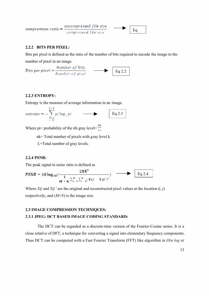
2.2.1 COMPRESSION RATIO:

The compression ratio is defined as the ratio of original uncompressed image to the compressed

image.

12

MAPPER QUANTIZER SYMBOL

ENCODER



2.2.2 BITS PER PIXEL:

Bits per pixel is defined as the ratio of the number of bits required to encode the image to the

number of pixel in an image.

2.2.3 ENTROPY:

Entropy is the measure of average information in an image.

Where pi= probability of the ith gray level=

nk= Total number of pixels with gray level k

L=Total number of gray levels.

2.2.4 PSNR:

The peak signal to noise ratio is defined as

Where Xij and Xij ′ are the original and reconstructed pixel values at the location (i, j)

respectively, and (M × N ) is the image size.

2.3 IMAGE COMPRESSION TECHNIQUES:

2.3.1 JPEG: DCT BASED IMAGE CODING STANDARD:

The DCT can be regarded as a discrete-time version of the Fourier-Cosine series. It is a

close relative of DFT, a technique for converting a signal into elementary frequency components.

Thus DCT can be computed with a Fast Fourier Transform (FFT) like algorithm in O(n log n)

13

Eq

Eq 2.4

Eq 2.3

Eq 2.2



operations. Unlike DFT, DCT is real-valued and provides a better approximation of a signal with

fewer coefficients. The DCT of a discrete signal x(n), n=0, 1, .. , N-1 is defined as:

where, α(u) = 0.707 for u = 0 and

= 1 otherwise.

JPEG established the first international standard for still image compression where the encoders

and decoders are DCT-based. The JPEG standard specifies three modes namely sequential,

progressive, and hierarchical for lossy encoding, and one mode of lossless encoding. The

`baseline JPEG coder' which is the sequential encoding in its simplest form, will be briefly

discussed here. Fig. 2.3 and 2.4 show the key processing steps in such an encoder and decoder

for grayscale images. Color image compression can be approximately regarded as compression

of multiple grayscale images, which are either compressed entirely one at a time, or are

compressed by alternately interleaving 8x8 sample blocks from each in turn.

The original image block is recovered from the DCT coefficients by applying the inverse discrete

cosine transform (IDCT), given by:

Where, α(u) = 0.707 for u = 0 and

= 1 otherwise.

Steps in JPEG Compression:

1. If the color is represented in RGB mode, translate it to YUV.

2. Divide the file into 8 X 8 blocks.

14

Eq 2.5

Eq 2.6



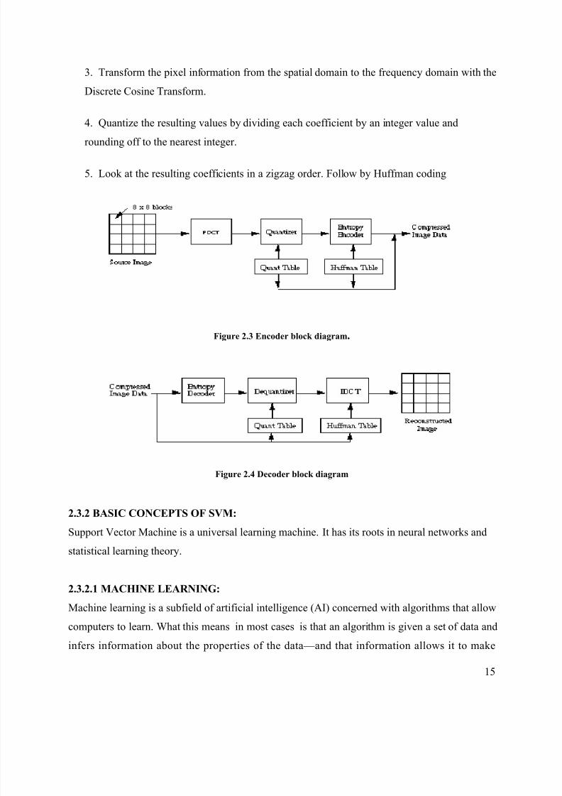
3. Transform the pixel information from the spatial domain to the frequency domain with the

Discrete Cosine Transform.

4. Quantize the resulting values by dividing each coefficient by an integer value and

rounding off to the nearest integer.

5. Look at the resulting coefficients in a zigzag order. Follow by Huffman coding

Figure 2.3 Encoder block diagram.

Figure 2.4 Decoder block diagram

2.3.2 BASIC CONCEPTS OF SVM:

Support Vector Machine is a universal learning machine. It has its roots in neural networks and

statistical learning theory.

2.3.2.1 MACHINE LEARNING:

Machine learning is a subfield of artificial intelligence (AI) concerned with algorithms that allow

computers to learn. What this means in most cases is that an algorithm is given a set of data and

infers information about the properties of the data—and that information allows it to make

15



predictions about other data that it might see in the future. This is possible because almost all

nonrandom data contains patterns, and these patterns allow the machine to generalize. In order to

generalize, it trains a model with what it determines are the important aspects of the data.

To understand how models come to be, we consider a simple example in the otherwise complex

field of email filtering. Suppose we receive a lot of spam that contains the words online

pharmacy. As a human being, we are well equipped to recognize patterns, and can quickly

determine that any message with the words online pharmacy is spam and should be moved

directly to the trash. This is a generalization we have in fact created a mental model of what is

spam.

There are many different machine-learning algorithms, all with different strengths and suited to

different types of problems. Some, such as decision trees, are transparent, so that an observer can

totally understand the reasoning process undertaken by the machine. Others, such as neural

networks, are black box meaning that they produce an answer, but it‘s often very difficult to

reproduce the reasoning behind it

2.3.2.2 SUPPORT VECTOR MACHINE:

Support vector machines (SVM), introduced by Vapnik and coworkers in 1992, and has been

noted as one of the best classifiers during the past 20 years. It is popular in bioinformatics, text

analysis and pattern classification. As a learning method support vector machine is regarded as

one of the best classifiers with a strong mathematical foundation. During the past decade, SVM

has been commonly used as a classifier for various applications

The handling of high feature dimensionality and the labeling of training data are the two major

challenges in pattern recognition. To handle the high feature dimensionality, there are two major

approaches. One is to use special classifiers which are not sensitive to dimensionality, for

example, SVM algorithm.

2.3.2.3 LINEAR CLASSIFICATION PROBLEM:

Most matrimonial sites collect a lot of interesting information about their members, including

demographic information, interests, and behavior. Imagine that this site collects the following

information:

16



• Age

• List of interests

• Location

• Qualification

Furthermore, this site collects information about whether two people have made a good match,

whether they initially made contact, and if they decided to meet in person. This data is used to

create the matchmaker dataset.

Each row has information about a man and a woman and, in the final column, a 1or a 0 to

indicate whether or not they are considered a good match. For a site with a large number of

profiles, this information might be used to build a predictive algorithm that assists users in

finding other people who are likely to be good matches. It might also indicate particular types of

people that the site is lacking, which would be useful in strategies for promoting the site to new

members. Lets take only the parameter ages and give the match information to illustrate how the

classifiers work, since two variables are much easier to visualize.

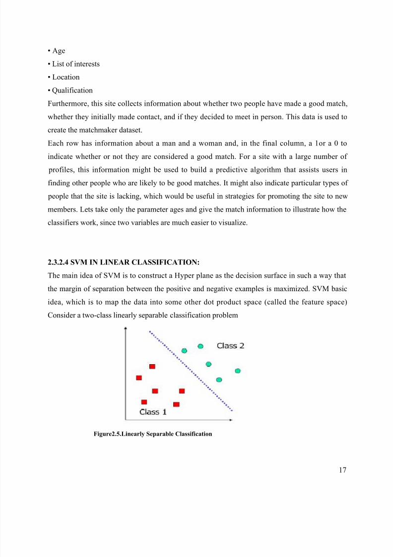
2.3.2.4 SVM IN LINEAR CLASSIFICATION:

The main idea of SVM is to construct a Hyper plane as the decision surface in such a way that

the margin of separation between the positive and negative examples is maximized. SVM basic

idea, which is to map the data into some other dot product space (called the feature space)

Consider a two-class linearly separable classification problem

Figure2.5.Linearly Separable Classification

17



Let { x1, ..., xn} be our data set and let di= {1,-1} be the class label of xi .The decision boundary

should classify all points correctly. The decision boundary is the Hyperplane. The equation of the

Hyperplane is given by WT.X+b=0

Where x is the input vector and w is the adjustable weight vector, b is the bias. The problem here

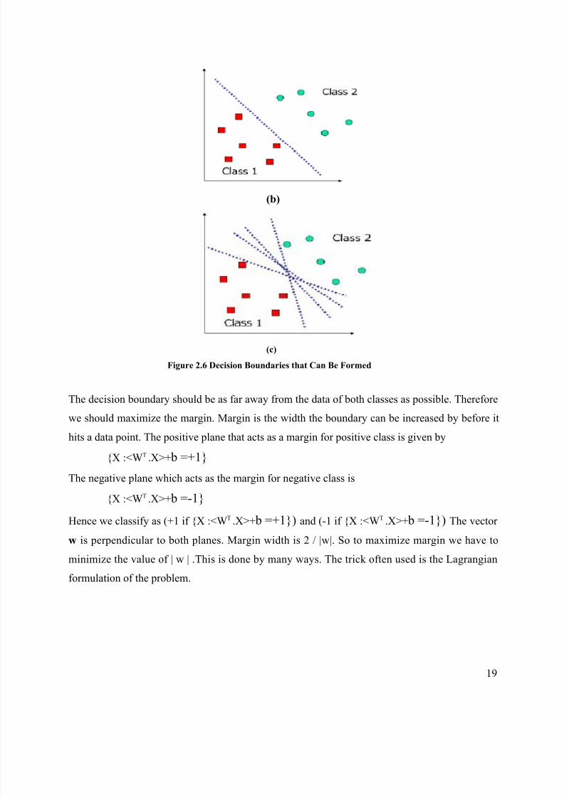
is there can be many decision boundaries as shown in figure 2.6 (a), 2.6(b) and 2.7(c)

(a)

18



(b)

(c)

Figure 2.6 Decision Boundaries that Can Be Formed

The decision boundary should be as far away from the data of both classes as possible. Therefore

we should maximize the margin. Margin is the width the boundary can be increased by before it

hits a data point. The positive plane that acts as a margin for positive class is given by

{X :<WT .X>+ b =+1}

The negative plane which acts as the margin for negative class is

{X :<WT .X>+ b =-1}

Hence we classify as (+1 if {X :<WT .X>+ b =+1}) and (-1 if {X :<WT .X>+ b =-1}) The vector

w is perpendicular to both planes. Margin width is 2 / |w|. So to maximize margin we have to

minimize the value of | w | .This is done by many ways. The trick often used is the Lagrangian

formulation of the problem.

19



Figure 2.7 Support Vectors and the Hyperplane

Support Vectors are those points which the margin pushes up against the Hyperplane. The

particular data points for which the following equations is satisfied with the equality sign are

called the support vectors, hence the name support vector machine. These vectors play a

prominent role in the operation of this class of learning machine. In conceptual terms the support

vectors are those points that lie closest to the Hyperplane are the most difficult to classify. As

such they have the direct bearing on the optimum location of the decision surface.

2.3.2.5 SOLUTION BY LAGRANGIAN MULTIPLIERS:

The Lagrangian is written:

]1) bxw(y[ww5.0), b,w(L i

Tl

1i

ii

T −+α−=α ∑=

where the αi are the Lagrange multipliers. This is now an optimization problem without

constraints where the objective is to minimize the Lagrangian L (w,b,α).

2.3.2.6 NON-SEPARABLE CLASSIFICATION:

There is no line that can be drawn between the two classes that separates the data without

misclassifying some data points. Now the aim is to find the hyperplane that makes the smallest

number of errors. Non-negative ‘slack’ variables ξ1, ξ2, ξ3,… ξl are introduced. These measure the

20



deviation of the data from the maximal margin, thus it is desirable that the ξi be as small as

possible.

The optimization problem is now:

∑= ξ+=

l

1ii

2

C||w||5.0)w,x(f

Here C is a design parameter called the penalty parameter. The penalty parameter controls the

magnitude of the ξi An increase in C penalizes larger errors (large ξi ). However this can be

achieved only by increasing the weight vector norm W (that we want to minimize). At the same

time an increase in W does not guarantee smaller ξi

Figure2.8. Non Linearly Separable Classification

2.3.2.7 Function Approximation by SVM:

Regression is an extension of the non-separable classification such that each data point can be

thought of as being in its own class.

We are now approximating functions of the form

)x(w)w,x(f i

N

1i

iφ=∑=

where the functions )x(iφ are termed kernel functions(basis functions) and N is the number of

support vectors.

Vapnik’s linear loss functions with ε-insensitivity zone as a measure of the error of

approximation:

21



Thus, the loss is equal to 0 if the difference between the predicted f (x;w) and the measured value

is less than ε. Vapnik’s ε -insensitivity loss function defines an ε tube such that if the predicted

value is within the tube the error is zero. For all other predicted points outside the tube, the error

equals the magnitude of the difference between the predicted value and the radius ε of the tube.

Error=y- f (x,w)

The total ‘risk’ or error is given by:

ε

=

−−= ∑ | bxwy|*L/1R i

Tl

1i

iemp

Now The goal is now to minimize R from the definition of (ξ i,ξi*) for data outside the

insensitivity tube ε:

|y- f(x,w)|-ε=ξ for data above ε tube

|y- f(x,w)|+ε=ξ* for data below ε tube

so our optimization problem is now to find w which minimizes the ‘risk’ or error given by

)(Cw5.0R

l

1i

*

i

l

1ii

2

,,w *

∑∑ ==ξξ ξ+ξ+=

Where ξi and ξi* are slack variables for measurements ‘above’ and ‘below’ an ε-tube respectively

and x is a Gaussian kernel. Forming the Lagrangian and finding out partial derivative w.r.to w:

i

l

1i

ii x)(w ∑=

∗α−α=

Similarly finding partial derivative w.r.to b, ξi, ξi*

We obtain matrix notation in the form of Min α−αα=α

TTf H5.0)(L

Where ]1xx[H T +=

22



T

l

2

1

l

2

1

y

...

yy

y

...

y

y

f

+ε

+ε+ε

−ε

−ε

−ε

=

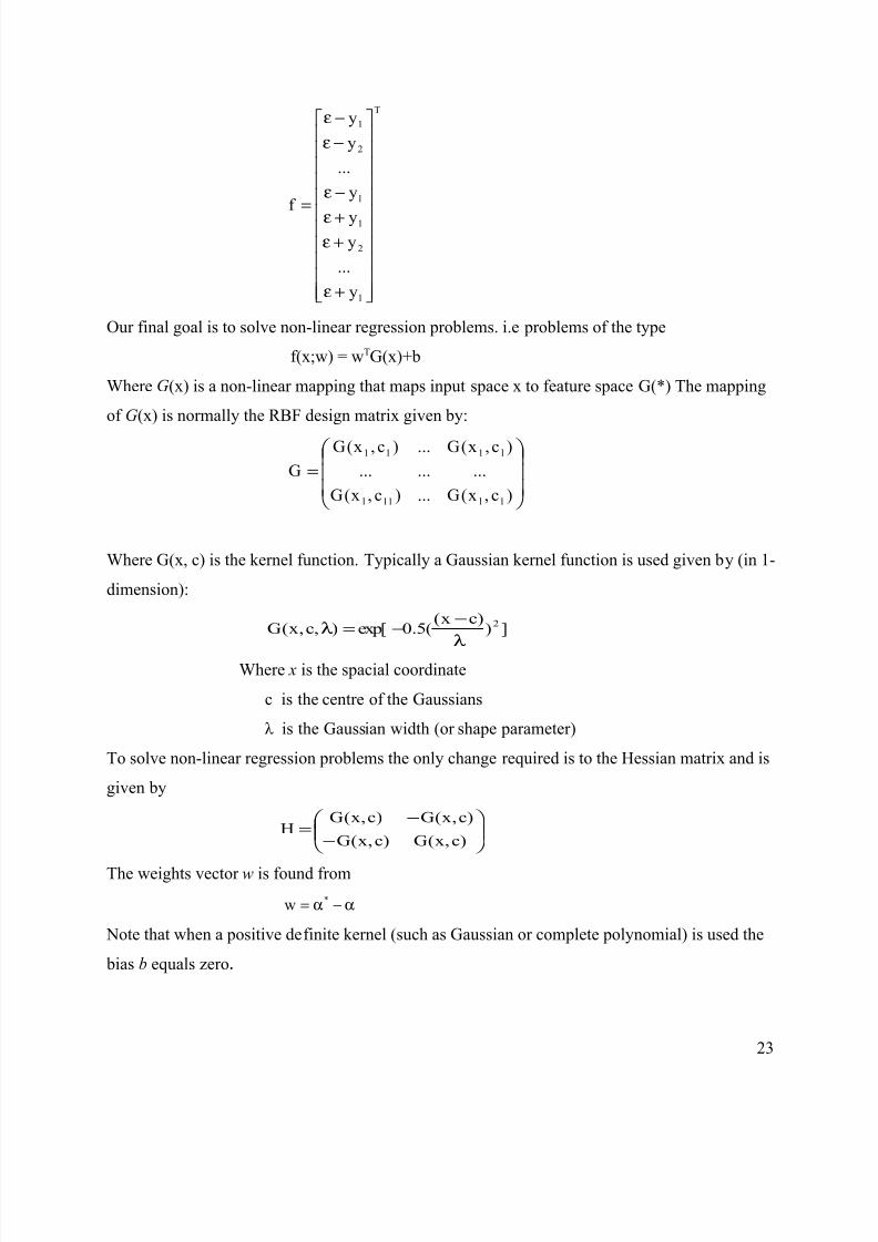
Our final goal is to solve non-linear regression problems. i.e problems of the type

f(x;w) = wTG(x)+b

Where G(x) is a non-linear mapping that maps input space x to feature space G(*) The mapping

of G(x) is normally the RBF design matrix given by:

=

)c,x(G...)c,x(G

.........

)c,x(G...)c,x(G

G

1l11l

l111

Where G(x, c) is the kernel function. Typically a Gaussian kernel function is used given by (in 1-

dimension):

]))cx(

(5.0exp[),c,x(G2

λ−

−=λ

Where x is the spacial coordinate

c is the centre of the Gaussians

λ is the Gaussian width (or shape parameter)

To solve non-linear regression problems the only change required is to the Hessian matrix and is

given by

−

−=

)c,x(G)c,x(G

)c,x(G)c,x(GH

The weights vector w is found from

α−α=*w

Note that when a positive definite kernel (such as Gaussian or complete polynomial) is used the

bias b equals zero.

23



2.3.2.8 APPLICATIONS OF SUPPORT VECTOR MACHINES

Since support-vector machines work well with high-dimensional datasets, they are most often

applied to data-intensive scientific problems and other problems that deal with very complex sets

of data. Some examples include:

• Classifying facial expressions

• Detecting intruders using military datasets

• Predicting the structure of proteins from their sequences

• Handwriting recognition

• Determining the potential for damage during earthquakes

• Digital watermarking

• Image compression

CHAPTER 3

3.1 PROGRAMMING METHODOLOGY:

24



Most image compression algorithms operate in the frequency domain. That is, the image is first

processed through some frequency analyzing function, further processing is applied onto the

resulting coefficients and the results generally encoded using an entropy encoding scheme such

as Huffman coding. The JPEG image compression algorithm is an example of an algorithm of

this type. The first step of the JPEG algorithm is to subdivide the image into 8×8 blocks then

apply the DCT to each block. Next quantization is applied to the resulting DCT coefficients. This

is simply dividing each element in the matrix of DCT coefficients by a corresponding element in

a ‘quantizing matrix’. The effect of reduces the value of most coefficients, some of which vanish

(i.e. their value becomes zero) when rounding is applied. Huffman coding is used to encode the

coefficients.

In this chapter the image is transformed into the frequency domain and applies SVM to the

frequency components. The Discrete Cosine Transform (DCT) is used as it has properties which

are exploited in SVM learning. The basic idea is to transform the image using the DCT, use

SVM learning to compress the DCT coefficients and use Huffman coding to encode the data as a

stream of bits

The algorithm presented here uses the discrete cosine transform. The DCT has properties which

make it suitable to SVM learning. SVM learning is applied to the DCT coefficients. Before the

SVM learning is applied the DCT coefficients are ‘processed’ in such a way as to make the trend

of the DCT curve more suitable to generalization by a SVM.As the DCT is fundamental to the

algorithm a detailed description follows

3.2 DESCRIPTIONS:

3.2.1 Input image:

The input image that is chosen is required to be a gray scale image with intensity levels 0-255.

The input image chosen depends upon the application where the compression is required

3.2.2 DISCRETE COSINE TRANSFORM:

25



The DCT has properties making it the choice for a number of compression schemes. It is the

basis for the JPEG compression scheme The DCT is a transform that maps a block of pixel color

values in the spatial domain to values in the frequency domain.

The DCT of a discrete signal x(n), n=0, 1, .. , N-1 is defined as:


= 1 otherwise.

The DCT is more efficient on smaller images. When the DCT is applied to large images, the

rounding effects when floating point numbers are stored in a computer system result in the DCT

coefficients being stored with insufficient accuracy. The result is deterioration in image quality.

As the size of the image is increased, the number of computations increases disproportionately.

image is subdivided into 8×8 blocks. Where an image is not an integral number of 8×8 blocks,

the image can be padded with white pixels (i.e. extra pixels are added so that the image can be

divided into an integral number of 8× 8 blocks. The 2-dimensional DCT is applied to each block

so that an 8×8 matrix of DCT coefficients is produced for each block. This is termed the ‘DCT

Matrix’. The top left component of the DCT matrix is termed the ‘DC’ coefficient and can be

interpreted as the component responsible for the average background colour of the block.The

remaining 63 components of the DCT matrix are termed the ‘AC’ components as they are

frequency components The DC coefficient is often much higher in magnitude than the AC

components in the DCT matrix The original image block is recovered from the DCT coefficients

by applying the inverse discrete cosine transform (IDCT), given by:


= 1 otherwise

3.2.3 TRANSFORMATION OF THE DCT MATRIX TO 1-D(ZIG-ZAG

TRANSFORMATION):

26

Eq 3.1

Eq 3.2



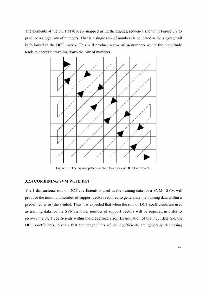
The elements of the DCT Matrix are mapped using the zig-zag sequence shown in Figure 6.2 to

produce a single row of numbers. That is a single row of numbers is collected as the zig-zag trail

is followed in the DCT matrix. This will produce a row of 64 numbers where the magnitude

tends to decrease traveling down the row of numbers.

Figure 3.1: The zig-zag pattern applied to a block of DCT Coefficients

3.2.4 COMBINING SVM WITH DCT

The 1-dimensional row of DCT coefficients is used as the training data for a SVM. SVM will

produce the minimum number of support vectors required to generalize the training data within a

predefined error (the ε-tube). Thus it is expected that when the row of DCT coefficients are used

as training data for the SVM, a lower number of support vectors will be required in order to

recover the DCT coefficients within the predefined error. Examination of the input data (i.e. the

DCT coefficients) reveals that the magnitudes of the coefficients are generally decreasing

27



traveling down the row of input data, however the sign (positive or negative) appears to be

random. This has the consequence that two coefficients next to each other can be of similar

magnitude but opposite sign causing a large swing in the input data. If the sign of each DCT

coefficient is ignored when used as input data to the SVM, there is the problem of how to re-

assign the signs when the DCT coefficients have been recovered.

The SVM learning process selects the minimum number of training points to use as the centers

of the Gaussian kernel functions in an RBF network in order for the function to be approximated

within the insensitivity zone. These selected training points are the support vectors. The

insensitivity zone drawn around the resulting function. When the penalty parameter C is infinite

the support vectors will always lie at the edge of the zone. There are only three parameters which

affect the compression which must be defined before learning can begin. These are the maximum

allowed error ε termed the insensitivity zone in SVM terminology, the penalty parameter C

and the Gaussian shape parameter.

3.2.4.1 QUADRATIC PROGRAMMING

Quadratic Programming deals with functions in which the xi are raised to the power of 0, 1, or 2.

The goal of Quadratic Programming is to determine the xi for which the function L(α) is a

minimum. The system is usually stated in Matrix and vector form.

A Quadratic program is an optimization problem with a Quadratic Objective and linear con-

straints

Minimize L(α) = (1/2) αT H α + f T α

Subject to A*x<=b

Which is usually further defined by a number of constraints (The 1/2 factor is included in the

quadratic term to avoid the appearance of a factor of 2 in the derivatives). L(α) is called the

objective function, H is a symmetric matrix called the Hessian matrix and f is a vector of

constants. This is a constrained minimization problem with quadratic function and linear

inequality constraints Where

−

−=

)c,x(G)c,x(G

)c,x(G)c,x(GH

28



and G(x) is given by the Gaussian kernel function

T

l

2

1

l

2

1

y

...

y

y

y...

y

y

f

+ε

+ε

+ε

−ε

−ε

−ε

=

3.2.4.2 KERNEL FUNCTION

The relationship between the kernel function K and the mapping φ(.) is

K(x,y)=<φ(x),φ(y)>

This is known as the kernel trick In practice, we specify K thereby specifying φ(.) indirectly

instead of choosing φ(.) Intuitively, K(x,y) represents our desired notion of similarity between

data x and y and this is from our prior knowledge K(x,y) needs to satisfy a technical condition

(Mercer condition) in order for φ(.) to exist

Linear operation in the feature space is equivalent to non-linear operation in input space

The classification task can be “easier” with a proper transformation

Transform xi to a higher dimensional space is to

– Input space: the space containing xi

– Feature space: the space of φ(xi) after transformation

Figure 3.2: Transformation of input space to future space

Gaussian kernel function is used given by (in 1-dimension):

29



]))cx(

(5.0exp[),c,x(G2

λ−

−=λ

Where

x is the spacial coordinatec is the centre of the Gaussians

λ is the Gaussian width (or shape parameter)

3.2.5 THE ‘INVERSION’ BIT

The ‘inversion bit’ indicates which of the recovered points should be inverted (i.e. multiplied by

-1) so that they are negative – that is positive points in Figure 6.4 (b) that were originally

negative are made negative by multiplying by -1 if the inversion bit is set. The inversion bit is a

single ‘0’ or ’1’. It is the sign of the corresponding input data. Each input data has an inversion bit

After a block has been processed by the SVM, some the recovered DCT coefficients may have a

magnitude lower than the maximum error defined for the SVM. If these components had an

inversion bit of ‘1’ this can be set to ‘0’ as the sign of coefficients with small magnitude does not

affect the final recovered image. Put another way, inversion bits for very small magnitude DCT

coefficients do not contain significant information required for the recovery of the image.

3.2.6 ENCODING DATA FOR STORAGE

For each block weights and support vectors are required to be stored. The support vectors are the

Gaussian centers. In our algorithm we combine the weights with the support vectors so that each

block has the same number of weights as DCT coefficients. Where a weight has no

corresponding support vector the value of the weight is set to zero. That is the only non-zero

weights are weights for which a training point has been chosen to be a support vector by the

support vector machine. The next step is to quantize the weights.

3.2.6.1 QUANTIZATION

Quantizing involves reassigning the value of the weight to one of limited number of values. To

quantize the weights the maximum and minimum weight values (for the whole image) are found

30



and the number of quantization levels are pre-defined. The number of quantization levels chosen

is a degree of freedom in the algorithm.

The steps taken to quantize the weights are:

1. Find the maximum and minimum weight values. Call these max and min.

2. Find the difference (d) between quantization levels by d=max-min/n where n is the number of

quantization levels.

3. Set lowest quantization level q1= min.

4. Set remaining quantization levels by qm=qm-1+d, until qn = max.

5. Reassign each weight the value of the closest matching quantization level qm

The inversion bits are now combined with the weights as follows. After quantization,the minimum quantization level is subtracted from each weight. This will ensure that all weights

have a positive value. An arbitrary number is added to all weights (the same number is added to

all numbers) making all weights positive and non-zero. To recover the weights both the

minimum quantization level and the arbitrary number must be stored. Each individual weight has

an associated inversion bit. The inversion bit is combined with its corresponding weight to

making the value of the weight negative if the inversion bit is ‘1’, otherwise it is positive. Where

the weight is not a support vector the inversion data is discarded. This introduces a small error

when the image is decompressed, but significantly increases compression. The above steps

introduce many ‘zero’ values into the weight data. By setting inversion bits from ‘1’ to ‘0’ when

the associated DCT is less than the error ε many more zeros are introduced.

3.2.6.2 HUFFMAN ENCODING

The quantized weights are encoded using a Huffman encoding. Huffman coding is an entropy

encoding algorithm used for lossless data compression. it is a variable length code table for

encoding a source symbol

31

http://en.wikipedia.org/wiki/Entropy_encoding


http://en.wikipedia.org/wiki/Algorithm



http://en.wikipedia.org/wiki/Algorithm



CHAPTER 4

4.1 FORMULATION OF THE APPROACH:

The image is first sub-divided into 8×8 blocks. The 2-dimensional DCT is applied to each block

to produce a matrix of DCT coefficients. The zig-zag mapping is applied to each matrix of DCT

coefficients to obtain a single row of numbers for each original block of pixels. The first term of

each row (the DC component) is separated so that only the AC terms are left. Not all the terms in

the row of AC coefficients are needed since the higher order terms do not contribute significantly

to the image. Exactly how many values are taken is a degree of freedom in the algorithm.

Support vector machine learning is applied to the absolute values of each row of AC terms as

described above and the inversion number for each block is generated. By following this method,

for each original block the Gaussian centers (i.e. the support vectors), the weights and the

inversion number need to stored/transmitted to be able to recover the block. The AC components

are used as training data to a SVM. The SVM learning process selects the minimum number of

training points to use as the centers of the Gaussian kernel functions in an RBF network in order

for the function to be approximated within the insensitivity zone. These selected training points

are the support vectors. A SVM trained on the data above with an error and Gaussian width set

to different values. The SVM was implemented in Matlab with a quadratic programming. This

will return a value for α from which we can compute the weights. In order to recover the image

the DC coefficient, the support vectors, the weights and the inversion number are stored. The

next step is to quantize the weights. Quantizing involves reassigning the value of the weight to

one of limited number of values. To quantize the weights the maximum and minimum weight

values (for the whole image) are found and the number of quantization levels are pre-defined.

The number of quantization levels chosen is a degree of freedom in the algorithm. The inversion

bits are now combined with the weights. After quantization, the minimum quantization level is

subtracted from each weight. This will ensure that all weights have a positive value. An arbitrary

number is added to all weights (the same number is added to all numbers) making all weights

positive and non-zero. To recover the weights both the minimum quantization level and the

arbitrary number must be stored. The quantized weights and number of zeros between non zero

weights are Huffman encoded to produce a binary file. The compression of the SVM surface

modeled images was computed from an actual binary file containing all information necessary

32



to recover an approximated version of the original image. To objectively measure image quality,

the signal to noise ratio (SNR) is calculated.

4.2 FLOW CHART:

33



CHAPTER 5

RESULTS AND ANALYSIS:

In this section simulation results of the performance of image algorithm is being presented and

the results are being compared with the existing JPEG algorithm. In the implementation of

Algorithm for Application of SVM(Regression) Learning and DCT to Image Compression, we

first sub-divide image into 8×8 blocks. The 2-dimensional DCT is applied to each block to

produce a matrix of DCT coefficients. The zig-zag mapping is applied to each matrix of DCT

coefficients to obtain a single row of numbers for each original block of pixels. The first term of

each row (the DC component) is separated so that only the AC terms are left. Not all the terms in

the row of AC coefficients are needed since the higher order terms do not contribute significantly

to the image. Exactly how many values are taken is a degree of freedom in the algorithm.

Support vector machine learning is applied to the absolute values of each row of AC terms as

described above and the inversion number for each block is generated. By following this method,

for each original block the Gaussian centers (i.e. the support vectors), the weights and the

inversion number need to stored/transmitted to be able to recover the block. The AC components

are used as training data to a SVM. The support vector machine learning used is identical to the

This is a constrained minimization problem with quadratic function and linear inequality

constraints. It is called quadratic programming. This will return a value for α from which we can

compute the weights. In order to recover the image the DC coefficient, the support vectors, the

weights and the inversion number are stored. The next step is to quantize the weights. Quantizing

involves reassigning the value of the weight to one of limited number of values. To quantize the

weights the maximum and minimum weight values (for the whole image) are found and the

number of quantization levels are pre-defined. The number of quantization levels chosen is a

degree of freedom in the algorithm. The inversion bits are now combined with the weights. After

quantization, the minimum quantization level is subtracted from each weight. This will ensure

that all weights have a positive value. An arbitrary number is added to all weights (the samenumber is added to all numbers) making all weights positive and non-zero. To recover the

weights both the minimum quantization level and the arbitrary number must be stored. The

quantized weights and number of zeros between non zero weights are Huffman encoded to

produce a binary file. The compression of the SVM surface modeled images was computed from

an actual binary file containing all information necessary to recover an approximated version of

34



the original image. To objectively measure image quality, the signal to noise ratio (SNR) is

calculated.

5.1 INPUT IMAGE:

Figure 5.1 Input image (a) Lena of size 128*128 is considered for compression

5.2 RESULTS OBTAINED FOR IMAGE COMPRESSION:

5.2.2 DIFFERENT VALUES OF EPSILON:

5.2.2.1 EPSILON=0.001

The image compression is obtained which can be seen in figures 5.2(e) and input image, plot of

DCT coefficients(for one example block) and plot of Absolute value of DCT coefficients, error

between the output and Desired input(for one example block) was shown in 5.2(a),

5.2(b),5.2(c),5.2(d)

35



(a) (b) (c)

(d) (e)

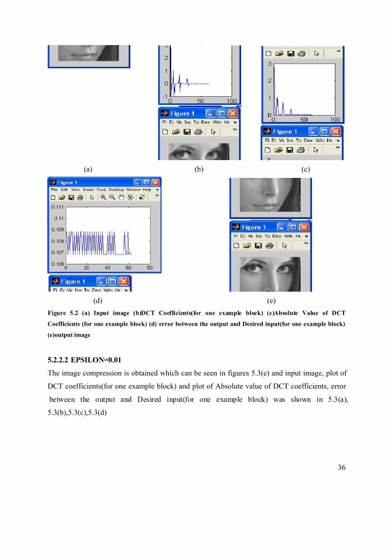
Figure 5.2 (a) Input image (b)DCT Coefficients(for one example block) (c)Absolute Value of DCT

Coefficients (for one example block) (d) error between the output and Desired input(for one example block)

(e)output image

5.2.2.2 EPSILON=0.01


DCT coefficients(for one example block) and plot of Absolute value of DCT coefficients, error between the output and Desired input(for one example block) was shown in 5.3(a),

5.3(b),5.3(c),5.3(d)

36



(a) (b) (c)

(d) (e)


Coefficients(for one example block) (d) error between the output and Desired input(for one example block)

(e)output image

5.2.2.3 EPSILON=0.1


DCT coefficients(for one example block) and plot of Absolute value of DCT coefficients, error

between the output and Desired input(for one example block) was shown in 5.4(a),

5.4(b),5.4(c),5.4(d)

37



(a) (b) (c)

(d) (e)


Coefficients(for one example block) (d) error between the output and Desired input(for one example block)

(e)output image

38



Table 5.1The number of bits with different Epsilon values, Quantization levels and number of supported

vectors respectively with Compression Ratio and SNR (DB).

5.3 COMPARISON OF THE OBTAINED RESULTS WITH JPEG ALGORITHM:

Analysis:

For the purpose o comparison of the proposed algorithm and the JPEG algorithm we have the

compression ratio for both the images. Since the bound can be set previously before in our

proposed algorithm we set the bound to be different values and we can see that the compressed

images are being compared. But in JPEG it is found to be having lots of error even though the

picture quality is being maintained. The signal to noise ratio was considered for comparison and

the value is found in db as per the formula discussed in chapter 2. It is seen that the signal to

noise ratio is very high in case of our algorithm and hence the image with the information is

highly secured and we can obtain till image compression through this algorithm

39

Different

values of

epsilon(ε)

No of

Quantizatio

n Levels

Number

of

SupportedVectors

Length

Of

HuffmanCode

Total

Numbe

r of Bits

Compressio

n Ratio

SN

R(D

B)

0.001 60 16128 64343 131072 2.03 38

0.01 60 16128 36107 131072 3.63 22

0.1 60 8756 22354 131072 5.86 18



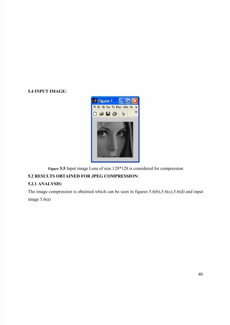
5.4 INPUT IMAGE:

Figure 5.5 Input image Lena of size 128*128 is considered for compression

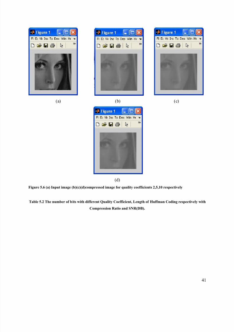
5.2 RESULTS OBTAINED FOR JPEG COMPRESSION:

5.2.1 ANALYSIS:

The image compression is obtained which can be seen in figures 5.6(b),5.6(c),5.6(d) and input

image 5.6(a)

40



(a) (b) (c)

(d)

Figure 5.6 (a) Input image (b)(c)(d)compressed image for quality coefficients 2,5,10 respectively

Table 5.2 The number of bits with different Quality Coefficient, Length of Huffman Coding respectively with

Compression Ratio and SNR(DB).

41



CHAPTER 6

CONCLUSION:

In this project, an

image

compression algorithm which takes advantage of SVM learning was presented. The algorithm

exploits the trend of the DCT coefficients after the image has been transformed from the spacial

domain to the frequency domain via the DCT. SVM learning is used to estimate the DCT

coefficients within a predefined error. The SVM is trained on the absolute magnitude of the DCT

coefficients as these values require less SVs to estimate the underlying function. The net result of

the SVM learning is to compress the DCT coefficients much further than other methods such as

JPEG. The algorithm also defines how the original values are recovered by the introduction of

the inversion number. The inversion number allows us to recover the original sign (i.e., positive

42

Quality

coefficient

Length

Of

Huffman

Code

Total

Numbe

r of

Bits

Compressio

n Ratio

SN

R(D

B)

2 25201 131072 5.2 21.7

5 21264 131072 6.16 19.5

10 19381 131072 6.76 18.2



or negative) of each DCT coefficient so that combined with the magnitude of the coefficient as

estimated by the SVM, a close approximation to the original value of the DCT coefficient is

obtained in order to reconstruct the image. the new method produces better image quality than

the JPEG compression algorithm for compression ratios. Large compression ratios are possible

with the new method while still retaining reasonable image quality.

REFERENCES:

[1] M. H. Hassoun, Fundamentals of Artificial Neural Networks. Cambridge, MA: MIT Press,

1995

[2] C. Amerijckx, M. Verleysen, P. Thissen, and J. Legat, “Image compression by self-organized

Kohonen map,” IEEE Trans. Neural Networks, vol. 9, pp. 503–507, May 1998.

[3] J. Robinson and V. Kecman, “The use of support vectors in image compression,” Proc. 2nd

Int. Conf. Engineering Intelligent Systems, June 2000.

43



[4] H. Drucker C. J. C. Burges, L. Kaufmann, A. Smola, and V.Vapnik, Support Vector

Regression Machines. Cambridge, MA: MIT Press, 1997, Advances in Neural Information

Processing Systems, pp. 155–161.

[5] V. Vapnik, S. Golowich, and A. Smola, Support Vector Method for Function Approximation,

Regression Estimation and Signal Processing . Cambridge, MA: MIT Press, 1997, vol. 9,

Advances in Neural Information Processing Systems.

[6] V. N. Vapnik, The Nature of Statistical Learning Theory. New York:Springer-Verlag, 1995.

[7] V. Kecman, Learning and Soft Computing: Support Vector Machines, Neutral Networks and

Fuzzy Logic Models. Cambridge, MA: MIT Press, 2001

[8] J. Jiang, “Image compression with neural networks—A survey,” Signal Processing: Image

Communication, vol. 14, 1999.

[9]Simon Haykins ‘Neural Networks: A Comprehensive Foundation (2nd

edition)’

[10] J. Miano, Compressed Image File Formats. Reading, MA: Addison-Wesley, 1999.

[11] “Digital Compression and Coding of Continuous-Tone Still Images,”Amer. Nat. Standards

Inst., ISE/IEC IS 10918-1, 1994.

BIO DATA:

Name: rama kishor mutyala

Email : [email protected]

Course: Bachelors of Technology

University: Vellore Institute of Technology University

Branch: Electronics and Communication Engineering

Address: rama kishor mutyala

44



Door no: 2-74,Near ramalayam street

Gandhi Nagar, Vetlapalem

Samalkot Mandal, E.G.DistAndhra Pradesh-533434

ram kit hes is

Documents