Radio Interferometry Radio Interferometry packages and formatspackages and formats

Anita RichardsAnita RichardsUK UK ALMA Regional CentreALMA Regional Centre

JBCA, University of ManchesterJBCA, University of Manchester

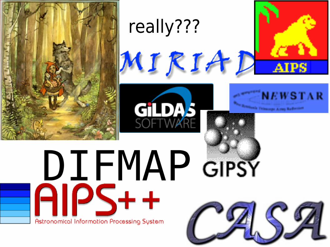
really???

DIFMAP

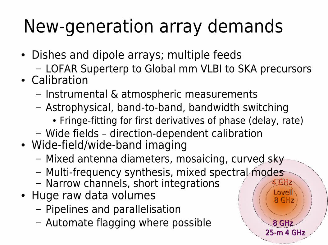
LovellLovell 8 GHz8 GHz

4 GHz4 GHz

8 GHz8 GHz25-m 4 GHz25-m 4 GHz

New-generation array demands● Dishes and dipole arrays; multiple feeds

– LOFAR Superterp to Global mm VLBI to SKA precursors● Calibration

– Instrumental & atmospheric measurements– Astrophysical, band-to-band, bandwidth switching

● Fringe-fitting for first derivatives of phase (delay, rate)– Wide fields – direction-dependent calibration

● Wide-field/wide-band imaging– Mixed antenna diameters, mosaicing, curved sky– Multi-frequency synthesis, mixed spectral modes– Narrow channels, short integrations

● Huge raw data volumes– Pipelines and parallelisation– Automate flagging where possible

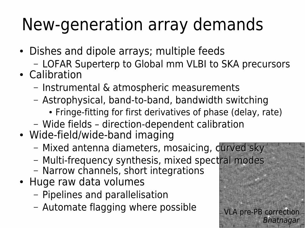
VLA pre-PB correctionBhatnagar

New-generation array demands● Dishes and dipole arrays; multiple feeds

– LOFAR Superterp to Global mm VLBI to SKA precursors● Calibration

– Instrumental & atmospheric measurements– Astrophysical, band-to-band, bandwidth switching

● Fringe-fitting for first derivatives of phase (delay, rate)– Wide fields – direction-dependent calibration

● Wide-field/wide-band imaging– Mixed antenna diameters, mosaicing, curved skycurved sky– Multi-frequency synthesis, mixed spectral modestral modes– Narrow channels, short integrations

● Huge raw data volumes– Pipelines and parallelisation– Automate flagging where possible

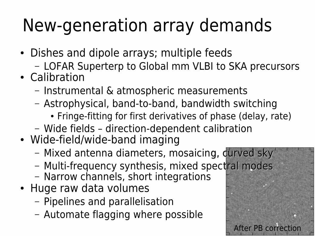
After PB correction

New-generation array demands● Dishes and dipole arrays; multiple feeds

– LOFAR Superterp to Global mm VLBI to SKA precursors● Calibration

– Instrumental & atmospheric measurements– Astrophysical, band-to-band, bandwidth switching

● Fringe-fitting for first derivatives of phase (delay, rate)– Wide fields – direction-dependent calibration

● Wide-field/wide-band imaging– Mixed antenna diameters, mosaicing, curved skyg, curved sky– Multi-frequency synthesis, mixed spectral modestral modes– Narrow channels, short integrations

● Huge raw data volumes– Pipelines and parallelisation– Automate flagging where possible

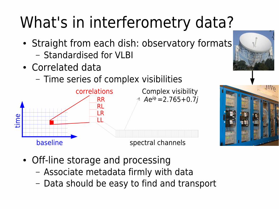
What's in interferometry data?● Straight from each dish: observatory formats

– Standardised for VLBI● Correlated data

– Time series of complex visibilities

● Off-line storage and processing– Associate metadata firmly with data– Data should be easy to find and transport

baseline

correlations

tim

e

RRRLLRLL

spectral channels

Complex visibility Aei=2.765+0.7j

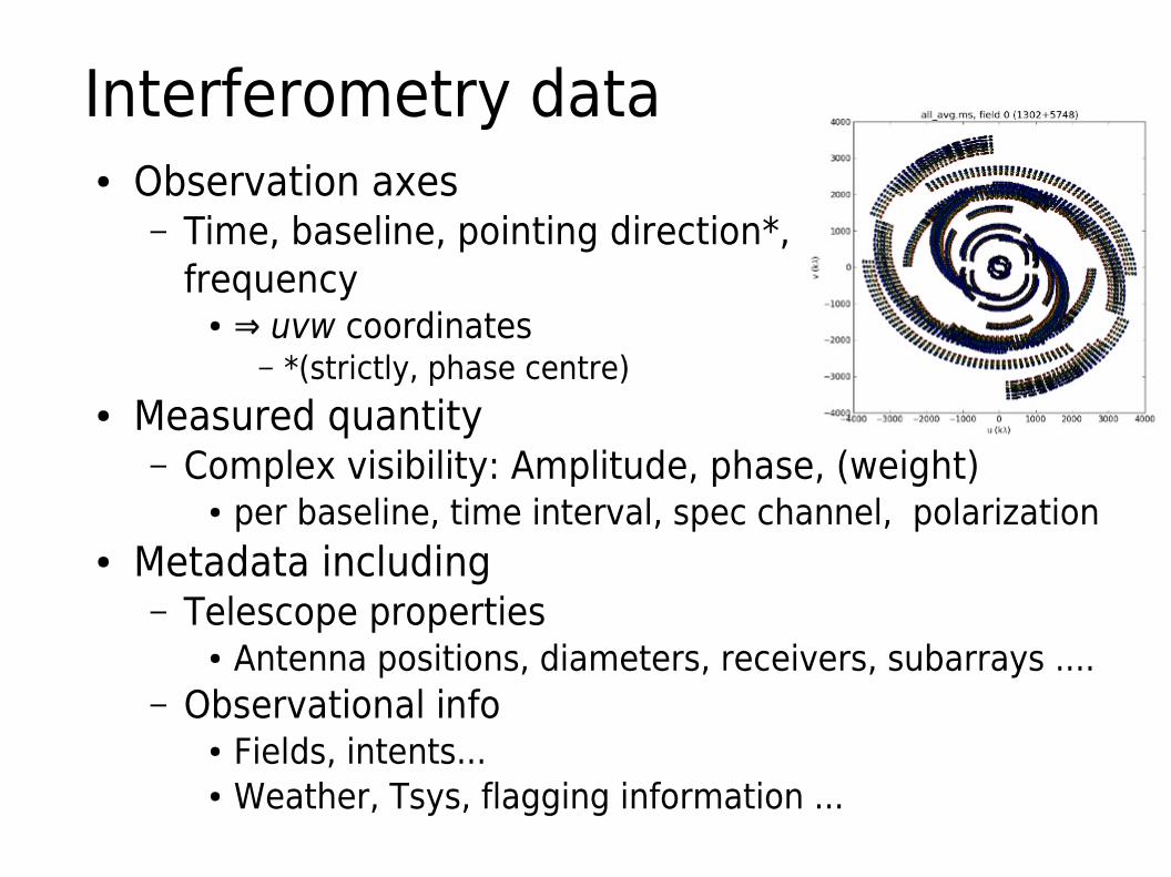
Interferometry data● Observation axes

– Time, baseline, pointing direction*, frequency

● ⇒ uvw coordinates– *(strictly, phase centre)

● Measured quantity – Complex visibility: Amplitude, phase, (weight)

● per baseline, time interval, spec channel, polarization● Metadata including

– Telescope properties● Antenna positions, diameters, receivers, subarrays ....

– Observational info● Fields, intents...● Weather, Tsys, flagging information ...

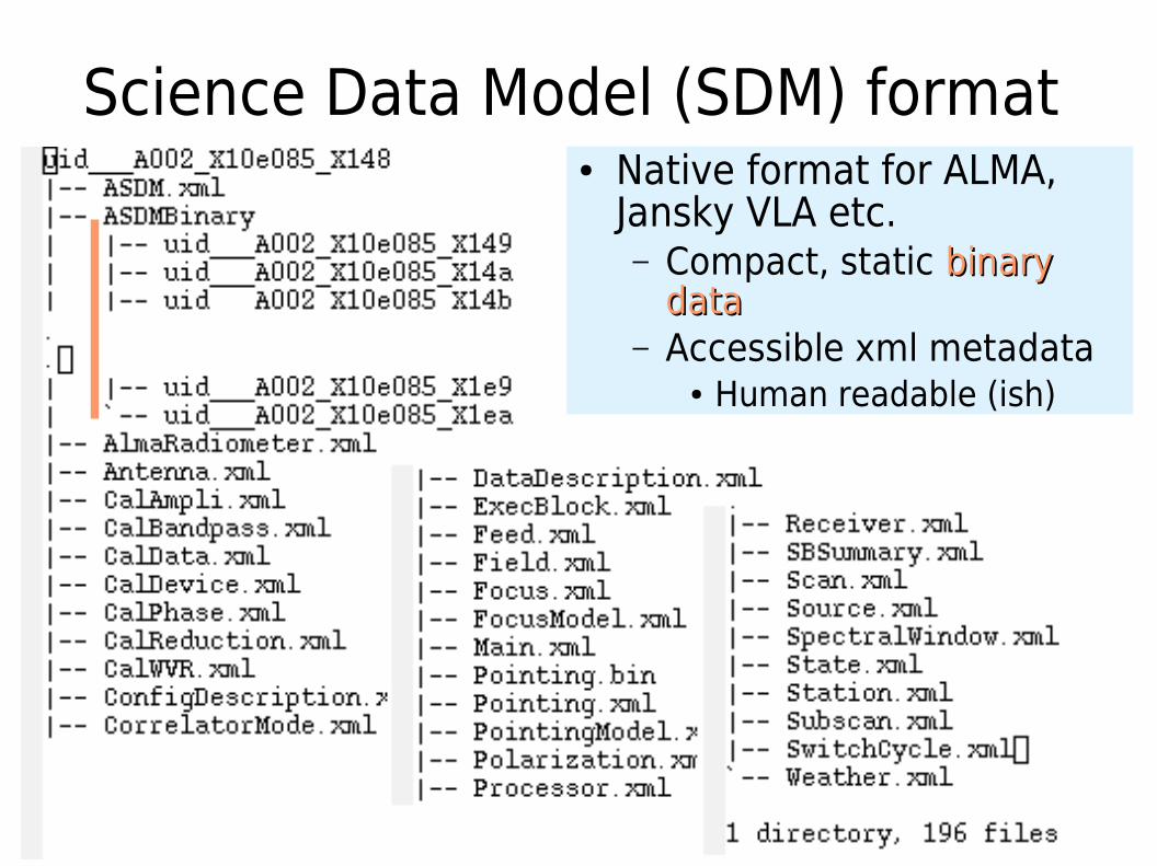
Science Data Model (SDM) format● Native format for ALMA,

Jansky VLA etc.– Compact, static binary binary

datadata– Accessible xml metadata

● Human readable (ish)

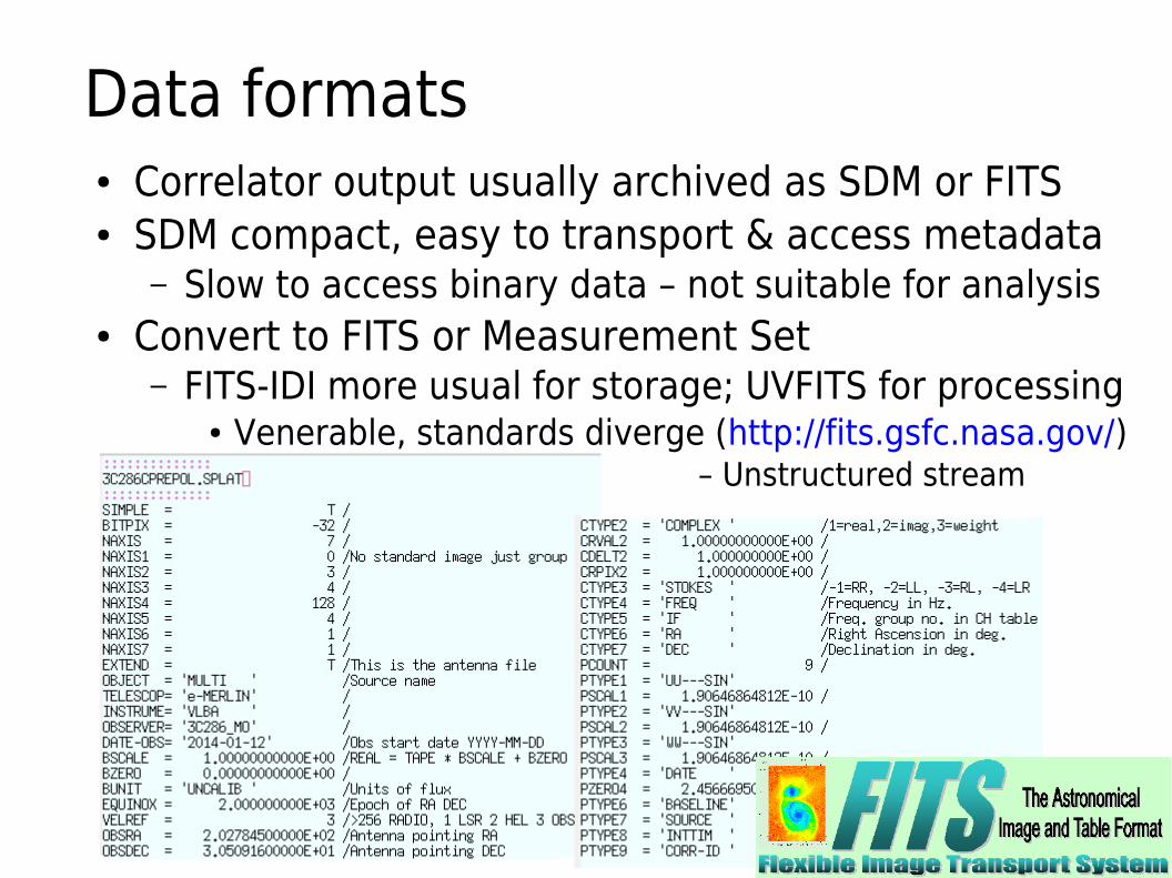
Data formats● Correlator output usually archived as SDM or FITS● SDM compact, easy to transport & access metadata

– Slow to access binary data – not suitable for analysis● Convert to FITS or Measurement Set

– FITS-IDI more usual for storage; UVFITS for processing● Venerable, standards diverge (http://fits.gsfc.nasa.gov/)

– Unstructured stream

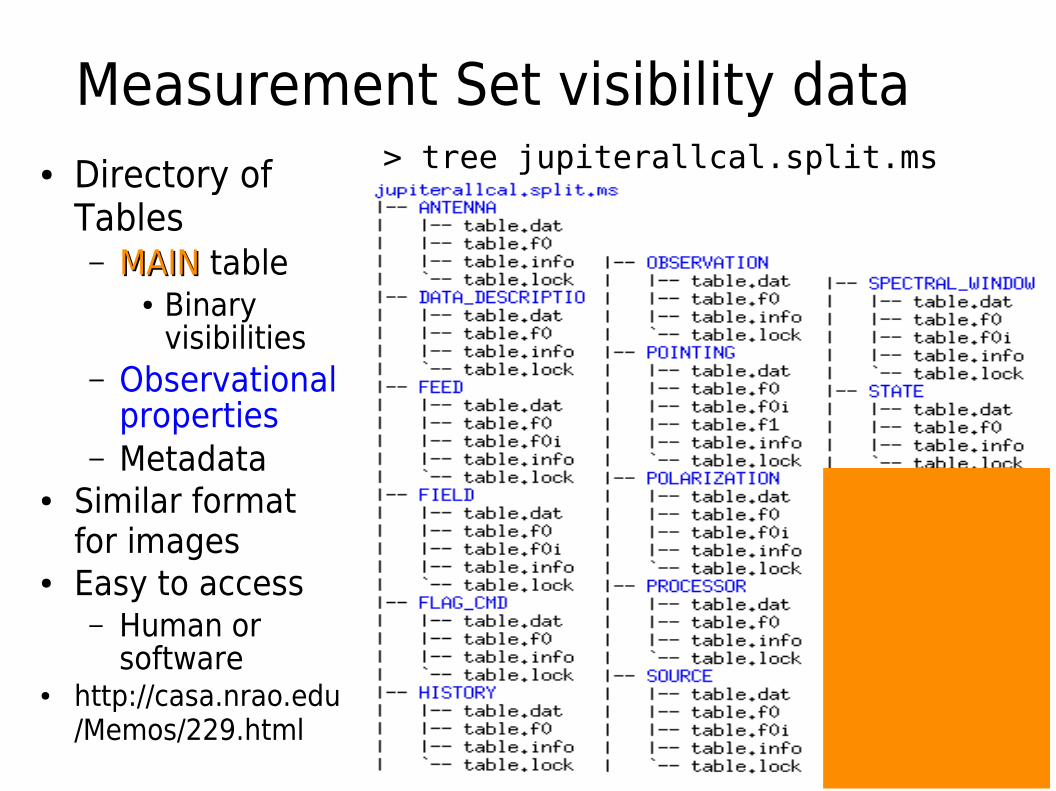
Measurement Set visibility data● Directory of

Tables– MAIN MAIN table

● Binary visibilities

– Observational properties

– Metadata● Similar format

for images● Easy to access

– Human or software

● http://casa.nrao.edu/Memos/229.html

> tree jupiterallcal.split.ms

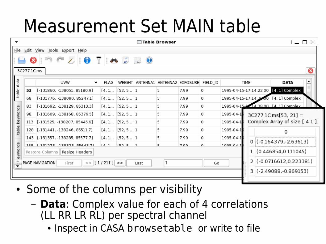
Measurement Set MAIN table

● Some of the columns per visibility– Data: Complex value for each of 4 correlations

(LL RR LR RL) per spectral channel● Inspect in CASA browsetable or write to file

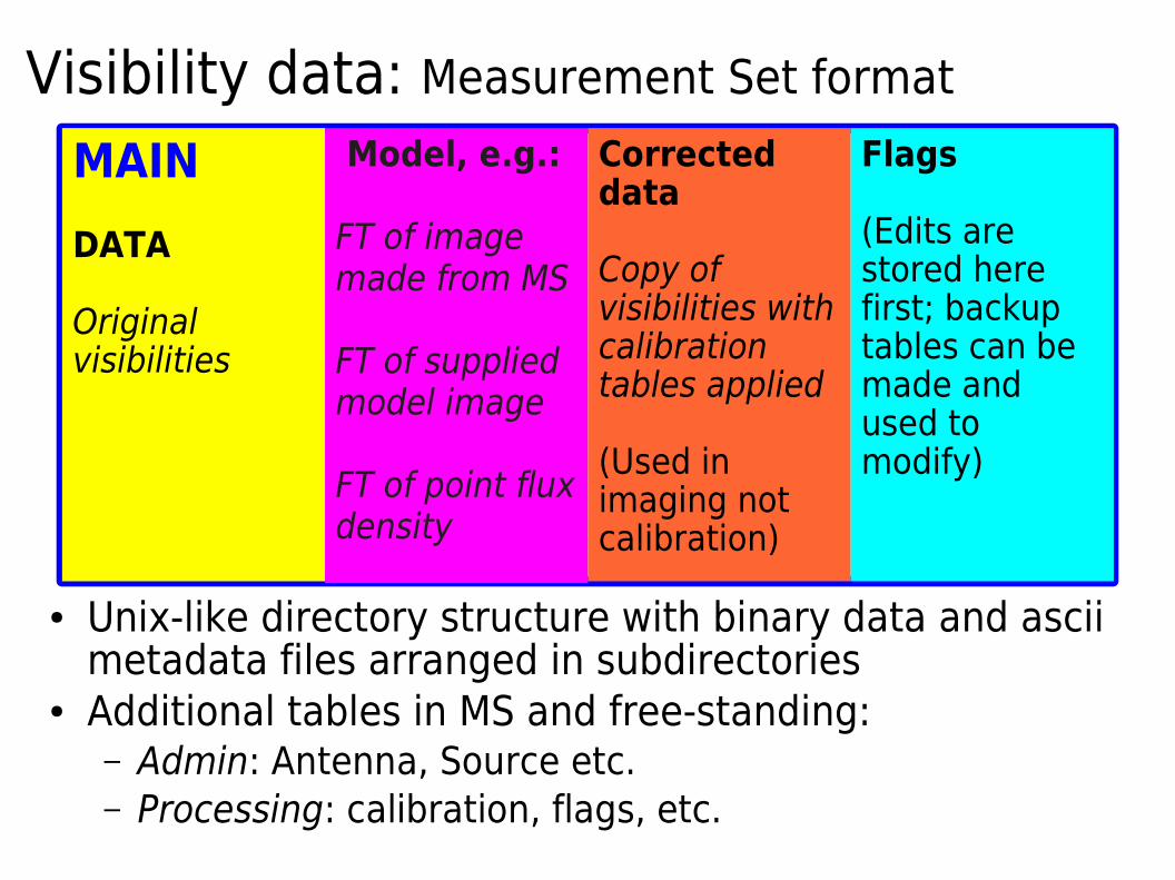
Visibility data: Measurement Set format

● Unix-like directory structure with binary data and ascii metadata files arranged in subdirectories

● Additional tables in MS and free-standing:– Admin: Antenna, Source etc.– Processing: calibration, flags, etc.

MAIN

DATA

Original visibilities

Model, e.g.:

FT of image made from MS

FT of supplied model image

FT of point flux density

Corrected data Copy of visibilities with calibration tables applied

(Used in imaging not calibration)

Flags

(Edits are stored here first; backup tables can be made and used to modify)

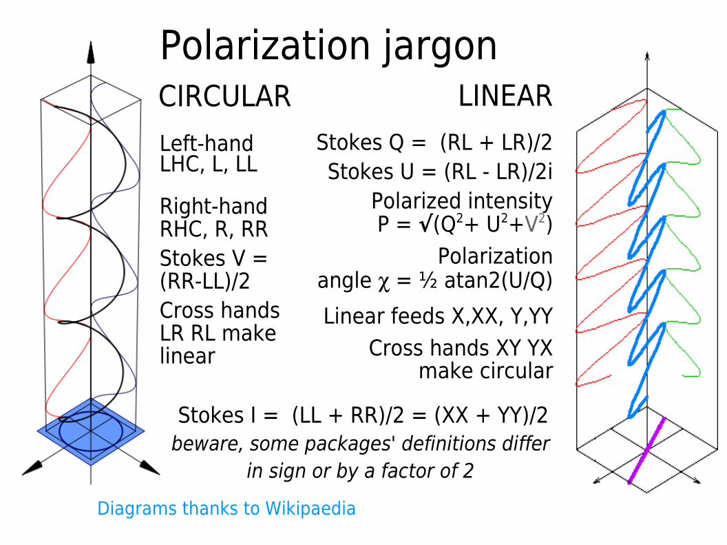
Polarization jargonLINEAR

Stokes Q = (RL + LR)/2 Stokes U = (RL - LR)/2i Polarized intensity

P = √(Q2+ U2+V2) Polarization

angle = ½ atan2(U/Q)

Linear feeds X,XX, Y,YYCross hands XY YX

make circular

Diagrams thanks to Wikipaedia

Left-hand LHC, L, LL

Right-hand RHC, R, RR Stokes V = (RR-LL)/2Cross hands LR RL make linear

CIRCULAR

Stokes I = (LL + RR)/2 = (XX + YY)/2beware, some packages' definitions differ

in sign or by a factor of 2

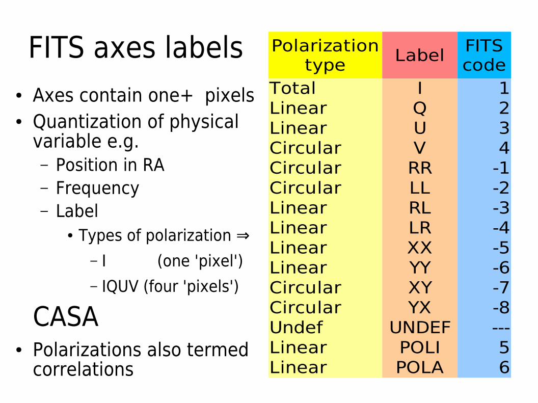
FITS axes labels Label

Total I 1Linear Q 2Linear U 3Circular V 4Circular RR -1Circular LL -2Linear RL -3Linear LR -4Linear XX -5Linear YY -6Circular XY -7Circular YX -8Undef UNDEF ---Linear POLI 5Linear POLA 6

Polarization type

FITS code

● Axes contain one+ pixels● Quantization of physical

variable e.g.– Position in RA– Frequency– Label

● Types of polarization ⇒– I (one 'pixel')– IQUV (four 'pixels')

CASA● Polarizations also termed

correlations

Data Reduction Package requirements● Import data and metadata● Derive and apply calibration

– Tables provided with data, may need converting● e.g. Tsys

– User-supplied parameters● e.g. antenna position corrections

– Calibration derived from observed sources● Bandpass, phase-reference, self-calibration...

● Display and report data properties– Flagging

● Fourier transform and produce images and spectra– Clean algorithm, maybe Maximum Entropy– Mosaicing, weighting/tapering ...

● Image analysis

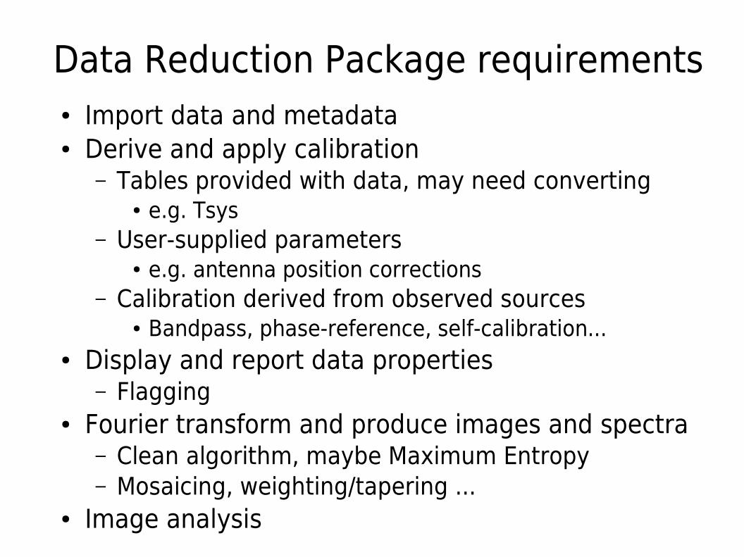
Data Reduction Package requirements● Import data and metadata● Derive and apply calibration

– Tables provided with data, may need converting● e.g. Tsys

– User-supplied parameters● e.g. antenna position corrections

– Calibration derived from observed sources● Bandpass, phase-reference, self-calibration...

● Display and report data properties– Flagging

● Fourier transform and produce images and spectra– Clean algorithm, maybe Maximum Entropy– Mosaicing, weighting/tapering ...

● Image analysis

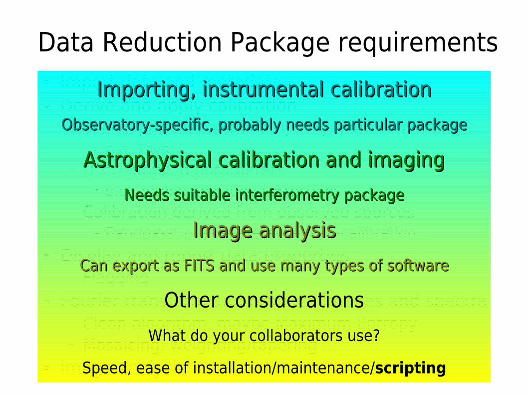
Importing, instrumental calibrationImporting, instrumental calibration

Observatory-specific, probably needs particular packageObservatory-specific, probably needs particular package

Astrophysical calibration and imagingAstrophysical calibration and imaging

Needs suitable interferometry packageNeeds suitable interferometry package

Image analysisImage analysis

Can export as FITS and use many types of softwareCan export as FITS and use many types of software

Other considerations

What do your collaborators use?

Speed, ease of installation/maintenance/scripting

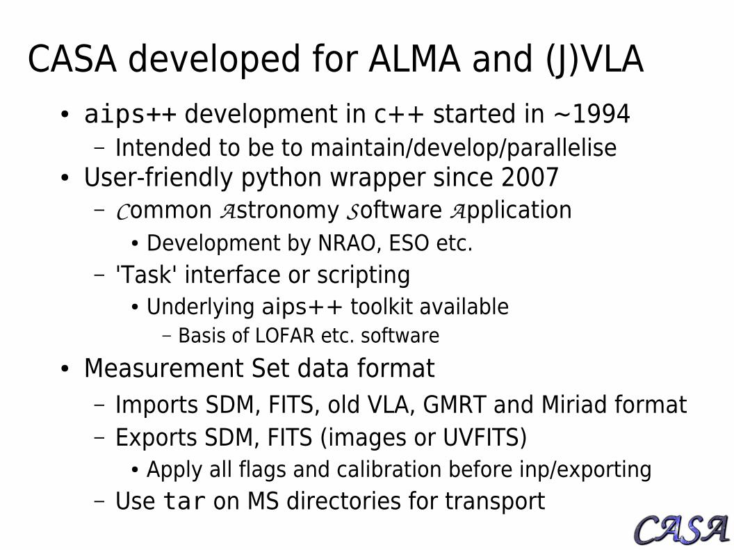
CASA developed for ALMA and (J)VLA● aips++ development in c++ started in ~1994

– Intended to be to maintain/develop/parallelise● User-friendly python wrapper since 2007

– Common Astronomy Software Application ● Development by NRAO, ESO etc.

– 'Task' interface or scripting ● Underlying aips++ toolkit available

– Basis of LOFAR etc. software● Measurement Set data format

– Imports SDM, FITS, old VLA, GMRT and Miriad format– Exports SDM, FITS (images or UVFITS)

● Apply all flags and calibration before inp/exporting– Use tar on MS directories for transport

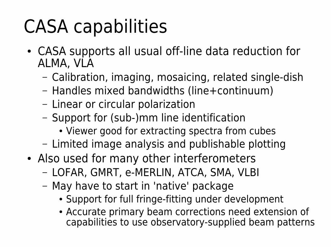
CASA capabilities● CASA supports all usual off-line data reduction for

ALMA, VLA– Calibration, imaging, mosaicing, related single-dish– Handles mixed bandwidths (line+continuum)– Linear or circular polarization– Support for (sub-)mm line identification

● Viewer good for extracting spectra from cubes– Limited image analysis and publishable plotting

● Also used for many other interferometers– LOFAR, GMRT, e-MERLIN, ATCA, SMA, VLBI– May have to start in 'native' package

● Support for full fringe-fitting under development● Accurate primary beam corrections need extension of

capabilities to use observatory-supplied beam patterns

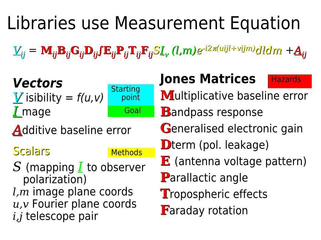
VectorsVV isibility = f(u,v)I I mage

AAdditive baseline error

ScalarsScalars

S (mapping I to observer polarization)

l,m image plane coordsu,v Fourier plane coordsi,j telescope pair

Libraries use Measurement Equation

Goal

Starting point

Hazards

Methods

VVijij = MMijijBBijijGGijijDDijij∫∫EEijijPPijijTTijijFFijijSSII (l,m)(l,m)ee-i2-i2(uijl+vijm)(uijl+vijm)dldm dldm +AAijij

Jones MatricesMMultiplicative baseline error

BBandpass response

GGeneralised electronic gain

DDterm (pol. leakage)

EE (antenna voltage pattern)

PParallactic angle

TTropospheric effects

FFaraday rotation

Using the Measurement Equation● Hamaker, Bregman & Sault 1996

– Decompose into relevant calibration components e.g.

● Vijobs = BBijijGGijijDDijijPPijijTTijijFFijijVVijij

idealideal

– Chose one (or a few) at a time● Usually solve fastest-varying first

– (so averaging over slower-varying)

– Compare data with model or idealisation● Linearise and solve by 2 (or other) minimization

– (AIPS etc. use similar algorithms for gain calibration) ● Visibility data are stored in Measurement Sets

– Accessible directories of tables

Starting CASA● See web links for downloads (or http://casa.nrao.edu)

– Don't forget the Cookbook!● Start like <path>/casa-release-4.4.0-el15/casapy

– You can set up an alias or whatever is convenient● Don't reduce data inside the CASA installation!

– This starts the iPython environment● Interactive input to tasks in the xterm● Logger (see toolbar for display, export options)

– Access to shell ● Direct simple commands e.g. ls● Prefix any shell command with ! e.g. !more *py

● Python– Case sensitive– Zero indexed (e.g. 27 antennas numbered 0~26)

● Run any scripts or functions you want

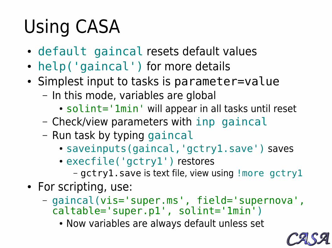
Using CASA● default gaincal resets default values● help('gaincal') for more details● Simplest input to tasks is parameter=value

– In this mode, variables are global ● solint='1min' will appear in all tasks until reset

– Check/view parameters with inp gaincal– Run task by typing gaincal

● saveinputs(gaincal,'gctry1.save') saves● execfile('gctry1') restores

– gctry1.save is text file, view using !more gctry1● For scripting, use:

– gaincal(vis='super.ms', field='supernova', caltable='super.p1', solint='1min')

● Now variables are always default unless set

Astronomical Image Processing System

● Originated by NRAO for VLA in 1978– Fortran, C– Limited built-in scripting/math operations– Historically most widely used package for cm-wave

● VLA, MERLIN, VLBI ... many more interferometers● Some support for single dish and any FITS images

– Very wide functionality from calibration to analysis● Specialised VLBI calibration and elderly formats● Many sophisticated image analysis tasks

– Lovely postscript plots for publication ● Python wrapper (Parseltongue) for easier scripting

AIPS jargon● Major operations are performed using Tasks

– FITLD loads data, CALIB performs calibration etc.● Input parameters to Tasks are set by Verbs

– >Task 'CALIB'; CALSOUR 'MKN273'; SOLINT 1– Words/names in 'inverted commas'; numbers bare– Not case sensitive, in general– Inside AIPS, 12-character limit on file/source names

● To set all defaults: >RESTORE 0– Beware: will give values typical for VLA data

● You will have to set parameters suitable for your data● To exit and kill all AIPS windows: >KLEENEX

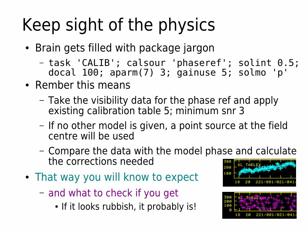
Keep sight of the physics● Brain gets filled with package jargon

– task 'CALIB'; calsour 'phaseref'; solint 0.5; docal 100; aparm(7) 3; gainuse 5; solmo 'p'

● Rember this means– Take the visibility data for the phase ref and apply

existing calibration table 5; minimum snr 3– If no other model is given, a point source at the field

centre will be used– Compare the data with the model phase and calculate

the corrections needed● That way you will know to expect

– and what to check if you get ● If it looks rubbish, it probably is!

Keep a full processing history

● Use scripts, or● Note parameter

values

−Examples for further processing

−Troubleshooting postmortem

Autopsy Tools

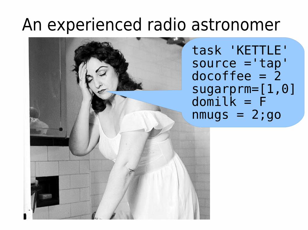
An experienced radio astronomertask 'KETTLE' source ='tap' docoffee = 2 sugarprm=[1,0] domilk = F nmugs = 2;go