radar sensing of ocean wave heights a thesis submitted to ... · radar sensing of ocean wave...
TRANSCRIPT
RADAR SENSING OF OCEAN WAVE HEIGHTS
A THESIS SUBMITTED TO THE GRADUATE DIVISION OF THEUNIVERSITY OF HAWAI‘I IN PARTIAL FULFILLMENT
OF THE REQUIREMENTS FOR THE DEGREE OF
MASTER OF SCIENCE
IN
OCEANOGRAPHY
DECEMBER 2010
ByTyson Hilmer
Thesis Committee:
Mark Merrifield, ChairpersonPierre FlamentDouglas Luther

This work is dedicated to
my beautiful wife Susanne
for her unequivocal patience
ii

Figure 0.1
iii

Acknowledgements
I would like to thank my advisor, Pierre Flament, and the other members of my M.S.
committee, Mark Merrifield, and Doug Luther for all their feedback. I am thankful to Jerome
Aucan for his assistance with the CDIP buoy data, and to Jim Potemra for assistance with archived
IPRC data. Special thanks to my friends and family for encouragement and support throughout this
project.
Radar data were furnished by the Radio Oceanography Laboratory, Department of Oceanog-
raphy, University of Hawaii at Manoa. Buoy data were furnished by the Coastal Data Informa-
tion Program (CDIP), Integrative Oceanography Division, operated by the Scripps Institution of
Oceanography, under the sponsorship of the U.S. Army Corps of Engineers and the California
Department of Boating and Waterways. Multi-Spectral Model (MSM) wind model output were
furnished by Yi-Leng Chen, Department of Meteorology, University of Hawaii.
iv

ABSTRACT
This thesis focuses on explaining and improving the estimation of ocean wave heights
from high-frequency oceanographic radar. Three months of data from a WERA HF radar is com-
pared to a Datawell MarkIII directional waverider buoy, under a wide range of sea states. Large
spatial and temporal variation in the radar-derived waveheight, significantly greater than previously
reported, are explained in terms of various error sources. Averaging and filtering methods for im-
proving the significant waveheight are evaluated, and the dominant error source is shown to be
external radio frequency interference. Eigen-analysis and model-based methods are evaluated for
the removal of interference. A comprehensive summary of the second order radar-ocean scattering
equations is given, with evaluation of its terms.
v
Contents
Acknowledgements iv
Abstract v
List of Tables viii
List of Figures ix
1 Introduction 11.1 Applications . . . . . . . . . . . . . . . . . . . . . . . . . . . . . . . . . . . . . . 21.2 Operational Description of Oceanographic Radars . . . . . . . . . . . . . . . . . . 21.3 Development History . . . . . . . . . . . . . . . . . . . . . . . . . . . . . . . . . 71.4 Electromagnetic Scattering Theory . . . . . . . . . . . . . . . . . . . . . . . . . . 71.5 Previous Research . . . . . . . . . . . . . . . . . . . . . . . . . . . . . . . . . . . 19
1.5.1 Currents . . . . . . . . . . . . . . . . . . . . . . . . . . . . . . . . . . . . 191.5.2 Winds . . . . . . . . . . . . . . . . . . . . . . . . . . . . . . . . . . . . . 201.5.3 Waves . . . . . . . . . . . . . . . . . . . . . . . . . . . . . . . . . . . . . 25
2 Methods 322.1 WERA radar and directional wave buoy . . . . . . . . . . . . . . . . . . . . . . . 322.2 Processing . . . . . . . . . . . . . . . . . . . . . . . . . . . . . . . . . . . . . . . 37
3 Results 433.1 Winds . . . . . . . . . . . . . . . . . . . . . . . . . . . . . . . . . . . . . . . . . 433.2 Significant Waveheight . . . . . . . . . . . . . . . . . . . . . . . . . . . . . . . . 473.3 Noise Error . . . . . . . . . . . . . . . . . . . . . . . . . . . . . . . . . . . . . . 56
3.3.1 Introduction . . . . . . . . . . . . . . . . . . . . . . . . . . . . . . . . . . 563.3.2 Observations . . . . . . . . . . . . . . . . . . . . . . . . . . . . . . . . . 573.3.3 Noise Estimation . . . . . . . . . . . . . . . . . . . . . . . . . . . . . . . 643.3.4 Noise Removal . . . . . . . . . . . . . . . . . . . . . . . . . . . . . . . . 73
3.4 Significant Waveheight Regression Analysis . . . . . . . . . . . . . . . . . . . . . 803.5 Electromagnetic Scattering: Second Order Integral . . . . . . . . . . . . . . . . . 833.6 Spectral Averaging . . . . . . . . . . . . . . . . . . . . . . . . . . . . . . . . . . 88
vi

4 Discussion 934.1 Wind Estimates . . . . . . . . . . . . . . . . . . . . . . . . . . . . . . . . . . . . 934.2 Significant Waveheight Estimates . . . . . . . . . . . . . . . . . . . . . . . . . . . 94
5 Conclusion 99
Appendices 100
A Electromagnetic Scattering Derivations 101A.1 Ground Wave Propagation . . . . . . . . . . . . . . . . . . . . . . . . . . . . . . 101A.2 Ground Wave Scatter . . . . . . . . . . . . . . . . . . . . . . . . . . . . . . . . . 103A.3 Far Field Scatter . . . . . . . . . . . . . . . . . . . . . . . . . . . . . . . . . . . . 106A.4 Average Scattered Signal Spectrum . . . . . . . . . . . . . . . . . . . . . . . . . . 107A.5 First Order Spectrum . . . . . . . . . . . . . . . . . . . . . . . . . . . . . . . . . 109A.6 Second Order Spectrum . . . . . . . . . . . . . . . . . . . . . . . . . . . . . . . . 110
B WERA Significant Waveheight Algorithm 114
C Beamforming 117
D Vector Correlation 120
vii

List of Tables
1.1 Comparison studies of radar to buoys . . . . . . . . . . . . . . . . . . . . . . . . . 31
3.1 Hs error analysis . . . . . . . . . . . . . . . . . . . . . . . . . . . . . . . . . . . 52
viii

List of Figures
1.1 Radar Doppler Spectrum . . . . . . . . . . . . . . . . . . . . . . . . . . . . . . . 31.2 Vector current estimate from two radial components . . . . . . . . . . . . . . . . . 41.3 Geographic Dilution of Precision . . . . . . . . . . . . . . . . . . . . . . . . . . . 51.4 Bragg scattering diagram . . . . . . . . . . . . . . . . . . . . . . . . . . . . . . . 81.5 Electromagnetic scattering diagram . . . . . . . . . . . . . . . . . . . . . . . . . 101.6 Hydrodynamic scattering diagram . . . . . . . . . . . . . . . . . . . . . . . . . . 111.7 Hydrodynamic scattering diagram: closeup . . . . . . . . . . . . . . . . . . . . . 121.8 EM scattering geometry . . . . . . . . . . . . . . . . . . . . . . . . . . . . . . . . 131.9 Bistatic radar geometry . . . . . . . . . . . . . . . . . . . . . . . . . . . . . . . . 151.10 Bragg ratio diagram . . . . . . . . . . . . . . . . . . . . . . . . . . . . . . . . . . 221.11 Bragg ratio vs Angle for a variety of different spreading models . . . . . . . . . . 231.12 Bragg ratio vs. in-situ wind directions . . . . . . . . . . . . . . . . . . . . . . . . 251.13 Radar to Buoy wind estimate comparison . . . . . . . . . . . . . . . . . . . . . . 261.14 Linearized form of Hs . . . . . . . . . . . . . . . . . . . . . . . . . . . . . . . . . 28
2.1 Example CDIP buoy energy spectrum . . . . . . . . . . . . . . . . . . . . . . . . 332.2 Example CDIP buoy directional spectrum . . . . . . . . . . . . . . . . . . . . . . 342.3 Radar sampling geometry . . . . . . . . . . . . . . . . . . . . . . . . . . . . . . . 352.4 Temporal coverage and study period . . . . . . . . . . . . . . . . . . . . . . . . . 362.5 Buoy significant wave height Hm0 timeseries . . . . . . . . . . . . . . . . . . . . . 362.6 Example Doppler spectra . . . . . . . . . . . . . . . . . . . . . . . . . . . . . . . 382.7 Hs errors due to difference search algorithm . . . . . . . . . . . . . . . . . . . . . 392.8 Bragg centroid frequency . . . . . . . . . . . . . . . . . . . . . . . . . . . . . . . 402.9 Bragg frequency; comparison of centroid vs. peak method . . . . . . . . . . . . . 412.10 Distribution of difference in Bragg frequency methods . . . . . . . . . . . . . . . 42
3.1 Multi-Spectral Model grid . . . . . . . . . . . . . . . . . . . . . . . . . . . . . . 443.2 QuickSCAT winds for the Hawaiian Islands . . . . . . . . . . . . . . . . . . . . . 443.3 Example radar-derived wind field . . . . . . . . . . . . . . . . . . . . . . . . . . . 453.4 Radar wind field compared to MSM output . . . . . . . . . . . . . . . . . . . . . 453.5 Radar wind field compared to QuickSCAT . . . . . . . . . . . . . . . . . . . . . . 463.6 Hs timeseries for CDIP buoy and radar . . . . . . . . . . . . . . . . . . . . . . . . 473.7 Spatial and temporal variation in radar Hs field . . . . . . . . . . . . . . . . . . . 483.8 Hs linear regression between CDIP buoy and radar . . . . . . . . . . . . . . . . . 483.9 Hs linear regression between CDIP buoy and radar timeseries . . . . . . . . . . . . 49
ix
3.10 Hs power law regression . . . . . . . . . . . . . . . . . . . . . . . . . . . . . . . 503.11 Hs power law regression; spatial average . . . . . . . . . . . . . . . . . . . . . . . 513.12 Radar and buoy Hs distributions . . . . . . . . . . . . . . . . . . . . . . . . . . . 523.13 Hsdirectional dependence algorithm comparison . . . . . . . . . . . . . . . . . . . 533.14 Theoretical and observed Hs spatial correlation . . . . . . . . . . . . . . . . . . . 543.15 Hs mean; 1 day . . . . . . . . . . . . . . . . . . . . . . . . . . . . . . . . . . . . 553.16 Hs 21 day median . . . . . . . . . . . . . . . . . . . . . . . . . . . . . . . . . . . 553.17 Example low and high noise antenna spectra . . . . . . . . . . . . . . . . . . . . . 583.18 Radio interference in second order region . . . . . . . . . . . . . . . . . . . . . . 593.19 A well-resolved Doppler spectrum . . . . . . . . . . . . . . . . . . . . . . . . . . 603.20 A poorly-resolved Doppler spectrum . . . . . . . . . . . . . . . . . . . . . . . . . 613.21 Example low and high noise fields . . . . . . . . . . . . . . . . . . . . . . . . . . 623.22 Noise CDF estimates . . . . . . . . . . . . . . . . . . . . . . . . . . . . . . . . . 653.23 Spectral histogram of noise levels . . . . . . . . . . . . . . . . . . . . . . . . . . 663.24 Noise distribution for Kaena and Koolina . . . . . . . . . . . . . . . . . . . . . . 673.25 Cumulative Signal-to-Noise Ratio . . . . . . . . . . . . . . . . . . . . . . . . . . 683.26 201 noise source, world map . . . . . . . . . . . . . . . . . . . . . . . . . . . . . 693.27 Sampling field of the JORN radar . . . . . . . . . . . . . . . . . . . . . . . . . . 693.28 Noise level as a function of angle and time . . . . . . . . . . . . . . . . . . . . . . 703.29 Noise level as a function of range and time . . . . . . . . . . . . . . . . . . . . . . 703.30 Functional noise model . . . . . . . . . . . . . . . . . . . . . . . . . . . . . . . . 713.31 Noise model: NI(θ, t) term . . . . . . . . . . . . . . . . . . . . . . . . . . . . . . 723.32 MUSIC algorithm results . . . . . . . . . . . . . . . . . . . . . . . . . . . . . . . 753.33 Noise as a function of beam-steered direction . . . . . . . . . . . . . . . . . . . . 763.34 Range eigenfunctions . . . . . . . . . . . . . . . . . . . . . . . . . . . . . . . . . 763.35 Range eigenfunctions; noise only . . . . . . . . . . . . . . . . . . . . . . . . . . . 773.36 RFI phase difference . . . . . . . . . . . . . . . . . . . . . . . . . . . . . . . . . 783.37 RFI removal results . . . . . . . . . . . . . . . . . . . . . . . . . . . . . . . . . . 783.38 RFI removal; effect of incorrect phase . . . . . . . . . . . . . . . . . . . . . . . . 793.39 Hs linear regression coefficients . . . . . . . . . . . . . . . . . . . . . . . . . . . 813.40 Hs linear regression; coefficient of determination . . . . . . . . . . . . . . . . . . 823.41 Hs linear regression; RMS error . . . . . . . . . . . . . . . . . . . . . . . . . . . 823.42 Second order Doppler-Wavevector relation . . . . . . . . . . . . . . . . . . . . . . 843.43 Hydrodynamic and Electromagnetic Coupling Coefficients . . . . . . . . . . . . . 853.44 S2 integral product . . . . . . . . . . . . . . . . . . . . . . . . . . . . . . . . . . 863.45 Doppler frequency-averaged Coupling Coefficient . . . . . . . . . . . . . . . . . . 873.46 Example of spectral averaging . . . . . . . . . . . . . . . . . . . . . . . . . . . . 883.47 Spectrogram normalized by S1 . . . . . . . . . . . . . . . . . . . . . . . . . . . . 893.48 Close-up of normalized spectrogram . . . . . . . . . . . . . . . . . . . . . . . . . 903.49 Mean spectrum with outliers removed . . . . . . . . . . . . . . . . . . . . . . . . 913.50 Comparison of Hs timeseries from spectral averaging . . . . . . . . . . . . . . . . 913.51 Spectral time-evolution . . . . . . . . . . . . . . . . . . . . . . . . . . . . . . . . 92
4.1 Merging of first and second order peaks . . . . . . . . . . . . . . . . . . . . . . . 95
x

A.1 Effect of surface roughness on impedance . . . . . . . . . . . . . . . . . . . . . . 102A.2 EM transmission loss over the ocean . . . . . . . . . . . . . . . . . . . . . . . . . 103
B.1 Directional spreading functions . . . . . . . . . . . . . . . . . . . . . . . . . . . . 115
C.1 Beamforming array pattern . . . . . . . . . . . . . . . . . . . . . . . . . . . . . . 118
xi
Chapter 1
Introduction
The data products from oceanographic radars can be separated into two fundamental cat-
egories delineated by the interaction mechanism of remote measurement. Foremost is first order
scattering, due to coherent reflection of the electromagnetic wave off linear ocean waves of a fixed
wavelength. The other mechanism is second order scattering, caused by similar coherent reflec-
tions off the continuum of nonlinear ocean waves. These two scattering mechanisms differ in how
the information content is encoded in the radar signal, and by the physical process measured. The
frequency shift of first order scatter allows oceanographic radars to generate large two dimensional
maps of ocean surface currents. The scattering mechanism is relatively simple, and frequency differ-
ences are a robust radar measurement. The spectral amplitudes of second order scatter contains in-
formation about the full 2-dimensional sea surface, and consequently the directional wave spectrum.
The scattering mechanism is relatively complex, and the measurement is not uniquely determined.
Furthermore, the information carried in spectral amplitudes is sensitive to instrument performance
and noise sources.
The motivation for this work is to further understanding and accuracy of the second order
radar measurement. HF radars are unique in their ability to provide dense three-dimensional obser-
vations which are outside the scope of other instruments. Prior success in ocean wave measurement
via HF radar has been demonstrated, but there is a demand for further observation and validation.
The theoretical and empirical relationship between the radar Doppler spectrum and ocean surface is
1
an ongoing field of study. Much of this thesis focuses on how the Doppler spectrum is processed to
yield oceanographic parameters, primarily significant waveheight.
1.1 Applications
Oceanographic radar is capable of providing wide-area measurements that are difficult or
impossible to make any other way. Their development and application as an oceanographic research
tool began in 1955, and their performance is now widely established. Using electromagnetic and
hydrodynamic theory, it is possible to infer information about the ocean surface; primarily its shape
and velocity, from the radar Doppler spectrum. Radar provides continuous, synoptic measurement
of physical oceanographic properties; two-dimensional spatial maps of surface-current vectors, the
surface wave directional spectrum, significant waveheight, and surface wind direction. The benefit
of radar over conventional in-situ instruments is the spatial measurement field; typically O(10,000)
measurement points over a 2-dimensional area, with range depending on the transmit frequency.
Comparable in-situ instruments, such as buoys, pressure sensors, ADCPs, and ECMs, provide rel-
atively smaller spatial coverage or a point measurement. Conversely, satellite remote sensing; e.g.
radar altimeters, synthetic aperature radars, scatterometers, and microwave radiometers, provide
relatively coarser spatial coverage over a larger region. Complete spatial fields are available every
10-30 minutes, dependent on the coherent integration time of the spectra. The majority of radar
installations are shore based, although several ship-board experiments have been conducted [Gurgel
and Essen, 2000].
The large observational area and near real-time availability of oceanographic radar of-
fers a variety of real-world applications. They are capable of monitoring sea state and weather
conditions, whilst simultaneously tracking ships and even iceburgs. Current maps aid in oil spill
containment and search-and-rescue operations. Ship and object detection is used for vessel traffic
control and Exclusive Economic Zone enforcement. Wind estimates are useful for detecting frontal
boundaries [Fernandez et al., 1997] and other sudden changes in direction, e.g. small-scale storms
and waterspouts. While sea state monitoring is used for engineering projects, and safety conditions
for beaches and the recreational nearshore.
1.2 Operational Description of Oceanographic Radars
Oceanographic radars typically operate in the High-Frequency (HF) radio band (3-30
MHz), and at very low power (30 W). The radar transmits a nearly monochromatic electromag-
2
−2 −1 0 1 240
60
80
100
120
140
160
Doppler Frequency (Hz)
Po
wer
(dB
)
σ1
σ2
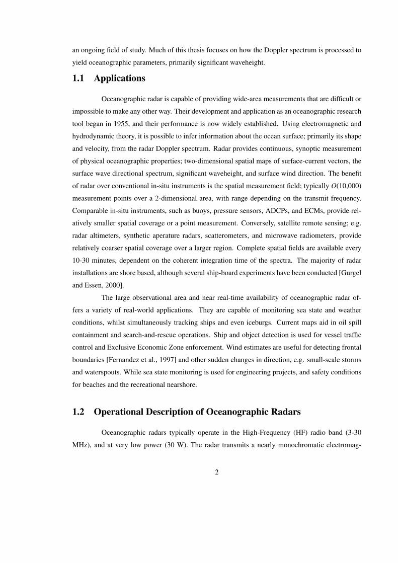
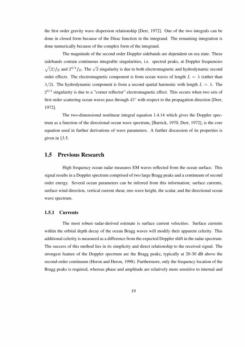
Figure 1.1: An example radar Doppler spectrum. First order Bragg peaks are located at ∼ 0.5
Hz [σ1]. This Bragg frequency for this instrument is 0.409 Hz [dashed vertical lines]; the positive
frequency difference between observed and expected Bragg frequency indicates a radial current
moving toward the radar. The second order continuum [σ2] is adjacent to the Bragg peaks. The
noise floor for this spectrum is ∼ 60 dB [dashed horizontal line].
netic (EM) wave which propagates as a trapped ground wave along the conductive surface of the
ocean. The EM wave is scattered off the ocean surface, and some of the reflected energy is incident
on the radar’s receive antennas. The receive signal is then complex-modulated with the transmit sig-
nal to obtain the Doppler spectra (Figure 1.1). The Doppler spectrum is a measurement of variations
in the transmitted EM wave due to interactions with the physical environment. It is the fundamental
radar measurement, and must be processed via algorithms to yield oceanographic parameters.
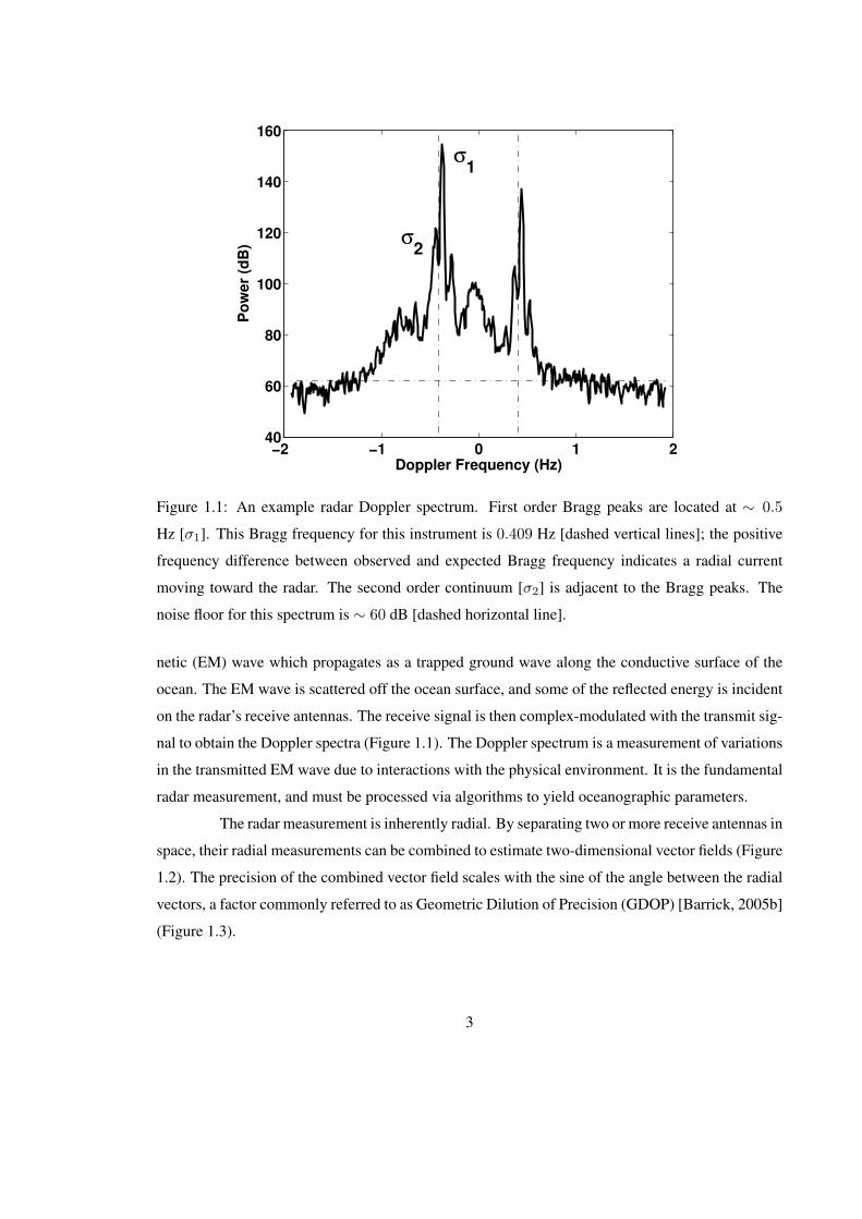
The radar measurement is inherently radial. By separating two or more receive antennas in
space, their radial measurements can be combined to estimate two-dimensional vector fields (Figure
1.2). The precision of the combined vector field scales with the sine of the angle between the radial
vectors, a factor commonly referred to as Geometric Dilution of Precision (GDOP) [Barrick, 2005b]
(Figure 1.3).
3

Figure 1.2: From Fernandez et al. [1997]. Schematic for determining the resulting vector currrent
from velocity components of two intersecting radials.
4

Figure 1.3: Geographic Dilution of Precision for the Oahu sampling grid.
5

Range resolution is obtained using coded waveforms, the most common being Frequency
Modulated Continuous Wave (FMCW). FMCW linearly sweeps over a frequency band of hundreds
of KHz, with the bandwidth determining the range resolution. Ranges are known from the constant
frequency difference between the transmitted and received signals, with maximum range determined
by operating frequency and power. Doppler spectral resolution is obtained by repeating the range
measurements and performing time-series analysis on the samples. The coherent integration time T
determines the frequency resolution ∆f = 1/T Hz. Consequently, the radial velocity resolution is
∆v = λ∆f/2 m s−1, where λ is the radar wavelength.
Angular resolution is achieved using multiple receive antennas in varying array config-
urations. Directivity is defined as a measure of the antenna array’s capability to resolve a given
direction. The minimum resolvable angle is determined by the Rayleigh criterion θR = arcsinλ/d,
where d is the antenna separation distance and λ is the EM wavelength. As the desired directivity
increases, so does the required number of antennas and length of the array. A more detailed dis-
cussion of angle determination is given in the beamforming appendix §C. HF radar is limited in its
directivity due to the relatively large EM wavelength (10-100 m for 30-3 MHz), necessitating large
arrays.
The incident angle of the receive signal can be inferred from phase differences between
multiple antennas. Currently there are two major categories of receive antenna patterns used for
oceanographic radars. One is the linear (or phased) array, typically with 8 to 16 antennas spaced one-
half wavelength apart. The large number of antennas and length of a linear array provides superior
angular resolution, at the disadvantage of considerable spatial size and other logistical requirements.
The other category of receive array is the square array. These have the logistical benefit of being
compact, but have limited angle-resolving capabilities; typically a 1:1 or 1:2 mapping between range
and direction, compared to the full 2-dimensional field of a linear array.
The algorithm used for estimating directional information also depends on the receive
array type. Square arrays use direction-finding algorithms to estimate direction, which vary in
complexity from simple geometric equations to eigen-decomposition methods. The common feature
of all direction-finding algorithms is the incidence angle must be solved for, i.e. it is a dependent
variable of the data set. Thus signal components can only arrive from a limited subset of directions;
which is a significant and necessary limiting assumption. Linear arrays use beamforming equations;
essentially directional weighting functions which apply a phase shift to each antenna, then sum. The
beamforming method allows for estimating signal from any specific direction, as the incidence angle
is an independent variable.
6
1.3 Development History
Crombie [1955] was the first to apply radar to oceanographic measurement. He identified
coherent scattering from the sea in a radar Doppler spectrum, and realized the difference between
the expected surface gravity wave and measured Doppler frequencies was due to surface current ve-
locities. Crombie [1972] examined the coherence between signals received on two closely spaced
whip antennas, and found the phase coherence varied with Doppler frequency, implying that signals
having different Doppler shifts were coming from different directions, and interpreted this as view-
ing a uniform current from different aspect angles. This result led to the development of the Coastal
Ocean Dynamic Applications Radar (CODAR) [Barrick et al., 1977, Lipa and Barrick, 1983] by the
NOAA Wave Propagation Laboratory. The 16-element phased array Ocean Surface Current Radar
(OSCR) was commercially developed by Marex Ltd., England. OSCR was used for mapping tidal
and residual currents near Britain [Prandle, 1987], and by the University of Miami for coastal obser-
vations [Shay et al., 1995, Graber et al., 1996]. A summary of nine OSCR deployments is given in
Prandle and Ryder [1985]. In 1996 the HF Wellen radar (WERA) was developed at the University
of Hamburg. WERA was designed to allow a range of radar frequencies from 5-45 MHz, range res-
olution from 2 km to 250 m, and different antenna configurations. WERA utilized new ocean wave
directional spectrum algorithms developed by the University of Sheffield, UK. Operational theory
for the WERA is described in Gurgel et al. [1999b], and system design in Gurgel et al. [1999a]. See
Teague et al. [1997] for a concise review of oceanographic radar development.
This work primarily focuses on HF groundwave radar, where the EM wave propagates
along the ocean surface. Skywave is another category of radar requiring mention. Otherwise re-
ferred to as Over-The-Horizon (OTH) radar, they function by bouncing dekametric waves off the
ionosphere. Originally developed for long-range military surveillance, skywave radar has spatial
coverage of O ·106 km2 with resolution O 10 km, whereas HF groundwave radar has O ·103 km2
coverage and O 1 km resolution. The intermediate reflections of skywave radar introduces addi-
tional processing considerations due to signal modulation and noise from the ionosphere - a feature
not shared by groundwave HF radar.
1.4 Electromagnetic Scattering Theory
For ocean surface waves of a specific wavelength relative to the incident EM wave, a
phase coherent reinforcement (constructive interference) exists in the reflected EM signal (Figure
7

Figure 1.4: Bragg scattering is coherent reflection of the EM wave [thin] by ocean waves [thick]
with wavelength λ/2 [top]. Incoherent reflections, i.e. cancellation of the EM energy, occur for
arbitrary ocean wavelengths [bottom].
1.4). This effect is known as Bragg scattering [Bragg, 1913], and the corresponding surface waves
are referred to as Bragg waves. In the literature, this effect is also labeled ”first order” or ”linear”,
as the EM-ocean wave interaction simplifies to a linear equation. The coherently reflected signal is
evident as peaks in the reflected EM spectra, offset by a Doppler shift from the transmit frequency
(Figure 1.1). This Doppler shift in the return spectra was first reported by Crombie [1955], who also
correctly surmised the celerity of the Bragg waves as the cause for the Doppler shift. From Crombie
[1955], the Doppler shift due to Bragg waves is:
∆f =c
λ=
√g
2πλ=
√g
πL(1.4.1)
where ∆f is the Doppler shift (Hz), c is the ocean wave celerity (m/s), λ is the ocean wave wave-
length (m), and L is radar electromagnetic wave wavelength (m). Crombie [1972] further observed
that the phase of the coherence varied with Doppler frequency, implying that signals having differ-
ent Doppler shifts were coming from different directions, and interpreted this as viewing a uniform
current from different aspect angles. Bragg scattering is commonly attributed to waves with one half
the EM wavelength; this is true for radars with a backscatter antenna configuration, i.e. co-located
transmit and receive antennas. Bistatic, i.e. spatially separated transmit and receive antennas, re-
quire a more general expression for Bragg scattering (§A.5).
Barrick [1970] was the first to derive a complete theory for electromagnetic waves scat-
tering from the sea surface using electromagnetic and oceanographic first principles, resulting in
8
an explicit integral representation of the Doppler spectrum in terms of the directional waveheight
spectrum of the sea. Barrick’s EM interaction equations are the fundamental basis for the use and
interpretation of oceanographic radars. Barrick [1970, 1971a,b, 1972], Derr [1972], Weber and
Barrick [1977], Barrick and Weber [1977] are seminal papers for scattering theory. For a review of
previous EM scattering research, see Saxton [1964]. The theory considers radiation and propagation
of EM waves above the sea, with attention to the effects of a variable sea surface. Barrick [1970]
is considered the theoretical confirmation of Crombie [1955], due to the theoretical prediction of
Bragg peaks in the Doppler spectrum. The equations are general in that they allow for variable
geometries for the transmit and receive antennas. Using only first order theory, the ocean wave di-
rectional spectra can be obtained by varying the antenna placement, as discussed by Barrick [1970],
numerically investigated by Nierenberg and Munk [1969], and applied by Peterson et al. [1970],
Teague [1971]; or by varying the transmit frequency [Crombie, 1970]. A full summary of Barrick’s
electromagnetic scattering derivations is given in §A.
Further theoretical work by Weber and Barrick [1977], Barrick and Weber [1977] showed
that the second order continuum of energy in the Doppler spectrum is produced by two independent
effects; an electromagnetic and a hydrodynamic. The electromagnetic component corresponds to
radar waves twice scattered from ocean waves, where the geometry of the double scattering causes
coherent reflections (Figure 1.5). The hydrodynamic component corresponds to nonlinear surface
waves which satisfy the Bragg wavelength [Barrick and Weber, 1977] via the wavevector relation
kB = k1+k2 (Figure 1.6,1.7). Both of these components are represented in the scattering equations
as second order terms from a perturbation expansion; hence the terminology ”second order”. Waves
of any wavelength may contribute to electromagnetic and hydrodynamic terms, thus information
about the entire wave directional spectrum is contained in the second order continuum. As with
first order scattering, the necessary condition for both the EM and hydrodynamic components is
coherence of the reflected signal. The derivation for both terms is given in §A.6.
After evaluating the effect of sea state on attenuation, Barrick [1970, 1972] continues
to a full solution for the electromagnetic field scattered by a moving sea surface. The method
employed is a Fourier series expansion for the ocean surface, and a similar expansion for the three
components of the EM field above the surface, with the same wavenumbers, but with unknown
coefficients. These coefficients are solved for by enforcing boundary conditions at the surface. The
EM fields at the boundary are expanded in a perturbation series with ordering of terms. A summary
of the derivation and its mathematical limitations is given in §A.2. A fundamental result of the
direct relationship between the EM scattered modes and ocean wave modes is; the direction of
9
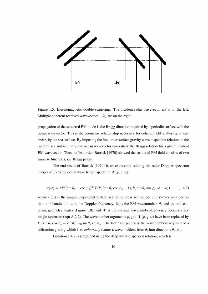
Figure 1.5: Electromagnetic double-scattering. The incident radar wavevector k0 is on the left.
Multiple coherent received wavevectors −k0 are on the right.
propagation of the scattered EM mode is the Bragg direction required by a periodic surface with the
ocean wavevector. This is the geometric relationship necessary for coherent EM scattering, to any
order, by the sea surface. By imposing the first order surface gravity wave dispersion relation on the
random sea surface, only one ocean wavevector can satisfy the Bragg relation for a given incident
EM wavevector. Thus, to first order, Barrick [1970] showed the scattered EM field consists of two
impulse functions, i.e. Bragg peaks.
The end result of Barrick [1970] is an expression relating the radar Doppler spectrum
energy σ(ω) to the ocean wave height spectrum W (p, q, ω):
σ(ω) = πk40(sin θs − cosϕs)
2W (k0(sin θs cosϕs − 1), k0 sin θs sinϕs, ω − ω0) (1.4.2)
where σ(ω) is the range-independent bistatic scattering cross section per unit surface area per ra-
dian s−1 bandwidth, ω is the Doppler frequency, k0 is the EM wavenumber, θs and ϕs are scat-
tering geometry angles (Figure 1.8), and W is the average wavenumber-frequency ocean surface
height spectrum (eqn A.2.2). The wavenumber arguments p, q to W (p, q, ω) have been replaced by
k0(sin θs cosφs − sin θi), k0 sin θs sinφs. The latter are precisely the wavenumbers required of a
diffraction grating which is to coherently scatter a wave incident from θi into directions θs, φs.
Equation 1.4.2 is simplified using the deep water dispersion relation, which is:
10

Figure 1.6: Second order hydrodynamic scattering. A nonlinear effect wherein two first order waves
[black] interact to produce a second order wave [red]. The second order waves are not a simple linear
superposition of first order waves. The wavevector geometry must satisy kB = k1 + k2, where
k1,2 are the first order waves and kB is the second order wave. Crestlines for the k1,2 wavefields
are shown in black, with kB shown in red. The second order crestlines connect points of k1,2
maximum constructive and destructive interference, i.e. crestline and trough intersects.
11

Figure 1.7: Hydrodynamic scattering. Same as Figure 1.6, with k1,k2 chosen to optimize the visual
Moire’ effect.
ω2g± = ±g
√p2 + q2 = ±g
√(am)2 + (an)2 (1.4.3)
The wavenumber-frequency spectrum then becomes:
W (p, q, ω) = 2W+(p, q)δ(ω + ω+) + 2W−(p, q)δ(ω + ω−) (1.4.4)
where the ± signs refer to the direction of motion of the waves. Substituting 1.4.4 into 1.4.2:
σ(ω) = 4πk40(sin θs − cosϕs)
2 [W+(p, q)δ(ω + ω+ − ω0)
+W−(p, q)δ(ω + ω− − ω0)] (1.4.5)
Note that the Doppler spectrum consists of two peaks centered at the carrier ω0 but shifted by an
amount:
ω± = ±√gk0(sin2 θs − 2 sin θs cosϕs + 1)1/2 (1.4.6)
12

Figure 1.8: from Barrick [1970]. Far-Zone scatter geometry. Square patch of side L, considerably
larger than the wavelength λ, but smaller than R0, the distance from the patch to the observation
point, i.e. λ << L << R0. ks0 is a unit vector pointing in the desired observation direction, i.e.
ks0 = sin θs cosφsx+ sin θs sinφsy + cos θsz.
13

These Doppler shifts correspond to the velocites of ocean waves with the proper lengths
for Bragg scatter, i.e. L = λ/(sin2 θs − 2 sin θs cosϕs + 1)1/2, where λ = 2π/k0 is the radio
wavelength. The frequency shift, ω±, is zero in the forward direction, where θs → π/2, ϕs → 0.
It is largest in the backscatter direction, where θs → π/2, ϕs → π. Here, ω± = ±√
2k0g, and
the lengths of the water waves responsible for scattering are the shortest, i.e. L = λ/2. The Bragg
wavevector will bisect the angle included between the Tx and Rx antennas (Fig 1.9).
Using the first order model, the shortest wavelength a radar can sample is the Bragg wave-
length, i.e. is controlled by the EM frequency (Eqn. 1.4.6). Longer wavelengths can be sampled
using bistatic Tx,Rx antenna separation, i.e. by varying the scattering angle ϕs. Barrick [1970,
sec. 4] discusses various bistatic radar configurations for employing the relationship between the
Doppler spectrum and the ocean waveheight directional spectrum (Eqn. 1.4.5). An example of
this is a bistatic surface-to-surface configuration using omnidirectional transmit and receive anten-
nas (Figure 1.9). A partially complete waveheight directional spectra could be generated using this
method and the assumption of a constant directional spectra across the measurement domain.
First order theory limits the explainable portion of the Doppler spectrum to the Bragg
peaks and the corresponding data to a one-dimensional sampling of the ocean wave directional
spectrum. As measurements show, there is a significant amount of coherent information throughout
the Doppler spectrum (Figure 1.1). Second order theory seeks to relate this region of the Doppler
spectrum to measurable properties of the ocean surface directional spectrum.
Hasselmann [1971] first suggested that the Doppler spectrum continuum resulted from
higher-order wave-wave interactions. According to this hypothesis, electromagnetic energy is scat-
tered by those combinations of interacting ocean waves that produce the required λ/2 periodicity on
the surface of the sea. Hasselmann based his analysis on a Feynman diagram formalization of the hy-
drodynamic effects [Hasselmann, 1966], but also included electromagnetic interaction. His analyis
predicted symmetrical sidebands on either side of the Bragg peaks, proportional to the waveheight
spectrum of the sea. The scattering equation of Barrick and Weber [1977] predicts non-symmetrical
sidebands, and multiple second-order peaks due to specific nonlinear wave interactions. It is the
prevailing theory in contemporary research, as it correctly predicts spectral characteristics found
in observations. Some early confirmation of the Barrick theory is in Tyler et al. [1972]. The the-
oretical second order Doppler spectrum of Derr [1972] is based on the Weber and Barrick [1977]
expressions for second order ocean gravity waves.
Weber and Barrick [1977] derived a more general solution to the nonlinear hydrodynamic
equations of motion for ocean waves by extending Stokes [1847] original perturbation analysis.
14

Figure 1.9: From Peterson et al. [1970]. Bistatic radar geometry. The geometrical figures are
ellipses, with foci at Point Arena and Sunset Beach, and circles which contain the chord line between
Point Arena and Sunset Beach.
15
Stokes’ solution was for a single gravity wave propagating with a rigid, periodic profile and a con-
stant velocity. Weber’s solution allows for a general periodic wave train, i.e. an arbitrary number
of distinct gravity wavevectors, with a non-rigid profile and different phase velocities. Weber and
Barrick [1977] applied the perturbation solution to find a second order correction to waveheight
and a third order dispersion relation correction. Barrick and Weber [1977] show that the general
two-dimensional solution [Weber and Barrick, 1977] agrees, within the appropriate limiting cases;
with Stokes [1847] for wave velocity and height correction for a single wave; with Longuet-Higgins
and Phillips’ 1962 phase velocity correction for one wave due to the presence of another colinear
wave; and with Tick’s 1959 result for the second-order waveheight of a one-dimensional wave train
profile.
An important result of Weber and Barrick [1977] is that the waveheights of various orders
do not all exist in the same wavevector-frequency domain (Eqn. A.6.3). In general, each order of
ocean waves has a different dispersion relation. By nature of the perturbation expansion, second
order waves are expressed as double products of first order wave height. Because the second order
waves cannot satisfy the first order dispersion equation, they are not ”free”, i.e. they do not remove
energy from the first order waves and cannot propagate freely without the existence of the two first
order waves. The analysis of Weber and Barrick [1977] has constraints to the domain over which
the solutions are valid. Energy transfer between waves, between the atmosphere and ocean, and
viscosity are neglected. The analysis represents the vertical displacement of the surface as a Fourier
series. Thus the spatial and temporal scales should be less than those over which energy transfer
processes are important, and large compared to the spatial periods 2π/k and temporal periods 2π/ω
of the dominant waves present.
The notationK,Ω is used for second order waves to indicate their exclusion from the first
order dispersion relation. The spatial wavenumber of the second order waveK is the vector sum of
the wavevectors of the first order waves present. The same is true for the frequencies.
K = k + k′ and Ω0 = ω0 + ω′0 (1.4.7)
(to lowest order, where ω0 =√gk and ω′0 =
√gk′).
Barrick and Weber [1977] explain Eqn. A.6.8 for the case of two first order sinusoidal
wave trains, where k,k′ = ±ka,±kb. There will be several second order wave trains whose
Fourier coefficients η2(K,Ω0) are determined by the products of terms in the sum. The four sets of
second order waves are:
16
1) The self effect (second harmonic) second order waves:
WavenumbersKaa = 2ka,Kbb = 2kb (1.4.8)
Frequencies Ω0aa = 2ω0a, Ω0bb = 2ω0b (1.4.9)
2) The mutual effect second order waves:
WavenumbersKs,d = ka ± kb (1.4.10)
Frequencies Ω0s,d = ω0a ± ω0b (1.4.11)
The analogy used by Barrick and Weber [1977] is Moire patterns in diffraction gratings
(Figure 1.7). The self effect waves are parallel to the first order waves, have half the spatial period of
the fundamental, but move at the same phase speed. Crestlines of the mutual effect waves connect
points of maximum constructive and destructive interference for first order waves, i.e. the first order
crest and trough intersects (Figure 1.6). In general, the self effect wave heights are of the same order
as the mutual effect waves. But as the number of first order waves N increases, the mutual effect
exceeds the self effect term, i.e. N vs. N(N − 1) ≈ N2 Barrick and Weber [1977]. The heights of
the second order waves are small compared to the first order waveheights, e.g. O(cm) second order
waves for O(m) first order waves Barrick and Weber [1977].
The gravity wave dispersion relation is expressed (to second order):
ω(k) = ω0 + ω2 = ω0(1 +ω2
ω0) =
√gk(1 +
ω2
ω0) (1.4.12)
and hence
vph =√gk(1 +
ω2
ω0) =
√gk(1 + ∆vph(k)) (1.4.13)
This correction term ω2/ω0 to the dispersion relation represents the correction to the phase
velocity of an ocean wave of length 2π/k. The form of A.6.10 indicates that the change in phase
velocity comes not only as a result of the existence of that wave alone, but as a result of the pres-
ence of all other waves [Barrick and Weber, 1977]; i.e. the aforementioned ”self” and ”mutual”
effects. Stokes [1847] analysis showed that the nonzero height of the original wave increases its
speed slightly, which agrees with the self effect term. The mutual effect term agrees with the anal-
ysis of Longuet-Higgins and Phillips [1962]. Barrick and Weber [1977] evaluated the phase speed
correction for two-wave interaction. In short, a longer, higher second wave produces a greater phase
17
velocity change on the first wave than a shorter, lower second wave. For parallel waves, the correc-
tion term has the same magnitude, but its sign is dependent on their relative directions. Orthogonal
incidence results in a phase speed increase, but the magnitude is relatively small compared with
parallel incidence (2.78% of the value for parallel incidence) [Barrick and Weber, 1977].
From Derr [1972] the expression for the second order Doppler spectrum in terms of the
ocean waveheight energy spectrum:
σvv(ωD) = 16πk40
∫ ∞−∞
∫ ∞−∞|ΓT (k1,k2)|2W (k1)W (k2)δ(ωD − ω1 − ω2)dpdq (1.4.14)
where σvv(ωD) is the average second order backscatter cross section per unit surface area per rad
s−1 bandwidth, k1 = (p − k0)x + qy, k2 = −(p + k0)x − qy, k1 = |k1|, k2 = |k2|, ω1 =
sgn(k1x)√
(gk1), ω2 = sgn(k2x)√
(gk2), η = ω − ω0 is the Doppler shift from the carrier, δ(x) is
the Dirac impulse function of argument x, and W (k) = W (kw, ky) is the directional waveheight
spectrum of the ocean. This equation is valid for backscattering at grazing incidence with vertical
polarization over a perfectly conducting sea.
The second order electromagnetic contribution ΓEM is found to be
ΓEM =1
2(k1xk2x − 2k1 · k2)/(
√k1 · k2 + k0∆) (1.4.15)
where ∆ is the normalized impedance of the sea surface.
The second order hydrodynamic effects produce:
ΓH = − i2
[k1 + k2 + (k1k2 − k1 · k2)(1− 2η2/(η2 − ω2
B))(g/ω1ω2)]
(1.4.16)
where i =√−1 and ωB =
√(2gk0) is the first order Bragg Doppler shift. The total Γ used in the
integral to account for both types of second order effects is Γ = ΓEM + ΓH .
Equation 1.4.14 shows that a double scatter Bragg process is responsible for the second
order Doppler spectrum. The scattered radio wavenumber−k0x is equal to k1+k2+k0x, where the
last term is the incident radio wavenumber. The frequency ω of the scattered field is ω1 + ω2 + ω0.
For EM second order effects, an ocean wavetrain with wavenumber k1 scatters the radio energy
along the surface to a second wavetrain with wavenumber k2, which redirects it back toward the
receiver (Fig 1.5); the intermediate radio wave can be either propagating or evanescent. For second
order hydrodynamic effects (Fig 1.6), two ocean wavetrains produce second order ocean waves with
wavevectors k1±k2; these latter ocean waves are not freely propagating because they do not satisfy
18
the first order gravity wave dispersion relationship [Derr, 1972]. One of the two integrals can be
done in closed form because of the Dirac function in the integrand. The remaining integration is
done numerically because of the complex form of the integrand.
The magnitude of the second order Doppler sidebands are dependent on sea state. These
sidebands contain continuous integrable singularities, i.e. spectral peaks, at Doppler frequencies√(2)fB and 23/4fB . The
√2 singularity is due to both electromagnetic and hydrodynamic second
order effects. The electromagnetic component is from ocean waves of length L = λ (rather than
λ/2). The hydrodynamic component is from a second spatial harmonic with length L = λ. The
23/4 singularity is due to a ”corner reflector” electromagnetic effect. This occurs when two sets of
first order scattering ocean waves pass through 45 with respect to the propagation direction [Derr,
1972].
The two-dimensional nonlinear integral equation 1.4.14 which gives the Doppler spec-
trum as a function of the directional ocean wave spectrum, [Barrick, 1970, Derr, 1972], is the core
equation used in further derivations of wave parameters. A further discussion of its properties is
given in §3.5.
1.5 Previous Research
High frequency ocean radar measures EM waves reflected from the ocean surface. This
signal results in a Doppler spectrum comprised of two large Bragg peaks and a continuum of second
order energy. Several ocean parameters can be inferred from this information; surface currents,
surface wind direction, vertical current shear, rms wave height, the scalar, and the directional ocean
wave spectrum.
1.5.1 Currents
The most robust radar-derived estimate is surface current velocities. Surface currents
within the orbital depth decay of the ocean Bragg waves will modify their apparent celerity. This
additional celerity is measured as a difference from the expected Doppler shift in the radar spectrum.
The success of this method lies in its simplicity and direct relationship to the received signal. The
strongest feature of the Doppler spectrum are the Bragg peaks, typically at 20-30 dB above the
second-order continuum (Heron and Heron, 1998). Furthermore, only the frequency location of the
Bragg peaks is required, whereas phase and amplitude are relatively more sensitive to internal and
19
external noise sources. Methods for extracting the frequency of the first order peaks are discussed
in §2.2.
This method has been widely used to map sea surface currents and investigate physical in-
teractions. Stewart and Joy [1974] used a multifrequency radar on San Clemente Island to measure
the vertical current shear at two bearings. Heron et al. [1985] operated a narrow-beam radar inside
the Great Barrier Reef, achieving 5 cm s−1 accuracy. OSCR-derived tidal currents have been com-
pared to near-surface current measurements [Prandle, 1987] and modeled velocities [Prandle and
Ryder, 1989]. Statistical analysis found the standard error of OSCR to be less than 4 cm s−1. Shay
et al. [1995] compared radar currents to subsurface ultrasonic current meters. Regression analysis
indicated a bias of 2-4 cm s−1 and slope of O(1), with periods of high and low correlation. Graber
et al. [1996] compared OSCR currents to interferometric synthetic aperture radar INSAR, shipboard
measurements, and buoys. Kosro et al. [1997] found OSCR and ADCP currents with correlations of
∼ 0.8 and rms differences of ∼ 15 cm s−1. Shay [1997] found radar current oscillations within the
internal wave continuum from the buoyancy to the inertial frequencies. Chavanne et al. [2007] com-
pared tidal currents in the Adriatic Sea to model results, and investigated the interactions between
mesoscale currents and internal tides [Chavanne, 2007].
A relatively new development is the measurement of vertical current shear via radar
[Shrira et al., 2001]. They demonstrate the ability to measure depth integrated currents to three dif-
ferent depths; employing the known ocean wavevectors of the second order singularities, i.e. 21/2fB
and 23/4fB second harmonics and corner reflections, in conjunction with the Bragg wavevector.
1.5.2 Winds
The surface wind direction can be inferred from radar spectra. The method for estimating
wind direction from radar spectra was originally developed by Long and Trizna [1973] for use
with skywave radar. The experiment was conducted at the U.S. Naval Research Laboratory, and
generated wind maps for large areas of the Atlantic. Stewart and Barnum [1975] evaluated the
accuracy of that technique. The wind direction method of Long and Trizna [1973] has since been
applied with success to ground wave HF radar.
The Long and Trizna [1973] method is as follows: If the wind has remained constant over
enough time and fetch, the surface wave energy will be in equilibrium with the wind, and can be
modeled as a 2-dimensional cardiod distribution as a function of angle with respect to wind direction
[Longuet-Higgins et al., 1963]. Longuet-Higgins et al. [1963] suggested the form:
20

G(θ) = A coss(θ/2) (1.5.1)
where G(θ) represents the angular distribution of wave energy, A is a constant, θ is the angle from
the direction of maximum wave energy, i.e. the angle of the wind, and s is a spreading parameter.
A is a constant required for the normalization∫ π−π A coss(θ/2)dθ = 1 for different values of s.
The Bragg ratio RB is defined as the ratio of energy in the approaching to receding Bragg
peak [Long and Trizna, 1973]. Bragg peaks with a positive Doppler shift are due to waves ap-
proaching the radar, whereas the negative Bragg peak is due to receding waves. The magnitude of
the Bragg peak is directly related to the energy within the approaching and receding Bragg waves
(Figure 1.10). Following Fernandez et al. [1997] the Bragg ratio is:
RB = B+/B− (1.5.2)
where B+ and B− are the positive and negative Bragg peaks, respectively. If the wind vector is
directed towards the radar, the majority of the Bragg waves will be propagating towards the radar,
causing the Bragg ratio to be positive and large. If the wind vector is perpendicular to the radar
direction, then B+ ∼ B−, and the Bragg ratio will be near zero.
Define θ+ and θ− as the angles between the wind vector and the approaching and receding
Bragg waves, respectively. Substituting the cardiod distribution of 1.5.1 into 1.5.2 yields:
RB =coss( θ
−−180
2 )
coss(θ−/2)= tans(θ−/2) (1.5.3)
There is a left-right ambiguity in 1.5.3 that can be resolved using observations from two radar
stations. Equation 1.5.3 can be inverted for θ− if a value for s is assumed; θ− = 2 arctan(R1/sB )
Two fundamental assumptions allow for inference of surface wind direction from radar
spectra. The first is that the Bragg waves are locally generated by the wind. That is, a stationarity in
space and time is assumed. Bragg wave propagation and evolution as a function of wind history and
outside energy sources is not considered. The method of Long and Trizna [1973] assumes the ocean
Bragg wave energy are proportional to the spectral power of the Bragg peaks, following Barrick
[1970]. This implies a 1:1 instantaneous mapping of wind direction to Bragg wave amplitude and
direction. The second assumption is a priori knowledge of the Bragg wave directional spreading
function. The accuracy of radar-derived wind direction estimates depends on the model used, spatial
and temporal variability in the measurement cell, the GDOP, antenna beamforming, and noise levels.
The accuracy of the stationarity assumption is largely dependent on the Bragg wavelength.
Ocean waves of different wavelengths respond differently to changes in wind speed and direction.
21

Figure 1.10: From Fernandez et al. [1997]. Sample distributions of surface wave energy as a func-
tion of angle relative to the wind direction for cases with wind blowing toward (left), at right angles
to (middle), and away from (right) the radar look direction. Sample backscatter spectra below show
relative heights of the approaching (+) and receding (-) Bragg peaks for each case and θ+ denotes
the angle between the wind and the approaching wave directions.
22

Figure 1.11: From Harlan and Georges [1994]. Comparison of several semiempirical models for
the dependence of the Bragg ratio RB on wind direction, measured from the radar look direction.
LT indicates the Long and Trizna [1973] model. SB2 and SB4 indicate the Stewart and Barnum
[1975] model with s = 2, 4 for the spreading function
To assume local generation, the Bragg waves must be significantly damped before entering the next
grid cell, and they must quickly reach equilibrium with a turning surface wind. Masson [1990]
studied directional wave spectra during turning wind events, and estimated relaxation coefficients
as a function of wave frequency. van Vledder and Holthuijsen [1993] give equations for calculating
the Bragg wave group speed and damping rate. Thus energy propagation between range cells,
and response time for shifting winds can be evaluated. For example, Harlan and Georges [1994]
calculated a 36 min response time for 10 m Bragg waves under an 8 m s−1 wind.
The exact form of the directional spreading function is unkown, and observations indicate
that a specific functional form is difficult to justify [Phillips, 1966, Nierenberg and Munk, 1969].
Assumptions of unimodality or symmetry are not valid [Masson, 1990]. Higher wind speeds pro-
duce more directional spreading [Stewart and Barnum, 1975]. At low wind speeds, directional
variability complicates measurement Pierson Jr. [1990] and Gilhousen [1987]. For a given Bragg
ratio, the estimated wind direction can vary by 30 depending on the choice of spreading model
(Figure 1.11). The reader is referred to Banner and Young [1993] for an evaluation of wind-wave
models, and Harlan and Georges [1994], Wyatt [2001] for their application to radar measurements.
23
Donelan et al. [1985] conducted a detailed study of deep water wind-wave evolution using
an array of 14 wave gauges. They proposed a directional spreading function near the spectral peak
of:
D(θ, k) = sech2 β(θ − θw) (1.5.4)
where k is the wavenumber, θ is the polar direction, and θw is the wind direction. They found
the primary variation of β was on k/kp, where kp is the wavenumber of the spectral peak. At
frequencies above 1.6fp, the directional spread becomes noisy.
Maresca and Georges [1980] used a coss(θ/2) spreading model, and found less accurate
results for large s, i.e. highly directional wave distributions. Harlan and Georges [1994] identified
an operational limitation wherein the measurable Bragg ratio did not exceed a maximum value,
i.e. an upper limit to the directionality of the spreading function. This was also noted by Gurgel
et al. [2006]; observed ratios did not exceed±20 dB, corresponding to an inability to measure wave
directions between ±15 or ±165 degrees (the chosen coss model requires a peak Bragg ratio of
±25 dB). Wyatt [2001] proposed using the Donelan et al. [1985] sech2 β(θ) model, as it does not
give infinite values for angles near 0 or 180. It can be adjusted to give the same slope as the coss
model with β = 0.7 or to cover the observed Bragg ratios of± ≈ 20 dB with β = 1.0. Gurgel et al.
[2006] found the best fit to buoy measurements with β = 0.8.
Numerous studies have compared radar-derived wind direction estimates to alternative
measurements. [Stewart and Barnum, 1975] found the Bragg ratio method accurate to within 16
compared to shipboard anemometer measurements. Using the same WARF radar, Maresca and
Georges [1980] found wind direction agreement of 7 compared to a National Data Buoy Office
(NDBO) buoy. Shearman and Wyatt [1982] describe the results of mapping winds during the JASIN
experiment. Heron et al. [1985] found agreement of ±10 within a swell-shadowed region of the
Great Barrier Reef using in-situ measurements. Using a OTH radar, Harlan and Georges [1994]
accurately recreated ocean-basin scale wind fields (18 · 106 km2) using an empirical fit to NMC
model and buoy data, yielding a rms error of ∼ 33 (Figure 1.12). Fernandez et al. [1997], Wyatt
[1997] compared wind direction estimates obtained from the OSCR radar at the DUCK facility to
offshore moored buoys and a research pier station (Figure 1.13). Spatial maps of wind direction
have shown variations over horizontal scales of a few kilometers, and resolved the passage of a
sharp front [Fernandez et al., 1997].
Vesecky et al. [2002] used a partial least squares (PLS) method combined with in-situ
measurements to add magnitude to wind estimates from a multifrequency radar. This is a unique
24

Figure 1.12: From Harlan and Georges [1994]. 1900 OTH radar measurements of the Bragg ratio
RB plotted against the magnitude of the NMC or in situ wind direction, measured relative to the
direction of arrival of the radar ray. Each radar measurement falls within 100 km and 1.5 hours of
the corresponding model or in-situ measurement. The correlation coefficient is 0.69.
addition to the Long and Trizna [1973] method which cannot infer wind magnitude. The PLS
technique uses linear regression to fit observations to a statistical model, and achieved a standard
error of prediction of ∼ 40 and r2 =∼ 0.45.
1.5.3 Waves
Using electromagnetic and hydrodynamic theory, Barrick [1977] derived an integral ex-
pression for the root-mean-square waveheight (hereafter Hs) as a function of the Doppler spectrum:
Hs2 =
2∫∞−∞ σ2(ωd)/W (ν)dωd
k20
∫∞−∞ σ1(ωd)dωd
(1.5.5)
W (ν) =8
k20
|Γ|2 (1.5.6)
where ν = ωd/ωB is Doppler frequency normalized to the Bragg frequency. σ1 is the first order
power (integrated power spectral density), σ2 is the second order power, ωd is the Doppler shift
frequency (Hz), ωB is the Bragg frequency (Hz), k0 is the incident EM wavenumber (rad/m), and
W is a dimensionless weighting function. The total coupling coefficient Γ is defined in Equations
25

Figure 1.13: From Fernandez et al. [1997]. Wind direction relative to the master radar site measured
at a wave buoy off Duck, North Carolina in October 1994 (solid) together with estimates from the
HF radar (symbols) for a 2-day period.
26
1.4.15,1.4.16. The assumption of a mean weighting function |Γ|2 over all directions allows 1.5.5 to
be independent of direction, and thus Hs can be estimated from the radar spectrum alone, without
a-priori knowledge of the sea state. Estimation of the first and second order powers σ1,σ2 from the
measured Doppler spectrum is discussed at length in subsequent sections.
There are three sources for error in the radar-derived Hs estimate. They include; theo-
retical error, statistical i.e. sampling error, and noise. The first two can be calculated, whereas
noise error can only be identified and avoided. Theoretical error arises from use of the EM scat-
tering equations and their inherent inaccuracies and limitations. Theoretical analysis herein will be
limited to the Hs equation 1.5.5. For inter-comparison of various radars the relative standard error
(RSE), i.e. the standard deviation of the measurements normalized by the mean, will be referred to.
This compensates for increased measurement variation due to greater waveheights.
There are three limitations to the mathematical validity of the EM scattering equations
[Barrick, 1970]. 1) Small amplitude approximation: the sea surface height ζ above the mean plane
is small in terms of the EM wavelength. 2) Small slope approximation: the sea surface slope ∇ζ is
small. 3) The medium is highly conducting. Conditions (1) and (3) are not a concern for HF radar.
The shortest wavelength for HF is ∼ 10 m, thus the small amplitude (1) approximation is satisfied.
Sea water satisfies (3) below UHF (300 MHz). Condition (2) is a documented limitation, often
referred to as the ”saturation limit”, wherein large waveheights cause the second order continuum
to be indistinguishable from the first order Bragg peaks [Lipa and Nyden, 2005]. The small slope
assumption requires k0Hs < 4. Wyatt et al. [1999] noted an upper limit of Hs = 7.1 m for a 27.65
MHz radar, i.e. k0Hs = 4.11. The empirical method of Gurgel et al. [2006] failed near this limit,
due to spectral merging of the first and second order regions. The saturation limit is not only a
mathematical limitation, but a physical limitation to radar operation.
Barrick [1977] tested 1.5.5 using the Phillips [1966] synthetic wave model, and concluded
the formulas were only weakly dependent on the incident radar-wave direction, above a certain
k0Hs limit. Synthetic testing showed poor accuracy below k0Hs < 0.1, indicating a theoretical
limit. Above k0Hs > 0.3, RSE for Hs was 22.7% [Barrick, 1977]. Observations of a 7-10 MHz
radar operating over a 10 month period yielded poor accuracies below 1 m Hs [Wyatt et al., 2006].
This corresponds well to the lower theoretical limit of 0.7 m.
Maresca and Georges [1980] investigated two semi-empirical methods for estimating
wave parameters from the radar data; the rms waveheight Hs, and the scalar wave spectrum. Both
methods involved generating a range of synthetic ocean wave directional spectra, passing them as
inputs to the second-order EM scattering model of Weber and Barrick [1977] (Eqn. A.6.17), and
27
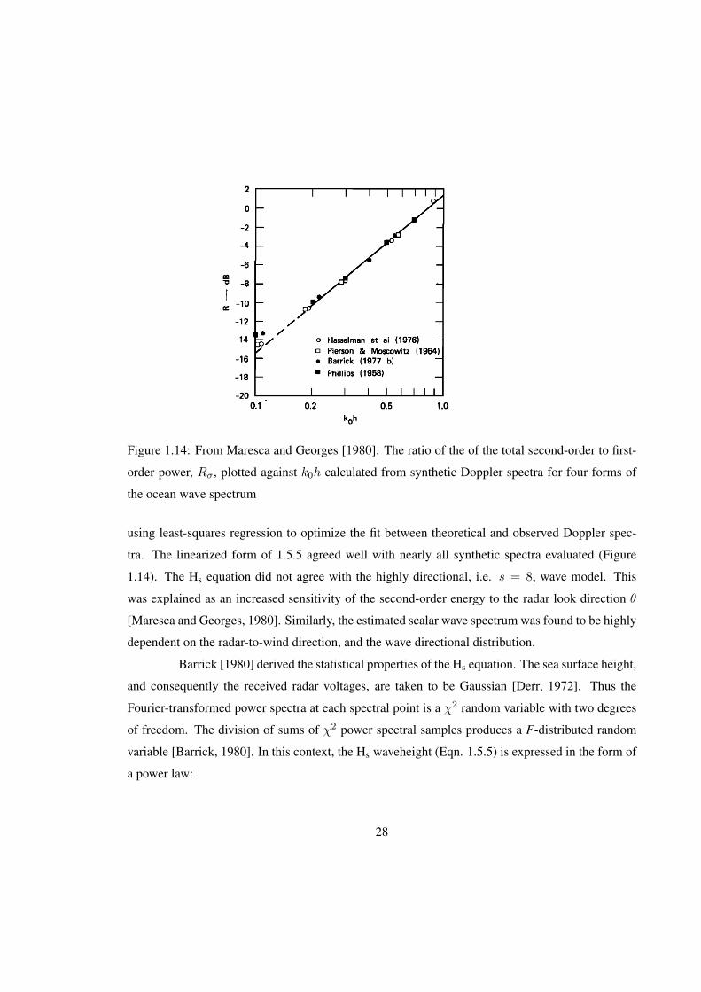
Figure 1.14: From Maresca and Georges [1980]. The ratio of the of the total second-order to first-
order power, Rσ, plotted against k0h calculated from synthetic Doppler spectra for four forms of
the ocean wave spectrum
using least-squares regression to optimize the fit between theoretical and observed Doppler spec-
tra. The linearized form of 1.5.5 agreed well with nearly all synthetic spectra evaluated (Figure
1.14). The Hs equation did not agree with the highly directional, i.e. s = 8, wave model. This
was explained as an increased sensitivity of the second-order energy to the radar look direction θ
[Maresca and Georges, 1980]. Similarly, the estimated scalar wave spectrum was found to be highly
dependent on the radar-to-wind direction, and the wave directional distribution.
Barrick [1980] derived the statistical properties of the Hs equation. The sea surface height,
and consequently the received radar voltages, are taken to be Gaussian [Derr, 1972]. Thus the
Fourier-transformed power spectra at each spectral point is a χ2 random variable with two degrees
of freedom. The division of sums of χ2 power spectral samples produces a F-distributed random
variable [Barrick, 1980]. In this context, the Hs waveheight (Eqn. 1.5.5) is expressed in the form of
a power law:
28
k0Hs = Cqp (1.5.7)
where k0 is the radar wavenumber, C is a constant, q is the quotient of spectral sums, i.e. second or-
der to first order energy, and p is by theory 1/2. By the aforementioned argument, q is F-distributed.
For a radar which collects K sequential spectra in time at a fixed range, the best possible
accuracy is obtained by simply averaging all K spectra Barrick [1980]. It makes no difference how
the timeseries are divided into individual spectra. The situation becomes more complicated when
one desires to average consecutive spectra in range or time, as individual spectra will have varying
path loss and system gain, i.e. signal-to-noise ratios. These gain factors must be removed prior to
averaging, via the second-to-first order energy quotient q.
The obvious method is to average the quotients q for each power spectrum, as this cancels
the variable gain factors; k0h = C〈q〉p. But for 0 < p < 1, both the error and bias are improved
by averaging the quotient to its pth power; k0h = C〈qp〉 [Barrick, 1980]. Furthermore, when the
denominator of q has many samples N , the standard deviation of q improves [Barrick, 1980]. This
is not the case for the Hs calculation, as relatively few Bragg peak spectral points comprise the
denominator. By averaging the reciprocated quotient q−1, the error improves. Thus, the RSE and
bias are minimized by averaging the reciprocated quotient to the pth, i.e.
k0h = C〈q−p〉−1 (1.5.8)
The normalized standard deviation σ, i.e. RSE, and waveheight bias hb/h due to sampling are given
as:
σ(h) = σ(q−p)/(⟨q−p⟩2√
K) (1.5.9)
hb/h =⟨q−p⟩−1 (1.5.10)
where K is the number of spectra averaged together, hb is the calculated Hs, and h is the true Hs.
In summary, the best Hs accuracy is achieved by simply averaging equal-gain spectra.
For unequal-gain spectra the gain must be eliminated via a normalization, e.g. quotient, prior to
averaging. In this case, accuracy always increases by having more samples, i.e. higher frequency
resolution, i.e. no incoherent averaging of spectra [Barrick, 1980].
Multiple researchers have reported on observed error in radar Hs measurements (Table
1.1). Using a 20 kW skywave radar, Maresca and Georges [1980] compared radar Hs to a National
Data Buoy Office buoy for waveheights of 0.3-0.8 m. Using eqn. 1.5.9, they calculated Hs RSE
29

of 3.3% compared to observations of ∼ 15% (N=84). They attributed the primary difference to a
lack of normalization prior to spectral averaging, i.e. compensating for path gains. Heron et al.
[1985] compared a 30 MHz ground wave radar to a Datawell waverider buoy within the Great Bar-
rier Reef for a 24 hour period. Root-mean-square deviations were 0.15 m for 0-1 m waveheights.
Deviations at these low waveheights were attributed to noise in the second order part of the Doppler
spectrum. Heron et al. [1998] compared the OSCR radar to a NOAA directional wave buoy. Radar
measurements were averaged over 20 km2 corresponding to N=15 individual spectra. RSE was
∼ 20% for observed waveheights of 0-1 m, with a correlation of 0.97. Using a unique algorithm
method, Essen et al. [1999] compared the WERA radar to 34 days of directional waverider buoy
data. Measures of first order variance were highly correlated (r= 0.8-0.9) for some regions of the
spatial field. Good data was obtained to a range of 30 km, with some degradation due to exter-
nal noise. Caires [2000] reported decreased accuracies for the OSCR radar away from the center
of measurement region. Compiling data from the Eurorose, SCAWVEX, and SHOWEX experi-
ments, Wyatt and Green [2002] reported a mean correlation coefficient of 0.94 between radar and
buoy measurements for the PISCES and WERA radars, and a RSE of 10.5% (N=9169). The main
limitations to Hs accuracy were scattering theory, noise sources, and antenna sidelobes [Wyatt and
Green, 2002]. It was further noted that strong, directional external noise in the daytime decreased
spatial coverage across all directions. Wyatt et al. [2003] compared the WERA and WaMoS radars
to waverider buoys at 3 different locations, and to the WAM model. Hs waveheights ranged from
1-8 m. The WERA had a mean correlation of 0.94 to the buoys, and a mean RSE of 16.6%. Wyatt
et al. [2005] evaluated the OSCR radar with two buoys and concluded the dataset was unsuitable for
wave measurements, despite a mean Hs correlation coefficient of 0.88. Primary limitations were the
OSCR hardware, deployment configuration, poor beamforming, and signal to noise ratios. Wyatt
et al. [2006] reported on 10 months of operational data from the PISCES radar. The lower operating
frequencies of 7-10 MHz combined with high transmit power (up to 1.2 kW) allows the PISCES to
achieve wave measurements up to ranges of 120 km. A useful lower limit of 2 m Hs was noted for
radar wave measurements, attributed to the longer Bragg waves.
30

Table 1.1: Comparison studies of radar to buoys
Observedradar λB (m) Hs(m) Correlation σ
Maresca and Georges [1980] WARF* 9-15 0.3-0.8 7,17%Heron et al. [1985] COSRAD 5 0-1 > 15%Heron et al. [1998] OSCR 6 0-1 0.97 20%Wyatt and Green [2002] PISCES,WERA 6-15,10-25 0.5-4 0.94 10.5%Wyatt et al. [2003] WERA 1-8 0.94 16.6%Wyatt et al. [2005] OSCR 0.5-3 0.88Wyatt et al. [2006] PISCES 15-21 0.5-8 0.90 33.8%λB: Bragg wavelength, σ: normalized standard deviation, i.e. relative standard error* skywave radar
31

Chapter 2
Methods
2.1 WERA radar and directional wave buoy
The reference data set for this study comes from a Datawell MarkIII directional wa-
verider buoy. Data were furnished by the Coastal Data Information Program (CDIP), Integrative
Oceanography Division, operated by the Scripps Institution of Oceanography. According to the
manufacturer, the buoy is accurate to 0.5% of the measured waveheight value. The buoy is located
approximately 4.3 nm west of Sunset Point, Oahu, Hawaii, and is hereafter referred to as the CDIP
buoy. Archived ocean wave parameters include scalar spectral energy, directional Fourier coeffi-
cients, significant wave height Hm0 from the zeroth moment of the energy spectrum, peak period
Tp, mean direction at the peak period Dp, and the average period Ta (m0/m1 spectral moments).
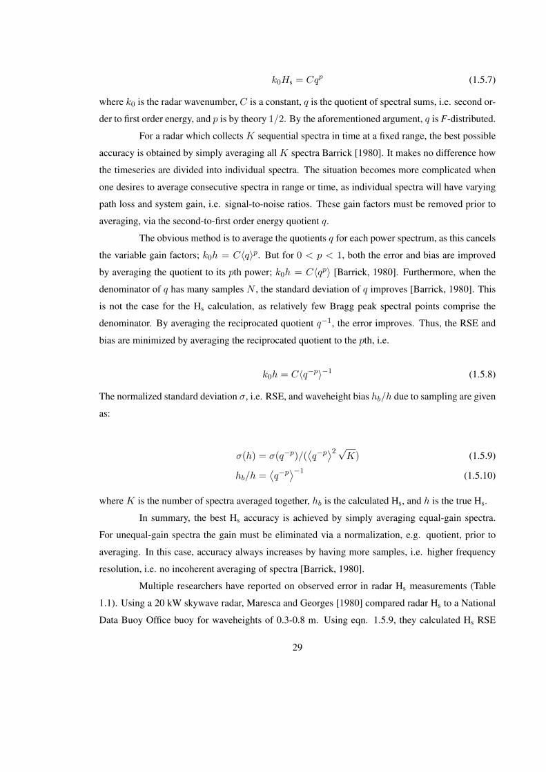
The buoy spectra are from a 2048 point timeseries at 1.28 Hz, incoherently averaged to a 64-point
spectra with variable bandwidth (Figure 2.1). Using the Maximum Entropy Method (MEM) [Lygre
and Krogstad, 1986], the directional Fourier coefficients and energy spectra were used to generate
directional spectra (Figure 2.2).
The radar data set used for this study was collected during the Hawaiian Ocean Mix-
ing Experiment (HOME) between 2000 and 2002. The instrument used was the HF Wellen radar
(WERA), developed at the University of Hamburg. Two radar sites were employed near the extreme
North-South points of the western coast (Figure 2.3). The northern site was located at the top of the
Waianae mountain range near Kaena Point. The southern site was located near the Koolina Resort.
Hereafter the sites will be referred to as Kaena and Koolina. The WERA operated at a transmit
frequency of 16.046 MHz, 102.5 km maximum range, 1.5 km range resolution, and 7.2 degree an-
gular resolution. Corresponding to this operating frequency, the Bragg scattering waves are 9.38 m
wavelength, wavenumber k0 = 0.67 rad s−1, with 2.45 s period. The data was interpolated from a
32
0 0.1 0.2 0.3 0.4 0.5 0.610
−6
10−5
10−4
10−3
10−2
10−1
100
101
102
Hz
Pow
er
Spectr
al D
ensity m
2/H
z
z raw
z, smoothed
CDIP Energy Density
Figure 2.1: An example spectrum from the Waimea CDIP buoy. Incoherent averaging of the raw
spectra [black] is used to improve the SNR of the data product [blue], at the cost of reduced fre-
quency resolution. Similar results are achieved using a Hamming window [pink].
33

Figure 2.2: An example directional spectrum from the Waimea CDIP buoy. The polar plot is aligned
with True North, with frequency increasing radially. Energies are indicated in the direction they are
propagating towards, i.e. the peak energy at 135 is moving south-east [black line].
34

Figure 2.3: Radar site geometry for the HOME experiment. The two radar sites are indicated in
blue. Both sites sampled 120 arcs, with ∼ 60 of overlap. Range arcs are shown at 50 and 100
km. The polar data was interpolated to a cartesian grid with 2 km resolution [dots]. The mean swell
direction for this study was 150 degrees [arrow].
polar to cartesian coordinate system with 2 km resolution in the horizontal and vertical, with 80x90
sample points respectively (Figure 2.3).
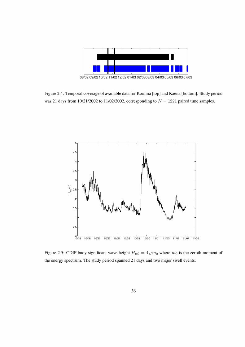
A relatively short 21-day subset of the available data was chosen for analysis. This period
coincides with previous research of tidal and mesoscale currents [Chavanne et al., 2007, Chavanne,
2007] using the same data set. Both radar stations were operational during this period, correspond-
ing to 1221 paired time samples (Figure 2.4). Two large swell events occurred during the study
period (Figure 2.5).
35
08/02 09/02 10/02 11/02 12/02 01/03 02/0303/03 04/03 05/03 06/03 07/03
Figure 2.4: Temporal coverage of available data for Koolina [top] and Kaena [bottom]. Study period
was 21 days from 10/21/2002 to 11/02/2002, corresponding to N = 1221 paired time samples.
Figure 2.5: CDIP buoy significant wave height Hm0 = 4√m0 where m0 is the zeroth moment of
the energy spectrum. The study period spanned 21 days and two major swell events.
36
2.2 Processing
The raw data created by a HF radar is not simply or directly related to the physical pro-
cesses measured. Algorithms are used to process the raw data into ocean state parameters. The
primary tasks of an oceanographic radar algorithm are the identification and delineation of Doppler
features, combined with some degree of quality control. The spectral peaks are not fixed in fre-
quency location, necessitating search and delineation functions. Filtering and averaging in both
space and time are usually employed. Data-adaptive or fixed parameter methods may be used.
Quality control logic for the inclusion or rejection of data can be based on different criteria. These
tasks are held in contrast to the well defined and unambiguous equations relating Doppler features
to ocean parameters. The algorithmic technique by which the tasks are accomplished, and with
varying skill, is arbitrary and thus a potential source of error.
The WERA radar is paired with a scientific analysis package, hereafter referred to as the
WERA algorithm. As explained in §3, initial evaluation of WERA Hs error motivated stepwise in-
spection of the processing algorithm. Since the intermediate WERA variables were not available, a
similar algorithm was developed for this work, hereafter the GS algorithm. Differences between the
algorithms will be discussed with regard to effects on the final data products. When the algorithms
are not mentioned, it is implied they are either identical in method or not significantly different in
analysis. A summary of the WERA algorithm is given in §B.
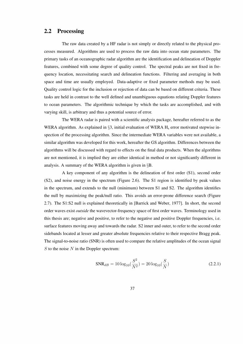
A key component of any algorithm is the delineation of first order (S1), second order
(S2), and noise energy in the spectrum (Figure 2.6). The S1 region is identified by peak values
in the spectrum, and extends to the null (minimum) between S1 and S2. The algorithm identifies
the null by maximizing the peak/null ratio. This avoids an error-prone difference search (Figure
2.7). The S1:S2 null is explained theoretically in [Barrick and Weber, 1977]. In short, the second
order waves exist outside the wavevector-frequency space of first order waves. Terminology used in
this thesis are; negative and positive, to refer to the negative and positive Doppler frequencies, i.e.
surface features moving away and towards the radar. S2 inner and outer, to refer to the second order
sidebands located at lesser and greater absolute frequencies relative to their respective Bragg peak.
The signal-to-noise ratio (SNR) is often used to compare the relative amplitudes of the ocean signal
S to the noise N in the Doppler spectrum:
SNRdB = 10 log10(S2
N2) = 20 log10(
S
N) (2.2.1)
37
Figure 2.6: An example Doppler spectra from Kaena. First order (S1) region is in red. Second order
(S2) region in blue. The frequency location of the S1:S2 null delineates the two regions. Noise level
is ∼ −45 dB
where S is the amplitude of a signal sinusoid. A decibel scale is used because of the large dynamic
range.
Proceeding the delineation of the first and second order regions, the centroid frequency of
the Bragg peak can be calculated. Accurate estimation of the Bragg peak frequency is necessary for
calculation of surface currents, and it is also required for second order measurements. The Doppler
shift due to surface currents must be removed from the spectra before further averaging or inter-
comparison. The simplest estimate is the frequency of the peak spectral value. A more physically
sensible alternative is the centroid frequency, as it is the mean location of signal energy [Barrick,
1980]. The definition of centroid frequency is:
f =∆f
∑iPi∑Pi
(2.2.2)
38

Figure 2.7: Hs errors due to a difference search in the S1:S2 null detection. Difference searches
tend to amplify noise. In this example, S1 energy is being underestimated due to slope inversions in
the Bragg peak, i.e. ”split peaks”.
where ∆f is the spectral frequency resolution, i∆f is the frequency position of the ith point, and Pi
is the spectral power at point i. Barrick [1980] derived a general expression for the error in centroid
frequency as the standard deviation of f − ft where ft is the true position of the peak:
σ(f − ft
∆f) =
√1K
∑i i
2P 2i∑
i Pi(2.2.3)
For the centroid equation 2.2.2, Barrick shows that it makes no difference in accuracy how the
original fixed length time series is divided into consecutive spectra and incoherently averaged. To
decrease the centroid frequency standard deviation by a factor of two, the time series length must
be increased by a factor of four.
Both the WERA and GS algorithm use the centroid method for estimating the Bragg
peak frequency location. The GS algorithm had consistent results for SNR > 10 dB (Figure 2.8).
Centroid frequencies result in greater radial current resolution, as they use 1/N∆f compared to
1/∆f for a simple Bragg peak maximum (Figure 2.9). The accuracy of the two frequency location
estimates cannot be evaluated without a reference measurement. The frequency difference between
the two methods is Gaussian distributed with zero mean, and tails off (3σ) at ∼ 1∆f (Figure 2.10),
suggesting the centroid calculation is not a significant source for processing error.
39

Figure 2.8: Results from the Bragg centroid frequency algorithm for a single time frame. The
underlying image is a spectrogram of power spectral density with frequency on the horizontal axis
and range on the vertical. Frequency locations of the Bragg peaks are marked for each range cell
[magenta].
40
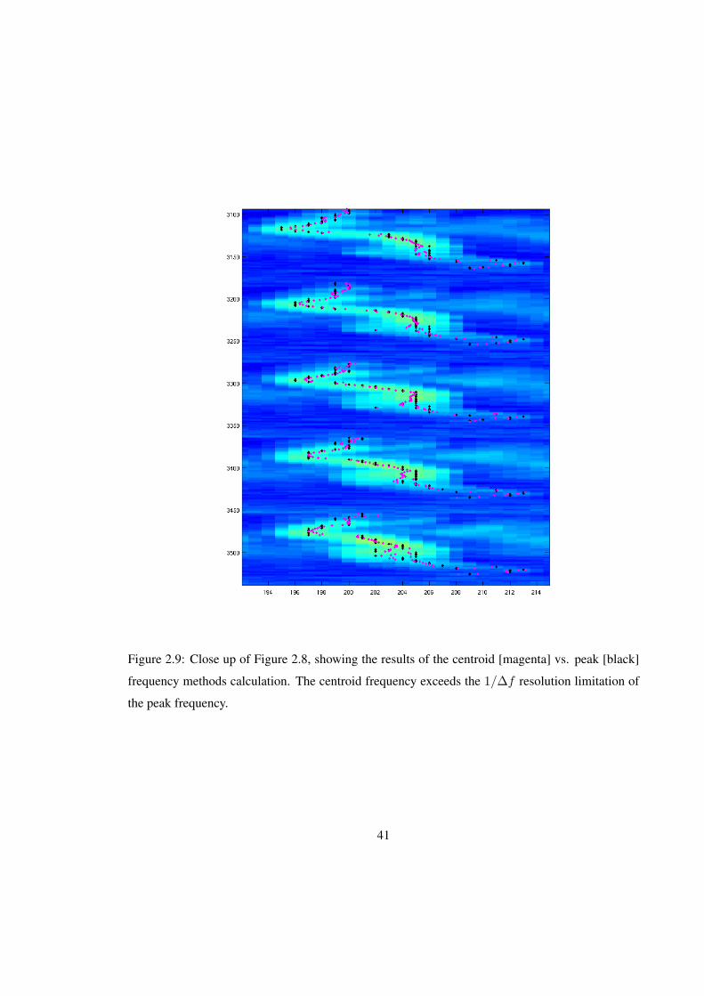
Figure 2.9: Close up of Figure 2.8, showing the results of the centroid [magenta] vs. peak [black]
frequency methods calculation. The centroid frequency exceeds the 1/∆f resolution limitation of
the peak frequency.
41

Figure 2.10: The distribution of frequency difference for Bragg frequency methods is Gaussian-like
with (±3σ) at ∼ 1∆f . Units on both plots are ∆f . The spatial field of the difference is plotted on
the right.
42

Chapter 3
Results
3.1 Winds
QuickSCAT and Multi-Spectral Model (MSM) wind model output was obtained for com-
parison to the radar wind fields(Figure 3.1). A composite field of MSM and RSM data was re-
sampled to match the WERA processing grid, hereafter RMSM. QuickSCAT spatial resolution was
much coarser (Figure 3.2), with ¡ 10 spatial samples available for a given time.
Inspection of the wind estimates from the Oahu radars showed good spatial and temporal
coherence (Figure 3.3), with significantly more spatial variance than the RMSM data (Figure 3.4).
The O(1000) data points from the RMSM field could essentially be reduced to a single wind vector
with little loss of information. Maximum vector correlation between the RMSM and radar fields
was r2 = 0.23.
The radar winds were binned into an angular histogram as a function of time and com-
pared to the mean QuickSCAT wind direction (Figure 3.5). Strong agreement between the radar
wind fields and QuickSCAT samples was found. Complex correlation between the mean radar and
QuickSCAT wind timeseries was r2 = 0.83, with zero angular bias. The radar wind histogram
revealed bimodal wind fields not observed in the reference data sets.
43
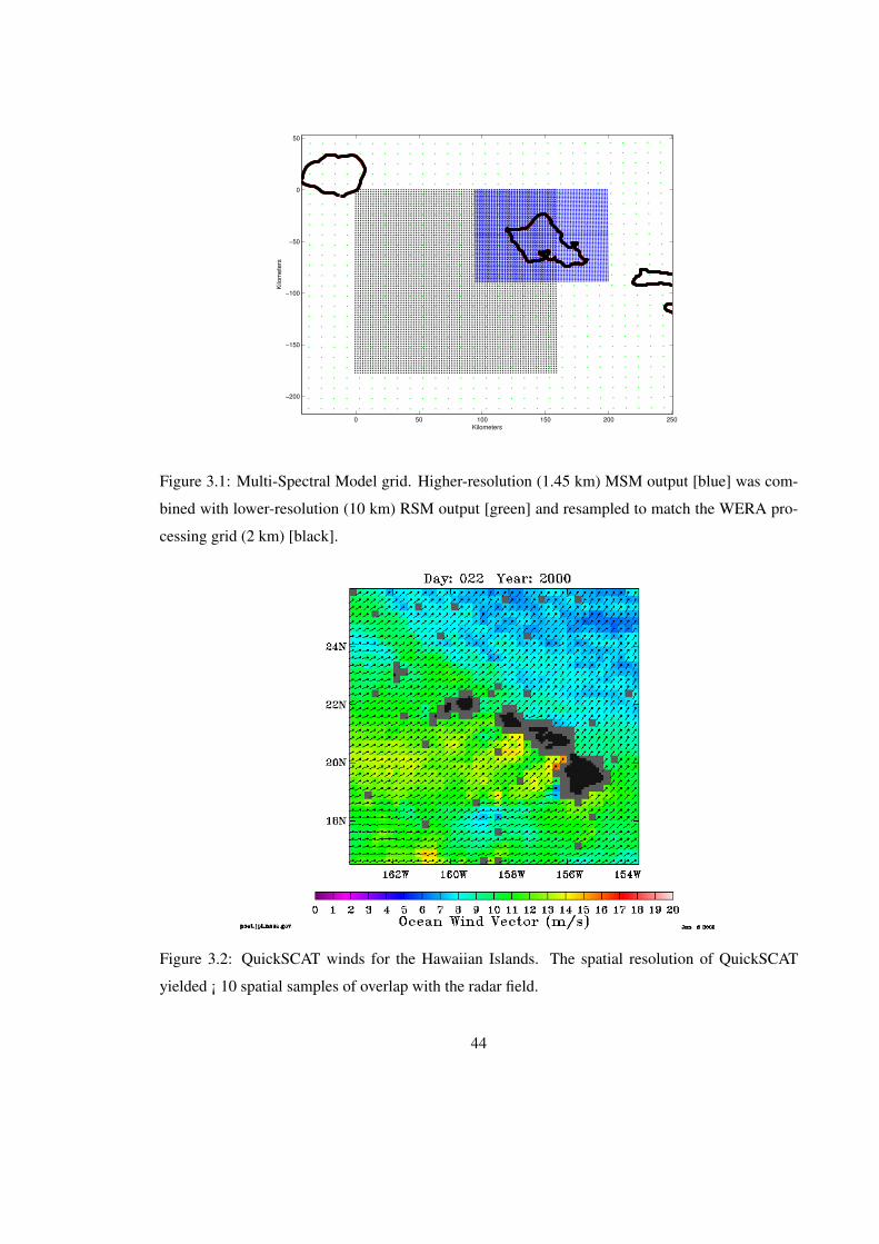
0 50 100 150 200 250
−200
−150
−100
−50
0
50
Kilometers
Kilo
mete
rs
Figure 3.1: Multi-Spectral Model grid. Higher-resolution (1.45 km) MSM output [blue] was com-
bined with lower-resolution (10 km) RSM output [green] and resampled to match the WERA pro-
cessing grid (2 km) [black].
Figure 3.2: QuickSCAT winds for the Hawaiian Islands. The spatial resolution of QuickSCAT
yielded ¡ 10 spatial samples of overlap with the radar field.
44

Figure 3.3: An example radar-derived wind field. Arrows represent wind direction only, no magni-
tude is inferred.
80 90 100 110 120 130 140−110
−100
−90
−80
−70
−60
−50
−40
−30
kilometers
kilo
me
ters
MSM,RSM combined dataset
80 90 100 110 120 130 140−110
−100
−90
−80
−70
−60
−50
−40
−30
kilometers
kilo
me
ters
WERA wind directions
Figure 3.4: Radar wind field compared to MSM output
45
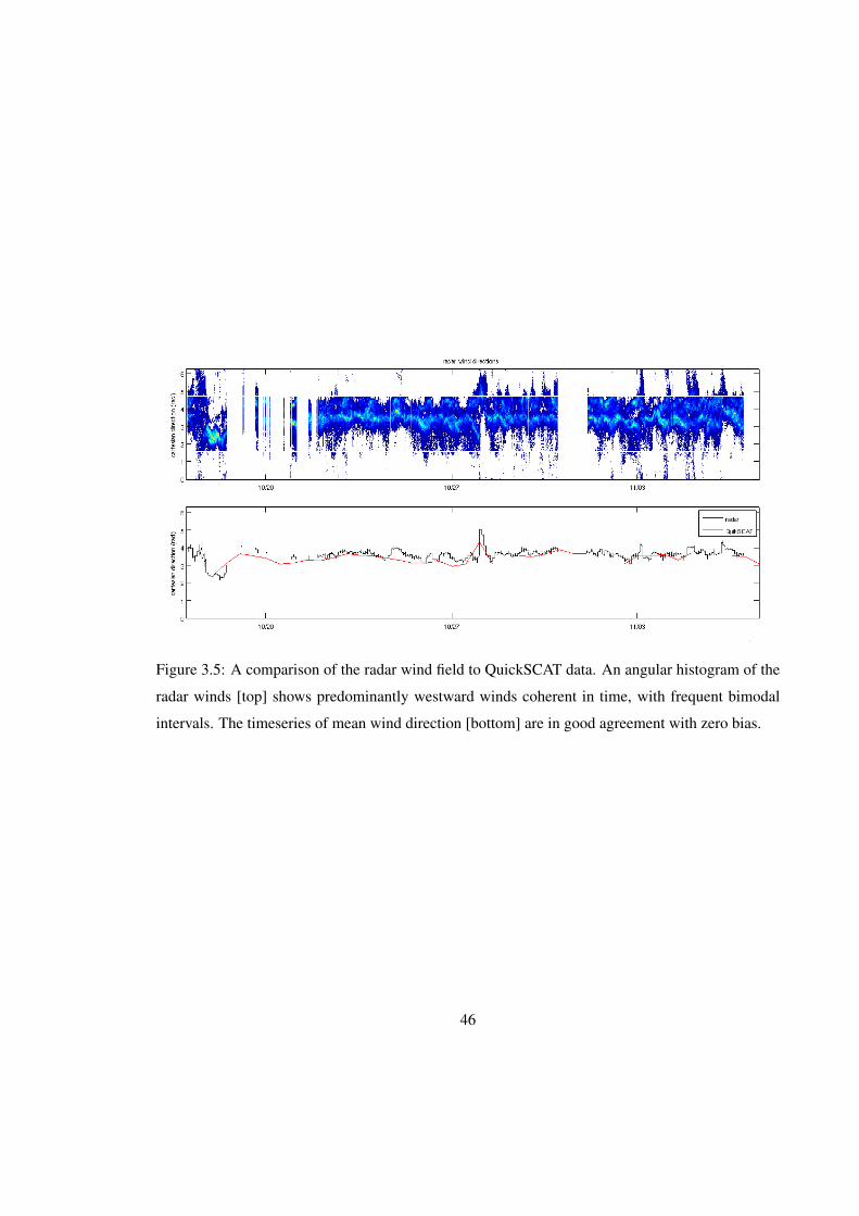
Figure 3.5: A comparison of the radar wind field to QuickSCAT data. An angular histogram of the
radar winds [top] shows predominantly westward winds coherent in time, with frequent bimodal
intervals. The timeseries of mean wind direction [bottom] are in good agreement with zero bias.
46
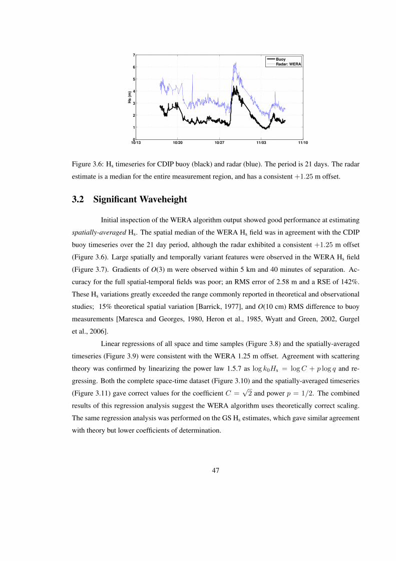
10/13 10/20 10/27 11/03 11/100
1
2
3
4
5
6
7
Hs
(m
)
Buoy
Radar: WERA
Figure 3.6: Hs timeseries for CDIP buoy (black) and radar (blue). The period is 21 days. The radar
estimate is a median for the entire measurement region, and has a consistent +1.25 m offset.
3.2 Significant Waveheight
Initial inspection of the WERA algorithm output showed good performance at estimating
spatially-averaged Hs. The spatial median of the WERA Hs field was in agreement with the CDIP
buoy timeseries over the 21 day period, although the radar exhibited a consistent +1.25 m offset
(Figure 3.6). Large spatially and temporally variant features were observed in the WERA Hs field
(Figure 3.7). Gradients of O(3) m were observed within 5 km and 40 minutes of separation. Ac-
curacy for the full spatial-temporal fields was poor; an RMS error of 2.58 m and a RSE of 142%.
These Hs variations greatly exceeded the range commonly reported in theoretical and observational
studies; 15% theoretical spatial variation [Barrick, 1977], and O(10 cm) RMS difference to buoy
measurements [Maresca and Georges, 1980, Heron et al., 1985, Wyatt and Green, 2002, Gurgel
et al., 2006].
Linear regressions of all space and time samples (Figure 3.8) and the spatially-averaged
timeseries (Figure 3.9) were consistent with the WERA 1.25 m offset. Agreement with scattering
theory was confirmed by linearizing the power law 1.5.7 as log k0Hs = logC + p log q and re-
gressing. Both the complete space-time dataset (Figure 3.10) and the spatially-averaged timeseries
(Figure 3.11) gave correct values for the coefficient C =√
2 and power p = 1/2. The combined
results of this regression analysis suggest the WERA algorithm uses theoretically correct scaling.
The same regression analysis was performed on the GS Hs estimates, which gave similar agreement
with theory but lower coefficients of determination.
47
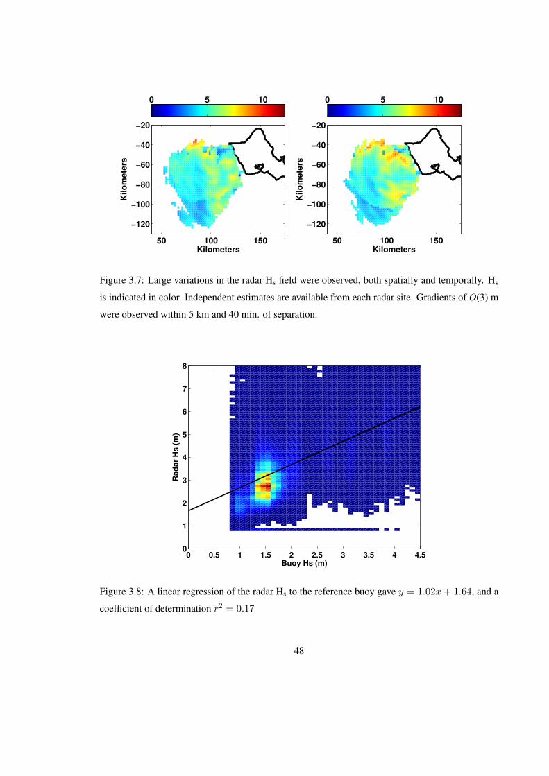
50 100 150
−120
−100
−80
−60
−40
−20
Kilometers
Kilometers
0 5 10
50 100 150
−120
−100
−80
−60
−40
−20
Kilometers
Kilometers
0 5 10
Figure 3.7: Large variations in the radar Hs field were observed, both spatially and temporally. Hs
is indicated in color. Independent estimates are available from each radar site. Gradients of O(3) m
were observed within 5 km and 40 min. of separation.
0 0.5 1 1.5 2 2.5 3 3.5 4 4.50
1
2
3
4
5
6
7
8
Buoy Hs (m)
Rad
ar
Hs (
m)
Figure 3.8: A linear regression of the radar Hs to the reference buoy gave y = 1.02x+ 1.64, and a
coefficient of determination r2 = 0.17
48
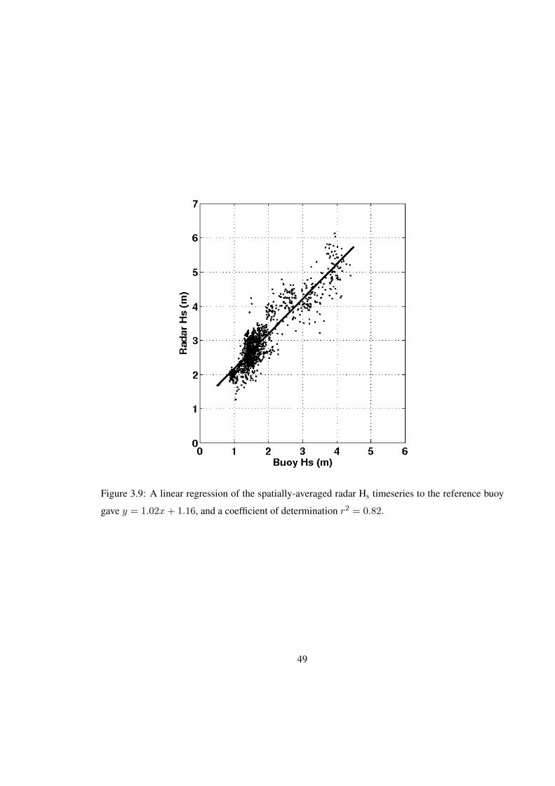
Figure 3.9: A linear regression of the spatially-averaged radar Hs timeseries to the reference buoy
gave y = 1.02x+ 1.16, and a coefficient of determination r2 = 0.82.
49
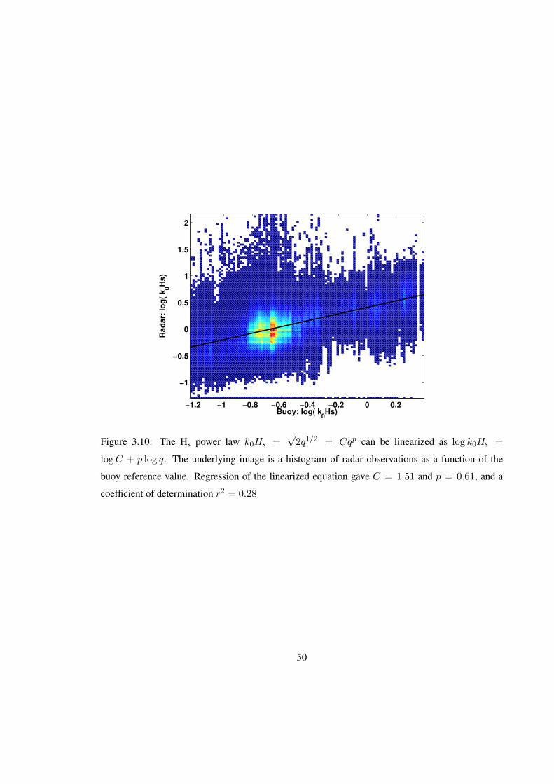
−1.2 −1 −0.8 −0.6 −0.4 −0.2 0 0.2
−1
−0.5
0
0.5
1
1.5
2
Buoy: log( k0Hs)
Rad
ar:
lo
g(
k0H
s)
Figure 3.10: The Hs power law k0Hs =√
2q1/2 = Cqp can be linearized as log k0Hs =
logC + p log q. The underlying image is a histogram of radar observations as a function of the
buoy reference value. Regression of the linearized equation gave C = 1.51 and p = 0.61, and a
coefficient of determination r2 = 0.28
50

−1.4 −1.2 −1 −0.8 −0.6 −0.4 −0.2 0 0.2−1
−0.8
−0.6
−0.4
−0.2
0
0.2
0.4
0.6
0.8
Buoy: log( k0Hs)
Rad
ar:
lo
g(
k0H
s)
Figure 3.11: The same linearized power law regression was calculated for the spatially-averaged
timeseries, yielding C = 1.42 and p = 0.67, and a coefficient of determination r2 = 0.79
Improved Hs accuracy was achieved following the averaging recommendations of Barrick
[1980], as summarized in §1.5.3. Spatially-averaged timeseries were calculated using the median,
arithmetic mean 〈qp〉, inverse quotient 〈q−1〉−p, and inverse quotient to the pth 〈q−p〉−1. Three error
metrics; the rms error, relative standard error, and error bias were calculated for these averaging
methods (Table 3.1). All averaging methods gave improved accuracy compared to the full space-
time data set. The inverse quotient resulted in the highest accuracy for all error metrics. Barrick
[1980] found the inverse quotient to the pth to be the most accurate, with the inverse quotient a close
second. The WERA estimates were moderately improved by spatial averaging, whereas the GS
estimates drastically improved and exceeded the WERA algorithm in accuracy. The most accurate
results were for the GS algorithm using inverse quotient averaging, yielding a rms error of 0.68 m,
RSE error of 38%, and a bias of 1.01.
The improvement in Hs accuracy from spatial averaging is better understood in terms of
the probability distribution. Histograms estimates of the probability distribution were calculated for
the reference buoy and both Hs algorithms. For the full data set, both algorithms had distributions
biased +1-2 m higher than the reference buoy. The inverse quotient mean used in the spatial averag-
ing is heavily weighted towards the lower Hs values, as exhibited by the GS estimates approaching
51

Table 3.1: Hs error analysis
all data median 〈qp〉 〈q−1〉−p 〈q−p〉−1
WERARMS 2.58 1.46 1.74 1.25 1.38RSE 142% 80% 96% 68% 76%bias 2.16 1.87 2.01 1.73 1.82
GSRMS 9.83 2.59 4.94 0.68 1.10RSE 540% 142% 271% 38% 60%bias 3.53 1.96 3.16 1.01 1.51
spatial averages
0 2 4 6 80
0.5
1
1.5
Hs (m)
P(x
)
CDIP Buoy
WERA
GS
0 2 4 6 80
0.5
1
1.5
Hs (m)
P(x
)
CDIP Buoy
WERA
GS
Figure 3.12: Probability distributions were calculated from histograms of the Hs estimates. The
reference buoy distribution [black] is compared to the WERA [blue] and GS [green] algorithm
estimates. Both the full space-time data set [left], and the spatially-averaged [right] distributions
are shown. The effect of the inverse quotient averaging is seen as a weighting of the distributions
towards lower values. Such averaging greatly improves the GS estimate accuracy. The WERA
distribution lacks the necessary lower Hs values.
the reference buoy distribution (Figure 3.12). The WERA distribution lacks lower Hs values and
is less affected from averaging. Thus the large improvement in GS accuracy is due to the inverse
quotient mean shifting the values towards the correct distribution. The WERA estimates benefit
less from averaging because the distribution lacks the lower Hs values. The cutoff in the WERA
distribution below Hs 1 ms−1 is due to a forced minimum in the algorithm. Thus the probability of
the lowest Hs bin is biased. Furthermore, the WERA algorithm applies an empirical weighting to
the spectral energies used in the Hs equation 1.5.5, which may ultimately explain the difference in
accuracy and distribution compared to the un-weighted GS algorithm (see §B).
52
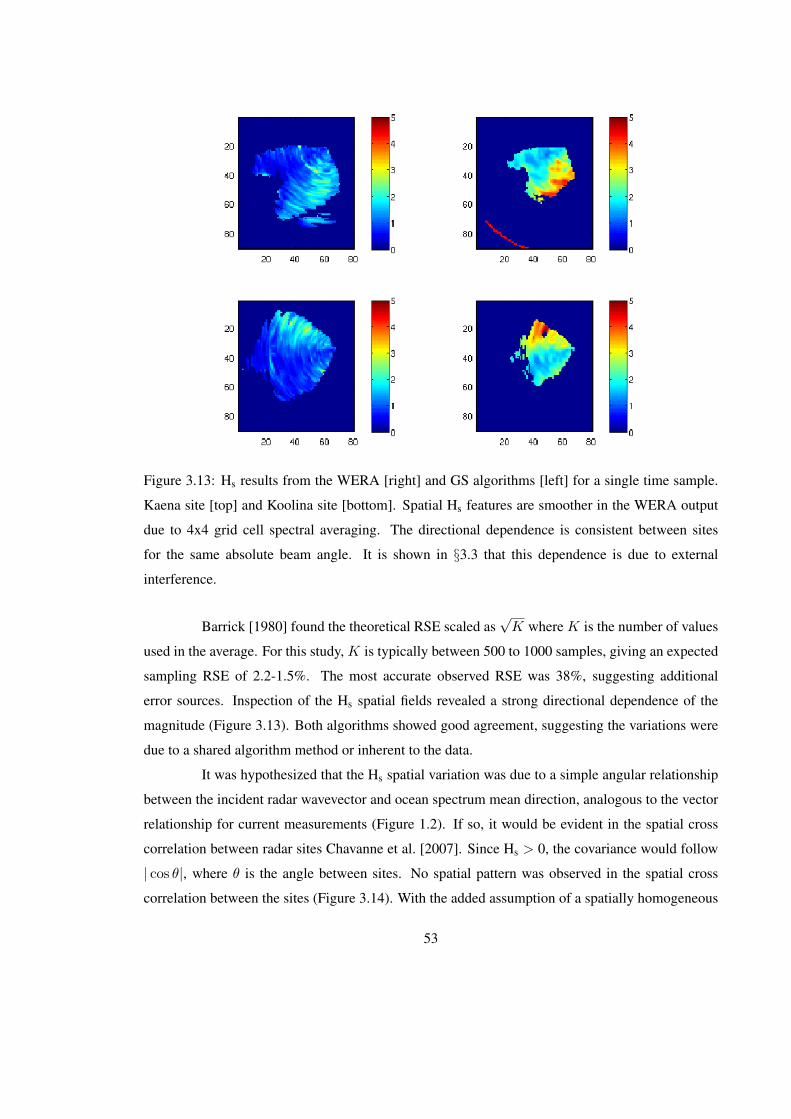
Figure 3.13: Hs results from the WERA [right] and GS algorithms [left] for a single time sample.
Kaena site [top] and Koolina site [bottom]. Spatial Hs features are smoother in the WERA output
due to 4x4 grid cell spectral averaging. The directional dependence is consistent between sites
for the same absolute beam angle. It is shown in §3.3 that this dependence is due to external
interference.
Barrick [1980] found the theoretical RSE scaled as√K where K is the number of values
used in the average. For this study, K is typically between 500 to 1000 samples, giving an expected
sampling RSE of 2.2-1.5%. The most accurate observed RSE was 38%, suggesting additional
error sources. Inspection of the Hs spatial fields revealed a strong directional dependence of the
magnitude (Figure 3.13). Both algorithms showed good agreement, suggesting the variations were
due to a shared algorithm method or inherent to the data.
It was hypothesized that the Hs spatial variation was due to a simple angular relationship
between the incident radar wavevector and ocean spectrum mean direction, analogous to the vector
relationship for current measurements (Figure 1.2). If so, it would be evident in the spatial cross
correlation between radar sites Chavanne et al. [2007]. Since Hs > 0, the covariance would follow
| cos θ|, where θ is the angle between sites. No spatial pattern was observed in the spatial cross
correlation between the sites (Figure 3.14). With the added assumption of a spatially homogeneous
53
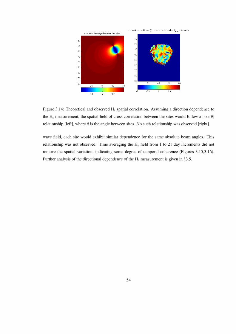
Figure 3.14: Theoretical and observed Hs spatial correlation. Assuming a direction dependence to
the Hs measurement, the spatial field of cross correlation between the sites would follow a | cos θ|relationship [left], where θ is the angle between sites. No such relationship was observed [right].
wave field, each site would exhibit similar dependence for the same absolute beam angles. This
relationship was not observed. Time averaging the Hs field from 1 to 21 day increments did not
remove the spatial variation, indicating some degree of temporal coherence (Figures 3.15,3.16).
Further analysis of the directional dependence of the Hs measurement is given in §3.5.
54

Figure 3.15: The spatial Hs variation is coherent over a 1 day mean.
Figure 3.16: The 21 day median of the Hs field shows the spatial variation is coherent in time. The
combined field [right] can be closely approximated with a site-average (Koolina [left] and Kaena
[center]), although the WERA algorithm uses a more complicated method §B.
55

3.3 Noise Error
3.3.1 Introduction
It was hypothesized that the observed Hs variation could be attributed to noise sources in
the radar measurement. There are two major categories of noise error in radar sampling. Defined
by their effect, they are additive and multiplicative. Multiplicative noise is a consequence of radar
operation, wherein gain factors are introduced, e.g. due to signal attenuation with range and variable
channel strengths. Multiplicative noise is relatively easy to compensate for in processing, and is not
discussed herein. Additive noise results from multiple real signals, e.g. the desired ocean scatter,
external interference, ship echoes, and internal systematic noise. Internal system noise can be caused
by aliased harmonics from the power supply and surrounding electronics, mechanical vibration, and
from thermal noise in the conductors. Generated by the thermal excitation of electrons inside a
conductor, thermal noise is approximately white with a very nearly Gaussian distribution [Nyquist,
1928]. The background, or minimal, variation of the Doppler spectra is electromagnetic and thermal
[Gurgel et al., 2006].
External interference behaves additively [Ponsford et al., 2003] and is range-independent
[Gurgel et al., 2006]. In the HF frequency band, the primary source of interference is anthropogenic
transmissions, and thus commonly referred to as radio frequency interference (RFI). The dominat-
ing source of interference in the HF band is RFI [Molnar et al., 1990]. Due to the ionospheric
propagation and reflection of HF EM waves, unoccupied frequencies of sufficient bandwidth (50-
100 kHz) can be extremely difficult to find. Ionospheric conditions change with solar insolation, are
more suited for reflecting interference sources at night [Ponsford et al., 2003], and can propagate
signals over 1000’s of kilometers.
Canceling additive noise is most difficult when its frequency matches the desired signal.
From the Harmonic Addition Theorem, any linear combination of sine waves with equal frequency
results in a sine wave with the same frequency, but modified amplitude and phase. Given two
sinusoidal functions with the same frequency ω:
ψ1 = A1 sin(ωt+ δ1) (3.3.1)
ψ2 = A2 sin(ωt+ δ2) (3.3.2)
their sum ψ can be expressed as a sinusoidal function with frequency ω:
ψ ≡ ψ1 + ψ2 ≡ A sin(ωt+ δ) (3.3.3)
56
where A and δ are defined as:
A2 = A21 +A2
2 + 2A1A2 cos(δ1 − δ2) (3.3.4)
tan(δ) =A1 sin δ1 +A2 sin δ2
A1 cos δ1 +A2 cos δ2(3.3.5)
From Equation 3.3.4, the amplitude of the total sinusoid ψ does not behave additively. It
depends on the phase difference δ1 − δ2. This non-additive behavior for the total amplitude A is
the reason why simple techniques, e.g. averaging or subtraction, do not work to remove additive
noise error. Noise at signal frequencies modifies the amplitudes unpredictably as a function of their
phase relationship. The actual signal sinusoid ψ1 can be recovered with knowledge of the total ψ
and noise ψ2 sinusoids.
3.3.2 Observations
Inspection of the raw antenna spectra (Figure 3.17) and beamformed noise levels (Figure
3.21) identified the characteristic noise sources. Thermal background noise was observed in sam-
ples with the highest SNR; up to 100 dB below the first order Bragg peaks (Figure 3.17). Samples
with low SNR were contaminated with ringing, full-spectrum noise exhibiting range-independence.
Broad spectral peaks at various ranges were due to 60 Hz harmonics of the power supply, and possi-
bly other unknown sources (Figure 3.17). Observations by Gurgel et al. [2006] have shown similar
noise characteristics (Figures 3.18). Beamforming (§C) and noise level estimation (§3.3.3) were
used to investigate the spatial characteristics of noise sources (Figure 3.21). The deformation of
Doppler spectra by RFI varied across the sampling field. In the direction of a RFI source, Bragg
peaks were deformed, preventing detection of the S1:S2 null (Figure 3.20), and introduced ampli-
tude noise in the S2 region. Outside of RFI source directions, samples at the same time and range
were usable (Figure 3.19).
Additive noise of sufficient energy prevent accurate estimation of second order energy.
Ideal spectra have sufficiently high SNR that both the first and second order signal are well above
the noise floor (Figure 3.19). Unusable spectra have very low SNR due to the full-spectrum range-
independent noise (Figure 3.20). In terms of accuracy and data quality control, such spectra are
not a problem as they can be unambiguously rejected. Rather, samples with intermediate SNR
pose the greatest difficulty. For intermediate SNR, Bragg peaks are easily identified, albeit with
frequency errors due to noise energy in the centroid amplitude weighting. In contrast, the second
order sidebands are completely contaminated. Noise energy introduces an amplitude ambiguity
57

Figure 3.17: Two example spectra illustrating periods of low [top] and high [bottom] noise are
given for a single channel. The thermal background is observed in the low noise example at 100
dB below the Bragg peaks. Broad spectral peaks at various ranges are due to 60 Hz harmonics and
other systematic noise. The primary noise source is external interference, which is characterized by
range-independence [bottom].
58
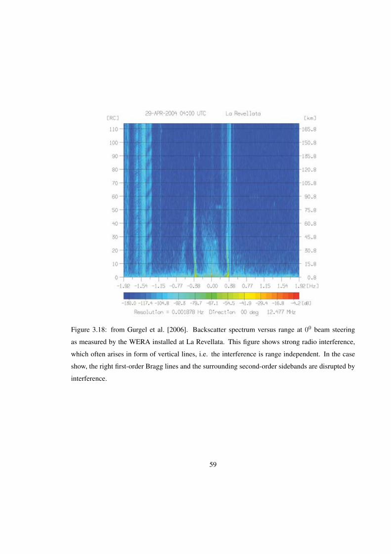
Figure 3.18: from Gurgel et al. [2006]. Backscatter spectrum versus range at 00 beam steering
as measured by the WERA installed at La Revellata. This figure shows strong radio interference,
which often arises in form of vertical lines, i.e. the interference is range independent. In the case
show, the right first-order Bragg lines and the surrounding second-order sidebands are disrupted by
interference.
59

Figure 3.19: An ideal Doppler spectrum [black] showing a clearly defined first order peak and
second order sidebands. The S1 width is defined, and detected by the processing algorithm, by the
nulls on each side. Most of the S2 energy is above the noise level [blue].
60

Figure 3.20: A contaminated Doppler spectrum [black], with deformed first order peak. A lack of
clear nulls separating the S1 and S2 regions prevents accurate estimation of either energy. The S2
region is beneath the noise level [blue].
61

Figure 3.21: Two example noise fields illustrating period of low [bottom] and high [top] noise.
Estimated noise levels are given in color. The primary noise source is external interference, which
is characterized by range-independent beams from specific directions.
62

which cannot be recovered. The result is erroneous Hs estimates due to the inclusion of noise in the
energy integral.
63

3.3.3 Noise Estimation
For estimating the noise level, Heron and Heron [2001] proposed fitting the entire Doppler
spectrum to a statistical distribution for noise. By iteratively discarding signal, i.e. spectral points
with large values, the distribution converged to a model for the noise. This method assumes the
noise is white, and thus the power spectrum of noise is Rayleigh distributed.
The Rayleigh distribution has one parameter, p. The Rayleigh probability density and
cumulative distribution functions are:
f(x; p) =x
p2e−x2
2p2 (3.3.6)
F (x; p) = 1− e−x2
2p2 (3.3.7)
for x ∈ [0,∞) (3.3.8)
The mean and variance of a Rayleigh random variable are:
µ(X) = p
√π
2(3.3.9)
σ = p2 4− π2
(3.3.10)
Given N independent and identically distributed Rayleigh random variables with parameter p, the
maximum likelihood estimate (MLE) of p is:
p =
√√√√ 1
2N
N∑i=1
x2i (3.3.11)
Four methods were evaluated for estimating the mean noise level. The first three were
direct calculations of the spectral power mean, median, and maximum likelihood estimate (MLE).
The fourth method followed Heron and Heron [2001]; a linear least squares regression of the ordered
spectral data to a Rayleigh cumulative distribution function (CDF) (Figure 3.22). All methods used
the same iterative scheme which discarded outliers based on the variance.
The MLE estimate did not converge to the noise distribution due to the x2 weighting in its
equation, which acts to bias it towards greater-valued signal. As a first approximation, the MLE is a
poor fit to the sum of a Rayleigh and signal (unknown) distribution. Likewise, the median estimate
performed better than the mean, as it was not weighted towards extreme signal values. Iterations
64

Figure 3.22: Ordered spectral values [black] compared to various direct methods for estimating the
noise CDF. X-axis is CDF probability. Y-axis is spectral powers. Low-power noise P < 1 · 105
comprises 90% of the CDF. The mean [blue] and median [green] closely approximate the noise
distribution. The MLE [red] is biased towards larger signal values due to the x2 weighting in its
calculation.
65
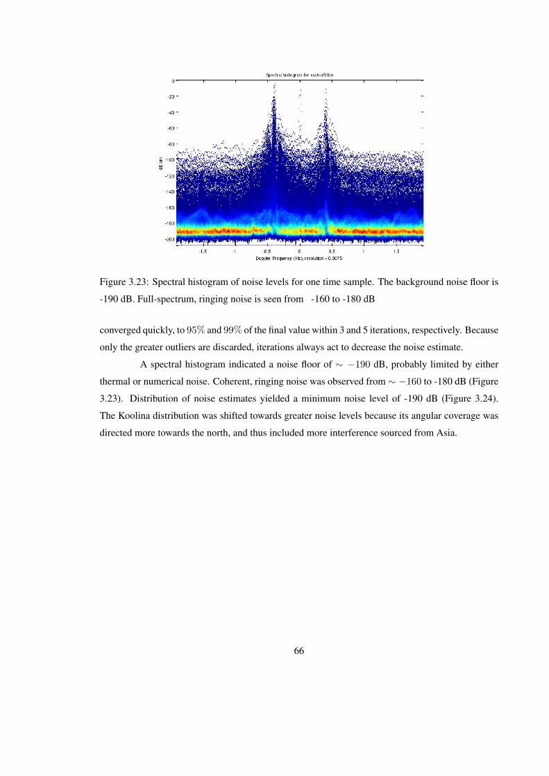
Figure 3.23: Spectral histogram of noise levels for one time sample. The background noise floor is
-190 dB. Full-spectrum, ringing noise is seen from -160 to -180 dB
converged quickly, to 95% and 99% of the final value within 3 and 5 iterations, respectively. Because
only the greater outliers are discarded, iterations always act to decrease the noise estimate.
A spectral histogram indicated a noise floor of ∼ −190 dB, probably limited by either
thermal or numerical noise. Coherent, ringing noise was observed from∼ −160 to -180 dB (Figure
3.23). Distribution of noise estimates yielded a minimum noise level of -190 dB (Figure 3.24).
The Koolina distribution was shifted towards greater noise levels because its angular coverage was
directed more towards the north, and thus included more interference sourced from Asia.
66

Figure 3.24: Noise distributions for Kaena [red] and Koolina [blue]. Background noise level is -190
dB. The Koolina distribution is shifted towards greater noise values because its angular coverage
intercepts Asian RFI sources.
67
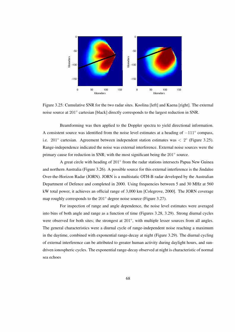
Figure 3.25: Cumulative SNR for the two radar sites. Koolina [left] and Kaena [right]. The external
noise source at 201 cartesian [black] directly corresponds to the largest reduction in SNR.
Beamforming was then applied to the Doppler spectra to yield directional information.
A consistent source was identified from the noise level estimates at a heading of −111 compass,
i.e. 201 cartesian. Agreement between independent station estimates was < 2 (Figure 3.25).
Range-independence indicated the noise was external interference. External noise sources were the
primary cause for reduction in SNR; with the most significant being the 201 source.
A great circle with heading of 201 from the radar stations intersects Papua New Guinea
and northern Australia (Figure 3.26). A possible source for this external interference is the Jindalee
Over-the-Horizon Radar (JORN). JORN is a multistatic OTH-B radar developed by the Australian
Department of Defence and completed in 2000. Using frequencies between 5 and 30 MHz at 560
kW total power, it achieves an official range of 3,000 km [Colegrove, 2000]. The JORN coverage
map roughly corresponds to the 201 degree noise source (Figure 3.27).
For inspection of range and angle dependence, the noise level estimates were averaged
into bins of both angle and range as a function of time (Figures 3.28, 3.29). Strong diurnal cycles
were observed for both sites; the strongest at 201, with multiple lesser sources from all angles.
The general characteristics were a diurnal cycle of range-independent noise reaching a maximum
in the daytime, combined with exponential range-decay at night (Figure 3.29). The diurnal cycling
of external interference can be attributed to greater human activity during daylight hours, and sun-
driven ionospheric cycles. The exponential range-decay observed at night is characteristic of normal
sea echoes
68
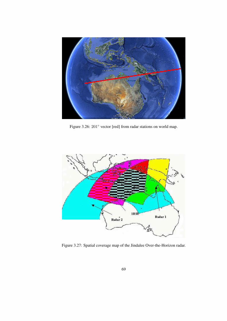
Figure 3.26: 201 vector [red] from radar stations on world map.
Figure 3.27: Spatial coverage map of the Jindalee Over-the-Horizon radar.
69

Figure 3.28: Noise as a function of angle and time. Angles have been averaged into 100 equal width
bins. Time is on the X-axis. The Y-axis is absolute, i.e. world, angle. Thus a heading of West = π
would point at the same point at infinite range for both plots. Koolina [top] and Kaena [bottom].
Both sites exhibit a diurnal noise source at 3.5rad ' 200.
Figure 3.29: Noise as a function of range and time. External interference is seen as range-
independent diurnal cycles. Time periods without external interference show exponential decay
with range characteristic of normal radar echoes.
70
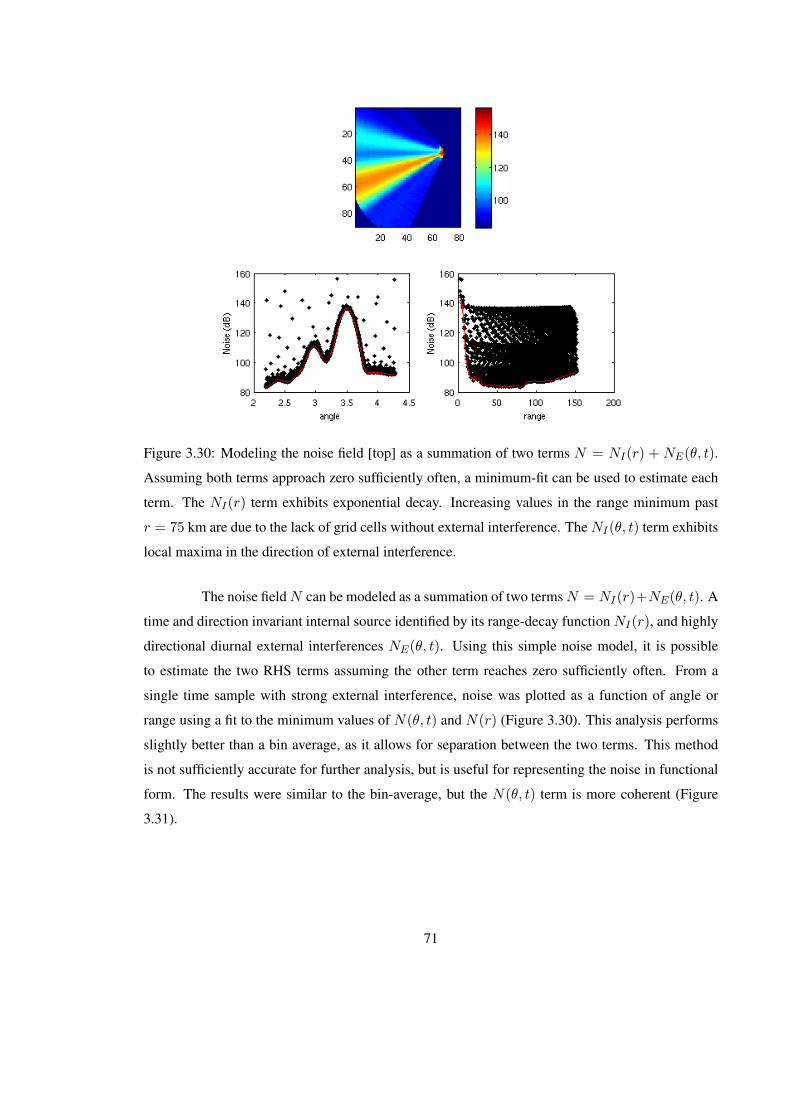
Figure 3.30: Modeling the noise field [top] as a summation of two terms N = NI(r) + NE(θ, t).
Assuming both terms approach zero sufficiently often, a minimum-fit can be used to estimate each
term. The NI(r) term exhibits exponential decay. Increasing values in the range minimum past
r = 75 km are due to the lack of grid cells without external interference. The NI(θ, t) term exhibits
local maxima in the direction of external interference.
The noise fieldN can be modeled as a summation of two termsN = NI(r)+NE(θ, t). A
time and direction invariant internal source identified by its range-decay function NI(r), and highly
directional diurnal external interferences NE(θ, t). Using this simple noise model, it is possible
to estimate the two RHS terms assuming the other term reaches zero sufficiently often. From a
single time sample with strong external interference, noise was plotted as a function of angle or
range using a fit to the minimum values of N(θ, t) and N(r) (Figure 3.30). This analysis performs
slightly better than a bin average, as it allows for separation between the two terms. This method
is not sufficiently accurate for further analysis, but is useful for representing the noise in functional
form. The results were similar to the bin-average, but the N(θ, t) term is more coherent (Figure
3.31).
71

Figure 3.31: Results from the noise model; noise level as a function of angle and time NI(θ, t).
Both radar sites exhibit the 201 noise source, and Koolina has a very strong intermittent noise
source at 125
72
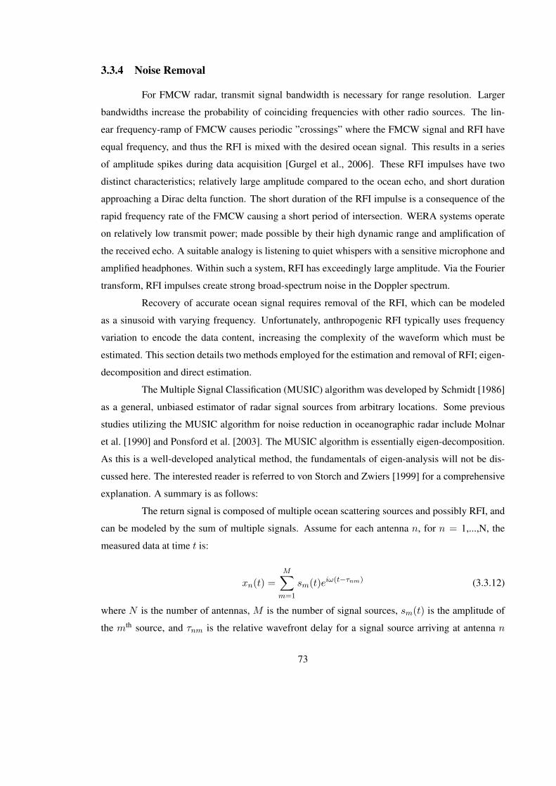
3.3.4 Noise Removal
For FMCW radar, transmit signal bandwidth is necessary for range resolution. Larger
bandwidths increase the probability of coinciding frequencies with other radio sources. The lin-
ear frequency-ramp of FMCW causes periodic ”crossings” where the FMCW signal and RFI have
equal frequency, and thus the RFI is mixed with the desired ocean signal. This results in a series
of amplitude spikes during data acquisition [Gurgel et al., 2006]. These RFI impulses have two
distinct characteristics; relatively large amplitude compared to the ocean echo, and short duration
approaching a Dirac delta function. The short duration of the RFI impulse is a consequence of the
rapid frequency rate of the FMCW causing a short period of intersection. WERA systems operate
on relatively low transmit power; made possible by their high dynamic range and amplification of
the received echo. A suitable analogy is listening to quiet whispers with a sensitive microphone and
amplified headphones. Within such a system, RFI has exceedingly large amplitude. Via the Fourier
transform, RFI impulses create strong broad-spectrum noise in the Doppler spectrum.
Recovery of accurate ocean signal requires removal of the RFI, which can be modeled
as a sinusoid with varying frequency. Unfortunately, anthropogenic RFI typically uses frequency
variation to encode the data content, increasing the complexity of the waveform which must be
estimated. This section details two methods employed for the estimation and removal of RFI; eigen-
decomposition and direct estimation.
The Multiple Signal Classification (MUSIC) algorithm was developed by Schmidt [1986]
as a general, unbiased estimator of radar signal sources from arbitrary locations. Some previous
studies utilizing the MUSIC algorithm for noise reduction in oceanographic radar include Molnar
et al. [1990] and Ponsford et al. [2003]. The MUSIC algorithm is essentially eigen-decomposition.
As this is a well-developed analytical method, the fundamentals of eigen-analysis will not be dis-
cussed here. The interested reader is referred to von Storch and Zwiers [1999] for a comprehensive
explanation. A summary is as follows:
The return signal is composed of multiple ocean scattering sources and possibly RFI, and
can be modeled by the sum of multiple signals. Assume for each antenna n, for n = 1,...,N, the
measured data at time t is:
xn(t) =
M∑m=1
sm(t)eiω(t−τnm) (3.3.12)
where N is the number of antennas, M is the number of signal sources, sm(t) is the amplitude of
the mth source, and τnm is the relative wavefront delay for a signal source arriving at antenna n
73

as a function of direction. In matrix notation, equation 3.3.12 can be written as X = AS. The
covariance matrix of the measurements can then be expressed as:
Rxx = ASAH (3.3.13)
where A is an N ×M direction matrix, with the column vector am associated with the direction of
the mth signal. A can also be understood as a beamforming array factor, as in equation C.0.33.
From spectral estimation theory, it is known that the N eigenvectors of Rxx can be par-
titioned into two subsets, spanning a signal and noise subspace, with respective eigenspace indices
m <= d,m > d. Assuming that RFI corresponds to the largest eigenvalues, the threshold index d
is chosen. The RFI-free signal can then be constructed as:
Xr = X −d∑
m=1
eHmXemeHmem
(3.3.14)
Thus MUSIC is straightforward eigen-decomposition of the received signals, with the
additional step of calculating beamformed spectra as a function of direction. The covariance matrix
is calculated as antenna covariance. The threshold d can be data-adaptive or predetermined, with
the goal of separating RFI from the uncorrelated ocean scatter.
The MUSIC algorithm was applied to a time period of strong RFI noise. The resulting
eigenvalues had uniform difference, with no clear indication of noise vs. signal subspaces. The
greatest eigenvalue was chosen to estimate the noise eigenspace. The resulting spectrum Xr had no
significant reduction in noise (Figure 3.32).
A similar alternative to the MUSIC algorithm is an eigen-decomposition of the range
covariance matrix [Jun et al., 2004]. Since RFI is known to have temporal range coherence, it is
reasonable to expect this variation could be limited to a distinct subspace.
For this analysis, the same data sample was beamsteered directly at the RFI source using
a linear array factor (Figure 3.33). Strong, range-independent eigenfunctions were found, indicative
of RFI noise (Figure 3.34). The ocean signal energy did not map to a separate eigenspace, but
rather overlapped the same eigenmodes as the RFI. To clarify, the form of the RFI eigenmodes
was resolved by high-pass filtering the spectrum to include only the higher noise frequencies, i.e.
remove all ocean signal (Figure 3.35). Attempts at filtering the spectra using only the stronger,
range-independent noise eigenmodes were unsuccessful at removing the RFI.
An alternative effort was made to subtract the RFI via direct estimation of its amplitude
and phase. The amplitude was estimated independently for each frequency as the mean energy for
74
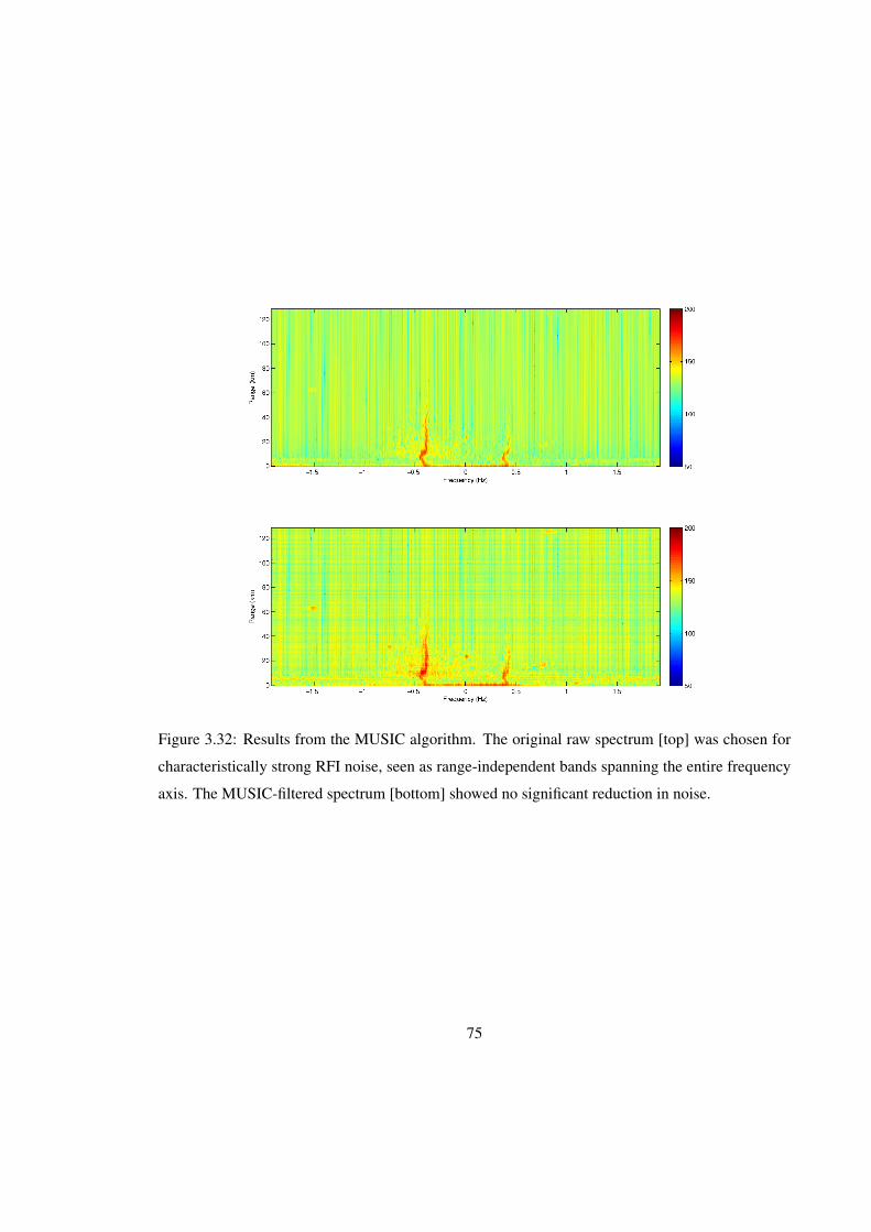
Figure 3.32: Results from the MUSIC algorithm. The original raw spectrum [top] was chosen for
characteristically strong RFI noise, seen as range-independent bands spanning the entire frequency
axis. The MUSIC-filtered spectrum [bottom] showed no significant reduction in noise.
75
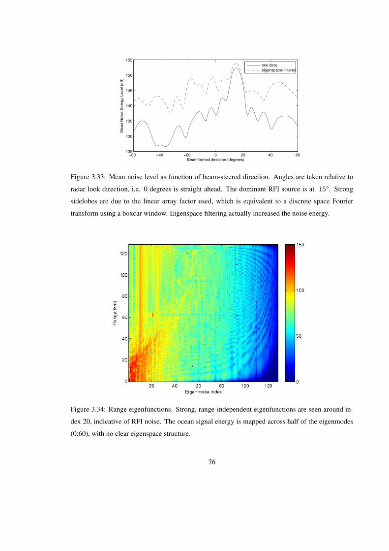
−60 −40 −20 0 20 40 60125
130
135
140
145
150
155
Beamformed direction (degrees)
Me
an
No
ise
En
erg
y L
eve
l (d
B)
raw data
eigenspace−filtered
Figure 3.33: Mean noise level as function of beam-steered direction. Angles are taken relative to
radar look direction, i.e. 0 degrees is straight ahead. The dominant RFI source is at 15. Strong
sidelobes are due to the linear array factor used, which is equivalent to a discrete space Fourier
transform using a boxcar window. Eigenspace filtering actually increased the noise energy.
Figure 3.34: Range eigenfunctions. Strong, range-independent eigenfunctions are seen around in-
dex 20, indicative of RFI noise. The ocean signal energy is mapped across half of the eigenmodes
(0:60), with no clear eigenspace structure.
76
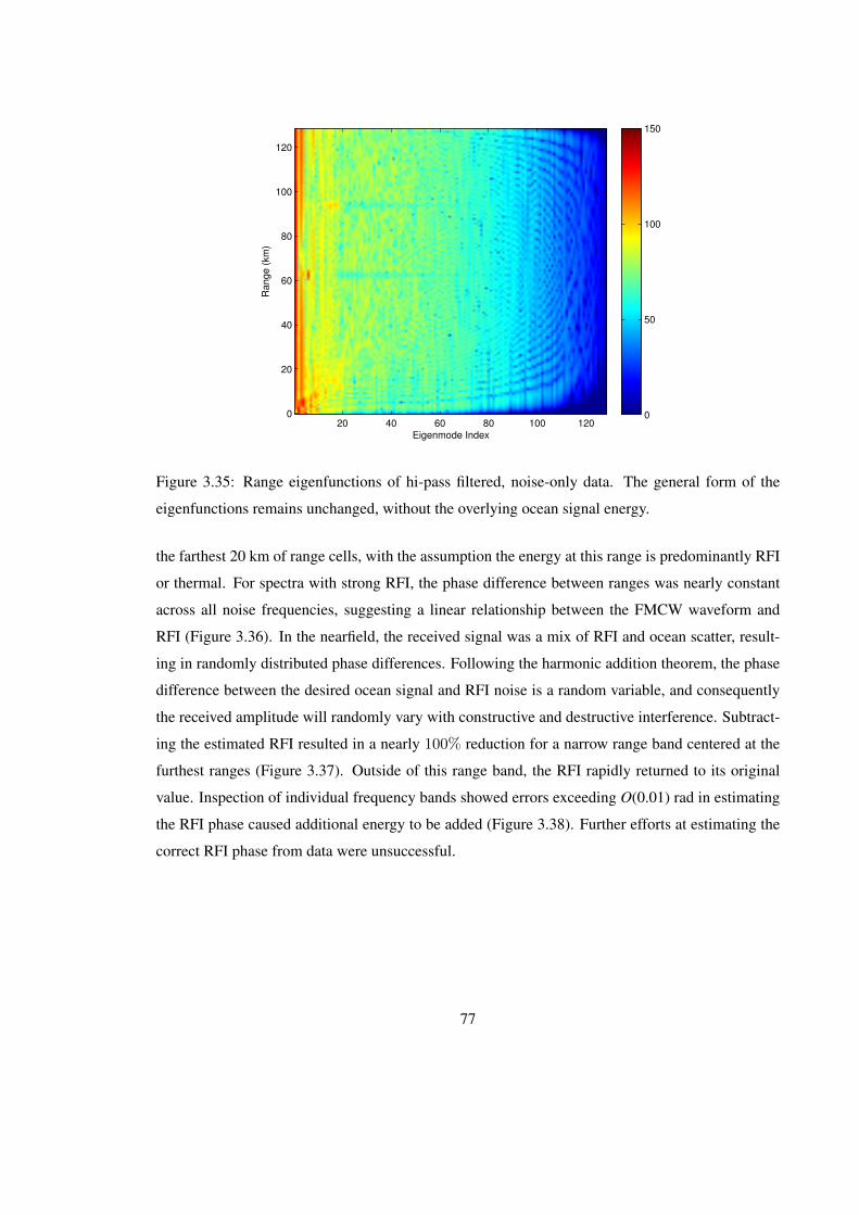
Eigenmode Index
Range (
km
)
20 40 60 80 100 1200
20
40
60
80
100
120
0
50
100
150
Figure 3.35: Range eigenfunctions of hi-pass filtered, noise-only data. The general form of the
eigenfunctions remains unchanged, without the overlying ocean signal energy.
the farthest 20 km of range cells, with the assumption the energy at this range is predominantly RFI
or thermal. For spectra with strong RFI, the phase difference between ranges was nearly constant
across all noise frequencies, suggesting a linear relationship between the FMCW waveform and
RFI (Figure 3.36). In the nearfield, the received signal was a mix of RFI and ocean scatter, result-
ing in randomly distributed phase differences. Following the harmonic addition theorem, the phase
difference between the desired ocean signal and RFI noise is a random variable, and consequently
the received amplitude will randomly vary with constructive and destructive interference. Subtract-
ing the estimated RFI resulted in a nearly 100% reduction for a narrow range band centered at the
furthest ranges (Figure 3.37). Outside of this range band, the RFI rapidly returned to its original
value. Inspection of individual frequency bands showed errors exceeding O(0.01) rad in estimating
the RFI phase caused additional energy to be added (Figure 3.38). Further efforts at estimating the
correct RFI phase from data were unsuccessful.
77
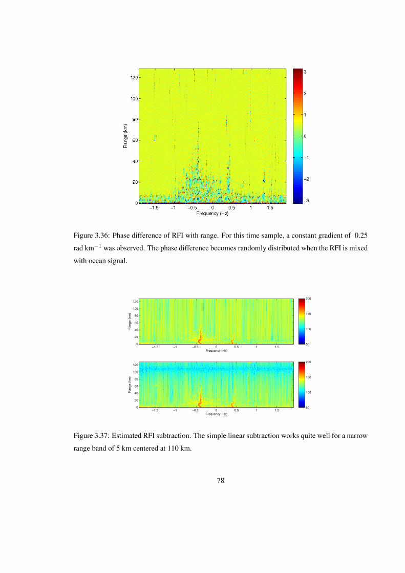
Figure 3.36: Phase difference of RFI with range. For this time sample, a constant gradient of 0.25
rad km−1 was observed. The phase difference becomes randomly distributed when the RFI is mixed
with ocean signal.
Frequency (Hz)
Range (
km
)
−1.5 −1 −0.5 0 0.5 1 1.50
20
40
60
80
100
120
Frequency (Hz)
Range (
km
)
−1.5 −1 −0.5 0 0.5 1 1.50
20
40
60
80
100
120
50
100
150
200
50
100
150
200
Figure 3.37: Estimated RFI subtraction. The simple linear subtraction works quite well for a narrow
range band of 5 km centered at 110 km.
78

Figure 3.38: The effect of subtracting RFI noise with an incorrect phase estimate. A single fre-
quency band is shown, chosen outside the frequency range of ocean scattering. Thus the raw data
represents entirely RFI noise. At 110 km, the RFI phase estimate is accurate, and the amplitude is
reduced ∼ 30 dB. At 60 km, the phase estimate is π/2 radians out of phase, and no cancellation
occurs. By 20 km, the phase estimate is π radians out of phase, and energy is added to the spectrum.
79

3.4 Significant Waveheight Regression Analysis
To further inspect the effects of RFI on radar-derived Hs estimates, linear regression anal-
ysis was performed on the Hs estimates from both algorithms. The 21 day study period, with N =
1222 temporal samples were linearly regressed to the CDIP buoy timeseries. Outside the directions
of external interference, correlation coefficients were highest; 0.6 and 0.9 for the GS and WERA
algorithms, respectively. Spatial regions with the highest correlation had slope and offset of 1,0
(Figures 3.39, 3.40). Combining estimates from both sites improved overall accuracy, but reduced
peak accuracy; i.e. maximum correlation and RMS error, and introduced spatial discontinuities.
Poor accuracy occurred near 200 cartesian, i.e. the direction of the dominant RFI source.
The same regression analysis was repeated after removing time samples with noise lev-
els N > 50 dB, in an angular region centered at 200. The entire spatial field was removed for
these time samples to prevent spatial bias in the correlation. Regression results were significantly
improved in the region 200, yielding increased coefficients of determination and decreased RMS
error (Figure 3.40, 3.41).
80

Figure 3.39: Hs linear regression coefficients. WERA [top] and GS algorithm [bottom]. Koolina
[left], Kaena [center], site-combined [right]. Units for the offset are meters.
81
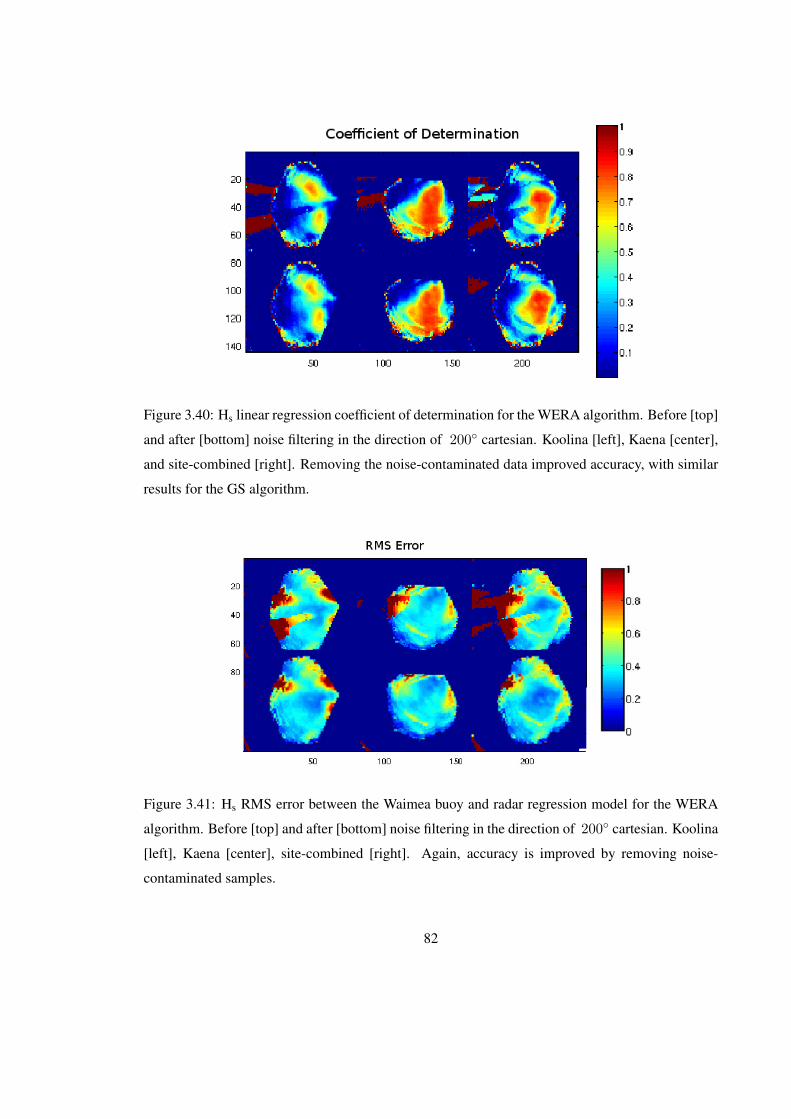
Figure 3.40: Hs linear regression coefficient of determination for the WERA algorithm. Before [top]
and after [bottom] noise filtering in the direction of 200 cartesian. Koolina [left], Kaena [center],
and site-combined [right]. Removing the noise-contaminated data improved accuracy, with similar
results for the GS algorithm.
Figure 3.41: Hs RMS error between the Waimea buoy and radar regression model for the WERA
algorithm. Before [top] and after [bottom] noise filtering in the direction of 200 cartesian. Koolina
[left], Kaena [center], site-combined [right]. Again, accuracy is improved by removing noise-
contaminated samples.
82

3.5 Electromagnetic Scattering: Second Order Integral
Weber and Barrick [1977] identified conditions in which the dominant wave direction
is perpendicular to the radar beam as being error prone for the Hs equation 1.5.5. Barrick [1977]
concluded the Hs equation was weakly dependent on the radar-wave direction. Maresca and Georges
[1980] noted failure of the Hs equation on highly directional synthetic spectra, due to the increased
sensitivity of the S2 energy to direction. As discussed in the proceeding section, the Hs spatial
variation could not be fully explained in terms of a signal-to-noise relationship. Thus an analysis of
the second order integral relation was motivated.
As derived by Derr [1972], the second order integral relation, hereafter S2 integral, is:
σvv(ωD) = 16πk40
∑±
∫ ∞−∞
∫ ∞−∞
dk|ΓT (±k1,±k2)|2W (±k1)W (±k2)δ(ωD±ω1±ω2) (3.5.1)
where σvv(ωD) is the second order Doppler energy, k1,k2 are the interacting first order ocean
wavevectors, W (k) is the directional spatial waveheight spectrum of the ocean, and ΓT is the com-
bined electromagnetic and hydrodynamic coupling coefficient, hereafter coupling coefficient.
The first fundamental theoretical constraint for second order scattering is the Bragg reso-
nance condition k1 +k2 = kB , where kB is the Bragg wavevector. For this discussion and dataset,
a backscattering configuration was used, and thus the Bragg wavevector is exactly twice the radar
wavevector; kB = 2kr. The second constraint is expressed in the S2 integral as δ(ωD ± ω1 ± ω2).
That is, the observed Doppler frequency ωD for a given pair of ocean wavevectors is determined by
their frequency sum. To clarify, the integral is over all ocean wavevector space, allowing for all pos-
sible second order combinations. The two W (k) terms are restricted to the Bragg resonance vector
relation. Similarly for the coupling coefficient. The Doppler frequency ωD at which each second
order wavevector combination will be observed, is determined by their frequency sum ωD±ω1±ω2.
Additional complexity is added by the summation term∑±, which is a consequence of deriving
the S2 integral as an average.
For numerical evaluation and visualization, it is easiest to express the ocean wavevectors
as symmetrical about the integration wavevector k1 = 1/2kr + k, k2 = 1/2kr − k.
The two aforementioned constraints on second order scattering define four independent
Doppler frequency surfaces in wavevector space (Figure 3.42). The ωD+ω1 +ω2 and ωD−ω1−ω2,
hereafter summation frequencies, only contribute to Doppler frequencies |ωD| > fB . Conversely,
the the ωD+ω1−ω2 and ωD−ω1 +ω2, hereafter difference frequencies, only contribute to Doppler
83
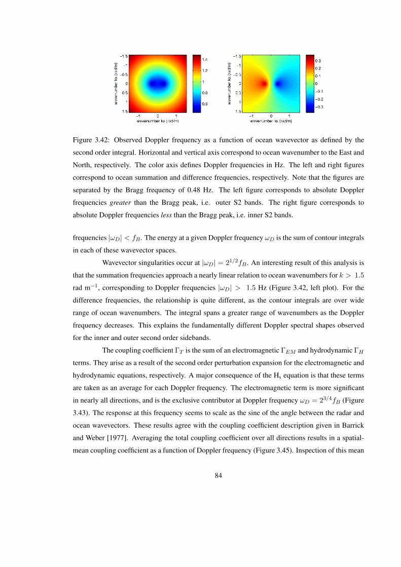
Figure 3.42: Observed Doppler frequency as a function of ocean wavevector as defined by the
second order integral. Horizontal and vertical axis correspond to ocean wavenumber to the East and
North, respectively. The color axis defines Doppler frequencies in Hz. The left and right figures
correspond to ocean summation and difference frequencies, respectively. Note that the figures are
separated by the Bragg frequency of 0.48 Hz. The left figure corresponds to absolute Doppler
frequencies greater than the Bragg peak, i.e. outer S2 bands. The right figure corresponds to
absolute Doppler frequencies less than the Bragg peak, i.e. inner S2 bands.
frequencies |ωD| < fB . The energy at a given Doppler frequency ωD is the sum of contour integrals
in each of these wavevector spaces.
Wavevector singularities occur at |ωD| = 21/2fB . An interesting result of this analysis is
that the summation frequencies approach a nearly linear relation to ocean wavenumbers for k > 1.5
rad m−1, corresponding to Doppler frequencies |ωD| > 1.5 Hz (Figure 3.42, left plot). For the
difference frequencies, the relationship is quite different, as the contour integrals are over wide
range of ocean wavenumbers. The integral spans a greater range of wavenumbers as the Doppler
frequency decreases. This explains the fundamentally different Doppler spectral shapes observed
for the inner and outer second order sidebands.
The coupling coefficient ΓT is the sum of an electromagnetic ΓEM and hydrodynamic ΓH
terms. They arise as a result of the second order perturbation expansion for the electromagnetic and
hydrodynamic equations, respectively. A major consequence of the Hs equation is that these terms
are taken as an average for each Doppler frequency. The electromagnetic term is more significant
in nearly all directions, and is the exclusive contributor at Doppler frequency ωD = 23/4fB (Figure
3.43). The response at this frequency seems to scale as the sine of the angle between the radar and
ocean wavevectors. These results agree with the coupling coefficient description given in Barrick
and Weber [1977]. Averaging the total coupling coefficient over all directions results in a spatial-
mean coupling coefficient as a function of Doppler frequency (Figure 3.45). Inspection of this mean
84

Ocean wavenumber kx (rad/m)
Ocean w
avenum
ber
ky (
rad/m
)
−1 0 1
−1
−0.5
0
0.5
1
Ocean wavenumber kx (rad/m)O
cean w
avenum
ber
ky (
rad/m
)
−1 0 1
−1
−0.5
0
0.5
1
−100
−50
0
50
Ocean wavenumber kx (rad/m)
Ocean w
avenum
ber
ky (
rad/m
)
−1 0 1
−1
−0.5
0
0.5
1
−100
−50
0
50
−100
−50
0
50
Figure 3.43: The hydrodynamic [top left], electromagnetic [top right], and combined [bottom]
coupling coefficients. The electromagnetic term has a strong response at Doppler frequency
ωD = 23/4fB , orthogonal to the radar beam.
coupling coefficient shows the hydrodynamic 21/2fB and EM 23/4fB contributions remain, despite
their decay to zero for some directions. This is a consequence of averaging; strong contributions for
a narrow range of directions will dominate the average.
85
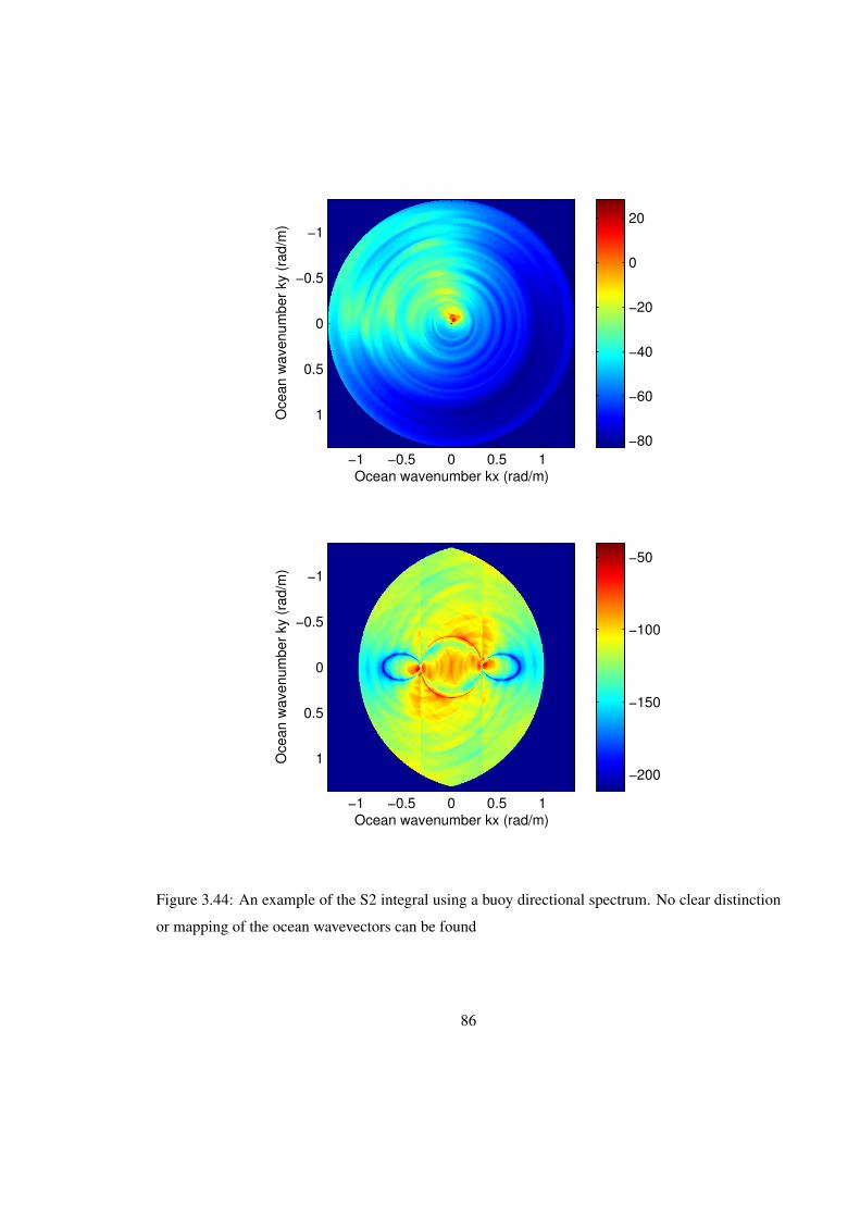
Ocean wavenumber kx (rad/m)
Ocean w
avenum
ber
ky (
rad/m
)
−1 −0.5 0 0.5 1
−1
−0.5
0
0.5
1
−80
−60
−40
−20
0
20
Ocean wavenumber kx (rad/m)
Ocean w
avenum
ber
ky (
rad/m
)
−1 −0.5 0 0.5 1
−1
−0.5
0
0.5
1−200
−150
−100
−50
Figure 3.44: An example of the S2 integral using a buoy directional spectrum. No clear distinction
or mapping of the ocean wavevectors can be found
86

0 0.5 1 1.5−40
−35
−30
−25
−20
−15
−10
−5
0
5
10
Doppler Frequency (Hz)
Weig
hting A
mplit
ude (
dB
)
Total Coefficient Γ
EM + Γ
H
Hydrodynamic Coefficient ΓH
Electromagnetic Coefficient ΓEM
Figure 3.45: The Doppler frequency-averaged Coupling coefficient. The total coefficient ΓT
[black], is shown with its contributions from EM term ΓEM [red] and hydrodynamic term ΓH
[blue]. The hydrodynamic 21/2fB and EM 23/4fB contributions remain, despite their decay to zero
for some directions.
87
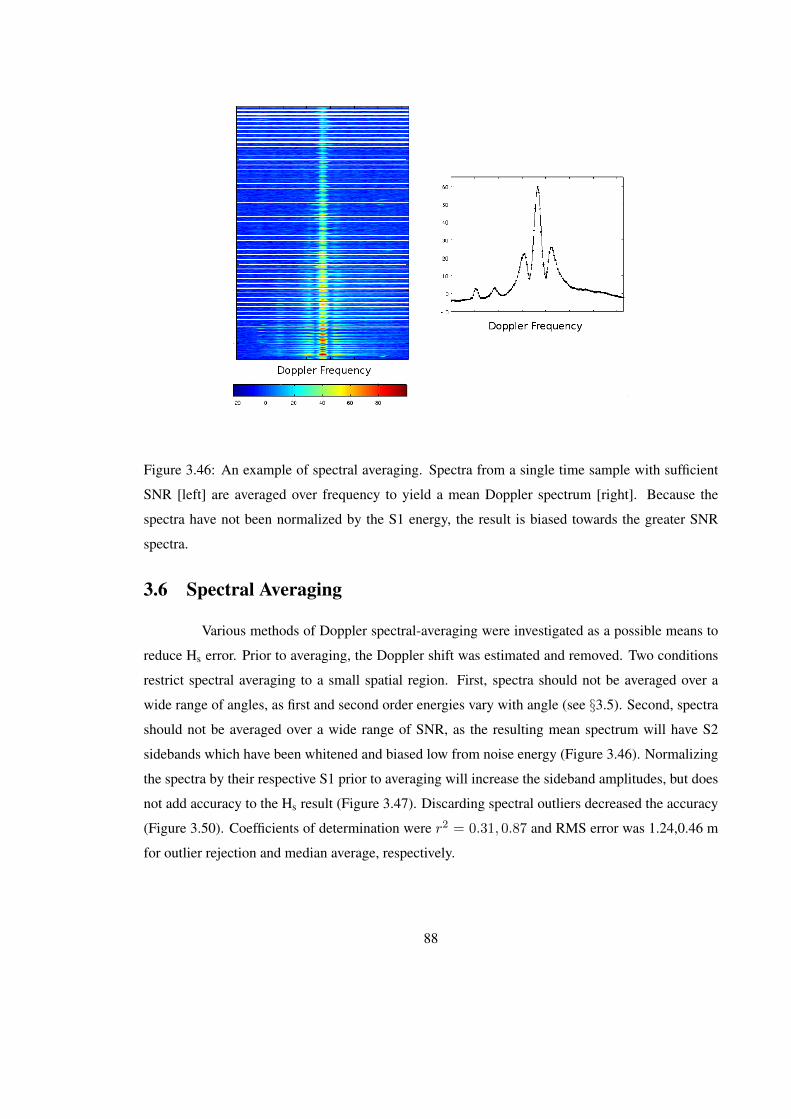
Figure 3.46: An example of spectral averaging. Spectra from a single time sample with sufficient
SNR [left] are averaged over frequency to yield a mean Doppler spectrum [right]. Because the
spectra have not been normalized by the S1 energy, the result is biased towards the greater SNR
spectra.
3.6 Spectral Averaging
Various methods of Doppler spectral-averaging were investigated as a possible means to
reduce Hs error. Prior to averaging, the Doppler shift was estimated and removed. Two conditions
restrict spectral averaging to a small spatial region. First, spectra should not be averaged over a
wide range of angles, as first and second order energies vary with angle (see §3.5). Second, spectra
should not be averaged over a wide range of SNR, as the resulting mean spectrum will have S2
sidebands which have been whitened and biased low from noise energy (Figure 3.46). Normalizing
the spectra by their respective S1 prior to averaging will increase the sideband amplitudes, but does
not add accuracy to the Hs result (Figure 3.47). Discarding spectral outliers decreased the accuracy
(Figure 3.50). Coefficients of determination were r2 = 0.31, 0.87 and RMS error was 1.24,0.46 m
for outlier rejection and median average, respectively.
88

Figure 3.47: Example spectrogram normalized by S1 energy. Spectra are from a single time sample.
Spectral frequencies below the noise floor have been removed. Noise energy persists at the farthest
ranges due to variance about the mean noise level. The y-axis corresponds roughly to increasing
range.
89

Figure 3.48: A close-up of a spectrogram normalized by S1 energy. Spectra below a threshold SNR
have been removed. Strong S2 sidebands and S1:S2 nulls are evident in most spectra. Multiple
spurious noise peaks exist for some S2 sidebands.
Averaging spectra which exceed a threshold SNR did not improve the Hs estimate. The
mean spectra were contaminated by strong noise peaks(Figure 3.48). The Bragg peak had relatively
little amplitude variation. Iteratively discarding large variation (3σ) spectral outliers improved the
form of the sidebands; retaining physical features while discarding noise peaks (Figure 3.49). Al-
though this method produced visually improved spectra, Hs accuracy did not increase.
Spectral averaging was used to investigate the time evolution of the Doppler spectra. The
sidebands exhibited low-frequency peaks moving towards higher frequencies with time, analogous
to the arrival of distant swell (Figure 3.51). Following scattering theory, the frequency difference
between first and second order peaks decreased for more energetic swell.
90
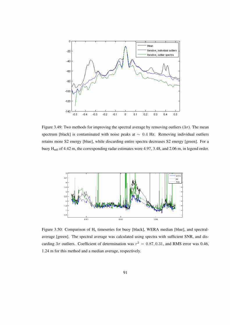
Figure 3.49: Two methods for improving the spectral average by removing outliers (3σ). The mean
spectrum [black] is contaminated with noise peaks at ∼ 0.4 Hz. Removing individual outliers
retains more S2 energy [blue], while discarding entire spectra decreases S2 energy [green]. For a
buoy Hm0 of 4.42 m, the corresponding radar estimates were 4.97, 3.48, and 2.06 m, in legend order.
Figure 3.50: Comparison of Hs timeseries for buoy [black], WERA median [blue], and spectral-
average [green]. The spectral average was calculated using spectra with sufficient SNR, and dis-
carding 3σ outliers. Coefficient of determination was r2 = 0.87, 0.31, and RMS error was 0.46,
1.24 m for this method and a median average, respectively.
91

Figure 3.51: Time evolution of spectra, showing improvement to the spectral mean by removing
spectral outliers. The mean spectrum [left] is contaminated with noise peaks at ± 0.4 Hz. After
removing outliers [right], time-varying characteristics of the S2 region are revealed.
92

Chapter 4
Discussion
4.1 Wind Estimates
The Bragg-ratio method of Long and Trizna [1973] has remained essentially unmodified
since its inception, although debate over the directional spreading model continues. Its utility for
physical analysis is somewhat reduced because it can not estimate wind magnitude. A possible
method for adding magnitude to the wind estimates would require inferring the ocean Bragg wave
amplitudes from the Doppler spectra (see Eqn. A.4.5), and entering these into an appropriate wind-
wave model. Inference of Bragg wave amplitudes from the second order spectrum would require
inversion of the second order integral equation. Provided the Bragg wave amplitudes could be
reasonably estimated, considerations must be made for growth and response times due to changing
winds [Masson, 1990].
Complex correlation between radar and modeled wind directions was quite poor. Con-
versely, radar wind directions were highly correlated (r2 = 0.83) to QuickSCAT measurements.
Agreement between these two empirical measurements is additional validation of the Long and
Trizna [1973] wind direction method. The bimodal wind fields observed in the radar measurements
are interesting features warranting further investigation.
Further analysis of the radar wind fields must take consideration for the imposed direc-
tional spreading function, and the limited dynamic range of observable Bragg ratios, which constrain
the measurable angles. This effect has been noted by previous researchers [Maresca and Georges,
1980, Harlan and Georges, 1994, Wyatt, 2001, Gurgel et al., 2006], and was observed in this study.
For winds nearly parallel to the radar beam, the radar-to-wind angle exceeds it measurable range
and a discontinuity in the spatial field is created. An algorithm is necessary which accounts for this
expected discontinuity without introducing a directional bias.
93

4.2 Significant Waveheight Estimates
Theoretical and observational analysis shows the Hs equation is inaccurate for k0hrms <
0.1 [Barrick, 1977]. Combining the upper and lower validity limits gives 0.1 < k0hrms < 4. Hs
observations from this study varied from 0 to 5 m, and were thus within the constraints of theoretical
validity. For the HOME radar, the lower limit of theoretical validity was 0.5 m.
Correlation analysis between the Waimea buoy and the radar-derived Hs showed external
interference as the primary cause for radar Hs error. The lower SNR of the second order region
reduces the wave measurements to 50% of the range for current measurements. Station-averaging
Hs estimates with varying SNR created spatial discontinuities in accuracy unsuitable for further
analysis. Removing low SNR data was shown to improve correlation and RMS error. Maximum
accuracy did not correspond with maximum SNR, possibly due to non-linear effects in the radar
receivers for the nearest range cells. Poor correlation at outermost angles of the measurement field
may be attributed to decreased beamforming directionality, i.e. wider centerlobes and greater side-
lobes. A variety of different averaging and filtering methods were unsuccessful at improving Hs
accuracy.
The decreasing frequency separation for first and second order peaks is a possible expla-
nation for additional error in Hs estimation. Peak second order values occur closest to the Bragg
peak, and move closer to the Bragg peak for lower frequency peak ocean swell [Barrick, 2005a]. An
instrumental limit is reached when the S1:S2 separation is less than the spectral resolution (which
will exceed df due to spectral filters). At this limit, the S1 and S2 energies are convolved, causing
Hs to be underestimated by biasing the S2/S1 ratio towards unity. This effect explains the observed
underestimation of Hs at large Hs (Figure 4.1). For this experiment, the saturation limit was Hs =
11.9 m, whereas S1:S2 merging was possibly observed at 4 m. This suggests the merging is due to
spectral resolution, and not a physical limitation of the radar. Further evidence of S1:S2 merging is
the under-estimation of Hs for peak swell in the timeseries.
Evaluation of the S2 integral equation showed the coupling coefficient varied significantly
with direction. Previous researchers have concluded the Hs equation is insensitive to direction
[Barrick, 1977, Maresca and Georges, 1980]. Although, their evaluations were based on synthetic
wave models with symmetric directional spread and no representation for multi-mode seas. Barrick
[1977] estimated the error associated with the assumption of a mean coupling coefficient on the
order of 15%. Both researchers noted increased Hs error for k0h < 0.3 m. This suggests the
94
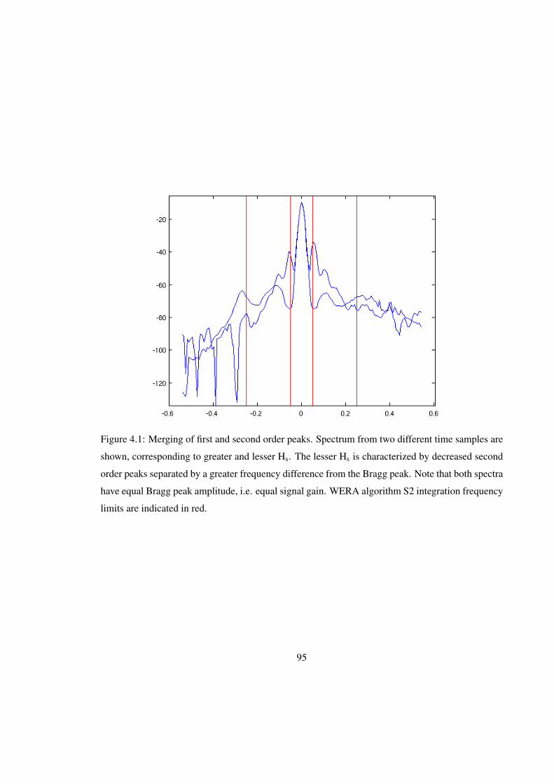
Figure 4.1: Merging of first and second order peaks. Spectrum from two different time samples are
shown, corresponding to greater and lesser Hs. The lesser Hs is characterized by decreased second
order peaks separated by a greater frequency difference from the Bragg peak. Note that both spectra
have equal Bragg peak amplitude, i.e. equal signal gain. WERA algorithm S2 integration frequency
limits are indicated in red.
95

coupling coefficient becomes more directionally dependent for higher ocean frequencies. Maresca
and Georges [1980] noted poor accuracy for highly directional spectra.
The S2 integral summation frequencies approach a nearly linear relation to ocean wavenum-
ber for k > 1.5 rad m−1, corresponding to Doppler frequencies |ωD| > 1.5 Hz. The frequencies
are far outside the significant contribution to second order energy. This raises questions about the
theoretical validity of empirical fits between the scalar ocean spectrum and the Doppler spectrum,
as used in the WERA algorithm. The energetic lower Doppler frequencies are integrals over a large
range of ocean wavenumber and direction. Theoretical work by Barrick [1972], Weber and Barrick
[1977], Barrick and Weber [1977] has shown this simple proportionality to be incorrect. Further-
more, linear regression between the Doppler spectrum and ocean spectrum is unlikely to resolve
or correct the following observed second-order coupling coefficient features; 21/2fB hydrodynamic
peak, 23/4fB EM peak, and exponential gain with higher Doppler frequency.
——————-
Previous researchers have also encountered significant, sometimes limiting, Hs error due
to RFI noise. Wyatt and Green [2002] reported significant decrease in spatial and temporal coverage
due to RFI. Despite highly directional RFI, the SNR was reduced in all directions. Wyatt et al.
[2006] concluded the OSCR radar data had insufficient quality for wave measurements, due to low
SNR and antenna sidelobes.
RFI noise creates spurious signals due to its additive effect. These signals can either
deform or completely mask the desired ocean signal. Previous researchers have noted the difficulty
in recovering usable first or second order ocean signal in the presence of RFI noise [Gurgel et al.,
2006, Gurgel and Barbin, 2008]. Accuracy, range, and temporal coverage are all reduced.
The assumption of Rayleigh distributed noise compared well with observations. Fitting
a Rayleigh distribution to the ordered spectral energies is shown to perform significantly better
at estimating the mean noise value than a simple mean over a smaller range of frequencies. The
Rayleigh regression resulted in percent errors of 0.01%. Although, this level of accuracy for the
noise estimate is unwarranted, as the noise amplitude does not enter into the equations for ocean
parameters. Rather, it is used as a quality control parameter, and in this context high accuracy is not
needed. Ordered statistics is most useful when the Doppler spectra is a combination of white noise
and relatively greater narrow band sources, e.g. RFI, power supply, or ship echoes. The ordered
statistics method is capable of separating the two sources using the energy distribution.
Inspection of the noise level estimates yielded a background noise level of ∼ −80 dB,
with peak values of∼ −45 dB. The primary contribution to the noise field was external interference.
96

Both stations identified the strongest source at a heading of 201, with similar amplitude sources
from other headings. A simple mathematical modelN = NI(r)+NE(θ, t) described the noise as a
function of range, angle, and time. The constant range-decay termNI(r) was relatively insignificant
compared to the directional external interferences NE(θ, t). These external interferences had a
strong diurnal cycling attributed to greater human activity during daylight hours and sun-driven
ionospheric cycles.
Spectral, i.e. frequency, averaging was evaluated for improving Hs estimates without
success. Because S1 and S2 vary with direction, spectral averaging should only be done for θ 'constant. The effect of averaging spectra with varying SNR was shown to bias the Hs estimate high
due to the integration of noise energy in S2. Thus spectra should only be averaged over a narrow
angle and range.
Neither eigen-decomposition or a simple model based approach were successful in re-
ducing the RFI. Eigen-decomposition was not capable of representing the RFI in a few energetic
modes. Furthermore, the RFI and ocean signal were not separated in eigenspace, preventing removal
of specific modes. A plausible explanation is that the ocean scatter does not have a coherent signal
across either antenna or range. Thus it randomly maps into the coherent modes of RFI. For eigen-
decomposition to work, the the majority of the RFI energy must map into only a few independent
eigenmodes. It is questionable if the assumption of orthogonality is appropriate for representing
RFI signals.
The model based approach of estimating the RFI sinusoids showed some promise. The
RFI energy was entirely rejected in a narrow range band. Rejection of RFI energy for all ranges was
not possible due to errors in estimating the RFI phase. The assumption of a constant RFI frequency
in the model is the most likely explanation. Clearly, most anthropogenic signals will have frequency
modulation on a scale similar to the FMCW modulation. Additional phase models would be worth
pursuing. A fundamental problem with the model-based method is it introduces erroneous energy
if the RFI phase is not accurately estimated.
There are alternative solutions for reducing RFI not examined in this thesis. One proactive
method is to dynamically choose an unused HF bandwidth to operate the radar. Gurgel and Barbin
[2008] discusses adaptive bandwidth allocation with ambient monitoring. In some situations, quiet
channels may not be found. Linear prediction filtering may be used to remove the impulse noise of
RFI from the time domain [Ponsford et al., 2003]. Linear prediction requires a relatively large ratio
of clean, i.e. RFI-free, samples to work. The RFI observed in this thesis was the dominant feature
in both the time and frequency domain. Adaptive beamforming is another well-developed method
97

for canceling point-sourced RFI [Molnar et al., 1990], wherein noise sources are minimized via the
principle of interference and carefully chosen filters.
98

Chapter 5
Conclusion
With proper calibration and data processing, oceanographic radar is capable of providing
wide-area measurements that are difficult or impossible to make any other way. The theory and
operation of oceanographic radars has been discussed and evaluated. Much of the analysis in this
thesis has focused on errors and uncertainties in the radar-derived Hs measurement. All measure-
ments, in-situ or remotely-sensed, have uncertainties and associated error due to the relationship
between physical process and sensor. In the case of second-order EM scattering from the sea sur-
face, the theoretical relationship is fairly well understood. Because the interaction mechanism is
second-order, direct unambiguous measurement of a specific ocean wavelength is not possible.1
Rather, integrated properties such as Hs, mean period, and mean direction are estimated.
The first and second order EM-ocean interaction mechanisms are separated by how the
information content is encoded in the radar signal. First order scattering carries ocean surface veloc-
ity information in the Doppler frequency, and is a relatively robust measurement. The Bragg peak
occupies a narrow frequency bandwidth and is consequently less likely to share noise frequencies.
Conversely, second order scattering is an amplitude based measurement over a comparatively large
frequency bandwidth, making it far more susceptible to external interference. Accuracy of the Hs
estimate was shown to be dependent on a sufficiently high signal-to-noise ratio. Insufficient SNR
results in biasing of the S2 energy by the mean noise level. The effect of the bias depends on the
noise conditions. For a quiescent noise environment, i.e. primarily thermal noise, the Hs estimate is
biased low. For RFI-dominated conditions, the Hs estimate is biased high with excessive variation.
In this thesis and much of the literature, the removal of RFI from data is a difficult task
which may not be fully possible. To this end, two suggestions are made. Reduce the amount of RFI
by monitoring the radio frequency environment and selecting unoccupied bandwidths, e.g. Gurgel1Caveats to this statement are the 21/2fB and 23/4fB singularities.
99
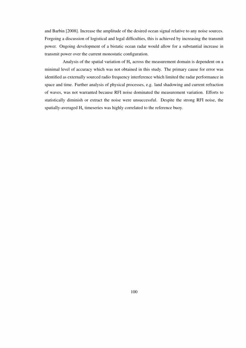
and Barbin [2008]. Increase the amplitude of the desired ocean signal relative to any noise sources.
Forgoing a discussion of logistical and legal difficulties, this is achieved by increasing the transmit
power. Ongoing development of a bistatic ocean radar would allow for a substantial increase in
transmit power over the current monostatic configuration.
Analysis of the spatial variation of Hs across the measurement domain is dependent on a
minimal level of accuracy which was not obtained in this study. The primary cause for error was
identified as externally sourced radio frequency interference which limited the radar performance in
space and time. Further analysis of physical processes, e.g. land shadowing and current refraction
of waves, was not warranted because RFI noise dominated the measurement variation. Efforts to
statistically diminish or extract the noise were unsuccessful. Despite the strong RFI noise, the
spatially-averaged Hs timeseries was highly correlated to the reference buoy.
100

Appendix A
Electromagnetic Scattering Derivations
This appendix is intended as a convenient summary and reference to Barrick’s derivations
of electromagnetic scattering from the ocean surface. The reader is referred to the original publica-
tions for completeness [Barrick, 1970, 1971a,b, 1972, Derr, 1972, Weber and Barrick, 1977, Barrick
and Weber, 1977].
A.1 Ground Wave Propagation
Barrick [1970] investigated the attenuation of a vertically polarized EM ground-wave due
to sea surface roughness. The sea surface roughness causes a scattered EM field, which Barrick
[1970] represents as a summation of modes in the total EM field. The strength of the scattered EM
modes are directly proportional to the ocean wave modes. The equations result in both propagating
and evanescent modes, separated by the Bragg wavelength of the scatterers. Only ocean waves
longer than the Bragg wavelength contribute to the resistive portion (Figure A.1). These longer
waves are responsible for the removal of energy from the guided waves and scatter into all directions
in the upper hemisphere [Barrick, 1970]. Oceans waves of less than the Bragg wavelength result
in inductive reactance, and do not scatter the EM wave. Rather, they produce a perturbation on the
local field at the surface that does not propagate, and exists only near the region between the waves,
i.e. evanescent [Barrick, 1970].
Barrick [1970, 1971b] numerically investigated the attenuation of an EM ground-wave
as a function of sea state, transmit frequency and antenna height above the sea surface using a
standard ESSA Fortran ground-wave program. Semi-empirical wind-wave models were used as
inputs (Neumann-Pierson and [Phillips, 1958]). Attenuation increased with sea state, higher EM
frequencies, and longer ranges [Barrick, 1971b]. Attenuation due to sea state was small compared
to background loss, i.e. for a smooth sea. For example, the attenuation due to a smooth sea was
101
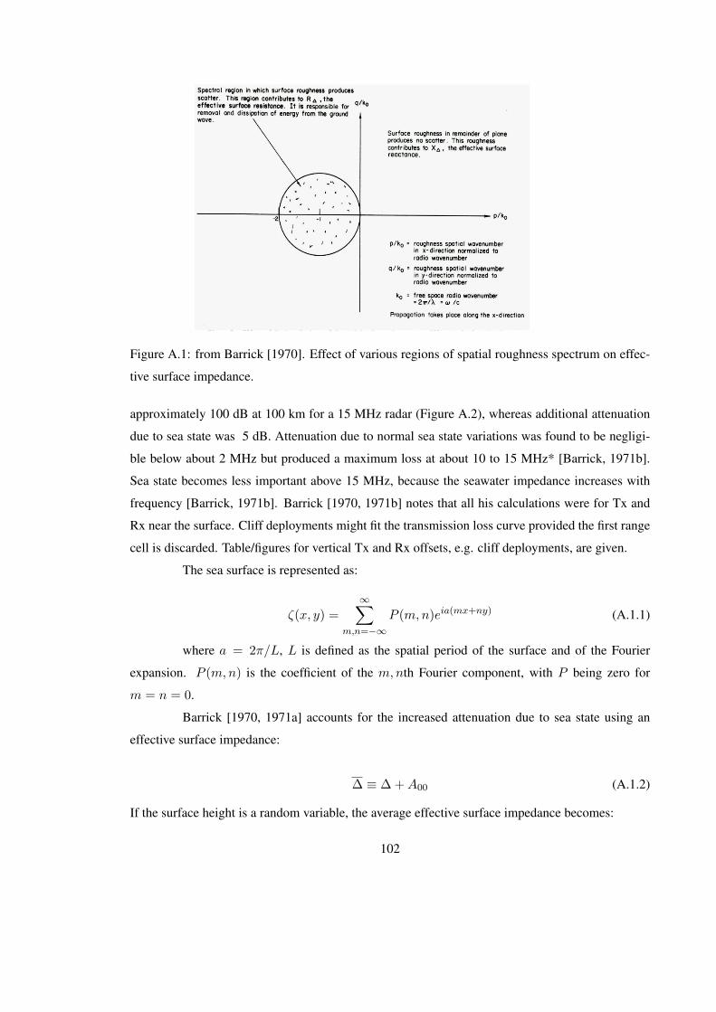
Figure A.1: from Barrick [1970]. Effect of various regions of spatial roughness spectrum on effec-
tive surface impedance.
approximately 100 dB at 100 km for a 15 MHz radar (Figure A.2), whereas additional attenuation
due to sea state was 5 dB. Attenuation due to normal sea state variations was found to be negligi-
ble below about 2 MHz but produced a maximum loss at about 10 to 15 MHz* [Barrick, 1971b].
Sea state becomes less important above 15 MHz, because the seawater impedance increases with
frequency [Barrick, 1971b]. Barrick [1970, 1971b] notes that all his calculations were for Tx and
Rx near the surface. Cliff deployments might fit the transmission loss curve provided the first range
cell is discarded. Table/figures for vertical Tx and Rx offsets, e.g. cliff deployments, are given.
The sea surface is represented as:
ζ(x, y) =
∞∑m,n=−∞
P (m,n)eia(mx+ny) (A.1.1)
where a = 2π/L, L is defined as the spatial period of the surface and of the Fourier
expansion. P (m,n) is the coefficient of the m,nth Fourier component, with P being zero for
m = n = 0.
Barrick [1970, 1971a] accounts for the increased attenuation due to sea state using an
effective surface impedance:
∆ ≡ ∆ +A00 (A.1.2)
If the surface height is a random variable, the average effective surface impedance becomes:
102
Figure A.2: from Barrick [1971b]. Basic transmission loss across the ocean between points at the
surface of smooth spherical Earth. Conductivity is 4 mhos/m and an effective Earth radius factor of
4/3 is assumed.
∆ ≡ 〈∆ +A00〉 = ∆ + 〈A00〉 (A.1.3)
Following a standard perturbation approach, the solution for 〈A00〉 to second order is given in
Barrick [1970, 1971a, Eq.11,Eq.24]:
∆ = ∆ +1
4
∫ ∞−∞
∫ ∞−∞
F (p, q)W (p, q)dpdq (A.1.4)
where
F (p, q) =p2 + b′∆(p2 + q2 − k0p)
b′ + ∆(b′2 + 1)+ ∆(
p2 − q2
2+ k0p)b
′ =1
k0
√k2
0 − (p+ k0)2 − q2
(A.1.5)
where W (p, q) is the ocean wave spectrum.
A.2 Ground Wave Scatter
The random sea surface is represented as a Fourier series in space and time, and first-order
expressions are derived for the received Doppler spectrum. The scattered EM field is represented
103

as a Fourier series, with the solution coefficients representing modes of the scattered field. The
previous section (Ground Wave Propagation) discussed how the scattered modes can be propagating
or non-propagating (Figure A.1). Barrick [1970, 1972] emphasizes the importance of the EM field
coefficients: ”The direction of propagation of the scattered mode is directly related to the Fourier
component of the surface, and for propagation modes, this direction is the Bragg direction required
by a periodic surface with wavenumbers am and an.”
Barrick [1970, 1972] derived the scattered EM field using a perturbation method [Kline,
1951] and boundary conditions at the surface. Necessary assumptions for the perturbation method
include; 1) the sea surface height, ζ, above a mean plane is small in terms of the EM wavelength;
and 2) the sea surface slope,∇ζ, is small for these longer ocean waves. The Leontovich impedance
boundary condition requires 3) the ocean-water medium is highly conducting. For HF, condition
1) is met by ocean waves, and condition 3) is met by seawater [Barrick, 1970, 1972]. Condition 2)
becomes an operational limitation and is discussed in §2.2. Limits on the mathematical validity of
the solution are given in terms of frequency and sea state [Barrick, 1972, pg.7].
The following derivations are taken directly from [Barrick, 1970]. They illustrate how the
received Doppler spectrum is derived from electromagnetic and hydrodynamic first-principles.
The sea surface height is expressed as a Fourier expansion in space and time:
ζ(x, y, t) =
∞∑m,n,l=−∞
P (m,n, l)eia(mx+ny)−iwlt (A.2.1)
where a = 2π/L, w = 2π/T , L and T are defined as the spatial and temporal periods of the surface
and of the Fourier expansion. P (m,n) is the coefficient of the m,nth Fourier component, with P
being zero for m = n = 0.
Following Kline [1951] define an average spatial-temporal spectrum W (p, q, ω) of the
surface height in terms of the Fourier coefficients as
W (p, q, ω) =1
π3
∫∫∫ ∞−∞〈ζ(x1, y1, t1)ζ(x2, y2, t2)〉eipτx+iqτy−iωτdτxdτydτ =
L2T
π3〈P (m,n, l)P (−m,−n,−l)〉 (A.2.2)
where 〈P (m1, n1, l1)P (m2, n2, l2)〉 is zero whenm2 6= −m1,n2 6= −n1, and l2 6= −l1 because the
Fourier coefficients are uncorrelated. Also, p = am, q = an, ω = wl, τx = x2 − x1, τy = y2 − y1,
and τ = t2 − t1. The angular braces denote a statistical ensemble average. Also, 〈P (m,n, l)〉 = 0
for all m,n, l.
104
The perturbed electric fields arising from a vertically polarized wave at grazing incidence
passing over the surface are represented as:
Ex = ∆E(h, 0, z, l) +∞∑
m,n,l=−∞AmnlE(m+ h, n, z, l) (A.2.3)
Ey =∞∑
m,n,l=−∞BmnlE(m+ h, n, z, l) (A.2.4)
Ez = E(h, 0, z, l) +
∞∑m,n,l=−∞
CmnlE(m+ h, n, z, l) (A.2.5)
E(m+ h, n, z, l) = E0ei(a(m+h)x+any+b(m+h,n)z+(wl−ω0)t) (A.2.6)
b(m+ h, n) =√k2
0 − a2(m+ h)2 − a2n2 (A.2.7)
where h = k0 sin θi/a. The definition of b above is such that A.2.3 satisfy the Helmholtz wave
equation. The magnetic fields H are not given, but are determined from Maxwell’s equations.
From A.2.3, the electric field E is complex in general so it has a magnitude and a phase. ∆ is
the normalized surface impedance at grazing for a medium below the smooth interface of complex
permittivity ε1 and permeability µ1
∆ =1
120π
õ1
ε1×√
1− ε0µ0
ε1µ1' 1
120π
õ1
ε1for ε1 ε0 (A.2.8)
Included in ε1 is the effect of conductivity, i.e. ε1 = εr1 + iσ1/ω0, where εr1 is the real dielectric
constant of the medium and σ1 is it conductivity. For sea water at 10 MHz, for example, εr1 ' 80ε0,
σ1 ' 4 mhos/m, ε1 ' ε0(80 + i7200), and ∆ ' 1.18 · 10−2 exp−iπ/4.
The solution of the problem consists of finding Amnl, Bmnl, Cmnl. This is done using the
Kline [1951] perturbation expansion with Leontovich boundary conditions at the surface. Only first
order terms are retained. The solution for the coefficients is:
Amnl =NA
D(m,n)P (m,n, l) (A.2.9)
Bmnl =NB
D(m,n)P (m,n, l) (A.2.10)
Cmnl =−a[(m+ h)NA − nNB]
b(m+ h, n)D(m,n)P (m,n, l) (A.2.11)
105
where
NA = −iam[1 +∆k0
b(1− a2(m+ h)2
k20
)] + ian∆k0
b
a2n(m+ h)
k20
(A.2.12)
NB = −ian[1 +∆k0
b(1− a2n2
k20
)] + iam∆k0
b
a2n(m+ h)
k20
(A.2.13)
D(m,n) ' 1 +∆k0
b(m+ h, n)(1 +
b2(m+ h, n)
k20
) (A.2.14)
Again: the first-order coefficients of the scattered EM mode are directly related to the
Fourier coefficients of the surface mode, e.g. Amnl = NAD(m,n)P (m,n, l). The direction of prop-
agation for the EM mode being the same as the Bragg wavenumber of the surface m,n mode, i.e.
kB = 1/2(mx+ ny).
A.3 Far Field Scatter
Thus far, Barrick [1970] has derived modal, plane-wave expansions A.2.3,A.2.9 for the
scattered EM fields above a surface of infinite extent, given the Fourier expansion of the surface.
Barrick [1970] proceeds to derive an expression for the received EM field at a distant antenna.
The analysis begins with a previously derived [Ruck et al., 1970] expression for the scattered mag-
netic far-field A.3.1, which is a function of the electric and magnetic fields at a point (Figure ref-
fig:barrick:1970:3). This vector integral is obtained using the vector analog of Green’s Theorem
on Maxwell’s equation [Ruck et al., 1970]. It is often called the Chu-Stratton integral, and un-
der simplifying assumptions, the physical optics integral. Thus the EM far-field is derived from
electromagnetic first principles.
Consider a patch of sea surface dS of finite extent. Choose a square patch of side L,
with the condition that L is much larger than the wavelength λ but much smaller than R0 the
distance from the patch to the observation point, i.e. λ L R0. When the scattering patch is
considerably smaller in extent than R0 (Figure 1.8), we can employ the following equation for the
scattered magnetic field [Ruck et al., 1970]:
Hs(R0, t) '
ik0eik0R0
4πR0
∫ L/2
−L/2
∫ L/2
−L/2[ks0× (z×Hs)−
√ε0µ0
(z×Es) +
√ε0µ0ks0 · (z×Es)ks0]e−ik0k
s0·r′dxdy
(A.3.1)
106
whereEs andHs in the integrand are the fields evaluated at the surface element dxdy on the z = 0
plane. Hs is determined from Es using Maxwell’s equations. The vector r′ points from the origin
to the local area increment, dxdy, on the surface of integration, i.e. r′ = xx + yy + zz. ks0 is a
unit vector pointing in the desired observation direction, i.e. ks0 = sin θs cosφsx+ sin θs sinφsy +
cos θsz (Figure 1.8).
For the scattered H-field normal to the scatter plane, i.e. the ϕs component ofHs(R0, t),
the integral becomes:
Hsϕ(R0, t) =
ik0eikoR0
4πR0
∑m,n,l
∫ L/2
−L/2
∫ L/2
−L/2fϕ(m,n)P (m,n, l)
ei(a(m+h)x+any+(wl−ω0)t)e−ik0(sin θs cosϕsx+sin θs sinϕsy)dxdy (A.3.2)
where fϕ(m,n) is a factor containing NA,NB , and ks0, determined from A.3.1.
A.3.2 can be integrated over the square patch to give:
Hsϕ(R0, t) =
ik0eik0R0
πR0
∑m,n,l
fϕ(m,n)P (m,n, l)
[sin L
2 (a(m+ h)− k0 sin θs cosϕs)
a(m+ h)− k0 sin θs cosϕs
][sin L
2 (an− k0 sin θs sinϕs)
an− k0 sin θs sinϕs
]ei(wl−ω0)t (A.3.3)
Barrick then proceeds to show how the effective surface impedance ∆ is accounted for
Barrick [1970, see §3.3]. In short, the solution is found by evaluating the scattering equation for
zero impedance ∆ = 0, and multiplying by the Norton attenuation factor 2F ′. The only factor
affected by this step is fϕ.
A.4 Average Scattered Signal Spectrum
At this point, we are ready to consider averaging over ensembles of surfaces whose
Fourier expansion coefficients P (m,n, l) are random variables. To this end, form Hsφ(R0, t1)Hs
φ ∗(R0, t2) from A.3.3 and average to obtain Rs(τ), where τ = t1 − t2. This implies stationarity in
the temporal sense so that Rs(τ) depends only on the difference, τ , and not upon t1 or t2.
107
Rs(τ) =k2
0L4F ′2
32π2R20
∫ ∫ ∫ ∞−∞
∣∣f cϕ(p, q)∣∣2[
sin L2 (k0 sin θs cosϕs − k0 − p)
L2 (k0 sin θs cosϕs − k0 − p)
]2 [sin L
2 (k0 sin θs sinϕs − k0 − q)L2 (k0 sin θs sinϕs − k0 − q)
]2
W (p, q, ω)ei(ω−ω0)τdpdqdω
(A.4.1)
where f cϕ is fϕ evaluated at ∆ → 0. The six summations have been reduced to the triple integral
by using the statistical independence of the Fourier coefficients and the definition of the spatial
and temporal surface height spectrum A.2.2. Since all quantities in the integrand now apply to a
perfectly conducting surface, ah becomes k0 Barrick [1970].
Equation A.4.1 is simplified by employing the previous assumption that the scattering
patch size L is much greater than the wavelength, so that k0L >> 1. Under these conditions, the
[sinx/x]2 functions in the integrand become impulse functions:
L
[sin L
2 (k0 sin θs cosϕs − k0 − p)L2 (k0 sin θs cosϕs − k0 − p)
]2
⇒ 2πδ[p− k0(sin θs cosϕs − 1)] (A.4.2)
This simplification is key, because the impulse function reduces the integral over all wavenumbers
to only those satisfying the Bragg wavelength. These impulse functions permit integration of A.4.1
over p and q to give
Rs(τ) =k2
0L2F ′2
8R20
[f cϕ(k0(sin θs cosϕs − 1), k0 sin θs sinϕs)
]2∫ ∞−∞
W (k0(sin θa cosϕs − 1), k0 sin θs sinϕs, ω)ei(ω−ω0)τdω (A.4.3)
The power density spectrum of the scattered signal is the Fourier transform of the correlation func-
tion:
P s(ω) =1
π
∫ ∞−∞
Rs(τ)e−iωτdτ
=k2
0L2F ′2
4R20
[f cϕ(k0(sin θs cosϕs − 1), k0 sin θs sinϕs)
]2W (k0(sin θs cosϕs − 1), k0 sin θs sinϕs, ω − ω0) (A.4.4)
108

Now simplify f cϕ by noting that as ∆ → 0,NA → −ip = −ik0(sinθs cosϕs − 1),NB → −iq =
−ik0 sin θs sinϕs, and D(m,n)→ 1.
P s(ω) =k4
0L2F ′2H2
0
4R20
(sinθs−cosϕs)2W (k0(sin θs cosϕs−1), k0 sin θs sinϕs, ω−ω0) (A.4.5)
where H0 = k0ω0µ0
E0. Convert to σ(ω), the range-independent bistatic scattering cross section per
unit surface area per radian s−1 bandwidth by multiplying by 4πR2/L2H20F′2 to obtain:
σ(ω) = πk40(sin θs − cosϕs)
2W (k0(sin θs cosϕs − 1), k0 sin θs sinϕs, ω − ω0) (A.4.6)
Integrate over all frequencies to obtain the average bistatic scattering cross section per unit area:
σ0 = πk40(sin θs − cosϕs)
2W (k0(sin θs cosϕs − 1), k0 sin θs sinϕs) (A.4.7)
Both spectra have the wavenumbers p, q replaced by k0(sin θs cosφs− sin θi), k0 sin θs sinφs. The
latter are precisely the wavenumbers required of a diffraction grating which is to scatter a wave
incident from θi into directions θs, φs.
A.5 First Order Spectrum
This section applies the gravity wave dispersion relation to simplify 1.4.2 and yield the
final first order relationship between the ocean wave directional spectrum and Doppler spectrum
1.4.5. The derivation is from Barrick [1970, 1972].
The first-order surface gravity wave dispersion relation makes it possible to relate the
spatial-temporal height spectrum W (p, q, ω) to the simpler spatial spectrum W (p, q).
ω2g± = ±g
√p2 + q2 = ±g
√(am)2 + (an)2 (A.5.1)
Therefore, A.2.1 is rewritten as follows:
ζ(x, y, t) =
∞∑m,n=−∞
P±(m,n)ei(amx+any+ωg±) (A.5.2)
The spatial-temporal spectrum then becomes:
109

W (p, q, ω) = 2W+(p, q)δ(ω + ω+) + 2W−(p, q)δ(ω + ω−) (A.5.3)
where W±(p, q) = 〈|P±(m,n)|2〉L2/π2, the ± signs refer to the direction of motion of the waves,
and ω± is given in 1.4.3.
The spatial-temporal waveheight spectrum for a given p,q (spatial wavenumbers) consists
of only two possible discrete temporal frequencies, ω+ and ω−, which are related to p and q through
1.4.3 [Barrick, 1970].
Substituting 1.4.4 into 1.4.2:
σ(ω) = 4πk40(sin θs − cosϕs)
2 [W+(k0(sin θs cosϕs − 1), k0 sin θs sinϕs)δ(ω + ω+ − ω0)
+W−(k0(sin θs cosϕs − 1), k0 sin θs sinϕs)δ(ω + ω− − ω0)] (A.5.4)
A.6 Second Order Spectrum
The vertical displacement of the surface due to waves is represented as a spatial and
temporal Fourier series:
η(r, t) =∑k,ω
η(k, ω) exp i(k · r − ωt) (A.6.1)
where r = xx+ yy is the position in the x,y plane. The velocity potential is:
Φ(r, z, t) =∑k,ω
Φ(k, ω) exp kz + i(k · r − ωt) (A.6.2)
The fact that η(r, t) and Φ(r, z, t) are real physical quantities requires η∗(k, ω) = η(−k,−ω)
and Φ∗(k, ω) = Φ(−k,−ω). The Fourier coefficients for waveheight η(k, ω), velocity potential
Φ(k, ω) and frequency ω are expanded in perturbation series as follows:
η(k, ω) = η1(k, ω) + η2(k, ω) + ..., (A.6.3)
Φ(k, ω) = Φ1(k, ω) + Φ2(k, ω) + ..., (A.6.4)
ω = ω0 + ω1 + ω2 + ..., (A.6.5)
First order terms are equated to yield:
110

ω20 − gk (A.6.6)
At this point, the notation K,Ω is used for second order waves to indicate their exclusion from the
first order dispersion relation A.6.6. The spatial wavenumber of the second order wave K is the
vector sum of the wavenumbers of the first order waves present. The same is true for the frequencies.
K = k + k′ and Ω0 = ω0 + ω′0 (A.6.7)
(to lowest order, where ω0 =√gk and ω′0 =
√gk′). The second-order waveheight:
η2(K,Ω) =∑k,ω
∑k′,ω′
A(k, ω,k′, ω′)η1(k, ω)η1(k′, ω′)× δk+k′
K δω+ω′
Ω (A.6.8)
where the expression has been written in a symmetrical form with the help of the Kronecker delta
functions, and where
A(k, ω,k′, ω) =
12 [k + k′ +
ω0ω′0g (1− k · k′)(gK+Ω2
0
gK−Ω20)]
0 if k′ = −k and ω′ = −ω(A.6.9)
k and η1(k, ω are taken as the independent variables of the problem, and all other quantities are
dependent upon these variables. Thus, to lowest order ω ≈ ω0 as derived in A.6.6, and is seen to be
a function of k ≡ |k|. Therefore, η1 is actually only a function of k. The Kronecker deltas can be
removed from A.6.9, since they essentially express that frequency terms in the summations are not
independent variables, (functions of k), so the sums can be over k only.
The solution is then carried to third order to solve for the first nonzero correction to the
lowest order dispersion relation A.6.6. ω = ω0 + ω2. (ω1 = 0)
ω2 = ω0
∑k′,ω′
C(K, ω,k′, ω′)|η1(k′, ω′)|2 (A.6.10)
where
C(k, ω,k′, ω′) =1
2
[k′2 +
ω′0ω0k · k′(2 +
k
k′)
](1− 1
2δωω′δ
kk′ −
1
2δ−ωω′ δ
−kk′
)
+A(k, ω,k′, ω′)
[−k′ + ω′0
ω0
k · k′
k′
]−B(k, ω,k′, ω′)
iω0
[k · (k + k′)− k|k + k′|+ ω′0k
ωk′k′ · (k + k′)
](A.6.11)
111
where
B(k, ω,k′, ω′) =−iΩ0ω0ω
′0(1− k · k′)
gK − Ω20
(A.6.12)
The gravity wave dispersion relation can be expressed (to second order):
ω(k) = ω0 + ω2 = ω0(1 +ω2
ω0) =
√gk(1 +
ω2
ω0) (A.6.13)
and hence
vph =√gk(1 +
ω2
ω0) =
√gk(1 + ∆vph(k)) (A.6.14)
The waveheights η1(k, ω) are in general complex random variables whose statistics change
over areas and times larger that those required for energy transfer [Weber and Barrick, 1977]. The
analysis continues by performing statistical averaging of the Fourier series solutions; yielding aver-
age waveheight spectra.
Using statistical assumptions, the surface waveheight spectrum is defined in terms of the
height coefficients (for each order) as:
〈ηn(k, ω)η∗n(k′, ω′)〉 =
(2π)3
LxLyTSn(k, ω) for k′ = k and ω′ = ω
0 for other k′,ω′(A.6.15)
where 〈f〉 denotes an ensemble average of f , and Sn(k, ω) is the nth order directional waveheight
spectrum for arbitrary spatial wave vector K and frequency ω. The waveheight coefficients are
taken to have zero mean: 〈η1(k, ω)〉 ≡ 0 for all k,ω.
The waveheight spectra are defined with the following normalization with respect to root-
mean-square waveheight h:
h2 = 〈η2(r, t)〉 =
∫ ∞−∞
∫ ∞−∞
d2k
∫ ∞−∞
dωS(k, ω) (A.6.16)
The periodic, nonrandom, Fourier series descriptions of waves A.6.8 is converted to in-
tegrals representing average spectra. Using A.6.8, an expression for the second order waveheight
spectrum S2(K,Ω) is derived in terms of the first order waveheight spectra:
S2(K,Ω) =1
2
∫ ∞−∞
∫ ∞−∞
d2κ∑u,l
∑u,l
A2(k,±√gk,k′,±
√gk′)S1(±k)S1(±k′)δ(Ω∓
√gk∓
√gk′)
(A.6.17)
112
σ2(ωd) = 24πk40
∫ ∫ ∞−∞|Γ( ~k1, ~k2)|2S( ~k1)S( ~k2)δ(ωd − ω1 − ω2)d~k (A.6.18)
where k ≡ 1/2K + κ, k′ ≡ 1/2K − κ, and the summation indices refer to the upper and lower
signs in the equation. The Dirac-delta function permits evaluation of one integral, leaving the other
to be done numerically.
Defining the mean wave frequency in a centroid sense:
ω =
∫∞0 ωS(ω)dω∫∞0 S(ω)dω
(A.6.19)
The radar mean wave period τ0 is [Barrick, 1977]:
ωBτ0
2π=
∫ 1,∞0,1 σ2(ωBν)/W (ν)dν∫ 1,∞
0,1 |ν − 1|σ2(ωBν)/W (ν)dν(A.6.20)
where the integrations could be over [0,1] or [1,∞].
113
Appendix B
WERA Significant Waveheight
Algorithm
The following is a summary of the WERA method for calculating Hsas described in more
detail in Gurgel et al. [2006]. It is based on the assumption of a directional spreading function
for ocean waves, combined with a empirical fit of the second order Doppler spectrum to the scalar
ocean wave spectrum.
First, the greater first-order Bragg peak is identified, and its associated second-order side-
bands are normalized by this Bragg peak. Gurgel et al. [2006] then assumes the measured Doppler
spectrum Sk depends on the ocean waveheight spectrum measured by a buoy Hk by
αkSmk = HkF (ϕk − ϕr) (B.0.21)
αkSpk = HkF (ϕk − ϕr + π) (B.0.22)
where the indicesm and p of S refer to negative and positive Doppler shifts relative to the first-order
Bragg peak, respectively, and k = 1, ... counts the spectral frequencies. F is an angular spreading
function, discussed in detail in §1.5.2. ϕk is the mean wave direction measured by a wave buoy, and
ϕr is the radar look direction, both counting clockwise from north, i.e. compass coordinates.
Assuming simple directional spreading functions of the form
F = cos2(0.5ϕ) withs = 2ands = 4 (B.0.23)
The solutions are:
114

Figure B.1: from Gurgel et al. [2006]. Three different functions to approximate the angular distri-
bution of short scattering ocean waves.
115

Hk = αk(Smk + Spk) for s = 2 (B.0.24)
Hk = αk(Smk + Spk + 2√SmkSpk for s = 4 (B.0.25)
Assuming s = 2, the regression coefficients αk are determined by regressing radar spectra
to in-situ observations, e.g. directional buoy spectra [Gurgel et al., 2006]. A constant spreading
function is used for all wave frequencies.
The single site direction ambiguity is resolved using two sites and minimizing:
[γ1k −
F (ϕk − ϕ1
F (ϕk − ϕ1 + π
]2
+
[γ2k −
F (ϕk − ϕ2
F (ϕk − ϕ2 + π
]2
(B.0.26)
⇒ minimum at γk =SmkSpk
(B.0.27)
where r = 1 and r = 2 refer to the two radar sites. The solution does not depend on the regression
coefficients αk.
Gurgel et al. [2006] estimates the direction of the wind sea waves using the following
directional spreading model:
F (ϕ) = Assech2 [0.8(ϕ− ϕ0)] (B.0.28)
where ϕ0 is the mean wave direction, and
A2 = 1/
∫ 2π
0sech2(0.8ϕ)dϕ (B.0.29)
is a normalization constant. The directional distribution is intersected at an angle of θ, referring to
the energy of the waves running towards and away from the radar. Using the Bragg ratio RB of
Long and Trizna [1973], the quotient
γ =sech2 [0.8(θ + π − ϕ0)]
sech2 [0.8(θ − ϕ0)](B.0.30)
is evaluated to give the direction ϕ0 of the Bragg waves.
The radar wave spectra estimates are the arithmetic mean of both stations. The waveheight
is computed by integrating the spectral values, and the mean wave direction is the mean weighted
by the spectral amplitudes.
116

Appendix C
Beamforming
Beamforming is combining multiple omni-directional signals, from receivers separated in
space, to yield a single directional signal. The analogy to a beam of energy in a specific direction
is quite appropriate, with little difference between transmitted and received energy. To understand
beamforming, consider a complex EM wave incident on multiple receiving antennas. The measured
signal follows the wave equation:
A(x) = ei(k·x−ωt) (C.0.31)
where A is typically measured voltages for each antenna located at vector position x.
The frequency ω and time t of the measurements are known. The EM wavenumber k0 = |k| is
also known. The unknown is the direction of the EM wavevector k. The vector dot product k · xdescribes the phase rate of the incident wave. Thus the unknown direction of an incident EM wave
can be (non-uniquely) determined from the relative phases of the measured signal A(x). Likewise,
the measured signals can be beamformed in a desired direction:
AB(θ) =∑
A(x)ei(kB(θ)·x) (C.0.32)
where kB is the EM wavevector from the desired incident direction θ and wavenumber k0.
The summation creates an interference between the antenna signals; those in the desired direction
will be constructive, other directions will be destructive. Equation C.0.32 is essentially a discrete
space Fourier transform.
The effect of beamforming is visualized using a plot of field strength vs. direction referred
to as the array pattern (Figure C.1). Common features of array patterns are the large centerlobe,
117
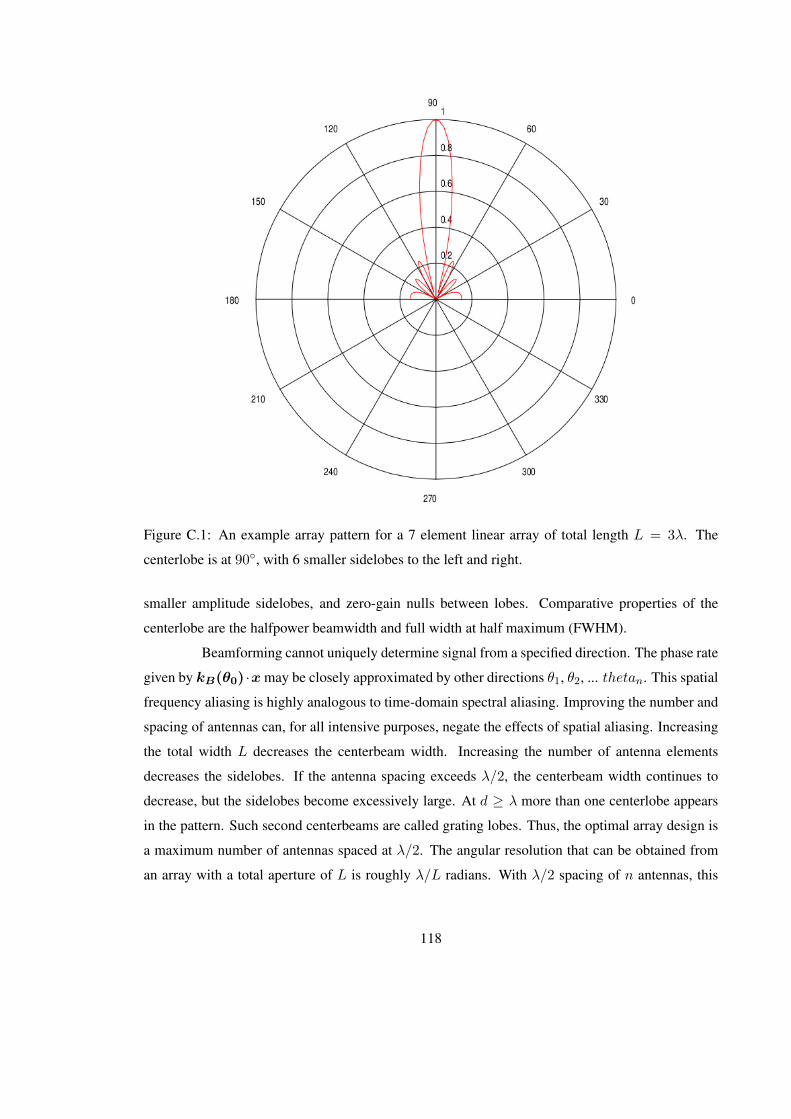
Figure C.1: An example array pattern for a 7 element linear array of total length L = 3λ. The
centerlobe is at 90, with 6 smaller sidelobes to the left and right.
smaller amplitude sidelobes, and zero-gain nulls between lobes. Comparative properties of the
centerlobe are the halfpower beamwidth and full width at half maximum (FWHM).
Beamforming cannot uniquely determine signal from a specified direction. The phase rate
given by kB(θ0) ·xmay be closely approximated by other directions θ1, θ2, ... thetan. This spatial
frequency aliasing is highly analogous to time-domain spectral aliasing. Improving the number and
spacing of antennas can, for all intensive purposes, negate the effects of spatial aliasing. Increasing
the total width L decreases the centerbeam width. Increasing the number of antenna elements
decreases the sidelobes. If the antenna spacing exceeds λ/2, the centerbeam width continues to
decrease, but the sidelobes become excessively large. At d ≥ λ more than one centerlobe appears
in the pattern. Such second centerbeams are called grating lobes. Thus, the optimal array design is
a maximum number of antennas spaced at λ/2. The angular resolution that can be obtained from
an array with a total aperture of L is roughly λ/L radians. With λ/2 spacing of n antennas, this
118
simplifies to an angular resolution of 2/n. The array pattern varies with steering angle. As the
radiation pattern is steered broadside to endfire, i.e. orthogonal to parallel with the array, the width
of the centerbeam becomes larger.
Applying only phase shifts to each antenna in C.0.32 corresponds to a boxcar filter in the
space domain and a sinc function convolution in the spatial frequency domain. Judicious use of
windowing functions can improve the array pattern. The sinc function has a FWHM of 1.21 df/2π
with a peak sidelobe of ' 22%. The Hanning window gives 2 df/2π with a peak sidelobe of
' 2.6%. Combining an amplitude windowing function with the beamsteering phase shift, i.e. a
complex weight, improves control over side lobe levels at the expensive of centerlobe width. The
complex array factor w(~k) acts as a transfer function:
wk = akeiθk (C.0.33)
where wk are the complex weights for each k antenna element, ak is the relative amplitude of the
weight, and θk is the phase shift of the weight. For uniformly spaced arrays, array factor design
methods are identical to the methods for designing FIR digital filters in signal processing. As well
as controlling the centerlobe width and sidelobe levels, the position of a null can be controlled.
A variety of errors can affect beamforming. It is important that the amplitude and phase
response of the antennas is well known and incorporated into the array factor. Antenna ground
planes, cables, buried conductors, fences, and ground conductivity all contribute to the array factor.
Land path propagation of the EM wave can have a varying response with direction. Much of the
array factor error can be corrected by careful calibration of the radar system.
119
Appendix D
Vector Correlation
The following is from a short paper on vector correlation [Hanson et al., 1992].
Consider the correlation between n pairs of two dimensional vectors, represented as com-
plex numbers zj and wj . Variance and covariance can be defined as:
σ2z =
1
n
n∑j=1
(zj − z)∗(zj − z) = σ2x + σ2
y (D.0.34)
σzw =1
n
n∑j=1
(zj − z)∗(wj −w) = (σxu + σyv) + i(σxv − σyu) (D.0.35)
where * indicates complex conjugate.
The variance of zj is the sum of the component variances while the covariance is a vector.
The real portion σxu + σyv is the sum of the covariances between corresponding components of the
variables. The imaginary portion σxv − σyu measures the ”twisting” of one vector’s components
into the opposite components of the other vector. Twisting implies a direction (from one vector into
another) so vector covariance contains the asymmetry σzw = σ∗wz not found in scalar covariance.
The vector correlation is defined as:
ρzw =σzwσzσw
(D.0.36)
which is analogous to scalar correlation. The squared magnitude of the correlation ρzwρ∗zw is
the proportion of the variance in wj explained by the regression equation. The magnitude of the
correlation is in the range zero to one and is unaffected by linear transformation of either zj orwj .
Consider the regression equation
120

wj = βzj + α+ εj (D.0.37)
with the complex regression coefficients β = b0 + ib1 and α = a0 + ia1. Fit error associated with
the jth observation is εj . A least-squares regression then requires that α and β minimize∑εjε∗j .
The regression coefficients are:
β = ρzwσwσz
(D.0.38)
and
α = w − βz (D.0.39)
Equation D.0.37 implies a transformation that involves translation, rotation, and scaling
of the vector zj . The intercept α defines a translation of coordinates. Rotation and scaling are
contained in β, in the magnitude and phase of β, respectively. The phase angle Θ of β can be
derived directly from the correlation:
tan Θ =ImρzwReρzw
=σxv − σyuσxu + σyv
(D.0.40)
These are useful quantities. The magnitude of β is a scaling factor that describes relative
magnitudes of vector components. The phase of β describes a consistent phase offset. Neither the
correlation magnitude nor the magnitude of β retain a sign. The phase Θ carries the information
analogous to sign in scalar correlation, but with more possibilities.
Equation D.0.34 can be modified to obtain a correlation that describes a reflectional rela-
tionship between two sets of vectors.
σz∗w =1
n
n∑j=1
(z∗j − z∗)∗(wj −w) = (σxu − σyv) + i(σxv + σyu) (D.0.41)
As with the rotation, reflectional correlation magnitude expresses goodness-of-fit, and the
magnitude of β is the scaling factor. The phase Θ of β indicates twice the axis of reflection - the
direction of the line about which variations in the paired observations are approximately symmetric.
Owing to the symmetry of the reflectional correlation, Θ keeps the same value regardless of whether
z or w is the independent vector.
Whether rotation or reflection is the better model can be determined by calculating the
rotation/reflection index:
121

ξ = σxuσyv − σxvσyu (D.0.42)
When ξ is positive, rotation is a better model, whereas if ξ is negative, reflection is bet-
ter. The physical interpretation of a reflectional relationship is somewhat confusing. Regardless,
it is a fundamentally different correlation estimate than rotational vector correlation. This is evi-
dent from the 4 independent terms in D.0.42, which boil down to∑z∗w vs.
∑zw. Thus the
rotation/reflection index D.0.42 should be included in any correlation analysis as a check on which
model is more appropriate.
122
Bibliography
M.L. Banner and I.R. Young. Modeling spectral dissipation in the evolution of wind waves. part i:
Assessment of existing model performance. J. Phys. Oceanogr., 24:1550–1571, 1993.
D.E. Barrick. The interaction of hf/vhf radio waves with the sea surface and its implications. In
AGARD Conference Proceedings, number 77 in Electromagnetics of the Sea, Sprinfield, VA.,
1970. Clearinghouse for Federal Scientific and Technical Information. accession no. AD716305.
D.E. Barrick. Theory of hf and vhf propagation across the rough sea, 1, the effective surface
impedance for a slightly rough highly conducting medium at grazing incidence. Radio Science,
6(5):517–526, 1971a.
D.E. Barrick. Theory of hf and vhf propagation across the rough sea, 2, application to hf and vhf
propagation above the sea. Radio Science, 6(5):527–533, 1971b.
D.E. Barrick. First-order theory and analysis of mf/hf/vhf scatter from the sea. IEEE Trans. Anten-
nas Propagat., AP-20:2–10, 1972.
D.E. Barrick. Extraction of wave parameters from measured hf radar sea-echo doppler spectra.
Radio Science, 12(3):415–424, 1977.
D.E. Barrick. Accuracy of parameter extraction from sample-averaged sea-echo doppler spectra.
IEEE Transactions on Antennas and Propagation, AP-28(1):1–11, 1980.
D.E. Barrick. Effects of shallow water on radar measurements. Codar report, CODAR Ocean
Sensors, January 2005a.
D.E. Barrick. Geometrical dilution of statistical accuracy (gdosa) in multi-static hf radar networks.
CODAR reference document, January 2005b.
D.E. Barrick and B.J. Lipa. The role of the gravity-wave dispersion relation in hf radar measure-
ments of the sea surface. Oceanic Engineering, IEEE Journal of, 11(2):289–292, 1986.
123

D.E. Barrick and B.L. Weber. On the nonlinear theory for gravity waves on the ocean’s surface. part
ii: Interpretation and applications. J. Phys. Oceanogr., 7(1):11–21, 1977.
D.E. Barrick, M.W. Evans, and B.L. Weber. Ocean surface currents mapped by radar. Science, 198:
138–144, 1977.
W.L. Bragg. The diffraction of short electromagnetic waves by a crystal. Proceedigns of the Cam-
bridge Philosophical Society, 17:43–57, 1913.
S.I. Caires. Comparative study of HF radar measurements and wave model hindcasts of waves in
shallow water. PhD thesis, University of Sheffield, September 2000.
C. Chavanne. Observations of the Impact of Mesoscale Currents on Internal Tide Propagation. PhD
thesis, University of Hawaii, USA, 2007.
C. Chavanne, I. Janekovic, P. Flament, P.M. Poulain, M. Kuzmic, and K.W. Gurgel. Tidal currents in
the northwestern adriatic: High-frequency radio observations and numerical model predictions.
J. Geophys. Res., 112:CO3S21, 1–18, 2007.
S.B. Colegrove. Project jindalee: from bare bones to operational othr. In The Record of the IEEE
2000 International Radar Conference, 2000, pages 825–830, Alexandria, VA, May 2000.
D.D. Crombie. Doppler spectrum of sea echo at 13-56 mc/s. Nature, 175:681–682, 1955.
D.D. Crombie. Spectral characteristics of hf ground wave signals backscattered from the sea. In
Electromagnetics of the Sea, number 77 in AGARD Conference Proceedings, 1970.
D.D Crombie. Resonant backscatter from the sea and its application to physical oceanography. In
IEEE International Conference Proceedings on Engineering in the Ocean Environment, pages
174–179, New York, 1972. IEEE.
V.E. Derr, editor. Remote Sensing of the Troposphere, chapter Remote Sensing of Sea State by
Radar, pages 12–1–12–46. U.S. National Oceanic and Atmospheric Administration; for sale by
the Supt. of Docs., U.S. Govt. Print. Off., Washington, 1972.
M.A. Donelan, Hamilton.J., and W.H. Hui. Directional spectra of wind-generated waves. Philo-
sophical Transactions of the Royal Society of London, 315:509–562, 1985.
H.H. Essen, K.W. Gurgel, and T. Schlick. Measurement of ocean wave height and direction by
means of hf radar: an empirical approach. Ocean Dynamics, 1999.
124

D.M. Fernandez, H.C Graber, J.D Paduan, and D.E. Barrick. Mapping wind direction with hf radar.
Oceanography, 10(2):93–95, 1997.
D.B. Gilhousen. A field evaluation of ndbc moored data buoy winds. J. Atmos. Oceanic Technol.,
4:94–104, 1987.
H.C. Graber, D.R. Thompson, and R.E. Carande. Ocean surface features and currents measured with
synthetic aperture radar interferometry and hf radar. J. Geophys. Res., 101(C11):25,813–25,832,
1996.
K.W. Gurgel and Y. Barbin. Suppressing radio frequency interference in hf radars. Sea Technology,
pages 39–42, March 2008.
K.W. Gurgel and H.H Essen. On the performance of a ship-borne current mapping hf radar. IEEE
Journal of Oceanic Engineering, 25(1):183–191, 2000.
K.W. Gurgel, G. Antonischki, H.H. Essen, and T. Schlick. Wellen radar (wera), a new ground-wave
based radar for ocean remote sensing. Coastal Engineering, 37:219–234, 1999a.
K.W. Gurgel, H.H. Essen, and S.P. Kingsley. Hf radars: Physical limitations and recent develop-
ments. Coastal Engineering, 37:201–218, 1999b.
K.W. Gurgel, H.H. Essen, and T. Schlick. An empirical method to derive ocean waves from second-
order bragg scattering: Prospects and limitations. IEEE Journal of Oceanic Engineering, 31(4):
804–811, 2006.
B. Hanson, K. Klink, K. Matsuura, S.M. Robeson, and C.J. Willmott. Vector correlation: Review,
exposition, and geographic application. Annals of the Association of American Geographers, 82
(1):103–116, 1992.
J. Harlan and T. Georges. An empirical relation between ocean-surface wind direction and the bragg
line ratio of hf radar sea echo spectra. J. Geophys. Res., 99:7971–7978, 1994.
K. Hasselmann. Feynman diagrams and interaction rules of wave-wave scattering processes. Re-
views of Geophysics, 4(1):1–32, 1966.
K. Hasselmann. Determination of ocean-wave spectra from doppler radio return from the sea sur-
face. Nature, 299:16–17, 1971.
125
M.L. Heron and S.F. Heron. Cumulative probability noise analysis in geophysical spectral records.
Internaional Journal of Remote Sensing, 22(13):2537–2544, 2001.
M.L. Heron, P.E. Dexter, and B.T. McGann. Parameters of the air-sea interface by high-frequency
ground-wave doppler radar. Aust. J. Mar. Freshwater Res., 36:655–670, 1985.
M.L. Heron, H.C. Graber, and S.F. Heron. Validation of routine waveheight measurements on hf
ocean radars. In OCEANS 1998 Conference Proceedings, volume 1, pages 454–458, 1998.
Y. Jun, W. Biyang, and W. Shicai. Method to suppress radio-frequency interference in hf radars.
Electronics Letters, 40(2):145–146, 2004.
K.E. Kenyon. Stokes drift for random gravity waves. J. Geophys. Res., 74(28):6991–6994, 1969.
M. Kline, editor. Theory of Electromagnetic Waves, chapter Reflection of electromagnetic waves
from slightly rough surfaces, pages 351–378. Interscience and Dover, New York, 1951.
P.M. Kosro, J.A. Barth, and P.T. Strub. The coastal jet: Observations of surface currents over the
oregon continental shelf from hf radar. Oceanography, 10(2):53–56, 1997.
P.K. Kundu, I.M. Cohen, and H.H. Hu. Fluid Mechanics, chapter 7, pages 238–240. Elsevier
Academic Press, 3rd edition, 2004.
K. Laws, J.D. Paduan, and D.M. Fernandez. Effect of stokes drift on hf radar measurements. In H.C.
Graber and J.D. Paduan, editors, Radiowave Oceanography: The First International Workshop,
pages 51–57, April 2001.
B.J. Lipa and D.E. Barrick. Least-squares method for the extraction of surface currents from codar
crossed-loop data: Application at arsloe. IEEE J. Ocean Eng., 8:226–253, 1983.
B.J. Lipa and B. Nyden. Directional wave information from the seasonde. IEEE Journal of Oceanic
Engineeering, 30(1):221–231, 2005.
A.E Long and D.B. Trizna. Mapping of north atlantic winds by hf radar sea backscatter interpreta-
tion. IEEE Trans. Antennas Propag., AP-21:680–685, 1973.
M.S. Longuet-Higgins and O.M. Phillips. Phase velocity effects in tertiary wave interactions. Jour-
nal of Fluid Mechanics, 12:333–336, 1962.
126

M.S. Longuet-Higgins, D.E. Cartwright, and N.D. Smith. Ocean Wave Spectra, chapter Observa-
tions of the Directional Spectrum of Sea Waves using Motions of a Floating Buoy. Prentice-Hall,
Englewood Cliffs, NJ, 1963.
A. Lygre and H.E. Krogstad. Maximum entropy estimation of the directional distribution in ocean
wave spectra. J. Phys. Oceanogr., 16(12):2052–2060, 1986.
J.W. Maresca and T. Georges. Measuring rms wave height and the scalar ocean wave spectrum with
hf skywave radar. J. Geophys. Res., 85(C5):2759–2771, 1980.
D. Masson. Observations of the response of sea waves to veering winds. J. Phys. Oceanogr., 20:
18876–1885, 1990.
K.J. Molnar, W. Lin, and M. O’Donnell. Beamforming and aberration correction in hf radar. In
Record of the IEEE 1990 International Radar Conference, pages 90–95, 1990.
W.A. Nierenberg and W.H. Munk. Sea spectra and radar scattering. In Working Paper, 1969 Jason
Summer Study. ””, Boulder, CO, 1969.
H. Nyquist. Thermal agitation of electric charge in conductors. Physical Review, 32(1):110–113,
1928.
A.M Peterson, C.C. Teague, and G.L. Tyler. Bistatic-radar observation of long-period, directional
ocean-wave spectra with loran a. Science, 170(3954):158–161, 1970.
O.M. Phillips. The equilibrium range in the spectrum of wind-generated ocean waves. J. Marine
Res., 16:231–245, 1958.
O.M. Phillips. Dynamics of the Upper Ocean. Cambridge University Press, London, 1966.
W.J. Pierson Jr. Examples of, reasons for, and consequences of the poor quality of wind data from
ships for the marine boundary layer: Implications for remote sensing. J. Geophys. Res., 95:
13,313–13,340, 1990.
A.M. Ponsford, R.M. Dizaji, and R. McKerracher. Hf surface wave radar operation in adverse
conditions. In Proceedings of the International Conference on Radar, pages 593–598, 2003.
D. Prandle. The fine-structure of nearshore tidal and residual circulations revealed by h.f. radar
surface current measurements. J. Phys. Oceanogr., 17(2):231–245, 1987.
127
D. Prandle and D.K. Ryder. Measurement of surface currents in liverpool bay by high frequency
radar. Nature, 315:128–131, 1985.
D. Prandle and D.K. Ryder. Comparison of observed and modeled nearshore velocities. Continental
Shelf Research, 9(12):1029–1104, 1989.
G.T. Ruck, D.E. Barrick, W.D. Stuart, and C.K. Krichbaum. Radar Cross Section Handbook, vol-
ume 1. Plenum Press, New York, 1970. pg. 53.
J.A. Saxton, editor. Advances in Radio Research, volume 1, chapter Electromagnetic surface waves,
pages 157–217. Academic, New York, 1964.
R.O. Schmidt. Multiple emitter location and signal parameter estimation. IEEE Trans. Antennas
Propag., 34:276–280, 1986.
L.K. Shay. Internal wave-driven surface currents from hf radar. Oceanography, 10(2):60–63, 1997.
L.K. Shay, H.C. Graber, D.B. Ross, and R.D. Chapman. Mesoscale ocean surface current structure
detected by high-frequency radar. Journal of Atmospheric and Oceanic Technology, 12(4):881–
900, 1995.
E.D. Shearman and L.R. Wyatt. Dekametric radar for surveillance of sea-state and oceanic winds.
The Journal of Navigation, 35:397–40, 1982.
V.I. Shrira, D.V. Ivonin, P. Broche, and J.C. de Maistre. On remote sensing of vertical shear of
ocean surface currents by means of a single-frequency vhf radar. Geophysical Research Letters,
28(20):3955–3958, 2001.
R.H. Stewart and J.R. Barnum. Radio measurements of oceanic winds at long ranges: An evaluation.
J. Phys. Oceanogr., 10:128–143, 1975.
R.H. Stewart and J.W. Joy. Hf radio measurements of ocean surface currents. Deep Sea Research,
21:1039–1049, 1974.
G.G. Stokes. On the theory of oscillatory waves. Transactions of the Cambridge Philosophical
Society, 8:441–445, 1847.
C.C. Teague. High-Frequency Resonant Scattering Techniques for Observation of Directional
Ocean-Wave Spectra. PhD thesis, Stanford University, Stanford, California, 1971.
128

C.C. Teague, J.F. Vesecky, and D.M. Fernandez. Hf radar instruments, past to present. Oceanogra-
phy, 10(2):40–44, 1997.
G.L. Tyler, W.E. Faulkerson, A.M. Peterson, and C.C. Teague. Second-order scattering from the
sea: Ten-meter radar observations of the doppler continuum. Science, 177(4046):349–351, 1972.
G.P. van Vledder and L.H. Holthuijsen. The directional response of ocean waves to turning winds.
J. Phys. Oceanogr., 23(2):177–192, 1993.
J.F. Vesecky, J. Drake, C.C. Teague, F.L. Ludwig, K. Davidson, and J. Paduan. Measurement of
wind speed and direction using multifrequency hf radar. In Geoscience and Remote Sensing
Symposium, IGARSS, pages 1899–1901. IEEE International, 2002.
H. von Storch and F.W. Zwiers. Statistical analysis in climate research. Cambridge University
Press, Cambridge, 1999.
B.L. Weber and D.E. Barrick. On the nonlinear theory for gravity waves on the ocean’s surface. part
i: Derivations. J. Phys. Oceanogr., 7(1):3–10, 1977.
L.R Wyatt. The ocean wave directional spectrum. Oceanography, 10:85–89, 1997.
L.R. Wyatt. Hf radar wind measurement - present capabilities and future prospects. In H.C. Graber
and J.D. Paduan, editors, Radiowave Oceanography: The First International Workshop, pages
82–87, April 2001.
L.R. Wyatt and J.J. Green. The availability and accuracy of hf radar wave measurements. In 2002
IEEE International Geoscience and Remote Sensing Symposium, pages 515–517, 2002.
L.R. Wyatt, S.P. Thompson, and R.R. Burton. Evaluation of high frequency radar measurement.
Coastal Engineering, 37:259–282, 1999.
L.R. Wyatt, J.J. Green, K.W. Gurgel, J.C. ”Nieto Borge”, K. Reichert, K. Hessner, H. Gunther,
W. Rosenthal, O. Saetra, and M. Reistad. Validation and intercomparisons of wave measurements
and models during the eurorose experiments. Coastal Engineering, 48:1–28, 2003.
L.R Wyatt, G. Liakhovetski, H.C. Graber, and B.K. Haus. Factors affecting the accuracy of showex
hf radar wave measurements. Journal of Atmospheric and Oceanic Technology, 22:847–859,
2005.
129

L.R Wyatt, J.J. Green, A. Middleditch, M.D. Moorhead, J. Howarth, M. Holt, and S. Keogh. Oper-
ational wave, current, and wind measurements with the pisces hf radar. IEEE Journal of Oceanic
Engineering, 31(4):819–834, 2006.
130