Radar presentation plan 1. General radar: Chap1.doc 2. Lecture03.ppt (general) 3. xprinfo 4. radarinfo.doc 5. radareq.doc 6. logarith.doc 7. radar-eq-notes.ppt 8. 88d-minZ.xls 9. noise.doc 10. note on reflectivity measurements.doc 11. Homework: z-calc-prob.doc radareq-prob.doc 12. Calibration - Atlas paper 13. Radar sampling  

Ground-Based Remote Sensing Part I: Active Remote Sensors Chap. 1: Introduction to radar 1/26/10

Active Remote Sensor: Transmits radiation of specific frequency (or frequency interval) and receives it via reflection or backscattering from a point target or distribution of targets (e.g., raindrops) 1. Introduction to radar Good overview: www.fas.org/man/dod-101/navy/docs/swos/cmd/fun12/12-1/sld006.htm 1.1 Background Definitions: RADAR -- Radio Detection and Ranging Range of wavelengths: 1 mm < λ < 10 m Specific radar bands: refer to handout sheet Doppler (coherent) radar – ability to measure change in phase of transmitted signal Incoherent radar – phase change not measured, only magnitude of backscattered signal is measured Radar strengths – ability to detect clouds, precipitation, and refractive index variations Radar limiations – crude spatial resolution, spectral limitations, side lobe contamination, ambiguous signals 1.2 Radar History (Rinehart, pp. 1-4) Radar Meteorological radar Doppler radar Polarimetric radars 1.3 Radar hardware overview 1.3.1 Radar types Pulsed – radiation emitted in short pulses (~1 µs) at some pulse repetition frequency (PRF) Continuous wave (CW) – radiation emitted continuously Bistatic – two antennas, one transmits and one receives Monostratic – one antenna (transmits and receives), more common 1.3.2 Radar components Transmitter Source of EM radiation; generates signal at specific radio frequency (RF)

Transmitter types Magnetron – an oscillator tube with resonant cavities (Fig. 6.2, Skolnik) Developed in 1939 Small, relatively cheap Can transmit signals with peak energy of ~500 kW coaxial magnetron – improved power, frequency stability, efficiency and life (Fig. 6.3, Skolnik) Fig. 2.2 in Rinehart Example: HSV WSR-74C radar (coaxial magnetron) Klystron – power amplifier fed by a RF oscillator (true amplifier) Also contain cavities (Fig. 6.9, Skolnik)

Larger and more power, peak transmit power up to 2 MW Good waveform, purer (very stable) transmit frequency Also termed MOPA – Master Oscillator Power Amplifier Example: WSR-88D radar

Ground-Based Remote Sensing Part I: Active Remote Sensors Chap. 1: Introduction to radar 1/26/10

Solid state transmitter Much lower power (<1000 W ?) Can be used in clusters to produce greater peak power Example: 915 MHz Doppler radar profiler (UAH MIPS, ~500 W)

Modulator Switches transmitter on and off Controls the waveform of the transmitted pulse Stores energy between pulses Master cloud or timer (or computer) Controls pulse repetition frequency (PRF) and pulse duration (τ) PRF – number of pulses per sec PRF ~ 103 s-1 Pulse Repetition Period (PRP) = 1/PRF (~1 ms) PRF determines the maximum unambiguous range (Rmax) – more details later Rmax = c/(2⋅PRF) For PRF = 1000 s-1, Rmax = 150 km Recovery time of transmitter defines minimum range (Rmin), 0.1-2 km Transmitted signal is ideally rectangular, but in reality more Gaussian in shape (Fig. from D&Z) Pulse length – h = cτ/2 (for τ = 1 µs, h = 150 m) Waveguide – a hollow metal conductor with rectangular cross section (Fig. 2.3 Rinehart) Most efficient way of getting transmitted pulse (signal) to the antenna Wires and coaxial cable experience more loss Coaxial cable is used effectively in lower frequency radars (e.g., 915 MHz profiler) Longer dimension is in the direction of the E field, the shorter in the direction of the H field Waveguide dimension is λ/2 Pieces: straight sections with flange and choke joints, curved sections, and rotary joints Antennna Antenna “system” consists of feedhorn and dish reflector Wave guide carries signal from transmitter to feedhorn Directs the signal into a narrow beam, typically 0.5-2.0° Dish diameters 0.3-9 m; define the beamwidth for give λ; larger λ requires larger dish Dish provides directional capability and gain (g or G) g = Pmeas/ Pisotropic

(maximum directional gain in linear units) G = 10 log10(Pmeas/Pisotropic) (units in dB) Isotropic power density Pisotropic given by Pisotropic = Pt/(4πr2) Beamwidth and gain are related G = π2k2/θφ k-shape factor (1), θ,φ are horizontal and vertical beamwidth G = π2/θ2 for circular dish with parabolic cross section For θ = 1°, G = π2 / (1° x π/180°) = 32400 = 45.1 dB Antenna types (Fig from Battan, last time) – most common is circular with parabolic cross section Antenna beam patterns are irregular and “messy” Figs. 2.2, 2.3 and 2.4 of Rinehart Main lobe, side lobes, back lobes First side lobes typically –20 to –30 dB below peak Beam width is defined by the angular distance between half power points (-3 dB down) Approximate formula: θ1 = 1.27λ/D (radian) Main lobe shape g = g0exp[-(θ/θ1)2] for a Gaussian beam (good approximation) or in log scale, G = G0 –4.343(θ/θ1)2 Side lobe power ~1% of power in main lobe Theoretical antenna beam illumination pattern (from Eq. 3.2a of D&Z)

Ground-Based Remote Sensing Part I: Active Remote Sensors Chap. 1: Introduction to radar 1/26/10

where θ is the angular distance from the beam axis and J2 is the Bessel function of the 2nd order. [Note: refer to http://en.wikipedia.org/wiki/Bessel_function

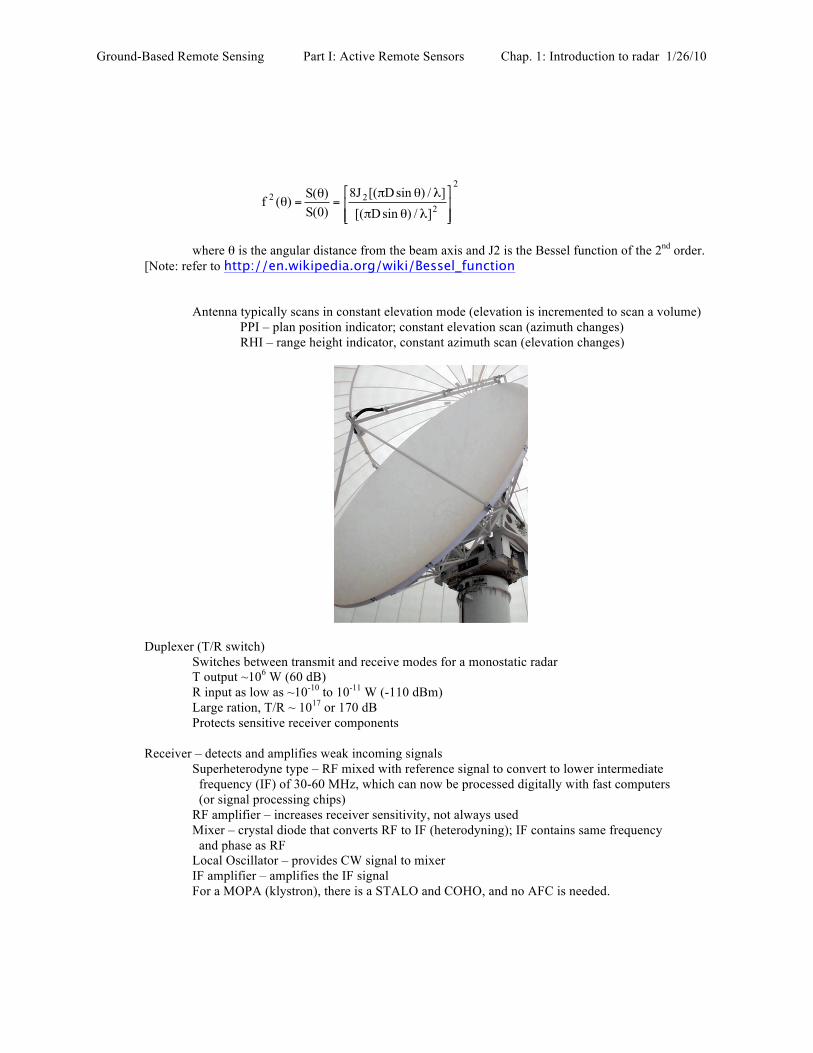
Antenna typically scans in constant elevation mode (elevation is incremented to scan a volume) PPI – plan position indicator; constant elevation scan (azimuth changes) RHI – range height indicator, constant azimuth scan (elevation changes)

Duplexer (T/R switch) Switches between transmit and receive modes for a monostatic radar T output ~106 W (60 dB) R input as low as ~10-10 to 10-11 W (-110 dBm) Large ration, T/R ~ 1017 or 170 dB Protects sensitive receiver components Receiver – detects and amplifies weak incoming signals Superheterodyne type – RF mixed with reference signal to convert to lower intermediate

frequency (IF) of 30-60 MHz, which can now be processed digitally with fast computers (or signal processing chips) RF amplifier – increases receiver sensitivity, not always used Mixer – crystal diode that converts RF to IF (heterodyning); IF contains same frequency and phase as RF Local Oscillator – provides CW signal to mixer IF amplifier – amplifies the IF signal For a MOPA (klystron), there is a STALO and COHO, and no AFC is needed.

2

222

]/)sinD[(]/)sinD[(J8

)0(S)(S)(f

!!"

#

$$%

&

λθπ

λθπ=

θ=θ

Ground-Based Remote Sensing Part I: Active Remote Sensors Chap. 1: Introduction to radar 1/26/10

Display A-scope PPI RHI

Aspects of the transmitted signal and received signal – refer to handouts from Rauber notes

1.4 Example of radar systems Preliminaries Monostatic vs. bistatic CW vs. pulsed Coherent (Doppler) vs incoherent Radars used in aviation ARSR - enroute surveillance radars (L band) ASR-9 – new Airport Surveillance Radar (S-band) that has a Doppler weather channel to monitor flow and

boundaries. HSV received one of the first ASR-9 radars. TDWR – terminal Doppler Weather Radar (C band, 0.5° beamwidth), located at major airports Aircraft radars – X-band (I think), located in nose section of aircraft); monitor weather ahead of aircraft

Weather radars Precipitation radars: X- C- and S-band WSR-88D is the NWS network S-band radar; specs in table below X and C-band will experience attenuation in rain (more on this later) Cloud radars (research): K band (λ = 3 mm and 8 mm are most common) Short wavelength is needed to detect small cloud particles (as demonstrated by radar eq.) Wind profiling radars: UHF and VHF (915, 405 and 50 MHz) Detect motions in clear air via scattering from refractive index irregularities (Bragg scatter) Radar specifications (See Rinehart, Appendix D) Table: WSR-88D specifications (taken from D&Z) Antenna subsystem Radome Type Fiberglass skin foam sandwich Diameter 11.89 m RF loss (two way) 0.3 dB Pedestal Type elevation over azimuth Azimuth Elevation Scanning rate 30° s-1 30° s-1

Acceleration 15° s-2 15° s-2 Mechanical limits -1° to 60° Reflector Type Paraboloid of revolution Polarization Linear horizontal Diameter 8.54 m Gain 44.5 dB Beamwidth 0.95° First sidelobe level -26 dB (with radome)

Ground-Based Remote Sensing Part I: Active Remote Sensors Chap. 1: Introduction to radar 1/26/10

Transmitter and Receiver subsystem Transmitter Type MOPA (klystron) Frequency 2700-3000 MHz Wavelength 10.7 cm Pulse power (peak) 1 MW Pulse duration 1.57 and 4.57 µs RF duty cycle 0.002 maximum PRFs Short pulse 320-1300 Hz (total of 8 selectable in this range) Long pulse 320 and 450 Hz Receiver Type Linear Dynamic range 93 dB Intermediate Frequency 57.6 MHz System noise power -113 dBm Filter Short pulse analog filter: bandwidth (3 dB): 0.63 MHz Bandwidth (6 dB): 0.80 MHz Long pulse Additional digital filtering; 3 samples

(spaced 0.25 km) of I and Q are averaged. Output samples are space at 0.5 km intervals.

Radar constant: 58.4 System performance: minimum reflectivity factor of –20.7 dBZ at 50 km Problem: Find (web search) radar specifications for the following three research radars and compare with the WSR-88D radar specifications a) CHILL radar b) NCAR S-Pol radar (S-band) c) Doppler on Wheels (DOW) X-band radar (Center for Severe Storms Research) d) A K- or W-band cloud radar (NOAA ETL) Radar systems Block diagram for a simple radar (From Rinehart, Fig. 2.1)

Ground-Based Remote Sensing Part I: Active Remote Sensors Chap. 1: Introduction to radar 1/26/10

Presentations: http://www.fas.org/man/dod-101/navy/docs/swos/cmd/fun12/12-1/sld001.htm http://apollo.lsc.vsc.edu/classes/remote/lecture_notes/radar/doppler/index.html www.owlnet.rice.edu/~nava201/presentations/Lecture03.ppt

Radar Principles &

Systems

With your facilitator, LT Mazat

I. Learning Objectives

A. The student will comprehend the basic operation of a simple pulse radar system. B. The student will know the following terms: pulse width, pulse repetition frequency, carrier frequency, peak power, average power, and duty cycle.

C. The student will know the block diagram of a simple pulse radar system and will comprehend the major components of that system.

D. The student will comprehend the basic operation of a simple continuous wave radar system.

E. The student will comprehend the concept of doppler frequency shift.

F. The student will know the block diagram of a simple continuous wave radar system and will comprehend the major components of that system, including amplifiers, power amplifiers, oscillators, and waveguides.

G. The student will comprehend the use of filters in a continuous wave radar system.

H. The student will know the fundamental means of imparting information to radio waves and will comprehend the uses, advantages, and disadvantages of the various means.

I. The student will comprehend the function and characteristics of radar/radio antennas and beam formation.

J. The student will comprehend the factors that affect radar performance.

K. The student will comprehend frequency modulated CW as a means of range determination.

L. The student will comprehend the basic principles of operation of pulse doppler radar and MTI systems.

Two Basic Radar Types

  Pulse Transmission

  Continuous Wave

Pulse Transmission

Range vs. Power/PW/PRF

• Minimum Range: If still transmitting when return received RETURN NOT SEEN.

• Max Range: PRFPWPRTPW

PeakPowererAveragePow *==

As min Rh max Rh

PW

PRF

 2. Pulse repetition frequency (PRF)  a. Pulses per second  b. Relation to pulse repetition time (PRT)   c. Effects of varying PRF

  (1) Maximum range   (2) Accuracy

 3. Peak power  a. Maximum signal power of any pulse  b. Affects maximum range of radar

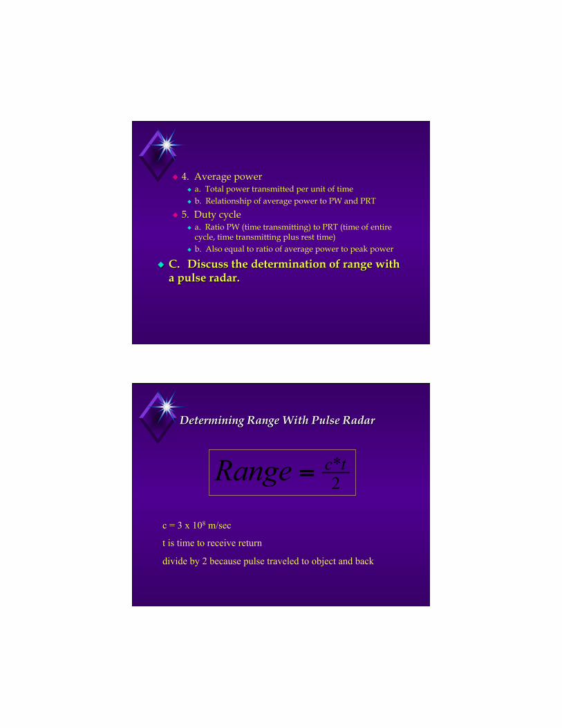
  4. Average power   a. Total power transmitted per unit of time   b. Relationship of average power to PW and PRT

  5. Duty cycle   a. Ratio PW (time transmitting) to PRT (time of entire

cycle, time transmitting plus rest time)   b. Also equal to ratio of average power to peak power

  C. Discuss the determination of range with a pulse radar.

Determining Range With Pulse Radar

2*tcRange =

c = 3 x 108 m/sec

t is time to receive return

divide by 2 because pulse traveled to object and back

Pulse Transmission   Pulse Width (PW)

  Length or duration of a given pulse   Pulse Repetition Time (PRT=1/PRF)

  PRT is time from beginning of one pulse to the beginning of the next

  PRF is frequency at which consecutive pulses are transmitted.

  PW can determine the radar’s minimum detection range; PW can determine the radar’s maximum detection range.

  PRF can determine the radar’s maximum detection range.

  D. Describe the components of a pulse radar system.   1. Synchronizer   2. Transmitter   3. Antenna   4. Duplexer   5. Receiver   6. Display unit   7. Power supply

Pulse Radar Block Diagram

Power

Supply

Synchronizer Transmitter

Display

Duplexer

(Switching Unit)

Receiver

Antenna

Antenna Bearing or Elevation

Video

Echo

ATR RF

TR

Continuous Wave Radar   Employs continual

RADAR transmission

  Separate transmit and receive antennas

  Relies on the “DOPPLER SHIFT”

Doppler Frequency Shifts

Motion Away: Echo Frequency Decreases

Motion Towards: Echo Frequency Increases

Continuous Wave Radar Components

Discriminator AMP Mixer

CW RF Oscillator

Indicator

OUT

IN

Transmitter Antenna

Antenna

Pulse Vs. Continuous Wave

Pulse Echo   Single Antenna   Gives Range,

usually Alt. as well   Susceptible To

Jamming   Physical Range

Determined By PW and PRF.

Continuous Wave   Requires 2 Antennae   Range or Alt. Info   High SNR   More Difficult to Jam

But Easily Deceived   Amp can be tuned to

look for expected frequencies

RADAR Wave Modulation

 Amplitude Modulation –  Vary the amplitude of the carrier sine wave

 Frequency Modulation –  Vary the frequency of the carrier sine wave

 Pulse-Amplitude Modulation –  Vary the amplitude of the pulses

 Pulse-Frequency Modulation –  Vary the Frequency at which the pulses occur

Modulation

Amplitude modulation

Freq. mod.

Pulse-amplitude modulation

Pulse frequency modulation

Antennae

 Two Basic Purposes:

 Radiates RF Energy

 Provides Beam Forming and Focus

 Must Be 1/2 of the Wave Length for the maximum wave length employed

 Wide Beam pattern for Search, Narrow for Track

Beamwidth Vs. Accuracy

Beamwidth vs Accuracy

Ship A Ship B

Azimuth Angular Measurement

Azimuth Angular MeasurementRelative Bearing = Angle from ship’s heading.True Bearing = Ship’s Heading + Relative Bearing

NShip’s Heading Angle

Target Angle

Determining Altitude

Determining Altitude

Slant Range

Altitude

Angle of Elevation

Altitude = slant range x sin0 elevation

Concentrating Radar Energy Through Beam Formation

 Linear Arrays   Uses the Principle of wave summation

(constructive interference) in a special direction and wave cancellation (destructive interference) in other directions.

  Made up of two or more simple half-wave antennas.

 Quasi-optical   Uses reflectors and “lenses” to shape the beam.

Basic Dipole Antenna and Beam Forming Half-Wave Dipole Antenna

Basic Beam Formed

Wave Shaping Linear Array

Beam Forming

Side

Bottom

Types of Linear Arrays

Broadside Endfire Array

Wave Shaping Linear Array Parasitic Element

Reflector Shape

 Paraboloid - Conical Scan used for fire control - can be CW or Pulse

 Orange Peel Paraboliod - Usually CW and primarily for fire control

 Parabolic Cylinder - Wide search beam - generally larger and used for long-range search applications - Pulse

Wave Shaping -Quasi-Optical Systems

Reflectors Lenses

Wave Guides   Used as a medium for

high energy shielding.   Uses A Magnetic Field

to keep the energy centered in the wave guide.

  Filled with an inert gas to prevent arcing due to high voltages within the waveguide.

Questions?

Please read Ch 9.

Radar Principles and Systems Part II

Factors That Affect Radar Performance

  Signal Reception   Receiver Bandwidth   Pulse Shape   Power Relation   Beam Width   Pulse Repetition

Frequency   Antenna Gain   Radar Cross Section of

Target

  Signal-to-noise ratio   Receiver Sensitivity   Pulse Compression   Scan Rate

  Mechanical   Electronic

  Carrier Frequency   Antenna aperture

Radar Receiver Performance Factors

  Signal Reception   Signal-to-Noise Ratio   Receiver Bandwidth   Receiver Sensitivity

Signal Reception

• Only a minute portion of the RF is reflected off the target.

• Only a fraction of that returns to the antenna.

• The weaker the signal that the receiver can process, the greater the effective range .

Signal-to-Noise Ratio

  Measured in dB!!!!!   Ability to recognize target in random noise.

  Noise is always present.   At some range, noise is greater that target’s

return.

  Noise sets the absolute lower limit of the unit’s sensitivity.

  Threshold level used to remove excess noise.

Receiver Bandwidth

  Is the frequency range the receiver can process.

  Receiver must process many frequencies   Pulse are generated by summation of sine waves

of various frequencies.   Frequency shifts occur from Doppler Effects.

  Reducing the bandwidth   Increases the signal-to-noise ratio(good)   Distorts the transmitted pulse(bad)

Receiver Sensitivity

 Smallest return signal that is discernible against the noise background.  Milliwatts range.

 An important factor in determining the unit’s maximum range.

Pulse Effects on Radar Performance

 Pulse Shape  Pulse Width  Pulse Compression  Pulse Power

Pulse Shape

 Determines range accuracy and minimum and maximum range.

  Ideally we want a pulse with vertical leading and trailing edges.  Very clear signal – easily discerned when

listening for the echo.

Pulse Width

 Determines the range resolution.  Determines the minimum detection

range.  Can also determine the maximum

range of radar.  The narrower the pulse, the better the

range resolution.

Pulse Compression

  Increases frequency of the wave within the pulse.

 Allows for good range resolution while packing enough power to provide a large maximum range.

Pulse Power

 The “Ummph” to get the signal out a long way.

 High peak power is desirable to achieve maximum ranges.

 Low power means smaller and more compact radar units and less power required to operate.

Other Factors Affecting Performance

  Scan Rate and Beam Width   Narrow beam require slower antenna rotation rate.

  Pulse Repetition Frequency   Determines radars maximum range(tactical factor).

  Carrier Frequency   Determines antenna size, beam directivity and target size.

  Radar Cross Section (What the radar can see(reflect))   Function of target size, shape, material, angle and carrier

frequency.

Summary of Factors and Compromises

Summary of Factors and Compromises

Pulse Shape Sharp a rise as possible Better range accuracy Require infinite bandwidth, more complex Tall as possible More power /longer range Requires larger equipment/more power

Pulse Width Short as possible Closer minimum range Reduces maximum range More accurate range

Pulse Repetition Freq. Short Better range accuracy Reduces maximum range Better angular resolution

Better detection probability Pulse Compression Uses technique Greater range More complex circuitry

Shorter minimum range Power More Greater maximum range Requires larger equipment & power Beam Width Narrow Greater angular accuracy Slow antenna rate, Detection time Carrier Frequency High Greater target resolution Reduces maximum range

Detects smaller targets Smaller equipment

Receiver Sensitivity High Maximizes detection range More complex equipment Receiver Bandwidth Narrow Better signal-to-noise ratio Distorts pulse shape

Factor Desired Why Trade-off Required

Types of Radar Output Displays

  A Scan   Used for gunfire control   Accurate Range information

  B Scan   Used for airborne fire control   Range and Bearing, forward looking

  E Scan   Used for Altitude

  PPI   Used for surface search and navigation

Specific Types of Radar

  Frequency Modulated CW Radar   Use for radar altimeters and missile guidance.

  Pulse Doppler   Carrier wave frequency within pulse is compared with a

reference signal to detect moving targets.

  Moving Target Indicator (MTI) System   Signals compared with previous return to enhance moving

targets. (search radars)

  Frequency Agile Systems   Difficult to jam.

Specific Types of Radar

 SAR / ISAR  Phased Array - Aegis

 Essentially 360° Coverage  Phase shift and frequency shift allow the

planar array to “steer” the beam.  Also allows for high / low power output

depending on requirements.

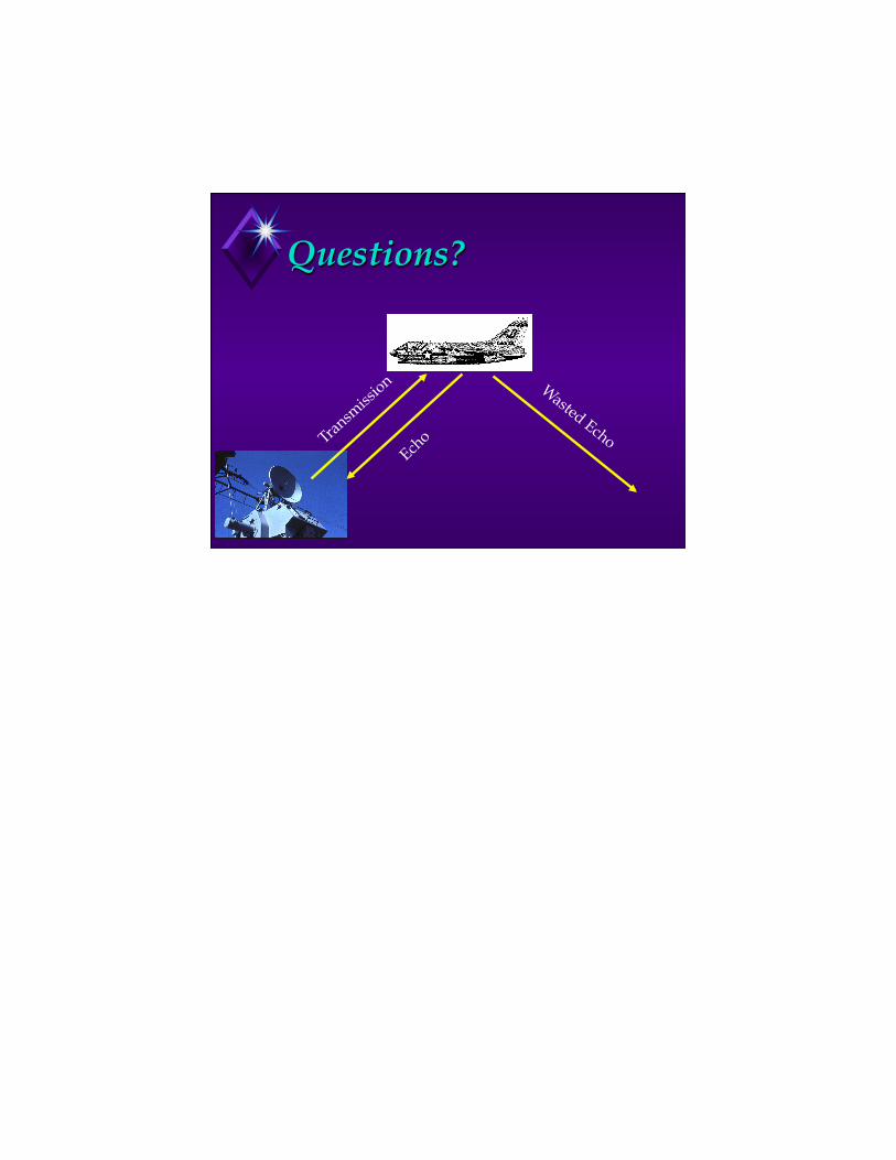
Questions?

Wasted Echo

Specifications for the XPR

1. X-Band magnetron transmitter peak power:

25 kW peak (nominal).

2. Polarization:

Horizontal (it’s an Andrew HP6-102-P3A microwave antenna, single

polarization).

3. Pulse duration range:

User can select between 1.0, 0.38, or 0.19 µs.

4. Range to first gate:

The Gamic system starts taking data right after sending the transmit pulse, so

the first sample comes from the 0 to 50 m range (assuming 50 m range gate

spacing). Second gate would come from the 50 to 100 m range, and so on. 5. Range gate spacing (selectable) values:

Set to 50 m by default. It could be set to larger values in 50 m increments,

e.g., 100 m, 150 m, etc.

6. Pulse repetition frequency (range):

Set to 500 Hz (1.0 µs PW), 1,250 Hz (0.38 µs PW), and 2,000 Hz (0.19 µs

PW). 7. Antenna diameter:

1.8 m.

8. Beam width:

1.2 degrees according to the Andrew HP6-102-P3A specifications, but we

have redesigned the antenna feed. Antenna pattern calculations are currently

being carried out. 9. Transmit frequency:

9.410 GHz. 10. Noise floor (dBm):

We will make measurements later on.

11. Number of range gates:

number of range gates = (maximum range) / (range spacing)

= 10 km / 50 m = 200

4,096 is the maximum number of range gates. If the number exceeds 4,096

the Gamic software will automatically adjust the maximum range (or slant

range as it is called in the Gamic software). 12. Number of points in the Doppler spectrum:

Set to 50. Doppler spectrum is calculated using the DFT algorithm. User can

change this value along with the data processing algorithm (DFT, FFT, or

PPP). 13. Recorded parameters:

Corrected and uncorrected reflectivity.

Mean velocity.

Spectral width.

In-phase and quadrature (I and Q ) time series.

If I and Q and processed, Doppler spectra can be calculated. 14. Dwell times (minimum, maximum):

I usually associate dwell times with the time the antenna is pointing in one

direction and this antenna is fixed in the vertical direction. Instead I will

calculate the times taken to get one estimate of the velocity:

dwell time = (number of time samples) / PRF (maximum samples is 255)

PRF = 500 Hz : dwell time = 0.51 s (samples = 255)

PRF = 1,250 Hz : dwell time = 0.204 s (samples = 255)

PRF = 2,000 Hz : dwell time = 0.1275 s (samples = 255)

RADAR EQUATION DEVELOPMENT 1/17/12

24 rP

P tisotropic π

= Power density from isotropic radiation ~ r-2

GPPantenna

isotropic=

!

"#

$

%&10 10log Definition of antenna gain (the ability to focus the radiation

along a narrow beam)

PP GAr

tσ

σ

π=4 2 Amount of power intercepted by a target with area Aσ

( )P P

Ar

P GA Arr

e t e= =σσ

π π4 42 2 4 Power returned to radar assuming isotropic re-radiation

Ae is the effective cross section of antenna Aρ is the cross sectional area; ρ is antenna efficiency Ae = ρAρ

A G GA

e = =λπ

π

λρ

2

2483

; From antenna theory (Silva, 1951 and others -- old)

→ =A Ae

23 ρ

( )P

P G Ar

P A Arr

t t= ≅

2 2

3 4

2

2 44 9λ

π πλσ ρ σ This assumes isotropic re-radiation of the scatterer, which

is never the case for meteorological targets. Define: backscattering cross section (σ): area intercepting that amount of power which, if scattered isotropically, would return to the receiver the amount actually received.

σ π σπ

P r Sr SPii

= → =442

2

Pi is incident power, S is backscattered power at antenna

( )PP G

rrt i=2 2

3 44λ σ

π σi is the bscs for a single scatterer

The radar sample volume contains a large number of scatterers that generally have a distribution of sizes, move relative to one another from both variations in fall speeds and turbulence of the flow. This produces fluctuations in return signal since the phase is a function of time. Need to average for at least ~10 ms (how many pulses does this imply?) to get “good” signal.

( )PPG

rrt

i

n

i==∑

2 2

3 414

λ

πσ Time average in n scatterers

Pt

P t dtrt

= ∫1

0ΔΔ ( ) Definition of time average

Assume that the particles are uniformly distributed within the radar sample volume. (There will be problems with lack of beam filling at the sides and top of echoes)

( )V r hm = π θ 2 22

Ideal sample volume for a circular beam (φ=θ)

σ σi m ii

n

volV=

=∑∑1

Backscattering cross section per unit volume

PPG h

rrt

voli= =∑

2 2

2 2512λ θφ

πσ θ φ( )

η σ=∑ i

vol Definition of radar reflectivity η, units cm2m-3

To this point we have assumed that the transmitted power is uniform within the sample volume. This is not the case. Diffraction causes the beam to spread in the form of a cone, and side lobes are also produced. To reduce the amount of power within the side lobes, a non-uniform illumination is done according to

1 42

−"

#$

%

&'

ρDa

Then the angular distribution of radiation including the first few side lobes can be expressed in term of the second-order Bessel function J2 which describes a decaying oscillation:

[ ][ ]

fSS

J DD

2 22

28

( )( )( )

( sin ) /( sin ) /

θθφ

π θ λ

π θ λ= =

%&'

()*

From the above, one can derive a simple approximate formula (for the case where θ<<1) for the radar beam width (angular measure between the half power points:

θλ

1127

=.D

For the WSR-88D, D=8.54 m, λ=10.5 cm, θ = 0.9 deg One needs to apply a correction to the radar equation to account for non-uniform illumination. This was done by Probert-Jones (1962), who assumed a paraboloid antenna of circular cross section and that the power within the main lobe was a Gaussian function. This results in:

PPG h

rrt

voli= =∑

2 2

2 2512 2 2λ θφ

πσ θ φ( ln ) ( )

G k k= ≈ =πθφ θ φ2 2

1; , What Probert-Jones assumed

Need to consider backscattering by hydrometeors (water drops and ice particles) Radar cross sections σ have been calculated for spheres, flat plates, other shapes. σ not usually proportional to actual geometric cross section: radar chaff: σ/A large, couple of orders of magnitude corner reflector: flate plate viewed edge on: σ/A very small What controls σ? (1) shape, (2) size relative to λ, (3) complex dielectric const. of material (water vs. ice), (4) viewing geometry (aircraft example) Physical process of backscattering: (1) the radar plane-polarized wave induces an oscillating electric and magnetic dipole within a drop (or other medium); (2) a part of the radiation is absorbed, the remainder is reradiated or scattered; (3) ice and water behave differently Scattering regimes (Fig. 6.11 from Wallace and Hobbs): (1) geometric optics (α>50); (2) Mie scattering (0.1<α<50) which has an oscillating pattern with α; (3) Rayleigh scattering (α<<1). The size parameter α is defined by α=2πa/λ. Backscattering by small spherical water/ice spheres:

( )σπα

= − + −=

∞

∑a n a bnn n

n

2

21

2

1 2 1( )( ) From Mie theory

a is drop radius; an are coef. related to scattering from magnetic dipoles, quadrapoles, etc.; bn are coef. related to scattering from electric dipoles, quadrapoles, etc; an, bn can be expressed in terms of spherical Bessel functions and Hankel functions of the second kind with arguments α, m. m = n - ik complex index of refraction (n is refractive index, k is absorption const.) Consider plot of σ for water and ice, Fig. 3.3 from D&Z: For small α, get smooth increase of σ with increasing α or d; note differences vs λ and ice vs. water For α << 1, need to consider only the bn (electric dipole) terms:

σλπ α

πλi i

mm K D=

−+

≅2

62

2

5

42 61

2 (the latter equality is the Rayleigh approximation) More on the complex index of refraction m: 1. m = m(λ,T), see Table 4.1 (water) and Table 4.2 (ice) from Battan (1973) 2. ⏐K⏐2 ≅ 0.93 ± 0.004 for water and 3 < λ < 10 cm 3. ⏐K⏐2 ≅ 0.20 for ice (depends on ice density) Range of Rayleigh backscattering: 1. Fig. 4.3 (Battan): δ = σmie/ σray vs. α, σray underestimates true σ 2. For λ = 3 cm, raindrop max. size (a) is ~2 mm, so α < 0.2 = 2πa/λ -> a = 0.2λ/2π = 1 mm 3. From Fig. 4.4 in Battan, we see that the Rayleigh approximation is valid for raindrops for

3<λ<10 cm. Now the radar eq. can be modified for distribution of scatterers, with knowledge of σ:

PPG h K

r D

cKr Z

rt

voli= ⋅ ⋅

"#$

%&' ⋅"#$

%&'⋅"#$

%&'

= ⋅ ⋅

∑π θφλ

3 2

2

2

26

2

2

16 64 2ln Rayleigh scattering

[ ]P PG h r

c r

r tvol

i=⋅ ⋅ ⋅

"#$

%&' ⋅ ⋅

"#$

%&'

= ⋅

∑116 64 2

12

2 22

2

πλ θφ σ

ηln

' Mie scattering

Z D n Divol

i i= =∑ ∑6 6 definition of radar reflectivity factor [mm6m-3]

η σ=∑ i

vol definition of radar reflectivity [cm2 m-3]

For cases where there is uncertaintly regarding size (Rayleigh vs. Mie scattering) and presence of water vs. ice, we use the variable Ze, which is effective or equivalent reflectivity factor.

P cKr Z or Z

P rcKr e er= =

2

2

2

2

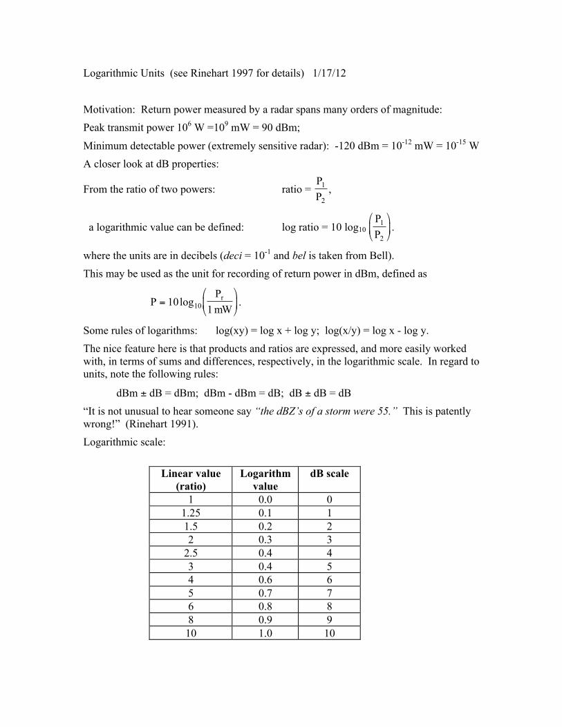
Logarithmic Units (see Rinehart 1997 for details) 1/17/12

Motivation: Return power measured by a radar spans many orders of magnitude: Peak transmit power 106 W =109 mW = 90 dBm;

Minimum detectable power (extremely sensitive radar): -120 dBm = 10-12 mW = 10-15 W A closer look at dB properties:

From the ratio of two powers: ratio = PP1

2,

a logarithmic value can be defined: log ratio = 10 log10 PP1

2

!

"#

$

%& .

where the units are in decibels (deci = 10-1 and bel is taken from Bell). This may be used as the unit for recording of return power in dBm, defined as

PPmWr=

!

"#

$

%&10

110log .

Some rules of logarithms: log(xy) = log x + log y; log(x/y) = log x - log y. The nice feature here is that products and ratios are expressed, and more easily worked with, in terms of sums and differences, respectively, in the logarithmic scale. In regard to units, note the following rules:

dBm ± dB = dBm; dBm - dBm = dB; dB ± dB = dB “It is not unusual to hear someone say “the dBZ’s of a storm were 55.” This is patently wrong!” (Rinehart 1991). Logarithmic scale:

Linear value

(ratio) Logarithm

value dB scale

1 0.0 0 1.25 0.1 1 1.5 0.2 2 2 0.3 3

2.5 0.4 4 3 0.4 5 4 0.6 6 5 0.7 7 6 0.8 8 8 0.9 9 10 1.0 10

1/13/14

1

Radar equation review

1/19/10

Radar eq (Rayleigh scatter)

€

P r =π 3

16 ⋅ 64 ⋅ ln 2$

% &

'

( ) ⋅

PtG2θφhλ2

$

% &

'

( ) ⋅

K 2

r 2 vol∑ Di

6$

% & &

'

( ) )

= c ⋅K 2

r 2⋅Z

The only variable is h, the pulse length Most radars have a range of h values.

€

Z = c3P rr2Rewrite the radar eq as:

Convert to log form:

€

Z = C3 + P r + 20log10(r)

1/13/14

2

Radar equation, Mie scatter

€

P r =1

π 2 ⋅16 ⋅ 64 ⋅ ln 2$

% & '

( ) ⋅ PtG

2λ2θφh[ ] ⋅ 1r 2 vol∑ σ i

$

% &

'

( )

= c'⋅ ηr 2

Uses of the radar equation

•  Convert Pr to Z •  Used for specifications, such as

minimum detectable signal (minimum detectable reflectivity at some standard range)

•  The general form of the radar equation also applies to sodars and lidars

1/13/14

3

Important radar parameters •  Wavelength (cm vs mm) •  Peak transmit power •  Pulse vs. continuous wave (CW) •  Pulse length •  Pulse repetition frequency •  Beam width •  Minimum detectable signal •  Duty cycle: PW/PRT or Pavg/Ppeak •  Receiver bandwidth •  Antenna size (gain) •  Scan rate

Lidar equation

•  But, additional terms representing absorption and extinction are important.

1/13/14

4

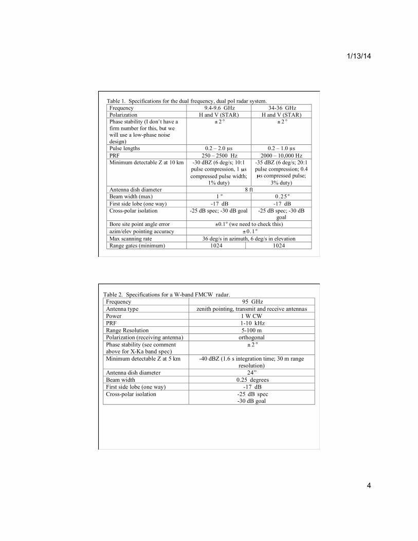
Table 1. Specifications for the dual frequency, dual pol radar system. Frequency 9.4-9.6 GHz 34-36 GHz Polarization H and V (STAR) H and V (STAR) Phase stability (I don’t have a firm number for this, but we will use a low-phase noise design)

± 2 ° ± 2 °

Pulse lengths 0.2 – 2.0 s 0.2 – 1.0 s PRF 250 – 2500 Hz 2000 – 10,000 Hz Minimum detectable Z at 10 km -30 dBZ (6 deg/s; 10:1

pulse compression, 1 s compressed pulse width;

1% duty)

-35 dBZ (6 deg/s; 20:1 pulse compression; 0.4

s compressed pulse; 3% duty)

Antenna dish diameter 8 ft Beam width (max) 1 ° 0 .25° First side lobe (one way) -17 dB -17 dB Cross-polar isolation -25 dB spec; -30 dB goal

-25 dB spec; -30 dB

goal Bore site point angle error ±0.1° (we need to check this) azim/elev pointing accuracy ±0.1° Max scanning rate 36 deg/s in azimuth, 6 deg/s in elevation Range gates (minimum) 1024 1024

Table 2. Specifications for a W-band FMCW radar. Frequency 95 GHz Antenna type zenith pointing, transmit and receive antennas Power 1 W CW PRF 1-10 kHz Range Resolution 5-100 m Polarization (receiving antenna) orthogonal Phase stability (see comment above for X-Ka band spec)

± 2 °

Minimum detectable Z at 5 km -40 dBZ (1.6 s integration time; 30 m range resolution)

Antenna dish diameter 24” Beam width 0.25 degrees First side lobe (one way) -17 dB Cross-polar isolation -25 dB spec

-30 dB goal

1/13/14

5

Beam width estimate

€

θ1 =1.27λD

For D = 8 ft (2.44 m): if λ = 3.2 cm, then θ = 1.27(0.032)/2.44 * 57.3 = 0.95 deg

if λ = 8.6 mm, then θ = 1.27(0.0086)/2.44 * 57.3 = 0.26 deg For D = 2 ft (0.61 m):

if λ = 3.2 mm, then θ = 1.27(.0032)/0.61 * 57.3 = 0.38 deg 3.2 cm 9.4 GHz 8.6 mm 35 GHz 3.2 mm 94 GHz

These are estimates; need to conduct test on antenna range to get actual value

Radial profile of Zmin for WSR-88D

At 50 km: Z = 58.4 dB + (-107 dBm) +20 log10(50) = -20.6 dBZ. At 10 km: Z = 58.4 +(-107) + 20log10(10) = -28.6 dBZ.

-45.0

-40.0

-35.0

-30.0

-25.0

-20.0

-15.0

-10.0

-5.0

0.0

0 10 20 30 40 50 60 70 80 90 100

Range (km)

Δr = 2 km

end

2 -42.64 -36.66 -33.08 -30.5

10 -28.612 -27.014 -25.716 -24.518 -23.520 -22.622 -21.824 -21.026 -20.328 -19.730 -19.132 -18.534 -18.036 -17.538 -17.040 -16.642 -16.144 -15.746 -15.348 -15.050 -14.652 -14.354 -14.056 -13.658 -13.360 -13.062 -12.864 -12.566 -12.268 -11.970 -11.772 -11.574 -11.276 -11.078 -10.880 -10.582 -10.384 -10.186 -9.988 -9.790 -9.592 -9.394 -9.196 -9.098 -8.8

-45.0

-40.0

-35.0

-30.0

-25.0

-20.0

-15.0

-10.0

-5.0

0.0 0 10 20 30 40

100 -8.6

1/17/12

50 60 70 80 90 100

Noise 1/17/12

Schematic of the absorbing elements that need to be considered when estimating the system noise temperature, Tsy, at the receiver input. The waveguide path may also contain other components, such as rotary joints, that have additional losses. While a clear sky is assumed here, it should be noted that rain and clouds add to effective sky noise temperature (increased atmospheric emission of microwave radiation). Taken from Fig. 3.10 of Doviak and Zrnic (1993).

Sources of noise in a radar Refer to Fig. 3.10, D&Z (see above) Noise power of an attenuating radar component Pn = kTBn(1-l-1) (3.31) l is loss factor – ratio of the power in to power out of the component T is temperature of the component in K k = 1.38 x 10-23 W s K-1 is Boltzmann constant Bn is noise bandwidth of the component Physical interpretation: thermal agitation of electrons in the walls of the

component Pn expressed in dB: l = log-1(L/10)

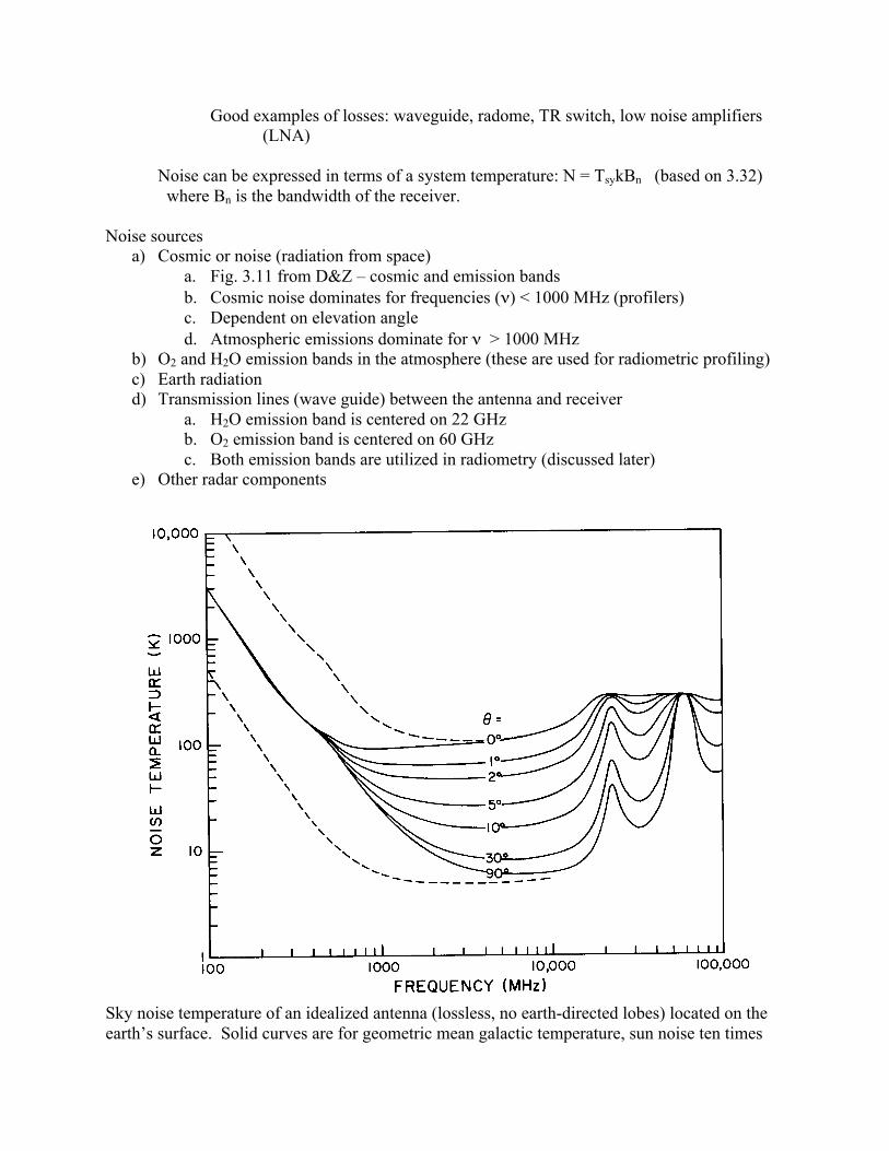
Good examples of losses: waveguide, radome, TR switch, low noise amplifiers (LNA)

Noise can be expressed in terms of a system temperature: N = TsykBn (based on 3.32) where Bn is the bandwidth of the receiver. Noise sources

a) Cosmic or noise (radiation from space) a. Fig. 3.11 from D&Z – cosmic and emission bands b. Cosmic noise dominates for frequencies (ν) < 1000 MHz (profilers) c. Dependent on elevation angle d. Atmospheric emissions dominate for ν > 1000 MHz

b) O2 and H2O emission bands in the atmosphere (these are used for radiometric profiling) c) Earth radiation d) Transmission lines (wave guide) between the antenna and receiver

a. H2O emission band is centered on 22 GHz b. O2 emission band is centered on 60 GHz c. Both emission bands are utilized in radiometry (discussed later)

e) Other radar components

Sky noise temperature of an idealized antenna (lossless, no earth-directed lobes) located on the earth’s surface. Solid curves are for geometric mean galactic temperature, sun noise ten times

the quiet level, sun in unity gain sidelobe, cool temperate zone troposphere, and 2.7 K cosmic black body radiation. The upper dashed curve depicts maximum galactic noise (center of galaxy, narrow beam antenna), sun noise 100 times quiet level, zero elevation angle, and other factors the same as for the solid curves. The lower dashed curve is for minimum galactic noise, zero sun noise, and an elevation angle of 90 deg. The maxima at 22 and 60 GHz are due to water vapor and oxygen absorption resonances. Taken from Fig. 3.11 of Doviak and Zrnic (1993). Power loss is physically related to the thermal agitation of electrons in the walls of the device that confine or guide the electromagnetic waves. Total noise expressed in terms of Tsy, Eq. (3.33) Tsy = Ts(lrlll1)-1 + Tr(lll1)(1-lr

-1) + Tlll-1(1-ll

-1) + Tl(1-ll-1) + TR. (3.33)

Ts – sky noise temperature due to cosmic and atmospheric radiation Tr – radome temperature (usually set at environmental temperature of 290 K) Tl – transmission line temperature (usually set at environmental temperature of 290 K) T1 – T/R switch temperature (usually set at environmental temperature of 290 K) Refer to Fig. 3.10 Signal to Noise Ratio, SNR Ratio of peak return power to noise power SNR = [I2(0) + Q2(0)]erf2[aB6τ/2]/kTsyBn (3.38) B6 – radar bandwidth, defined as the power gain within 6 dB of the highest level The error function (erf) is defined by

and has the form shown below (http://mathworld.wolfram.com/Erf.html). .

SNR for distributed scatterers:

222

0

6

2

6622

0 1)coth( τ

η

ττ

ττ

η

lrC

BaBaB

lrCSNR ∝$

%

&'(

)−=

where C0 is the radar constant. If B6τ is constant, then SNR is proportional to the square of the transmitted pulse length, τ. This comes at the cost of decreasing resolution. The relation to minimum detectable signal (MDS), typically expressed in dBm, is a measure of radar performance. Can also express sensitivity in terms of reflectivity factor, dBZ, at a standard range such as 50 km. Examples: WSR-88D -113 dBm -20.7 dBZ WSR-74C -108 dBm -10 dBZ ARMOR -114 dBm -15 dBZ Aside: Radomes Necessary for weather protection of the antenna and dish system Eliminates variable wind loading on the dish as is rotates. Also keeps water coating off of the reflector. This reduces wear on the mechanical components of the antenna drive bearings and motors. http://www.radome.net/dsfradome.html Two important points regarding radomes:

a) Signal loss through the radome – minimal if a good material is used. A dielectric material is used. Some materials include:

a. Fiberglass b. Sandwich foam

http://www.esscoradomes.com/html/products_sandwich_radomes.html http://www.goreelectronics.com/products/specialty/Radome.html

b) Beam distortion caused by the radome – can be appreciable if metal bolts are used. c) Increased attenuation occurs when the radome is water coated.

http://www.cytonix.com/honeywell.html http://www.radome.net/hydropho.html http://www.esscoradomes.com/html/tutorial_hydro.html Water coating can be minimized by treating the radome with a hydrophobic (water repelling) material, as is typically done (e.g., ARMOR) http://www.radome.net/hydropho.html

Aside: radar absorbing material

Definition: dielectric

DIELECTRIC Pronunciation: ̀ dIi'lektrik

WordNet Dictionary

Definition: [n] a material such as glass or porcelain with negligible electrical or thermal conductivity

Synonyms: insulator, nonconductor Antonyms: conductor

\Webster's 1913 Dictionary

Definition:

\Di`e*lec"tric\, n. [Pref. dia- + electric.] (Elec.) Any substance or medium that transmits the electric force by a process different from conduction, as in the phenomena of induction; a nonconductor. separating a body electrified by induction, from the electrifying body.

1/13/14

Note on reflectivity measurements: The power measurement for distributed scatterers exhibits rapid temporal variation due to variations in relative position of distributed scatterers. The relative fluctuations are very high (orders of magnitude) for successive pulses, separated by the pulse repetition period. Therefore, one needs to average successive pulses to obtain a reasonable return power estimate for a given range gate. This can be accomplished using either temporal averaging (a number of pulses), or a combination of temporal and spatial averaging, as is the case for the WSR-88D (see table below). For the former, in order to obtain a power estimate within about 1 dB accuracy, approximately 50 time samples require averaging.

Fig. 6.2. Standard error of Z estimates (for SNR>>1) vs number of samples, M, with normalized spectrum width σvn a a parameter. From Doviak and Zrnic (1993). For the WSR-88D, the following is used to obtain power estimates for the PRF corresponding to Rmax = 234 km (taken from Table 6.1 of Doviak and Zrnic 1993):

Reflectivity factor calculator Algorithm\ Power average Accuracy of estimate 1 dB Number of samples averaged 6-64 Number or range gates averaged 4 (8) Range increment 1 (2 km)

Time to independence, or decorrelation time: the time it takes hydrometeors to become rearranged such that the samples are independent. Correlation between successive samples is 0.01. Decorrelation time depends on:

a) radar wavelength (shorter to shorter wavelength radars)

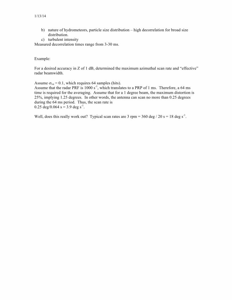
1/13/14

b) nature of hydrometeors, particle size distribution – high decorrelation for broad size distribution.

c) turbulent intensity Measured decorrelation times range from 3-30 ms. Example: For a desired accuracy in Z of 1 dB, determined the maximum azimuthal scan rate and “effective” radar beamwidth. Assume σvn = 0.1, which requires 64 samples (hits). Assume that the radar PRF is 1000 s-1, which translates to a PRP of 1 ms. Therefore, a 64 ms time is required for the averaging. Assume that for a 1 degree beam, the maximum distortion is 25%, implying 1.25 degrees. In other words, the antenna can scan no more than 0.25 degrees during the 64 ms period. Thus, the scan rate is 0.25 deg/0.064 s = 3.9 deg s-1. Well, does this really work out? Typical scan rates are 3 rpm = 360 deg / 20 s = 18 deg s-1.

1313SEPTEMBER 2002AMERICAN METEOROLOGICAL SOCIETY |

uring the Radar Calibration Workshop at the81st Annual Meeting of the American Meteo-

` rological Society in Albuquerque, New Mexico,in January 2001, I was surprised at the relatively littleattention given to some of the simplest and provenmethods. This stimulated some extemporaneous re-marks that I presented toward the end of the work-

AFFILIATION: ATLAS—NASA Goddard Space Flight Center,Greenbelt, MarylandCORRESPONDING AUTHOR: David Atlas, Distinguished VisitingScientist, NASA Goddard Space Flight Center, Code 910,Greenbelt, MD 20771E-mail: datlas@radar.gsfc.nasa.gov

In final form 22 May 2002©2002 American Meteorological Society

D

RADAR CALIBRATIONSOME SIMPLE APPROACHESSOME SIMPLE APPROACHESSOME SIMPLE APPROACHESSOME SIMPLE APPROACHESSOME SIMPLE APPROACHES

In considering new and promising methods to calibrate radar, it is worth remembering some of the

old and perhaps forgotten methods that were used over the last half century.

BY DAVID ATLAS

shop. While formalizing these remarks in writing Ithought it would be useful to elaborate upon them anddiscuss some newer approaches. Thus this paper at-tempts to synthesize a range of techniques. A com-mon thread that runs throughout is the calibration ofthe overall system by use of standard or well-definedtargets external to the radar.

In part, I was troubled by the apparent lack of fa-miliarity of some of the younger generation with earlyactivities in this realm. I was also reacting to the re-cent findings of the variability in the calibrations ofthe Weather Surveillance Radars-1988 Doppler(WSR-88Ds) around the nation that have been uncov-

Above: In the early 1970s, Atlas used BBs to cali-brate the vertically pointing frequency modulated-continuous wave (FM-CW) radar.

1314 SEPTEMBER 2002|

ered by comparison with the radar measurements ofprecipitation by the radar on board the Tropical Rain-fall Measuring Mission (TRMM); (Bolen andChandrasekar 2000). The remarkable stability of theTRMM precipitation radar has made it a travelingstandard against which ground-based weather radarscan be calibrated.

There were a few papers presented at the work-shop that resorted to the more traditional methodssuch as calibration with a standard target. DavidBrunkow of Colorado State University spoke aboutthe use of a metal sphere. Ron Rinehart of the Uni-versity of North Dakota used an oscillating dihedralcorner reflector. Also Isztar Zawadzki recounted hiswork with rain gauges and a Joss–Waldvogel (J–W)disdrometer. Surely, few of the participants wereaware that the early workers in Canada (StewartMarshall, Bob Langille, and Walter Palmer) and inmy group at the Air Force Cambridge Research Labo-ratories (Vernon Plank, Al Chmela, and I) used fil-ter papers powdered with Gentian violet dye (whichleft purple stains on our clothes and teeth) to mea-sure the sizes of tens of thousands of drops by handin the late 1940s and early 1950s (Hitschfeld 1986).Oh what a blessing it was to display the drop size dis-tribution in a comfortable laboratory , while the J–W disdrometer was observing the size of each dropautomatically outdoors.

Historically, it was the Weather Radar Group at theMassachusetts Institute of Technology (MIT), underthe leadership of Alan Bemis and the seminal workby Polly Austin and Ed Williams (1951), that foundthe large underestimates of the radar echoes fromgauge measurements of rain in comparison to thethen-available theory. It was this difference that mo-tivated Richard Probert-Jones (1962) in England toformulate the proper radar equation for meteorologi-cal scatterers (Hitschfeld 1986). For almost a decadewe all struggled to understand the source of this dis-crepancy. And here we are today still struggling withthe optimum methods of radar calibration.

CALIBRATION METHODS. Frequency shift re-flector (FSR). The FSR was invented by John Chisholm(1963). It has been used mainly as a ground-basedtarget for precise locations on airports and geographi-cal siting. It employs a parabolic reflector with a hornat the focus that is shorted by a diode at a frequency f(e.g., 30 or 60 MHz). The frequency f is generated bya battery-driven modulator. The echo from the tar-get is returned at F ± f, where F is the transmitted fre-quency. The echoes at ± f are exactly 6 dB below thatcorresponding to the known cross section of the an-

tenna. These frequencies are readily distinguishedfrom ground clutter and precipitation echoes. It is anexcellent calibration device because it is always avail-able regardless of the weather.

BBs. We first used BBs fired vertically from a BB pis-tol as standard targets to calibrate the vertically point-ing frequency modulated-continuous wave (FM-CW)radar at the Naval Electronics Laboratory Center atPoint Loma, California (Stratmann et al. 1971). Afterhaving failed to support a calibration sphere from aballoon in a stable position on the axis of the radarbeam we searched for another approach. In a jokingmanner I suggested the use of a BB gun. Althoughthere was no prior literature on the subject it wascheap, straightforward, and worth a try. We were verypleased by how well it worked. If enough BBs are used(one at a time), the statistics of echo strength mimicthe radiation pattern of the beam. The maximum echocorresponds to the antenna gain on the beam axis.When using a conventional radar, one should tilt thebeam close to the horizon outside the region ofground clutter. With Doppler radar, the Doppler shiftcan be used to distinguish the moving BBs fromclutter.

Metalized Ping-Pong balls. This is an extension of theBB method. One can fly a light aircraft across andabove a fixed radar beam and drop the balls sequen-tially at about 10–15 m intervals so that only one tar-get is in the beam at any time. The metalized ballsare good targets of known radar cross section. Thesuccessive echoes present a quantitative measure ofthe antenna pattern. Tracking of the aircraft andtiming of each drop positions each target relative tothe maximum echo on the beam axis. The Ping-Pong balls are cheap and nonhazardous. One mayalso use metalized wiffle balls (with holes in them).The idea is to prevent either type of ball from fallingfast enough to create a hazard. Note that either ofthese types of balls may be within the Mie regiondepending on the radar wavelength so that theircross sections should be computed carefully. It is alsopossible to release such targets sequentially from abucket carried on a constant-level balloon movingwith the winds perpendicular to the fixed radarbeam. A similar method was used to measure thecross section of a free-falling artificial hailstone re-leased from a balloon and measured by a trackingradar (Willis et al. 1964).

Airborne modulated target. This approach combines theconcepts in the frequency shift reflector (FSR) and

1315SEPTEMBER 2002AMERICAN METEOROLOGICAL SOCIETY |

Standard Target Radar (STADAR; Atlas 1967).STADAR employs a rotating standard target on theaircraft that modulated the total echo of the aircraftand the target at a frequency corresponding to therotation frequency. The original idea was aimed at usinga simple CW radar to detect the range to the target bythe intensity of the echo from the rotating target ofknown cross section using the radar equation to com-pute the range. However, it would be greatly improvedby using an FSR on board the aircraft so that the echois returned at a frequency that is different from that ofthe carrier frequency and thus separated from the air-craft echoes.

Balloon-borne or airborne standard target. This is an oldscheme that must go back to World War II. However,we first used it in 1953 when we suspended a metal-ized sphere below a helicopter and carried it acrossthe beam of our 24-GHz radar in a study of the radarcharacteristics of fog (Atlas et al. 1953). That studywas aimed at determining the relationship of the ra-dar reflectivity to the liquid water content and dropsizes of fog. Many others have used this method butfound it difficult to track the target in a narrow beam.At the present time the use of the global positioningsystem (GPS), either on the balloon or the airplane,would facilitate tracking.

Calibration with a 24-in. metal sphere suspendedfrom a balloon was done quite reliably by Atlas andMossop (1960) by tracking the balloon with a long,easily identified tail by theodolite. Today one mightmount a television camera on the bore sight axis ofthe antenna and use the wide angle lens to find theballoon and then change to telephoto mode to find itaccurately and adjust the radar position accordingly.

Metalized spherical target released from aircraft. Duringexperiments at Wallops Island, Virginia, to measurethe cross sections of individual insects and birds, thelatter targets were released from an aircraft flying intothe wind while being tracked by the radar (Gloveret al. 1966). The targets were released on countdownand the tracking gate was stopped until the aircraftmoved out of the gate and the unknown target couldbe gated and tracked. Then the aircraft moved upwindwhile the target moved downwind. This approachrequires the use of a tracking radar that can controlthe weather radar. A metalized spherical, constant-altitude balloon can be released from the aircraft andexpanded upon release by the use of a gas cartridge.

Tethered balloon or kytoon. Many investigators haveused metal spheres of known cross section suspended

from tethered balloons or kytoons. Some have usedthree tethers to stabilize the position of the balloon.During experiments in England we used a tetheredballoon with a standard 12 in. diameter metal sphereand an ice ball (i.e., a simulated hailstone) of unknowncross section suspended below the balloon at a suffi-cient vertical spacing to separate the known and un-known targets. Swinging the beam from one to theother allowed us to measure the cross section of thesimulated hailstone with accuracy of better than ~0.5dB. This was more easily done at the time because ofthe use of relatively wide beam height-finder radarssuch as the MPS-4 and the TPS-10 (Atlas et al. 1960).For greater use it is best to do this in the light windsof early morning or evening.

Use of a radar profiler and disdrometer. The use of aDoppler radar profiler (at vertical incidence) along-side a disdrometer allows the measurement of thedrop size distribution (DSD) at the surface, computa-tion of its associated value of reflectivity, and compari-son to the reflectivity measured by the radar at heightsof 300–400 m just beyond the radar recovery time.This calibrates the radar remarkably well. The methodwas first used by Joss et al. (1968). They measured thereflectivity at a height of only 200 m above their zenithpointing radar while measuring the rain and DSD withgauges and a disdrometer. In 46 periods of uniformstratiform rain they found excellent agreement betweenthe actual and the disdrometer-deduced values of Z witha standard deviation of only 6% or 0.25 dB in the ratiobetween the two. It is also remarkable that the radarcalibration was maintained to this accuracy for a pe-riod of 4 months.

This approach has been extended by Gage et al.(2000) and others. An analogous technique is that ofKollias et al. (1999), who used a vertically pointing94-GHz Doppler radar. At this frequency the Miebackscatter function results in a well-defined mini-mum in the Doppler spectrum at a specific drop size.The difference between the measured Doppler speedand the known fall speed for that drop size in still airis then a measure of the air motion; hence, the Dop-pler spectrum in still air may be recovered and theDSD and its reflectivity may be computed. The abso-lute number of drops depends upon the overall radarcalibration and the attenuation by the rain. Thus onestill needs to use a disdrometer adjacent to the radarto account for the attenuation. Once the zenith point-ing radars are calibrated in this fashion, they may beused as transfer standards for other radars.

Ulbrich and Lee (1999) have used the reflectivitycomputed from drop size distributions measured with

1316 SEPTEMBER 2002|

a disdrometer at the surface to check the calibrationof the WSR-88D at Greer, South Carolina, about60 km away from their site at Clemson University.They found that the radar gain was consistently 5 dBtoo low. This is a straightforward technique, particu-larly when used in relatively steady rainfall when thebright band is high. It is similar to the schemes usedby Joss et al. (1968) and that reported by Zawadzki atthis workshop.

Measurement of DSD by aircraft. One may use obser-vations of the drop size distribution on board an air-craft for comparison to ground-based radar measure-ments. This has been done by Marks et al. (1993) tocalibrate and obtain the Z–R relation in a hurricane.In the latter case, the radar was on board the aircraftand measured the reflectivity at a modest distanceahead. The DSD was then measured a few minuteslater as the aircraft penetrated the radar-measuredlocation.

After 56 years of research in radar meteorology, wehave still failed to find a reliable and universally ap-plicable method of radar calibration. Various radarconfigurations require different approaches. I hopethat this brief essay will serve as a menu of simplemethods to fit the needs of various investigators andoperational users.

ACKNOWLEDGMENTS. I appreciate the discussionswith Dr. Merrill Skolnik, former Superintendent of theRadar Division of the Naval Research Laboratories. He re-mains skeptical about the accuracy that may be achievedby some of the techniques described. This work was doneunder the aegis of the NASA Tropical Rainfall MeasuringMission.

REFERENCESAtlas, D., 1967: STADAR, standard target radar. U. S.

Patent No. 3,357,014.——, and S. C. Mossop, 1960: Calibration of a weather

radar by using standard target. Bull. Amer. Meteor.Soc., 41, 377–382.

——, W. H. Paulsen, R. J. Donaldson, A. C. Chmela, andV. G. Plank, 1953: Observation of the sea breeze by1.25 cm radar. Proc. Conf. on Radio Meteorology,Austin, TX, Amer. Meteor. Soc., Paper XI-6.

——, W. G. Harper, F. H. Ludlam, and W. C. Macklin,1960: Radar scatter by large hail. Quart. J. Roy. Me-teor. Soc., 86, 468–482.

Austin, P. M., and E. L. Williams, 1951: Comparison ofradar signal intensity with precipitation rate.Weather Radar Research Tech. Rep. 14, Dept. ofMeteorology, Massachusetts Institute of Technology,43 pp.

Bolen, S. M., and V. Chandrasekar, 2000: Quantitativecross validation of space-based and ground-basedradar observations. J. Appl. Meteor., 39, 2071–2079.

Chisholm, J., 1963: Frequency shift reflector. U.S. PatentNo. 3,108,275.

Gage, K. S., C. R. Williams, P. E. Johnston, W. L.Ecklund, R. Cifelli, A. Tokay, and D. A. Carter, 2000:Doppler radar profilers as calibration tools for scan-ning radars. J. Appl. Meteor., 39, 2209–2222.

Glover, K. M., K. R. Hardy, T. G. Hardy, W. N. Sullivan,and A. S. Michael, 1966: Radar observations of insectsin free flight. Science, 154, 967–972.

Hitschfeld, W., 1986: The invention of radar meteorol-ogy. Bull. Amer. Meteor. Soc., 67, 33–37.

Joss, J., J. C. Thams, and A. Waldvogel, 1968: The accu-racy of daily rainfall measurements by radar. Pre-prints, 13th Radar Meteorology Conf., Montreal, QC,Canada, Amer. Meteor. Soc., 448–451.

Kollias, P., R. Lhermitte, and B. Albrecht, 1999: Verti-cal air motion and rain drop size distributions inconvective systems using a 94 GHz radar. Geophys.Res. Lett., 26, 3109–3112.

Marks, F. D., Jr., D. Atlas, and P. T. Willis, 1993: Prob-ability matched reflectivity–rainfall relations for ahurricane from aircraft observations. J. Appl. Meteor.,32, 1134–1141.

Probert-Jones, J. R., 1962: The radar equation in meteo-rology. Quart. J. Roy. Meteor. Soc., 88, 485–495.

Stratmann, E., D. Atlas, J. H. Richter, and D. R. Jensen,1971: Sensitivity calibration of a dual-beam verticallypointing FM-CW radar. J. Appl. Meteor., 10, 1260–1265.

Ulbrich, C. W., and L. G. Lee, 1999: Rainfall measure-ment error by WSR-88D radars due to variations inZ–R law parameters and radar constant. J. Atmos.Oceanic Technol., 16, 1017–1024.

Willis, J. R., K. A. Browning, and D. Atlas, 1964: Radarobservations of ice spheres in free fall. J. Atmos. Sci.,21, 103–108.