radar interference blanking in radio astronomy …bjeffs/publications/dong_rs_05.pdfradio science,...

Radio Science, Volume ???, Number , Pages 1?? ,

Radar Interference Blanking in Radio Astronomy usinga Kalman TrackerW. DongDepartment of Electrical and Computer Engineering, Brigham Young University, Provo, UT, USA

B. D. JeffsDepartment of Electrical and Computer Engineering, Brigham Young University, Provo, UT, USA

J. R. FisherNational Radio Astronomy Observatory, Green Bank Observatory, WV, USA

Radio astronomical observations of highly Doppler shifted spectral lines of neutralhydrogen and the hydroxyl molecule must often be made at frequencies allocated topulsed air surveillance radar in the 1215-1350 MHz frequency range. The Green Banktelescope (GBT) and many other observatories must deal with these terrestrial signals.Even when strong radar fixed clutter echoes are removed, there are still weaker aircraftechoes present which can corrupt the data. We present an algorithm which improvesaircraft echo blanking using a Kalman filter tracker to follow the path of a sequence ofechoes observed on successive radar antenna sweeps. Aircraft tracks can be used topredict regions (in azimuth and range) for the next expected echoes, even before they aredetected. This data can then be blanked in real time without waiting for the pulse peak toarrive. Additionally, we briefly suggest an approach for a new Bayesian algorithm whichcombines tracker and pulse detector operations to enable more sensitive weak pulsedetection. Examples are presented for Kalman tracking and radar transmission blankingusing real observations at the GBT.

1. Introduction

The frequency bands of spectral line emissions ofneutral hydrogen (1420.4 MHz) and the hydroxylmolecule (1612.2, 1665.4, 1667.4, and 1720.5 MHz)from cosmic sources are protected by internationalspectrum allocations, but observed radiation fromvery distant objects is Doppler shifted to much lowerfrequencies due to the expansion of the universe.Some of this radiation is shifted into the 1215-1350MHz frequency range allocated to radar transmis-sions, such as from the ARSR-3 air surveillance sys-tem. These radar signals can overwhelm astronomi-cal observations, and have been reported to be a sig-nificant problem at the Green Bank Telescope (GBT)(see Zhang et al. [2003], Fisher [2001a] and Fisher[2001b]), Arecibo (see Ellingson and Hampson [2003]and Ellingson and Hampson [2002]) and other ob-

Copyright 2005 by the American Geophysical Union.0048-6604/05/$11.00

servatories. However, the radar signal is impulsiveand transient, so for radio astronomy observation,one solution is to “time-blank” by simply not includ-ing radar corrupted data samples during spectrumestimation (Ravier and Weber [2000] Zhang et al.[2003]). Time blanking has also been used to miti-gate the effect of transmissions from mobile wirelesscommunications services (see Leshem and v.d. Veen[1999] Boonstra et al. [2000] Leshem et al. [1999]).Additionally, a non-blanking approach to radar RFImitigation has been proposed where detected pulsesare removed by parametric signal subtraction with-out discarding data (Ellingson and Hampson [2002]).

To illustrate the problem addressed in this pa-per, Figures 1 and 2 present some 1292 MHz datarecorded at the GBT which clearly shows the radarsignal. A detailed description and analysis of thisreal-world data is provided in Fisher [2001a] andFisher [2001b]. This ARSR-3 radar system is lo-cated in Bedford VA, about 104 km from the GBT.The rotating transmit antenna completes a full 360degree sweep in 12 seconds, with a pulse repetition

1

2 DONG, JEFFS, AND FISHER: RADAR INTERFERENCE BLANKING

Time in seconds

Del

ay in

mic

rose

cond

s (r

ange

)

Bearing angle, degrees

1.4 1.6 1.8 2 2.2 2.4 2.6 2.8 3 3.20

100

200

300

400

500

600

700

800

9003.0 9.0 15.0 21.0 27.0 −3.0 −9.0 −15.0 −21.0 −27.0

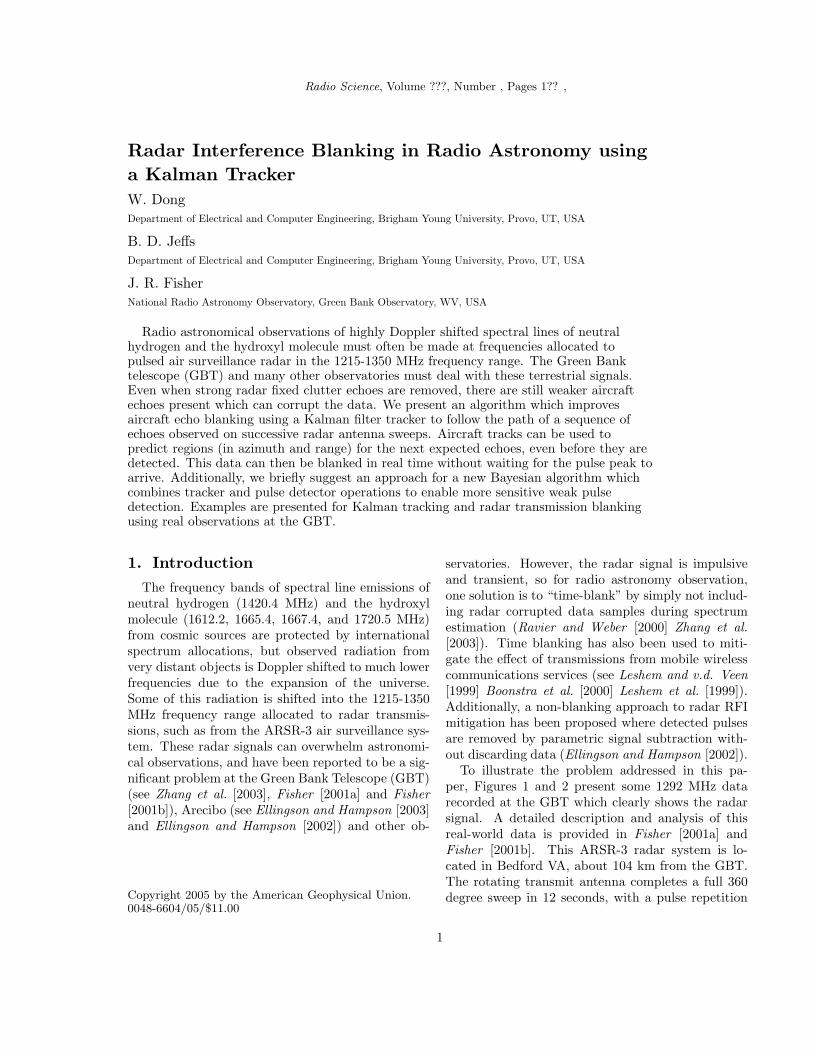
Figure 2. Typical radar sweep time frame as seen atthe GBT. Data are presented in range-azimuth (or equiv-alently range-bearing) map form, with intensity corre-sponding to echo signal power. Zero degrees correspondsto the transmitter beam passing overhead at the GBT.

interval of approximately 2.93 ms and pulse lengthof 3.5 µs.

Figure 1 shows pulse intensity as a function ofdelay relative to the first arriving path for a singletransmitted pulse. Strong signal terms can be seenout to a delay of 135 microseconds, most of whichare due to reflections from the hilly terrain aroundthe GBT (i.e. ground clutter). These can typicallybe excised using fixed time window blanking. Thegroup of echo returns at 430 microseconds is from anaircraft, and blanking it is more problematical sinceit is not present at this same location during eachsuccessive transmit antenna sweep.

Figure 2 gives a two dimensional view of the dataknown as a range-azimuth map. The 1-D time se-ries data has been broken into window blocks andre-ordered so that each transmit pulse, with its asso-ciated echoes, is plotted as a one pixel wide column inthe map. Each column thus contains a 2.93 ms win-dow of received data. The vertical axis representstime between the first detected arrival for a pulseand its longer delayed echoes. Since the transmit an-tenna is rotating, the coarse time horizontal axis canbe interpreted as corresponding to angle (azimuth)of the transmit antenna pointing direction. A 60degree segment of the full sweep is shown, centeredon the time when the transmit beam passes over-head at the GBT. Again two types of radar signals

are seen. Bright regions in the range of 0 to 120µs are fixed echoes from nearby mountainous ter-rain. Bright points at longer delay times are aircraftechoes. Note the wide transmit antenna sidelobe pat-tern for the echo at 310 µs delay.

Receiver Saturation

ARSR-3 Bedford, VA to GBT Bistatic Radar

Rel

ativ

e P

ulse

Inte

nsity

in d

B300 400 500

10

20

30

Delay in microseconds0 100 200

10

Figure 1. Pulse intensity as a function of delay fromthe directly arriving pulse

1.1. Approach

There are two basic approaches to blankingwhich we will call respectively, “time window blank-ing” (TWB) and “detected pulse blanking” (DPB).Strong direct-path pulses and nearby fixed terrainclutter echoes have a predictable repetition cycle andcan be removed by simple TWB. In this approach afixed set of time intervals, synchronized to the radarpulse repetition rate, are removed from the data dur-ing each transmit antenna sweep cycle. All data be-tween the first arrival time and a fixed delay (of forexample 135 µs) is removed for each transmit pulse,eliminating ground clutter echoes and their associ-ated sidelobe structure. TWB is considered the base-line minimum level of radar RFI blanking, and is per-formed on all data sets presented in the remainder ofthis paper. Its effect on the signal seen in Figure 2would be to remove all data in the horizontal bandbetween 0 and 135 µs of delay.

On the other hand, aircraft echoes arrive at arbi-trary times due to aircraft motion, and thus mustbe detected before they can be blanked. DPB isused in this case to remove a window of data in therange-azimuth map surrounding each detected air-craft echo, including transmit antenna beampatternsidelobes which span many transmit pulses.

Two difficulties arise with DPB:

DONG, JEFFS, AND FISHER: RADAR INTERFERENCE BLANKING 3

1. It is very hard to perform blanking in real timebecause aircraft echoes include wide sidelobe pat-terns from the radar transmit beampattern which ex-tend over tens of degrees before and after the centralpeak and over several range bins due to the trans-mit pulse length (see Figure 2). For real-time opera-tion the echo must be anticipated and the full beamsidelobe and pulselength structure must be removedbefore and after the echo peak arrives.

2. Echoes weak enough to make detection of eventhe peak amplitude difficult may still cause signif-icant corruption to the data set. This is becauseastronomical signals of interest are typically tens ofdecibels below the noise floor.

This paper presents a Kalman filter tracker foraircraft echo motion which can be used to resolveboth problems. The proposed method utilizes time-history information across multiple past radar an-tenna sweeps to predict detection locations in thenext upcoming antenna pass. The first problem(real-time blanking) is solved by forming a predic-tion region around an anticipated echo peak to guidedata removal for each affected transmit pulse. Wedesignate this algorithm the “Kalman Detected PulseBlanker” (KDPB).

In a fully digital radio telescope implementationit would be possible to perform real-time blankingwithout KDPB; you could blank pulses stored inmemory as they are detected. However, this requiressufficient memory to handle several seconds of datalatency, and enough computational capacity to keepup with echo detection and tracking while also per-forming the desired scientific analysis. The long la-tency requirement arises from transmit beampatternsidelobes which can precede the detectable centralecho peak by several seconds (see Figure 2).

We propose the alternate solution illustrated inFigure 3. The detection, tracking, and blanking win-dow functions run in parallel with the original signalprocessing path. Using track history information itis possible to predict the next pulse arrival and forma blanking window in advance. This architecture hasseveral advantages over a non-predictive “blank afterdetection” approach.

1. This blanking system may be added to an exist-ing telescope signal path with minimum disruption ofthe current analytical instrumentation or software.

2. It can be applied to both analog or digital in-strumentation because the sampled, digitized dataused for pulse detection and tracking need not be

used for downstream science analysis. The only re-quired system output is the blanking (on – off) con-trol signal.

3. No signal path latency is introduced.

4. Digital sample rates need only support theradar pulse bandwidth. The analytical signal pathmay be broader band, but detection processing re-quires only about a 2 MHz sample rate.

KalmanTracker

BlankingWindowTiming

CLEANDetector

A/DConverter

Blankingswitch

s(t) s'(t)×Original signal path

zn

)ˆ,ˆ( |1|1 nnnn yx ++Sn+1

Parallel predictive blanking algorithm

Figure 3. Processing architecture for predictive real-time blanking. The original instrumentation signal pathis interrupted only by insertion of a blanking switch andtapping of a signal to feed the pulse detector.

This paper will focus on the Kalman tracker basedKDPB solution to the first (i.e. real-time blanking)problem cited above. Its use on real radar transmis-sion data recorded at the GBT will be demonstrated.However, we note that the developed track historycan also be used to form a prior probability distribu-tion for pulse arrivals. This distribution can be usedin a Bayesian framework to improve weak echo de-tection and thus solve the second problem with DPBmentioned above. An improved detection schemecalled “Bayesian-Kalman Detected Pulse Blanking”(BKDPB) will be briefly introduced as another appli-cation for the tracker. The detection theoretic basisfor, and performance analysis of BKDPB will be fullydeveloped in a following paper.

1.2. Data Preprocessing

Before echo pulse tracking can be accomplishedthere are a number of data preprocessing steps whichmust be performed. Details are beyond the scope ofthis space-limited paper (see Dong [2004]), but thebasic operations are listed here for orientation:


100 50 0 50

0

50

100

150

ARSR-3 Bedford, VA to GBT Bistatic RADAR

East coordinate from RADAR, km

Nor

th c

oord

inat

e fr

om R

AD

AR

, km

GBT

ARSR-3

Figure 4. Bistatic geometry of radar signal seen atthe GBT. Echoes from nearby mountains are strong, andhave fixed timing relative to the antenna sweep. Aircraftechoes are non-stationary.

1. Data acquisition was accomplished by samplinga 10 MHz band from the GBT 1.15-1.17 GHz re-ceivers at 20 Msamp/sec. The specifics for the datasets used here are described in Fisher [2001a] andFisher [2001b].

2. A full digital radar receiver was implementedfor optimal pulse detection with unknown time ofarrival, amplitude, and phase. Processing includedcomplex baseband band shifting, band select filter-ing, matched filtering (matched to the transmittedpulse shape), and complex envelope detection.

3. Data was reformatted into time range and az-imuth bins with synchronization to transmit pulseinterval timing. This required careful first arrivalpulse detection and was necessary in order to formrange-azimuth map data presentation for echo posi-tion tracking. This process is fairly complex due toirregular pulse repetition periods and because the re-ceiver and transmitter are non cooperating processes.

4. TWB was applied to blank the first 135 µs ofevery pulse to remove clutter from nearby terrainfeatures.

5. The large extent of an echo in range and az-imuth dimensions can cause many pixels for a singlepulse to exceed the detection threshold. All these

threshold crossings from a single aircraft must begrouped and represented by a single detection cen-troid point. This was accomplished with a modifiedversion of the CLEAN algorithm (Hogbom [1974])which also permits discrimination of distinct echoeswhose sidelobe patterns overlap.

2. Kalman Tracking for InterferingAircraft Echoes

This section presents tracker implementation de-tails. A classical Kalman filter approach as of-ten used for radar target following (see for exam-ple K.V.Ramachandra [2000], Zarchan and Musoff[2000], and Mahafza [2000]) was used with somemodifications specific to the radio astronomy RFIscenario. State equations for aircraft dynamics arerepresented in Cartesian, x − y, coordinates and arethus non-linearly related to the natural polar (rangeand azimuth) coordinate system of the radar detec-tor. This mismatch necessitates use of an extendedKalman filter implementation to linearize the obser-vation data points.

Also, in the RFI case we have a “bistatic” radarscenario where the transmitter and receiver arewidely separated. The ARSR-3 signals seen at theGBT originate at a transmitter site approximately104 km south-southeast of the GBT, as shown inFigure 4. This geometry complicates estimating truephysical range and azimuth relative to the GBT. Az-imuth in all discussions to follow is taken to be rel-ative to the transmitter location, with zero degreesreferenced to when the transmit beam passes directlyoverhead at the GBT. On the other hand, range ismeasured as the two–way bistatic pulse echo traveltime from radar transmitter to the GBT, and is notdirectly proportional to actual distance of the air-craft from either the transmitter or the GBT alone.However, since the goal is not to precisely local-ize each aircraft in real-world coordinates, but tobuild a predictive tracker in any suitable coordi-nate system, we make no attempt to estimate actualrange relative to the GBT. Using the bistatic “pseudorange” measurement does not affect tracker perfor-mance unless the (unknown) observed azimuth anglefrom the GBT to the aircraft is changing rapidly.Tracker computations, including the dynamical mo-tion model, will treat the bistatic pseudo range as anactual geometric range.

The CLEAN algorithm provides isolated detec-tions in range and azimuth, zn = [rn, θn]T , for each


radar antenna sweep. These detections serve as in-puts to the tracker. Here n is the antenna sweep,“snapshot” index for time tn. Also for notationalsimplicity in this discussion we focus on detectionsfrom a single track. The desired tracker outputs atsnapshot n are a prediction point, (xn+1|n, yn+1|n),where the next detection is expected, and shape pa-rameters for an elliptical uncertainty region, Sn+1,centered on this point (see Figure 5). The size ofSn+1 depends on the quality of the track, and getslarger with an increase in observation noise, missedsnapshot detections, or rapid acceleration of the tar-get. Sn+1 selects the region for predictive real-timeblanking, or the region of increased prior probabilityfor an arriving echo pulse for the detection step insnapshot n + 1.

2.1. Dynamic and Observation Models

The tracker employs a position-and-velocity statespace model to describe dynamics of motion for theaircraft. Constant velocity motion perturbed by acorrelated–in–time zero mean Gaussian random pro-cess acceleration vector, an, is assumed. Measure-ments are obtained at discrete sample “snapshot”times, tn, separated by intervals of T seconds. Thedynamic motion model is

xn+1 = Fxn + Gan, where (1)

xn =[xn yn xn yn

]T,

F =

1 0 T 00 1 0 T0 0 1 00 0 0 1

,

G =

[T 2

2 0 T 00 T 2

2 0 T

]T

.

xn is the state vector for a single aircraft, and xn

and xn represent position and velocity respectivelyin the x direction, F is the state transition matrix,and G is the input distribution matrix used to prop-erly update the state vector in response to accelera-tion. an = [ax,n, ay,n]T is the acceleration vector attime snapshot n. Acceleration is viewed as the un-known driving input process to the system modeledby the state equations. In the absence of accelera-tion, the state is updated each snapshot to incrementpositions consistent with constant velocity motion.

The measurement model relates polar observa-tions, zn, to the state equation coordinates and in-

cludes observation measurement noise:

zn = h(xn) + vn, where (2)

h(xn) =[√

x2n + y2

n

tan−1 yn

xn

],

vn = [vr,n, vθ,n]T ,

rn and θn are the measured range and azimuth re-spectively at snapshot n, with corresponding mea-surement noise vr,n and vθ,n.

2.2. Kalman Prediction Equations

Given echo detections and associated track historyup to snapshot n, the first step in a Kalman filter it-eration is to predict the next state vector and updatethe prediction error covariance estimate as follows:

xn+1|n = F xn|n, (3)

P n+1|n = FP n|nF T + GQGT , (4)

−3 −2.5 −2 −1.5 −1 −0.5 0 0.5 1 1.5 2

x 104

2

3

4

5

6

7

8

9x 10

4 x−y coordinate

x (meter)

y (m

eter

)

detectionpredictionestimation

Figure 5. An example of Kalman tracking perfor-mance for data acquired at the GBT. Four aircraft trackshave been automatically established and plotted, includ-ing a pair of crossing tracks. Data from five snapshotsis shown spanning approximately 24 seconds. The fi-nal point plotted for each track is the prediction point,(xn+1|n, yn+1|n). Prediction regions, Sn+1, shown by thedashed ellipses vary in size according to track quality.Note that the center track has a large Sn+1 due to amissed detection. Predictive real-time blanking is accom-plished by excising the prediction region data.


where

xn|n = filtered state estimate at tn

given data through tn,

P n|n = filtered state error covariance,xn+1|n = predicted state estimate,P n+1|n = predicted state error covariance,

Q = acceleration covariance.

xn|n and P n|n are computed using filter equations,(5)–(7), presented in Section 2.3. Note that the pre-diction point, (xn+1|n, yn+1|n), is given by the firsttwo elements of xn+1|n. We define the elliptical re-gion, Sn+1 to be centered on this point and to haveradii rx and ry proportional to

√[P n+1|n]1,1 and√

[P n+1|n]1,1 respectively. Thus the larger the pre-diction error variance, the larger Sn+1 grows to rep-resent our uncertainty as to where the next radarecho will be detected.

Figure 5 illustrates this behavior. The plot showstrack evolution for real GBT data over five snapshotsfor a dense scene with multiple, overlapping aircrafttracks. The ellipses show prediction regions, S6, foreach established track. Note the variety of sizes cor-responding to variations in track quality. For real-time processing these prediction regions are blankedfor the next expected echoes, even before they aredetected. In the BKDPB Bayesian scheme the priorinformation that detections are more likely insidethese ellipses is used for a combined tracking-with-detection algorithm to improve sensitivity to weakpulses.

2.3. Kalman Update (Filter) Equations

When a new snapshot of detections, zn+1, fromCLEAN is available, the Kalman update step com-pletes the iteration begun with equations (3) and (4)as follows:

xn+1|n+1 = xn+1|n + Kn+1

×[zn+1 − h

(xn+1|n

)], (5)

P n+1|n+1 =[I − Kn+1Hn+1

],

×P n+1|n (6)

Kn+1 = P n+1|nHTn+1 (7)

×[Hn+1P n+1|nHT

n+1 + R]−1

,

where the extended Kalman filter linearization abouttn+1 is provided by

Hn+1 =[

∂h

∂x

]x=xn+1|n

(8)

=

1√

x2n+1|n + y2

n+1|n

×[

xn+1|n yn+1|n 0 0−yn+1|n xn+1|n 0 0

],

and where Kn+1 is the Kalman gain matrix.Range estimation error standard deviation is pro-

portional to the pulse length. Azimuth error devi-ation is proportional to antenna beamwidth and isstatistically independent of range error. Thus rangeand azimuth measurement error are properly mod-eled with a measurement error covariance of the sim-ple form

R =[σ2r 00 σ2

θ

], (9)

where there are no cross correlation terms and vari-ances are constant with respect to range and az-imuth. We note that measurement error (noise) mod-eled in the (x, y) domain would not have this simplestructure, would be correlated between x and y, andwould be a function of r. However, with the extendedKalman filter approach the above update equationstake care of this transformation and the proper corre-lated structure is found in error covariance matricesP n+1|n+1 and P n+1|n. After computing (5), (6), and(7), index n is incremented to complete the iterationwhich started with prediction equations (3) and (4).

2.4. Track Initialization and Management

The prediction and update equations include sev-eral parameters that are either assumed known andmust be estimated externally (i.e. Q and R), or areiteratively estimated but need good initial values forstable track start up (P n|n and xn|n). Also, in prac-tical multiple target automatic tracking applicationsit is necessary to deal with a number of ambigui-ties when interpreting the pulse detection data. Wehave developed a set of rule–based procedures (morefully described in Dong [2004]) to address these is-sues. The following list describes our approach forinitializing and managing tracks.

1. State Parameter Initialization. Two succes-sive associated pulse detections are required beforea track can be initiated. x0|0 is initialized with theposition of the second detection, and a two-sample


velocity estimate is computed from the position dif-ference between the detections.To find a practical initialization for P 0|0, we ran thetracker on synthetic detection data which simulatedthe aircraft motion seen in real GBT data. Aftera large number of Monte Carlo random trials, P n|nconverged on average to P∞|∞ ≈ (2 × 103)I. Thisvalue was used to initialize P 0|0 when processing realdata from the GBT.

2. Constant Parameter Estimates. The accelera-tion process covariance is modeled as a constant ma-trix of the form

Q = E{anaTn} =

[σ2

x σ2xy

σ2xy σ2

y

]. (10)

Values of σ2x = σ2

y = 12.0 and σ2xy = σ2

yx = 0 wereused in the results described below and were estab-lished by qualitative analysis of flight paths in thereal GBT data. Parameters were set so that syn-thetically generated tracks in random trials by thestate space model had acceleration rates (turn radii)comparable to what was observed in the real aircraftdetection data. an was generated by lowpass filteringtwo mutually independent Gaussian white noise timesequences (one each for ax(n) and ax(n)). A filtercutoff frequency of fc = 1

100T produced smooth sim-ulated aircraft turning maneuvers which were quali-tatively consistent with real track paths seen in theGBT data.Tracking performance did not appear in practice tobe critically dependent on the values set for σ2

x andσ2

y. However, settings significantly higher (by a fac-tor of two or more) increase the size of the predictionregion, Sn+1 and thus increases likelihood of associ-ating a new detection with the wrong track. Settingthese terms too small results in tracks failing to asso-ciate the new detection with a track when there hasbeen some maneuver, or direction change.For initializing R we note that σ2

r is proportionalto both the receiver noise variance and the square ofthe transmit pulse length. σ2

θ is proportional to noiseand to the square of transmit antenna angular rota-tion rate divided by transmit pulse repetition rate.We have estimated these parameters empirically forthe GBT data and treat them as constants in theKalman update.

3. Track Association. For each new snapshot theCLEAN algorithm produces a set of detections. Eachof these must be classified as being a newly de-tected aircraft for which a track must be created,

or as belonging to an existing track. Detectionswhich lie within a fixed distance, da, from an ex-isting track’s prediction point, (xn+1|n, yn+1|n), areassociated with that track. To avoid ambiguities, de-tections which satisfy this criterion for two or moredistinct tracks are assigned to the track whose pre-diction point is closest.

4. Track Creation. New detections which are notwithin a distance da of any existing prediction pointare designated candidate starting points. The trackis created if in the succeeding snapshot, n + 1, a de-tection within distance dn of the candidate point isfound which is not associated with any existing track.da serves as a bound on how much prediction erroris to be tolerated and is proportional to the maxi-mum radius of Sn+1. dn is a bound on the maximumdistance an aircraft can travel in T seconds, and istypically much larger than da since prediction pointsare expected to be close to the true location. Sinceno velocity or direction information is available froma single candidate point, there will be no predictionpoint at time n + 1, and the candidate track mustaccept any unassociated detection within a radius ofdn from the initial detection.

5. Missed Detections. If in a given snapshot nonew detection is associated with a particular track,it is assumed that the aircraft is still present, but thatthe detection was missed due to random variation inecho amplitude. Consider missing k successive detec-tions for a given track. In this case, Kalman predic-tion equations (1), (3), and (4) from prior snapshot,tn−k, are recomputed as a multi–step prediction byreplacing T with kT . This produces the desired k–step prediction point (xn+1|n−k, yn+1|n−k) but theprediction error covariance, P n+1|n−k, increases andthe size of Sn+1 grows as compared to a normal singlestep prediction.

6. Track Dropping. A track which has no associ-ated detections in three successive snapshots is ter-minated.

7. Track Splitting. If two or more new detec-tions are associated with a single track then thetrack is split into separate tracks for each new de-tection. These split tracks have a common historyfor t ≤ tn−1 but for t ≥ tn are computed as distincttracks. This scenario arises when aircraft paths crossor when a new aircraft detection occurs close to anexisting track prediction point of a different aircraft.


3. A Combined Kalman Tracker andBayesian Detector

In a conventional radar detector, all range-azimuthbins are assumed to be equally likely to contain anecho. Detections are made when the magnitude–squared matched filter output exceeds a predeter-mined constant threshold, τ . Thresholds are set toyield a specified probability of false alarm (PFA). Fora fixed PFA, the probability of detection (PD) is afunction of the receiver design and signal statistics,such as signal to noise ratio.

In the context of the Kalman tracker, one need notassume all bins have the same probability of detec-tion. The track histories provide prior informationwhich indicates a higher probability of echoes beingdetected in prediction regions, Sn+1. We propose aBayesian detection scheme where a spatially depen-dent prior probability density function for the pres-ence of an echo, f(x, y), is computed using the Sn+1

ellipses to designate areas of increased density. Withthis approach it is possible to increase the overall PDwithout an increase in PFA. A detailed theoreticaldevelopment of this detector is found in Dong [2004]and in a forthcoming paper. When used for RFI re-moval we refer to the method as Bayesian-KalmanDetected Pulse Blanking (BKDPB).

Here it is simply noted in summary that with arigorous detection theoretic development it can beshown that the net effect of the Bayesian detectoris to make the detection threshold, τ(x, y), spatiallyvarying, with local minima at the prediction pointcentroids of the Sn+1 regions, as illustrated in Figure8. Section 4 presents a comparison of spectral densityestimates with conventional DPB and the proposed

τ0 τ0

τ(x,y)

τ(x,y)

Prediction point

Figure 8. The threshold τ is determined by the priordistribution f(x, y) of the presence of a pulse. τ0 is theconstant threshold outside the elliptical regions, Sn+1.τ(x, y) is at a local minimum corresponding to each pre-diction point. The two concavities represent decreasedthreshold according to the prior probability inside twodifferent sized Sn+1.

BKDPB. The new method produces less radar pulsebias in the spectral estimate.

4. Experimental Results

Two sets of real data recorded at the GBT for a 10MHz wide band around 1292 MHz were used to testthe echo detection algorithm, tracking, and blankingperformance. Set one was collected in April of 2002,and set two in January of 2003.

Figure 6 presents a typical Kalman tracking resultfor data set one. This example illustrates success-fully tracking 11 aircraft, including crossing tracksand track splitting. A number of other detectionsare seen which have not yet been associated withtracks. Conventional fixed threshold detection wasused here. Throughout this entire data set, the trackprediction regions formed good estimates of the nextecho location, and were suitable for real-time predic-tive blanking (KDPB).

−3 −2 −1 0 1 2 3 4

x 104

0

2

4

6

8

10

12x 10

4 x−y coordinate

x (meter)

y (m

eter

)

t34t35t36t37estimationprediction

Figure 6. Tracking result example for five antennasweep snapshots, t34 to t38. Note that not ever sweepwas used, so the snapshot interval, T , in this case is 60seconds. Ellipses indicate prediction regions for the finalsnapshot.

Figure 7 illustrates effectiveness of the real-timeblanking technique (KDPB). Though processing was


actually performed on recorded data set two, blank-ing regions were based (as they would be for real-time operation) on the Kalman tracker predictionsusing only past history data. This data set includes50 radar antenna rotations. All blanking was imple-mented by “zero-stuffing” , that is, placing zeros intothe time samples where radar transmissions are de-tected (Zhang et al. [2003]). The lower curve showsthat the power spectrum after KDPB is dramaticallyimproved, with lower bias due to radar aircraft echocontamination.

0 1 2 3 4 5 6 7 8 9 100.2

0.25

0.3

0.35

0.4

0.45

0.5

0.55

Frequency in MHz

Rel

ativ

e P

ower

time window blanking ONLYtime window + pulse detected blanking

Figure 7. Power spectrum estimates for two approachesto radar pulse blanking. Only TWB was used for the up-per curve. Both TWB and KDPB were used for the lowercurve. The 1292 MHz radar pulse carrier frequency hasbeen mixed down to about 4 MHz in this plot.

Figure 9 illustrates how the Bayesian-Kalman de-tector in BKDPB can find weaker echoes that wouldbe missed with conventional constant threshold de-tection. These tracks come from data set one andwere computed using BKDPB. The three echoes

marked by rectangles were not detected when thesame data was processed with KDPB.

−1.2 −1 −0.8 −0.6 −0.4 −0.2 0 0.2 0.4 0.6 0.8100

200

300

400

500

600

700

800

900

Detected echoes using new algorithm: t34

−t38

Bearing in seconds

Del

ay in

mic

rose

onds

t34t35t36t37t38

Figure 9. Real data detection results for both algo-rithms for five snapshots from the GBT. Note that 3weaker pulses (inside the rectangles) are missed by theconstant threshold algorithm (DPB), and picked up withBKDPB detection.

0 1 2 3 4 5 6 7 8 9 100.4

0.41

0.42

0.43

0.44

0.45

0.46

0.47

Frequency in MHz

Rel

ativ

e P

ower

KDPBBKDPB

Figure 10. Power spectrum estimate for a segmentof data set two containing two weak echoes. The con-stant threshold detection of KDPB was used for the up-per curve, but no echoes were found. In the lower curvethe Bayesian-Kalman detector in BKDPB located andblanked three echoes and thus reduced radar bias near5.5 MHz.


Figure 10 shows the differnece between spectralestimates computed using the KDPB and BKDPBblanking algorithms. In this particular data windowfrom data set two there were no strong aircraft echoesso KDPB made no detections. There are two weakaircraft echoes which were detected with BKDPBand the corresponding time samples were blanked(set to zero) when computing a power spectrum. Theresulting curve shows reduced bias near 5.5 MHz cor-responding to the radar pulse center frequency. Thelarger deviations at 0 and 10 MHz are not fully un-derstood, but are assumed to be band edge effects.

5. Conclusions

Detected pulse blanking using Kalman filter track-ing techniques has been shown to be an effective ap-proach for real-time radar RFI mitigation. Bias dueto radar pulses in GBT observations was reduced ascompared to to simple fixed time window blanking(TWB). Also, the new Bayesian combined trackingand detection algorithm has been shown to improveblanking of weak aircraft echo pulses, leading to afurther reduction in bias in power spectrum estimatesof the noise floor (see Figures 7 and 10). Multiple si-multaneous tracks were managed (as many as 11) foraircraft seen in real observations at the GBT. Cross-ing tracks, congested traffic regions, and intermittenttrack detections were all handled satisfactorily. Thecomputational load for the tracker is modest since itoperates on detections only and is updated only atthe transmit antenna sweep rate. We have run thetracking portion of the code in MATLAB faster thanreal time using a modest PC. However, the requireddigital radar receiver and pulse detector operate atthe raw baseband signal sample rate and require asignificant digital signal processing platform, thoughsuch systems are widely in use. This paper presentedthe system development and analyzed performanceby post processing previously recorded data. A nextstep is to implement this in a true real-time envi-ronment on our experimental RFI mitigation DSPtest platform. This will permit us to evaluate thetrue impact this system can have on improve radioastronomical observation science.

Acknowledgments. This work is supported bythe National Science Foundation grant number AST-9987339.

ReferencesBoonstra, A., A. Leshem, A.-J. van der Veen,

A. Kokkeler, and G. Schoonderbeek (2000), The effect

of blanking of tdma interference on radio-astronomicalobservations: experimental results, in Proc. of theIEEE International Conf. on Acoust,, Speech, and Sig-nal Processing, vol. 6, pp. 3546–3549.

Dong, W. (2004), Time blanking for gbt data with radarrfi, Master’s thesis, Brigham Young University.

Ellingson, S., and G. Hampson (2002), Rfi and asyn-chronous pulse blanking in the 1230-1375 mhz bandat arecibo, Tech. rep., Ohio State University.

Ellingson, S., and G. Hampson (2003), Mitigation ofradar interfernece in l-band radio astronomy, The As-trophysical Journal Suplement Series, 147, 167–176.

Fisher, J. (2001a), Summary of rfi data samples at greenbank, Tech. rep., National Radio Astronomy Observa-tory, Green Bank Observatory.

Fisher, J. (2001b), Analysis of radar data from february6, 2001, Tech. rep., National Radio Astronomy Obser-vatory, Green Bank Observatory.

K.V.Ramachandra (2000), Kalman Filtering Techniquesfor Radar Tracking, Marcel Dekker.

Leshem, A., and A.-J. v.d. Veen (1999), Introductionto interference mitigation techniques in radio astron-omy, in Perspectives in Radio Astronomy, Technolo-gies for Large Antenna Arrays, edited by A. Smoldersand M. van Haarlem, NFRA, Dwingeloo, The Nether-lands.

Leshem, A., A.-J. v.d. Veen, and E. Deprettere (1999),Detection and blanking of gsm interference in radio-astronomical observations, in Proceedings of the 2ndIEEE Workshop on Signal Processing Advances inWireless Communications, pp. 374–377.

Mahafza, B. (2000), Radar Systems Analysis and DesignUsing MATLAB, Chapman and Hall/CRC Press.

Hogbom, J. (1974), Aperture synthesis with a nonregu-lar distribution of interferometer baselines, Astronomyand Astrophysics Supplement, 15, 417.

Ravier, P., and R. Weber (2000), Robustness in rfi detec-tion for time-blanking, Tech. rep., LESI and ESPEO,University of Orlans, France.

Zarchan, P., and H. Musoff (2000), Fundamentals ofkalman filtering: A practical approach, Progressin As-tronautics and Aeronautics, 190, 257–291.

Zhang, Q., Y. Zheng, S. Wilson, J. Fisher, and R. Bradley(2003), Combating pulsed radar interference in ra-dio astronomy, The Astronomical Journal, 126, 1588–1594.

W. Dong and B. D. Jeffs, Department of Electri-cal and Computer Engineering, Brigham Young Univer-sity, Provo, UT 84602, USA ([email protected], [email protected])

J. R. Fisher, National Radio Astronomy Observa-tory, P.O. Box 2, Green Bank, WV 24944, USA([email protected])

(Received .)

radar interference blanking in radio astronomy …bjeffs/publications/dong_rs_05.pdfradio science,...

Documents