Stojanovic, JASA 1

Retrofocusing techniques for high rate acousticcommunications a)

Milica Stojanovicb)

Massachusetts Institute of Technology

Cambridge, MA 02139

Abbreviated/running title: “Retrofocusing for acoustic communications.”

Received

a)Portion of this work was presented at the High Frequency Ocean Acoustics Conference, March 2004.b)Electronic mail: millitsa@mit.edu

Stojanovic, JASA 2

Abstract

High rate underwater communications have traditionally relied on equalization

methods to overcome the intersymbol interference (ISI) caused by multipath prop-

agation. An alternative technique has emerged in the form of time-reversal, which

comes at virtually no cost in computational complexity, but sacrifices the data rate

and relies on the use of large arrays to reduce ISI. In this paper, spatio-temporal pro-

cessing for optimal multipath suppression is addressed analytically. A communication

link between a single element and an array is considered in several scenarios: uplink and

downlink transmission, with and without channel state information and varying imple-

mentation complexity. Transmit/receive techniques are designed which simultaneously

maximize the data detection SNR and minimize the residual ISI, while maintaining

maximal data rate in a given bandwidth and satisfying a constraint on transmitted en-

ergy. The performance of so-obtained focusing techniques is compared to the standard

ones on a shallow water channel operating in a 5 kHz bandwidth around a 15 kHz cen-

ter frequency. Results demonstrate benefits of focusing techniques whose performance

is not conditioned on the array size. Optimal configurations are intended as a basis

for adaptive system implementation in which channel estimates will replace the actual

values.

PACS numbers: 43.60 (Ac,Dh,Fg,Gk,Tj)

Keywords: underwater acoustic communications, time-reversal, transmit/receive array, op-

timal filtering, equalization.

Stojanovic, JASA 3

I. INTRODUCTION

High rate, bandwidth-e!cient underwater communications have traditionally relied on

adaptive equalization methods to overcome the intersymbol interference (ISI) caused by

multipath propagation. Excellent performance of these receivers comes at a price of high

computational complexity. While processing complexity can be somewhat reduced by use

of sophisticated spatio-temporal multichannel equalizers,1 retrofocusing techniques appear

to o"er a di"erent approach. In traditional equalization, all of the signal processing is

performed at the receiver side, while the transmitter uses standard signaling waveforms,

which are designed a-priori, and, hence, are not matched to the channel. A di"erent, and

possibly better approach results if signal processing can be split between the transmitter and

receiver. Such an approach forms the basis of spatio-temporal retrofocusing.

In its simplest form, retrofocusing is achieved by transmitting a time-reversed (or equiv-

alently, phase-conjugated in the frequency domain) replica of a probe signal received earlier

from the source location. This technique has been used for medical imaging, therapy, and

material testing,2 while more recently, time-reversal has been investigated as a commu-

nication technique that o"ers lower computational complexity as compared to traditional

equalization.3!23 However, in high rate communications time-reversal alone does not elim-

inate ISI, the fact that motivates present analysis and the search for optimal retrofocusing

techniques.

A. Previous work

Several research groups have been involved in application of time-reversal arrays to under-

sea acoustic communications, addressing active phase-conjugation for two-way communica-

tion, as well as passive phase-conjugation for one-way communication from a single-element

source to an array.

The Scripps group has been engaged in experimental work, using large arrays to demon-

strate spatial and temporal focusing of phase-coherent communication signals.3!8 Commu-

nication begins with a single-element source transmitting the initial probe to an array. The

array then uses the time-reversed replicas of the received, channel-distorted probe to generate

Stojanovic, JASA 4

transmit filters that are subsequently used for pulse-shaping the information sequence that

is sent back to the source. This method of two-way communication is called active phase-

conjugation. In one of the experiments, a 30 element array, operating at a center frequency

of 3.5 kHz, was used to transmit PSK signals pulse-shaped at the transmitter array by a

time-reversed replica of the probe signal received earlier. No signal processing was employed

at the receiver, and transmission at 1 kilobit per second over 10 km was reported.

The University of Washington group has addressed experimentally the technique of pas-

sive phase-conjugation,9!13 in which the same principle of time-reversal is used for one-way

communication. In this technique, the single-element source sends a probe, waits for the

channel reverberation to subside, and then transmits the information-bearing signal to the

array. The received channel-distorted probe is time-reversed and used at each array element

as a receive filter for subsequent detection of the information-bearing signal. Periodic in-

sertion of the probe signal is necessary to account for the time-variability of the channel.

The technique was demonstrated experimentally using a 14 element array, operating in the

5 kHz - 20 kHz band, to transmit data over distances of about 1 km. Transmission at 2

kilobits per second was reported; however, such transmission could only be sustained for a

short period of time, after which the probe signal had to be retransmitted to account for the

channel time-variability (probe retransmission e"ectively reduced the data rate by a factor

of two). To recover the loss in data rate, decision-directed phase-conjugation was used, in

which the detected data stream was used to regenerate the channel estimates. Passive phase

conjugation was compared to standard equalization, showing that significant performance

degradation, which increases with SNR and eventually leads to saturation, is the price to be

paid for low computational complexity.14

In parallel with these experimental e"orts that emphasize low-complexity processing using

time-reversal, a third group of researchers at IST, Portugal, focused on analytical work.15!20

Realizing that probe retransmission considerably reduces the e"ective data rate in both active

and passive phase-conjugation, this group proposed the use of adaptive channel estimation to

generate the up-to-date time-reversed filters directly from the received information-bearing

signal, thus eliminating the need for probe retransmission (inevitably at the expense of

increased computational complexity). This group also proposed the use of low-complexity

Stojanovic, JASA 5

adaptive equalization in conjunction with time-reversal.

As the early experiments, devoted to implementing time-reversal in the ocean and testing

the basic concepts have shown, suppression of multipath e"ects through time-reversal can be

achieved at the expense of reduced data throughput and/or the need for a large array. For a

better utilization of channel resources, additional signal processing is necessary to eliminate

ISI and enable high-rate communications.

Ensuring ISI-free transmission in a system that has multiple transmit/receive elements

is a major asset in a channel whose bandwidth is severely limited. In particular, it lays

ground for capacity improvement through the use of space-time coding and multi-input

multi-output (MIMO) signaling. This technique, developed originally for radio channels,

was shown to increase the fundamental channel capacity in proportion to the number of

transmit/receive elements used.24 However, capacity-approaching codes are known only for

ISI-free channels. MIMO signal processing for controlling the intersymbol and the inter-

channel interference in underwater acoustic systems was addressed in the framework of

multiple-user communications,25 and, more recently, for single-user communications using

multiple transmit elements.26 Recent experimental results demonstrate large bandwidth ef-

ficiency improvement over acoustic channels, provided that accurate channel estimation is

available and that residual ISI is kept at a minimum.

B. Problem definition

While recent research demonstrates the potential of time-reversal in spatial localization

of acoustical energy, it often fails to recognize that time-reversal alone does not provide

temporal focusing necessary to eliminate ISI caused by multipath propagation. Time-reversal

recombines multipath energy in a manner of matched filtering, whose function is to maximize

the SNR at a given time instant, and not to eliminate ISI. In fact, matched filtering increases

temporal dispersion of the signal, i.e. the duration of the overall impulse response of the

system. While SNR maximization is an appropriate optimization criterion for single pulse

focusing, its application to communication problems, where a sequence of data-modulated

pulses is transmitted at a high rate, must be approached judiciously. For signals that contain

temporal dispersion, matched filter represents only the front end of the optimal receiver, and

Stojanovic, JASA 6

must be followed by a sequence estimator or an equalizer.27

Multipath components that remain after matched filtering contribute to residual ISI,

whose severity depends on the channel. If not equalized, residual ISI may completely prevent

detection. Increasing the number of array elements in a time-reversal array only helps to

reduce residual ISI, but it does not eliminate it. Hence, if time-reversal is to be used towards

eliminating the multipath distortion without sacrificing the data rate, it must be combined

with equalization to remove residual ISI. However, the advantage of this approach to standard

equalization that uses fixed transmitter waveforms is not apparent. The use of retrofocusing

for complete suppression of multipath thus remains an open question.

In this paper, a solution is proposed to the following problem: If the channel responses

between a single element and an array are known, determine the optimal transmit/receive

technique that the two can use to simultaneously (i) eliminate ISI and (ii) maximize SNR,

while maintaining maximal data rate in a given bandwidth and satisfying a constraint on

transmitted energy. Note that because it allows for transmitter as well as receiver opti-

mization, the solution di"ers from standard equalization. Also, because it explicitly requires

minimization of ISI, it di"ers from time-reversal. The resulting system does not depend on

the number of array elements to minimize the multipath distortion, i.e. it does not trade the

computational complexity for the array size, but instead provides an answer for a variety of

applications that cannot a"ord large arrays.

For those applications that also cannot a"ord processing power at both ends of the

link, a constrained optimization problem is considered. A complexity restriction, likely to

be imposed on the remote, single-element end, forces its transmit/receive filters to use no

knowledge of the channel. The resulting one-sided focusing solution sacrifices some of the

performance of the two-sided focusing in exchange for minimal implementation complexity.

Analytical results are provided to quantify this trade-o".

A related question that emerges during the study of optimal focusing is the following:

If the requirement for no ISI is relaxed, and the use of both channel-dependent transmit

filtering and equalization at the receiver is allowed, what is the optimal system configuration,

and how does its performance compare to that of optimal focusing? Analytical solution to

this problem provides an upper bound on the performance of all spatio-temporal processing

Stojanovic, JASA 7

methods.

System optimization is addressed in Sec. II. under various optimization criteria. In Sec.

III., the performance of resulting techniques is compared through numerical computation

of the analytical expressions for predicted performance of a system operating at 10 kilobits

per second over a 3 km shallow water channel. Results demonstrate the benefits of optimal

focusing which outperforms time-reversal, and whose performance is not contingent on the

array size. The conclusions are summarized in Sec. IV.

Optimal configurations discussed in this paper are intended as a basis for adaptive system

implementation in which channel estimates will replace the unknown, time-varying responses.

An adaptive channel estimation procedure, which uses a low-complexity decision-directed

approach,28 is suitable for this task.

II. SYSTEM OPTIMIZATION

In this section, system optimization is addressed for uplink and downlink communication

(to/from array), as shown in Fig.1. Performance is assessed using SNR as the figure of

merit, and compared to that of time-reversal, standard linear equalization, and transmit

time-reversal in conjunction with equalization (receive time-reversal is identical to matched

filtering, which, when followed by an equalizer, reduces to standard equalization). System

optimization is first addressed under no ISI requirement, while optimization of transmit

filtering for use in conjunction with equalization is addressed subsequently.

A. Transmitter/receiver optimization for no ISI (focusing)

The sequence of data symbols d(n) is transmitted at a symbol rate 1/T . Referring to

Fig.1, the problem is to find the transmit/receive filters G0(f) and G1(f), . . .GM (f) such

that the SNR at the receiver is maximized, subject to the constraint that there is no ISI

in the decision variables d̂(n) = y(nT ), and that finite transmitted energy per symbol E is

used. The channel responses Cm(f), m = 1, . . . M , and the power spectral density Sw(f) of

the uncorrelated noise processes wm(t), m = 0, . . .M , are assumed to be known.

Stojanovic, JASA 8

Let the composite equivalent baseband channel transfer function be denoted by

F (f) = G0(f)M!

m=1

Gm(f)Cm(f). (1)

The received signal after filtering is then given by

y(t) =!

n

d(n)f(t ! nT ) + z(t) (2)

where the noise z(t) has power spectral density

Sz(f) = Sw(f) "

"#$

#%

&Mm=1 |G2

m(f)|, for uplink transmission

|G20(f)|, for downlink transmission .

(3)

The requirement for no ISI is expressed as

F (f) = X(f) (4)

where X(f) is a Nyquist transfer function, i.e., it is bandlimited to |f | < 1/T , and its

waveform in time, x(t), satisfies the condition

x(nT ) =

"#$

#%

x0, for n = 0

0, otherwise .(5)

Without the loss of generality, we take that X(f) = |X(f)|. For example, X(f) can be

chosen as a raised cosine spectrum,27 whose bandwidth B is controlled by the roll-o" factor

! # [0, 1], B = 1T (1 + !). When ! $ 0, X(f) $ T for |f | % 1

2T , and no excess bandwidth is

used, i.e., maximal symbol rate is achieved for which ISI-free transmission is possible within

the available bandwidth.

When there is no ISI, the received signal, sampled at times nT , is given by

y(nT ) = d(n)x0 + z(nT ) (6)

and the SNR is

SNR ="2

dx20

"2z

. (7)

where "2d = E{|d2(n)|} and "2

z =' +"!" Sz(f)df .

The total transmitted energy is the energy of the signal u0(t) =&

n d(n)g0(t ! nT )

for the uplink scenario, or the sum of energies of the signals um(t) =&

n d(n)gm(t ! nT ),

Stojanovic, JASA 9

m = 1, . . . M for the downlink scenario. The power spectral density of these signals is

Sum(f) = 1T Sd(f)|Gm(f)|2, where Sd(f) is the power spectrum of the data sequence.27 If the

transmitted energy per symbol is set to E, assuming uncorrelated data symbols (Sd(f) = "2d),

the energy constraint is expressed as

E = "2d "

"#$

#%

' +"!" |G2

0(f)|df, for uplink transmission&M

m=1

' +"!" |G2

m(f)|df, for downlink transmission .(8)

1. Unrestricted optimization (two-sided filter adjustment)

Let us first consider uplink transmission. Taking into account the energy constraint, and

the no-ISI requirement, G0(f) = X(f)/&M

m=1 Gm(f)Cm(f), the SNR is expressed as

SNR =Ex2

0

"2z

' +"!" |G2

0(f)|df=

=Ex2

0' +"!"

X2(f)

|&M

m=1Gm(f)Cm(f)|2

df' +"!" Sw(f)

&Mm=1 |G2

m(f)|df. (9)

This function is to be maximized with respect to the receive filters Gm(f), m = 1, . . . M . To

do so, we use a two-step procedure, each step involving one Schwarz inequality. The first

inequality states that

|M!

m=1

Gm(f)Cm(f)|2 %M!

m=1

|G2m(f)|

M!

m=1

|C2m(f)| (10)

where the equality holds for

Gm(f) = !(f)C#m(f). (11)

We note similarly with time-reversal in that receive filters should be proportional to the

phase-conjugate of the channel transfer functions. However, there is room for additional

improvement through optimization of the function !(f).

Denoting the composite channel power spectral density by

#(f) =M!

m=1

|C2m(f)| (12)

and using the inequality (10) we have that

SNR % Ex20' +"

!"X2(f)

!(f)&M

m=1|G2

m(f)|df

' +"!" Sw(f)

&Mm=1 |G2

m(f)|df. (13)

Stojanovic, JASA 10

Applying a second Schwarz inequality to the denominator of the SNR bound yields

( +"

!"

X2(f)

#(f)&

m |G2m(f)|

df( +"

!"Sw(f)

M!

m=1

|G2m(f)|df &

)

*( +"

!"

X(f)+

#(f)

+Sw(f)df

,

-2

(14)

where the equality holds for

X(f)+

#(f)Sw(f)= $

M!

m=1

|G2m(f)| (15)

and $ is a constant. Combining the conditions (11) and (15) we obtain the optimal value

!(f) =1'$

1

S1/4w (f)

+X(f)

#3/4(f). (16)

The transmit filter is now obtained from the no-ISI condition (4) as

G0(f) =X(f)

!(f)#(f)(17)

and the constant $ then follows from the energy constraint (8, uplink):

E = "2d$

( +"

!"

+Sw(f)

X(f)+

#(f)df. (18)

The desired filters are given below:

G0(f) = K(f)+

X(f)#!1/4(f) and Gm(f) = K!1(f)+

X(f)#!3/4(f)C#m(f), m = 1, . . . M

where K(f) =

.///0E/"2

d' +"!"

+Sw(f) X(f)'

!(f)df

S1/4w (f). (19)

We can verify that the result reduces to the known case by setting M = 1.27

This selection of filters achieves maximal SNR,

SNR2 = Ex20

)

*( +"

!"

+Sw(f)

X(f)+

#(f)df

,

-!2

(20)

where the index ‘2’ signifies the fact that both sides of the link adjust their filters in accor-

dance with the channel.

Filter optimization in the downlink transmission case is accomplished similarly, by a

double application of the Schwarz inequality. The resulting filters are given in the same form

as for the uplink case, except that the factor K(f) is reciprocal of that given in (19). The

same maximal SNR, SNR2 (20), is achieved.

Stojanovic, JASA 11

2. Restricted optimization (one-sided filter adjustment)

We now turn to the situation in which one side of the communication link is restricted

to have minimal complexity, such as when limited processing power is available at one end

of the link. Namely, we constrain the single-element side to use a filter G0(f) that is fixed,

i.e., it may not be computed as a function of the channel responses.

To illustrate the optimization procedure, we look at the downlink transmission case. The

no-ISI condition still must hold, F (f) = X(f), and to maximize the SNR, this transfer

function should be divided between the transmitter and receiver so that

G0(f) = $

+X(f)

+Sw(f)

(21)

where $ is a constant. For this selection, the SNR achieves the Schwarz inequality (matched

filter) bound,

SNR ="2

d|' +"!" G0(f)

&Mm=1 Gm(f)Cm(f)|2

' +"!" Sw(f)|G2

o(f)|df% "2

d

( +"

!"

1

Sw(f)|

M!

m=1

Gm(f)Cm(f)|2df. (22)

Applying the Schwarz inequality (10) to the above integrand yields

SNR % "2d

( +"

!"

1

Sw(f)#(f)

M!

m=1

|G2m|df (23)

with equality holding for Gm(f) = !(f)C#m(f), m = 1, . . . M . Combining this condition with

the matched-filter requirement (21) and the no-ISI constraint, we obtain the optimal value

!(f) =1

$

+X(f)

#(f)

+Sw(f). (24)

The constant $ can now be determined from the energy constraint (8, downlink):

E = "2d

1

$2

( +"

!"Sw(f)

X(f)

#(f)df. (25)

The desired filters are given below:

G0(f) = K!1(f)+

X(f) and Gm(f) = K(f)+

X(f)#!1(f)C#m(f), m = 1, . . . M

where K(f) =

.//0 E/"2d' +"

!" Sw(f)X(f)!(f) df

S1/2w (f). (26)

Stojanovic, JASA 12

This selection of filters achieves the maximal SNR available with one-sided adjustment,

SNR1 = Ex0

1( +"

!"Sw(f)

X(f)

#(f)df

2!1

. (27)

In the uplink transmission case with restricted computational complexity, the transmit

filter is simply chosen as the standard (e.g. square-root raised cosine) function, and an

analogous optimization procedure results in the following solution:

G0(f) = K+

X(f) and Gm(f) = K!1+

X(f)#!1(f)C#m(f), m = 1, . . .M

where K =

3E/"2

d

x0. (28)

The same SNR, SNR1 (27), is achieved.

Comparing the SNR available with and without complexity restriction, we find that

SNR1 % SNR2. The two SNRs are equal only when #(f) is proportional to Sw(f).

In what follows, we shall focus on the usual case of white noise, Sw(f) = N0. Note

that the factors K(f) then become constants independent of frequency in both two-sided

and one-sided focusing, and the same set of filters may be used for uplink and downlink

transmission. The SNR expressions reduce to

SNR2 =E

N0x2

0

)

*( +"

!"

X(f)+

#(f)df

,

-!2

(29)

and

SNR1 =E

N0x0

1( +"

!"

X(f)

#(f)df

2!1

. (30)

We now want to compare these values of SNR, achieved through optimal focusing, to the

SNR achieved by time-reversal and methods based on equalization.

B. Time-reversal performance with residual ISI

When no care is taken to ensure focusing, the samples of the received signal contain

residual ISI:

y(nT ) = f(0)d(n) +!

k $=n

f(kT )d(n ! k) + z(nT ) (31)

Assuming uncorrelated data symbols, the SNR is given by

SNR0 ="2

d|f2(0)|"2

d

&k $=0 |f2(kT )|+ "2

z

. (32)

Stojanovic, JASA 13

We look at the following scenarios. On the uplink, the transmitter uses a standard filter,

G0(f) = Ku

+X(f), and the receiver uses Gm(f) = G#

0(f)C#m(f), m = 1, . . . , M . This

scenario is analogous to ideal (noiseless) passive phase-conjugation. On the downlink, the

transmitter uses Gm(f) = Kd

+X(f)C#

m(f), m = 1, . . . M , and the receive filter is simply

G0(f) =+

X(f). This scenario is analogous to active phase-conjugation. The constants

Ku, Kd are determined from the energy constraint (8). The resulting SNR is the same in the

uplink and the downlink scenarios, and it is given by

SNR0 =EN0

EN0

% + x0' +!"! X(f)!(f)df

(33)

where

% =

&k $=0 |f2(kT )||f2(0)| =

T' +1/2T!1/2T |X#[f ]|2df

|' +"!" X(f)#(f)df |2

! 1 (34)

and X#[f ] is used to denote the folded spectrum of X(f)#(f):

X#[f ] =1

T

+"!

k=!"X(f +

k

T)#(f +

k

T). (35)

It is interesting to observe that as the noise vanishes, i.e. E/N0 $ +(, unlike with optimal

focusing when SNR1,2 $ +(, the performance of time-reversal saturates: SNR0 $ 1/%.

The value of % depends on the channel characteristics, expressed through the function #(f),

and the system bandwidth, expressed through the function X(f).

C. Time-reversal performance with equalization

The performance of time-reversal saturates because of residual ISI. To overcome this

limitation, an equalizer may be used. We look at the downlink scenario, where an optimal,

minimum mean squared error (MMSE) linear processor is employed. It consists of a receiving

matched filter followed by a symbol rate sampler and a linear MMSE equalizer. For the

received signal samples given in the form (31) with uncorrelated data sequence, the MMSE

equalizer has a transfer function

A[f ] ="2

dF#[f ]

"2d|F [f ]|2 + Sz[f ]

(36)

where F [f ] is the folded spectrum of the overall response F (f), and Sz[f ] is the power

spectral density of the discrete-time noise process z(nT ). The receiving filter is matched to

Stojanovic, JASA 14

the overall response,

G0(f) =M!

m=1

G#m(f)C#

m(f) (37)

so that F (f) = |G20(f)|, and, hence, Sz[f ] = N0F [f ]. The equalizer transfer function thus

reduces to

A[f ] =

"2d

N0

1 +"2

dN0

F [f ]. (38)

The SNR at the equalizer output is 27

SNR =1

MSE! 1 =

)

*T( +1/2T

!1/2T

1

1 +"2

dN0

F [f ]df

,

-!1

! 1 (39)

For the transmit filter selection as in active phase-conjugation, Gm(f) = Kd

+X(f)C#

m(f),

m = 1, . . . M , we have that

"2d

N0F (f) =

E/N0' +"!" X(f)#(f)df

X(f)#2(f). (40)

This transfer function is used to compute the resulting SNR (39):

SNR3,tr =

)

44*T( +1/2T

!1/2T

1

1 + E/N0' +!"! X(f)!(f)df

X#2[f ]df

,

55-

!1

! 1 (41)

where X#2[f ] is the folded spectrum of X(f)#2(f).

In the uplink transmission case, time-reversal filtering at the receiver is followed by

equalization. Because passive phase-conjugation is equivalent to matched filtering, and the

transmitter uses a fixed filter, this case is identical to standard equalization, which is treated

next.

D. Equalizer performance

A standard equalizer does not rely on time-reversal at the transmitter, but instead uses

pre-determined, channel-independent filters. In the downlink case, the transmit filters are

Gm(f) = Kd

+X(f), m = 1, . . . M , and we have that

"2d

N0F (f) =

E/N0

Mx0X(f)#2(f) (42)

Stojanovic, JASA 15

where

#(f) = |M!

m=1

Cm(f)|. (43)

Note that this case may represent a poor system design as transmission over multiple channels

with di"erent delays creates additional time spreading, and the channel transfer functions

add directly in the above expression, possibly in a destructive manner. The resulting SNR

is computed from (39):

SNR3,down =

)

44*T( +1/2T

!1/2T

1

1 + E/N0

M' +!"! X(f)df

X#2[f ]df

,

55-

!1

! 1 (44)

where X#2[f ] is the folded spectrum of X(f)#2(f).

In the uplink scenario, the MMSE linear processor consists of a bank of matched filters,

Gm(f) = G#0(f)C#

m(f), m = 1, . . . M , as in passive phase-conjugation, whose outputs are

summed, sampled at the symbol rate, and processed by a linear equalizer. This process is

also called multichannel equalization. The MMSE equalizer is again defined by (38) where

the overall transfer function is now F (f) = |G20(f)|#(f). For the standard transmit filter

selection, G0(f) = Ku

+X(f), we have that

"2d

N0F (f) =

E/N0

x0X(f)#(f) (45)

The resulting SNR is computed from (39):

SNR3,up =

)

44*T( +1/2T

!1/2T

1

1 + E/N0' +!"! X(f)df

X#[f ]df

,

55-

!1

! 1 (46)

where, as before, X#[f ] is the folded spectrum of X(f)#(f).

Comparing uplink and downlink equalization, we have that SNR3,up & SNR3,down. The

two are equal if the channel transfer functions Cm(f), m = 1, . . .M are identical and constant

within the signal bandwidth. It is not clear, however, how does SNR3,down compare with

SNR3,tr, i.e. what is the advantage, if any, of using transmit time-reversal in conjunction

with equalization. This question gives rise to a broader one of optimal transmit filtering for

use with equalization.

Stojanovic, JASA 16

E. Transmitter/receiver optimization for a system with equalization

So far, we have looked at optimal focusing (filter optimization under no-ISI constraint)

and at MMSE equalization using a-priori selected transmit filters. However, it is possible

to look at a system in which both channel-dependent transmit filtering and equalization

are used. In other words, if the requirement for no ISI is relaxed in the optimal system

design, and the equalizer is allowed at the receiver, the question is what transmit/receive

filtering should be used to maximize the SNR. Note that because this optimization criterion

is less restrictive than that of focusing (the no-ISI constraint has been removed) improved

performance may be expected. Also, performance must be improved with respect to standard

equalization, which represents only a special case of transmit filter selection.

For any given transmit filtering, an optimal linear receiver consists of a matched filter

(or a bank of matched filters for the uplink scenario) followed by a symbol-spaced MMSE

equalizer (36). Both the matched filter and the equalizer transfer functions depend on the

transmit filter selection, and consequently, so does the achieved SNR. We want to find the

transmit filter(s) for which the SNR at the equalizer output (39) is maximized. Transmit

filtering, in turn, will determine receive filtering and the equalizer.

Let us first consider the uplink case. Maximizing the SNR is equivalent to minimizing

the MSE, which is defined by the overall transfer function F (f) = |G20(f)|#(f). We assume

that the system operates in minimal bandwidth B required to support ISI-free transmission

at symbol rate 1/T , i.e. G0(f) is zero for |f | > 1/2T . Then, the optimization problem is to

find the function G0(f) for which

MSEup = T( +1/2T

!1/2T

1

1 +"2

dN0T |G

20(f)|#(f)

df (47)

is minimized, subject to the constraint on transmitted energy,

"2d

( 1/2T

!1/2T|G2

0(f)|df = E. (48)

In the downlink case, the MSE is defined by the overall transfer function

F (f) = |&Mm=1 Gm(f)Cm(f)|2, and we want to find a set of functions Gm(f), m = 1, . . . M

for which

MSEdown = T( +1/2T

!1/2T

1

1 +"2

dN0T |

&Mm=1 Gm(f)Cm(f)|2

df (49)

Stojanovic, JASA 17

is minimized, subject to the constraint on transmitted energy,

"2d

( 1/2T

!1/2T

M!

m=1

|G2m(f)|df = E. (50)

Realizing that the downlink MSE is bounded by

MSEdown & T( +1/2T

!1/2T

1

1 +"2

dN0T |!2(f)|#(f)

df (51)

which is achieved for Gm(f) = !(f)C#m(f), m = 1, . . .M , the downlink optimization problem

can be reduced to the same form as that of the uplink problem. Namely, if we define

$(f) ="2

d

N0T"

"#$

#%

|G0(f)|2, for uplink transmission

|!(f)|2#(f), for downlink transmission, |f | % 1

2T(52)

then

MSE = T( 1/2T

!1/2T

1

1 + $(f)#(f)df (53)

is to be minimized with respect to a real, nonnegative function $(f), subject to the constraint

that

T( 1/2T

!1/2T$(f)df =

E

N0. (54)

Using the Lagrange method, we form

%($) = T( 1/2T

!1/2T

1

1 + $(f)#(f)df + &

1

T( 1/2T

!1/2T$(f)df ! E

N0

2

(55)

where & is a constant. Di"erentiating the above function with respect to $, and setting the

derivative equal to zero, provides the following solution:

$(f) =1

#(f)

11'&

+#(f) ! 1

2

, f # B0 = [! 1

2T,

1

2T] (56)

Substituting this solution into the constraint (54) we obtain

1'&

= K0 =EN0

+ T' 1/2T!1/2T

1!(f)df

T' 1/2T!1/2T

1'!(f)

df(57)

To ensure a valid solution for $(f), we must verify that K0 & 1/+

#(f), )f # [! 12T

, 12T

].

This condition will hold if K0 & 1/'

#min, where #min is the smallest value of #(f) within

the available bandwidth,

#min = minf%B0

{#(f)} (58)

Stojanovic, JASA 18

If this is not the case, the expression (56) does not represent a valid solution. We then

modify the solution as follows:

$(f) =

"#$

#%

1!(f) [KL

+#(f) ! 1], f # BL * B0

0, otherwise(59)

where KL is determined from the energy constraint (54),

KL =EN0

+ T'BL

1!(f)

df

T'BL

1'!(f)

df(60)

and BL is the maximal bandwidth for which KL & 1/+

#(f), )f # BL.

To gain insight into this definition, we note that whenever it is decided a-priori that $(f)

is zero for some frequency region BL (the complement of BL within B0), the MSE (53) can

be expressed as

MSE = T(

BL

df + T(

BL

1

1 + $(f)#(f)df (61)

and the energy constraint becomes

T(

BL

$(f)df =E

N0. (62)

The solution (59) then represents $(f) for which the second MSE term is minimized subject

to the energy constraint. In order to minimize the first MSE term as well, the smallest

possible frequency region BL (i.e. the largest BL) should be chosen, hence the definition of

BL.

We further define the set of frequencies BL to be

BL = {f # B0 : #(f) & #L} (63)

where #L is the smallest value of #(f) within B0, for which KL & 1/'

#L,

#L = minf%B0:KL&1/

'!L

{#(f)}. (64)

When BL is defined via the threshold #L, then this threshold should be minimized. Separa-

tion of the frequency regions BL and BL based on thresholding of the channel function #(f)

is intuitively satisfying, because it states that if transmit energy is limited, it should not be

wasted on those regions where #(f) is low.

Stojanovic, JASA 19

The solution for KL can be obtained numerically, starting with BL = B0 = [!1/2T, 1/2T ].

If the resulting KL = K0 & 1/'

#min, then $(f) has a full nonzero solution (56). If this is

not the case, KL is computed from (60) iteratively, increasing #L from the initial value #min

by a small amount &#L in each step, until the condition KL & 1/'

#L is met. The search

for #L then stops, and the solution for $(f) follows from (59).

The desired transmit/receive filters are given below:

uplink: G0(f) = K+

$(f) and Gm(f) = K+

$(f)C#m(f), m = 1, . . . M

downlink: Gm(f) = K+

$(f)#!1/2(f)C#m(f), m = 1, . . . M and G0(f) = K

+$(f)#1/2(f)

where K =+

N0T/"2d. (65)

The equalizer transfer function (up to the normalizing constant "2d/N0) is the same for uplink

and for downlink transmission:

A[f ] =1

1 + $(f)#(f), |f | % 1

2T. (66)

This system achieves the SNR

SNR4 =

"#$

#%1 ! T

(

BL

df +

)

*T(

BL

1+

#(f)df

,

-2 1

E

N0+ T

(

BL

1

#(f)df

2!16#7

#8

!1

! 1. (67)

In the case when BL = B0, it is easily shown that

SNR4 = SNR2 +SNR2

SNR1! 1 & SNR2. (68)

Thus, this signaling scheme outperforms optimal focusing. The question, of course, is how

great is the di"erence in performance.

III. PERFORMANCE COMPARISON

In this section, we use an illustrative example to compare the performance of various

techniques discussed: optimal focusing with two-sided filter adjustment, optimal focusing

with one-sided filter adjustment, time-reversal, time-reversal in conjunction with equaliza-

tion, standard equalization (with fixed transmit filters) and equalization using optimized

transmit filters. Performance is evaluated through numerical computation of the analytical

SNR expressions for a particular channel model.

Stojanovic, JASA 20

A. Channel model

The channel model is based on geometry of shallow water multipath. We look at repeated

surface-bottom reflections and take into account a certain number of multipath arrivals, P .

Each multipath component is characterized by a gain cp, delay 'p, and angle of arrival (p,

which are computed from the propagation path length lp. The path gain magnitude is

computed as |cp| = 'p/+

A(lp), where 'p % 1 may be used to model loss due to reflection

(we choose each reflection to introduce a'

2 loss in amplitude) and A(lp) is the nominal

acoustic propagation loss, A(lp) = lkp [a(fc)]lp, calculated assuming practical spreading, k =

1.5, a carrier frequency fc=15 kHz, and absorption according to Thorp.c) The path gain

phase is computed as $ cp = !2)fc'p. Observed across the array, there is a phase delay

*p = 2)(d/&c) sin (p between the elements spaced by d, where &c = c/fc, and c = 1500 m/s

is the nominal sound speed. In reference to the first element, the channel transfer functions

are given by

Cm(f) =P!1!

p=0

cm,pe!j2#f$p, where cm,p = cpe!j(m!1)%p, m = 1, . . . M (69)

As an example, we use a channel of depth 75 m, range of 3 km, and the system mounted near

the bottom. Three propagation paths are taken into account (direct, surface reflected, and

surface-bottom-surface reflected). Fig.2 shows the resulting multipath profile of the channel.

We note that the total multipath spread is 10 ms, which is on the order of that observed

experimentally.

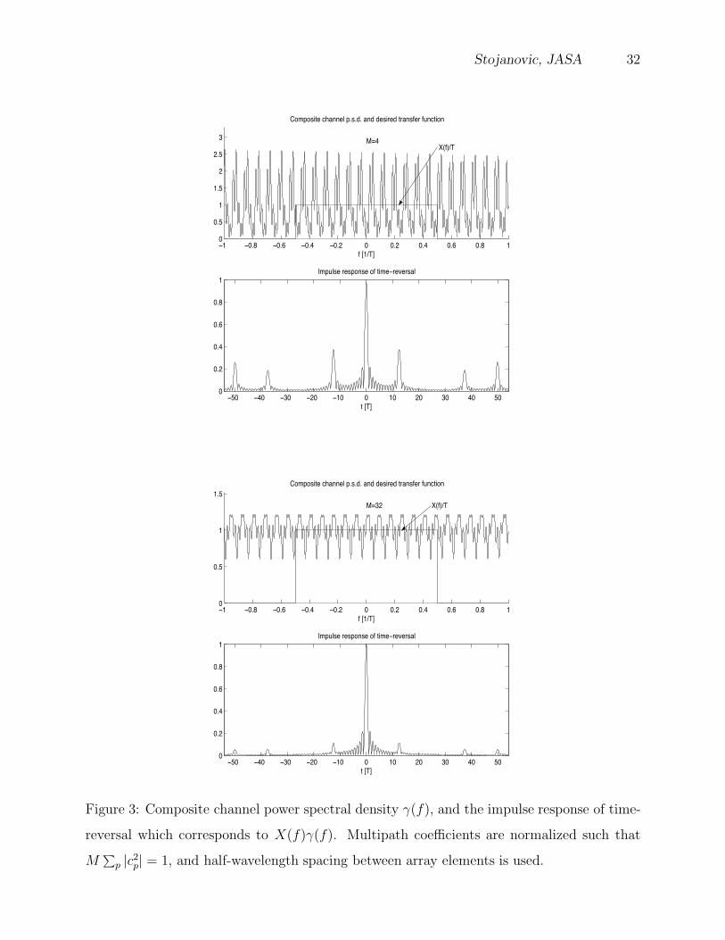
The channel function #(f) is shown in Fig. 3 for M = 4 and M = 32. Shown on the same

plot is the desired system response X(f) chosen as a raised cosine with roll-o" factor close to

0, which provides maximal bit rate for ISI-free transmission in a bandwidth B = 1/T . The

symbol duration is chosen to be T=0.2 ms, corresponding to the bandwidth of 5 kHz and

transmission at 10 kbps if 4-PSK is used, or 15 kbps if 8-PSK is used. The impulse response

of the overall system obtained with time-reversal is also shown, and it is evidently far from

ideal. As the number of array elements is increased, #(f) tends to flatten out, resulting in

better, but not complete suppression of multipath through time-reversal.

c)For fc in kHz, a(fc) is given in dB/km as 10 loga(fc) = 0.11f2c /(1 + f2

c ) + 44f2c /(4100 + f2

c ) + 2.75 ·

10!4f2c + 0.003.

Stojanovic, JASA 21

B. Performance analysis

Fig. 4 summarizes performance results for the two examples. Let us focus on the M = 4

case. We first confirm that two-sided focusing (Eq. 29, solid curve labeled ‘&’) outperforms

one-sided focusing (Eq. 30, dashed curve labeled ‘&’), but more interestingly, we observe

that the di"erence in performance is small. This is an encouraging observation from the

viewpoint of designing a practical system with restricted processing complexity. The per-

formance of time-reversal (Eq. 33, dashed curve) is inferior to optimal focusing and to all

other schemes at practical values of SNR. By practical, those values are meant that yield at

least several dB of output SNR, as this is required for an adaptive system to perform in a

decision-directed manner. The loss of time-reversal becomes quite large even at a moderate

E/N0 of 10 dB - 15 dB, and the performance saturates thereafter at a value 1/% determined

by the channel (34). Some of the loss is recovered by the use of an equalizer in conjunc-

tion with transmit time-reversal (Eq. 41, curve labeled ‘+’). However, it is interesting to

observe that this system compares poorly with the standard equalizer that uses square-root

raised cosine transmit filters and equal energy allocation across the array (Eq. 44, dashed

curve labeled ‘o’). Standard downlink equalization is inferior to its uplink counterpart (Eq.

46, solid curve labeled ‘o’ ), which o"ers a consistently good performance. Note that this

performance is closely matched by one-sided focusing at moderate to high SNR. Finally,

we confirm that equalization using optimized transmit filters (Eq. 67, curve labeled ‘*’)

provides an upper bound on the performance of all other schemes. More importantly, we

observe that this scheme o"ers negligible improvement over focusing, which allows a much

easier implementation.

With M = 32, the performance of time-reversal improves; however, the saturation e"ect

is still notable. Nonetheless, it has to be noted that at low and moderate E/N0 up to about

10 dB or 15 dB, with the increased number of elements, time-reversal becomes the tech-

nique of choice as it o"ers near-optimal performance at minimal computational complexity.

Equalization in conjunction with transmit time-reversal now outperforms standard downlink

equalization, while the performance of both focusing methods, as well as that of standard

uplink equalization, tends to the same optimal curve. Comparing the performance achieved

Stojanovic, JASA 22

with 32 and with 4 elements demonstrates that optimal focusing is much less sensitive to the

array size than either of the techniques based on time-reversal (recall also that the power in

the channel is kept constant with changing M).

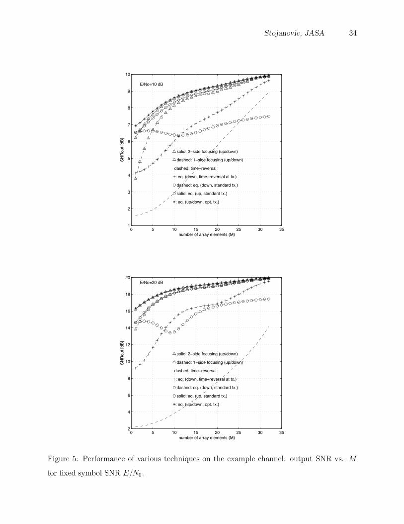
Performance sensitivity to the array size is summarized in Fig. 5 which shows the output

SNR as a function of M for a given symbol SNR E/N0. Two values of E/N0 are taken as

an example, 10 dB and 20 dB. In each instance, we note superiority of focusing methods

over time-reversal. Performance of focusing methods shows fast improvement with initial

increase in M , and a small increment thereafter. Hence, good performance can be achieved

without unduly increasing the number of array elements. For example, if one-sided focusing

is used, and E/N0 & 10 dB, increasing the number of elements beyond 6 o"ers less than 3 dB

total improvement in performance. In contrast to this situation, time-reversal steadily gains

in performance within the range of M shown; however, it fails to achieve the performance

of focusing methods. Most importantly, we observe that at moderate to high symbol SNR,

one-sided focusing needs a relatively small number of array elements to approach the optimal

performance.

Results of Fig. 5 also o"er an interesting comparison between standard equalization

and equalization in conjunction with transmit time-reversal. Using time-reversal at the

transmitter o"ers an improvement provided that M is greater than a certain number. In the

example considered, this number is 11 at E/N0 of 10 dB, and 8 at E/N0 of 20 dB.

So far, we have considered up to M = 32 elements, but it is interesting to observe

the performance of time-reversal with a further increase in M , to see what array size is

needed to bring its performance to that of other techniques. Fig. 6 shows the performance

of time-reversal for an extended range of M . Shown on the same plot is the performance

of optimal focusing, which, on this scale, is indistinguishable from the system bound or

multichannel equalization. An interesting e"ect is immediately apparent: the performance

of time-reversal does not consistently improve with increasing M (as does the performance

of focusing techniques and uplink equalization) but instead exhibits an oscillatory behavior,

tending to the optimum only as M $ (. The values of M for which the performance is best

are those values for which it happens so that the composite channel function #(f) flattens

out almost completely, i.e., #(f) + 1. At these values of M , time-reversal approaches the

Stojanovic, JASA 23

performance bound. However, due to the nature of the function #(f), the performance does

not remain at optimum, but deviates from it with an increase in M . This fact underlines

the suboptimality of system design based on time-reversal only. In practice, it could be

di!cult to rely on finding the optimal number of elements every time the array is deployed

and system configuration changes.

Finally, we investigate performance sensitivity to the changes in multipath composition

and the array element spacing, both of which influence the channel function #(f). Fig. 7

shows performance results obtained for the same channel model, but with six, instead of

three multipath components taken into account. The total multipath spread is now some-

what greater than 60 ms, with the additional arrivals’ strength approximately 9, 12, and 15

dB below the principal arrival. The performance di"ers little as compared to the three-path

channel. If anywhere, the di"erence can be seen when only a few elements are used–the per-

formance of time-reversal is then worse on the six-path channel, while that of other techniques

is better. More importantly, we observe that the same conclusions regarding performance

comparison between di"erent techniques hold in the presence of extended multipath. To

assess performance sensitivity to changes in relative strength of the multipath arrivals, a

hypothetical case of a lossless six-path channel was investigated. Su!ce it to say that the

same general conclusions were made in this case.

The e"ect of changing the array element spacing is illustrated in Fig. 8. This figure

shows performance results for the original three-path channel, but with d = 1.41&c instead

of d = &c/2. Evidently, the performance of time-reversal shows more sensitivity to the

changes in the array element spacing than the other techniques (the same would be true for

changes in the carrier frequency). The optimum is now approached with a smaller number of

elements (this number corresponds to the same total array length, i.e., 40 elements spaced by

&c/2 or 14 elements spaced by 1.41&c in the example considered). However, the improvement

in performance is not consistent with an increase in the element spacing. For a given number

of elements M > 1, performance improves with an initial increase in element spacing, but

exhibits an oscillatory behavior afterwards. For example, with M = 4, performance starts

to degrade after element spacing increases beyond 5 &c. With elements spaced by 10&c, at

E/N0=20 dB, the output SNR does not exceed a value of about 8 dB if more than two

Stojanovic, JASA 24

elements are used in a time-reversal array. Compared to this situation, performance of

retrofocusing techniques shows negligible sensitivity to the changes in element spacing.

IV. CONCLUSION

A number of techniques have been investigated for communication over an underwater

acoustic link where one end is equipped with a single transmit/receive element and another

with an array. To achieve maximal bit rate within a fixed bandwidth, an optimization

criterion of maximizing the data detection SNR, while eliminating or minimizing the residual

ISI was chosen. Transmit/receive filters were obtained analytically for uplink and downlink

transmission, with varying degrees of system complexity. The so-obtained optimal techniques

were compared to standard time-reversal and equalization.

Because it ignores residual ISI, time-reversal exhibits performance saturation, and strongly

depends on the use of a large array. When this can be a"orded (e.g. in a network whose base

station uses an array to isolate multiple users) time-reversal o"ers a solution for minimal-

complexity processing. With a smaller array, however, standard equalization outperforms

time-reversal, and the use of equalization in conjunction with transmit time-reversal does

not guarantee performance improvement over standard equalization, unless the number of

elements exceeds a certain value. The proposed method of spatio-temporal retrofocusing

guarantees maximal SNR and elimination of ISI for an arbitrary array size. It outperforms

time-reversal at the expense of additional filtering. The filters needed for optimal focusing

include phase-conjugation augmented by a channel-dependent scaling function. If filter ad-

justment is constrained to the array side only, one-sided focusing o"ers an excellent trade-o"

between complexity and performance. Its performance has only a small loss with respect to

the two-sided focusing, and it stays close to that of uplink multichannel equalization. It thus

represents a solution for systems that cannot deploy large arrays and have limited processing

power. In addition, when two-way communication is to be established over a white-noise

channel, the same set of filters can be used for transmission and reception.

The system analysis was completed by optimizing both ends of an equalization based

system. While it is unlikely that a practical system would be based on this approach due

Stojanovic, JASA 25

to the di!culty of finding optimal filters, it provides an upper bound on the performance of

all other techniques. Results demonstrate that optimal focusing performs very close to this

bound.

Future work will concentrate on an experimental validation of spatio-temporal focusing

aided by adaptive channel estimation. Two types of errors will guide the system performance:

the error due to noise and the error due to time-variability of the channel. In particular,

the latter may prove as the limiting factor for the performance of an acoustic system with a

long round-trip delay and high rate of channel variation. Future analytical work will address

system optimization with imperfect channel knowledge.

Stojanovic, JASA 26

REFERENCES

1 M.Stojanovic, J.Catipovic and J.Proakis, “Reduced-complexity multichannel process-

ing of underwater acoustic communication signals,” J. Acoust. Soc. Am., 98(2), Pt.1,

pp.961-972, Aug. 1995.

2 M.Fink, F.Wu, J.-L.Tomas and D.Cassereau, “Time-reversal of ultrasonic fields–Parts

I, II and III,” IEEE Trans. Ultrasonics, Ferroelectrics and Freq. Control,, vol.39, No.5,

Sept. 1992, pp. 555-592.

3 W.A.Kuperman, W.S.Hodgkiss, H.C.Song, T.Akal, C.Ferla and D.R.Jackson, “Phase

conjugation in the ocean: Experimental demonstration of an acoustic time-reversal

mirror,” J. Acoust. Soc. Am., 103(1), pp.25-40, Jan. 1998.

4 W.S.Hodgkiss, H.C.Song, W.A.Kuperman, T.Akal, C.Ferla and D.R.Jackson, “A long-

range and variable focus phase-conjugation experiment in shallow water,” J. Acoust.

Soc. Am., 105(3), pp.1597-1604, March 1999.

5 W.S.Hodgkiss, J.D.Skinner, G.E.Edmonds, R.A. Harriss and D.E.Ensberg, “A high

frequency phase-conjugation array,” in Proc. IEEE Oceans’01 Conference, pp.1581-

1585, Nov. 2001.

6 J.S.Kim, H.C.Song and W.A.Kuperman, “Adaptive time-reversal mirror,” J. Acoust.

Soc. Am., 109(5), pp.1817-1825, May 2001.

7 G.Edelmann, W.S.Hodgkiss, W.A.Kuperman and H.C.Song, “Underwater acoustic

communication using time-reversal,” in Proc. IEEE Oceans’01 Conference, Nov. 2001.

8 H.C.Song, G.Edelmann, S.Kim, W.S.Hodgkiss, W.A.Kuperman and T.Akal, “Low and

high frequency ocean acoustic phase conjugation experiments,” Proceedings of SPIE,

vol.4123 (2000), pp.104-108.

9 D.Jackson and D.Dowling, “Phase-conjugation in underwater acoustics,” J. Acoust.

Soc. Am., vol.89(1), pp.171-181, Jan. 1991.

Stojanovic, JASA 27

10 D.Rouse", D.R.Jackson, W.L.J.Fox, C.D.Jones, J.A.Ritcey and D.R.Dowling, “Under-

water acoustic communication by passive-phase-conjugation: Theory and experimental

results,” IEEE J. Oceanic Eng., vol.26, No.4, pp. 821-831, Oct. 2001.

11 D.Jackson, J.A.Ritcey, W.L.J.Fox, C.D.Jones, D.Rouse" and D.R.Dowling, “Experi-

mental testing of passive phase-conjugation for underwater acoustic communication,”

in Proc. 34th Asilomar Conference, pp.680-683, 2000.

12 J.Flynn, W.L.J.Fox, J.A.Ritcey, D.R.Jackson and D.Rouse", “Decision-directed pas-

sive phase-conjugation for underwater acoustic communications with results from a

shallow-water trial,” in Proc. 35th Asilomar Conference, pp.1420-1427, 2001.

13 D.Rouse", J.A.Flynn, W.L.J.Fox and J.A.Ritcey, “Decision-directed passive phase-

conjugation for underwater acoustic communication: experimental results,” in Proc.

IEEE Oceans’02 Conference, Oct. 2002.

14 J.A.Flynn, W.L.J.Fox, J.A.Ritcey and D.Rouse", “Performance of Reduced-

Complexity Multi-Channel Equalizers for Underwater Acoustic Communications,” in

Proc. 36th Asilomar Conference, vol.1, pp.453-460, 2002.

15 J.Gomes and V.Barroso, “The performance of sparse time-reversal mirrors in the con-

text of underwater communications,” in Proc. 10th IEEE Workshop on Statistical Sig-

nal and Array Processing, pp.727-731, 2000.

16 J.Gomes and V.Barroso, “A matched-field processing approach to underwater acoustic

communication,” in Proc. IEEE Oceans’99 Conference, pp.991-995, Sept. 1999.

17 J.Gomes and V.Barroso, “Asymmetric underwater acoustic communication using time-

reversal mirror,” in Proc. IEEE Oceans’01 Conference, Sept. 2000.

18 J.Gomes and V.Barroso, “Wavefront segmentation in phase-conjugate arrays for spa-

tially modulated acoustic communication,” in Proc. IEEE Oceans’01 Conference,

pp.2236-22434, Oct. 2001.

Stojanovic, JASA 28

19 J.Gomes and V.Barroso, “Ray-based analysis of a time-reversal mirror for underwater

acoustic communication,” in Proc. ICASSP’00 Conference, pp.2981-2984, 2000.

20 J.Gomes and V.Barroso, “Time-reversed communication over Doppler-spread under-

water channels,” in Proc. ICASSP’02 Conference, pp.2849-2852(III), 2002.

21 P.Hursky, M.Porter, J.Rice and V.McDonald, “Passive phase-conjugate signaling using

pulse-position modulation,” in Proc. IEEE Oceans’01 Conference, Nov. 2001.

22 T.C.Yang, “Temporal resolutions of time-reversal and passive phase-conjugation for

underwater acoustic communications,” IEEE J. Oceanic Eng., vol.28, No.2, pp. 229-

245, Apr. 2003.

23 J.SKim and K.C.Shin, “Multiple focusing with adaptive time-reversal mirror,” J.

Acoust. Soc. Am., 115(2), pp.600-606, Feb. 2004.

24 D.Gesbert, M.Shafi, D.Shiu, P.J.Smith and A.Naguib, ”From theory to practice: An

overview of MIMO space-time coded wireless systems,” IEEE J.Select. Areas Commun.,

vol.21, No.3, pp.281-302, Apr. 2003.

25 M.Stojanovic and Z.Zvonar, “Multichannel processing of broadband multiuser commu-

nication signals in shallow water acoustic channels,” IEEE J. Oceanic Eng., vol.21,

pp.156-166, Apr. 1996.

26 D.Kilfoyle, J.Preisig and A.Baggeroer, “Spatial modulation over partially coherent

multi-input / multi-output channels,” IEEE Trans. Sig. Proc., vol.51, No.3, pp.794-

804, March 2003.

27 J.G.Proakis, Digital Communications, New York: Mc-Graw Hill, 1995.

28 M.Stojanovic, “E!cient acoustic signal processing based on channel estimation for

high rate underwater information,” submitted to J.Acoust. Soc. Am. (available at

http://www.mit.edu/ millitsa/publications.html)

Stojanovic, JASA 29

List of Figures

1 Uplink (above) and downlink (below) transmission. An equalizer (dashed box)

may or may not be used. . . . . . . . . . . . . . . . . . . . . . . . . . . . . . 30

2 Multipath characteristics of the example channel: path gain magnitudes |cp|

and angles of arrival (p are shown at corresponding delays 'p (reference delay

is '0 = 0). . . . . . . . . . . . . . . . . . . . . . . . . . . . . . . . . . . . . . 31

3 Composite channel power spectral density #(f), and the impulse response

of time-reversal which corresponds to X(f)#(f). Multipath coe!cients are

normalized such that M&

p |c2p| = 1, and half-wavelength spacing between

array elements is used. . . . . . . . . . . . . . . . . . . . . . . . . . . . . . . 32

4 Performance of various techniques on the example channel: output SNR vs.

E/N0 for fixed number of array elements M . . . . . . . . . . . . . . . . . . . 33

5 Performance of various techniques on the example channel: output SNR vs.

M for fixed symbol SNR E/N0. . . . . . . . . . . . . . . . . . . . . . . . . . 34

6 Performance of time-reversal and optimal focusing for extended range of M. 35

7 Output SNR vs. M for the six-path channel model, d = &c/2. . . . . . . . . 36

8 Output SNR vs. M for the three-path channel model, d = 1.41&c. . . . . . 37

Stojanovic, JASA 30

d(n)

! G0(f) !

! C1(f) ! +

"

w1(t)

! G1(f) !

! CM (f) ! +

"

wM(t)

! GM (f) !

... ! ###

! A[f ] !d̂(n)y(n)

channel

!d(n)

! G1(f) ! C1(f) !

! GM (f) ! CM (f) !

... ! ! +

"

w0(t)

! G0(f) ###

!y(n)

A[f ] !d̂(n)

channel

Figure 1: Uplink (above) and downlink (below) transmission. An equalizer (dashed box)

may or may not be used.

Stojanovic, JASA 31

0 2 4 6 8 100

0.1

0.2

0.3

0.4

0.5

0.6

0.7

0.8

path delay [ms]

multipath properties

bars: multipath coefficients (normalized power)

circles: angles of arrival [pi rad]

Figure 2: Multipath characteristics of the example channel: path gain magnitudes |cp| and

angles of arrival (p are shown at corresponding delays 'p (reference delay is '0 = 0).

Stojanovic, JASA 32

!1 !0.8 !0.6 !0.4 !0.2 0 0.2 0.4 0.6 0.8 10

0.5

1

1.5

2

2.5

3M=4

Composite channel p.s.d. and desired transfer function

f [1/T]

!50 !40 !30 !20 !10 0 10 20 30 40 500

0.2

0.4

0.6

0.8

1

t [T]

Impulse response of time!reversal

X(f)/T

!1 !0.8 !0.6 !0.4 !0.2 0 0.2 0.4 0.6 0.8 10

0.5

1

1.5

M=32

Composite channel p.s.d. and desired transfer function

f [1/T]

!50 !40 !30 !20 !10 0 10 20 30 40 500

0.2

0.4

0.6

0.8

1

t [T]

Impulse response of time!reversal

X(f)/T

Figure 3: Composite channel power spectral density #(f), and the impulse response of time-

reversal which corresponds to X(f)#(f). Multipath coe!cients are normalized such that

M&

p |c2p| = 1, and half-wavelength spacing between array elements is used.

Stojanovic, JASA 33

!5 0 5 10 15 20 25 30 35!5

0

5

10

15

20

25

30

35

E/No [dB]

SN

Ro

ut

[dB

]

solid: 2!side focusing (up/down)

dashed: 1!side focusing (up/down)

dashed: time!reversal

: eq. (down, time!reversal at tx.)

dashed: eq. (down, standard tx.)

solid: eq. (up, standard tx.)

: eq. (up/down, opt. tx.)

M=4

!5 0 5 10 15 20 25 30 35!5

0

5

10

15

20

25

30

35

E/No [dB]

SN

Ro

ut

[dB

]

solid: 2!side focusing (up/down)

dashed: 1!side focusing (up/down)

dashed: time!reversal

: eq. (down, time!reversal at tx.)

dashed: eq. (down, standard tx.)

solid: eq. (up, standard tx.)

: eq. (up/down, opt. tx.)

M=32

Figure 4: Performance of various techniques on the example channel: output SNR vs. E/N0

for fixed number of array elements M .

Stojanovic, JASA 34

0 5 10 15 20 25 30 351

2

3

4

5

6

7

8

9

10

number of array elements (M)

SN

Ro

ut

[dB

]

solid: 2!side focusing (up/down)

dashed: 1!side focusing (up/down)

dashed: time!reversal

: eq. (down, time!reversal at tx.)

dashed: eq. (down, standard tx.)

solid: eq. (up, standard tx.)

: eq. (up/down, opt. tx.)

E/No=10 dB

0 5 10 15 20 25 30 352

4

6

8

10

12

14

16

18

20

number of array elements (M)

SN

Ro

ut

[dB

]

solid: 2!side focusing (up/down)

dashed: 1!side focusing (up/down)

dashed: time!reversal

: eq. (down, time!reversal at tx.)

dashed: eq. (down, standard tx.)

solid: eq. (up, standard tx.)

: eq. (up/down, opt. tx.)

E/No=20 dB

Figure 5: Performance of various techniques on the example channel: output SNR vs. M

for fixed symbol SNR E/N0.

Stojanovic, JASA 35

0 20 40 60 80 100 1200

5

10

15

20

25

30

number of array elements (M)

SN

Ro

ut

[dB

]

solid: focusing

dashed: time!reversal

E/No

30 dB

25 dB

20 dB

15 dB

10 dB

5 dB

Figure 6: Performance of time-reversal and optimal focusing for extended range of M.

Stojanovic, JASA 36

0 5 10 15 20 25 30 350

2

4

6

8

10

12

14

16

18

20

number of array elements (M)

SN

Ro

ut

[dB

]

solid: 2!side focusing (up/down)

dashed: 1!side focusing (up/down)

dashed: time!reversal

: eq. (down, time!reversal at tx.)

dashed: eq. (down, standard tx.)

solid: eq. (up, standard tx.)

: eq. (up/down, opt. tx.)

E/No=20 dB

Figure 7: Output SNR vs. M for the six-path channel model, d = &c/2.

Stojanovic, JASA 37

0 5 10 15 20 25 30 352

4

6

8

10

12

14

16

18

20

22

number of array elements (M)

SN

Ro

ut

[dB

]

solid: 2!side focusing (up/down)

dashed: 1!side focusing (up/down)

dashed: time!reversal

: eq. (down, time!reversal at tx.)

dashed: eq. (down, standard tx.)

solid: eq. (up, standard tx.)

: eq. (up/down, opt. tx.)

E/No=20 dB

Figure 8: Output SNR vs. M for the three-path channel model, d = 1.41&c.