quotation from it or information derived from it is to be ... simulations software: commsim ... d.1...
TRANSCRIPT

The copyright of this thesis vests in the author. No quotation from it or information derived from it is to be published without full acknowledgement of the source. The thesis is to be used for private study or non-commercial research purposes only.
Published by the University of Cape Town (UCT) in terms of the non-exclusive license granted to UCT by the author.
Univers
ity of
Cap
e Tow
n

Decoding Algorithms for Continuous Phase Modulation
Werner Frederick Kleyn
4th June 2002
Univers
ity of
Cap
e Tow
n

2
Acknowledgements
I would like to thank Professor Robin Braun for bis supervision of this research as well as the
Department of Electrical Engineering at the University of Cape Town. Also thank you to Dr Daniel
Mashao who acted as internal supervisor during the latter stage of this research.
Tellumat Pty (Ltd) provided financial assistance for which I am very grateful.
There were times when I had to neglect my family and friends in order to complete this research.
Thank you for your patience and encouragement.
Finally, I wish to thank the LORD for His grace and the encouragement I received from Him
without I would not have been able to complete this research.
Univers
ity of
Cap
e Tow
n
Contents
1 Introduction
1.1 Background
10
10
1.2 Problem definition and Motivation 11
1.3 Objectives and Method ...... 12
2 System. description 13
2.1 Introduction.................................... 13
2.2 Traditional Description of the Continuous Phase Modulated (CPM) signal. 13
2.3 Tilted Phase Description of the CPM signal 14
2.4 Description of the 4-ary CPFSK signal. . . . . . . 14
2.5 Maximum Likelihood Receivers . . . . . . . . . . . 15
2.5.1 Maximum Likelihood Sequence Estimation
2.5.2 The Viterbi Algorithm (VA)
2.5.3 Obtaining the branch metrics
2.5.4 Implementation of the VA ..
2.6 Bit error rate performance . . . . . .
2.6.1 Bit error rate (BER) simulation.
3 Sequential Decoding Algorithm.s
3.1 Sequential Decoding
3.2 The Fano algorithm ...... .
3.2.1 Simulations ....... .
3.3 Performance Analysis and Summary
4 Neural Network-based Receivers
4.1 Introduction ........... .
4.1.1 The Single Layer Perceptron ..
4.1.2 Specification of Neural Networks
4.1.3 Conventional Pattern Recognition versus Trellis Decoding
4.1.4 Neural Network Receiver ..
4.1.5 Training of Neural Networks ............. .
4.1.6 A simple case: FFSK ................. .
4.2 Neural Network Decoding applied to MSK and 4-ary CPFSK
4.2.1 Sensitivity Analysis ........ .
4.2.2 Performance Analysis and Summary
4.2.3 Complexity..............
5
15
17 18
20
22
25
28
28
30
36
38
48
48 48
49 50
51
51
52
52
56
61
64
Univers
ity of
Cap
e Tow
n

CONTENTS
5 Conclusion
5.1 Summary ............ .
5.1.1 The FallO Algorithm .. . 5.1.2 The Neural Net Decoder.
5.2 Future Work .......... .
A The Back-propagation Neural Net Training Algorithm
B Perceptron Convergence Procedure for FSK
C Sensitivity Matrix for 16-4-4 NN MSK
C.1 Sensitivity matrix for training set 5To.5
C.2 Sensitivity matrix for training set 3Tl.O
D Simulations Software: Commsim
D.1 Functions . . . . . . . . . . . . . . . . . . . . . ..
D.2 Function Instance Initialization and Data Storage.
D.3 Handling of System Time and Clock . . . . . . . .
6
65
65
65
66
66
61
69
10 70 73
16
76
76 77
Univers
ity of
Cap
e Tow
n

List of Figures
2.1 Phase tree for 4-ary CPFSK over the first two intervals
2.2 State trellis for 4-ary CPFSK . . . . . . . .
2.3 Root to Toor State trellis for 4-ary CPFSK . .
2.4 Circuit for generating branch metrics . . . . . .
2.5 Simplified circuit for generating branch metric.
2.6 4-ary CPFSK baseband signals ........ .
2.7 8i(t) and 8k(t) in signal space .......... .
15
16
18
19
21
21
22
2.8 A few minimum distance error events for 4-ary CPFSK 24
2.9 BER results for MSK and FSK . . . . . . . . 26
2.10 BER results for 4-ary CPFSK, Tstep = T s /40 . . . . . . 27
3.1 Typical plot of d(l) showing incorrect decision at interval 1 29
3.2 The basic Fano Algorithm . . . . . . . . . . . . . . . . . . . 31
3.3 Received sequence for Example 1 and 2.a .......... 32
3.4 Received distance tree for Example 1 ((P - v) = 0.3, and ~ = 0.3) 33
3.5 Received distance tree for Example 2.a ((P - v) = 0.20, and ~ = 0.20) 33
3.6 Received sequence for Example 2.b and 3 ... . . . . . . . . . . . . . 34
3.7 Received distance tree for Example 2.b ((P - v) = 0.20, and ~ = 0.20) 34
3.8 Diagrams used for determination of optimum (p - v) and ~ma", . . . 35
3.9 Relationship among ~, (p - v) and l. . . . . . . . . . . . . . . . . . . . 36
3.10 Received distance tree for Example 3 ((p - v) = 0.12 and ~ = 0.18) . 37
3.11 Effect of ~ and (p - v) on Pe and number of backward steps, Eb/No = 16.00 dB 38
3.12 Distribution of instantaneous and maximum backward steps for Eb/No = 16.00 dB 39
3.13 Distribution of look-backs for Eb/No = 16.00 dB ................... 39
3.14 Distribution of instantaneous and maximum backward steps for Eb/No = 14.44 dB 40
3.15 Effect of ~ and (p - v) on Pe and number of backward steps, Eb/No = 13.10 dB. 41
3.16 Distribution of instantaneous and maximum backward steps for Eb/No = 13.10 dB 41
3.17 Distribution of look-backs for Eb/ No = 13.10 dB ................... 42
3.18 Effect of ~ and (p - v) on Pe and number of backward steps, Eb/No = 11.94 dB. 42
3.19 Distribution of instantaneous and maximum backward steps for Eb/No = 11.94 dB 43
3.20 Effect of ~ and (p - v) on Pe and number of backward steps, Eb/No = 10.00 dB. 43
3.21 Distribution of instantaneous and maximum backward steps for Eb/No = 10.00 dB 44
3.22 Effect of ~ and (p - v) on Pe and number of backward steps, Eb/No = 8.42 dB .. 44
3.23 Distribution of instantaneous and maximum backward steps for Eb/No = 8.42 dB . 45
3.24 Distribution of look-backs for Eb/No = 8.42 dB . . . . . . . . 45
3.25 Fano decoder DER performance. . . . . . . . . . . . . . . . . 46
3.26 Move-backs and look-backs as percentage of symbols received 46
7
Univers
ity of
Cap
e Tow
n

LIST OF FIGURES 8
4.1 Model of the Neuron 49
4.2 The sigmoid squashing function 50
4.3 Perceptron BER results for FFSK 53 4,4 8-4-4 Feedforward Network for MSK 54
4.5 Neural Network MSK Receiver . . . 54
4.6 BER results for MSK using 8-4-4 Neural Network. 55
4.7 Fully Connected 16-4-4 Feedforward Network for MSK (not all connections shown) 56
4.8 Demodulator structure . . . . . . . . . . . . . . . . . . . . . . . . . . . . . . . . .. 56
4.9 Best and worst BER results for MSK using 16-4-4 Neural Net. . . . . . . . . . .. 57
4.10 Maximum Sensitivity Numbers, MSE and corresponding number of bit errorS at
Eb/No of 10,45 dB, 16-4-4 NN. . . . . . . . . . . . . . . . . . . . . . . . . . . . .. 58
4.11 BER results for MSK using 16-8-4 Neural Net. . . . . . . . . . . . . . . . . . . .. 59
4.12 Maximum Sensitivity Numbers, MSE and corresponding number of bit errors at
Eb/No of 10,45 dB, 16-8-4 NN . . . . . . . . . . 60
4.13 Best and worst BER results for 4-ary CPFSK 63
D.1 Function data storage . . . . . . . . . . . . . . 77
Univers
ity of
Cap
e Tow
n

List of Tables
2.1 Pe equations for various modulation schemes .. 26
3.1 Set of Best Metrics as seen from "incorrect" state 29
3.2 Normalized metrics for 4-ary CPFSK, Es 0.5 J and Ts = 1 second. 30
3.3 Tree search for Example 1 «p - v) 0.3, and 6. = 0.3) . 32
3.4 Tree search for Example 2.a «p - v) = 0.2, and 6. = 0.2) 33
3.5 Tree search for Example 2.b «p v) = 0.2, and 6. = 0.2) 34
3.6 Tree search for Example 3 «P - v) 0.12, and 6. = 0.18) 36
3.7 Number of attempts to move back deeper than 12 symbol intervals for 6. = 0.06 47
3.8 Effect of the increase of (p - v), 6. constant . . . . . . . . . . . . . . . . . . . . .. 47
4.1 Training parameters (unless otherwise stated) used for MSK and 4-ary CPFSK
decoding . . . . . . . . . . . . . . . . . . . . . . . 52
4.2 Exemplars for MSK training, experiment 1 ... 53
4.3 MSE numbers for MSK, 16-4-4 Neural Network 54
4.4 16-4-4 Neural Network MSK Bit Errors ..... 55
4.5 16-4-4 Neural Network MSK Bit Errors ..... 55
4.6 Maximum sensitivity numbers parameters for 16-4-4 Neural Net for MSK 57
4.7 MSE and maximum sensitivity numbers for MSK, 16-8-4 Neural Network 58
4.8 16-8-4 Neural Network MSK Bit Errors ................... 59
4.9 16-8-8 Neural Network for MSK showing MSE, training cycles and maximum sensi-
tivity numbers ...................................... 60
4.10 16-8-8 Neural Network MSK Bit Errors ........................ 60
4.11 16-16-8 Neural Network for MSK showing MSE, training cycles and maximum sen-
sitivity numbers. . . . . . . . . . . . . . . . . . . . . . . . . . . .
4.12 16-16-8 Neural Network MSK Bit Errors ............. .
4.13 Exemplars for 4-ary CPFSK training (only class A shown here) .
4.14 16-16-8 Neural Network for 4-ary CPFSK, MSE .
4.15 16-16-8 Neural Network 4-ary CPFSK Bit Errors
4.16 16-16-8 Neural Network 4-ary CPFSK Bit Errors .
4.17 16-16-8 Neural Network 4-anJ CPFSK Bit Errors .
D.1 Modulator functions ..
D.2 Decoder functions ...
D.3 Demodulator functions.
D.4 Miscellaneous functions
9
61
61
62
62
62
62
62
76
76
76
77
Univers
ity of
Cap
e Tow
n
Chapter 1
Introduction
1.1 Background
Continuous Phase Modulation (CPM) possesses characteristics that make it very attractive for
many applications. Efficient non-linear power amplifiers can be used in the transmitters of constant
envelope CPM schemes. CPM also allows for the use of simple limiters in the demodulator rather
than linear receivers with gain controL These characteristics not only increases the life of the power source, but it improves circuit reliability since less heat is generated. In some applications,
such as satellite transmitters, where power and circuit failure is very expensive, CPM is the most
attractive choice. Bandwidth efficiency, also, is very attractive, and improves as the order of the scheme increases
(together with reduction in modulation index). Still further improvement is obtained through pulse
shaping which normally result in partial response schemes as opposed to full-response (CPFSK)
schemes.
The inherent memory or coding gain of CPM increases the minimum distance, which is a figure
of merit for a scheme's error performance. The length of the inherent memory is the constraint length of the scheme. Successful extraction of this inherent memory result in improved power
efficiency. By periodic variation of the modulation index as in multi-h CPFSK, a sub class of
CPM, coding gain or inherent memory can be significantly improved.
CPM demodulation is also less sensitive to fading channels than some other comparable systems.
Well-known schemes such as GSM digital mobile systems, DECT and Iridium all use some form of CPM to transport their information. These implementations are normally pulse-shaped FSK
or MSK and are used for the reasons above, except that their receivers do not always exploit the
inherent memory.
Unfortunately, though, when one wants to exploit the inherent memory of higher level CPM
schemes, all these attractive characteristics are offset by the complexity of the receiver structures
which increases exponentially in complexity as the order or constraint length is increased.
Optimum receivers for binary CPFSK were first described by Osborne and Luntz [19] in 1974 and their research was later extended by Schonhoff [26] to include M-ary CPFSK. These receivers evaluate likelihood functions after observing the received signal for a certain number of symbol
intervals, say N, then calculate a set of likelihood parameters on which a likelihood ratio test regarding the first symbol is based. These receivers are complex and impractical but does provide valuable insight. This is called maximum likelihood sequence estimation (MLSE).
Another way to do MLSE would be to correlate all possible transmitted sequences (reference signals at the demodulator) over a period of N symbol intervals with the received sequence. The
10
Univers
ity of
Cap
e Tow
n
CHAPTER 1. INTRODUCTION 11
first symbol of the reference sequence with which the received sequence has the largest correlation,
is decoded as the most likely symbol. The number of reference sequences required at the receiver
grow very fast as the observation period increases. Up to now, only the lowest order CPM schemes
have feasible optimal receiver structures.
The only practical solution thus far for the MLSE of higher order schemes is the use of soft
ware implementations of which the Viterbi algorithm is the most popular. Through recursive
or sequential processing of data per interval, the number of matched filters required can be re
duced. However, for schemes beyond a certain order and constraint length, the Viterbi algorithm's
consumption of computational resources reduces it's feasibility.
Research into CPM is focused mainly on the quest for simpler demodulators and decoders or
lower order schemes with better coding gain. In order to gain further insight into CPM, research
is approached from different angles.
Most significantly, in 1980 Massey [16] proposed a simple and practical MSK maximum likeli
hood demodulator. His starting point was to separate the continuous-phase coding/decoding and
memoryless modulation/demodulation functions of the MSK receiver/transmitter and later [17]
recommended that this principle should be extended to CPM schemes in general. Rimoldi [21] was
the first to present a generalized method of separating the continuous-phase coding and memory
less modulation functions of a CPM modulator. This decomposition approach has two important
implications. The memoryless modulator may be cascaded with the channel and a memory less
demodulator (a demodulator operating over one symbol interval) to form a discrete memoryless
channel. This channel can then be studied with well-established theory. The second implication is
that the continuous-phase encoder can be studied separately as a time-invariant linear sequential
circuit, using the same theory as that developed for convolutional encoders. This encoder can be
combined with an outside convolutional encoder to increase the minimum distance of the overall
scheme, while ensuring that the continuous-phase requirement of the transmitted waveform is met.
Schoonees [27] did a likelihood ratio analysis of CPFSK. In his research he analyzed Massey's
MSK receiver, based on the maximum likelihood receiver of Schonhoff [26], and discovered that
the likelihood ratio test of MSK simplify to the same decoder as proposed by Massey [16]. He then
extended this analysis to higher order CPFSK schemes and found that a similar simplification does
not exist for schemes other than MSK. The conclusion is that no simplified optimum receivers exist
for higher order CPFSK schemes.
Various reduced complexity decoders have been suggested. Reduced State Trellis decoding [8,
12, 30] is a method that tries to apply the Viterbi algorithm on the most promising part of the
demodulator output.
Recently, some research has been done on the feasibility of using neural networks as decoders [18,
32] for CPM. Poor results were obtained as the error performance seems to be very sensitive to
noise. The performance of these kinds of decoders are suboptimal, the architecture complex, but
it is believed that a neural net-based implementation will become practical as VLSI digital and/or
analogue neural network chips become feasible components.
1.2 Problem definition and Motivation
Power and bandwidth efficient CPM modulation schemes are well-defined, but feasible optimum
decoders l for these schemes does not exist [27], except for MSK.
The complexity of software decoders have become more manageable in recent years with the
advent of powerful digital signal processing integrated circuits. However, system cost is still largely
implementation that process the information received from the "memory less" demodulator.
Univers
ity of
Cap
e Tow
n

CHAPTER 1. INTRODUCTION 12
determined by complexity. The quest will always be for simplicity, which will lead to better power
efficiency, cost effectiveness and ease of implementation. So any research that lead to more insight
into CPM decoding, and performance results for possible simpler decoders, will be of value.
The use of neural networks implementations in decoding CPM has not been fully researched,
especially its behavior in the presence of noise. The Fano algorithm is a sequential decoding
algorithm of which the performance, when applied to CPM, is relatively unknown. Rimoldi [21]
showed that MSK can be decoded optimally with only one symbol delay. Applying his method
shows that 4-ary CPFSK need more than one symbol delay to be decoded optimally. This is
contradictory to intuition when studying 4-ary CPFSK state trellis and will need investigation
before comparing the results of any new algorithm with the optimum one. In summary then:
1. Neural network decoders seems to be very sensitive to Gaussian noise, leading to poor error
performance. Investigate this sensitivity and compare Neural Net-based decoder with an
optimum decoder.
2. Investigate the performance of the Fano algorithm as a decoder of CPM.
3. Investigate the optimum observation periods for CPFSK.
1.3 Objectives and Method
Most of this research is based on 4-ary CPFSK and MSK with the emphasis on effective software
decoding algorithms for 4-ary CPFSK.
Since error performance is an important figure of merit, we will establish a reliable error bound
for 4-ary CPFSK against which we can compare other decoders. The first objective will be to
conduct a search for optimum Fano algorithm parameters, that is, parameters that will minimize
error events and catastrophic failure.
Up to now, research on neural network trellis decoding was applied to higher level CPM schemes.
We will compare the performance of Viterbi-decoded 4-ary CPFSK and MSK with those of a Neural
Net-based ones. In this research I will assume white Gaussian noise as the only channel perturbation, that is, no
fading and band-limiting etc. Simulations will be performed using a custom written C program.
Univers
ity of
Cap
e Tow
n
Chapter 2
System descriptioll
2.1 Introduction
In this chapter we establish a baseline against which we will interpret the results of Chapters 3 and
4. The continuous phase modulated signal is described, as well as maximum likelihood sequence
estimation and the implementation of the Viterbi algorithm. Through simulation and mathematical
analysis we establish the bit error probability and the optimum observation window for decoding
4-ary CPFSK.
2.2 Traditional Description of the Continuous Phase Modu
lated (CPM) signal
The CPM signal is described by 12, 3]
set, a) = J2~. cos [27r/ot + <pet, a) + <Pol, (2.1)
where the information-carrying phase is
00
<pet, a) 21rh E ad(t - iT.), (2.2) .=0
The parameter T. is the channel-symbol time, E8 the energy per symbol, and h is the modu
lation index. The modulation index h determines the rate of change of the phase and is assumed
to be a rational number
(2.3)
where K and P are relative prime positive integers. This constraint gives the CPM system
a periodic (modulo-27r) phase structure, that is, a finite number of phase states, otherwise the
optimum receiver has infinite complexity.
I(t) = lot g(r)d(r) (2.4)
is the phase response function with get) a frequency shape function defined over a finite time
interval 0 :5 t :5 LT. and zero outside.
L is the length of the pulse, and is equal to the number of input symbols which affect the
13
Univers
ity of
Cap
e Tow
n

CHAPTER 2. SYSTEM DESCRlPTION 14
change in phase over the current symbol interval and is also sometimes called the memory of the
scheme. g(t) is defined to limit f(t) as follows:
f(t) = { ~' 2 ,
t<O
t;::: LTs (2.5)
Systems with L = 1 are called full-response schemes; whereas partial-response schemes have
L>1.
The M-ary information sequence is a (ao, all a2, a3, ... ) where
{ {±1, ±3, ... , ±(M -1)}
a'E • {O, ±2, ±4, ... , ± (M 1)}
M even, i;::: ° M odd, i';::: °
2.3 Tilted Phase Description of the CPM signal
The continuous phase modulated signal waveform can also be described [21] by
s(t, u) = J2~8 cos [211" Itt + 1/J(t, u) + <Po] , t;:::o
where 1/J(t, u) is the information-carrying phase defined as
00
1/J(t, u) = 411"h L ud(t - iTs), t;:::O ;=0
(2.6)
(2.7)
and It is an asymmetrical carrier frequency. The parameter u signifies a baseband data symbol
sequence u = (uo, 'Ul, U2, ... ) with Ui a member of the M-element alphabet {a, 1, ... , (M 1)}.
Rimoldi [21] translated the traditional phase <p(t, a) and symmetrical carrier frequency fa of Equa
tion 2.2 into the tilted phase and asymmetrical carrier frequency as it appear in Equation 2.6. This
allowed him to decompose the CPM modulator into a continuous-phase encoder (CPE) and a mem
oryless modulator (MM). We will use the tilted phase description of the CPM signal throughout
this research.
2.4 Description of the 4-ary CPFSK signal
Continuous-Phase Frequency-Shift-Keying (CPFSK) is a full-response L = 1 CPM scheme charac
terized by the phase response function
f(t) = {
0,
1 2
(2.8)
For (M = 4)-ary CPFSK, h = 1/4. We can now plot the information carrying phase 1/J(t, u)
versus time for all possible symbol sequences. This phase tree (<po = 0) is illustrated in Figure 2.1
and the corresponding state trellis in Figure 2.2. On the state trellis, each state er is associated
with a phase state on the phase tree, taken modulo-211". From the state trellis it can be seen that
there is a one-to-one correspondence between the information sequence u and the state sequence
er, as described by the following equation:
'Un (ern+! - ern) mod(M) (2.9)
Univers
ity of
Cap
e Tow
n

CHAPTER 2. SYSTEM DESCRIPTION 15
where "mod" is the modulo operator. A signal set, un) transmitted during the n-th signalling
interval is represented on the state trellis by the vector Xn (un, Un).
1/!(t, Un)
121l'h
T 2T
Figure 2.1: Phase tree for 4-ary CPFSK over the first two intervals
2.5 Maximum Likelihood Receivers
2.5.1 Maximum Likelihood Sequence Estimation
The following paragraphs are along the lines of [1]. The function of a maximum likelihood detector
is to choose that valid signal vector that was most likely to have been transmitted given the received
channel output vector. This corresponds to finding that allowable signal vector SI that maximizes
the log-likelihood function
(2.10)
where r is the received channel output vector that includes noise. It does not require a pri
ori information about the parameter of interest. If the transmit signal vector alphabet contains
elements that are a priori equally probable, this decision rule can mathematically be reduced to
minimization of the function Ilr - Sill with respect to i. The term Ilr - Si II is the distance in vector space between the two vectors ( norm), also called the
Euclidean distance. This shows that the maximum-likelihood decision rule estimates the received
signal vector to be that one which is closest in Euclidean distance to one of the element vectors
in the transmit signal vector alphabet. Similarly, the function of a maximum likelihood sequence
estimator is to find that allowable signal sequence that was most likely to have been transmitted
given the received channel output signal. This is equivalent to finding that "allowable" transmitted
Univers
ity of
Cap
e Tow
n

CHAPTER 2. SYSTEM DESCRIPTION 16
(0,3)
2 (rr)
o (0) n 2 n 1 n n+l
Figure 2.2: State trellis for 4-ary CPFSK
signal sequence s(t, u) that maximizes the log-likelihood function
In [Pr(r(t)/s(t, u))] (2.11)
where r(t) is the received channel output, r(t) == s(t, u) + n(t), and the noise n(t) is Gaussian
and white. The parameter u signifies a baseband input symbol sequence, where each symbol
has length Ts and is selected from a fixed alphabet. In the case of continuous phase modulation
(CPM), this baseband signal is used to modulate the phase of some carrier frequency, resulting in
the sequence s(t, u), as shown previously. Again, this decision rule can be reduced to minimization
of the squared Euclidean distance function
Ilr(t) - s(t, u)112 (2.12)
In the normed vector space, Parseval's identity can be used to show that:
Ilr(t) s(t, u)112 / [r(t) - s(t, U)]2 dt (2.13)
Expanding the right side of this equation shows that minimization of this Euclidean distance
function is equivalent to maximizing the correlation
(NT, J(u) J
o r(t)s(t, u) dt (2.14)
where the source sequence u consists of N symbols. The value of this integral is the metric
used by the maximum likelihood receiver to decide the likelihood that a particular signal was sent.
In principle, our maximum likelihood sequence estimator is a correlation receiver, in which all
Univers
ity of
Cap
e Tow
n

CHAPTER 2. SYSTEM DESCRIPTION 17
possible transmitted signals 8(t, u) (reference signals) are correlated with the received signal. The
reference signal8(t, u) that result in the largest correlation with the received signal r(t) is chosen
as the transmitted signaL The symbol sequence u corresponding to this most likely transmitted
signal is obviously our decoded symbol sequence. The number of reference signals 8(t, u) required
at the receiver grow very fast as the observation period NTe increases. There are MNpossibilities,
where M = 4 for 4-ary CPFSK. For example, with M = 4 and N 100, one would have to
perform 4100 correlations! This is not a feasible structure in practice.
Our problem is analogous to finding the shortest (or longest) route between two nodes, with
many randomly distributed nodes in between. The Viterbi algorithm is a recursive procedure that
was developed to solve this type of problem. Applied to our problem, it finds that sequence which
maximizes the log-likelihood function (the metriC) up to the nth symbol intervaL
2.5.2 The Viterbi Algorithm (VA)
The Viterbi algorithm (VA) [10] is a maximum-likelihood decoder. We can define the metric in
Equation 2.14 over the first n intervals of a given source sequence u as:
rNT, >'n(UO, ... , Un-I) 10 r(t)8(t, u) dt (2.15)
Since there is a one-to-one correspondence between the information sequence u and the state
sequence CT as mentioned earlier in that Un-l CTn - CTn-l, we can rewrite the last equation as
r T•
>'n(CTO, •.. , CTn ) 10 s(t, u)r(t) dt (2.16)
>'n(CTO, ... ,CTn ) can be computed recursively: By replacing n with n + 1 in Equation 2.16 we
obtain
r(n+l)T. >'n+l (CTO' •.. ,O"n+d = 10 s(t, u)r(t) dt
lnT• l(n+l)T.
8(t, u)r(t)dt + 8(t, u)r(t)dt ° nT.
= An(o,O, .... , Un) + AA(Xn)
where
1 (n+l)T.
a>'n(Xn) = s(t, u)r(t) dt nT.
(2.17)
(2.18)
(2.19)
(2.20)
Using this recursive approach, the receiver must now, in the n-th interval, computes a>'n(Xn)
for all ML P possible values of Xn and put the result in the state trellis, next to the applicable
branch. a>'n(Xn) = a>'n(Un , O"n) will be called a branch metric.
One way to find the sequence with the largest metric is to add the branch metrics along each
possible path in the trellis. However, this would still require us to compute MN branch metrics.
The number of calculations can be dramatically decreased by using the following observation
which is basic to the VA:
For any state at any specified depth in the trellis, the path with the highest overall metric (from
rootl to toor2 ) among all paths visiting that node accumulates also the highest metric between the
leftmost state in the state trellis is called the root zThe rightmost state in the state trellis is called the toor (notation used by [22])
Univers
ity of
Cap
e Tow
n
CHAPTER 2. SYSTEM DESCRIPTION
state U
3
2 •
root
o o
• • •
• • • 2 n- 2 n-l n
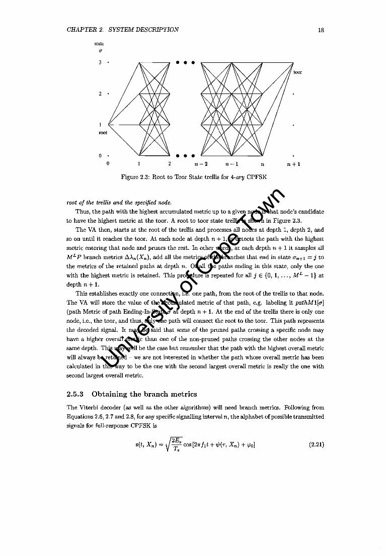
Figure 2.3: Root to Toor State trellis for 4-ary CPFSK
root of the trellis and the specified node.
18
toor
n+l
Thus, the path with the highest accumulated metric up to a given node is that node's candidate
to have the highest metric at the toor. A root to toor state trellis is shown in Figure 2.3.
The VA then, starts at the root of the trellis and processes all nodes at depth 1, depth 2, and
so on until it reaches the toor. At each node at depth n + 1, it detects the path with the highest
metric entering that node and prunes the rest. In other words, at each depth n + 1 it samples all
ML P branch metrics ~An(Xn), add all the metrics of the branches that end in state Un+l = j to
the metrics of the retained paths at depth n. Of all the paths ending in this state, only the one
with the highest metric is retained. This procedure is repeated for all j E {a, 1, ... , ML -I} at
depth n + 1.
This establishes exactly one connection, i.e. one path, from the root of the trellis to that node.
The VA will store the value of the accumulated metric of that path, e.g. labeling it pathM1[u]
(path Metric of path Ending-In-State U at depth n + 1. At the end of the trellis there is only one
node, Le., the toor, and thus, only one path will connect the root to the toor. This path represents
the decoded signal. It may be said that some of the pruned paths crossing a specific node may
have a higher overall metric than one of the non-pruned paths crossing the other nodes at the
same depth. This may well be the case but remember that the path with the highest overall metric
will always be retained - we are not interested in whether the path whose overall metric has been
calculated in this way to be the one with the second largest overall metric is really the one with
second largest overall metric.
2.5.3 Obtaining the branch metrics
The Viterbi decoder (as well as the other algorithms) will need branch metrics. Following from
Equations 2.6, 2.7 and 2.8, for any specific signalling interval n, the alphabet of possible transmitted
signals for full-response CPFSK is
(2.21)
Univers
ity of
Cap
e Tow
n
CHAPTER 2. SYSTEM DESCRIPTION
r(t) I(t, Un)
Inside Viterbi Processor
I L ___________________ ~
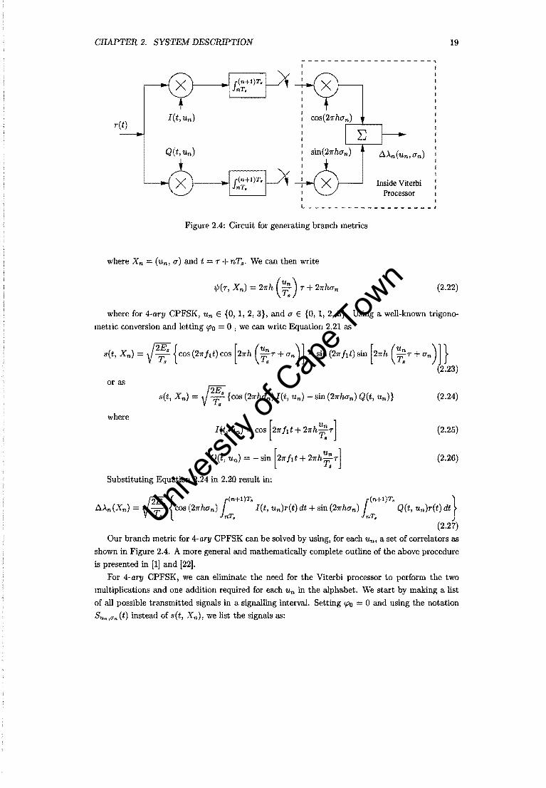
Figure 2.4: Circuit for generating branch metrics
where Xn = (un' a) and t = T + nTs. We can then write
19
(2.22)
where for 4-ary CPFSK, Un E {O, 1, 2, 3}, and a E {O, 1, 2, 3}. Using a well-known trigono
metric conversion and letting !Po 0, we can write Equation 2.21 as
or as
where
I(t, un) = cos [21rJtt+ 21rh~:T]
Q(t, Un) = -sin [21rftt+21rh~:T] Substituting Equation 2.24 in 2.20 result in:
(2.24)
(2.25)
(2.26)
f?E {l(n+l)T. l(n+l)T'} aAn(Xn) = T 8 cos (21rMn) J(t, un}r(t) dt + sin (21rMn) Q(t, un)r(t) dt
8 nT. nT.
(2.27)
Our branch metric for 4-ary CPFSK can be solved by using, for each Un, a set of correlators as
shown in Figure 2.4. A more general and mathematically complete outline of the above procedure
is presented in [1] and [22].
For 4-ary CPFSK, we can eliminate the need for the Viterbi processor to perform the two
multiplications and one addition required for each Un in the alphabet. We start by making a list
of all possible transmitted signals in a signalling interval. Setting !Po 0 and using the notation
SUn ,Un (t) instead of s(t, X n ), we list the signals as:
Univers
ity of
Cap
e Tow
n

CHAPTER 2. SYSTEM DESCRIPTION
We notice that
Signal Signal//w: T.
So,o(t): Re {e-iOe-i21rftt}
SI,O(t) : RT"'*' .."", l S2,O(t) : Re ei21rh ..f;r e-i21Tftt
Sa,o(t) : Re ei21rh -/,;r e-i21Tftt
SO,l(t): Re{e-i i e-i21r/l t }
Sl,l (t): Be r"( *,.,) ,,,, '" l
S2,1(t): Re ei21Th(..f;r+l)e-i21Tj,t
S3,1(t): Re ei21rh(i-r+1)e-i211"/lt
SO,2(t): Re { e-i1T e-i21f j,t} Sl,2(t): Re ,,;'"( *,H),,;','" l S2,2(t): Re ei21rh( ..f;r+2)e-i211"ltt
S3,2(t): Re ei21fh( -/,;r+2)e-i21r /tt
SO,3(t): Re e-i:lfe-i21f/l t }
S1,3 (t): Re J,.h( *'+')";"'" l S2,a(t): Re ei21rh( ..f;r+3) e-i211"/tt
S3,3(t): Re ei27rh( ..f;r+3)e-i:I1,./tt
So,o(t) == -SO,2(t)
Sl,O(t) == -Sl,2(t)
S2,O(t) -S2,2(t) Sg,o(t) = -Sa,2(t)
SO,l (t) -SO,3(t)
Sl,l (t) == -Sl,3(t)
S2,1 (t) == -S2,S(t) Sa,l (t) -Sa,a(t)
and consequently that
LUn(O, 0) -6.An(O, 2)
6.An(l, 0) = -6.An(l, 2)
6.An(2,0) == -6.An(2, 2)
6.An(3, 0) = -6.An(3, 2)
6.An(O, 1) == -6.An(O, 3)
6.An(l, 1) = -6.An(l, 3)
6.An(2, 1) == -6.An(2, 3)
6.An(3, 1) == -6.An(3, 3)
Therefore, we only need to generate the following set of metrics at the receiver:
6.An(O, 0) = J So,o(t)r(t) dt
6. An(l, 0) = J S1,0(t)r(t) dt 6.An(2, 0) = J S2,0(t)r(t) dt
6.An(3, 0) = J Sa,o(t)r(t) dt
We can likewise show that for MSK:
6.An(O, 1)
6.An(l, 1)
6.An(2, 1)
6.An(3, 1)
So,o(t) -SO,l(t)
Sl,O(t) = -Sl,l (t)
J SO,l (t)r(t) dt J Sl,l (t)r(t) dt
J S2,1(t)r(t)dt J S3,1 (t)r(t) dt
20
The set of metrics for 4-ary CPFSK can be generated as shown in Figure 2.5. Figure 2.6 shows
the 4-ary CPFSK baseband signals.
2.5.4 Implementation of the VA
The VA as explained before pertains to the case where the trellis starts at a specific node (the
root), and ends in a specific state (the toor). It was also assumed that we need to receive the 'whole
sequence before we can make an optimum decision about it. This is not exactly what we want:
Univers
ity of
Cap
e Tow
n

CHAPTER 2. SYSTEM DESCRIPTION 21
---JIIoo- .o.>'n (un, u) -.o.>'n(Un, U + 2)
ret)
---JIIoo- .o.>'n (Un' U + 1) -.o.>'n (un' U + 3)
Figure 2.5: Simplified circuit for generating branch metric
t
Figure 2.6: 4-ary CPFSK baseband signals
1. We want our VA processor to find that single path, with the largest metric, between any
node existing at the starting depth and those existing at the termination depth. It is a
characteristic of the VA that if we program our VA to process all possible branches at the
starting depth and the termination depth, it will find this path.
2. We want to make our decisions on-the-fiy, not waiting until the whole sequence is received.
Intuitively, we know we have to allow the VA a certain number of intervals (D, the obser
vation period) before making an optimum decision about the symbol transmitted during the
first interval. We expect this delay to be a function of the inherent memory of the CPM signal.
It has been proven by Rimoldi [21] that for MSK, this observation period is equal to two
symbol intervals. Stated in another way, he showed that the VA will, after processing the
metrics at depth n, point out a root at depth n 1. This means we can optimally decode
the state sequence up to this root and from Un-l =: Un - Un-I, we can obtain the symbol sequence. This means that the symbol sequence decision is delayed by one interval.
For 4-ary CPFSK, proving the value of the decision delay (D - 1) involves lengthy mathematical manipulations. Intuitively one would expect this observation period to be larger
than or equal to two intervals. We will establish this decision delay through simulation later
in this chapter.
Univers
ity of
Cap
e Tow
n

CHAPTER 2. SYSTEM DESCRIPTION 22
2.6 Bit error rate performance
The communication channel used in this thesis is assumed to be contaminated with AWGN. The
received signal can then be written as r(t) s(t) + w(t), where w(t) is a stationary Gaussian
random process with constant two-sided power spectrum density N o/2 (W 1Hz).
The following paragraphs follow the descriptions as in [1]. To determine the probability of
making an error in the detection of r(t) when s;(t) was sent, we have to integrate the likelihood
function fR[r(t)/si(t)] over a signal space where this space excludes all points that are closer to
Si(t) than to any other signal. This procedure must be repeated for each transmittable signal,
the values multiplied with the respective a priori probabilities of the signals and then summed to
determine the average error probability.
The conditional probability density functions, fR[r(t)/8i(t)], for each transmitted signal 8i(t)
are called likelihood functions. The likelihood function [1] of 8i(t) is
(2.28)
where J. is the dimension of the signal space, and rj and 8ij are the components of r(t) and
8,(t) respectively, in the direction of the jth basis function. r(t) is the received signal.
It is clear from this that the signal space distance between the elements of the transmit signal
vector alphabet determines the probability of error. For 4-ary CPFSK, integrating the likelihood
functions are impractical, and we therefore resort to "bounds".
Let Pe(k, i) be the probability that the data bearing signal s,.(t) is chosen by the maximum
likelihood receiver, given that Si(t) was sent. From the likelihood function, this will happen only
if the received ret) is closer to s,.(t) than to Si(t). This situation in signal space is sketched in
Figure 2.7 [1]. Since white noise is identically distributed along any set of orthogonal axes, let
these axis temporarily be chosen so that the first axis runs directly through the signal space points
corresponding to 8i(t) and 8,.(t). Here the first axis corresponds to j 1 in the likelihood function.
Perp. Bisector
Signal space
Figure 2.7: Si(t) and 8,.(t) in signal space.
The perpendicular bisector of the line between the signals is the locus of points equidistant from
both signals. The probability that r(t) lies on the "s,.(t)" side of the bisector is the probability
that the first component rl - Sil exceeds half of the signal space distance ~ Ilsi(t) - sk(t)ll. The error probability Pe(k, i) is given by
( 2) 00 exp .=.!L p. (k ") - !. No d e ,~ - ~ u
~ v 1rHo
(2.29)
Univers
ity of
Cap
e Tow
n

CHAPTER 2. SYSTEM DESCRIPTION 23
since rl Sil is a Gaussian random variable with mean 0 and variance N o/2.
Next we need to find the probability that any other signal is detected besides 8i(t). To do
this we use the 'Union bo'Und of probability, which states that if AI, A2 , ••• are events, the proba
bility Pr{union Ai} that one or more happens is over bounded by Li Pr{Ad. Consequently, the
probability of error if 8i(t) is sent is bounded by
(2.30)
The total average probability of error is
Pe = E Pe (i)Pr{8;(t) sent} (2.31)
We assume that all transmitted signals are equally likely. Then we can write the last equation
as:
(2.32)
where W is the size of the transmit signal alphabet. In terms of the Q function, we can rewrite
Equation 2.30 as
Pe(i) ~ E Q (IIS;(t) - 8k (t)ll) k#i "';2No
(2.33)
The Euclidean distance 118;(t) sk(t)1I simplifies considerably for constant envelope phas~
varying signals such as 4-ary CPFSK, since the distance between two signals depends only on the
phase difference between them.
In the normed vector space, Parseval's identity can be used to show that the signal space
distance between the signals 8;(t) and Sk(t), D2, can be written as:
(2.34)
(2.35)
where the integration is over NT. seconds. We can write the normalized squared Euclidean
distance as
(2.36)
(2.37)
(2.38)
N-I
= E tt;. (2.39) n=O
where tt;. is the n-th incremental normalized squared Euclidean distance (see [23]). Defining
the phase difference at time nT. as
(2.40)
Univers
ity of
Cap
e Tow
n

CHAPTER 2. SYSTEM DESCRJPTION 24
where Ui and Uk are the information sequences corresponding to Si(t) and Sk(t), respectively.
We find that a; simplifies [4] to
l1'I/Jn+l # l1'I/Jn
l1'I/Jn+l = l1'I/Jn (2.41)
We see that cF" depends only on the phase difference at the beginning and at the end of the
n-th interval and is symmetrical with respect to l1'I/Jn and l1'I/Jn+l.
When the ratio of signal energy to noise energy is reasonably high, it turns out that the
term(s) in Equation 2.33 with the smallest distance Ilsi(t) - sk(t)11 = D min among all possible signals will strongly dominates the Pe(i) expression. At these reasonably high SNRs we can write
the approximate bound as
Pe(i) ~ KiQ(~;;;J (2.42)
< KiQ ( mink#id(Si' Sk)/fi) (2.43)
where K; is the number of signals that attain the minimum distance with respect to signal Si(t). We can bound the total average error probability as
state 3 •
2 •
1 •
o
•
• n=2
• • •
n=O
•
• n=1
Figure 2.8: A few minimum distance error events for 4-ary CPFSK
(2.44)
• • •
n=2
Figure 2.8 shows minimum distance events on the state trellis of 4-ary CPFSK. With the help
of this figure and Equations 2.39 and 2.41, we can show that for 4-ary CPFSK, tPmin is equal to
1.454, K; = 18 and W 16. It follows that
(2.45)
In [24) a formula is derived for the exact value of D;'in for CPFSK in general. The Q-function
above defines the probability that an observed value of a Gaussian random variable X of zero mean and unit variance will be greater than v:
Q(v) 1 100 (X2) exp -- dx " 2
(2.46)
Univers
ity of
Cap
e Tow
n
CHAPTER 2. SYSTEM DESCRIPTION 25
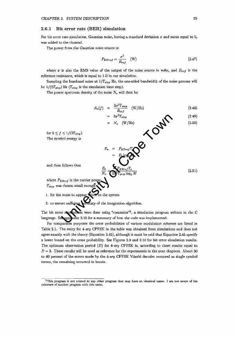
2.6.1 Bit error rate (BER) simulation
For bit error rate simulation, Gaussian noise, having a standard deviation CT and mean equal to 0,
was added to the channel.
The power from the Gaussian noise source is:
(W) (2.47)
where CT is also the RMS value of the output of the noise source in volts, and Hr.1 is the
reference resistance, which is equal to 1 n in our simulation.
Sampling the baseband noise at l/Tstep Hz, the one-sided bandwidth of the noise process will
be 1/(2T.tep) Hz (Tstep is the simulation time step).
The power spectrum density of the noise No will then be
for 0 :s; f :s; 1/(2Tstep).
The symbol energy is
and then follows that
where PESrel is the carrier power.
Tstep was chosen small enough
2CT2Tstep
Hrel 2CT2T.tep
(W/Hz)
= No (W/Hz)
Es = PESrelTs
Eb 1og2M
Eo PESTeIT.
No 2CT2T.tep log2 M
1. for the noise to appear white to the system
2. to ensure suffident accuracy of the integration algorithm.
(2.48)
(2.49)
(2.50)
(2.51)
The bit error simulations were done using "commsim,,3, a simulation program written in the C
language. See appendix 2.10 for a summary of how the code was implemented.
For comparison purposes the error probabilities of various modulation schemes are listed in
Table 2.1. The entry for 4- ary CPFSK in the table was obtained from simulations and does not
agree exactly with the theory (Equation 2.45), although it must be said that Equation 2.45 specify
a lower bound on the error probability. See Figures 2.9 and 2.10 for bit error simulation results.
The optimum observation period (D) for 4-ary CPFSK is, according to these results equal to
D = 3. These results will be used as reference for the experiments in the next chapters. About 30
to 40 percent of the errors made by the 4-ary CPFSK Viterbi decoder occurred as single symbol errors, the remaining occurred in bursts.
3This program is not related to any other program that may have an identical name. I am not aware of the existence of another program with this name.
Univers
ity of
Cap
e Tow
n

CHAPTER 2. SYSTEM DESCRlPTION
Peb
Ie+OO
.... FSK: theory I e..o I FSK: Tstep = Ts/20
MSK:theory
MSK: Tstep = Ts/40 le..o2 MSK: Tstep = Tsl20
le-03
le..o4
le..oS
Figure 2.9: BER results for MSK and FSK
Modulation scheme
BPSK
DPSK
QPSK and OQPSK
MPSK (M ~ 4)
Coherent Binary FSK
Noncoherent Binary FSK
MSK
GMSK
M-ary QAM
MFSK
4-ary CPFSK
Table 2.1: Pe equations for various modulation schemes
26
Univers
ity of
Cap
e Tow
n

CHAPTER 2. SYSTEM DESCRIPTION 27
1e+oO
-le-Ol
- = c--- ~ .... MSK:theory -"'~" - r-'. 4-aryCPFSK ~
- e D=I r=
le-02
".
'~~ r-
........ D=2 r-
~ , . i:s D 3 § -e- D-4 r-
" , \.
le-03
Peb
" • " '.
'.
10-04 ~
.. \
le-05 ~ '.
le-06 ~ "
1e-07 o 3 6 9 12 15
Figure 2.10: BER results for 4-ary CPFSK, Tstep == T s/40 Univers
ity of
Cap
e Tow
n

Chapter 3
Sequential Decoding Algorithms
3.1 Sequential Decoding
In this section we will describe sequential decoding and the Fano algorithm through a discussion
of its application to 4-ary CPFSK. Wozencraft [34] gives a very good description of sequential de
coding, including the Fano algorithm, but his discussion is based on an application to the discrete
binary symmetric channel.
Given a 4-ary CPFSK demodulator that provides us with a full set of metrics, let us consider
the outputs when the input is not corrupted by noise. The decoder starts at the root of the trellis,
read in all metrics associated with the branches diverging from this node and follows the branch
with the largest correlation (metric) to the next level node. Having thus been directed to a particu
lar next depth node of the trellis, the decoder again read in all metrics associated with the branches
diverging from this next level node and continue in this fashion. This works fine when no noise is
present. However, when noise corrupts our demodulator in such a way that one of the branches
diverging from the node under discussion receives a metric that is larger than the branch which is
suppose to give the largest metric, our decoder will initially proceeds along the incorrect path. I
say initially since it is possible that our path will cross the correct node farther down the trellis,
and it is possible that we may continue on the correct path from this point. This will obviously
result in an error in the decoding process. Once on the wrong path, the decoder is unlikely to
find any path stemming from the initial incorrect node which agrees well with the received sequence.
The idea of sequential decoding is to program the decoder to act much as a person who makes
a ''best'' choice at a cross-road on the basis of information laid before him about the short term
smoothness of the possible paths. If his best choice was an incorrect one, his path will soon be
come increasingly bumpy. He will intelligently choose a ''bumpyness'' threshold or discard criterion.
Violation of this threshold signals an incorrect decision somewhere back. He then goes back and
tries the other best choice. Even if he crosses the correct path on one of his future crossroads and
makes a correct decision, the effect of his previous incorrect choice is suppose to cleave to him, and
the effect of any further incorrect choices will add to this memory. The principle to be exploited is
that only at those rare times where we do make an incorrect decision do we need to go back and
investigate other best options.
Let us assume that the decoder has penetrated 1 intervals into the trellis, l ;::: O. Let d(l) denotes
the accumulated path metric observed by the decoder, between the tentative path it is follOWing
28
Univers
ity of
Cap
e Tow
n

CHAPTER 3. SEQUENTIAL DECODING ALGORITHMS 29
and the corresponding l-interval segment of the received sequence. As the decoder penetrates
deeper into the trellis, it maintains a running count of del). After each successive penetration
the decoder compares del) against a discard criterion function, .:l(t). If d(l) ever exceeds Ll(l),
the tentative path is discarded as too improbable. The decoder then backs up to the next best
unexplored branch for which del) :5 .:l(l) and starts moving forward as far as the discard criterion
function .:l(l) permits. If the tentative path is the correct path, then del) = 0 and Ll(l) will be
a constant. Due to noise del) will oscillate around this zero value. When the tentative path
departs from the starting node along the incorrect branch, we anticipate that del) will oscillates
about a line with an average slope (p - Vave ), where p is the branch metric value .:lAn(X, y) of its
corresponding received signal Sn(x, y) when no noise is present, while Vave will be the average of
the single largest metric available at each of the possible "incorrect" states. Thus, we cannot talk
about del) being a straight line as discussed by Wozencraft for the binary discrete case where the
Hamming distance between any two branches are a constant number of bits.
In our case, the distance is not equal, but is a function of the specific received symbol and
the present '~ncorrect" state from which we look forward. The instantaneous value of v will be
an element of a set of best metrics as seen from the possible "incorrect" states. The best possible
metrics1 (normalized) for 4-ary CPFSK as seen from an incorrect state, are listed in Table 3.1 as
obtained from Table 3.2. The maximum and minimum values of v are 0.32 and 0, respectively,
and the average value of the best possible metrics is Vave 0.125. A typical plot of del) can be
seen in Figure 3.1 showing an incorrect decision at interval 1.
d(l)
(p - vmin)l
= (0.5 0.0)1 = 0.501
(p - vma.,)l
= (0.50 0.32)1 = 0.18l
~(l2 ~t~~~t ___ _ o 1 2 3 4 5 6 7
Figure 3.1: Typical plot of del) showing incorrect decision at interval 1
Sy,o(t) 0.0,0.32 0.0,0.11 0.0,0.32 Sy,l(t) 0.0,0.32 - 0.0,0.32 0.0,0.11 Sy,z(t) 0.0,0.11 0.0,0.32 - 0.0,0.32 Sy,s(t) 0.0,0.32 0.0,0.11 0.0,0.32 -
Table 3.1: Set of Best Metrics as seen from "incorrect" state
values in the table are not highly accurate but rounded off in order to reduce the size of the metric alphabet and to simplify the examples that follow.
Univers
ity of
Cap
e Tow
n

CHAPTER 3. SEQUENTIAL DECODING ALGORITHMS 30
-0.32 -0.32 0.00 -0.11
Table 3.2: Normalized metrics for 4-ary CPFSK, Es = 0.5 J and Ts = 1 second.
Let us assume that the decoder need to penetrate at least K intervals, starting from node n, to
recognize an incorrect choice at node n - 1. Then our decoder may decode Un once it has analyzed
up to interval n + K without exceeding the discard criterion (threshold). The first basic concept
of sequential decoding is that the saving in the number of computations decrease exponentially as
K becomes smaller. With the threshold defined as 6., the worst case K for 4-ary CPFSK will be:
Kma:n ceil ( 6. ) p-Vmax
(3.1)
where P 0.50, Vma", = 0.32 and ceil(x) is the least integer greater than or equal to x. It is clear that the average number of computations is reduced by making 6. small, but if 6. is
too small, channel noise may cause many branches in the trellis to exceed 6., triggering a look-back
subroutine which slows down progress.
This lead to the definition of the second basic concept of sequential decoding: On these less
frequent occasions (given a reasonable SIN) when all branches are discarded, a less stringent cri
terion, such as a /unction 6.2 is invoked, or 6.s in more severe cases.
An algorithm that permits efficient and flexible implementation of these basic concepts was
devised by Fano [9].
3.2 The Fano algorithm
Fano adopted a "tilted" distance function, which I adapted for our application to the following
form:
tel) del) (p - '11)1 (3.2)
The corresponding discard criteria, called thresholds, are horizontal lines with spacing 6.. When
following the correct path, we have that tel) = -(p - '11)1.
As we update tel) along the way, a received "distance" tree is formed. A node of the received
distance tree is said to satisfy all thresholds that lie on or above it and to violate all thresholds
that lie beneath it. The tightest threshold satisfied by a node is the one that lies just on or above
it. Of the nodes diverging from any given node, the one with the largest metric is called the best
and the ones with smaller metrics are called worst.
The Fano algorithm maintains a running threshold, denoted by 5 and equal to k6., where k
is a (variable) integer. We say the running threshold is tightened when k is assigned so that 5 is
the tightest threshold satisfied by the search node, that is, by the node then being considered. An
essential feature of the algorithm is that we are not allowed to move either forward or backward
Univers
ity of
Cap
e Tow
n

CHAPTER 3. SEQUENTIAL DECODING ALGORITHMS 31
unless this can be accomplished without violating the running threshold; the running threshold is
raised only when necessary to accommodate such a move. The procedure is best explained by the
flow diagram in Figure 3.2 and the following examples. In the examples that follow, metric values
typical for Eb/No = 9.0 dB are used.
Yes
Start at Look forward Look back origin of to best, or if Are we from present RT
No violated best 1st
i-r'l"'" entering via at the r----- position to
branch; [Alnext origin? previous RTat 0 best node node
•
RT RT satisfied satisfied
~ Move back Increase
RTby A
Are we Did move
No at this Yes originate node on a -- for the worst
1st time? node?
No
Yes RT; Running Threshold (8)
~
Tighten RT if
possible
Figure 3.2: The basic Fano Algorithm
Example 1: (p - v) 0.30 R; (p - Vave ); A 0.30
Given the received sequence as in Figure 3.3, let us assume that we've been following the correct
path but make an erroneous decision at the 3rd interval (indicated by a *). Table 3.3 and Figure 3.4
show the tree searching progression.
The algorithm failed to detect the incorrect path early enough, and re-merging with the correct
path occur, resulting in an error event as shown by the dotted line on Figure 3.3. The following
should be considered when trying to explain the failure of the algorithm for this example:
1. The smaller the value of (p - v), the higher the likelihood that the look-back subroutine
will be triggered unnecessary, especially when t(l) are just below the running threshold. H
Univers
ity of
Cap
e Tow
n

CHAPTER 3. SEQUENTIAL DECODING ALGORITHMS 32
state
S3 '
S2 '
SI '
Error event ~ ....
so (Exam~le 1 and ~,a) , ',,'
Figure 3.3: Received sequence for Example 1 and 2.a
I At I 0 I action I ~An(X,y) I d(l) I tel) I action 0 0.00 look at 1 0.40 0.10 -0.20 move to 1 1 0.00 look at 2 0.43 0.17 -0.43 move to 2, set 0 = -0.30 2 -0.30 look at 3 0.49 0.18 -0.72 move to 3, set 0 = -0.60
• 3* -0.60 look at 4 0.40 0.28 -0.92 I move to 4, set 0 = -0.90 4* -0.90 look at 5 0.38 0.40 -1.10 move to 5
I 5* -0.90 look at 6 0.28 0.62 -1.18 move to 6 ~lookat7 0.21 0.91 -1.19 move to 7
7 look at 8 0.51 0.90 -1.50 move to 8, set 5 = -1.5 8 -1.50 look at 9 0.49 0.91 -1.79 move to 9 9 -1.50 look at 10 0.48 0.93 -2.07 move to 10, set 5 = -1.80 I
Table 3.3: Tree search for Example 1 ((P - v) 0.3, and ~ = 0.3)
required, the Fano algorithm will increase the running threshold in order for the algorithm
to continue, however, unnecessary computations will result,
2. If the value of (p-v) is too large, the look-back subroutine may not be triggered soon enough,
or more likely, not at all when on an incorrect path,
3. The smaller ~, not only will tel) reach the next lower threshold sooner and thereby increasing
the probability of the event in 1, but the look-back subroutine will in general be triggered
(perhaps unnecessary) with higher probability depending on the noise level, resulting in
unnecessary computations,
4. When ~ is too large, the look-back subroutine may be triggered too late, resulting in too
many unnecessary move-back computations. This will especially be the case when tel) is just
above the next lower threshold. In fact, if (P-v) is chosen too large, the look-back subroutine
may never be triggered when necessary.
Choosing the above parameters incorrectly may result in catastrophic failure in that the algorithm
progresses very slowly or not at all, or it may result in too many error events caused by re-merging
of the correct and tentative path we are following. In the following example we reduce the values
of (p - v) and ~ on the basis of argument 1 and 2 above.
Example 2.a: (p - v) = 0.20; ~ = 0.20
See Table 3.4 and Figure 3.5.
Although the look-back routine was triggered, the algorithm still failed to detect the incorrect decision before re-merge.
Univers
ity of
Cap
e Tow
n
CHAPTER 3. SEQUENTIAL DECODING ALGORITHMS 33
0.0
-n.3
-0.6
-0.9
-1.2
-1.5
-1.8
-2.1
1m
0.0
-0.2
-0.4
-0.6
-0.8
1(1)
~--------------------------------------------------~l
. , . . . . · , . . . . . ...... ';" ...... ;..... .. f'J' .... ';" ....... : ......... ! ......... :......... ......... .. ......... ..
.::::::.:t:.:::.:: j::::::::: f:': ::: ::j·~·:·:·:·:·:·:·:·n:.:.:.:.:.~:.~:.:.:.~~::::~:::::::: ::::::::: :::::::: ....... . , . , , . . . · . . , . . . · , , , . , .
~ ............... ~ .... ~ ................................................. -. . . . . . . . . . . . . . .. ......... _ ...... . · . . , . , . . , . , . . . . . : : : : : : : : 9 ............................................................................................................ , . , , , . . . · . . , . . . . , . , . . . . . , . , , , . . . ........................................ , ............... ·····r·········.··········,········· ................ . , . . . , . . . , . . , . . . . , . . , . . . , · . , . . . . .
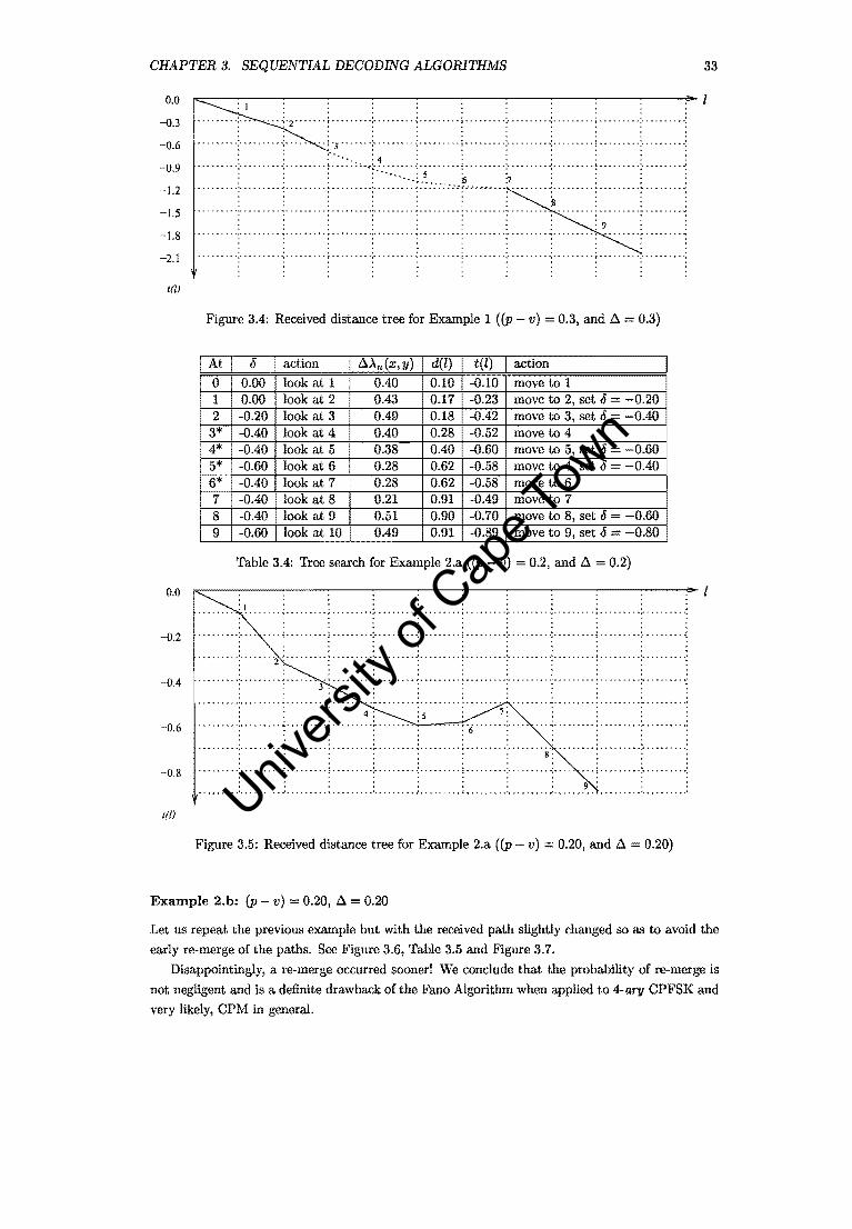
Figure 3.4: Received distance tree for Example 1 ((P - v) = 0.3, and .6. = 0.3)
action
move to 1 0.17 move to 2, set 0 = -0.20 0.18 -0.42 move to 3, set 0 -0.40 0.28 -0.52 move to 4 0040 -0.60 move to 5, set 0 -0.60 I
0.28 0.62 -0.58 move to 4, set 0 = -0040 I 0.28 0.62 -0.58 move to 6
look at 8 0.21 0.91 -0.49 move to 7 8 look at 9 0.51 0.90 -0.70 9 look at 10 0.49 0.91 -0.89
Table 3.4: Tree search for Example 2.a ((P - v) = 0.2, and .6. = 0.2)
~------------~------------------~----------------~l
........ : L ...... ; ......... ; ......... : .......... : ......... ; ......... : .......... : ......... ; ......... : ....... .. , , . . . . . . . . · , . . . . . . . , · , . . . . . . . .
•••••• ~ • .;.~ ••••••• : •• ~ ••• ~ •• ;~ ••• ~ ••• ~: •••••••••• ;. •••••••• : •••••••• .; •••••••••• : •••• " ••• ; 0 •••••••• :~ ••••••••
, , . . . . . . . . · , . . . . . . , , · , . . . . . . . , ......•. ';" •...... 2 ':' .....•. ': •... 0 .... ;, ... _ .... ';, ........ :' ...... 0':' ........ '; ......... : ........ ':' ...... ,-· ,.,...,' · , . , . , . . , . • •••••••• ' ••••••••• " • • • •• • ~ ••••••••• ' .................... ~ .................... ' •• - •••••••••••••••• ' ••• « ••• ~ •
: : 3 . : : : : : : : .. .....,. , . , , , . . . . .
• .................. -. • • • • • • • • • • • • • • • ••• • • • • • • • • ... • • • • • • • • • • • • • • • • • • ••••••• - ••••••••••••••• « ........... ~ • , .. .. . . : : : 4 : : 5 : .: : ......... ; ......... ; ......... : ......... :......... ·····:·6·······:·······:·········:········ ';" ~ ... ,. · . .. ..... · . . , " '.. · .... , .. ; ......... ; ......... : ......... ; ......... : ......... : ......... : .... , ... 8': ........ : ... , ..... ; ....... . · , , , . , , , . . , . . . . . , , . . · ..... ". ," . " .. , ... ',' .. " . , . , . : . , , , . , . , '.' .... , , " , '.' " . , ..... : . " .... , . '," ........ ',' .. ' . . . ~ ..... , .. ',' ....... . , . , . . , . , . ,
......... :...... .; ........ ; ......... : .......... : ......... ; ......... : ....... : ..... ~.: ....... : ...... ..
Figure 3.5: Received distance tree for Example 2.a ((P - v) :;:; 0.20, and .6. 0.20)
Example 2.b: (p - v) = 0.20, .6. = 0.20
Let us repeat the previous example but with the received path slightly changed so as to avoid the
early re-merge of the paths. See Figure 3.6, Table 3.5 and Figure 3.7.
Disappointingly, a re-merge occurred sooner! We conclude that the probability of re-merge is
not negligent and is a definite drawback of the Fano Algorithm when applied to 4-ary CPFSK and
very likely, CPM in general.
Univers
ity of
Cap
e Tow
n
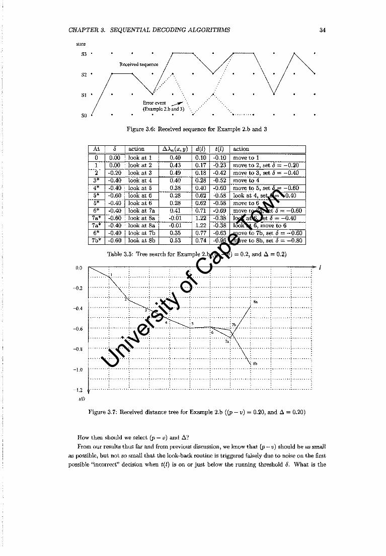
CHAPTER 3. SEQUENTIAL DECODING ALGORITHMS
state
83
Received sequence
82 •
81 • . .•.
80
0.0
-0.2
-0.4
-0.6
-0.8
-1.0
-1.2
tal
Error event --"",,". . . (Example 2.h and 3) ........ . '
Figure 3.6: Received sequence for Example 2.b and 3
~t I 11 I action I aAn(X,y) I del) [ tel) I action
0 0.00 look at 1 0040 0.10 -0.10 move to 1 1 0.00 look at 2 0.43 0.17 -0.23 move to 2, set 11 = -0.20 2 -0.20 look at 3 0049 0.18 -0042 move to 3, set 11 = -0040
3* -0040 look at 4 0040 0.28 -0.52 move to 4 4* -0040 look at 5 0.38 0.40 -0.60 move to 5, set 11 - -0.60 5* -0.60 look at 6 0.28 0.62 - look at 4, set 11 = -0040 5* -0.40 look at 6 0.28 0.62 - move to 6 6* ~lookat7a 0041 0.71 -0.69 move to 7a, set 11 = -0.60 7a* - . look at 8a 1 1.22 -0.38 look at 6, set 11 0040 7a* -0040 look at 8a -0.01 1.22 -0.38 look at 6, move to 6 6* -0.40 look at 7b 0.35 0.77 -0.63 move to 7b, set 11 = -0.60
7b* -0.60 look at 8b 0.53 0.74 -0.96 move to 8b, set 11 = -0.80
Table 3.5: 'free search for Example 2.b ((P - v) 0.2, and a = 0.2)
......... :1. . . . , . . . . . • _ • .,W ••••••• , r •• , ••• 0 " '.~ , •• " •••• 0,' •••••••• r •••• " • " • ".' •• " • - ••• '.' •••••••• 1 ••• , ••• ~ • " " , ••• __ •
......... : ..... , ... : ........ : ......... ; .......... : ......... : ......... ;. ........ ·:·········f·········:····· .. , . . . . . . . . . · . . . . . . , . . , . . . . . . . . .
• 0000.00 or 0 ..... 2: .. 0 ... o. 0 ~ 0 ... 0 .... ~ ......... ':' 0 ... 0 0 0 0: 0 .. 0 0 ... 0: ........ ":0 ~~ ... 0 .. : 0 ..... 0 0 .~ ....... .
· . . . . . , . . . · ........ '. .. .. . ., ..... ~ . , . . . . . . . . .... ... . . ... . . . . . . . . . . . . . . .. .'......... . ........................... . : : 3 . : : : : : : : .. .,..... · . . , . . . . . .
.............................................. ~ ••••••• 4 ................ _ ••••••••••••• ~ ........ ~ ••• ~ · .. ..... . : : : 4 : : s: ::: ................ ........................... ..... -.. · . - . , . . . · . . . · . . . " '.. ....... : ....... 0: .. 0 ...... ; ....... ":'" ...... ;0 ........ : ...... 'i~:" ....... : ......... : ........ : ........ · , . . .. '.. · ...... ~ .: .. ~ ...... ~ ... --.. -. : . -... -... :~ ... -... -.:. --...... ; . . .. . ... :. . . .. . ... : ... -..... : ......... : ........ -· . . . . . . . , , · . . . . . . . , . · . . . . . . . . . · ....... .; .......... :. -. ~ . -. -. ;. ........ -: .... ~ . -. ~ .:- . -. -. -. -: .. -. -. -. -;- .. -.. ,~ -;- -....... : ..... , -.. :. -... --.. : : : : : : : . 8b : : · . . . .. .. · .... -. , .. ,. . ..... " ... ~ . -. . . . .. .. -. , .' ............... -... -. -. -. -. -.. ' ........... ', ............. -........ --. ---· . . . . . . . . . · . . . . . . . . . · . . . . . . . . . · . . . . . . . . .
~ ••••••• '" ~..... .. ••••• & • < • ~ ••••••• , '" ., • ~ ~ .......... - ••••• ~. • •• , ................ ," - ••• - •• • ......... - • - • -· . . . . . . . . . · . . . . . . . . . , . . . . . . . . . · . . . . . . . . . •••••••• " •••••••• ~ ••• _. _. _ ................................. -~ ••• ~ •• " ••• - •••• ~ ••••••••• - ••••• ~. &~ ••••••••
Figure 3.7: Received distance tree for Example 2.b ((P v) = 0.20, and ~ = 0.20)
How then should we select (p - v) and ~?
34
From our results thus far and from previous discussion, we know that (p - v) should be as small
as possible, but not so small that the look-back routine is triggered falsely due to noise on the first
possible ''incorrect'' decision when tel) is on or just below the running threshold 11. What is the
Univers
ity of
Cap
e Tow
n

Report on corrections to Masters dissertation
Werner F Kleyn
31 May 2002
The following corrections have been done:
1. Lower case 'c' replaced by upper case 'C ' where reference is made to specific chapters.
Applicable page: 13.
2. Lower case 'e' replaced by upper case 'E' where reference is made to specific equations.
Applicable pages: 14, 17, 18, 19, 23, 24, 25, 26, 35, 52, 54.
3. Lower case 'f' replaced by upper case 'F' where reference is made to specific figures.
Applicable pages: 14, 18, 19, 21, 22, 26, 29, 31, 32, 33, 35, 36, 38, 47, 48, 49, 52,
58, 61.
4. Lower case 't' replaced by upper case 'T' where reference is made to specific tables.
Applicable pages: 26, 29, 32, 33, 36, 51, 54, 58, 60, 61.
The following have been added:
1. A short conclusion chapter (Chapter 5) including summary and a future work section. Table of
contents were updated.
Signed:
(student) (supervisor)
(date) (date)
Univers
ity of
Cap
e Tow
n
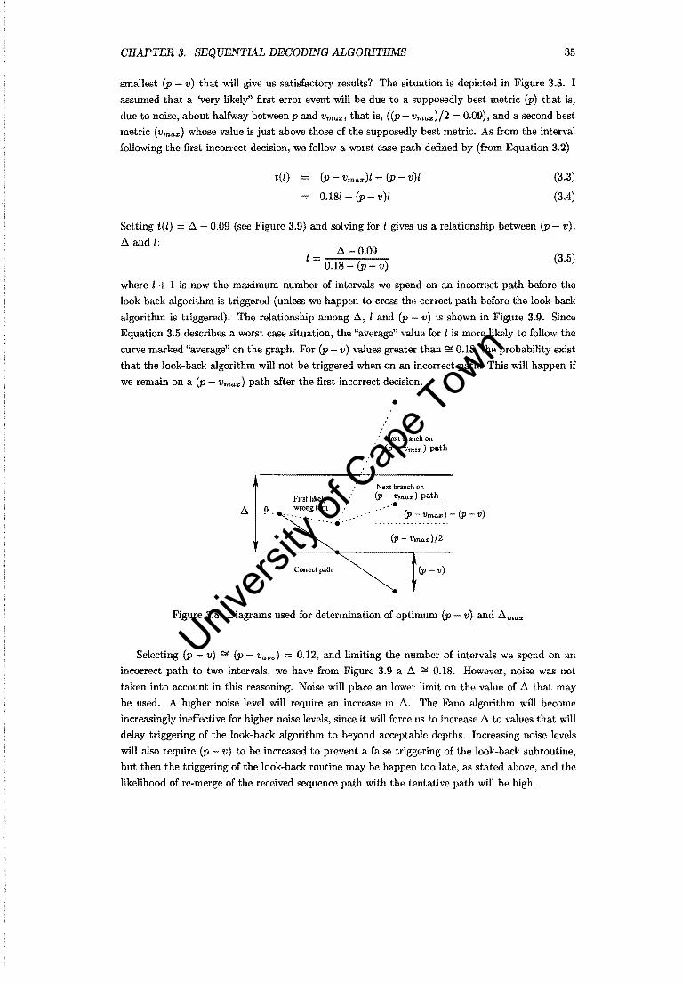
CHAPTER 3. SEQUENTIAL DECODING ALGORITHMS 35
smallest (p - v) that will give us satisfactory results? The situation is depicted in Figure 3.8. I
assumed that a "very likely" first error event will be due to a supposedly best metric (P) that is,
due to noise, about halfway between p and Vrn""" that is, «P- vrn"",)/2 = 0.09), and a second best metric (vrn"",) whose value is just above those of the supposedly best metric. As from the interval
following the first incorrect decision, we follow a worst case path defined by (from Equation 3.2)
t(l) = (p - vm"",)l - (p - v)l
0.181- (p - v)l
(3.3)
(3.4)
Setting t(l) = .6. - 0.09 (see Figure 3.9) and solving for 1 gives us a relationship between (p - v),
.6. and 1: 1= .6. - 0.09
0.18 (p - v) (3.5)
where 1 + 1 is now the maximum number of intervals we spend on an incorrect path before the
look-back algorithm is triggered (unless we happen to cross the correct path before the look-back
algorithm is triggered). The relationship among .6., I and (p v) is shown in Figure 3.9. Since
Equation 3.5 describes a worst case situation, the "average" value for I is more likely to follow the
curve marked "average" on the graph. For (p - v) values greater than ~ 0.18, the probability exist
that the look-back algorithm will not be triggered when on an incorrect path. This will happen if
we remain on a (p vm ,,"') path after the first incorrect decision.
.6. . P .. First likely wrong tum .... . ..•...
: Next branch on . (p - 11m;n) path
Next branch on (p - 11m"",) path ...
(p vm"",) (p - v)
{p - vma",)/2
(p -v)
Figure 3.8: Diagrams used for determination of optimum (p v) and .6.m "",
Selecting (p - v) ~ (p v"ve) = 0.12, and limiting the number of intervals we spend on an
incorrect path to two intervals, we have from Figure 3.9 a .6. ~ 0.18. However, noise was not
taken into account in this reasoning. Noise will place an lower limit on the value of .6. that may
be used. A higher noise level will require an increase in.6.. The Fano algorithm will become
increasingly ineffective for higher noise levels, since it will force us to increase .6. to values that will
delay triggering of the look-back algorithm to beyond acceptable depths. Increasing noise levels
will also require (p - v) to be increased to prevent a false triggering of the look-back subroutine,
but then the triggering of the look-back routine may be happen too late, as stated above, and the
likelihood of re-merge of the received sequence path with the tentative path will be high.
Univers
ity of
Cap
e Tow
n

CHAPTER 3. SEQUENTIAL DECODING ALGORITHMS 36
10
5
Ll= 0.50 Ll = 0.24
Ifaveragelf
Ll = 0.24
./ -- Ll =0.15
0 0 0.D3 0.06 0.09 0.12 0.15 0.18 0.21
p-v
Figure 3.9: Relationship among ~, (p - v) and l.
Example 3: (p v) 0.12; ~ = 0.18
In this example, we will let (p - v) = 0.12 and ~ = 0.18. See Table 3.6 and Figure 3.10.
I At I 15 I action I ~An(X,y) I d(l) I t(l) I action 0 0.00 look at 1 0.40 0.10 -0.02 move to 1 ;
1 0.00 look at 2 0.43 0.17 -0.07 move to 2 2 0.00 look at 3 0.49 0.18 -0.18 move to 3, set 0 = -0.18 '
~~.18 look at 4a 0.40 0.28 -0.20 move to 4a -0.18 look at 5a 0.38 0.40 -0.20 move to 5a -0.18 look at 6a 0.28 0.62 -0.10 look at 4a, move to 4a
4a* -0.18 look at 5b 0.30 0.48 -0.12 look at 3, move to 3 3 -0.18 look at 4b 0.38 0.30 -0.18 move to 4b
4b -0.18 look at 5c 0.54 0.26 -0.34 move to 5c 5c -0.18 look at 6b 0.48 0.28 -0.44 move to 6b 6b -0.36 look at 7 0.58 0.20 -0.64 move to 7
Table 3.6: Tree search for Example 3 «(p - v) 0.12, and ~ = 0.18)
It seems that the likelihood of the two paths re-merging is not negligent. However, this time the
incorrect decision was detected despite the re-merge. However, noise almost cause the algorithm
to trace back further than was necessary on its second visit to node 3.
3.2.1 Simulations
Simulations applying the Fano algorithm to decoding 4-ary CPFSK were performed for the fol
lowing combinations of (p - v), ~ and Eb/No :
Eo/No = 16.00,13.10,11.94,10.00 and 8.42 dB
Univers
ity of
Cap
e Tow
n

CHAPTER 3. SEQUENTIAL DECODING ALGORITHMS 37
0.0 . . . . ,
...... ~ •• •• t •••••••• '.' •••••••• ',' •••••••••
: 6.
4b: ......... ' ........ " ....... "'1-=~:::::':'::':':':> : : 3: :: 4a: .
-0.18
· ~ .. . ... -......... ". . . . .. .. ~ ........ '. .. . ......................... '.. ... .. · . . . . . . · . . . . . . · . . . . . . · . . . . . . • ••••••• '" • • • • • •• .. ••••••••• ~ ••••••••• 0 ••••• _. • .............................. . · . . . . . . · . . . . . .
: : : : . 50: : -0.36 ............................. _" • __ •• _. __ 0 •• '0."", .0 ••••••••••• _ ••• p •• o. _ •• _ · . . . . . . · . . . . . . · ., · . . .
• • • • • •• ",'. ••• • .... ~ ••••••• t - ••• - • - • -,' - ••• - • - • • • •• • f ••••••••
: : : . 6b. . . . . . . . · . . . . . , ............................. : .............................. ; ..... ',--"--'" · . . . . . . · . . . . . . · . . . . . . -0.54 · ........ :- ........ -;. ........ : ......... : .......... :- ........ : . . .. . .. -:. ~ ...... . · , . . . . . . . . . . . .. .. ~ . . .. .: ........ .
· , . . . . . , . . . . . . •••••••••••••••••••• ' ••••••••• \ .............................. 1 ••••••••• • ••••••••• · . . . . . . , . . . . . .
: : : : : : . 7 ................................................................................ . , . . . , . 1(1)
Figure 3.10: Received distance tree for Example 3 «P - v) == 0.12 and Ll = 0.18)
(p - v) 0.06, 0.09, 0.12, 0.15 and 0.18
Ll = 0.06, 0.09, ... 0.27 and 0.30.
The following data was recorded:
1. Number of symbol errors
2. Number of burst errors
3. Total number of look-backs
4. Total number of move-back steps
5. Distribution of instantaneous move-backs steps (the number of times that we moved back a
specific number of steps)
6. Distribution of maximum depth reached in moving back at each new set of metrics investi
gated
The Fano decoder was simulated on a pseudo-random sequence of 200000 input bits, except for the
tests where Eb/No = 16.00 dB and Eb/No = 13.10 dE. At these signal-to-noiseratios 10 million and
1 million input bits were used, respectively. The degree of the pseudo-random generator polynomial
used was 18. One might question whether this procedure is appropriate, but the results obtained
nevertheless show valuable information as to the suitability of the Fano algorithm for decoding
schemes with variable distance between signal sets. A more appropriate method would have been
to run the simulations until i.e. 50 symbol errors were generated. In the graphs that follows, all
the results were normalized to 100000 input symbols (200000 bits). For these tests a simulation
step size of Ts /20 seconds were used. The Fano algorithm's memory were limited to 12, that is, all
metrics were saved to a depth of 12 and then discarded. This means that whenever the move-back algorithm tried to move back more than 12 intervals, the algorithm reacted as if it has reached
the origin (see the flow chart in Figure 3.2), These attempts to exceed a depth of 12 backward
moves are recorded in the bar charts that follow, as a '> 12' tick. An observation period (number
of symbol intervals observed before making decision about the 1st symbol transmitted) equal to
12 was used.
Univers
ity of
Cap
e Tow
n
CHAPTER 3. SEQUENTIAL DECODING ALGORITHMS 38
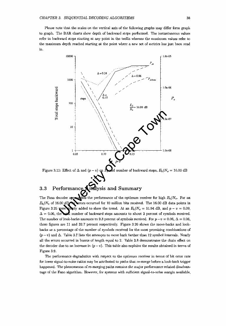
Please note that the scales on the vertical axis of the following graphs may differ form graph
to graph. The BAR charts show depth of backward steps performed. The instantaneous values
refer to backward steps starting at any point in the trellis whereas the maximum values refer to
the maximum depth reached starting at the point where a new set of metrics has just been read
in.
"'Cl ta ] (.) o;l
.c '" ~ '" "a '"-' 0
E-<
10000
\ b. =0.24
1000
/
/
100
10
/ /
/ /
/ /'
/
Eb -= 16.00 dB No
l.Oe-05
l.Oe-06
1.0e-07
I +-~~~~~~..-~--i-..l.,--r'-~.,........,,....~~~~~,.-l- l.Oe-OS 0.05 0.10 0.15
p-v
Figure 3.11: Effect of ~ and (p - v) on p. and number of backward steps, Eb/No 16.00 dB
3.3 Performance Analysis and Summary
The Fano decoder approaches the performance of the optimum receiver for high Eb/No. For an
Eb/No of 16.00 dB, no errors occurred for 10 million bits received. The 16.00 dB data points in
Figure 3.25 were simply added to show the trend. At an Eb/No 11.94 dB, and p - v = 0.09,
~ = 0.06, the total number of backward steps amounts to about 2 percent of symbols received.
The number of look-backs amounts to 9.3 percent of symbols received. For p - v 0.06, ~ = 0.06,
these figures are 11 and 32.7 percent respectively. Figure 3.26 shows the move-backs and look
backs as a percentage of the number of symbols received for the most promising combinations of
(p v) and ~. Table 3.7 lists the attempts to move back farther than 12 symbol intervals. Nearly
all the errors occurred in bursts of length equal to 2. Table 3.8 demonstrates the chain effect on
the decoder due to an increase in (p - v). This table also explains the results obtained in terms of
Figure 3.9.
The performance degradation with respect to the optimum receiver in terms of bit error rate
for lower signal-to-noise ratios may be attributed to paths that re-merge before a look-back trigger
happened. The phenomenon of re-merging paths remains the major performance related disadvan
tage of the Fano algorithm. However, for systems with sufficient signal-to-noise margin available,
Univers
ity of
Cap
e Tow
n
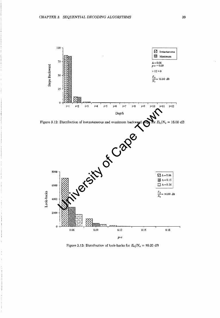
CHAPTER 3. SEQUENTIAL DECODING ALGORITHMS 39
100 0 Instantaneous
~ Maximum
75 A=O.06 1: p-v =0.09
~ > 12=0 ~ u
'" 50 Eb il:)
'" -= 16.00 dB Cl. No ~ <Zl
25
i=! i=2 i=3 i=4 i=5 i=6 i=7 i=8 i=9 i=10 i=l1 i=12
Depth
Figure 3.12: Distribution of instantaneous and maximum backward steps for Eb/No = 16.00 dB
8000
6000
J:l g ~ 4000 0 0
...l
2000
0 0.06 0.09 0.12
p-v
0.15
o A=0.06
~ A=0.15
El A=0.24
0.18
Figure 3.13: Distribution of look-backs for Eb/No 16.00 dB
Univers
ity of
Cap
e Tow
n

CHAPTER 3. SEQUENTIAL DECODING ALGORITHMS 40
10000 I.0e"()2
\
1000 tOe-03
"0 ~
~ u Pe ~ .,
Peb '" 100 I.Oe-04
B-". -
'" 3 0 r-
IO /' /' 1.0e"()5 /' /'
/' /' "-/' /'
/' /'
1 1.0e-06 0.05 0.10 0.15
p-V
300 ~ Instantaneous
~ Maximum
225 ~ 0.06 "1:1 p-v 0.09 !;j
> 12=0 ] u 0$ ISO
14.44 dB ill
'" Q. G.) .....
\Zl
75
i=l i=2 i=3 i=4 i=5 i=6 i=7 i=9 i=IO i=ll i=12
Depth
Figure 3.14: Distribution of instantaneous and maximum backward steps for Eb/No = 14.44 dB
Univers
ity of
Cap
e Tow
n
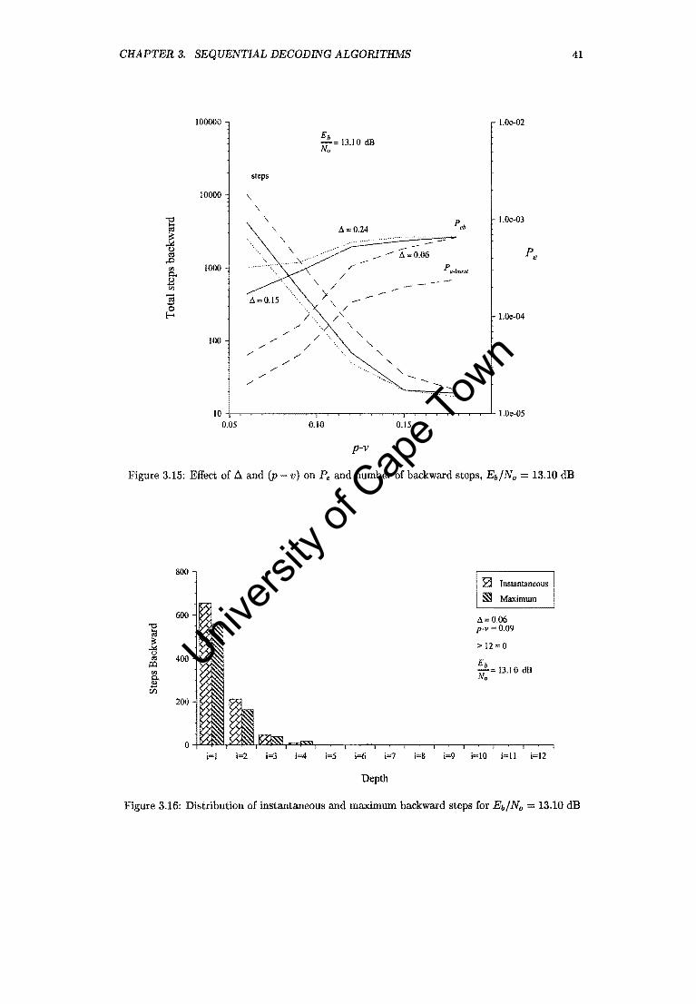
CHAPTER 3. SEQUENTIAL DECODING ALGORITHMS
100000
steps
10000 \ \
"E \
] \
~ ,J:J til 1000 Q.. CI.l -til ] 0
E-<
100 /' /'
/'
/' /'
./
10 0.05
\ \
./ /'
./ /'
Eb -= 13.10 dB No
A=0.24
__ -- i=0.06
\ "'-
"'-"'-
"'-"'-
0.10 0.15
p-v
41
1.0e-02
Peb l.Oe-03
Pe
P e--hurst
1.0e-04
1.0e-05
Figure 3.15: Effect of 6. and (p v) on Pe and number of backward steps, Eb/Na = 13.10 dB
800 ~ Instantaneous
~ Maximum
600 A=O.06
1 p-v = 0.09
~ > 12=0 <.:)
400 0;
ill 13.1 0 dB '" 0..
OJ
til 200
i=1 i=2 i=3 i=4 i=5 i=6 i=7 i=8 i=9 i=10 i=1I i=12
Depth
Figure 3.16: Distribution of instantaneous and maximum backward steps for Eb/Na = 13.10 dB
Univers
ity of
Cap
e Tow
n

CHAPTER 3. SEQUENTIAL DECODING ALGORITHMS
22500
~ 15000
.P
~ o ....l
7500
0.06 0.09 0.12
p-v
0.15
0t.-O.06! ~ I'. = 0.15j
· []t.=0.24
13.10 dB
0.18
Figure 3.17: Distribution of look-backs for Eb/No = 13.10 dB
100000 1.0e-0i Eb -= 11.94 dB No
steps
" 10000 " " " "0 " 1.0e-02 ;; " ] " ~ " Peb Pe ..0 " '" 1000 " c..
~ -a pc•burst ..... 0
r,-. 1'.= / )..-- 1.0e-03 0.15
/ --.. / --..
100 / 1'.=0.06/ ./ / ./
/ ./
/' / /
/ / /
/
10 1.0e-04 0.05 0.10 0.15
p-v
42
Figure 3.18: Effect of A and (p - v) on Pe and number of backward steps, Eb/No 11.94 dB
Univers
ity of
Cap
e Tow
n
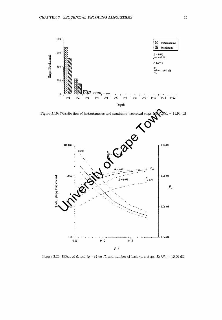
CHAPTER 3. SEQUENTIAL DECODING ALGORITHMS 43
1600 0 Instantaneous
~ Maximum
1200 A=0.06
] p-v =0.09
~ > 12=0 (,)
'" 800 ~ Eb til -= 11.94 dB
~ No
CfJ
400
i=1 i=2 i=3 i=4 i=5 i=6 i=7 i=8 i=9 i=lO i=11 i=12
Depth
Figure 3.19: Distribution of instantaneous and maximum backward steps for Ell/No 11.94 dB
100000 1.0e-Ol
steps Eb
"\ -=10.00 dB No
"\ "\
"\ Peb "\ A =0.24 "\
~ 10000 1.0e-02
~ 'y/ A ",0.06 Pe-burst
u "- Pe '" A= "-..0 (lJ 0.15 ./ /"-« p. ,/
"-Q.) ,/ - ,/ "-(lJ ./ "-";j /"
"-- / 0 ,/ "-t-< 1000
"-1.0e-03
"-
100 +-~~~~~~-r-~~~~~~,---,.~~~~~,........L.1.0e-04 0.05 0.10 0.15
p-v
Figure 3.20: Effect of 6 and (p - v) on Pe and number of backward steps, Ell/No = 10.00 dB
Univers
ity of
Cap
e Tow
n

CHAPTER 3. SEQUENTIAL DECODING ALGORITHMS 44
6000
0 Instantaneous
~ Maximum
'" 1::,=0.06 "0 4000 p-v = 0.09 a ~ > 12=4 ~ u 0:1
Eb o:l
'" -= 10.00 dB
0. No E 2000 rJ:l
i=1 i=2 i=3 i=4 i=5 i=6 i=7 i=8 i=9 i=IO i=11 i=12
Depth
Figure 3.21: Distribution of instantaneous and maximum backward steps for Eb/No = 10.00 dB
"0 liS ~ U 0:1
.J:J Vl 0. Q) -Vl
"@ -0 E-<
100000
10000
1000
I::, -" 0.15 "
/ ..,-
/ ./
/.
/ /
1.0e-01
~.;::"' ... - 1.0e-02 -....
-.... -....
-.... Pe -.... --steps'" '.
". -- -- --1.0e-03
Eb -= 8.42 dB No
100 +--~~~~~...,~~-~~~-.~~---~,......L.1.0e-04 0.05 0.10 0.15
p-v
Figure 3.22: Effect of.6. and (p - v) on Pe and number of backward steps, Eb/No = 8.42 dB
Univers
ity of
Cap
e Tow
n
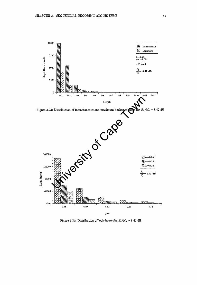
CHAPTER 3. SEQUENTIAL DECODING ALGORITHMS 45
10000 tl"l Insmntaneous
0 Maximum
7500 A=0.06 '" "0 p-v 0.09 a
~ >12 46 (,)
5000 '" Eb iJ:l
'" -= 8.42 dE
0.. No 2 en
2500
i=1 i=2 i=3 1=4 1=5 i=6 i=7 1=8 i=9 i=lO i=11 i=12
Depth
Figure 3.23: Distribution of instantaneous and maximum backward steps for E,,/No = 8.42 dB
161000 0A=0.06
tl"lA=O.15
121000 !ill A =0.24
en Eb ..I<: -= 8.42 dE g No ..0 81000 ..::!:: 0 0
....l
41000
0.06 0.09 0.12 0.15 0.18
p-v
Figure 3.24: Distribution of look-backs for E,,/No = 8.42 dB
Univers
ity of
Cap
e Tow
n
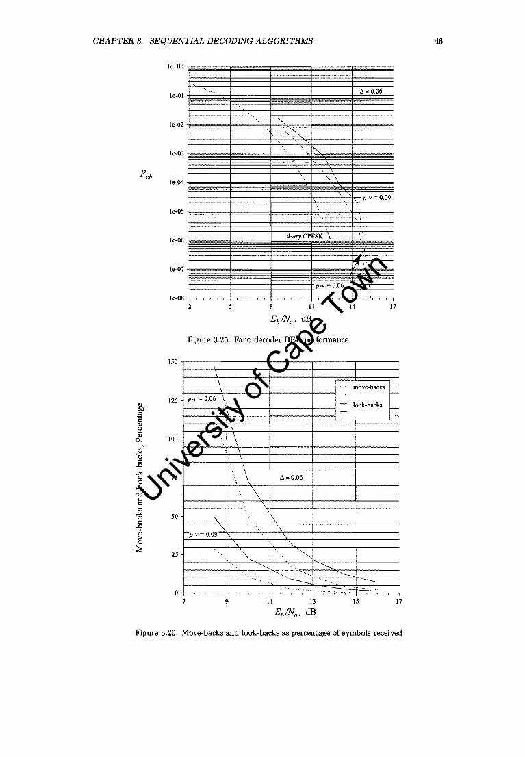
CHAPTER 3. SEQUENTIAL DECODING ALGORITHMS
Peb
leo02 ......
le-03
le-04 \\
p-v 0.09
Ie-OS
leo06 4-ary CPFSK \
Ico07 7"
p-II 0.06 I , .
leo08 2 5 8 11 14 17
EblNo' dB
Figure 3.25: Fano decoder BER performance
150~-------'-------'--------~------'1---------
\ \ \
125 P-II = 0.06 \
1\ \
100 \ , \
\
75
50
0.09 I'\.
\
\ \
\
....
25 ..... ~
I
move-backs --
look-backs --
a=O.06
\
\ "'" \
r-----~--~~-+-,,~ .... -=---'-~~=-----.«" .... ". ---
O+-~--~-t-~~---t~-
7 9 15 17
Figure 3.26: Move-backs and look-backs as percentage of symbols received
46
Univers
ity of
Cap
e Tow
n

CHAPTER 3. SEQUENTIAL DECODING ALGORITHMS 47
performance is acceptable. The problem of re-merging paths may be reduced by using schemes with
a longer minimum distance error event (schemes with larger constraint length for which applying
the Fano decoder would be more appropriate anyway, since exponentially increasing complexity
of the Viterbi decoder with increase in constraint length was in the first place the motivation for
using the Fano algorithm). Future research on the subject of Fano decoders should therefore focus
on a scheme with larger constraint length.
The Fano algorithm is substantially more complex to implement in software than the Viterbi
algorithm. This ratio of complexity (about 3 to 4) between the software implementations of the
Fano algorithm and the Viterbi algorithm can be expected to project to their respective hardware
(VLSI) implementations. On the other hand, whereas the memory required for implementation of
the Viterbi algorithm increases exponentially with constraint length of the scheme, it remains a
constant for the Fano decoder. Further investigation is required into the VLSI structure for the
Fano decoder.
I EMN" , dB I p - v I
0.06 I 0.09 16.00 0 0 14.44 2 0 13.10 26 0 11.94 63 0 lO.OO 280 4 8.42 747 46
Table 3.7: Number of attempts to move back deeper than 12 symbol intervals for .a. = 0.06
(p- v) t + look-backs + move-backs terrors • tl t prob (remerge)
t prob (move-back farther than 12)
Table 3.8: Effect of the increase of (p - v), .a. constant
Univers
ity of
Cap
e Tow
n

Chapter 4
Neural Network-based Receivers
4.1 Introduction
Contrary to conventional serial computers, neural net models explore many competing hypotheses
simultaneously by using parallel nets composed of many computational elements connected by links
having variable weights [15]. These computationalllnks are also called neurons or perceptrons.
The neural net stores experimental knowledge through a learning process as weights on the input
nodes to the neurons. Since finding the optimum path through a phase trellis can be related to
the problem of exploring many hypotheses simultaneously, we may postulate the artificial neural
net it to be a good trellis decoder. However, research [32, 18] done on the neural net's ability as
trellis decoder has produced very disappointing results. Most of these research focussed on using
very complex neural net structures. I will explore the subject by concentrating on very simple
structures.
The first part of this chapter provides an overview of neural nets in general. We will classify spe
cific neural nets according to the type of problem it can solve and then discuss training algorithms.
In the second part we apply this knowledge to trellis decoding for MSK and 4-ary CPFSK.
4.1.1 The Single Layer Percept ron
The perceptron (see Figure 4.1), or neuron, as it is sometimes called, is the fundamental processing
unit of the neural network. The decision regions formed by perceptrons are similar to those formed
by the maximum likelihood Gaussian classifier [15J. The perceptron decides whether an input
belongs to one of two classes. This single node computes a weighted sum of the inputs, subtract
a threshold (6) and passes the result through a non-linear function (also called the activation
function) such that the output is either +1 or -1. The activation function's output are limited in
range and therefore called a squashing function.
The general formula for the activation of a percept ron (unit) within a network is:
aj(t + 1) fact ( ~ WijXi(t) - 0;) (4.1)
where:
48
Univers
ity of
Cap
e Tow
n

CHAPTER 4. NEURAL NETWORK-BASED RECEIVERS 49
• • • •
•
• XN-l
Figure 4.1: Model of the Neuron
Wij weight of the link from node i to node j
Xi(t) output of node i in step t
aj(t) activation of unit j in step t
OJ threshold (bias) of unit j
j index of some unit in the net
index of a predecessor of the unit j
The term node as used here refers to either an input node or a perceptron. The notation I use
here is similar to that used by SNNS [28]. The activation function fact computes the unit output
by simply summing over all weighted inputs (or activations if predecessor units exist) and then
squashing the result. Examples of squashing functions are the hyperbolic tangent, sigmoid and
signum functions. The equation describing the sigmoid activation function is:
1 fact{cx) = 1 + e-l/r
where T denotes the ''temperature'' of the sigmoid function as shown in Figure 4.2.
4.1.2 Specification of Neural Networks
(4.2)
A Neural Network consists of perceptrons (units) with directed, and weighted links between them.
Each perceptron receives an input that is computed from the weighted outputs of prior units with
connections leading to this unit.
Neural Networks are specified by the net topology, perceptron (node) characteristics, and train
ing or learning rules. Various neural net models exist and each net can be related to specific pattern
classification and clustering problems that are normally implemented on serial machines [15]. The
learning rules specify an initial set of weights and indicate how weights should be adapted. Nets
can be divided between those trained with supervision and those trained without supervision. Most
traditional statistical clasSifiers, such as Gaussian classifiers, are trained with supervision.
The feed-forward neural network is a layered network consisting of an input layer, hidden
layer(s) and an output layer. For example, a feed-forward net having eight nodes as input layer, four as 1st hidden layer, four as 2nd hidden layer and two as output layer is called a 8-4-4-2
multilayer feed-forward network. When every node in every layer is connected to every node in
the adjacent layer it is called a fully connected feed-forward layer. These multi-layer perceptron
structures overcome many of the limitations of single-layer perceptrons. A single-layer perceptron
Univers
ity of
Cap
e Tow
n

CHAPTER 4. NEURAL NETWORK-BASED RECEIVERS 50
1.0
0.9
0.7
0.6
f(a) 0.4
0.3 T= 1.0
0.1
0.0 -i=i::::;::::r-",~""""~~"""",;""""-r-r-"""""T""T"""""'~""""""""""~-'-'~"""" -10.0 -7.5 -5.0 -2.5 0.0 2.5 5.0 7.5 10.0
a
Figure 4.2: The sigmoid squashing function
forms half-plane decision regions. A two-layer network can form any, possibly unbounded, convex
region in the space spanned by the inputs [15]. The number of nodes must be enough to form
a decision region that is as complex as is required by a given problem [15]. On the other hand,
having too many nodes will result in unreliable estimation of weights.
A three-layer network may form arbitrary decision regions, such as those formed using mixture
distributions and nearest-neighbor classifiers [7]. For this reason I will concentrate on using simple
three-layer network structures for decoding the CPFSK signal.
When sigmoidal nonlinearities are used instead of hard limiting nonlinearities, decision regions
are typically bounded by smooth curves instead of straight line segments [7].
4.1.3 Conventional Pattern Recognition versus Trellis Decoding
Neural network models are known to have greatest potential in areas such as speech and image
recognition where many hypothesis are explored in parallel and where high computation rates
are required [15]. The identification of one of 36 pattern in a 12 x 10 binary image involves the
consideration of 36 out of 2120 possibilities [33]. In contrast, of the MDH possible paths in the
excess phase trellis of 4-ary CPFSK, up to MDH may be valid, where D is the observation window.
That means that the information to be decoded from a phase trellis is far more extensive than
that contained in most pattern recognition problems.
So what type of Neural Network model is most appropriate for solving our problem? We need to
find a neural net that performs the same function as the CPFSK decoding algorithm. The decision
regions required by any classification algorithm can be generated in a straight-forward manner by
three-layer feed-forward neural networks [15]. For our application, decision regions are bounded
by straight line segments, and according to [7], the use of hard limiting nonlinearities as squashing
functions should then be sufficient. However, we will experiment with sigmoidal nonlinearities of
different temperatures, some of which approach the hard limiting nonlinearity.
Univers
ity of
Cap
e Tow
n
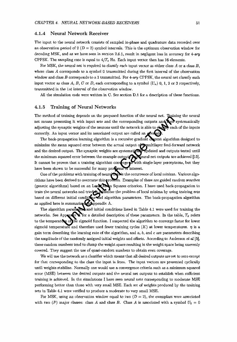
CHAPTER 4. NEURAL NETWORK-BASED RECEIVERS 51
4.1.4 Neural Network Receiver
The input to the neural network consists of sampled in-phase and quadrature data recorded over
an observation period of 2 (D = 2) symbol intervals. This is the optimum observation window for
decoding MSK, and as we have seen in section 2.6.1, result in negligent loss in accuracy for 4-ary
CPFSK. The sampling rate is equal to 4/Ts Hz. Each input vector then has 16 elements.
For MSK, the neural net is required to classify each input vector as either class A or a class B,
where class A corresponds to a symbol 0 transmitted during the first interval of the observation
window and class B corresponds to a 1 transmitted. For 4-ary CPFSK, the neural net classify each
input vector as class A, B, C or D, each corresponding to a symbol (Un) 0, 1, 2 or 3 respectively,
transmitted in the 1st interval of the observation window.
All the simulation code were written in C. See section D.1 for a description of these functions.
4.1.5 Training of Neural Networks
The method of training depends on the proposed function of the neural net. Training the neural
net means presenting it with input sets and the corresponding outputs and then systematically
adjusting the synaptic weights of the neurons until the network is able to classify each of the inputs
correctly. An input vector and its associated output are called an exemplar. The back-propagation learning algOrithm is a recursive gradient descent algorithm designed to
minimize the mean squared error between the actual output of a multilayer feed-forward network
and the desired output. The synaptic weights are systematically updated and outputs tested until
the minimum squared error between the example outputs and neural net outputs are achieved [15].
It cannot be proven that a training algorithm converge as with single-layer perceptrons, but they
have been shown to be successful for many problems of interest. One of the problems with training of neural nets is the occurrence of local minima. Various algo
rithms have been derived to overcome this problem. Examples of these are guided random searches
(genetic algorithms) based on an Least Mean Squares criterion. I have used back-propagation to
train the neural networks and tried to minimize the problem of local minima by using training sets
based on different initial conditions and algorithm parameters. The back-propagation algorithm
as applied here is summarized in appendix A.
The algorithm parameters and initial conditions listed in Table 4.1 were used for training the
networks. See Appendix A for a detailed description of these parameters. In the table, Tz refers
to the temperature of the sigmoid function. I suspected the algorithm to converge faster for lower
sigmoid temperature and therefore used fewer training cycles (K) at lower temperatures. 1] is a
gain term describing the learning rate of the algOrithm, and a, b, and c are parameters describing
the amplitude of the randomly assigned initial weights and offsets. According to Anderson et al [5], these random numbers tend to clump the weight space resulting in the weight space being unevenly
covered. They suggest the use of quasi-random numbers to obtain even coverage.
We will use the network as a classifier which means that all desired outputs are set to zero except for that corresponding to the class the input is from. The input vectors are presented cyclically
until weights stabilize. Normally one would use a convergence criteria such as a minimum squared error (MSE) between the desired outputs and the neural net outputs to establish when sufficient
training is achieved. In the simulations I have seen neural nets corresponding to moderate MSE
performing better than those with very small MSE. Each set of weights produced by the training sets in Table 4.1 were verified to produce a moderate to very small MSE.
For MSK, using an observation window equal to two (D = 2), the exemplars were associated
with two (P) major classes: class A and class B. Class A is associated with a symbol Ua = 0
Univers
ity of
Cap
e Tow
n
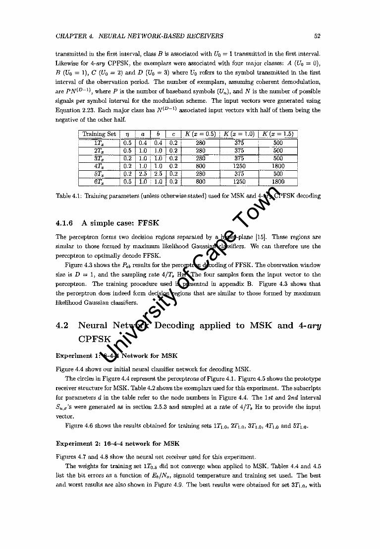
CHAPTER 4. NEURAL NETWORK-BASED RECENERS 52
transmitted in the first interval, class B is associated with Uo 1 transmitted in the first interval.
Likewise for 4-ary CPFSK, the exemplars were associated with four major classes: A (Uo = 0),
B (Uo = 1), C (Uo 2) and D (Uo = 3) where Uo refers to the symbol transmitted in the first
interval of the observation period. The number of exemplars, assuming coherent demodulation,
are PN(D-l), where P is the number of baseband symbols (Un), and N is the number of possible
signals per symbol interval for the modulation scheme. The input vectors were generated using
Equation 2.23. Each major class has N(D-I) associated input vectors with half of them being the
negative of the other half.
I Training Set I 11 a I b elK (x = 0.5) I K (x = 1.0) I K (x = 1.5) IT", 0.5 0.4 0.4 0.2 280 375 500 2T", 0.5 1.0 1.0 0.2 280 375 500 3T", 0.2 LOm 0.2 280 375 500 4T", 0.2 1.0 0.2 800 1250 1800 5T", 0.2 2.5 2.5 0.2 280 375 500 6T", 0.5 1.0 1.0 0.2 800 1250 1800 I
Table 4.1: Training parameters (unless otherwise stated) used for MSK and 4-ary CPFSK decoding
4.1.6 A simple case: FFSK
The perceptron forms two decision regions separated by a hyper-plane [15]. These regions are
similar to those formed by maximum likelihood Gaussian classifiers. We can therefore use the
percept ron to optimally decode FFSK.
Figure 4.3 shows the Peb results for the percept ron decoding of FFSK. The observation window
size is D == 1, and the sampling rate 4/Ts Hz. The four samples form the input vector to the
perceptron. The training procedure used is presented in appendix B. Figure 4.3 shows that
the perceptron does indeed form decision regions that are similar to those formed by maximum
likelihood Gaussian classifiers.
4.2 Neural Network Decoding applied to MSK and 4-ary
CPFSK
Experiment 1: 8-4-4 Network for MSK
Figure 4.4 shows our initial neural classifier network for decoding MSK.
The circles in Figure 4.4 represent the perceptrons of Figure 4.1. Figure 4.5 shows the prototype
receiver structure for MSK. Table 4.2 shows the exemplars used for this experiment. The subscripts
for parameters d in the table refer to the node numbers in Figure 4.4. The 1st and 2nd interval
S .. ,u's were generated as in section 2.5.3 and sampled at a rate of 4/Ts Hz to provide the input
vector.
Figure 4.6 shows the results obtained for training sets ITl.o, 2Tl.o, 3Tl.o, 4Tl.o and 5Tl.o.
Experiment 2: 16-4-4 network for MSK
Figures 4.7 and 4.8 show the neural net receiver used for this experiment.
The weights for training set ITo.s did not converge when applied to MSK. Tables 4.4 and 4.5
list the bit errors as a function of Eb/No, sigmoid temperature and training set used. The best
and worst results are also shown in Figure 4.9. The best results were obtained for set 3Tl.O, with
Univers
ity of
Cap
e Tow
n

CHAPTER 4. NEURAL NETWORK-BASED RECENERS 53
Ic-07 +-~~..-,.+-.,......,.~.,.......-I-.,.......~~-+~~...,.....,--+-~~""":"',., o 3 6 9 12 15
Figure 4.3: Perceptron BER results for FFSK
Table 4.2: Exemplars for MSK training, experiment 1
Univers
ity of
Cap
e Tow
n
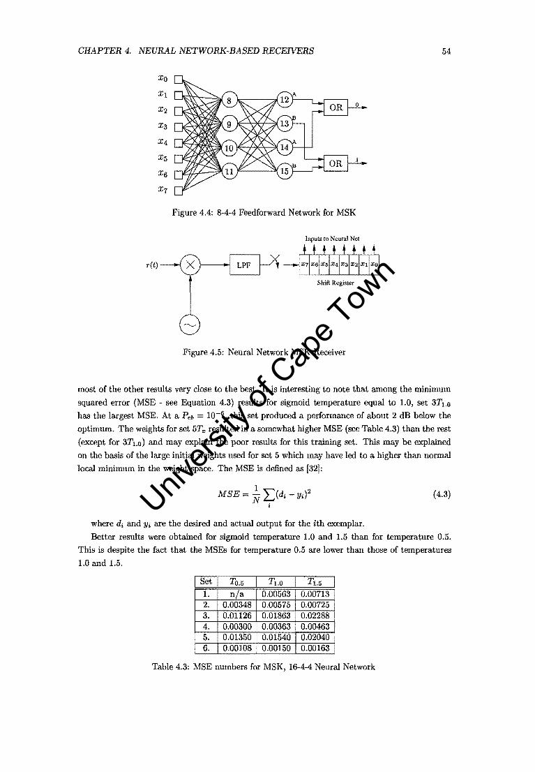
CHAPTER 4. NEURAL NETWORK-BASED RECEIVERS 54
Figure 4.4: 8-4-4 Feedforward Network for MSK
Inputs to Neural Net
ret}
Figure 4.5: Neural Network MSK Receiver
most of the other results very close to the best. It is interesting to note that among the minimum
squared error (MSE - see Equation 4.3) results for sigmoid temperature equal to 1.0, set 3T1.0
has the largest MSE. At a Peb = 10-6 , this set produced a performance of about 2 dB below the
optimum. The weights for set 5T", resulted in a somewhat higher MSE (see Table 4.3) than the rest
(except for 3T1.O) and may explain the poor results for this training set. This may be explained
on the basis of the large initial weights used for set 5 which may have led to a higher than normal
local minimum in the weight space. The MSE is defined as [32]:
1" 2 MSE = N L.J(di - y;) i
where di and Yi are the desired and actual output for the ith exemplar.
(4.3)
Better results were obtained for sigmoid temperature 1.0 and 1.5 than for temperature 0.5.
This is despite the fact that the MSEs for temperature 0.5 are lower than those of temperatures
1.0 and 1.5.
Set To.5 71.0 71.5
1. nla 0.00563 0.00713 • 2. 0.00348 0.00575 0.00725 i
3. 0.01126 0.01863 0.02288 !
4. 0.00300 0.00363 0.00463 5. 0.01350 0.01540 0.02040 6. 0.00108 0.00150 0.00163
Table 4.3: MSE numbers for MSK, 16-4-4 Neural Network
Univers
ity of
Cap
e Tow
n

CHAPTER 4. NEURAL NETWORK-BASED RECENERS 55
Figure 4.6: BER results for MSK using 8-4-4 Neural Network
I Test I EblNo , dB I ITo 5 I 1T10 I 1T15 I 2To 5 I 2T10 I 2T15 I 3To 5 I 3T10 I 3T15 I bits 1. 12.04 n/a 7 7 6 2 3 8 2 2 50 Ok 2. 10.45 n/a 57 47 60 26 25 51 21 23 50 Ok 3. 7.95 n/a 217 197 240 166 166 241 136 147 lOOk
Table 4.4: 16-4-4 Neural Network MSK Bit Errors
I Test I EblNo , dB I 4To 5 I 4T10 I 4T15 I 5To 5 I 5T10 I 5T15 I 6To 5 I 6T10 I 6T15 I bits 4. 12.04 4 2 4 8894 1004 816 5 3 4 500k 5. 10.45 57 27 26 18057 2778 2388 65 34 31 500k 6. 7.95 240 168 173 7832 1759 1557 250 186 172 lOOk
Table 4.5: 16-4-4 Neural Network MSK Bit Errors
Univers
ity of
Cap
e Tow
n
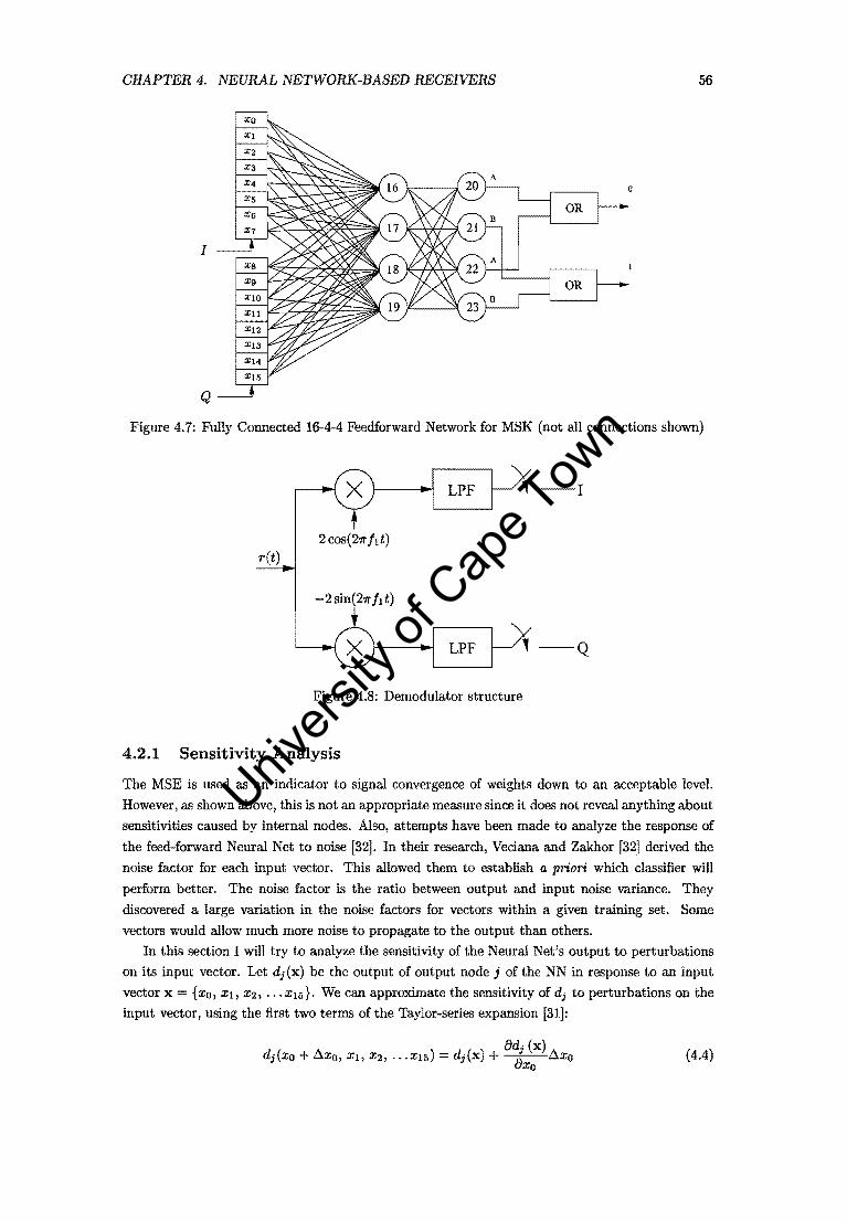
CHAPTER 4. NEURAL NETWORK-BASED RECEIVERS 56
I
Q
Figure 4.7: Fully Connected 16-4-4 Feedforward Network for MSK (not all connections shown)
I
2cos(21rflt) ret)
Figure 4.8: Demodulator structure
4.2.1 Sensitivity Analysis
The MSE is used as an indicator to signal convergence of weights down to an acceptable level.
However, as shown above, this is not an appropriate measure since it does not reveal anything about
sensitivities caused by internal nodes. Also, attempts have been made to analyze the response of
the feed-forward Neural Net to noise [32]. In their research, Veciana and Zakhor [32] derived the
noise factor for each input vector. This allowed them to establish a priori which classifier will
perform better. The noise factor is the ratio between output and input noise variance. They
discovered a large variation in the noise factors for vectors within a given training set. Some
vectors would allow much more noise to propagate to the output than others.
In this section I will try to analyze the sensitivity of the Neural Net's output to perturbations
on its input vector. Let dj(x) be the output of output node j of the NN in response to an input
vector x = {xo, Xl, X2, .•• X15}. We can approximate the sensitivity of dj to perturbations on the
input vector, using the first two terms of the Taylor-series expansion [31]:
d () adj (x) A
j X + -a--UXo Xo
(4.4)
Univers
ity of
Cap
e Tow
n

CHAPTER 4. NEURAL NETWORK-BASED RECEIVERS 57
le+OO
Ie-Ol -......
, '. STO.5
'" '"
, '. "'" , ......... ~ "-le-02
"" STl.o
le-03 \ ~ ..•....
STu
, I~ "- ..
"-.'\ ... .. le-04
\ ~\ -,,\ FSK Ie-OS
MSK , 3TI.o '. , '.
le-06 \
Ie-07 o 3 12 IS
Figure 4.9: Best and worst BER results for MSK using 16-4-4 Neural Net
Solving for g~~ and using the central-difference quotient to approximate the derivatives result
in:
(4.5)
I used this equation to calculate the sensitivity matrix. It should be noted that ifAxo is too
large, the difference quotient is normally a poor approximation of the derivative. The sensitivity
matrix consist of 8dj (x) /8xo values for all output nodes (all1's). The matrix has one sensitivity
number for each element of the input vector x, for all valid input vectors. Each element in each
input vector is perturbed by AXi = Xi/10. Table 4.6 shows the maximum values among the
elements of the sensitivity matrixes for each training set. See appendix C for a listing of two of
these matrixes (5To.5 and 3T1.o),
I Training Set To 5 IT", nla 0.0926 0.0577
I 2T:t 0.1766 0.1293 0.0459 3T:t 0.2091 0.1663 0.0665 4T:z: 0.1807 0.1216 0.0546 5T:z: 0.3883 0.2133 0.2680 .
I 6T:t 0.1420 0.0901 0.0429 •
Table 4.6: Maximum sensitivity numbers parameters for 16-4-4 Neural Net for MSK
Although using only the maximum element of the matrix is not an appropriate criterion (some
measure need to be derived that take into account all the sensitivities) to describe the a priori
performance of the network, it does show better agreement between actual performance and pre
dicted performance of the network than does the MSE. Figure 4.10 shows a comparison between
Univers
ity of
Cap
e Tow
n
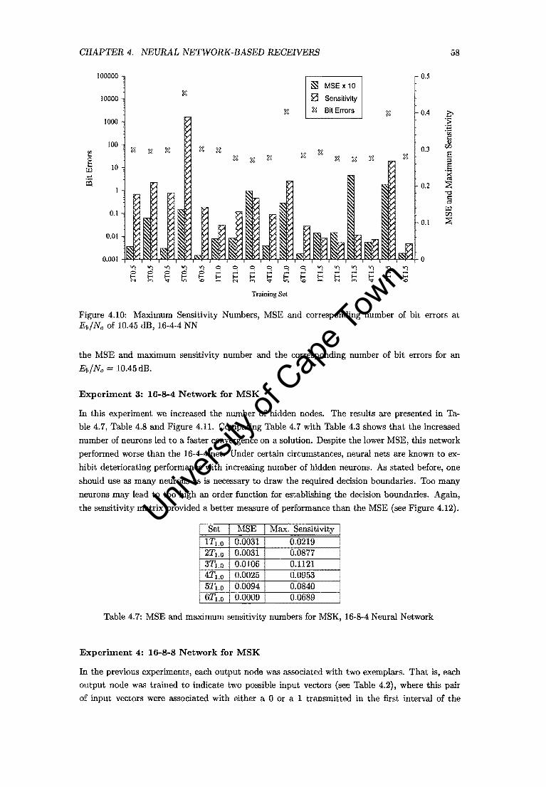
CHAPTER 4. NEURAL NETWORK-BASED RECENERS 58
100000 0.5
~ MSE X 10
10000 1:S 0 Sensitivity
~ ~ Bit Errors t:: 0.4 1000
100 til 0.3 .... E 10 Ul .....
05 0.2
0.1 0.1
0.01
0.001 0
'" '" VI '" '" ~ ~ ~ ~ ~ ~ '" '" '" '" '" '" 0 0 0 0 0 1= E E= 1= ~ 1= Eo< Eo< t; Eo< Eo< t: Eo< Eo< Eo< Eo< Eo< N ..... '" -.0 N ..... .... '" -.0 N ..... ..... >0
Training Set
Figure 4.10: Maximum Sensitivity Numbers, MSE and corresponding number of bit errors at Eb/No of 10.45 dB, 16-4-4 NN
the MSE and maximum sensitivity number and the corresponding number of bit errors for an
Eo/No = 10.45 dB.
Experiment 3: 16-8-4 Network for MSK
In this experiment we increased the number of hidden nodes. The results are presented in Ta
ble 4.7, Table 4.8 and Figure 4.11. Comparing Table 4.7 with Table 4.3 shows that the increased
number of neurons led to a faster convergence on a solution. Despite the lower MSE, this network
performed worse than the 16-4-4 net. Under certain circumstances, neural nets are known to ex
hibit deteriorating performance with increasing number of hidden neurons. As stated before, one
should use as many neurons as is necessary to draw the required decision boundaries. Too many
neurons may lead to too high an order function for establishing the decision boundaries. Again,
the sensitivity matrix provided a better measure of performance than the MSE (see Figure 4.12).
I Set I MSE I Max. Sensitivity I
~.O 0.0031 0.0219 2Tl.o 0.0031 0.0877 3T1.o 0.0106 0.1121 4T1.o 0.0025 0.0953
•
I 5Tl.o 0.0094 0.0840 • 6T1.o 0.0009 0.0689
Table 4.7: MSE and maximum sensitivity numbers for MSK, 16-8-4 Neural Network
Experiment 4: 16-8-8 Network for MSK
In the previous experiments, each output node was associated with two exemplars. That is, each
output node was trained to indicate two possible input vectors (see Table 4.2), where this pair
of input vectors were associated with either a 0 or a 1 transmitted in the first interval of the
Univers
ity of
Cap
e Tow
n
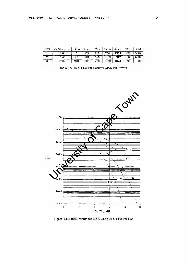
CHAPTER 4. NEURAL NETWORK-BASED RECEIVERS 59
I Test I Eb/No ,dB 11T1 o I 2T10 I 3T1 o I 4T10 I 5T1 o 16TlO I bits I .
1. 12.04 5 121 111 254 1359 220 500k I I 2. 10.45 73 704 655 1079 3312 1006 500k I
I 3. 7.95 240 803 770 1032 1874 991 lOOk·
Table 4.8: 16-8-4 Neural Network MSK Bit Errors
] e-G7 -r-.~~~j--,-~~-'-+~..--r-.....-.-+-~~..--r--j--.~~.-'-.,'" -, o 3 6 9 12 15
Figure 4.11: BER results for MSK using 16-8-4 Neural Net
Univers
ity of
Cap
e Tow
n

CHAPTER 4. NEURAL NETWORK-BASED RECEIVERS
10000
1000
100
10
OJ
0.01
0.001
Training Set
l§:I MSEx10
o Sensitivity
n Bit Errors
60
0.5
Figure 4.12: Maximum Sensitivity Numbers, MSE and corresponding number of bit errors at Eb/No of 10.45 dB, 16-8-4 NN
observation period. In this experiment we assigned each exemplar an unique output node and we
expect to see better results. We do this experiment using training sets 3To.5, 3Tl.o and 3T1.5, but
now with varying number of training cycles to ensure that the MSE is between 0.0007 and 0.0004
(except for set 3Tl.Ob). The results are shown in Tables 4.10 and 4.9. The maximum sensitivity
numbers does not show very good agreement with bit error performance. This may indicate that
the complete sensitivity matrix should be used as a figure of merit rather than the maximum
sensitivity number.
The error rate for this network is surprisingly higher than .the 16-4-4 network.
Parameter 3To5 3Tl 0 I 3Tl Ob I 3T1 5
MSE 0.000660 0.000515 0.Q1380 0.000493 Max. Sensitivity 0.0251 0.0652 0.0561 0.0263 Training Cycles 3000 14000 4000 15000
Table 4.9: 16-8-8 Neural Network for MSK showing MSE, training cycles and maximum sensitivity numbers
I Test I Eb/No , dB I 3To 5 I 3T10 I 3T10b I 3T15 I bits 1. 12.04 57 48 38 97 500k 2. 10.45 373 256 299 554 500k 3. 7.95 621 426 525 695 lOOk
Table 4.10: 16-8-8 Neural Network MSK Bit Errors
Experiment 5: 16-16-8 Network for MSK
In this experiment we increased the number of hidden neurons. Tables 4.11 and 4.12 show the
results for training set 3Tl.o. Increasing the number of hidden neurons improved the performance
with respect to the 16-8-8 net, but performance is still disappointing compared to the simple 16-4-4
Univers
ity of
Cap
e Tow
n

CHAPTER 4. NEURAL NETWORK-BASED RECENERS 61
network.
Parameter 3Tl 0
MSE 0.000266 • Max. Sensitivity 0.0346 I 'fraining Cycles 13000 I
Table 4.11: 16-16-8 Neural Network for MSK showing MSE, training cycles and maximum sensitivity numbers
I Test I EblNo ,dB I 3Tlo I bits 1. 12.04 12 500k 2. 10.45 153 SOOk 3. 7.95 461 lOOk
Table 4.12: 16-16-8 Neural Network MSK Bit Errors
Experiment 6: 16-16-8 Network for 4-a'1'Y CPFSK
The results of this experiment were disappointing. Table 4.14 and Tables 4.15, 4.16 and 4.17 show
that some decoding is performed, but that the error rates are completely unacceptable. The same
decoder concept was used as before and as shown in Figure 4.7. This bad performance can be
attributed to either too many (over-fitting of the decision boundaries) or too few hidden neurons,
and lor to the occurrence of a local minimum in the weight space. I did not perform a sensitivity
analysis for each training set. The maximum sensitivity numbers for set 1To.s and 6T1.5 were
0.4709 and 0.2812 respectively. This contradicts our previous success, but as stated before, the
complete sensitivity matrix should be studied instead of one number only. Another contributing
factor to the poor performance of this net may be due to the way the exemplars were set up.
Table 4.13 list the class A exemplars. Each output node were required to identify eight different
input vectors. This setup was applied to MSK and a feasible explanation for its success is that the
2 input vectors associated with each output node are coincidentally on the same side of a decision
boundary for that specific net. The eight input vectors associated with each output node may be
on different sides of a decision boundary for this specific net.
4.2.2 Performance Analysis and Summary
With respect to sigmoid temperature, the best results were obtained for values between T = 1.0
and T = 1.5. One might expect a net to perform better with hidden nodes saturated and having
higher temperatures since this would indicate lower hidden sensitivities.
The MSE criteria is only a measure of how close the output nodes are to required values
when presented with a specific input vector. It does not reveal any hidden sensitivities. The
sensitivity matrix should be used as a convergence measure in training and to evaluate a network's
performance under noisy circumstances.
The 16-4-4 net for MSK network performed surprisingly better thart the nets for which each
output node were required to identify an unique input vector. I cannot explain this, except than
to say that the input vector pair associated with eaclt output node for the 16-4-4 net may be on
the same side of some decision boundary.
Comparing the results of the 16-8-8 and the 16-16-8 networks for MSK show that increasing the
number of hidden nodes improve the performance. This tendency was also noticed by de Veciana
Univers
ity of
Cap
e Tow
n

CHAPTER 4. NEURAL NETWORK-BASED RECEIVERS 62
Interval > 1st 2nd output node class setting
An Sao So,o di = 0, d33 = 1 Al So,o Sl,O di :::: 0, d33 = 1 A2 Soo S2,0 d;:::: 0, d33 = 1 As So,o~ di = 0, d33 :::: 1 ~ SO,l 1 di = 0, d33 = 1 A5 SO,l Sl1 di 0, d33 = 1 A6 SO,l S2,1 di = 0, d33 = 1 A7 SO,l 83,1 d; = 0, d33 = 1 As 80,2 8 0,2 d; = 0, d37 = 1 As 80,2 81,2 d; :::: 0, da7 = 1 AlO 80,2 82,2 di 0, d37 :::: 1 : All 8 0,2 8 3,2 d; = 0, d37 :::: 1 Al2 8 0,3 8 0,3 di :::: 0, d37 :::: 1 Al3
~: 81,3 di :::: 0, d37 = 1
A14 S2,3 d; = 0, d37 = 1 !
A15 0,3 83,3 d; :::: 0, d37 :::: 1 •
Table 4.13: Exemplars for 4-ary CPFSK training (only class A shown here)
~ TO.5 Tl.O T1.5
0.00136 0.00157 0.00215 0.06343 0.00218 0.00485
3. 0.00435 0.00688 0.00675 4. 0.00127 0.00081 0.00096 5 . 0.13124 0.06799 0.00773
• 6. 0.06283 0.00036 0.000472
Table 4.14: 16-16-8 Neural Network for 4-ary CPFSK, MSE
[ Test [ Eo/No, dB [ ITo 5 [ ITlO [ IT15 [ 2To 5 [ 2TlO [2T15 bits 1. 17.00 399 1970 4207 7462 5005 3363 lOOk i
2. 13.47 3077 7588 8167 10925 9232 10988 lOOk! 3. 10.97 8013 15235 14969 16520 15655 19326 lOOk I 4. 7.45 20904 30493 30033 29518 29751 22867 lOOk I
Table 4.15: 16-16-8 Neural Network 4-ary CPFSK Bit Errors
[ Test [ Eb / No ,dB [ 3To 5 [ 3TI 0 [ 3Tl 5 [ 4To 5 [ 4TI 0 [ 4Tl 5 bits 5. 17.00 I 4410 1730 1915 4848 1215 1633 lOOk 6. 13.47 I 11161 7035 7803 11607 6477 8109 lOOk 7. 10.9( I J.9367 14883 15573 19652 14475 16681 lOOk 8. 7.45 134494 30036 30942 34578 30151 32165 lOOk
Table 4.16: 16-16-8 Neural Network 4-ary CPFSK Bit Errors
[ Test [ Eo/No, dB [ 5To 5 [ 5TIO I 5TI5 [ 6To 5 I 6Tlo [ 6Tl 5 bits 9. 17.00 13289 7495 3301 7559 2309 I 2969 lOOk I 10. 13.47 16538 11785 10582 10559 6669 I 9733 lOOk. 11. 10.97 21596 18419 18877 15793 ~49 lOOk I 12. 7.45 33310 32534 33650 28574 2 33185 lOOk I
Table 4.17: 16-16-8 Neural Network 4-ary CPFSK Bit Errors
Univers
ity of
Cap
e Tow
n

CHAPTER 4. NEURAL NETWORK-BASED RECEIVERS 63
le+OO
~ 5TO.5 ..... ~
Ie-OJ ............ -~ ~
4TU
'. "'. "
,
Ie-02 ..... ,. ITO~4
' . Ie-03 ..
Ie-04
Ie-05 4-aryCPFSK
Je-06 ~\
Ie-07 2 5 8 11 14 17
Figure 4.13: Best and worst BER results for 4-ary CPFSK
and Zakhor [32], and I agree with their rule of thumb for best performance: have approximately
as many hidden nodes as input nodes.
The occurrence of local minima may always be a problem. One possible way of minimizing
the phenomenon of local minima may be to apply a guided random search (genetic algorithm)
for optimum weights. Otherwise, my suggestion is to keep with the standard back-propagation
training algorithm (except than to integrate the sensitivity matrix into the convergence criterion)
and do manual guided searches. This may include:
1. Lowering the gain term 1'/ in the back-propagation training algorithm
2. Performing training runs starting with many different sets of initial random weights, and
3. Changing the order in which the inputs vectors are presented
Further options for future research may include using a larger observation window and a higher
sampling rate. It could also be that the neural nets applied in this research is not able to define
the complex decision boundaries required by convolutional codes. More emphasis should be placed
on understanding the boundaries formed by these neural nets. A final note is that nearly all the
symbol errors generated by the neural nets occurred as single burst length errors. This was not
the case with the Fano algorithm where nearly all the symbol errors occurred as burst errors of
length 2, whereas about 30 to 40 percent of the errors made by the Viterbi decoder were single symbol errors.
Wicker and Wang [33] designed a neural network that implements the Viterbi algorithm using
analog artificial neurons. The performance of this network matches the ideal Viterbi algorithm
since it is basically a "neuralized" version of the Viterbi algorithm. They point out that the code
Univers
ity of
Cap
e Tow
n
CHAPTER 4. NEURAL NETWORK-BASED RECEIVERS 64
words of conventional pattern recognition problems form a vector space over a finite field, whereas
the algebraic properties of practical block codes and convolutional codes may introduce additional
structure. This type of artificial neural net decoder is superior in terms of speed and is better
suited for VLSI implementation than current decoder designs.
4.2.3 Complexity
Veciana and Zakhor [321 provide an arithmetic complexity comparison between conventional re
ceivers and NN based receivers. Their arithmetic comparison is based on a digital implementation
and in terms of number of addition, multiply, table lookup, compare and select operations per
formed per symbol interval for each receiver. The conclusion is that the NN numerical complexity
exceeds that of a conventional Viterbi implementation by a factor of about 3 (Wicker's neural
net decoder as discussed above is excluded from these calculations). Whereas the Viterbi decoder
requires substantial RAM and some ROM, the NN requires virtually no RAM but substantial
ROM.
Univers
ity of
Cap
e Tow
n
Chapter 5
Conclusioll
5.1 Summary
5.1.1 The Fano Algorithm
This thesis contains new results on the subject of two methods for decoding the continuous-phase
modulated signal. Neither of these two techniques have been effectively implemented in practice
and there is a proportional paucity in research results, especially for the Fano decoder.
We applied the Fano decoder to 4-ary CPFSK with the purpose of investigating firstly, its
suitability as decoder for CPM in general, and secondly, the possibility of it providing a less
complex decoder structure. The second technique, namely the neural network decoder, was in
addition to 4-ary CPFSK also applied to MSK.
We confirmed through simulation that the Fano decoder approaches the bit error rate perfor
mance of the optimum decoder for high signal-to-noise ratios.
The major problem at lower Eb/No seems to be that of undetected re-merging paths. The
re-merging of paths causes error bursts of length 2. One important conclusion is that catastrophic
events are, within a fairly large range of threshold and slope parameters, not the handicap we
anticipated it to be. Of special importance is the results on the percentage of time the decoder
spent looking back and actually moving back as a function of Eb/No, Fano threshold, and Fano
slope parameters. We showed that at Eb/No = 13.1 dB where bit error rate performance is still
acceptable, look-backs amount to about 5 percent of symbols received and move-backs amount to
about 2 percent.
One disadvantage is the decoding delay with respect to the Viterbi decoder. This delay also
determines the amount of memory required since all metric values need to be stored up to this
depth. This delay is a function of the maximum depth reached in looking back (values in brackets)
for Eb/No= 16 dB (3), 13.1 dB (5) and 8.4 dB (12). However, it is not certain how the decoding
delay of the Fano algorithm relative to those of the Viterbi will change for schemes with longer
constraint length. It may well be that the decoding delay compared to those of the Viterbi decoder
decreases with increase in constraint length.
The Fano algorithm was substantially more complex to implement in software than the Viterbi
algorithm, but it remains to be investigated how the respective complexities of the hardware
implementations compare with each other.
65
Univers
ity of
Cap
e Tow
n

CHAPTER 5. CONCLUSION 66
5.1.2 The Neural Net Decoder
The neural network decoder take as input samples of the baseband in-phase and quadrature wave
forms instead of the traditional approach of using the output from a set of matched filters as input
for the neural network. Our bit error rate results were disappointing and confirms the results of
other researchers.
We presented a method for determining the hidden sensitivities of the neural network which
gives an a priori performance indication. This method should rather be used as a convergence
measure in training and to evaluate a network's performance under noisy circumstances.
We concluded that the decision regions required by convolutional codes have additional struc
ture which is not adequately represented by the decision boundaries formed by feed-forward neural
nets. The NN's numerical complexity exceeds that of the conventional Viterbi implementation by
a factor of about 3.
5.2 Future Work
Of the two techniques applied, the Fano algorithm turned out to be the most promising. Future
research on the subject of Fano decoders may be divided in two parts:
1. The research should be repeated for a modulation scheme with larger constraint length in
order to establish the effect off constraint length on decoding delay and consequently memory
usage. To what extend can the decoding delay be reduced for the algorithm to still function
with acceptable performance?
2. Transforming the Fano algorithm into a simplified hardware implementation and doing a
resource comparison with the Viterbi implementation.
Suggested future research on the neural network decoder may include the following:
1. A criteria which indicate a priori performance based on hidden neuron sensitivities should
be investigated.
2. Finally, the additional structure in the decision regions required by convolutional codes need
to be investigated for better understanding and possible modification to the neural net struc
ture. Univers
ity of
Cap
e Tow
n

Appendix A
The Back-propagation Neural Net
Training Algorithm
The back-propagation learning algoritlnn is a recursive gradient algoritlnn designed to minimize
the mean squared error between the actual output of a multilayer feed-forward network and the
desired output. The algoritlnn as presented here is from [15], but with slightly different notation.
We assume a sigmoidal activation function:
1 fact(a) = ---,:-
1+ Step 1. Initialize weights and offsets
Set all synaptic weights and node offsets to small random values.
The weights were set upon initialization using the following C equations:
1st layer: wt[i] = a * (1.0 * randO/RAND _MAX - 0.5)
2nd layer: w2[i] = b * (1.0 HandO/RAND _MAX - 0.5)
offsets: o!!set[i] c * (1.0 HandO/RAND _MAX - 0.5);
Step 2. Present input and desired outputs
(A.l)
Present a continuous valued input vector xo, Xl, .• • XN-l and specify the desired out
puts do, dl, ... dM-l. We will use the network as a classifier which means that all
desired outputs are set to zero except for that corresponding to the class the input is
from. The input samples used as training sets are presented cyclically until weights
stabilize. For MSK, using an observation period equal to two, the training sets were
associated with two major classes: class A and class B. Class A is associated with an
Uo = 0 transmitted in the first interval, class B is associated with Uo 1 transmitted
in the first interval. Likewise for 4-ary CPFSK, the training sets were associated with
four major classes: A (UO = 0), B (Uo = I), C (Uo = 2) and D (Uo = 3) where Uo refer here to the symbol transmitted in the first interval of the observation period.
Step 3. Calculate actual outputs
Calculate outputs Yo, yl, ... YM-I·
Step 4. Adapt weights
Use a recursive procedure starting at the output nodes and working back to the first
hidden layer. Adjust the synaptic weights according to
67
Univers
ity of
Cap
e Tow
n

APPENDIX A. THE BACK-PROPAGATION NEURAL NET TRAINING ALGORITHM 68
xi is either the output of node i or is an input, 11 is a gain term, and OJ is an error term
for node j. If node j is an output node, then
where dj is the desired output of node j, and Yj is the actual output.
If node j is an internal hidden node, then
OJ = xj(l- xj) L OkWjk , k
where k is over all nodes in the layers above node j. Internal node thresholds are
adapted in a similar manner by assuming they are connection weights on links from
auxiliary constant-valued inputs.
Step 5. Repeat (K times) by going to step 2
Univers
ity of
Cap
e Tow
n
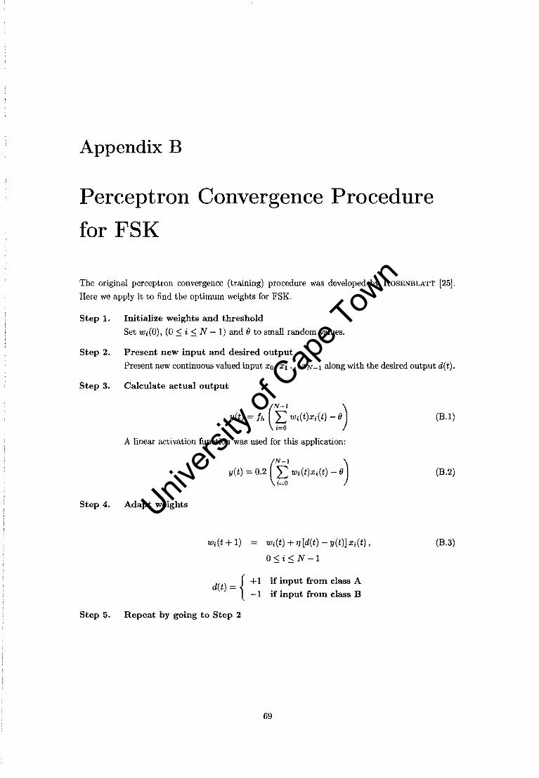
Appendix B
Percept ron Convergence Procedure
for FSK
The original perceptron convergence (training) procedure was developed by ROSENBLATl' [25J.
Here we apply it to find the optimum weights for FSK.
Step 1. Initialize weights and threshold
Set Wi(O), (0 S; i S; N - 1) and 8 to small random values.
Step 2. Present new input and desired output
Present new continuous valued input xo, Xl .•. xN-I along with the desired output d(t).
Step 3. Calculate actual output
(
N-I ) yet) = fh ~ Wi(t)X;(t) - 8
A linear activation function was used for this application:
Step 4. Adapt weights
(
N-l ) yet) = 0.2 ~ Wi(t)Xi(t) - 8
Wi(t) + r} [d(t) - yet)] x;(t) ,
OS;iS;N 1
d(t) = {+1 if input from class A -1 if input from class B
Step 5. Repeat by going to Step 2
69
(B.1)
(B.2)
(B.3)
Univers
ity of
Cap
e Tow
n

Appendix C
Sensitivity Matrix for 16-4-4 NN
MSK
C.l Sensitivity matrix for training set 5To.5
weights16-4-4
Sensitivity analysis: dx = 0.1000
ddj/dxO, class 0: -0.0447 0.0682 -0.0004 -0.0623
ddj/dx1, class 0: -0.0910 0.0381 0.0000 -0.0335
ddj/dx2, class = 0 : 0.0553 -0.0298 -0.0000 0.0173
ddj/dx3, class = 0 : 0.0006 0.0325 -0.0001 -0.0130
ddj/ dx4, class = 0 : 0.1007 -0.0489 0.0001 0.0353
ddj/dx5, class = 0 : 0.0313 -0.0206 -0.0001 0.0123
ddj/dx6, class 0: 0.0487 -0.0548 0.0002 0.0459
ddj/dx7, class = 0 : -0.0497 0.0415 -0.0002 -0.0503
ddj/dx8, class = 0 : 0.0000 0.0000 0.0000 0.0000
ddj/dx9, class = 0 : 0.0000 0.0000 0.0000 0.0000
ddj/dx10, class = 0 : 0.0000 0.0000 0.0000 0.0000
ddj/dxll, class = 0 : 0.0000 0.0000 0.0000 0.0000
ddj/dx12, class 0: 0.0000 0.0000 0.0000 0.0000
ddj/dx13, class 0: 0.0000 0.0000 0.0000 0.0000
ddj/ dx14, class = 0 : 0.0000 0.0000 0.0000 0.0000
ddj/ dx15, class = 0 : 0.0000 0.0000 0.0000 0.0000
ddj/dxO, class = 1 : -0.0121 0.0344 -0.0004 -0.0058
ddj/dxl, class 1 : -0.0097 -0.0028 0.0001 0.0006
ddj/ dx2, class 1 : 0.0041 0.0030 -0.0001 -0.0008
ddj/dx3, class 1 : 0.0048 0.0007 0.0000 0.0004
ddj/dx4, class = 1 : 0.0108 -0.0085 0.0001 0.0013
ddj/dx5, class = 1 : 0.0000 0.0000 0.0000 0.0000 ddj/dx6, class = 1 : -0.0086 0.0198 -0.0002 -0.0031
ddj/dx7, class 1 : 0.0095 -0.0173 0.0002 0.0026
ddj/dx8, class 1 : 0.0000 0.0000 0.0000 0.0000 ddj/dx9, class = 1 : 0.0000 0.0000 0.0000 0.0000
ddj/ dxlO, class = 1 : 0.0000 0.0000 0.0000 0.0000
ddj/dxll, class = 1 : 0.0000 0.0000 0.0000 0.0000
ddj/ dx12, class = 1 : -0.0032 -0.0034 0.0001 0.0011
ddj/ dx13, class = 1 : 0.0000 0.0000 0.0000 0.0000
70
Univers
ity of
Cap
e Tow
n

APPENDIX C. SENSITIVITY MATRIX FOR 16-4-4 NN MSK 71
ddj/dx14, class = 1 : -0.0070 0.0146 -0.0002 -0.0030
ddj/dxI5, class = 1 : 0.0000 0.0000 0.0000 0.0000
ddj/dxO, class 2: 0.0007 -0.0468 0.0557 0.3176
ddj/dx1, class 2: 0.0020 -0.0185 -0.0025 0.2723
ddj/dx2, class 2 : -0.0012 0.0141 0.0010 -0.1981
ddj/dx3, class = 2 : -0.0002 -0.0191 0.0168 0.1229
ddj/dx4, class = 2 : -0.0022 0.0220 -0.0094 -0.3691
ddjfdx5, class = 2 : -0.0006 0.0113 0.0135 -0.0847
ddj/dx6, class = 2 : -0.0009 0.0322 -0.0339 -0.2808
ddj/dx7, class 2: 0.0009 -0.0276 0.0256 0.2052
ddj/dx8, class 2: 0.0000 0.0000 0.0000 0.0000
ddj/dx9, class = 2 : 0.0000 0.0000 0.0000 0.0000
ddj/dx10, class = 2 : 0.0000 0.0000 0.0000 0.0000
ddj/dxll, class = 2 : 0.0000 0.0000 0.0000 0.0000
ddj/dx12, class = 2 : 0.0000 0.0000 0.0000 0.0000
ddj/dxI3, class 2: 0.0000 0.0000 0.0000 0.0000
ddj/dx14, class 2: 0.0000 0.0000 0.0000 0.0000
ddj/ dx15, class 2: 0.0000 0.0000 0.0000 0.0000
ddj/ dxO, class = 3 : 0.0002 -0.0335 0.1455 0.3883
ddj/dxl, class = 3 : 0.0018 -0.0015 -0.0368 0.0844
ddj/dx2, class 3 : -0.0008 0.0018 0.0290 -0.0237
ddj/ dx3, class 3 : -0.0009 -0.0102 0.0107 0.0356
ddj/dx4, class = 3 : -0.0014 0.0051 -0.0145 -0.1665
ddj/dx5, class = 3 : 0.0000 0.0000 0.0000 0.0000
ddj/dx6, class = 3 : 0.0004 -0.0149 0.0746 0.2532
ddj/dx7, class = 3 : -0.0008 0.0126 -0.0609 -0.2757
ddj/dx8, class 3: 0.0000 0.0000 0.0000 0.0000
ddj/dx9, class 3 : 0.0000 0.0000 0.0000 0.0000
ddj/dxlO, class 3: 0.0000 0.0000 0.0000 0.0000
ddj/dxll, class = 3 : 0.0000 0.0000 0.0000 0.0000
ddj/dxI2, class = 3 : 0.0006 -0.0070 -0.0288 0.0532
ddj/dxI3, class = 3 : -0.0005 0.0174 -0.0837 -0.2971
ddj/dx14, class 3 : 0.0006 -0.0039 0.0620 0.1458
ddj/dx15, class 3: 0.0000 0.0000 0.0000 0.0000
ddj/dxO, class 4 : 0.0368 0.0155 -0.0360 -0.0002
ddj/dx1, class = 4 : 0.0000 0.0000 0.0000 0.0000
ddj/dx2, class = 4 : -0.0220 0.0146 0.0167 -0.0001
ddj/dx3, class = 4 : -0.0529 -0.0054 0.0300 -0.0000
ddj/dx4, class 4: -0.0658 0.0102 0.0305 -0.0002
ddj/dx5, class 4 : 0.0227 -0.0062 -0.0054 0.0001
ddj/dx6, class = 4 : 0.0381 0.0289 -0.0360 -0.0002
ddj/dx7, class = 4 : -0.0187 0.0008 0.0256 0.0001
ddj/dx8, class = 4 : 0.0217 0.0239 -0.0061 -0.0000
ddj/dx9, class = 4 : 0.0354 0.0288 -0.0325 -0.0002
ddj/dx10, class = 4 : 0.0046 -0.0006 0.0002 0.0000
ddj/dxll, class 4: 0.0000 0.0000 0.0000 0.0000
ddj/ dx12, class 4: 0.0000 0.0000 0.0000 0.0000
ddj/dx13, class 4: 0.0000 0.0000 0.0000 0.0000
ddj/dx14, class = 4 : 0.0000 0.0000 0.0000 0.0000
ddj/dx15, class = 4 : 0.0000 0.0000 0.0000 0.0000
ddj/dxO, class = 5 : 0.0062 0.0414 -0.0262 -0.0006
Univers
ity of
Cap
e Tow
n
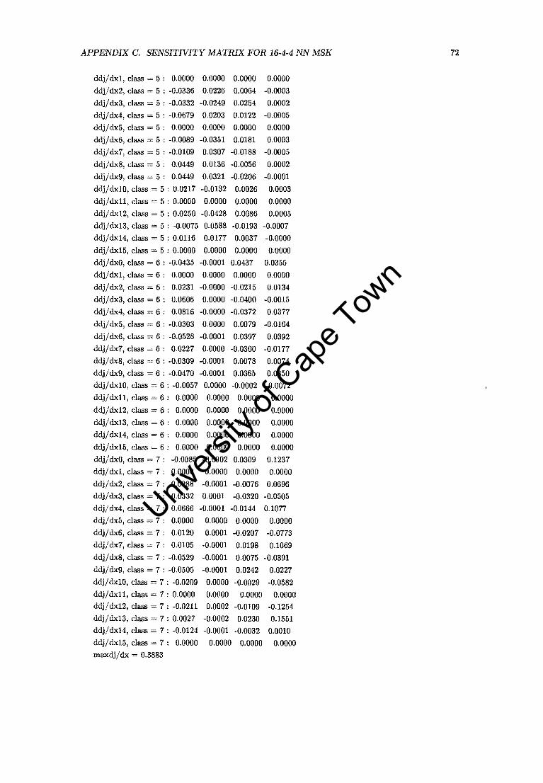
APPENDIX C. SENSITIVITY MATRIX FOR 16-4-4 NN MSK 72
ddj/dx1, class = 5 : 0.0000 0.0000 0.0000 0.0000
ddj/dx2, class 5: -0.0336 0.0226 0.0064 -0.0003
ddj/dx3, class 5 : -0.0332 -0.0249 0.0254 0.0002
ddj/dx4, class = 5 : -0.0679 0.0203 0.0122 -0.0005
ddj/dx5, class = 5 : 0.0000 0.0000 0.0000 0.0000
ddj/dx6, class = 5 : -0.0089 -0.0351 0.0181 0.0003
ddj/dx7, class = 5 : -0.0109 0.0307 -0.0188 -0.0005
ddj/ dx8, class 5: 0.0449 0.0136 -0.0056 0.0002
ddj/dx9, class 5: 0.0449 0.0321 -0.0206 -0.0001
ddj/dx10, class 5: 0.0217 -0.0132 0.0026 0.0003
ddj/dxll, class = 5 : 0.0000 0.0000 0.0000 0.0000
ddj/dx12, class = 5 : 0.0250 -0.0428 0.0086 0.0005
ddj/dx13, class = 5 : -0.0075 0.0588 -0.0193 -0.0007
ddj/dx14, class 5: 0.0116 0.0177 0.0037 -0.0000
ddj/dx15, class 5: 0.0000 0.0000 0.0000 0.0000
ddj/dxO, class 6: -0.0435 -0.0001 0.0437 0.0355
ddj/dx1, class = 6 : n.oooo 0.0000 0.0000 0.0000
ddj/ dx2, class = 6 : 0.0231 -0.0000 -0.0215 0.0134
ddj/dx3, class = 6 : 0.0606 0.0000 -0.0400 -0.0015
ddj/dx4, class 6: 0.0816 -0.0000 -0.0372 0.0377
ddj/dx5, class 6 : -0.0303 0.0000 0.0079 -0.0164
ddj/dx6, class 6 : -0.0528 -0.0001 0.0397 0.0392
ddj/dx7, class = 6 : 0.0227 0.0000 -0.0300 -0.0177
ddj/dx8, class = 6 : -0.0309 -0.0001 0.0078 0.0074
ddj/dx9, class = 6 : -0.0470 -0.0001 0.0365 0.0350
ddj/dx10, class 6 : -0.0057 0.0000 -0.0002 -0.0072
ddj/dxll, class 6 : 0.0000 0.0000 0.0000 0.0000
ddj/dx12, class 6: 0.0000 0.0000 0.0000 0.0000
ddj/dx13, class = 6 : 0.0000 0.0000 0.0000 0.0000 ddj/dx14, class = 6 : 0.0000 0.0000 0.0000 0.0000
ddj/dx15, class = 6 : 0.0000 0.0000 0.0000 0.0000
ddj/dxO, class 7: -0.0085 -0.0002 0.0309 0.1237
ddj/dx1, class 7 : 0.0000 0.0000 0.0000 0.0000
ddj/dx2, class = 7 : 0.0288 -0.0001 -0.0076 0.0696
ddj/dx3, class = 7 : 0.0332 0.0001 -0.0320 -0.0505
ddj/ dx4, class := 7 : 0.0666 -0.0001 -0.0144 0.1077
ddj/ dx5, class 7: 0.0000 0.0000 0.0000 0.0000 ddj/dx6, class 7: 0.0120 0.0001 -0.0207 -0.0773
ddj/dx7, class 7: 0.0105 -0.0001 0.0198 0.1069
ddj/dx8, class = 7 : -0.0529 -0.0001 0.0075 -0.0391
ddj/dx9, class = 7 : -0.0505 -0.0001 0.0242 0.0227
ddj/dxlO, class = 7 : -0.0209 0.0000 -0.0029 -0.0582
ddj/dxll, class = 7 : 0.0000 0.0000 0.0000 0.0000 ddj/dx12, class 7: -0.0211 0.0002 -0.0109 -0.1254
ddj/dx13, class 7: 0.0027 -0.0002 0.0230 0.1551 ddj/dx14, class 7: -0.0124 -0.0001 -0.0032 0.0010
ddj/dx15, class = 7 : 0.0000 0.0000 0.0000 0.0000
maxdj/dx 0.3883
Univers
ity of
Cap
e Tow
n
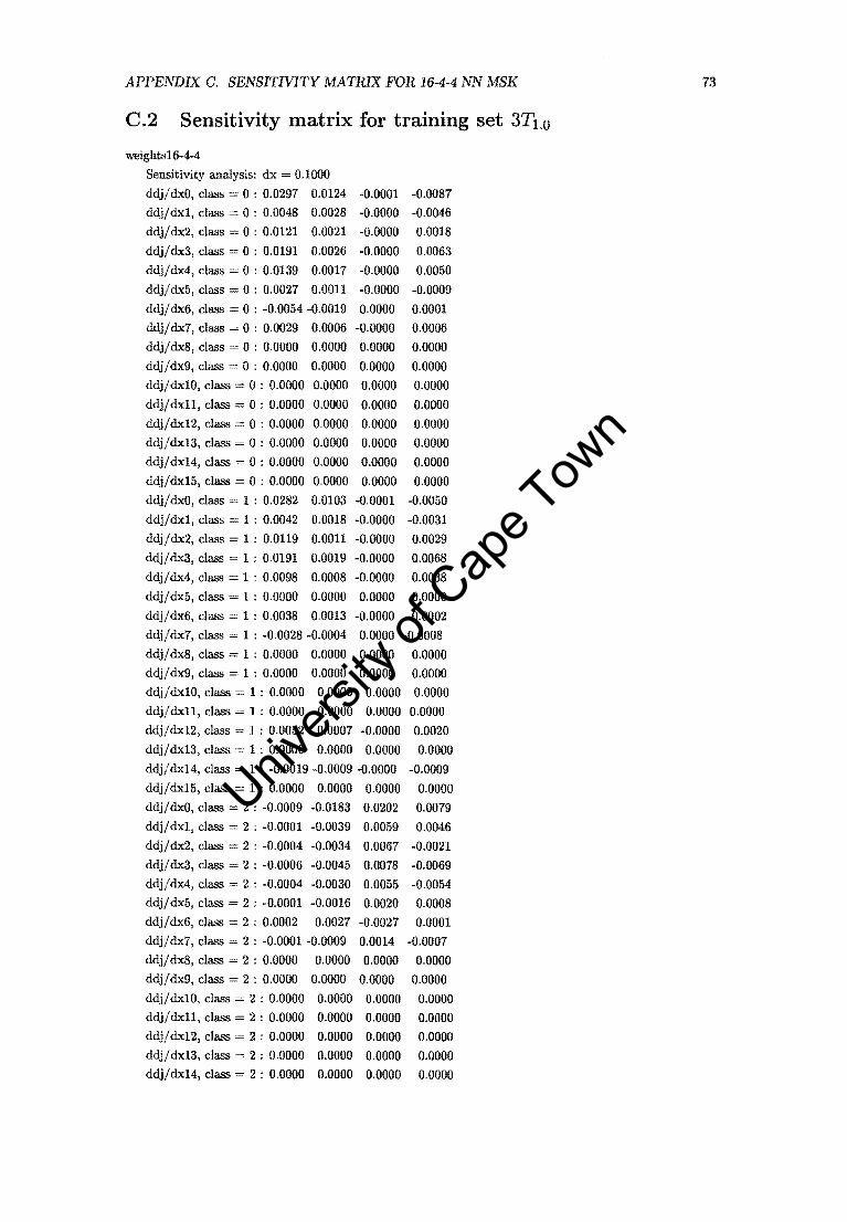
APPENDIX C. SENSITNITY MATRIX FOR 16-4-4 NN MSK 73
C.2 Sensitivity matrix for training set 3Tl.o
weights16-4-4
Sensitivity analysis: dx = 0.1000
ddj/dxO, class = 0 : 0.0297 0.0124 -0.0001 -0.0087
ddj/dx1, class = 0 : 0.0048 0.0028 -0.0000 -0.0046
ddj/dx2, class = 0 : 0.0121 0.0021 -0.0000 0.0018
ddj/dx3, class = 0 : 0.0191 0.0026 -0.0000 0.0063
ddjfdx4, class 0: 0.0139 0.0017 -0.0000 0.0050
ddj/dx5, class 0: 0.0027 0.0011 -0.0000 -0.0009
ddj/ dx6, class = 0 : -0.0054 -0.0019 0.0000 0.0001
ddj/dx7, class = 0 : 0.0029 0.0006 -0.0000 0.0006
ddj/dx8, class 0: 0.0000 0.0000 0.0000 0.0000
ddj/dx9, class 0: 0.0000 0.0000 0.0000 0.0000
ddj/dxlO, class 0: 0.0000 0.0000 0.0000 0.0000
ddj/dx11, class = 0 : 0.0000 0.0000 0.0000 0.0000
ddj/dx12, class = 0 : 0.0000 0.0000 0.0000 0.0000
ddj/dx13, class = 0 : 0.0000 0.0000 0.0000 0.0000
ddj/ dx14, class = 0 : 0.0000 0.0000 0.0000 0.0000
ddj/dx15, class = 0 : 0.0000 0.0000 0.0000 0.0000
ddj/ dxO, class 1 : 0.0282 0.0103 -0.0001 -0.0050
ddj/dx1, class 1: 0.0042 0.0018 -0.0000 -0.0031
ddj/dx2, class = 1 : 0.0119 0.0011 -0.0000 0.0029
ddj/dx3, class = 1 : 0.0191 0.0019 -0.0000 0.0068
ddj/dx4, class = 1 : 0.0098 0.0008 -0.0000 0.0038
ddj/ dx5, class 1: 0.0000 0.0000 0.0000 0.0000
ddj/dx6, class 1: 0.0038 0.0013 -0.0000 0.0002
ddj/dx7, class 1 : -0.0028 -0.0004 0.0000 -0.0008
ddj/ dx8, class = 1 : 0.0000 0.0000 0.0000 0.0000
ddj/dx9, class = 1 : 0.0000 0.0000 0.0000 0.0000
ddj/dxlO, class = 1 : 0.0000 0.0000 0.0000 0.0000
ddj/dx11, class = 1 : 0.0000 0.0000 0.0000 0.0000
ddj/dxI2, class 1 : 0.0052 0.0007 -0.0000 0.0020
ddj/dx13, class 1: 0.0000 0.0000 0.0000 0.0000
ddj/dx14, class = 1 : -0.0019 -0.0009 -0.0000 -0.0009
ddjfdxl5, class = 1 : 0.0000 0.0000 0.0000 0.0000
ddj/dxO, class = 2 : -0.0009 -0.0183 0.0202 0.0079
ddj/dx1, class 2 : -0.0001 -0.0039 0.0059 0.0046
ddj/dx2, class 2: -0.0004 -0.0034 0.0067 -0.0021
ddj/ dx3, class 2 : -0.0006 -0.0045 0.0078 -0.0069
ddj/dx4, class = 2 : -0.0004 -0.0030 0.0055 -0.0054
ddj/dx5, class = 2 : -0.0001 -0.0016 0.0020 0.0008
ddj/dx6, class = 2 : 0.0002 0.0027 -0.0027 0.0001
ddj/dx7, class 2 : -0.0001 -0.0009 0.0014 -0.0007
ddj/ dx8, class 2: 0.0000 0.0000 0.0000 0.0000
ddj/dx9, class = 2 : 0.0000 0.0000 0.0000 0.0000
ddj/dxlO, class = 2: 0.0000 0.0000 0.0000 0.0000
ddj/dx11, class = 2 : 0.0000 0.0000 0.0000 0.0000
ddj/dx12, class = 2 : 0.0000 0.0000 0.0000 0.0000
ddj/dxI3, class 2: 0.0000 0.0000 0.0000 0.0000 ddj/ dx14, class 2: 0.0000 0.0000 0.0000 0.0000
Univers
ity of
Cap
e Tow
n
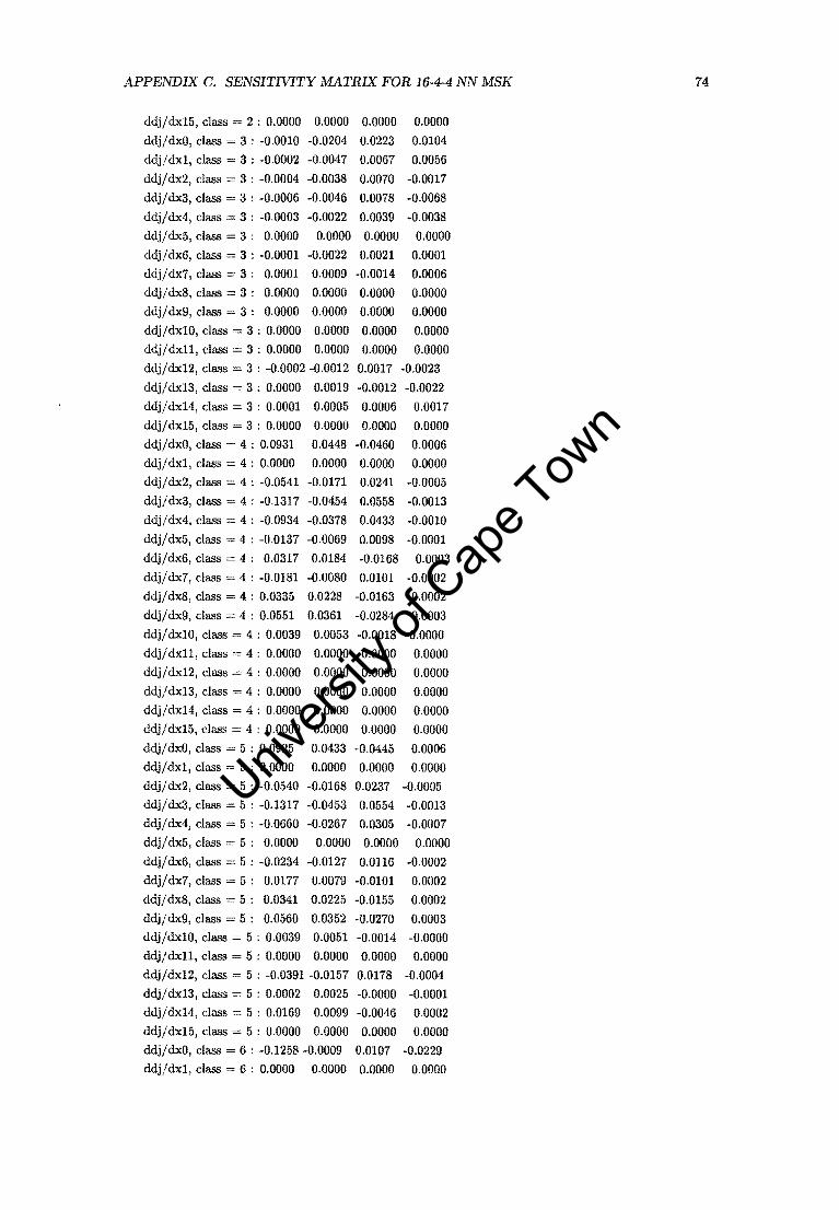
APPENDIX C. SENSITIVITY MATRIX FOR 16-4-4 NN MSK 74
ddj/dx15, class 2: 0.0000 0.0000 0.0000 0.0000
ddj/dxO, class 3 : -0.0010 -0.0204 0.0223 0.0104
ddj/dx1, class 3 : -0.0002 -0.0047 0.0067 0.0056
ddj/ dx2, class = 3 : -0.0004 -0.0038 0.0070 -0.0017
ddj/dx3, class = 3 : -0.0006 -0.0046 0.0078 -0.0068
ddj/dx4, class 3 : -0.0003 -0.0022 0.0039 -0.0038
ddj/dx5, class = 3 : 0.0000 0.0000 0.0000 0.0000
ddj/dx6, class = 3 : -0.0001 -0.0022 0.0021 0.0001
ddj/dx7, class 3: 0.0001 0.0009 -0.0014 0.0006
ddj/dx8, class:::: 3 : 0.0000 0.0000 0.0000 0.0000
ddj/dx9, class 3 : 0.0000 0.0000 0.0000 0.0000
ddj/dxlO, class 3: 0.0000 0.0000 0.0000 0.0000
ddj/dxll, class = 3 : 0.0000 0.0000 0.0000 0.0000
ddj/dx12, class 3 : -0.0002 -0.0012 0.0017 -0.0023
ddj/dx13, class 3: 0.0000 0.0019 -0.0012 -0.0022
ddj/dx14, class:::: 3 : 0.0001 0.0005 0.0006 0.0017
ddj/dx15, class 3: 0.0000 0.0000 0.0000 0.0000
ddj/dxO, class = 4 : 0.0931 0.0448 -0.0460 0.0006
ddj/dx1, class:::: 4 : 0.0000 0.0000 0.0000 0.0000
ddj/dx2, class 4 : -0.0541 -0.0171 0.0241 -0.0005
ddj/dx3, class = 4 : -0.1317 -0.0454 0.0558 -0.0013
ddj/dx4, class:::: 4 : -0.0934 -0.0378 0.0433 -0.0010
ddj/ dx5, class 4 : -0.0137 -0.0069 0.0098 -0.0001
ddj/dx6, class = 4 : 0.0317 0.0184 -0.0168 0.0003
ddj/dx7, class 4 : -0.0181 -0.0080 0.0101 -0.0002
ddj/dx8, class = 4 : 0.0335 0.0228 -0.0163 0.0002
ddj/dx9, class = 4 : 0.0551 0.0361 -0.0284 0.0003
ddj/ dx10, class = 4 : 0.0039 0.0053 -0.0018 -0.0000
ddj/dxll, class 4: 0.0000 0.0000 0.0000 0.0000
ddj/dx12, class = 4 : 0.0000 0.0000 0.0000 0.0000
ddj/dx13, class = 4 : 0.0000 0.0000 0.0000 0.0000 ddj/dx14, class = 4 : 0.0000 0.0000 0.0000 0.0000
ddj/dx15, class = 4 : 0.0000 0.0000 0.0000 0.0000
ddj/ dxO, class 5: 0.0925 0.0433 -0.0445 0.0006
ddj/dx1, class = 5 : 0.0000 0.0000 0.0000 0.0000
ddj/dx2, class :::: 5 : -0.0540 -0.0168 0.0237 -0.0005
ddj/dx3, class 5 : -0.1317 -0.0453 0.0554 -0.0013
ddj/dx4, class :::: 5 : -0.0660 -0.0267 0.0305 -0.0007
ddj/ dx5, class 5: 0.0000 0.0000 0.0000 0.0000
ddj/dx6, class 5: -0.0234 -0.0127 0.0116 -0.0002
ddj/dx7, class = 5 : 0.0177 0.0079 -0.0101 0.0002
ddj/dx8, class 5: 0.0341 0.0225 -0.0155 0.0002
ddj/dx9, class 5: 0.0560 0.0352 -0.0270 0.0003
ddj/dxlO, class = 5 : 0.0039 0.0051 -0.0014 -0.0000
ddj/dxll, class 5: 0.0000 0.0000 0.0000 0.0000
ddj/dx12, class 5 : -0.0391 -0.0157 0.0178 -0.0004
ddj/dx13, class = 5 : 0.0002 0.0025 -0.0000 -0.0001
ddj/dx14, class 5: 0.0169 0.0099 -0.0046 0.0002
ddj/dxI5, class 5: 0.0000 0.0000 0.0000 0.0000
ddj/dxO, class = 6 : -0.1258 -0.0009 0.0107 -0.0229
ddj/dx1, class 6: 0.0000 0.0000 0.0000 0.0000
Univers
ity of
Cap
e Tow
n

APPENDIX C. SENSITIVITY MATRIX FOR 16-4-4 NN MSK
ddj/dx2, class = 6 : 0.0638
ddj/dx3, class 6: 0.1663
ddj/dx4, class = 6 : 0.1411
0.0003 -0.0061
0.0009 -0.0133
0.0008 -0.0094
0.0198
0.0535
0.0412
ddj/dx5, class = 6 : 0.0240 0.0001 -0.0020 0.0036
ddj/dx6, class 6: -0.0565 -0.0004 0.0033 -0.0111
ddjfdx7, class = 6 : 0.0306 0.0002 -0.0021 0.0075
ddj/dx8, class = 6 : -0.0584 -0.0005 0.0033 -0.0087
ddj/dx9, class 6: -0.0910 -0.0007 0.0059 -0.0114
ddj/dxlO, class = 6 : -0.0060 -0.0001 0.0004 0.0023
ddj/dx11, class 6: 0.0000 0.0000 0.0000 0.0000
ddj/dx12, class 6: 0.0000 0.0000 0.0000 0.0000
ddj/dx13, class = 6 : 0.0000 0.0000 0.0000 0.0000
ddj/dx14, class = 6 : 0.0000 0.0000 0.0000 0.0000
ddj/dx15, class 6: 0.0000 0.0000 0.0000 0.0000
ddj/dxO, class = 7 : -0.1248 -0.0009 0.0104 -0.0246
ddj/dxl, class = 7: 0.0000 0.0000 0.0000 0.0000
ddj/dx2, class = 7 : 0.0636 0.0003 -0.0060 0.0200
ddj/dx3, class = 7 : 0.1661 0.0009 -0.0134 0.0531
ddj/dx4, class = 7 : 0.0997 0.0005 -0.0067 0.0288
ddj/dx5, class = 7 : 0.0000 0.0000 0.0000 0.0000
ddj/ dx6, class 7: 0.0392 0.0003 -0.0024 0.0083
ddj/dx7, class 7 : -0.0307 -0.0002 0.0020 -0.0075
ddjfdx8, class = 7 : -0.0576 -0.0005 0.0032 -0.0093
ddj/dx9, class 7 : -0.0895 -0.0007 0.0058 -0.0128
ddj/dxlO, class 7 : -0.0058 -0.0001 0.0003 0.0019
ddj/dxll, class = 7 : 0.0000 0.0000 0.0000 0.0000
ddj/ dx12, class = 7 : 0.0568 0.0003 -0.0039 0.0161
ddj/dx13, class 7 : -0.0003 -0.0001 0.0000 0.0025
ddj/ dx14, class = 7 : -0.0259 -0.0002 0.0010 -0.0070
ddj/dx15, class 7: 0.0000 0.0000 0.0000 0.0000
maxdj/dx 0.1663
75
Univers
ity of
Cap
e Tow
n

Appendix D
Simulations Software: Commsim
D.1 Functions
The following tables list all the functions used for performing the simulations.
Table D.l: Modulator functions f gen mcpfskO; Generate m-ary CPFSK signal oscO; Sinusoidal signal source mapper tilted4cpfskOi Mapper for tilted 4-ary CPFSK
Table D.2: Decoder functions I f v4cpfskO; Viterbi decoder for 4-ary CPFSK I f vrnskO; Viterbi decoder for MSK I f f4cpfskO; Fano decoder for 4-ary CPFSK
Table D.3: Demodulator functions fsk demodOi FSK demodulator fsk demodneuralOi FSK neural net demodulator
• cpfsk4 demodOi 4-ary CPFSK demodulator msk demod(); MSK demodulator msk demodneuralO; MSK neural net demodulator cpfsk4 demodneuralOi 4-ary CPFSK neural net demodulator
D.2 Function Instance Initialization and Data Storage
This section describes the method used to allocate private memory to each function instance. An
array of pointers to type double is declared in the main.c module (see section D.3 for information on the main.c module):
double *recind [MF - tJ ; 1* Declare an array of pointers to type double *1 1* MF = maximum number of functions *1
The address of one of these array elements is passed to the function. When a function is called
for the first time (at time = 0), it reserves a memory block of specific size for its personal use if
76
Univers
ity of
Cap
e Tow
n
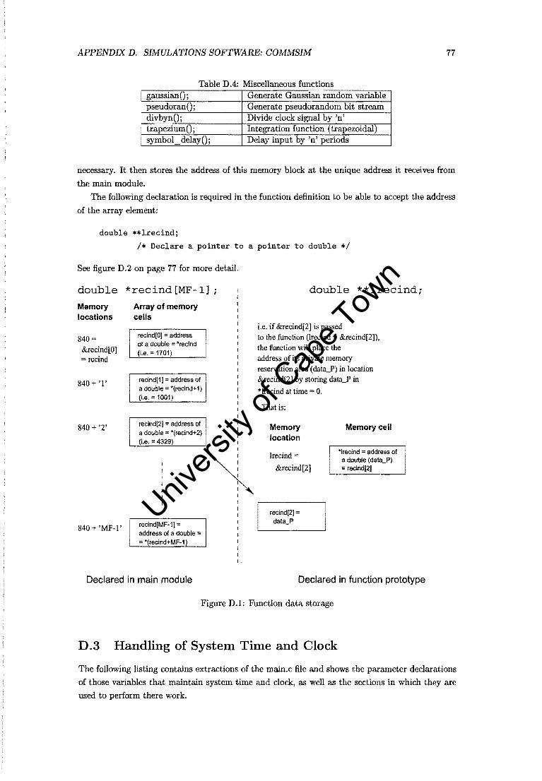
APPENDIX D. SIMULATIONS SOFTWARE: COMMSIM 77
Table D.4: Miscellaneous functions I gaussianO; Generate Gaussian random variable
pseudoranO; Generate pseudorandom bit stream divbynO; Divide clock signal by 'n' trapeziumO; Integration function (trapezoidal)
I symbol delayO; Delay input by 'n' periods
necessary. It then stores the address of this memory block at the unique address it receives from
the main module.
The following declaration is required in the function definition to be able to accept the address
of the array element:
double **lrecind;
1* Declare a pointer to a pointer to double *1
See figure D.2 on page 77 for more detaiL
double *recind[MF-l]
Memory locations
840= &recind[O] = recind
840 + '1'
840 + '2'
840 + 'MF-l'
Array of memory cells
recind[O) = address of a double:; *recind
(Le. = 1701)
recind[1] = address of a double *(recind+1) (i.e. = 1001)
recind[2] '" address of a double = *(recind+2) (Le. = 4329)
recind[MF-1J = address of a double :; :; '(recind+MF-1)
Declared in main module
~ I
I.
double **lrecind;
i.e. if &recind[2] is passed to the function (lrecind = &recind[2]), the function will place the address of its private memory reservation area (dataY) in location &recind[2] by storing data_P in
*Irecind at time = O.
That is:
Memory location
lrecind
&recind[2]
recind[2] = data_P
Memory cell
*Irecind = address of a double (data_P) = recind[2]
Declared in function prototype
Figure D.l: Function data storage
D.3 Handling of System Time and Clock
The following listing contains extractions of the main.c file and shows the parameter declarations
of those variables that maintain system time and clock, as well as the sections in which they are
used to perform there work.
Univers
ity of
Cap
e Tow
n

APPENDIX D. SIMULATIONS SOFTWARE: GOMMSIM
\* function main.c *\
unsigned long t, tmax;
unsigned char clk, prev_clk;
double time, tstep, clktdown, clktup, clkper;
78
1* t : counter used to increment system time with simulation timestep value *1 1* tmax : maximum number of time steps *1 1* clktdown, clktup : parameters that set the on/off ratio of the clock *1
void mainO {
extern unsigned long t, tmax;
extern unsigned char clk, prev_clk;
extern double time, tstep, clktdown, clktup, clkper;
tstep = Ts/20; 1* Setting simulation time step
time 0;
tmax 2000;
clk = 1;
clkper Ts;
clktdown = 0.5*clkper;
clktup = clkper;
prev_clk = (clk + 1) % 2;
for (t = 0; t <= tmax; t++) {
Symbol period I x *1
1****************************************************1 1* Do function processing at each multiple of tstep *1 1* User input: *1 1. Encoding functions(vout. vin, time, tstep, &recind[xx]);
2. Modulation functions ...
3. Add channel perturbations
4. Demodulation functions
5. Decoding functions ..•
6. Data collection and output
1****************************************************1 1* Update "time" and when required, the clock "clk" *1 prev_clk clk;
time time + tstep;
if (time >= (clktdown - 0.0000001» {
clk 0;
clktdown = clktdown + clkper; }
if (time >= (clktup - 0.0000001» {
clk = 1;
Univers
ity of
Cap
e Tow
n

APPENDIX D. SIMULATIONS SOFTWARE: COMMSIM
clktup = clktup + clkper; }
1* Generate new Pseudo-random bit:
Update shift registers of PRandom MLFSR,
see fig 8-20, p. 527 Z & p *1 etc. }
} 1* End of function "main" *1
79
Univers
ity of
Cap
e Tow
n

Bibliography
[1] J.B. Anderson, T. AuIin, and C.E. Sundberg. Digital Phase Modulation. Plenum Press, 1986.
[2] T. AuIin, and C.E. Sundberg. Continuous phase modulation - Part I: Full response signaling.
IEEE Transactions on Communications, COM-29(3):196-209, March 1981.
[3] T. AuIin, N. Rydbeck and C.E. Sundberg. Continuous phase modulation - Part IT: Partial
response signaling. IEEE Transactions on Communications, COM-29(3):21O-225, March 1981.
[4] J.B. Anderson, D.P. Taylor. A Bandwidth-efficient class of signal-space codes. IEEE Trans
actions on Information Theory. Vol-IT(30):703-712, November 1978.
[5] P. G. Anderson, RS. Gaborski, M. Ge, S. Raghavendra, M. Lung. Using Quasi-random
Numbers in Neural Networks. Research Paper, FTP: ftp.cs.rit.edu, Directory: \pub\pga,
File: quasi-NN.ps.
[6] J. Cuthbert. Multi-h demodulation. PhD thesis, University of Cape Town, 1998.
[7] R O. Duda and P. E. Hart. Pattern Classification and Scene Analysis. John Wiley & Sons,
New York (1973)
[8] M.V. Eyuboglu, S.U. Qureshi. Reduced-State Sequence Estimation with Set Partitioning and
Decision Feedback. IEEE Transactions on Communications, Vol-36(1):13-20, January 1988.
[9} RM. Fano. A Heuristic Discussion of Probabilistic Decoding. IEEE Transactions on Infor
mation Theory, Vol-9:64-74, April 1963.
[10] G.D. Forney, JR The Viterbi Algorithm. Proceedings of the IEEE, Vol-61(3):268-277, March
1973.
[1 :1.] M.S. Hodgart, B. Bohm, and J .A. Schoonees. A robust coherent receiver for MSK. Submitted
to IEEE Transactions on Communications, June 1996.
[12] J. Huber, W. Liu. An Alternative Approach to Reduced-Complexity CPM-Receivers. IEEE
Journal on Selected Areas in Communications, Vol-7(8):1437-1449, December 1989.
[13] S. Gish and W. Blanz. Comparing a connectionist trainable classifier with classical statistical
decision analysis methods. Res. Rep., IBM, Almaden Res. Cen., San Jose, CA, 1989.
[14] S.E. Kritzinger. An investigation into 4-CPFSK modulation and demodulation. MSc thesis,
University of Cape Town, 1994.
[15] R.P. Lippmann. An introduction to computing with neural nets. IEEE ASSP Magazine, Vol-4(2):4-22, April 1987.
80
Univers
ity of
Cap
e Tow
n

BIBLIOGRAPHY 81
[16] J.L. Massey. A generalized formulation of minimum shift keying. Conf. Rec. Int. Conf. Com
mun. ICC '80, volume 2, pages 26.5.1-26.5.4 IEEE, June 1980.
[17] J.L. Massey. The how and why of channel coding. Proceedings International Zurich Seminar,
pages 67-73, March 1984.
[18] Halvar B. Mathiesen. Neural Network Based Multi-h CPFSK Receivers. BSc thesis, University
of Cape Town, 1997.
[19] W.P. Osborne and M.B. Luntz. Coherent and noncoherent detection of CPFSK. IEEE Trans
actions on Communications, COM-22(8):1023-1026, August 1974.
[20] Theodore S. Rappaport. Wireless Communications. Prentice Hall PTR, 1996.
[21] B.E. Rimoldi. A Decomposition Approach to CPM. IEEE Transactions on Information The
ory, Vol-34(2):260-270, March 1988.
[22] B.E. Rimoldi. Continuous-Phase Modulation and Coding for Bandwidth and energy Efficiency.
PhD thesis, Swiss Federal Institute of Technology Zurich,1988.
[23] B.E. Rimoldi. Design of Coded CPFSK Modulation Systems for Bandwidth and Energy Effi
ciency. IEEE Tran,~actions on Communications, Vol-37(9):897-905, September 1989.
[24] B.E. Rimoldi. Exact Formula for the Minimum Squared Distance of CPFSK. IEEE Transac
tions on Communications, Vol-39(9):1280-1282, September 1991.
[25] R. Rosenblatt. Principles of Neurodynamics. New York, Spartan Books (1959).
[26] Thomas A. Schonhoff. Symbol Error Probabilities for M-ary CPFSK: Coherent and Non
coherent Detection. IEEE Transactions on Communications, COM-24:644-652, June 1976.
[27] J.A. Schoonees. A Likelihood Ratio Analysis of Continuous-Phase Frequency Shift Keying.
PhD thesis, University of Cape Town, 1998.
[28] Stuttgart. Stuttgart Neural Network Simulator (SNNS), User Manual Version 4.1. Institute for
Parallel and Distributed High Performance Systems (IPVR), University of Stuttgart. Report
No. 6/95.
[29] C-E. Sundberg. Continuous Phase Modulation. IEEE Communications Magazine, Vol-
24(4):25-38, April 1986.
[30] A. Svenson. Reduced State Sequence Detection of Full Response Continuous Phase Modula
tion. Electronic Letters, Vol-26(10):652-654, May 1990.
[31] Gabor C. Ternes and Jack W. LaPatra. Introduction to Circuit Synthesis and Design. McGraw
Hill Inc. 1977.
[32] G. de Veciana, A. Zakhor. Neural Net-Based Continuous Phase Modulation Receivers. IEEE
Transactions on Communications, Vol-40(8):1396-1408, August 1992.
[33] Xiao-an Wang and Stephen B. Wicker. An Artificial Neural Net Viterbi Decoder. IEEE Trans
actions on Communications, Vol-44(2):165-171, February 1996.
[34] John M. Wozencraft, Irwin M. Jacobs. Principles of Communication Engineering. Waveland
Press, Inc. 1965.
Univers
ity of
Cap
e Tow
n