quick-sort - ics.uci.edugoodrich/teach/cs260p/notes/quicksort.pdf · the worst case for quick-sort...

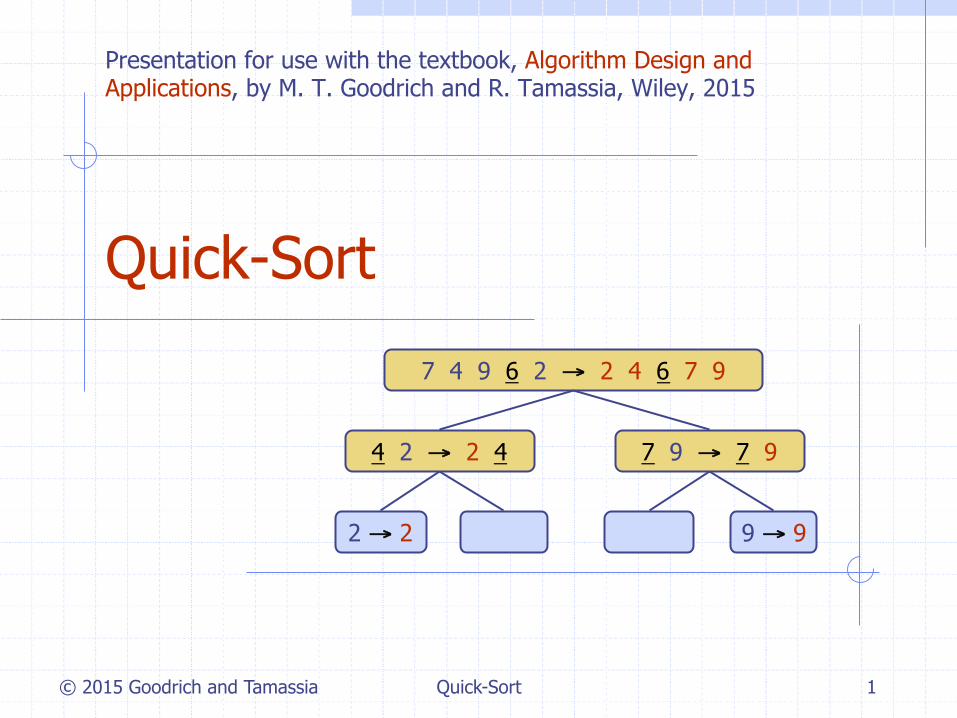
© 2015 Goodrich and Tamassia Quick-Sort 1

Quick-Sort

7 4 9 6 2 → 2 4 6 7 9

4 2 → 2 4 7 9 → 7 9

2 → 2 9 → 9

Presentation for use with the textbook, Algorithm Design and Applications, by M. T. Goodrich and R. Tamassia, Wiley, 2015


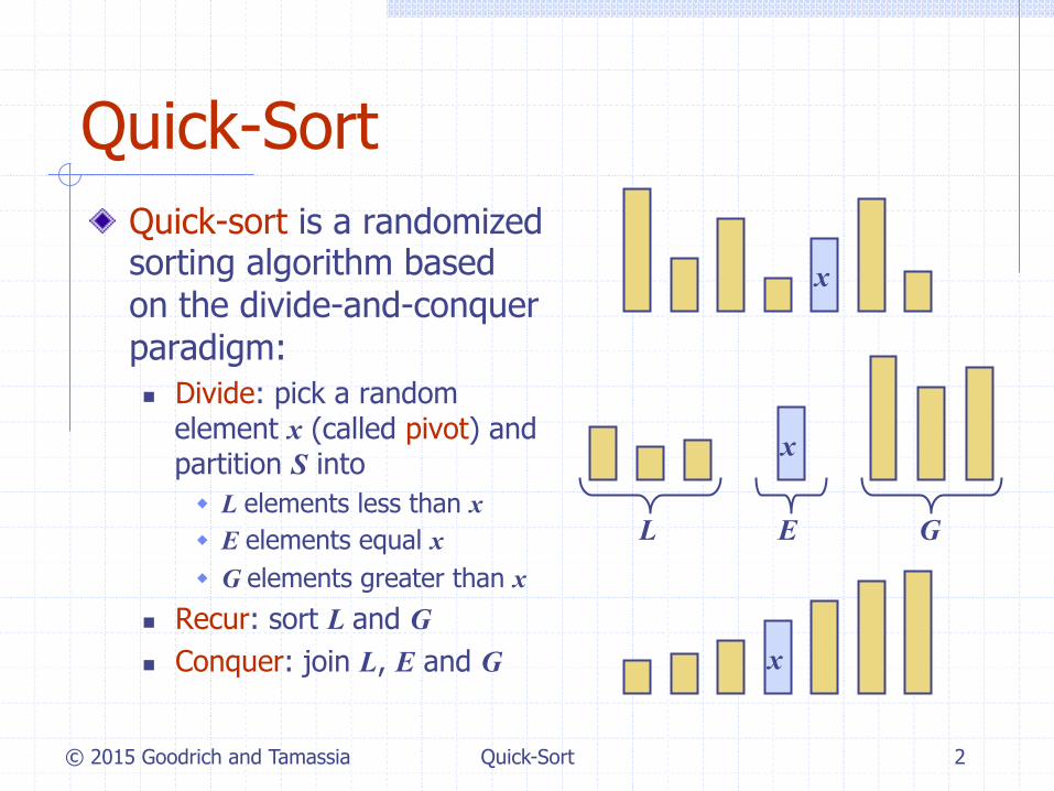
Quick-Sort Quick-sort is a randomized sorting algorithm based on the divide-and-conquer paradigm: n  Divide: pick a random

element x (called pivot) and partition S into w  L elements less than x w  E elements equal x w  G elements greater than x

n  Recur: sort L and G n  Conquer: join L, E and G

x

x

L G E

x


Partition We partition an input sequence as follows: n  We remove, in turn, each

element y from S and n  We insert y into L, E or G,

depending on the result of the comparison with the pivot x

Each insertion and removal is at the beginning or at the end of a sequence, and hence takes O(1) time Thus, the partition step of quick-sort takes O(n) time

Algorithm partition(S, p) Input sequence S, position p of pivot Output subsequences L, E, G of the elements of S less than, equal to, or greater than the pivot, resp. L, E, G ← empty sequences x ← S.remove(p) while ¬S.isEmpty()

y ← S.remove(S.first()) if y < x L.addLast(y) else if y = x E.addLast(y) else { y > x } G.addLast(y)

return L, E, G


Quick-Sort Tree An execution of quick-sort is depicted by a binary tree n  Each node represents a recursive call of quick-sort and stores

w  Unsorted sequence before the execution and its pivot w  Sorted sequence at the end of the execution

n  The root is the initial call n  The leaves are calls on subsequences of size 0 or 1

7 4 9 6 2 → 2 4 6 7 9

4 2 → 2 4 7 9 → 7 9

2 → 2 9 → 9


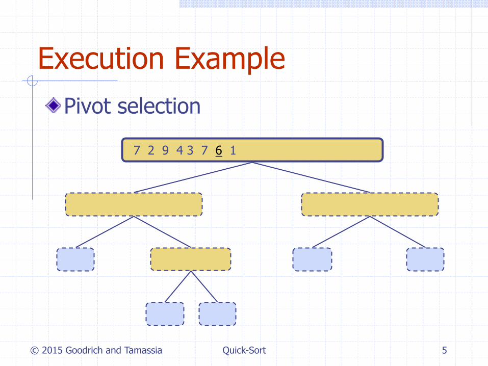
Execution Example Pivot selection

7 2 9 4 → 2 4 7 9

2 → 2

7 2 9 4 3 7 6 1 → 1 2 3 4 6 7 8 9

3 8 6 1 → 1 3 8 6

3 → 3 8 → 8 9 4 → 4 9

9 → 9 4 → 4


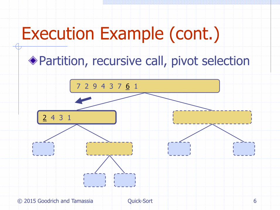
Execution Example (cont.) Partition, recursive call, pivot selection

2 4 3 1 → 2 4 7 9

9 4 → 4 9

9 → 9 4 → 4

7 2 9 4 3 7 6 1 → 1 2 3 4 6 7 8 9

3 8 6 1 → 1 3 8 6

3 → 3 8 → 8 2 → 2


Execution Example (cont.) Partition, recursive call, base case

2 4 3 1 →→ 2 4 7

1 → 1 9 4 → 4 9

9 → 9 4 → 4

7 2 9 4 3 7 6 1 → → 1 2 3 4 6 7 8 9

3 8 6 1 → 1 3 8 6

3 → 3 8 → 8


Execution Example (cont.) Recursive call, …, base case, join

3 8 6 1 → 1 3 8 6

3 → 3 8 → 8

7 2 9 4 3 7 6 1 → 1 2 3 4 6 7 8 9

2 4 3 1 → 1 2 3 4

1 → 1 4 3 → 3 4

9 → 9 4 → 4


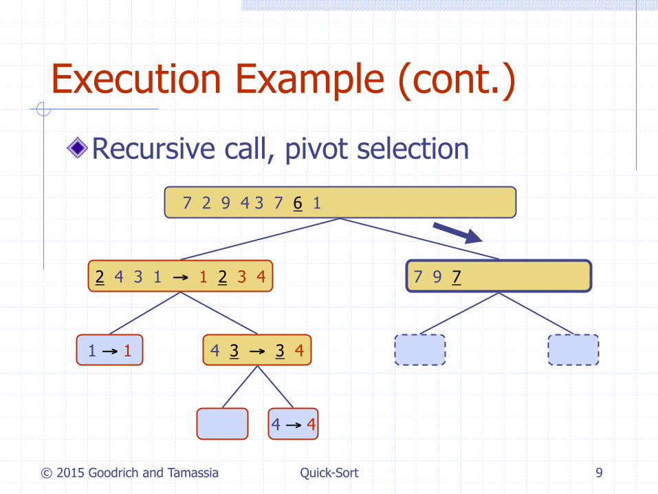
Execution Example (cont.)

Recursive call, pivot selection

7 9 7 1 → 1 3 8 6

8 → 8

7 2 9 4 3 7 6 1 → 1 2 3 4 6 7 8 9

2 4 3 1 → 1 2 3 4

1 → 1 4 3 → 3 4

9 → 9 4 → 4

9 → 9


Execution Example (cont.) Partition, …, recursive call, base case

7 9 7 1 → 1 3 8 6

8 → 8

7 2 9 4 3 7 6 1 → 1 2 3 4 6 7 8 9

2 4 3 1 → 1 2 3 4

1 → 1 4 3 → 3 4

9 → 9 4 → 4

9 → 9


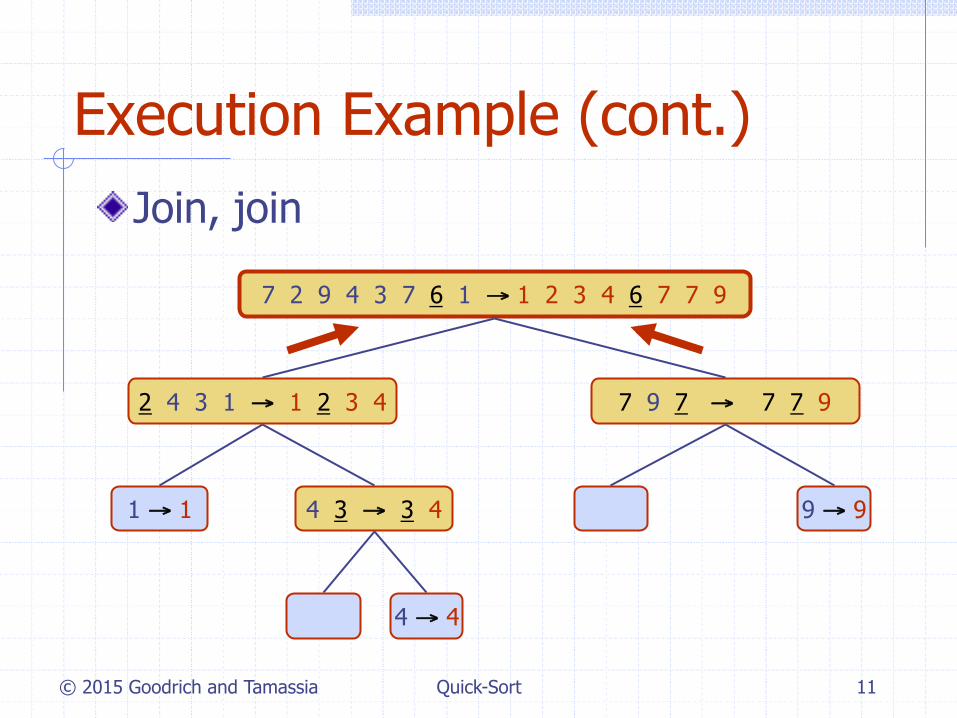
Execution Example (cont.) Join, join

7 9 7 → 17 7 9

8 → 8

7 2 9 4 3 7 6 1 → 1 2 3 4 6 7 7 9

2 4 3 1 → 1 2 3 4

1 → 1 4 3 → 3 4

9 → 9 4 → 4

9 → 9


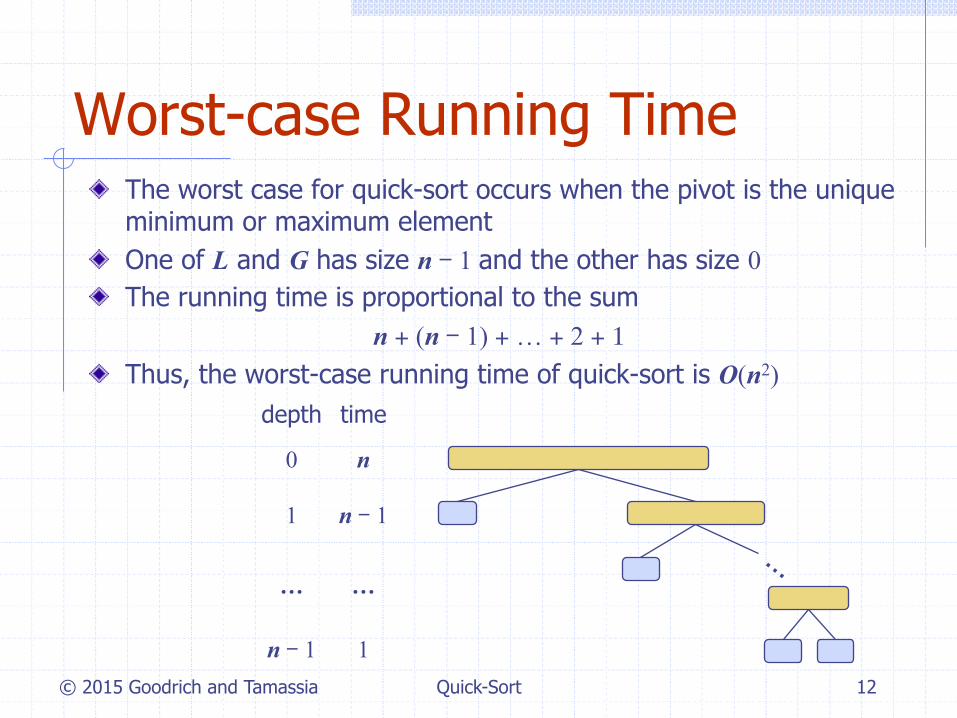
Worst-case Running Time The worst case for quick-sort occurs when the pivot is the unique minimum or maximum element One of L and G has size n - 1 and the other has size 0 The running time is proportional to the sum

n + (n - 1) + … + 2 + 1 Thus, the worst-case running time of quick-sort is O(n2)

depth time

0 n

1 n - 1

… …

n - 1 1


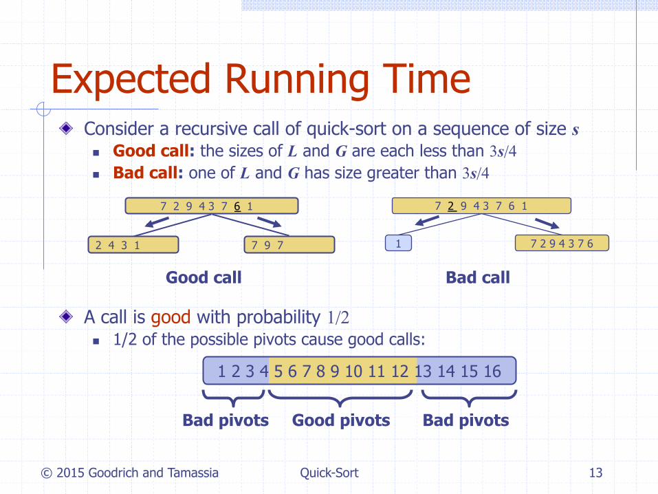
Expected Running Time Consider a recursive call of quick-sort on a sequence of size s n  Good call: the sizes of L and G are each less than 3s/4 n  Bad call: one of L and G has size greater than 3s/4

A call is good with probability 1/2 n  1/2 of the possible pivots cause good calls:

7 9 7 1 → 1

7 2 9 4 3 7 6 1 9

2 4 3 1 7 2 9 4 3 7 6 1

7 2 9 4 3 7 6 1

Good call Bad call

1 2 3 4 5 6 7 8 9 10 11 12 13 14 15 16

Good pivots Bad pivots Bad pivots


Expected Running Time, Part 2 Probabilistic Fact: The expected number of coin tosses required in order to get k heads is 2k For a node of depth i, we expect n  i/2 ancestors are good calls n  The size of the input sequence for the current call is at most (3/4)i/2n

s(r)

s(a) s(b)

s(c) s(d) s(f)s(e)

time per levelexpected height

O(log n)

O(n)

O(n)

O(n)

total expected time: O(n log n)

Therefore, we have n  For a node of depth 2log4/3n, the

expected input size is one n  The expected height of the

quick-sort tree is O(log n) The amount or work done at the nodes of the same depth is O(n) Thus, the expected running time of quick-sort is O(n log n)


In-Place Quick-Sort Quick-sort can be implemented to run in-place In the partition step, we use replace operations to rearrange the elements of the input sequence such that n  the elements less than the

pivot have rank less than h n  the elements equal to the pivot

have rank between h and k n  the elements greater than the

pivot have rank greater than k The recursive calls consider n  elements with rank less than h n  elements with rank greater

than k

Algorithm inPlaceQuickSort(S, l, r) Input sequence S, ranks l and r Output sequence S with the elements of rank between l and r rearranged in increasing order if l ≥ r

return i ← a random integer between l and r x ← S.elemAtRank(i) (h, k) ← inPlacePartition(x) inPlaceQuickSort(S, l, h - 1) inPlaceQuickSort(S, k + 1, r)


In-Place Partitioning Perform the partition using two indices to split S into L and E U G (a similar method can split E U G into E and G).

Repeat until j and k cross: n  Scan j to the right until finding an element > x. n  Scan k to the left until finding an element < x. n  Swap elements at indices j and k

3 2 5 1 0 7 3 5 9 2 7 9 8 9 7 6 9

j k

(pivot = 6)

3 2 5 1 0 7 3 5 9 2 7 9 8 9 7 6 9

j k


Summary of Sorting Algorithms Algorithm Time Notes

selection-sort O(n2) §  in-place §  slow (good for small inputs)

insertion-sort O(n2) §  in-place §  slow (good for small inputs)

quick-sort O(n log n) expected

§  in-place, randomized §  fastest (good for large inputs)

heap-sort O(n log n) §  in-place §  fast (good for large inputs)

merge-sort O(n log n) §  sequential data access §  fast (good for huge inputs)

quick-sort - ics.uci.edugoodrich/teach/cs260p/notes/quicksort.pdf · the worst case for quick-sort...

Documents