queuing system chap4 - ioe notes
TRANSCRIPT

Queuing SystemQueuing System
By Prof. S. Shakyay
1

Simulation of Queuing Systems
Introduction Waiting line queues are one of the most important areas, where
the technique of simulation has been extensively employed. The waiting lines or queues are a common site in real life The waiting lines or queues are a common site in real life. People at railway ticket window, vehicles at a petrol pump or at a
traffic signal, workers at a tool crib, products at a machining center television sets at a repair shop are a few examples ofcenter, television sets at a repair shop are a few examples of waiting lines.
2

Simulation of Queuing Systems
The waiting line situations arise, either because,The waiting line situations arise, either because,-There is too much demand on the service facility so
that the customers or entities have no wait for getting service, or
-There is too less demand, in which case the service f ilit h t it f th titifacility have to wait for the entities
The objective in the analysis of queuing situations is to balance the waiting time and idle time so as toto balance the waiting time and idle time, so as to keep the total cost at minimum.
3

Simulation of Queuing Systems
The queuing theory its development to anThe queuing theory its development to an engineer A.K.Earlang, who in 1920, studied waiting line queues of telephone calls in C h D kCopenhagen, Denmark.
The problem was that during the busy period, t l h t bl t h dltelephone operators were unable to handle the calls, there was too much waiting time, which resulted in customer dissatisfactionwhich resulted in customer dissatisfaction.
4

State Variables
customerqueueserver
State: InTheAir: number of aircraft either landing or
waiting to land
5
OnTheGround: number of landed aircraft RunwayFree: Boolean, true if runway available

Discrete Event Simulation Computationexample: air traffic at an airportexample: air traffic at an airportevents: aircraft arrival, landing, departure
arrival8:00 departure
9:15landedarrival9:30schedules
processed eventcurrent event
schedules
landed8:05
simulation time
unprocessed event
Events that have been scheduled, but have not been simulated (processed) yet are stored in a pending
6
simulated (processed) yet are stored in a pending event list
Events are processed in time stamp order; why?
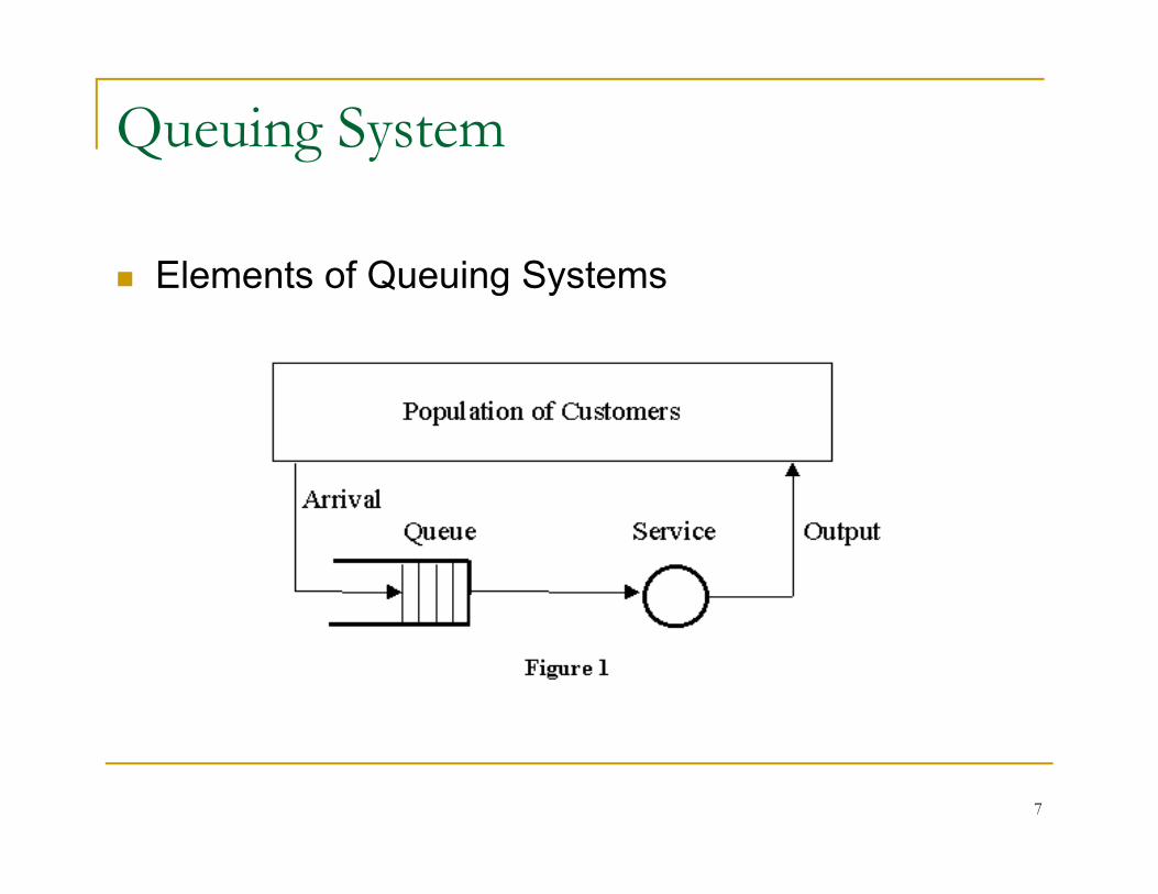
Queuing System
Elements of Queuing Systems Elements of Queuing Systems
7

Queuing System
Population of Customers or calling source can be considered either limited (closed systems) or unlimitedconsidered either limited (closed systems) or unlimited (open systems).
Unlimited population represents a theoretical model of systems with a large number of possible customers (asystems with a large number of possible customers (a bank on a busy street, a motorway petrol station).
Example of a limited population may be a number of processes to be run (served) by a computer or a certainprocesses to be run (served) by a computer or a certain number of machines to be repaired by a service man.
It is necessary to take the term "customer" very generally. Customers may be people machines of various nature Customers may be people, machines of various nature, computer processes, telephone calls, etc.
8

Queuing System
Arrival defines the way customers enter the Arrival defines the way customers enter the system.
Mostly the arrivals are random with random Mostly the arrivals are random with random intervals between two adjacent arrivals.
Typically the arrival is described by a random Typically the arrival is described by a random distribution of intervals also called Arrival PatternPattern.
9

Queuing System
Queue or waiting line represents a certain number of customers waiting for service (of course the queue may be empty).
Typically the customer being served is considered yp y gnot to be in the queue. Sometimes the customers form a queue literally (people waiting in a line for a bank teller). )
Sometimes the queue is an abstraction (planes waiting for a runway to land).
There are two important properties of a queue: There are two important properties of a queue: Maximum Size and Queuing Discipline.
10

Queuing System
Maximum Queue Size (also called SystemMaximum Queue Size (also called System capacity) is the maximum number of customers that may wait in the queue (plus the one(s) being
d)served). Queue is always limited, but some theoretical
models assume an unlimited queue lengthmodels assume an unlimited queue length. If the queue length is limited, some customers are
forced to renounce without being servedforced to renounce without being served
11

Applications of Queuing Theory
Telecommunications Traffic control Determining the sequence of computer
operations Predicting computer performance Health services (eg. control of hospital bed
assignments)Ai t t ffi i li ti k t l Airport traffic, airline ticket sales
Layout of manufacturing systems.
12

Example application of queuing theory
In many retail stores and banks In many retail stores and banks multiple line/multiple checkout system a
queuing system where customers wait for the next q g yavailable cashier
We can prove using queuing theory that : throughput improves increases when queues are used instead of separate lines
13

Example application of queuing theory
14

Queuing theory for studying networks
View network as collections of queuesView network as collections of queues FIFO data-structures
Queuing theory provides probabilistic g y p panalysis of these queues
Examples: Average length Average waiting time Probability queue is at a certain length Probability a packet will be lost
15

Model Queuing System
Queuing System
Queue Server
Server System Queuing System
Use Queuing models to Describe the behavior of queuing systems Evaluate system performance
16
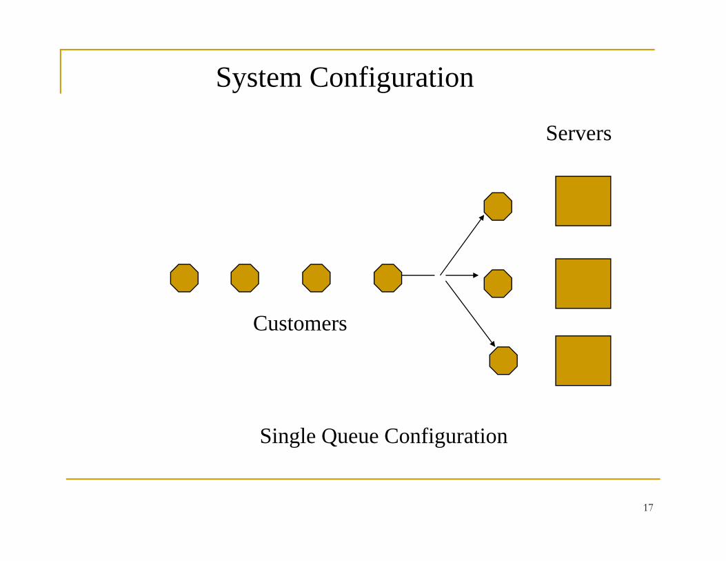
System Configuration
Servers
CCustomers
Single Queue Configuration
17

Characteristics of queuing systems
Arrival Process Arrival Process The distribution that determines how the tasks
arrives in the system.y Service Process The distribution that determines the task The distribution that determines the task
processing time Number of Servers Total number of servers available to process the
tasks
18

Queuing System
Queuing Discipline represents the way the queue is organized (r les of inserting and remo ing c stomers to/from the q e e)(rules of inserting and removing customers to/from the queue). There are these ways:
1) FIFO (First In First Out) also called FCFS (First Come First Serve) - orderly queue. ) y q
2) LIFO (Last In First Out) also called LCFS (Last Come First Serve) - stack.
3) SIRO (Serve In Random Order).4) Priority Queue, that may be viewed as a number of queues for
various priorities.5) Many other more complex queuing methods that typically change
the customer’s position in the queue according to the time spentthe customer s position in the queue according to the time spent already in the queue, expected service duration, and/or priority. These methods are typical for computer multi-access systems
19

Queuing System
Most quantitative parameters (like average queue q p ( g qlength, average time spent in the system) do not depend on the queuing discipline.
That’s why most models either do not take the That s why most models either do not take the queuing discipline into account at all or assume the normal FIFO queue.
In fact the only parameter that depends on the queuing discipline is the variance (or standard deviation) of the waiting time There is this importantdeviation) of the waiting time. There is this important rule (that may be used for example to verify results of a simulation experiment):
20

Queuing System
The two extreme values of the waiting time variance are for the FIFO q e e (minim m) and the LIFO q e e (ma im m)FIFO queue (minimum) and the LIFO queue (maximum).
Theoretical models (without priorities) assume only one queue. This is not considered as a limiting factor because practical
systems with more queues (bank with several tellers withsystems with more queues (bank with several tellers with separate queues) may be viewed as a system with one queue, because the customers always select the shortest queue.
Of course, it is assumed that the customers leave after being dserved.
Systems with more queues (and more servers) where the customers may be served more times are called Queuing Networks.Networks.
21

Queuing System Service represents some activity that takes time and
that the customers are waiting for. Again take it very generallygenerally.
It may be a real service carried on persons or machines, but it may be a CPU time slice, connection
d f l h ll b i h d fcreated for a telephone call, being shot down for an enemy plane, etc. Typically a service takes random time.
Theoretical models are based on random distribution of service duration also called Service Pattern.
Another important parameter is the number of Another important parameter is the number of servers. Systems with one server only are called Single Channel Systems, systems with more servers
ll d M lti Ch l S t22
are called Multi Channel Systems

Queuing System
Output represents the way customers leave the p p ysystem.
Output is mostly ignored by theoretical models, but sometimes the customers leaving the server entersometimes the customers leaving the server enter the queue again ("round robin" time-sharing systems).
Queuing Theory is a collection of mathematical models of various queuing systems that take as inputs parameters of the above elements and thatinputs parameters of the above elements and that provide quantitative parameters describing the system performance
23

Analysis of M/M/1 queue
Given: Given: • : Arrival rate of jobs (packets on input link) • : Service rate of the server (output link): Service rate of the server (output link)
Solve: L: average number in queuing system L: average number in queuing system Lq average number in the queue W: average waiting time in whole system W: average waiting time in whole system Wq average waiting time in the queue
24

M/M/1 queue model
LL
Lq
1
Wq
W
25

Kendall Notation 1/2/3(/4/5/6)
Six parameters in shorthand Six parameters in shorthand First three typically used, unless specified
1. Arrival Distribution2. Service Distribution3. Number of servers 4. Total Capacity (infinite if not specified) 5. Population Size (infinite) 6. Service Discipline (FCFS/FIFO)
26

Kendall Classification of Queuing Systems
The Kendall classification of queuing systems (1953) exists in several The Kendall classification of queuing systems (1953) exists in several modifications.
The most comprehensive classification uses 6 symbols: A/B/s/q/c/p
where:where: A is the arrival pattern (distribution of intervals between arrivals). B is the service pattern (distribution of service duration). s is the number of servers.
i th i di i li (FIFO LIFO ) O itt d f FIFO if t q is the queuing discipline (FIFO, LIFO, ...). Omitted for FIFO or if not specified.
c is the system capacity. Omitted for unlimited queues. p is the population size (number of possible customers). Omitted for open
systemssystems.
27

Kendall Classification of Queuing Systems
These symbols are used for arrival and service patterns: M is the Poisson (Markovian) process with exponential
distribution of intervals or service duration respectively. Em is the Erlang distribution of intervals or service
duration. D is the symbol for deterministic (known) arrivals and
constant service duration. G is a general (any) distribution. GI is a general (any) distribution with independent random g ( y) p
values.
28

Kendall Classification of Queuing Systems
Examples: D/M/1 = Deterministic (known) input, one
exponential server, one unlimited FIFO or unspecified queue, unlimited customer population.p q , p p
M/G/3/20 = Poisson input, three servers with any distribution, maximum number of customers 20, unlimited customer population.unlimited customer population.
D/M/1/LIFO/10/50 = Deterministic arrivals, one exponential server, queue is a stack of the maximum size 9 total number of customers 50maximum size 9, total number of customers 50.
29
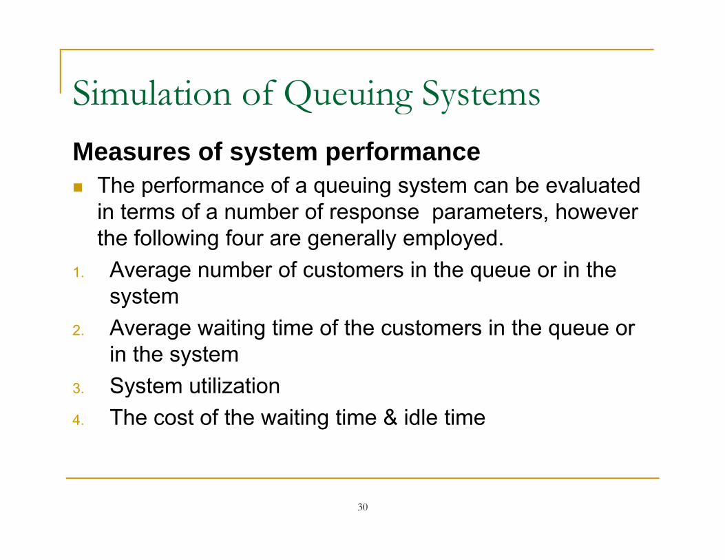
Simulation of Queuing SystemsSimulation of Queuing SystemsMeasures of system performance The performance of a queuing system can be evaluated
in terms of a number of response parameters, however the following four are generally employed.the following four are generally employed.
1. Average number of customers in the queue or in the system
2. Average waiting time of the customers in the queue or in the system
3 System utilization3. System utilization4. The cost of the waiting time & idle time
30

Simulation of Queuing SystemsMeasures of system performance
The knowledge of average number of customers in the queue or in the system helps to determine the
i t f th iti titi Al tspace requirements of the waiting entities. Also too long a waiting line may discourage the prospectus customers, while no queue may suggest that servicecustomers, while no queue may suggest that service offered is not of good quality to attract customers.
The knowledge of average waiting time in the queue is necessary for determining the cost of waiting in the queue.
31

Simulation of Queuing Systems
System Utilizationy System Utilization that is the percentage capacity utilized
reflects that extent to which the facility is busy rather than idle.
System utilization factor (s) is the ratio of average arrival rate (λ) to the average service rate (µ).
S= λ/µ in the case of a single server modelµ gS= λ/µn in the case of a “n” server model
The system utilization can be increased by increasing the arrival rate which amounts to increasing the averagethe arrival rate which amounts to increasing the average queue length as well as the average waiting time, as shown in fig 1. Under the normal circumstances 100% system utilization is not a realistic goal.
32

System Utilization
33Fig 1
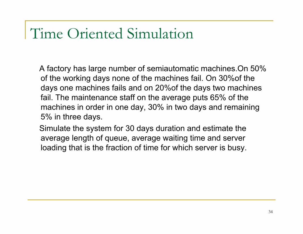
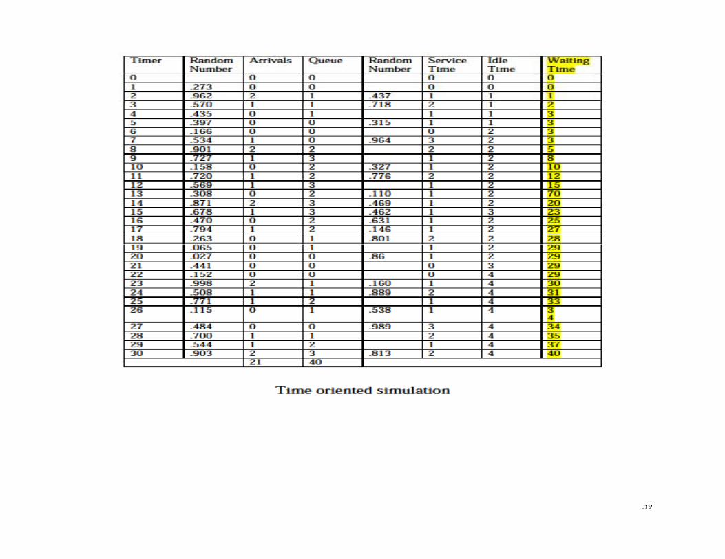
Time Oriented Simulation
A factory has large number of semiautomatic machines.On 50% y gof the working days none of the machines fail. On 30%of the days one machines fails and on 20%of the days two machines fail. The maintenance staff on the average puts 65% of the machines in order in one day, 30% in two days and remaining 5% in three days.Simulate the system for 30 days duration and estimate the y yaverage length of queue, average waiting time and server loading that is the fraction of time for which server is busy.
34

Time Oriented Simulation
Solution: Th i t i i l i d l Th f il f thThe given system is a single server queuing model. The failure of the
machines in the factory generates arrivals, while the maintenance staff is the service facility. There is no limit on the capacity of the system in other words on the length of waiting line. The population of machines is very large and can be taken as infinite.
Arrival pattern: On 50%of the days arrival=0O % fOn 30%of the days arrival=1On 20%of the days arrival=2Expected arrival rate=0*.5+1*.3+2*.2=0.7 per day.S i ttService pattern:65% machines in 1 day30% machines in 2 days5% machines in 3 da s
35
5% machines in 3 days

Time Oriented Simulation
Average service time: 1*.65+2*.3+3*.05=1.4 daysE t d i t 1/1 4 0 714 hi dExpected service rate=1/1.4=0.714 machines per dayThe expected arrival rate is slightly less than the expected service rate
and hence the system can reach a steady state. For the purpose of generating the arrivals per day and the services completed per g g p y p pday the given discrete distributions will be used.
Random numbers between 0 and 1 will be used to generate the arrivals as under.
0.0<r<=0.5 Arrivals=00.5<r<=0.8 Arrivals=10.8<r<=1.0Arrivals=2Si il l d b b t 0 d 1 ill b d fSimilarly, random numbers between 0 and 1 will be used for
generating the service times ( ST)0.0<r<=0.65ST=1day0 65<r<=0 95ST=2days
36
0.65<r<=0.95ST=2days0.95<r<=1.0 ST=3 days
Time Oriented Simulation In the time-oriented simulation, the timer is advanced in fixed steps
of time and at each step the system is scanned and updated. The time is kept very small, so that not many events occur during
this timethis time. All the events occurring during this small time interval are assumed
to occur at the end of the interval. At start of the simulation, the system that is the maintenance facility y y
can assumed to be empty, with no machine waiting for repair. On day 1, there is no machine in the repair facility. On day 2 there are 2 arrivals, the queue is made 2. Since service facility is idle, one arrival is put on service and queue
becomes 1. Server idle time becomes 1 day and the waiting time of customers
is also 1 day Timer is advanced by one dayis also 1 day. Timer is advanced by one day. The service time, ST is decreased by one and when ST becomes
zero facility becomes idle. Arrivals are generated which come out to be 1, it is added to the
37
g ,queue.
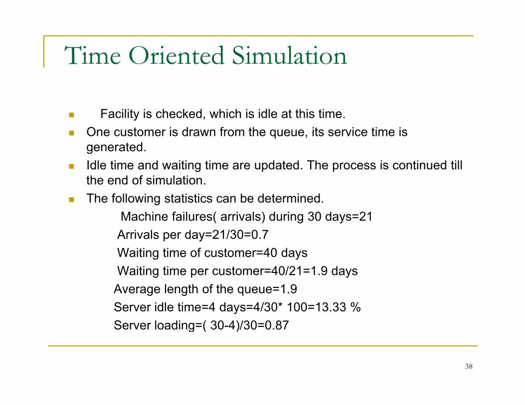
Time Oriented Simulation
Facility is checked, which is idle at this time. One customer is drawn from the queue, its service time is
generated. Idle time and waiting time are updated. The process is continued till
th d f i l tithe end of simulation. The following statistics can be determined.
Machine failures( arrivals) during 30 days=21Arrivals per day=21/30=0.7Waiting time of customer=40 daysWaiting time per customer=40/21=1.9 daysAverage length of the queue=1.9Server idle time=4 days=4/30* 100=13.33 %Server loading=( 30-4)/30=0.87
38
g ( )
39

Simulation on queuing systemTutorial
In a manufacturing system parts are being made at ag y p grate of one every 6 minutes. They are two types A andB and are mixed randomly with about 10 percent oftype B A separate inspector is assigned to examinetype B. A separate inspector is assigned to examineeach type of parts. The inspection of a part takes amean time of 4 minutes with a standard deviation of 2
i b B k i 20 i dminutes , but part B takes a mean time 20 minutes anda standard deviation of 10 minutes. Both inspectorsreject about 10% of the parts they inspect. Simulatej p y pthe system for total of 50 type A parts accepted anddetermine , idle time of inspectors and average time apart spends in system
40
part spends in system.