HAL Id: hal-03443584https://hal.archives-ouvertes.fr/hal-03443584

Submitted on 23 Nov 2021

HAL is a multi-disciplinary open accessarchive for the deposit and dissemination of sci-entific research documents, whether they are pub-lished or not. The documents may come fromteaching and research institutions in France orabroad, or from public or private research centers.

L’archive ouverte pluridisciplinaire HAL, estdestinée au dépôt et à la diffusion de documentsscientifiques de niveau recherche, publiés ou non,émanant des établissements d’enseignement et derecherche français ou étrangers, des laboratoirespublics ou privés.

Quaternary landscape dynamics boosted speciesdispersal across Southeast Asia

Tristan Salles, Claire Mallard, Laurent Husson, Sabin Zahirovic, Anta-ClarisseSarr, Pierre Sepulchre

To cite this version:Tristan Salles, Claire Mallard, Laurent Husson, Sabin Zahirovic, Anta-Clarisse Sarr, et al.. Quater-nary landscape dynamics boosted species dispersal across Southeast Asia. Communications Earth &Environment, Springer Nature, 2021, 2 (1), �10.1038/s43247-021-00311-7�. �hal-03443584�

ARTICLE

Quaternary landscape dynamics boosted speciesdispersal across Southeast AsiaTristan Salles 1✉, Claire Mallard1, Laurent Husson2, Sabin Zahirovic 1, Anta-Clarisse Sarr 3 &

Pierre Sepulchre 4

Sundaland, the inundated shelf separating Java, Sumatra and Borneo from the Malay

Peninsula, is of exceptional interest to biogeographers for its species richness and its position

at the junction between the Australasian and Indomalay biogeographic provinces. Owing to

its low elevation and relief, its physiography is contingent on relative sea-level change, which

drove Quaternary species burst in response to flooding episodes. New findings show that the

region was predominantly terrestrial during the Late Pleistocene requiring a reassessment of

the drivers of its recent biodiversity history. Here we show that physiographic changes have

modified the regional connectivity network and remodelled the pathways of species dispersal.

From combined landscape evolution and connectivity models, we found four phases of

drainage reorganisation and river captures. These changes have fragmented the environment

into multiple habitats connected by migratory corridors that cover 8% of the exposed shelf

and stretch across the biogeographic provinces. Our results support the theory that rapidly

evolving physiography could foster Quaternary biodiversification across Southeast Asia.

https://doi.org/10.1038/s43247-021-00311-7 OPEN

1 School of Geosciences, University of Sydney, Sydney, Australia. 2 CNRS, ISTerre, Université Grenoble-Alpes, Grenoble, France. 3 CL-Climat, CEREGE, Aix-en-Provence, France. 4 LSCE/IPSL, CEA-CNRS-UVSQ, Université Paris Saclay, Paris, France. ✉email: tristan.salles@sydney.edu.au

COMMUNICATIONS EARTH & ENVIRONMENT | (2021) 2:240 | https://doi.org/10.1038/s43247-021-00311-7 | www.nature.com/commsenv 1

1234

5678

90():,;

Based on the purported Quaternary geodynamic stability ofthe Sunda Shelf1–5, eustatic sea level fluctuations havegenerally been regarded as an important contributor to the

recent Southeast Asia extraordinary biological diversification6–9.Divergence and speciation would increase during eustatic high-stands and geographic dispersal during glacial sea level lowstands;this alternation would overall remodel the taxonomic composi-tion of the regional biotas3,10–13. Under these circumstances, sealevel oscillations would have acted as a species pump to increasethe regional terrestrial biodiversity1,10,14–16. New findings17,18

have challenged the idea of the prevalence of eustatic controls andhave demonstrated that the Sunda Shelf was subsiding through-out the Quaternary, being permanently subaerial before 400 ka.With Sundaland exposed for such a long period, the assumptionof sea level dominance is called into question implying that thedistribution of Sundaland biogeography either predates theQuaternary10,19,20 or is modulated by additional factors includingvariations of edaphic properties12,14,21, fragmentation of forestedhabitats4,8,21–23 or changes in paleoclimate conditions4,24,25.

In this study, we evaluate the contributions of overlookedsurface processes on the last 500 kyr biodiversity dynamic of theregion. Although investigations on the role that landscapes mighthave played in the biological evolution of Southeast Asia can betraced back to Darwin and Wallace1, limited work has beenconducted on the potential roles of geomorphology in shaping therelationships observed in the present-day assembly of the region’sbiota5,13,26,27.

Previous work28–30 has shown that changing landscapemorphology is a major driver of species dispersal strategies asthey track their optimum habitat31,32. Species running out ofsuitable habitats either become isolated, go extinct or are forcedto coexist with others and adapt. Fragmentation of habitatscould favour local endemism and higher speciation rates, bothof which contribute positively to increase biodiversity28,33. Herewe test the role of landscape dynamic in modifying connectivityand dispersal corridors across the exposed Sunda Shelf using aseries of calibrated surface evolution simulations34 forced witheustatic, climatic and tectonic conditions. From changing phy-siographic characteristics, we then estimate the spatio-temporalpermeability of the shelf to lowland evergreen rainforests speciesmovement using a connectivity model35. Finally, we use acombination of statistical approaches to quantify preferentialand persistent paleo-migration pathways across the shelf sincethe Late Pleistocene.

ResultsSensitivity of Sundaland flooding history to tectonic and sealevel conditions. To evaluate paleo-stream paths and associatedpaleo-drainage basins evolution, we performed a series of land-scape evolution simulations34 over the last one million years(Fig. 1a). Each simulation accounts for fluvial incision, sedimenttransport and deposition (in endorheic basins and in the marinerealm) as well as hillslope processes (Methods, Fig. 1b). All sce-narios are constrained by three external forcing mechanisms: (1)climate, as rainfalls, (2) eustatic sea level fluctuations, and (3)vertical tectonics. In this study, we tested five combinations ofthese forcing conditions (Supplementary Table 2). Two sea levelcurves were assessed (Supplementary Fig. 1c), the first threescenarios used the reconstruction from36 and the last two the sealevel stack proposed by37. We explored three different tectonicregimes. In scenario 1, we assumed no vertical deformation; in 2,a uniform subsidence rate of −0.25 mm/yr17, and for the last 3 weimposed a tectonic map (i.e., vertical land motion, SupplementaryFig. 1b) built from available regional uplift and subsidence rates(Methods, Supplementary Table 1). Finally, in all cases except

scenario 4 (where we assumed a uniform rainfall of 2 m/yr), weimposed derived precipitation estimates from the PaleoClimdatabase38–40. Landscape evolution models were calibratedagainst paleo-rivers derived from phylogenetic studies9,13 andseismic surveys as well as flooding events retrieved from bore-holes data41 in the Malay Basin (box A in Fig. 1b) and sedimentaccumulation across the Sunda Shelf41–44 (Methods, Supple-mentary Table 3). In summary, scenarios 1 and 2 are used toisolate the effects of tectonics, while scenario 4 is used as a controlfor rainfall regime. Scenarios 3 and 5 are used to evaluate the roleof sea level on the flooding history of the shelf.

We analysed the flooding history of Sundaland for the fiveproposed scenarios (Methods - Supplementary Fig. 1c) and foundthat except for the case with no subsidence (scenario 1), the shelfwas fully exposed prior to 400 ka (MIS 11) in agreement withprevious work17,18. At low sea level periods, sediments bypassthe shelf and accumulate in more distal offshore regions43

(Fig. 1b), while minimal shelf erosion is driven by river incision.Conversely, during marine transgressions, terrestrial sedimentsfluxes mostly rest on the shelf (Supplementary Fig. 1d). Over1Myr, our simulations predict up to 105 m of deposition(for scenario 1, Supplementary Table 3) in the Gulf of Thailandand around 300 m sediment accumulation on the continentalslope facing the southeast South China Sea (scenarios 2, 3 and 5 -Fig. 1b).

After 400 ka, level of marine incursions across the shelf arevariable between tested scenarios (Fig. 1c and SupplementaryFig. 1c), with incomplete (<80% of the shelf flooded) floodingevents during sea level highstands. For variable tectonicsubsidence and even when considering the sea level curve withthe highest amplitudes37 (scenario 5), pervasive (more than halfthe surface of the shelf) flooding prevails for <20% of the time(corresponding to ~80 kyr since MIS 11, Fig. 1c).

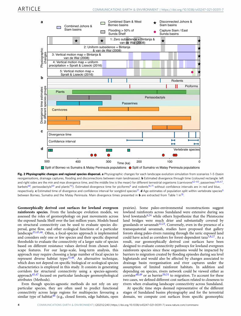
We found a clear sensitivity of the flooding history to bothtectonic and seal evel conditions. For all scenarios with imposedtectonic forcing (2–5), land bridges between Borneo andsurrounding regions are disrupted on several occasions.Conversely, most of the shelf remains subaerial over the lastmillion years, and the terrestrial connection from mainlandAsia to Java persists up to the Holocene. Our simulations refinerecent work on Sundaland subsidence17 and provide, for thefirst time, quantitative estimates of the timing and extent of theflooding episodes across the shelf (shaded grey areas in Fig. 2a).From Fig. 2b–d, compiled timing of the divergences fordifferent species groups and between populations varied widelyover the last 500 kyr and cannot be attributed to a single eventor mechanism such as eustatic sea level fluctuations18. Instead,this suggests that the divergences that did happen during theLate Pleistocene were more likely caused by a combination ofdifferent drivers acting on species diversification over tens ofthousands of years6. In the following sections, we investigatethe role that physiographic and climatic changes might haveplayed on this regional biological diversification and how itaffected Late Pleistocene diversification and post-divergenceflow from older speciation events.

Drainage basin reorganisation and river capture. Althoughpaleo-drainage systems have been invoked to explain the spatialdistribution of Southeast Asia freshwater aquatic species5,9,13,quantifying how physiographic changes might have affectedregional biota has never been done. Here our first step is tomodel the region’s geomorphological evolution by character-ising the main catchments dissecting the shelf and detailing inspace and time the major phases of drainage basin reorgani-sations (Fig. 3).

ARTICLE COMMUNICATIONS EARTH & ENVIRONMENT | https://doi.org/10.1038/s43247-021-00311-7

2 COMMUNICATIONS EARTH & ENVIRONMENT | (2021) 2:240 | https://doi.org/10.1038/s43247-021-00311-7 | www.nature.com/commsenv

In all models accounting for subsidence (scenarios 2–5),we found that successive marine regressions and transgressionspromote expansions and contractions of individual drainagebasins. This is indicated by the robust statistical correlationsbetween sea level fluctuations and catchments characteristics(Pearson’s coefficients in Fig. 3b and Supplementary Fig. 2). Wealso found a 30–50% decrease in drainage area for both the Siamand Johore rivers during the largest intermittent floodingepisodes (Fig. 3b and Supplementary Fig. 2).

In our simulations, the Mekong and Singapore main drainagedivides remain stable over time (Fig. 3a). When tectonic forcing isconsidered, the shelf experiences at least one phase of drainagebasin capture of the Johore and Siam catchments (shaded blueareas in Figs. 2a and 3b, Supplementary Figs. 2 and 3). For themodel presented in Fig. 3 (scenario 5), the Johore, Siam and WestBorneo rivers undergo several phases of drainage reorganisations.First, at around 330 ka, the Johore River captures neighbouringheadwaters from the Siam Basin. Following a phase of floodingaround 240 ka, the newly formed large drainage basin splits intotwo distinct catchments which have similar characteristics as theones before the capture (Fig. 3b). Since 200 ka, the Siam and WestBorneo basins also experienced two captures lasting for 60 and15 kyr, respectively. Finally, we notice a large capture of parts of

the Siam headwaters by the East Sunda Basin over the last 30 kyr.This capture lasts until the complete flooding of the Sunda Shelf10 kyr ago. The simulation from scenario 5, which includestectonics, sea level and precipitation maps constrained with Earthdata, reproduces the number of interpreted marine intrusions41

(Supplementary Table 2). In addition, the simulated cumulativedeposit thicknesses from this scenario is in the range of the onesobserved across the shelf (Supplementary Table 2). Finally, it alsoshows the maximum number of reorganisations between themain catchments, making it the best candidate to estimategeomorphological impacts on species migration (Fig. 2a).

These robust simulated geomorphic changes could be criticalto some species. For example, lowland freshwater biotas6,9,13,26

(Supplementary Fig. 1a and Table 4) have the ability to migrateacross the shelf from mainland Southeast Asia to both the MalayPeninsula, Sumatra, Borneo and Java based on simulated drainagebasins evolution and river captures (Fig. 3a and SupplementaryFig. 2). By comparing the major physiographic changes from oursimulations with divergence times from different groups ofterrestrial organisms over the past 320 kyr (Fig. 2b–d), we foundthat many of the Johore, Siam and West Borneo reorganisationsoften predate measured divergence times and population splitsfor the considered time period.

Fig. 1 Simulated landscape evolution, sedimentation and Sunda Shelf flooding history under tectonic, eustatic and rainfall forcing conditions.a Outputs showing simulated physiography changes for scenario 5 (Supplementary Table 2) induced by spatially variable tectonics (SupplementaryFig. 1b), eustatic (sea level37) and atmospheric (precipitation40) forcing. b Sunda shelf extent prior to 400 ka is delineated by the black contour. Cumulativeerosion (blues) and deposition (reds) map obtained after calibration of landscape evolution parameters from subsurface data (seismic surveys andboreholes41– 44, see Methods). c Subaerial exposure of the shelf is calculated at each time interval by computing the ratio between exposed area and Sundashelf area prior to 400 ka. The shelf alternates three settings: exposed (>80%), partially flooded (>50%), and fully marine periods coloured in yellow,green and blue, respectively.

COMMUNICATIONS EARTH & ENVIRONMENT | https://doi.org/10.1038/s43247-021-00311-7 ARTICLE

COMMUNICATIONS EARTH & ENVIRONMENT | (2021) 2:240 | https://doi.org/10.1038/s43247-021-00311-7 | www.nature.com/commsenv 3

Geomorphically derived cost surfaces for lowland evergreenrainforests species. From the landscape evolution models, weassessed the roles of geomorphology on past movements acrossthe exposed Sunda Shelf over the last million years. Models basedon structural connectivity can be used to evaluate species dis-persal, gene flow, and other ecological functions of a particularlandscape35,45,46. Often, a focal-species approach is implementedand considers only one or few species and their specific dispersalthresholds to evaluate the connectivity of a larger suite of speciesbased on different resistance values derived from chosen land-scape features. For our large-scale, long-term analysis, thisapproach may require choosing a large number of focal species torepresent diverse habitat types35,46. An alternative technique,which does not depend on specific biological or ecological speciescharacteristics is employed in this study. It consists in generatingcorridors for structural connectivity using a species-agnosticapproach45,47 focused on particular landscape geomorphologicalattributes (Methods).

Even though species-agnostic methods do not rely on anyparticular species, they are often used to predict functionalconnectivity across large regions for multispecies favouring asimilar type of habitat46 (e.g., closed forests, edge habitats, open

prairies). Some paleo-environmental reconstructions suggestlowland rainforests across Sundaland were extensive during sealevel lowstands4,24 while others hypothesize that the Pleistoceneland bridges were much drier and substantially covered bygrasslands or savannah22,23. Conversely, even in the presence of atransequatorial savannah, studies have proposed that galleryforests along paleo-rivers running through the xeric exposed landcould have acted as corridors for forest-dependent taxa5,8,27. As aresult, our geomorphically derived cost surfaces have beendesigned to evaluate connectivity pathways for lowland evergreenrainforests species since these organisms would be impacted bybarriers to migration created by flooding episodes during sea levelhighstands and would also be affected by changes associated todrainage basin reorganisation and river captures under theassumption of limited rainforest habitats. In addition anddepending on species, rivers network could be viewed either ascorridor48,49 or as barrier50,51 to migration. To account for thesetwo cases, we defined different cost surfaces related to closeness torivers when evaluating landscape connectivity across Sundaland.

At specific time steps deemed representative of the differentstages of Sundaland basins physiography and for the terrestrialdomain, we compute cost surfaces from specific geomorphic

Fig. 2 Physiographic changes and regional species dispersal. a Physiographic changes for each landscape evolution simulation from scenarios 1–5 (basinreorganisations, drainage captures, flooding and disconnections between main landmasses). b Estimated divergence through time (coloured rectangle: leftand right sides are the min and max divergence time, and the middle line is the mean) for different terrestrial organisms (carnivores62–65, passerines3,66,67,barbets68, perissodactyls69 and plants70). Estimated divergence time for piciforms6 and rodents16,71 without confidence intervals are in red and blue,respectively. c Estimated time of divergence and confidence interval for songbird species21. d Age estimates of population split within vertebrate species6

between Borneo, Sumatra and the Malay Peninsula. Main divergence times presented in b are extracted from Table 1 in18.

ARTICLE COMMUNICATIONS EARTH & ENVIRONMENT | https://doi.org/10.1038/s43247-021-00311-7

4 COMMUNICATIONS EARTH & ENVIRONMENT | (2021) 2:240 | https://doi.org/10.1038/s43247-021-00311-7 | www.nature.com/commsenv

features derived from our landscape evolution models. Aspreviously mentioned, these cost surfaces are designed torepresent long-term suitability of the landscape to the movementof lowland evergreen rainforests species and combine thefollowing three natural landscape features: (1) the normalizedlandscape elevational connectivity (LEC) metric33 explained inthe Methods, (2) the distance to main river systems where riversare used either as corridors (Fig. 4b) or barriers to speciesmovement, and (3) the average local slope.

We analyse LEC33,52 distribution for the simulated terrestrialpart of the landscapes at specific time intervals corresponding todifferent sea level positions (Fig. 4a). Higher LECs correspond toplaces where a pool of species adapted to a particular habitat willhave the ability to move up and down their initial and preferredhabitat elevation and to migrate across the landscape more easilythan lower LEC regions. The distribution of normalised LECs ismaximum for regions within the Sunda Shelf elevation range.Graphs, in Fig. 4a, indicate that high connectivities are distributedaround two regions. During full exposure and partial flooding, wefound that LEC peaks around mid-elevation (between 10 and

80 m above sea level—blue line close to zmean in Fig. 4a). Mid-elevations provide maximum surface area (peak in elevationkernel density—red line in Fig. 4a), and species can easily moveup or down to accommodate terrestrial habitats waxing andwaning. Not surprisingly, higher elevations are characterized bylow landscape elevational connectivities (Fig. 4a) which promoteisolation and increase endemism29. A second peak is located onthe higher elevational range of the Sunda Shelf (zmax). Thissecond peak is within the shelf elevation range but corresponds toregions outside the shelf and relates to flood plains and plateausfound in the northern part of the simulated domain (i.e., ChaoPhraya flood plain as well as the Khorat Basin in Thailand and toa lesser extent the Tonle Sap Lake in Cambodia).

For landscape connectivity computation, we assumed that costsrelated to LEC but also distance to river and local slope are equallyweighted with categorical values ranging from 0–20 (Fig. 4b). Ourchoice of resistance and weight values implies assumptions aboutspecies movement ability, and many examples can be found wherea natural topographic feature may act as a barrier for one speciesbut not for another. The resistance maps are then combined to

Fig. 3 Temporal evolution of Sundaland drainage basins distribution and changes in main catchments characteristic. a Evolution of drainage basinstessellating the Sunda Shelf for scenario 5. Basins are generated from the simulation results based on flow accumulation and direction. The drainage dividepositions are changing over time but these changes, expect during reorganisations and captures, are limited due to small tectonic rates and shelfphysiography. b Catchment areas over the last 500 kyr for the Johore, Siam, Mekong, East Sunda, Singapore and West Borneo basins (coloured lines referto coloured basins in (a)). Pearson’s coefficients of correlation between area and sea level fluctuations37 are also provided.

COMMUNICATIONS EARTH & ENVIRONMENT | https://doi.org/10.1038/s43247-021-00311-7 ARTICLE

COMMUNICATIONS EARTH & ENVIRONMENT | (2021) 2:240 | https://doi.org/10.1038/s43247-021-00311-7 | www.nature.com/commsenv 5

produce regular cost surfaces grids (5 km side squared cells),ranked from high cost (>30) that are impermeable to movement(e.g., ocean, remote/close from river drainage network, steep localslope and low elevational connectivity) to low cost (<10) whenpermeable to movement (e.g. terrestrial, close/remote to rivers, lowlocal slope, and high elevational connectivity).

Landscape connectivity in the exposed Sunda Shelf. We usedcircuit theory35 to extract preferential pathways over time. Theapproach relies on the temporal evolution of the cost surfacesfrom the species-agnostic approach46 presented in the previoussection. For our study, we connected the eight neighbouringcells as an average cost using the pairwise mode35. In each pairof points, one point is given a current source of 1 ampere andthe other is connected to the ground35. Effective resistance,voltage and current are then calculated over the landscapebetween these points. The operation is repeated between allpairs, and the final map is produced by summing current valuescalculated between all pairs.

The resultant current density maps are a prediction offunctional connectivity, whereby high values (high currentflow) represent a high probability of use by random walkers(Supplementary Fig. 4). In the case where rivers networkrepresents corridors to migration, high current flows are mostlyassociated with main river systems dissecting the Sunda Shelfaround mean shelf elevation range when the shelf is exposed(Supplementary Fig. 4a, b). During partial or full marinetransgression events, the remaining exposed shelf exhibits

extensive high flow regions showing that the limited shelf areasin such cases would become preferential corridors for speciesdispersal (Supplementary Fig. 4c). Highly constrained regions(i.e., high current flow - Supplementary Figs. 4 and 5a)represent corridors where movement would be funnelled. Inthese corridors, even a small loss of area would disproportio-nately compromise connectivity and thus may jeopardizespecies migration35.

To normalise connectivity over time, we compute current flowz-scores (Methods, Fig. 5 and Supplementary Fig. 5b). During fullshelf exposure and when considering rivers as corridors tomigration, the region is characterised by narrow high z-scorespathways which follow the Johore and Siam main paleo-drainagesystems (Fig. 5 at 250 ka - top panel). At 250 ka, these pathwaysform a continuous migratory corridor across Sundaland andresult from the capture of the Siam Basin by the Johore River(Fig. 3a). When rivers are considered as barriers to speciesmovement, Sundaland exhibits patches of high connectivity areasdelimited by the major streams flowing across the Johore andSiam basins (Fig. 5 at 250 ka - bottom panel). During partiallyflooded periods, the shelf is characterised by extended regions ofhigh connectivity limited by the Titiwangsa Mountains on theMalay Peninsula to the west and the shallow marine incursion tothe east (Fig. 5 at 400 ka). High connectivity regions become evenmore restricted when the shelf is nearly fully submerged (Fig. 5 at13 ka) and represent essential areas for species migration due tohabitat reduction and lack of alternative pathways5,53. It is worthmentioning that grey regions in Fig. 5 are not areas that did notsupport gene flow (e.g. between Java and Borneo) but exhibit low

Fig. 4 Geomorphic parameters used for cost surface calculation. a Plots of normalized landscape elevational connectivity (LEC) for the entire aerialdomain and within elevational bands (blue lines and standard deviation in light blue), and elevation kernel density (red lines) for the entire exposed domainat chosen time intervals for the simulation forced with variable tectonic map and the sea level curve from37. Yellow areas represent the Sunda Shelf aerialelevation extent, with lines showing the exposed shelf mean and maximum elevations (zmean and zmax). b Examples of LEC and river closeness indexes mapsfor fully exposed (400 ka) and flooded (120 ka) Sunda Shelf conditions. These indexes combined with local slope distribution are then used to produce costsurfaces at specific time intervals over which preferential pathways are computed.

ARTICLE COMMUNICATIONS EARTH & ENVIRONMENT | https://doi.org/10.1038/s43247-021-00311-7

6 COMMUNICATIONS EARTH & ENVIRONMENT | (2021) 2:240 | https://doi.org/10.1038/s43247-021-00311-7 | www.nature.com/commsenv

resistance to movement for geomorphology-derived cost surfacesand therefore are not showing up as high current density areas.Our results show that physiographic changes exert a strongcontrol on the location of high connectivity pathways, especiallywhen the shelf is fully exposed. Rivers either trigger new dispersalroutes (Fig. 5 top panel) or fragment the environment in multiplehabitats (Fig. 5 bottom panel), both of which are critical tobiodiversity evolution.

Hotspot analysis of preferential migration pathways. Toexplore spatio-temporal migration paths, we measure the degreeof spatial clustering in successive current flow fields during per-iods of marine regression (corresponding to at least 50% of shelfexposure—scenario 5 in Supplementary Fig. 1c). For each map,we compute the Getis-Ord Gi⋆ index showing statistically sig-nificant connectivity hotspots (Methods, Supplementary Fig. 5c).We then stack all time slices to evaluate persistent corridors overgeological time scales (Fig. 6a and c). Hotspots cover about 24%of Sundaland in both cases, with normalized Gi⋆ above 0.75making ~8% of the region (Fig. 6b and d). Each combined hot-spots map predicts that hotspots are preferentially located acrossthe paleo Johore (Gulf of Thailand) and Siam basins andare currently between 40 and 80 m below sea level (Fig. 6e).Cold spots (blue regions in Fig. 6a and c) correspond to areaswhere gene flow is not constrained; hence current densityin these regions appears to be diffused. Geomorphology-controlled hotspot regions (Fig. 6a and c) highlight a network

of preferential, well-connected biodiversity corridors that favourspecies migration between mainland Southeast Asia and Sumatra,Borneo and Java.

Our approach provides an innovative way of reframing thedynamics of species evolution on our planet, by comprehensivelyintegrating several components of the Earth system (tectonics,climate, and surface processes) over geological time scales. Wefound that the fast pace of physiographic changes in the regionhas the ability to drive diversification processes by facilitatinghabitat fragmentation and promoting preferential pathwaysacross the shelf. From a methodological standpoint, we showthat extracting high connectivity areas from landscape evolutionsimulations provides an opportunity to evaluate how surfaceprocesses influence species movements and drive diversification.Conceptually, we demonstrate that accounting for these dynamicsto delineate past biodiversity hotspots is critical to advance ourcomprehension of species migration both across Southeast Asiaand globally and to further our understanding of the dynamics oflife on Earth.

MethodsSurface processes model and forcing mechanisms. Landscape evolution overthe last one million years interval is performed with the open-source modellingcode Badlands34. It simulates the evolution of topography induced by sedimenterosion, transport, and deposition (Fig. 1a). Amongst the different capabilitiesavailable in Badlands, we applied the fluvial incision and hillslope processes, whichare described by geomorphic equations and explicitly solved using a finite volumediscretisation. In this study, soil properties are assumed to be spatially and

Fig. 5 Regional distribution of current flows highlighting connected regions at different time intervals for rivers network considered as corridor orbarrier to migration. Cost surfaces combining landscape elevational connectivity, distance to the main river and local slope are used to compute currentflow fields35. Current flow values are then standardised at each time step by calculating z-scores to evaluate temporal changes in landscape connectivityacross the different maps. Positive z-scores (red to yellow) represent high connectivity areas acting as preferential pathways across the Sunda Shelf.

COMMUNICATIONS EARTH & ENVIRONMENT | https://doi.org/10.1038/s43247-021-00311-7 ARTICLE

COMMUNICATIONS EARTH & ENVIRONMENT | (2021) 2:240 | https://doi.org/10.1038/s43247-021-00311-7 | www.nature.com/commsenv 7

temporally uniform over the region, and we do not differentiate between regolithand bedrock. It is worth noting that the role of flexural responses induced byerosion and deposition is also not accounted for. Under these assumptions, thecontinuity of mass is governed by vertical land motion (U, uplift or subsidence inm/yr), long-term diffusive processes and detachment-limited fluvial runoff-basedstream power law:

∂z∂t

¼ U þ κ∇2z þ ϵðPAÞm∇zn ð1Þ

where z is the surface elevation (m), t is the time (yr), κ is the diffusion coefficientfor soil creep34 with different values for terrestrial and marine environments, ϵ is adimensional coefficient of erodibility of the channel bed, m and n are dimensionlessempirically constants, that are set to 0.5 and 1, respectively, and PA is a proxy forwater discharge that numerically integrates the total area (A) and precipitation (P)from upstream regions34.

Both κ and ϵ depend on lithology, precipitation, and channel hydraulics and arescale dependent34. All our landscape evolution simulations are running over atriangular irregular network of ~18. e6 km2 with a resolution of ~5 km, and outputsare saved every 1000 yr.

The detachment-limited fluvial runoff-based stream power law is computedwith a OðnÞ-efficient ordering approach54 based on a single-flow-directionapproximation where water is routed down the path of the steepest descent.The flow routing algorithm and associated sediment transport from source to sinkdepend on surface morphology, and sediment deposition occurs under threecircumstances: (1) existence of depressions or endorheic basins, (2) if local slope isless than the aggregational slope in land areas and (3) when sediments enter themarine realm34. Submerged sediments are then transported by diffusion processesdefined with a constant marine diffusion coefficient34.

All landscape simulations are constrained with different forcing mechanisms,and five scenarios were tested (Supplementary Table 2).

First, we impose precipitation estimates from the PaleoClim database38–40.These estimates are products from paleoclimate simulations (coupled atmosphere-ocean general circulation model) downscaled at approximately the same resolutionas our landscape model (~5 km at the equator). Annual averages of precipitationrates are then used to provide rainfall trends in our simulations based on the tenspecific snapshots available (from the mid-Pliocene warm period to late Holoceneand present day). Between two consecutive snapshots, we assume that precipitationremains constant for the considered time interval. For exposed regions that areconsidered flooded in the PaleoClim database, we define offshore precipitationsusing a nearest neighbour algorithm where closest precipitation estimates areaveraged from PaleoClim inland regions. To evaluate the role of precipitationvariability on landscape dynamics, we also run a uniform rainfall scenario (2 m/yrobtained by averaging the annual precipitation rates from the PaleoClim database).

Secondly, the models are forced with sea level fluctuations known to play amajor role in the flooding history of the Sunda Shelf11,13,53. Two sea level curvesare tested (Supplementary Fig. 1d). To account for the inherent uncertainty inreconstructed sea level variations, we chose a first curve37 obtained from a sea levelstack constructed from five to seven individual reconstructions that agrees withisostatically adjusted coral-based sea level estimates at both 125 and 400 ka. Thesecond one is taken from the global sea level curve reconstruction36 based onbenthic oxygen isotope data and has been recently used to reconstruct thesubsidence history of Sundaland17,18.

The last forcing considered in our study is the tectonic regime. First, we chose toexplore a non-tectonic model based on the default assumption of stability for theshelf17. Secondly, we assumed a uniform subsidence rate of −0.25 mm/yr recentlyderived from a combination of geomorphological observations, coral reef growthnumerical simulations and shallow seismic stratigraphy interpretations17. Then, to

Fig. 6 Hotspot analysis based on spatio-temporal distribution of Sunda Shelf connectivity. a and c Getis-Ord (Gi⋆) index obtained by stacking temporalhot and cold spot analysis of current flow fields over multiple time steps. Red regions correspond to hotspot areas where computed connectivity fromgeomorphological features is high and favours species migration. b and d Pie chart presenting percentages of the shelf hot/cold spots. The hotspotcategory is sliced based on normalised stacked Gi⋆ from warm (normalised from 0. to 0.25) to hot (from 0.75 to 1). e Boxplots displaying the distributionof normalised stacked Gi⋆ for four different elevation bands. Each boxplot shows the minimum, first quartile (Q1), median, third quartile (Q3), andmaximum for each band.

ARTICLE COMMUNICATIONS EARTH & ENVIRONMENT | https://doi.org/10.1038/s43247-021-00311-7

8 COMMUNICATIONS EARTH & ENVIRONMENT | (2021) 2:240 | https://doi.org/10.1038/s43247-021-00311-7 | www.nature.com/commsenv

represent the regional variations in the tectonic regime, we have compiled anddigitised a number of calibration points (Supplementary Fig. 1b and Table 1) thatwere used to produce a subsidence and uplift map by geo-referencing calibrationpoints and available tectonic polygons, and by Gaussian-smoothing andnormalising the uplift and subsidence rates between the calibrated range to avoidsharp transitions in regions without observations. The resulting map does notaccount for fine spatial scale tectonic features such as fault systems43,55 or orogenicand sedimentary related isostatic responses. It rather represents a regional verticaltectonic trend with an overall uplift of Wallacea and NW Borneo regions and long-wavelength subsidence of Sunda Shelf and Singapore Strait17.

Landscape evolution model calibration. The landscape models start during theCalabrian in the Pleistocene Epoch, one million years before the present. At eachtime interval, the landscape evolves following Eq. (1) and the surface adjusts underthe action of rivers and soil creep (Fig. 1a). In addition to surface changes, weextract morphometric characteristics such as drainage basins extents, river profileslengths (Fig. 3 and Supplementary Fig. 2), distance between main rivers outlet(Supplementary Fig. 3) and tracks the cumulative erosion and deposition over time(Fig. 1b and Supplementary Fig. 1d).

For model calibration, we perform a series of steps consisting in adjusting theinitial elevation and the erosion–deposition parameters (i.e., κ and ϵ in Eq. (1)) tomatch with different observations.

The initial paleo-surface is obtained by applying the uplift and subsidence ratesbackwards to calculate the total change in topography for the 1 Myr interval. Then,we test the simulated paleo-river drainages against results from a combination ofphylogenic studies9,13 and paleo-river channels and valleys found from seismic andwell surveys41,42,44. Iteratively, we modify our paleo-elevation to ensure those mainriver basins (e.g., Johore, Siam, Mekong, East Sunda) encapsulate the paleo-drainage maps reconstructed using lowland freshwater taxa described in13

(Supplementary Fig. 1a and Table 4) and that the major rivers follow paleo-riverssystems derived from both 2D and 3D seismic interpretations (Fig. 1b).

For surface processes parametrisation, we tested different ranges of diffusionand erodibility coefficients and compared the final sediment accumulation acrossthe Sunda Shelf (Fig. 1b) using estimated deposit thicknesses41–44. The Sunda Shelfis predominantly experiencing deposition over the past 500 kyr and increases indeposition are positively correlated with periods of sea level rise (i.e., Pearson’scoefficients for correlation with sea level above 80%, Supplementary Fig. 1d). Afterexploring a range of values, we set κ values to 1. e−2 and 8. e−2 m2/yr for terrestrialand marine environments and ϵ between 2.5 and 7.5 e−8yr−1 for the differentscenarios to fit with chosen surveys dataset (Supplementary Table 2 and 3).

Upon uniform subsidence case (−0.25mm/yr), flooding is limited, and the shelfonly undergoes two full marine transgressions (>60% of the shelf flooded) around125 ka and during the last 10–20 kyr (Supplementary Fig. 1c). Upon spatiallyvariable tectonics (non-uniform subsidence), partial flooding events are morepervasive, with higher magnitudes and greater temporal durations. Due to theshallow and flat physiography of Sundaland, we also note that even small increasesin sea level amplitudes (<10 m, as bore between our two sea level curves36,37) couldtrigger up to a 30% increase in shelf area inundation (for instance the red and bluecurves in Supplementary Fig. 1c during MIS7, ~200 ka). In addition, we furthertested our combination of forcing mechanisms, initial paleo-surface and modelparameters by counting the number of flooding events simulated within the MalayBasin on the Sunda Shelf (box A in Fig. 1b). For both sea level curves and variabletectonic map, we recorded at least five marine incursion episodes, similar to thenumber of events found for the same area in41 based on interpreted faciescharacteristics site survey borehole data and 3D seismic sections analysis.

Landscape elevational connectivity. The landscape elevational connectivity(LEC) is a measure of the energy required by a pool of adapted species to moveoutside its usual niche width, up and down their initial elevation range, to spreadand colonise any other habitats33. This metric can predict local species richness (αdiversity) obtained from full metacommunity models when applied to reallandscapes33. In a recent study52, comparisons between generated Badlands modellandscapes using both uniform and orographic precipitation conditions haveshown similar results when the metric is applied over geological time scales.

Landscape elevational connectivity at node i (LECi) relies on the following set ofequations33:

LECi ¼ ∑N

j¼1Cji

�lnCji ¼12σ2

minp2fj!ig

∑L

r¼2ðzkr � zjÞ2

ð2Þ

where Cji quantifies the closeness between sites j and i with respect to elevationalconnectivity and measures the cost for a given species adapted to cell j to move tocell i. This cost is a function of elevation and evaluates how often species adapted tothe elevation of cell j have to travel outside their optimal species niche width (σ) toreach cell i52. p= [k1, k2, . . . , kL] (with k1= j and kL= i) are the cells in the path pfrom j to i.

Solving Eq. (2) relies on Dijkstra’s algorithm accounting for diagonalconnectivity between cells and implemented using the scikit-image library56. Even

with a balanced parallel implementation, the LECi calculation is slow as a Dijkstratree for all nodes must be created, and least-cost distances between each node andall others have to be calculated.

In this study, to decrease computation cost, we have modified the initialalgorithm52 to limit the number of nodes that needs to be visited when calculatingleast-cost distances. We gave each cell an initial amount of energy that is consumedas the pool of species adapted to a specific cell is moving across the topography.The energy expenditure depends on (1) the differences in elevation and (2) thedistances between neighbouring cells. Here, the initial amount of energy is set to2000 and we weight the energy dissipation based on travelled distances by 0.4%assuming that species have the ability to move easily over long distances if they stayin their optimal niche range. This assumption is valid in our case as we aresimulating the connectivity associated with a large area (~18. e6 km2) and overgeological time scale.

Connectivity mapping from current density modelling. By considering all pos-sible pathways, circuit theory offers a better modelling alternative to least-cost pathapproaches as it captures all the dynamics at play in travel decisions based onprovided resistance maps. We chose Circuitscape35 to model multiple pathways.The software uses random walk and electric current running through a circuit.Electric current runs across our cost surfaces between predefined source points. Weposition these points across Sundaland (approximately 250 km apart) chosen alongthe outer margin (≃100 m above sea-level) of the maximum fully submerged shelfcoastline. Circuitscape functions as a graph, where each cell centre is a nodeconnected to neighbouring nodes with links35. The graph is interpreted as a circuit,and links have cost values combining the laws of electricity to estimate species flow.Effective resistance, voltage and current is then calculated over the landscapebetween the prescribed points with Ohm’s and Kirchhoff’s laws35.

In Ohm’s law, voltage V applied to a resistor R gives the current I throughI= V/R; as a result, a lower resistance (e.g., low geomorphic cost) in the landscapewill correspond to higher flow of species. Kirchhoff’s law deals with effectiveresistance; when nodes are connected to several resistors the effective resistance willbe the sum of the resistances: R= R1+ R2.

Connectivity maps statistical analyses. To evaluate the relative contribution ofeach of the three geomorphological features, we compute current density maps fordifferent levels of Sunda Shelf exposure using different combinations of resistancesurfaces. We then tested each feature independently (e.g., only landscape eleva-tional connectivity, only distance to rivers (with rivers as barriers and as corridors)and only local slope), then pairwise costs (e.g., landscape elevational connectivityand distance to rivers, landscape elevational connectivity and local slope, local slopeand distance to rivers) and finally all costs combined (Supplementary Fig. 5a).

Qualitative comparisons of current density maps rely on visual interpretationand are often altered by the choice of colour scale used to distinguish regions ofhigh connectivity47. To perform a better evaluation, we first express current flowvalues (c) as z-scores (zsc ¼ ðc� cÞ=sd) by subtracting the mean current value c anddividing it by the standard deviation sd. We then used three different thresholds toestimate regions that have positive mean values (i.e., zsc > 0) and values higher thanone and two standard deviations (zsc > 1 and 2, respectively, SupplementaryFig. 1b). The approach provides a quantitative assessment of flow maps sensitivityto the chosen resistance maps.

To gain additional insights into the distribution of connectivity regions acrossthe shelf, we also employed a local spatial autocorrelation indicator, namely theGetis-Ord Gi⋆ index57. This hotspot analysis method assesses spatial clustering ofthe obtained current density maps, and the resultant z-scores provide spatially andstatistically significant high or low clustered areas. The approach consists inlooking at each local current value relative to its neighbouring one. From thisspatial analysis, we extract both statistically significant hot and cold spots for eachcombination of resistance surfaces (Supplementary Fig. 5c). To extract statisticallysignificant and persistent biogeographic connectivity areas across the exposedSunda Shelf, we then combine all hotspots together and define preferentialmigration pathways as regions having a positive Gi⋆ z-scores for all resistancesurfaces combination.

We used the function zscore in the SciPy stats package to obtain the z-scoresand the ESDA library for the Gi⋆ indicator computation.

Modelling assumptions and limitations. There are a number of importantcaveats for interpreting our modelling results.

First, we made several assumptions related to our transient landscape evolutionsimulations. A single-flow direction algorithm54 was used to simulate temporalchanges in river pathways. Recent work58 has shown that this algorithm might leadto numerical diffusion, fast degradation of knickpoints and underestimation ofriver captures particularly in flat regions. One way to address this would be to use amultiple flow direction method59 which allow for a better representation of flowdistribution across the landscape. In this study, we also assumed a uniform andinvariant soil erodibility coefficient for the entire domain and a detachment-limitederosion law. Even though the erodibility coefficient was calibrated independentlyfor each simulation (Supplementary Table 3), soil cover and properties varynotably between Borneo, Sumatra, Java and the Malay Peninsula and soil

COMMUNICATIONS EARTH & ENVIRONMENT | https://doi.org/10.1038/s43247-021-00311-7 ARTICLE

COMMUNICATIONS EARTH & ENVIRONMENT | (2021) 2:240 | https://doi.org/10.1038/s43247-021-00311-7 | www.nature.com/commsenv 9

conditions for the exposed sea floor would have changed significantly oversuccessive flooding events12. Badlands software34 allows for multiple erodibilitycoefficients representing different soil compositions to be defined, and thisfunctionality could be used to evaluate the impact of differential erosion onphysiographic changes. Similarly, several transport-limited laws are also availableand could be compared against our detachment-limited simulations.

A second set of simplifications lies in the climatic conditions (i.e., rainfallregimes) used to force our simulations. We relied on the PaleoClim database40

which contains nine high-resolution paleoclimate dataset38–40 corresponding tospecific time periods (4.2–0.3 ka, 8.326–4.2 ka, 11.7–8.326 ka, 12.9–11.7 ka,14.7–12.9 ka, 17.0–14.7 ka, ca. 130 ka, ca. 787 ka and 3.205Ma). The climatesimulations from which these time periods are extracted do not consider emergedSunda Shelf for the oldest inter-glacial events which can result in incorrect climaticpattern60. From 0.3–17 ka, precipitation fields in PaleoClim are obtained from theTRaCE21ka transient simulations of the last 21 kyr run with the CCSM3 model40.Although Fordham et al.39 show that precipitation errors range from 10–200% intheir modern experiment, the paleoclim dataset provides a statistical downscalingmethod that includes a bias correction (namely the Change-Factor method, inwhich the anomaly between the modern simulation and observations is removedfrom the paleoclimate experiment) allowing the use of the model for paleoclimatestudies40. The very same technique is applied for 130 ka and 787 ka fields that wereobtained with different GCMs (namely HadCM3 and CCSM2). Given the absenceof a million-year long transient climate simulation, we oversimplified the climaticconditions by considering that precipitation distribution and intensity remainconstant between two consecutive intervals, generating an artificial stepwiseevolution of rainfall through time. To evaluate the sensitivity of physiographicresponses on the Sunda Shelf to precipitation, we ran a model with uniform rainfallover 1 Myr (scenario 4). Despite changes in the timing and extent of basinsreorganisation (Supplementary Fig. 2 and Fig. 3b), we found limited differences interms of flooding history and erosion/deposition patterns when compared withscenario 5 (Supplementary Fig. 1c, d and Supplementary Table 2). Recent work60

suggests clear regional responses induced by the emerged Sunda Shelf with seasonalenhancement of moisture convergence and continental precipitation induced bythermal properties of the land surface. This could significantly impact oursimulation results. However, and at the time of writing, more continuous high-resolution paleoclimatic simulations considering the shelf as an emergedcontinental platform were still unavailable. Using high-resolution multi-modeloutputs would allow to target the uncertainty on climatic maps4 and will surelyrepresent a significant advance for future studies. One approach would have usedthe orographic rainfall capability61 available in Badlands. The method is bettersuited to run generic simulations but falls short when applied to real cases as itrelies on imposing paleo-environmental boundary conditions (e.g., temporalchanges in wind direction and speed, moisture stability frequency or depth of moistlayer) difficult to obtain for Earth-like model applied over geological time scales.

Finally, our species-agnostic approach assumes an equally weighted costbetween the three considered geomorphic features and does not account foradditional factors (temperature, vegetation cover, solar radiation to cite a few),which are all important when assessing landscape connectivity for wildlife. Mostimportantly, we model connectivity at very large scales (5 km resolution). Often,species are highly influenced by microclimates and small-scale topography47. Fromour regional-scale simulations and hotspot analysis (Fig. 6), higher resolutionmodels focusing on highly connected regions (across the Gulf of Thailand andSiam basin) could be applied to produce more detailed representations of speciesmigration in the region. In addition, current flow field calculations fromCircuitscape35 rely on randomly selecting nodes around the region of interest. Forconnectivity analysis, we used 33 terrestrial points located around the perimeter ofthe buffered Sundaland area (white contour line in Fig. 1b). Using a selection ofnodes in a buffered region allows to reduce the bias in current density estimates46.However, bias might depend on the buffer size compared to the study area as wellas the number of nodes selected46,47. Because of memory limitations and the greatnumber of computed grids used to cover the past 500 kyr, we made a trade-offbetween buffer size and the number of selected points for pairwise calculations.Additional experiments could possibly be tested to evaluate bias in the proposedconnectivity maps potentially using a tilling approach to reduce cell number45.

Data availabilityFor this study, we relied on paleo-precipitation maps obtained from PaleoClim (http://www.paleoclim.org) at 2.5 arc minutes grids from the Pleistocene to Pliocene40. Theinitial topography has been modified based on the ETOPO1 Bedrock dataset (https://www.ngdc.noaa.gov/mgg/global/). The sea level curves are from refs. 36,37 and areaccessible from NOAA (https://www.ncdc.noaa.gov/paleosearch/study/11933 andhttps://www.ncdc.noaa.gov/paleosearch/study/19982 studies, respectively).

Code availabilityTwo main scientific software are used in this study; Badlands34 and Circuitscape35. AGitHub repository containing the required data (e.g., precipitation, paleo-topographyand tectonic maps as well as eustatic sea level curves) has been created and is availablefrom https://github.com/badlands-model/badlands-sundaland. In addition, therepository includes seven Jupyter Notebooks which have been designed to (1) run the

landscape evolution simulations; (2) extract and visualise the information relative tocatchment dynamics, erosion–deposition patterns across the Sunda shelf as well as shelfexposure evolution; (3) compute cost surfaces used in the connectivity model (from thelandscape elevational connectivity index to cost associated to elevation, distance to riversor slope values); (4) evaluate and plot statistical significance of computed connectivity(based on current flow) using z-score and Getis-Ord indices. We have also built a Dockercontainer (geodels/gospl:bio) that includes all the libraries required to run and analysethe simulations discussed in the manuscript as well as plot most of the presented graphs.The 3D figures in the paper are plotted with ParaView (https://www.paraview.org) usingthe outputs obtained with the above notebooks. Using the Docker container allows withease the full reproducibility of the tested scenarios.

Received: 29 March 2021; Accepted: 2 November 2021;

References1. Molengraaff, G. A. F. & Weber, M. On the relation between the Pleistocene

glacial period and the origin of the Sunda sea (Java and South China-sea), andits influence on the distribution of coral reefs and on the land- and freshwaterfauna. In van Wetenschappen Proceedings, vol. 23, 395–439 (KoninklijkeNederlandsche Akademie, 1921).

2. Myers, N., Mittermeier, R. A., Mittermeier, C. G., da Fonseca, G. A. B. & Kent,J. Biodiversity hotspots for conservation priorities. Nature 403, 853–858(2000).

3. Lohman, D. J. et al. Biogeography of the Indo-Australian Archipelago. Annu.Rev. Ecol., Evol. Syst. 42, 205–226 (2011).

4. Raes, N. et al. Historical distribution of Sundaland’s Dipterocarp rainforests atQuaternary glacial maxima. Proc. Nat. Acad.f Sci. 111, 16790–16795 (2014).

5. Voris, H. K. Maps of Pleistocene sea levels in Southeast Asia: shorelines, riversystems and time durations. J. Biogeogr. 27, 1153–1167 (2000).

6. Leonard, J. A. et al. Phylogeography of vertebrates on the Sunda Shelf: a multi-species comparison. J. Biogeogr. 42, 871–879 (2015).

7. Sheldon, F. H., Lim, H. C. & Moyle, R. G. Return to the MalayArchipelago: the biogeography of Sundaic rainforest birds. J. Ornithol. 156,91–113 (2015).

8. Mason, V. C., Helgen, K. M. & Murphy, W. J. Comparative phylogeography offorest-dependent mammals reveals Paleo-forest corridors throughoutSundaland. J. Hered. 110, 158–172 (2018).

9. Sholihah, A. et al. Impact of Pleistocene eustatic fluctuations on evolutionarydynamics in Southeast Asian biodiversity hotspots. Syst. Biol. https://doi.org/10.1093/sysbio/syab006 (2021).

10. Gorog, A. J., Sinaga, M. H. & Engstrom, M. D. Vicariance or dispersal?Historical biogeography of three Sunda shelf murine rodents (Maxomyssurifer, Leopoldamys sabanus and Maxomys whiteheadi). Biol. J. Linn. Soci.81, 91–109 (2004).

11. Sathiamurthy, E. & Voris, H. K. Maps of Holocene sea level transgression andsubmerged lakes on the Sunda Shelf. Trop. Nat. Hist. 2, 1–44 (2006).

12. Slik, J. W. F. et al. Soils on exposed Sunda Shelf shaped biogeographic patternsin the equatorial forests of Southeast Asia. Proc. Nat. Acad. Sci. 108,12343–12347 (2011).

13. de Bruyn, M. et al. Paleo-drainage basin connectivity predicts evolutionaryrelationships across three Southeast Asian biodiversity hotspots. Syst. Biol. 62,398–410 (2013).

14. van den Bergh, G. D., de Vos, J. & Sondaar, P. Y. The late Quaternarypalaeogeography of mammal evolution in the Indonesian Archipelago.Palaeogeogr. Palaeoclimatol. Palaeoecol. 171, 385–408 (2001).

15. Lucchini, V., Meijaard, E., Diong, C. H., Groves, C. P. & Randi, E. Newphylogenetic perspectives among species of South-east Asian wild pig (Sus sp.)based on mtDNA sequences and morphometric data. J. Zool. 266, 25–35(2005).

16. den Tex, R., Thorington, R., Maldonado, J. E. & Leonard, J. A. Speciationdynamics in the SE Asian tropics: putting a time perspective on the phylogenyand biogeography of Sundaland tree squirrels, Sundasciurus. Mol. Phylogenet.Evol. 55, 711–720 (2010).

17. Sarr, A.-C. et al. Subsiding Sundaland. Geology 47, 119–122 (2019).18. Husson, L., Boucher, F. C., Sarr, A.-C., Sepulchre, P. & Cahyarini, S. Y.

Evidence of Sundaland’s subsidence requires revisiting its biogeography.J. Biogeogr. 47, 843–853 (2020).

19. Quek, S.-P., Davies, S. J., Ashton, P. S., Itino, T. & Pierce, N. E. The geographyof diversification in mutualistic ants: a gene’s-eye view into the Neogenehistory of Sundaland rain forests. Mo. Ecol. 16, 2045–2062 (2007).

20. Hinckley, A., Hawkins, M. T. R., Achmadi, A. S., Maldonado, J. E. & Leonard,J. A. Ancient divergence driven by Geographic Isolation and ecologicaladaptation in forest dependent Sundaland tree squirrels. Front. Ecol. Evol. 8,208 (2020).

ARTICLE COMMUNICATIONS EARTH & ENVIRONMENT | https://doi.org/10.1038/s43247-021-00311-7

10 COMMUNICATIONS EARTH & ENVIRONMENT | (2021) 2:240 | https://doi.org/10.1038/s43247-021-00311-7 | www.nature.com/commsenv

21. Cros, E. et al. Quaternary land bridges have not been universal conduits ofgene flow. Mol. Ecol. 29, 2692–2706 (2020).

22. Bird, M. I., Taylor, D. & Hunt, C. Palaeoenvironments of insular SoutheastAsia during the Last Glacial Period: a savanna corridor in Sundaland? Quat.Sci. Rev. 24, 2228–2242 (2005).

23. Wurster, C., Rifai, H., Zhou, B., Haig, J. & Bird, M. I. Savanna in equatorialBorneo during the late Pleistocene. Sci. Rep. 9, 6392 (2019).

24. Cannon, C. H., Morley, R. J. & Bush, A. B. G. The current refugial rainforestsof Sundaland are unrepresentative of their biogeographic past and highlyvulnerable to disturbance. Proc. Nat. Acad. Sci. 106, 11188–11193 (2009).

25. Morley, R. J. Assembly and division of the South and South–East Asianflora in relation to tectonics and climate change. J. Trop. Ecol. 34, 209–234(2018).

26. Rainboth, W. J. The taxonomy, systematics, and zoogeography of Hypsibarbus,a new genus of large barbs (Pisces, Cyprinidae) from the rivers of southeasternAsia. (University of California Press, 1996).

27. Heaney, L. R. A synopsis of climatic and vegetational change in SoutheastAsia. Climatic Change 19, https://doi.org/10.1007/BF00142213 (1991).

28. Rahbek, C. The role of spatial scale and the perception of large-scale species-richness patterns. Ecol. Lett. 8, 224–239 (2005).

29. Steinbauer, M. J. et al. Topography-driven isolation, speciation and a globalincrease of endemism with elevation. Glob. Ecol. and Biogeogr. 25, 1097–1107(2016).

30. Lyons, N. J., Val, P., Albert, J. S., Willenbring, J. K. & Gasparini, N. M.Topographic controls on divide migration, stream capture, and diversificationin riverine life. Earth Surf. Dyn. 8, 893–912 (2020).

31. Lomolino, M. V. Elevation gradients of species-density: historical andprospective views. Glob. Eco. Biogeogr. 10, 3–13 (2001).

32. Gillespie, R. G. & Roderick, G. K. Geology and climate drive diversification.Nature 509, 297 (2014).

33. Bertuzzo, E. et al. Geomorphic controls on elevational gradients of speciesrichness. Proc. Nat. Acad. Sci. 113, 1737–1742 (2016).

34. Salles, T. et al. A unified framework for modelling sediment fate from sourceto sink and its interactions with reef systems over geological times. Sci. Rep. 8,5252 (2018).

35. McRae, B. H., Dickson, B. G., Keitt, T. H. & Shah, V. B. Using circuit theory tomodel connectivity in ecology, evolution, and conservation. J. Ecol. 89,2712–2724 (2008).

36. Bintanja, R. & van de Wal, R. North American ice-sheet dynamics and theonset of 100,000-year glacial cycles. Nature 454, 869–872 (2008).

37. Spratt, R. M. & Lisiecki, L. E. A late Pleistocene sea level stack. Clim. Past 12,1079–1092 (2016).

38. Otto-Bliesner, B. L. et al. Simulating Arctic climate warmth and icefield retreatin the last interglaciation. Science 311, 1751–1753 (2006).

39. Fordham, D. A. et al. PaleoView: a tool for generating continuous climateprojections spanning the last 21,000 years at regional and global scales.Ecography 40, 1348–1358 (2017).

40. Brown, J., Hill, D., Dolan, A., Carnaval, A. C. & Haywood, A. M. PaleoClim,high spatial resolution paleoclimate surfaces for global land areas. Sci. Data 5,180254 (2018).

41. Alqahtani, F. A., Johnson, H. D., Jackson, C. A.-L. & Som, M. R. B. Nature,origin and evolution of a late Pleistocene incised valley-fill, Sunda Shelf,Southeast Asia. Sedimentology 62, 1198–1232 (2015).

42. Miall, A. D. Architecture and sequence stratigraphy of Pleistocene fluvialsystems in the Malay Basin, based on seismic time-slice analysis. AAPGBulletin 86, 1201–1216 (2002).

43. Wong, H. K. et al. In Tropical Deltas of Southeast Asia-Sedimentology,Stratigraphy, and Petroleum Geology Vol. 76 https://doi.org/10.2110/pec.03.76.0201 (SEPM Society for Sedimentary Geology, 2003).

44. Darmadi, Y., Willis, B. & Dorobek, S. Three-dimensional seismic architectureof fluvial sequences on the low-gradient Sunda Shelf, offshore Indonesia. J.Sediment. Res. 77, 225–238 (2007).

45. Pelletier, D. et al. Applying circuit theory for corridor expansion andmanagement at regional scales: tiling, pinch points, and omnidirectionalconnectivity. PLoS One 9, 1–11 (2014).

46. Koen, E. L., Bowman, J., Sadowski, C. & Walpole, A. A. Landscapeconnectivity for wildlife: development and validation of multispecies linkagemaps. Methods Ecol.Evol. 5, 626–633 (2014).

47. Marrec, R. et al. Conceptual framework and uncertainty analysis for large-scale, species-agnostic modelling of landscape connectivity across Alberta,Canada. Sci. Rep. 10, https://doi.org/10.1038/s41598-020-63545-z (2020).

48. Inger, R. F. & Voris, H. K. The biogeographical relations of the frogs andsnakes of Sundaland. J. Biogeogr. 28, 863–891 (2001).

49. Rinaldo, A., Gatto, M. & Rodriguez-Iturbe, I. River networks as ecologicalcorridors: a coherent ecohydrological perspective. Adv. Water Resour. 112,27–58 (2018).

50. Gascon, C. et al. Riverine barriers and the geographic distribution ofAmazonian species. Proc. Nat. Acad. Sci. 97, 13672–13677 (2000).

51. Naka, L. N. & Brumfield, R. T. The dual role of Amazonian rivers in thegeneration and maintenance of avian diversity. Sci. Adv. 4, https://doi.org/10.1126/sciadv.aar8575 (2018).

52. Salles, T., Rey, P. & Bertuzzo, E. Mapping landscape connectivity as a driver ofspecies richness under tectonic and climatic forcing. Earth Surf. Dyn. 7,895–910 (2019).

53. Woodruff, D. S. Biogeography and conservation in Southeast Asia: how 2.7million years of repeated environmental fluctuations affect today’s patternsand the future of the remaining refugial-phase biodiversity. Biodivers. Conserv.19, 919–941 (2010).

54. Braun, J. & Willett, S. D. A very efficient O(n), implicit and parallel method tosolve the stream power equation governing fluvial incision and landscapeevolution. Geomorphology 180–181, 170–179 (2013).

55. Menier, D. et al. Landscape response to progressive tectonic and climaticforcing in NW Borneo: implications for geological and geomorphic controlson flood hazard. Sc. Rep. 7, 2045–2322 (2017).

56. Walt, S. et al. scikit-image: image processing in python. PeerJ 2, e453 (2014).57. Getis, A. & Ord, J. Local spatial statistics: an overview. Health 3, 261–277

(1996).58. Campforts, B., Schwanghart, W. & Govers, G. Accurate simulation of transient

landscape evolution by eliminating numerical diffusion: the TTLEM 1.0model. Earth Surf. Dyn. 5, 47–66 (2017).

59. Barnes, R. Accelerating a fluvial incision and landscape evolution model withparallelism. Geomorphology 330, 28–39 (2019).

60. Sarr, A.-C., Sepulchre, P. & Husson, L. Impact of the Sunda Shelf on theclimate of the maritime continent. J. Geophys. Res. Atmos. 124, 2574–2588(2019).

61. Smith, R. B. & Barstad, I. A linear theory of orographic precipitation. J. Atmos.Sci. 61, 1377–1391 (2004).

62. Luo, S.-J. et al. Phylogeography and genetic ancestry of tigers (Panthera tigris).PLoS Biol. 2, https://doi.org/10.1371/journal.pbio.0020442 (2004).

63. Wilting, A. et al. Clouded leopard phylogeny revisited: support for speciesrecognition and population division between Borneo and Sumatra. Front.Zool. 4, https://doi.org/10.1186/1742-9994-4-15 (2007).

64. Wilting, A. et al. Evolutionary history and conservation significance of theJavan leopard Panthera pardus melas. J. Zool. 299, 239–250 (2016).

65. Patel, R. P. et al. Genetic structure and phylogeography of the leopard cat(Prionailurus bengalensis) Inferred from mitochondrial genomes. J. Hered.108, 349–360 (2017).

66. Moyle, R. G., Schilthuizen, M., Rahman, M. A. & Sheldon, F. H. Molecularphylogenetic analysis of the white-crowned forktail Enicurus leschenaulti inBorneo. J. Avian Biol. 36, 96–101 (2005).

67. Sheldon, F. H. et al. Phylogeography of the magpie-robin species complex(Aves: Turdidae: Copsychus) reveals a Philippine species, an interestingisolating barrier and unusual dispersal patterns in the Indian Ocean andSoutheast Asia. J. Biogeogr. 36, 1070–1083 (2009).

68. den Tex, R.-J. & Leonard, J. A. A molecular phylogeny of Asian barbets:speciation and extinction in the tropics. Mol. Phylogenet. Evol. 68, 1–13(2013).

69. Steiner, C. C., Houck, M. & Ryder, O. A. G. Genetic variation of completemitochondrial genome sequences of the Sumatran rhinoceros (Dicerorhinussumatrensis). Conserv. Genet. 19, 397–408 (2018).

70. Ohtani, M. et al. Nuclear and chloroplast DNA phylogeography revealsPleistocene divergence and subsequent secondary contact of two geneticlineages of the tropical rainforest tree species Shorea leprosula(Dipterocarpaceae) in South-East Asia. Mol. Ecol. 22, 2264–2279 (2013).

71. Achmadi, A. S., Esselstyn, J. A., Rowe, K. C., Maryanto, I. & Abdullah, M. T.Phylogeny, diversity, and biogeography of Southeast Asian spiny rats(Maxomys). J. Mammal. 94, 1412–1423 (2013).

AcknowledgementsWe would like to thank the three anonymous reviewers for their valuable commentsand suggestions on the drafts of this article. The presented study was supported by theARC DARE Centre grant IC190100031 and the National Geographic Society grantNGS-50778R-18. This research was undertaken with the assistance of resources fromthe National Computational Infrastructure (NCI), which is supported by the AustralianGovernment and from the Artemis HPC Grand Challenge supported by the Universityof Sydney.

Author contributionsAll authors conceived the experiments, T.S. and C.M. conducted the numericalexperiments. T.S., C.M., L.H., S.Z., A.-C.S. and P.S. analysed the results, wrote andreviewed the manuscript.

Competing interestsThe authors declare no competing interests.

COMMUNICATIONS EARTH & ENVIRONMENT | https://doi.org/10.1038/s43247-021-00311-7 ARTICLE

COMMUNICATIONS EARTH & ENVIRONMENT | (2021) 2:240 | https://doi.org/10.1038/s43247-021-00311-7 | www.nature.com/commsenv 11

Additional informationSupplementary information The online version contains supplementary materialavailable at https://doi.org/10.1038/s43247-021-00311-7.

Correspondence and requests for materials should be addressed to Tristan Salles.

Peer review information Communications Earth & Environment thanks Haw ChuanLim, Richard Barnes and the other anonymous reviewer(s) for their contribution to thepeer review of this work. Primary handling editor: Joe Aslin. Peer reviewer reports areavailable.

Reprints and permission information is available at http://www.nature.com/reprints

Publisher’s note Springer Nature remains neutral with regard to jurisdictional claims inpublished maps and institutional affiliations.

Open Access This article is licensed under a Creative CommonsAttribution 4.0 International License, which permits use, sharing,

adaptation, distribution and reproduction in any medium or format, as long as you giveappropriate credit to the original author(s) and the source, provide a link to the CreativeCommons license, and indicate if changes were made. The images or other third partymaterial in this article are included in the article’s Creative Commons license, unlessindicated otherwise in a credit line to the material. If material is not included in thearticle’s Creative Commons license and your intended use is not permitted by statutoryregulation or exceeds the permitted use, you will need to obtain permission directly fromthe copyright holder. To view a copy of this license, visit http://creativecommons.org/licenses/by/4.0/.

© The Author(s) 2021

ARTICLE COMMUNICATIONS EARTH & ENVIRONMENT | https://doi.org/10.1038/s43247-021-00311-7

12 COMMUNICATIONS EARTH & ENVIRONMENT | (2021) 2:240 | https://doi.org/10.1038/s43247-021-00311-7 | www.nature.com/commsenv