1

Quasilinear theory revisited: General kinetic formulation of wave-particle interactions

in RF heating and current drive in fusion plasmasYannis Kominis1, Abhay K. Ram2,

Kyriakos Hizanidis1, Panagiotis Zestanakis1,Christos Tsironis1

1Association EURATOM, Hellenic Republic, National Technical University of Athens, Athens, Greece

2Massachusetts Institute of Technology, Plasma Science and Fusion Center, Cambridge MA, USA

14th European Fusion Theory Conference, Frascati, September 26-29 2011

2Aims and Context

The main aims of this work are:(a) to review standard methods, their relationships to each other and their domain of

validity (based on the assumptions involved),(b) to reformulate the derivation procedure in order to be more clear, systematic and

expandable by utilizing the advantages of the Canonical Perturbation Theory,(c) to investigate the possibility of removing several standard assumptions so that the

domain of validity of the theory is expanded, in order to include:- coherent wave spectra (larger autocorellation times)- trapping phenomena (larger wave amplitudes)

This work is within the context of :(a) the standard Quasi-Linear Theory,(b) the Weak and Strong Turbulence Theory (including Resonance Broadening),

(c) Hamiltonian Diffusion in Action space

3OutlineA/ Review of the standard QL theory

- derivation and forms of the QL equations- standard assumptions and restrictions- energy and momentum conservation- resonance broadening theory

B/ Hamiltonian phase space dynamics- inhomogeneity of the phase space, coexistence of regular and chaotic orbits- role of correlations - deficiencies of the standard statistical assumptions and their relation to actual particle dynamics

C/ General kinetic formulation of wave-particle interactions in plasmas- derivation of a hierarchy of functional mappings and evolution equations for the partially averaged distribution functions- characteristics of the respective operators- discussion on the applicability of the results to coherent waves

4A/ Linear and Quasi-Linear theories

Linear theory:(a) The frequency and velocity of propagation of the plasma waves (collective

oscillations) are determined by the magnitude of the wave vector and by the “gross” parameters of the plasma (density, average velocity spread, magnetic field intensity etc). – Dispersion relation

(b) The damping or growth rate of these oscillations is determined by the finer details of particle distribution in phase space such as differential functions of the velocity distribution. – Landau damping

Quasi-Linear theory [Vedenov et al (1962), Drummond & Pines (1962)]:(a) Applies when the energy of the plasma oscillations is appreciable less than the

total thermal energy of the particles. – Weak Turbulence theory(b) Neglects mode-mode interaction. – Weak mode coupling(c) Is a self-consistent theory.(d) Describes collisionless velocity diffusion. (e) Reduces the growth rate of unstable waves resulting in quasi-stationary

spectrum of waves and plateau formation.

5A/ Plasma model & Linear TheoryFor simplicity we consider the case of a bounded unmagnetized plasma.

( , ) 0F eF t Ft m

vv E r

0( , , ) ( ) ( , , )F t F f t r v v r v34 4 ( , , )πρ πe f t d v E r v

Vlasov:

Distribution function (d.f.): F0(v): unperturbed d.f.

Self-consistency (Poisson):

Expanding in Fourier series:0

kk

f e ei f F ft m m

k v k q v qq

k v E E

34 ( , )i πe f t d v k kk E v

2 2

2 20

2/

31 , 12

( )2 1

p D D

v ω k

kω ω kλ kλk

F vγ π eω k m v

k

k

k

k

( , ) 0 ε s kk

Landau damping

( ) (0) , s tt e s iω γ kk k k k kE E

23 0

2

4( , ) 1 i Fπeε s d vk m s i

vk

k

kkk v

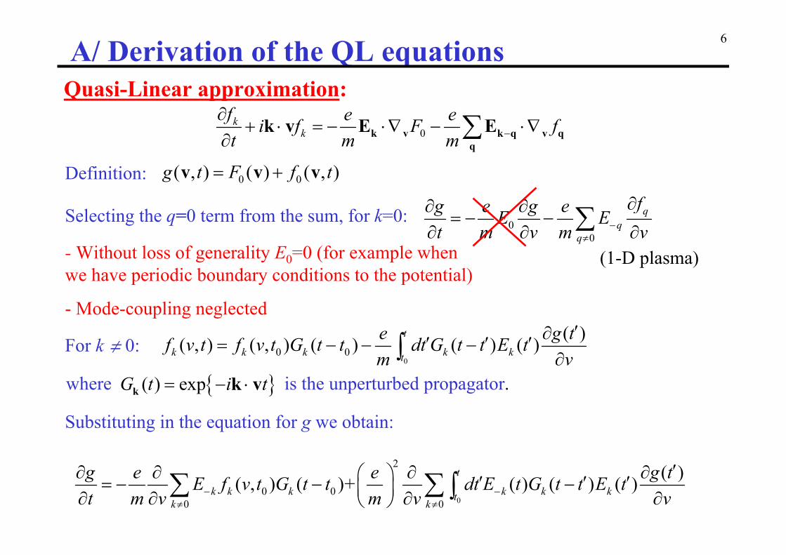
6A/ Derivation of the QL equationsQuasi-Linear approximation:

0k

kf e ei f F ft m m

k v k q v qq

k v E E

Definition: 0 0( , ) ( ) ( , )g t F f t v v v

Selecting the q=0 term from the sum, for k=0:

(1-D plasma)- Without loss of generality E0=0 (for example when we have periodic boundary conditions to the potential)

- Mode-coupling neglected

00

qq

q

fg e g eE Et m v m v

00 0

( )( , ) ( , ) ( ) ( ) ( )t

k k k k kt

e g tf v t f v t G t t dt G t t E tm v

For k ∫ 0:

Substituting in the equation for g we obtain:

0

2

0 00 0

( )( , ) ( )+ ( ) ( ) ( )t

k k k k k ktk k

g e e g tE f v t G t t dt E t G t t E tt m v m v v

where is the unperturbed propagator. ( ) expG t i t k k v

7A/ Assumptions of the standard QL theory

0

2

0 00 0

( )( , ) ( )+ ( ) ( ) ( )t

k k k k k ktk k

g e e g tE f v t G t t dt E t G t t E tt m v m v v

ASSUMPTIONS:

A1. For sufficiently large t-t0, the first term can be discarded, since positive and negative contributions from the rapidly oscillating (in kv) function Gk(t-t0) = exp[-ikv(t-t0)] cancel out in sums over k (phase mixing for wide spectra).

A2. The sum in the brackets corresponds to the autocorrelation of the electric field as seen by a free (unperturbed) particle

which decays with (t-t0) for turbulent or wide-spectrum electric fields. This justifies the Markovian evaluation of ∑g/ ∑v neglecting its time dependence (set t’ = t) when its relaxation time (τrel) is larger than the characteristic decay time of the autocorrelation of the fields (τac).Based on the same arguments the limit t0→ - ∞ is taken.

0 0 0( , , ) ( , ) ( ( ),x

C v t t E x t E x v t t t

( )g gD vt v v

Standard QL equation (Fokker-Planck, FP)

( ) (0) , ks tk k k k kE t E e s iω γ For we have:

8A/ Forms of the QL diffusion coefficient D

22 22

2 20

2( ) k kk

k kk k k

E γe eD v Em s ikv m ω kv γ

Bounded (periodic) plasmas – discrete wave spectra:

, k k k kω ω γ γ

-Difficulty in dealing with damped waves γk<0 due to negative diffusivity[Kaufman (1972), Fukai & Harris (1972)]

In the limit 0kγ

22

0

( ) 2 k kk

eD v π E δ ω kvm

only resonant particles included

Infinite plasmas – continuous wave spectra:1

2Lkdk

π

22 ( )( )

2 ( )k k

E ke dkD v im π ω kv iγ

In the limit , using Plemelj’s formula: 0kγ

includes both nonresonant and resonant particles

222( )

( ) P. ( ) ( )2 k

k

E ke dkD v i πδ ω kv E km π ω kv

9

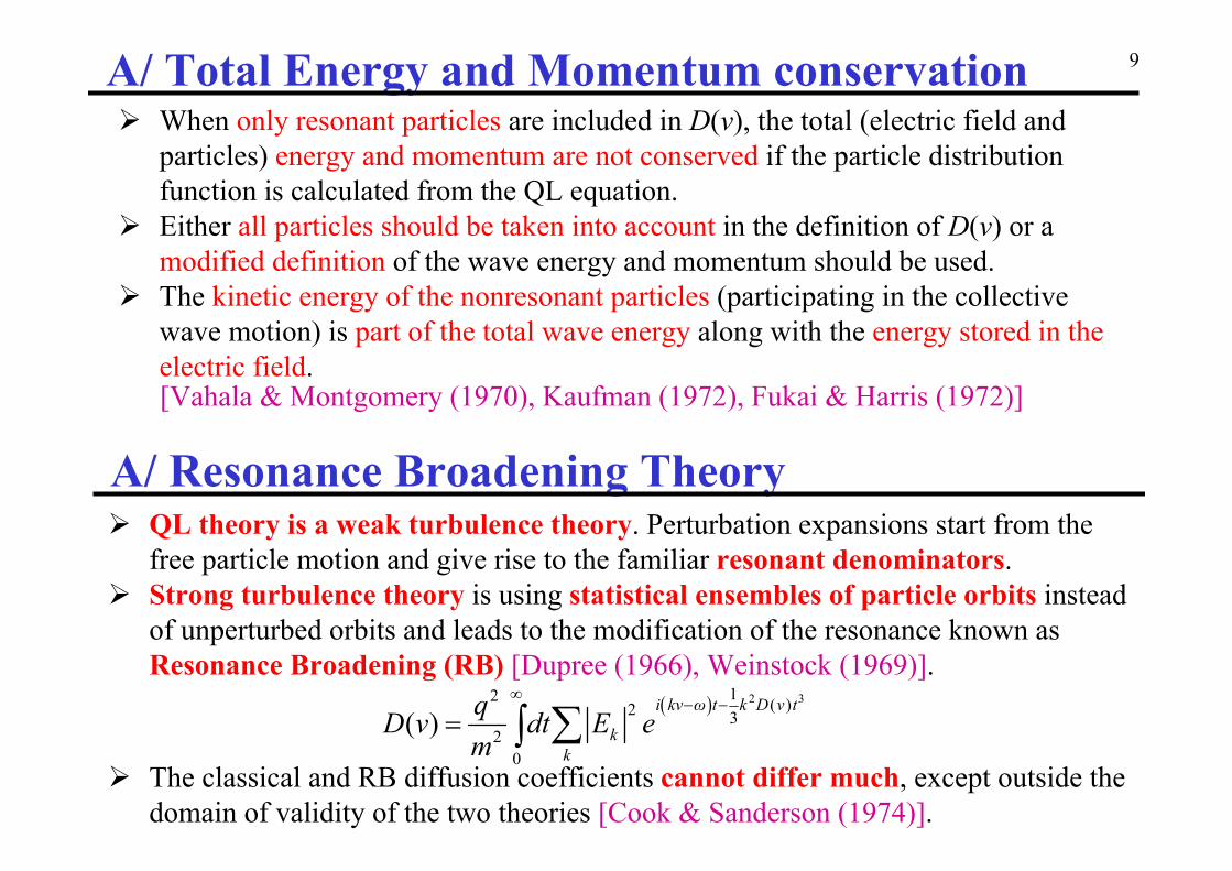
When only resonant particles are included in D(v), the total (electric field and particles) energy and momentum are not conserved if the particle distribution function is calculated from the QL equation.

Either all particles should be taken into account in the definition of D(v) or a modified definition of the wave energy and momentum should be used.

The kinetic energy of the nonresonant particles (participating in the collective wave motion) is part of the total wave energy along with the energy stored in the electric field.

A/ Total Energy and Momentum conservation

[Vahala & Montgomery (1970), Kaufman (1972), Fukai & Harris (1972)]

A/ Resonance Broadening Theory QL theory is a weak turbulence theory. Perturbation expansions start from the

free particle motion and give rise to the familiar resonant denominators. Strong turbulence theory is using statistical ensembles of particle orbits instead

of unperturbed orbits and leads to the modification of the resonance known as Resonance Broadening (RB) [Dupree (1966), Weinstock (1969)].

2 312 ( )2 32

0

( )i kv ω t k D v t

kk

qD v dt E em

The classical and RB diffusion coefficients cannot differ much, except outside the

domain of validity of the two theories [Cook & Sanderson (1974)].

10B/ Hamiltonian phase space dynamics The efficiency of a kinetic theory (QL/weak/strong turbulence theory) with

respect to the description of the evolution of the distribution function directly depends on its efficiency to describe the actual underlying particle dynamics.

Particle phase space dynamics, in most realistic cases, are characterized by complex motion in an inhomogeneous phase space where regular orbits coexist with chaotic orbits. In that case the dynamics are not stochastic (like Brownian motion) and statistical assumptions cannot be imposed.

In the following we utilize a well-studied system in order to discuss the phase space complexity and the applicability and validity of the standard QL theory.

Standard Map (Chirikov-Taylor)

Interaction of a charged particle with an infinite set of plane waves2

cos( )2 n

mvH qE kx nωt

The change in particle velocity and phase after every time step T = 2π/ω is

1

1 1

sin mod 2π mod 2π

n n n

n n n

p p K xx x p

( )2, , 2kx x kTv p qkE m Kp w =where

11B/ Standard Map: Poincare surfaces of section

K=0.5 K=0.97 K=5 Below a critical parameter K<Kc (left) the invariant Kolmogorov-Arnold-Moser

(KAM) curves restrict the variation of momentum p to be bounded.

The last invariant curve (rotation number = (◊5-1)/2, “golden mean”) is destroyed at Kg ≈ 0.97 (middle). This is a generic phase space structure typical for Hamiltonian systems: stability islands are embedded in a chaotic sea, similar structure appears on smaller and smaller scales.

Above the critical value K>Kc (right) we have a mixture of chaotic orbits and visible islands of stability and the variation of p becomes unbounded and is characterized by a “diffusive” growth.

12B/ Evolution of the distribution functionStarting from a Master Equation for the transition probabilities we obtain the Fokker-Planck equation:

( ) ( )( )f p f pD pn p p

2( )( )

2x

ΔpD p

Δnwith the diffusion coefficients defined as

What is to be taken as n and Δn?

For chaotic enough systems we expect that there exists a correlation “time” nc such that any reasonably smooth initial phase (x) distribution relaxes to a uniform phase distribution after nc steps.

Δn is a number of steps considerably larger than the correlation “time” nc

Due to typical co-existence of chaotic and regular (correlated) orbits ncdepends strongly on p and can be quite large for orbits close to regular due to stickiness effects.

cn Δn n

1 1 0: ( )( ) 0 for c n n n cxn C p p p p n n

13B/ Calculations of the diffusion coefficientSingle-step calculation (Δn=1)- corresponds to the Quasi Linear result- corresponds to a completely randomized motion

(Brownian motion) in the FP equation with DQL the time evolution

of f scales with K

2

4QLKD

Multi-step calculation (Δn>1)- corrections due to orbit correlations- D/DQL→1 for K→∞- oscillations in D due to increasingly

important effects of KAM curves and resonance islands for small K

- existence of non-diffusive orbits D does not depend on p so it cannot

take properly into account strong phase space inhomogeneity for finite K

2 2 22 1 2 3

12 ( ) ( ) ( ) ( )2QL

D J K J K J K J KD

QL

DD

K

Δnnum=50

[Rechester & White (1980)]

14

1central

resonance

v ω kΔv d

B/ Particle interaction with localized waves

2de

L

In the standard map we have an infinite number of modes with equal amplitude, so that the entire d.f. is affected.

In the case of localized waves we have a finite wave spectrum so that only part of the d.f. is affected.

2 220 cos( )x L dE E e kx ωt

[Fuchs, Krapchev, Ram & Bers (1985)]

15B/ Particle interaction with localized waves

2

2 2

12

( 2) 4

220

2 2 2 2

cos ( 1) cos

1,

1 , is the nearest integer to 2

mβ x L m βΜ

mm M

b

m

α πx αe x t e k x tL β

eE k ω Δkα βmω ω k d k

k m M M L π

Electron equations of motion

Characteristic time scales Autocorrelation time: the width of the field autocorrelation function as seen by

a particle or the transit time of the particle through the wavepacket

Trapping time: the shortest period of a particle oscillating around the minimum of the potential corresponding to a single Fourier mode

2acτ v β

2 2b

b

π πτ ω α

16B/ Particle interaction with localized waves

What does the condition (QL theory) imply for phase space dynamics?ac bτ τ

Only the nearest Fourier modes contribute to resonance wave-particle interaction to a point of the velocity space.

Condition for weak resonance overlap.

What is the case of phase space dynamics when ?ac bτ τ

The resonance overlap is so strong that a resonant particle sees a large number of Fourier modes at the same time. The particle sees the wave packet as a whole, rather than its individual Fourier components.

The complexity of the particle motion is a result of non-adiabatic separatrixcrossings during transitions from trapped to untrapped states and vice versa.

Nonresonant particles (bulk) are affected by a ponderomotive force.

17C/ General kinetic formulation of w-p interactionsA kinetic formulation of wave-particle interactions has to be based on calculations / estimations for the underlying particle dynamics.These can be performed on the basis of: Perturbation methods, such as in the case of weak turbulence theories, starting

from the free particle motion. Statistical estimations, taking into account estimations of ensemble averages of

the actual particle motion, such as in the case of strong turbulence theories.

We apply a systematic Canonical Perturbation Theory (CPT), utilizing Lie transform techniques in order to calculate particle orbits and directly connect these calculations with the evolution of the collective behavior as described by the d.f.

Standard applications of the CPT include: Calculation of approximate invariants of the motion (KAM curves) –

perturbation theory in the infinite time interval. Construction of Canonical Mappings for the calculation of actual particle orbits in

terms of symplectic integration schemes – perturbation theory in a finite time interval – the effective perturbation strength is proportional to the waveamplitude and the time step [Abdullaev (2002), Kominis et al, J. Phys. A (2008)].

18C/ Action-Angle Variables (unperturbed system)Unperturbed (integrable) system (to which we apply the CPT):Guiding center particle motion in an axisymmetric magnetic field

Action-Angle variables:

1 2 3

1 2 3

( , , ) ( , , )

( , , ) ( , , )P

g P

J J J J p

J

θ

J3= pφ

J2= JP

J1= μ

Action

Canonical angular momentumBanana center (magnetic surface )

Toroidal flux (drift surface)Toroidal flux (banana)

Magnetic moment

Circulating particlesTrapped particles

a

[Kaufman (1972)]

19C/ Non-Axisymmetric Perturbations

0 1( , ) ( ) ( , , )H t J θ J J θ( )

1( , , )

( , , ) ( )P g

i t

m m mt H e

mm θm

mJ θ J

Perturbed Hamiltonian:

Perturbations:

where γm is the growth rate of the perturbation

Resonance conditions (breaking of invariants): ωm= mPωP+mΦωΦ+mgωg

- Case (mg= 0) low frequency resonances

- Case (mg= 0, ωm= 0, mΦ∫ 0) magnetic islands

- Case (mg≠ 0) cyclotron-resonance (external rf fields: heating, current drive)

Study of the interplay of all kinds of perturbations

m m mω ω iγ

20C/ Lie transform method

0( ; ),f z t t t0 0( , )f z tHS

z Tz

0 0( , )f z tKS

0( ; ),f z t t t

1z T z

- SH: time evolution operator related to the Hamiltonian H

- For a θ-independent K, SK leaves the actions unchanged and evolves only θ1

0 0 0 0 0 0 0( ( ; ), ) ( , ) ( ; ) ( , ) ( , )Kf t t t T t S t t T t f tz z z z

Definitions:T=e-L, Lf=[w,f]

L, Lie operatorw, Lie generator (LG)[ , ], Poisson bracket

Properties of Lie transforms:- They generate canonical transformations- They commute with functions: f(Tz)=Tf(z)

[Kominis, Hizanidis, Constantinescu, Dumbrajs, J. Phys. A 41, 115202 (2008)]

21C/ Lie series perturbation methodDeprit’s series: - H, K, T, w: expanded in power series of the small parameter ε- T generates the identity transformation to zero order- At each order ε, LG is given by linear equations:

- Solutions in the finite time interval [t0, t]

where ω0(J) = ∑Η0/ ∑J are the unpertrubed frequencies and

( )0 ,

0, ( ) i ω tn

n nw w H P et

mm θm

mJ

0( ) ( )

( ),

0 ( )

m mi t i ti t

n nm

e ew P ei

0

Ω J Ω Jm θ ω J

mm

JΩ J

0( ) ( ) ω m mΩ J m ω J

Canonical Perturbation Theory in a finite time interval:

wn are nonsingular at resonant actions: m·ω0(J) – ωm= 0, even when γm= 0 (steady state)

The amplitude of wn (effective perturbation strength) is proportional to Δt=t-t0

The problem of small denominators does not appear

22C/ Reduction by angle-averaging- Transformation in the finite time interval [t0, t]:

- wn(z, t0) = 0 T(z, t0)=I, - SK(t ; t0)T-1(J0 ,θ0, t0) = T-1(J0 ,θ+Δθ,, t)

- For a partially averaged distribution function F:

where F is a function of the actions J, the remaining angles θ΄ and time t.

0

1( , ) , Δ ( , )t tf T f J θ J θ θ J θ

0

1( , ) ( , ) t tF T F θ

J θ J θ

10 0 0 0 0 0 0 0( ( ; )) ( , ) ( ; ) ( , ) ( , )

Kf t t T t S t t T t f tz z z z

Functional Mapping for finite Δt=t-t0

( , ) ( , ) F f θJ θ J θ

23C/ Hierarchy of Evolution Equations

- Dynamical reduction - Loss of information (“projection”)

Momentum and particle (radial) transport under the presence of high-frequency rf fields and nonaxisymmetric magnetic perturbations

6-D Vlasov’s equation

5-D (JP, pφ, μ, ΘP,Φ)

4-D (JP, pφ, μ, ΘP)

3-D Action diffusion equation

Averaging over the gyro-angle Θg(high-frequency perturbations)

Averaging over the toroidal angle Φ(non-axisymmetric perturbations)

Averaging over the poloidal angle ΘP

[Kominis, Ram, Hizanidis, Phys. Plasmas 15, 122501 (2008)]

24C/ Hierarchy of QL Evolution Equations1

2112

12

12

Τ Ι L L L Quasi Linear approximation:keep terms up to order ε2

0 0, , , , ,F t t F t t F t z z zz D z z C z z

, z J θ

By taking F=z and utilizing the properties of Deprit’s series we can show that:

1 1(1/ 2) (Δ ) (Δ ) θD z zwhere (Δz)1,2 is the first and second -order variations of z in the time interval Δt=t-t0

2(Δ ) θC z

FUNCTIONAL MAPPING

0 0,

, , , ,F t

t F t t F tt

z t z t z

zD z z C z z

EVOLUTION EQUATION

By differentiating we obtain:

where Dt, Ct are the time derivatives of D and C.

Note that in the r.h.s. we have F evaluated at time t0.

21 1 1

1 2 1 221 1 1

1 1 1, , , , , ,2 2 2

w w wt t w w w w

w w w

θ J θ θθθ J

θ θJ θ Jθ θ

D J θ C J θ

25C/ QL evolution of Action Distribution functions

22 2

2 20

2 22 2

0

1 2 cos ( ), , ( ) ,

2 ( )

1 cos ( ) ( ) sin ( ), , ( )

( )

γ Δt γ Δtγ t

γ Δt γ Δtγ t

e e Ω Δtt Δt H e

Ω γ

γ e Ω Δt Ω e Ω Δtt Δt H e

Ω γ

m m

m

m m

m

mm

m m m

m m m mt m

m m m

JD J mm J

J

J J JD J mm J

J

Only under the condition: we obtain a Fokker-Planck equation with nonsingular, time-varying tensor.

( , ) ( , )F t Δt F t J JJ J

nonsingular, time-varying operators 0 0( ) ( ) , Ω ω Δt t t m mJ m ω J

, , , ,F t t Δt F t Δt J JJ D J J FUNCTIONAL MAPPING

,, , ,t

F tt Δt F t Δt

t

J JJ

D J J EVOLUTION EQUATION

By averaging over all angles, we have C = Ct = 0 (due to the form of wn) and D, Dtare determined exclusively by the first order Lie generating function:

[Kominis, Ram, Hizanidis, Phys. Rev. Lett, 104, 235001 (2010)][Hizanidis, Kominis, Ram, Plasma Phys. Control. Fusion. 52, 124022 (2010) ]

26C/ Properties of the operator D (mapping)

20, 1 2γ tm

0γ m

0γ m

Δ ( ) 0,Ω tm J

t

2

0

22

2 2

, , ( ) Δ , , ; , ,

1 2 cos ( )Δ , , ; ,

2 ( )

γ Δt γ Δtγ t

t Δt H t Δt γ ω

e e Ω Δtt Δt γ ω e

Ω γ

m m

m

m m mm

mm m

m m

D J mm J J

JJ

J

( )Ωm J ( )Ωm J( )Ωm J

tt t

0γ m 0γ m 0γ mΔΔ Δ

Δ is nonsingular, smooth, time-dependent(acts on a wide action range, resonant & nonresonant)

Δ is positive for every t, J, for all γm(growing, damped and steady-state modes).

For γm→0 and t→+∞,

For γm<0 and t→+∞,

Δ δ ( )Ω m J

2 2Δ 1 2 ( )Ω γ m mJ

27

0, γ tm

0γ m

0γ m

Δ ( ) 0,t Ω tm J

t

( )Ωm J ( )Ωm J( )Ωm Jtt t

0γ m 0γ m 0γ mΔtΔt Δt

2

0

22 2

, , ( ) Δ , , ; , ,

1 cos ( ) ( ) sin ( )Δ , , ; ,

( )

t

γ Δt γ Δtγ t

t

t Δt H t Δt γ ω

γ e Ω Δt Ω e Ω Δtt Δt γ ω e

Ω γ

m m

m

t m m mm

m m m mm m

m m

D J mm J J

J J JJ

J

Δt is nonsingular, smooth, time-dependent (acts on a wide action range, resonant & nonresonant)

Δt can be initially (small t) negative for some values of J corresponding to nonresonant particles, for all γm (growing, damped and time-periodic modes).

For γm→0 and t→+∞,

For γm<0 and t→+∞,

Δ δ ( )t Ω m J

Δ 0t

C/ Properties of the operator Dt (evolution eq.)

28C/ Revised QL theory for the Action d.f.We have derived a Functional Mapping and an Evolution Equation governing the evolution of the Action d.f. under no statistical assumptions with the utilization of the CPT in finite time intervals.

What are the restrictions of the revised theory? Since there are no other assumptions, the only restrictions come from the validity

of our Perturbation Theory. The accuracy (μ) of the mapping is μ ~ Ετ2, whereτ = Δt is the time step and E the amplitude of the wave perturbation.

A sufficiently small time step τ ensures accuracy of the mapping even for larger wave amplitudes. The condition is

which can also be written in the equivalent form

where τb is the trapping time. The condition for the validity of the standard QL theory is obtained by τ → τac! This is due to the fact that in the context of standard QL theory, the perturbation method is applied for the infinite time interval and in that case the accuracy is

This explains the inapplicability of the standard QL theory to coherent waves and trapping effects.

1μ

bτ τ

2acμ Ετ

29

mΦ

1m mv k

α= 0.05, β=0.01

τac/τb=0.71/v

C/ Operators for a Gaussian wave spectrum

2( 2) cosβ x LΦ αe x t ( , )D v t

v

t

( , )tD v t

v

t

3( , 10 )D v t

v

3( , 10 )tD v t

v

Fourier Spectrum

Mapping Operator D

Evolution Equation Operator Dt

30C/ Obtaining the standard QL equations

Steps and assumptions for obtaining the standard QL equations:

1.The time scale of the evolution of the action d.f. (relaxation time, τrel) is short compared to the autocorrelation time (for which the sum over all modes in Dt takes significant values). => - A Fokker-Planck equation with a time-varying, nonsingular operator is

derived. - The operator acts on both resonant and nonresonant particles and can include both growing and damped modes.- The equation is time reversible.

2.=> - The operator becomes singular (sum of Dirac delta functions) and acts only

on exactly resonant particles (unphysical).- The singularity cannot be removed (in principle) for discrete wave spectra (bounded systems).- The equation becomes irreversible and describes a purely diffusive evolution.

,, , ,t

F tt Δt F t Δt

t

J JJ

D J J EVOLUTION EQUATION

( , ) ( , )F t Δt F t J JJ J

t

31SUMMARY & CONCLUSIONS Utilization of the Canonical Perturbation Theory in finite time intervals.

Rather than obtaining a diffusion coefficient (tensor), as in QL or RBT, we derive a functional mapping for the evolution of the angle-averaged d.f.

No statistical assumptions (ergodicity, mixing, memory loss) – derivation based on first principles (equations of motion).

The operators are time-dependent, nonsingular and incorporate both resonant and nonresonant particles – acting on wider areas of the phase space.

The distribution function evolves along with the particle motion, intermediate time scales can be taken into account. Transient effects included.

No time-scale separation based on phenomenological (Brownian motion, random walk) arguments on the underlying particle dynamics.

The method is applicable to coherent waves and takes into account trapping effects.

The accuracy of the method depends only on the time step which can be selected according to the amplitude, autocorrelation time and growth rate of the waves.

The resulting evolution of the d.f. can describe more complex processes than normal (or anomalous) diffusion.

32C/ Operators for a Gaussian wave spectrum

α= 0.05, β=0.1

τac/τb=0.22/v

2( 2) cosβ x LΦ αe x t

mΦ

1m mv k

( , )D v t

v

t

( , )tD v t

v

t

3( , 10 )D v t

v

3( , 10 )tD v t

v

Fourier Spectrum

Mapping Operator D

Evolution Equation Operator Dt