quantum physics - sri venkateswara college of … · why quantum physics? ... leading to the inside...

UNIT-III

QUANTUM PHYSICS

Black body radiation – Planck’s theory (derivation) – Deduction of Wien’s displacement law and Rayleigh – Jeans’ Law from Planck’s theory

Compton Effect-Theory and experimental verification – Properties of Matter waves – G.P Thomson experiment

Schrödinger’s wave equation – Time independent and time dependent equations – Physical significance of wave function – Particle in a one dimensional box

Electron microscope - Scanning electron microscope - Transmission electron microscope.

SYLLABUS

OBJECTIVESTo explain the principle of black body radiation and reveal the energy distribution in black body radiation

To derive Planck’s equation for radiation and explain the particle and wave nature (matter waves) of the quantum particles.

To derive de-Broglie equation related with momentum and wavelength of the particle.

To discuss the properties of the matter waves and explain the experimental evidence of matter waves.

To derive the Schrödinger wave equation for the motion of quantum application- particles a particle in one – dimensional box and its importance.

To study the principle, mechanism, applications of optical based instruments and operating the role of optical instruments and applications of optical microscope ,TEM and SEM

CONTENT

• Black body radiation

• Planck’s theory (derivation)

• Deduction of

- Wien’s displacement law

-Rayleigh – Jeans’ Law

from Planck’s theory

Why Quantum Physics?

• Classical mechanics (Newton's mechanics) and Maxwell's equations (electromagnetic theory) can explain MACROSCOPIC phenomena such as motion of billiard balls or rockets.

• Quantum mechanics is used to explain microscopic phenomena such as photon-atom scattering and flow of the electrons in a semiconductor.

• The behavior of a "microscopic" particle is very different from that of a classical particle:

– in some experiments it resembles the behavior of a classical wave (not localized in space)

– in other experiments it behaves as a classical particle (localized in space)

ORIGIN OF QUANTUM PHYSICS

BLACK BODY RADIATION

BLACK BODY RADIATION• Blackbody

• a cavity, such as a metal box with a small hole drilled into it.

• Incoming radiations entering the hole keep bouncing around inside the box with a negligible change of escaping again through the hole => Absorbed , the hole is the perfect absorber

• When heated, it would emit more radiations from a unit area through the hole at a given temperature => perfect emitter

BLACKBODY APPROXIMATION

• A good approximation of a black body is a small hole leading to the inside of a hollow object

• The hole acts as a perfect absorber

• The nature of the radiation leaving the cavity through the hole depends only on the temperature of the cavity

If the radiation emitted by a black body at a fixed temperature is analyzed by means of a suitable spectroscopic arrangement, it is found to spread up into a continuous spectrum.

The total energy is not distributed uniformly over the entire range of spectrum.

The distribution of energy in black body radiation for different wavelengths and at temperatures was determined experimentally by Lummer and Pringsheim.

The experiment arrangements are shown in figure.

ENERGY DISTRIBUTION OF SPECTRUM

Radiation fromblack body

Fluorspar prism

Bolometer

M1

M2



The radiation from the black body is rendered into a parallel beam by the concave mirror M1 . It is then allowed to fall on a fluorspar prism to resolve it into a spectrum.

The spectrum is brought to focus by another concave mirror M2 on to a linear bolometer.

The bolometer is connected to a galvanometer .

The deflection in the galvanometer corresponding to different are noted by rotating the prism table.

Then curves are plotted for energy verses wavelength . The experiment is done with the black body at different temperatures.

• Intensity of radiation increases with respect to increase in wavelength and at a particular wavelength it is maximum and after that it decreases

• As the temperature increases, the peak wavelength emitted by the black body decreases.

• At each temperature the black body emits a standard amount of energy. This is represented by the area under the curve.

• As temperature increases, the total energy emitted increases, because the total area under the curve increases.

• It also shows that the relationship is not linear as the area does not increase in even steps. The rate of increase of area and therefore energy increases as temperature increases.


PLANK’S THEORY

PLANK’S THEORY

Planck’s theory:

A black body contains a large number of oscillating particles:Each particle is vibrating with a characteristic frequency.

The frequency of radiation emitted by the oscillator is the same as the oscillator frequency.

The oscillator can absorb energy in multiples of small unit called quantum.This quantum of radiation is called photon.

The energy of a photon is directly proportional to the frequency of radiation emitted.

An oscillator vibrating with frequency can only emit energy in integral multiples of h. , where n= 1, 2, 3, 4…….n. n is called quantum number.

PLANK’S QUANTUM THEORY OFBLACK BODY RADIATION

PLANCK’S LAW OF RADIATION

The energy density of radiations emitted by a black body at a temperature T in the wavelength range to +d is given by

h =6.625x10-34Js-1 - Planck’s constant.

C= 3x108 ms-1 -velocity of light

K = 1.38x 10-23 J/K -Blotzmann constant

T is the absolute temperature in kelvin.

DERIVATION OF PLANCK’S LAW

Consider a black body with a large number of atomic oscillators.Average energy per oscillator is

E is the total energy of all the oscillators and N is the number of oscillators.

Let the number of oscillators in ground state is be N0.According to Maxwell’s law of distribution, the number of oscillators having

an energy value EN is given by

T is the absolute temperature. K is the Boltzmann constant.

Let N0 be the number of oscillators having energy E0,

– N1 be the number of oscillators having energy E1,

– N2 be the number of oscillators having energy E2 and so on.

Then

From Planck’s theory, E can take only integral values of h.Hence the possible energy are 0, h, 2h,3 h……. and so on.


Putting

( using Binomial expansion)


The total energy

Substituting the value of

Putting


Substituting (11) and (7) in (1)


Substituting the value for x

The number of oscillators per unit volume in the wavelength range and +d is given by


Hence the energy density of radiation between the wavelength range and +d is

Ed = No. of oscillator per unit volume in the range and +d X Average energy.


The equation (16) represents Planck’s law of radiation.

Planck’s law can also be represented in terms of frequencies.


1. Wien’s Law:

1. Wien’s law holds good when wavelength is small.( is large)

2. Therefore and is very large compared to 1.

3. Neglecting 1 in equation (16)

4. Equation (18) represents Wien’s law.

Thus Planck’s law reduces to Wien’s law at shorter wavelength.

DEDUCTION OF RADIATION LAWS FROM PLANCK’S LAW

2.Raleigh- Jean’s law:

1. Raleigh- jean’s law holds good when wavelength is large.( is small).

2. Therefore and expanding we get (1+

3. Substituting in (16)

Thus Planck’s law reduces to Raleigh- jean’s law at longer wavelength.


1. It explains the energy spectrum of the black body radiation.

2. It is used to deduce Wien’s displacement law and Rayleigh-Jean’s law.

3. It introduces a new concept, i.e., energy is absorbed or emitted in a discrete manner in terms of quanta of magnitude of hν i.e.,

ADVANTAGES OF PLANCK’S THEORY

E = nhν

CONTENT

• Compton Effect

• Compton theory (derivation)

• Compton experimental verification

• Properties of Matter waves

• G.P Thomson experiment from Planck’s

theory

PHOTON AND ITS PROPERTIES

PHOTON AND ITS PROPERTIES The term photon was coined by Gilbert Lewis in 1926. A photon is the quantum of light and all other forms of electromagnetic radiation. It exhibits dual nature (acts as a wave and as a particle)..

They are discrete energy values emitted as small pockets/bundles/quantas by the source. They possess definite frequency/wavelength.

According to Planck, the exchange of energy between light and matter is not continuous, but it is in the form of packets or quanta of definite energy proportional to frequency of light.

E ∝ ν

E = hν where the packets of energy hν is called Photon.

Two Kinds:Coherent scattering or classical scattering or Thomson scatteringIncoherent scattering or Compton scattering

Coherent scattering:

X rays are scattered without any change in wavelength.Obeys classical electromagnetic theory

Compton scattering:

Scattered beam consists of two wavelengths.

One is having same wavelength as the incident beam

The other is having a slightly longer wavelength called modified beam.

SCATTERING OF X-RAYS

COMPTON EFFECT

(i) Modified radiation – having lower frequency or larger wavelength

(ii) Un Modified radiation – having same frequency or wavelength

This change in wavelength of the scattered X rays is known as the Compton shift.

This effect is called Compton Effect.

A beam of monochromatic radiation (x-rays, γ-rays) of high frequency fall on a low atomic no. substance( carbon, graphite),the beam is scattered into two components.

• Compton treated this scattering as the interaction between X ray and the matter as a particle collision between X ray photon and loosely bound electron in the matter.

• Consider an X ray photon of frequency striking an electron at rest.

• This Photon is scattered through an angle to x-axis.

• Let the frequency of the scattered photon be ’.

• During collision the photon gives energy to the electron.

• This electron moves with a velocity V at an angle to x axis.

THEORY OF COMPTON EFFECT

Total Energy before collision:Energy of the incident photon

Energy of the electron at rest

where m0 is the rest mass of electron and C the velocity of light.

Therefore total energy before collision

Total energy after collision:Final energy of the photon

Energy of the electron at rest

where m0 is the rest mass of electron and C the velocity of light.

Therefore total energy before collision


Before Collision After Collision

Energy of Incident photon = hγ Energy of scattered photon = hγ’

Energy of electron, at rest = m0C2 Energy of recoiled

electron

=

mC2

Total Energy = hγ + m0C2 Total Energy = hγ’ + mC2

By the law of conservation of energy Total energy before collision = Total energy after collision


Total momentum along x axis before collisionInitial momentum of photon along x axis

Initial momentum of electron along x axis = 0

Total momentum before collision along x axis

Total momentum along x axis after collisionThe momentum is resolved along x axis and y axis.

Final momentum of momentum along x axis

Final momentum of electron along x axis

Total final momentum along s axis


Momentum calculation before collision



Momentum of Incident

photon

=

hγ/C

Momentum of scattered

photon

=(hγ’/C) cosθ

Momentum of electron, at

rest

= 0 Momentum of recoiled

electron

= mv cosϕ

Total Momentum = hγ/C Total Momentum = (hγ’/C) cosθ + mv

cosϕ

, Applying the law of conservation of momentumMomentum before collision = momentum after collision


Momentum calculation after collision


Total momentum along y axis before collision

Initial momentum of photon along y axis =0

Initial momentum of electron along y axis = 0Total momentum before collision along y axis= 0

Total momentum along y axis after collision

Final momentum of photon along y axis

Final momentum of electron along y axis

( along the negative Y direction)

Total momentum after collision along y axis


Applying the law of conservation of momentumMomentum before collision = momentum after collision


Momentum of Incident

photon

= 0 Momentum of

scattered photon

= - (hγ’/C) sinθ

Momentum of electron,

at rest

= 0 Momentum of

recoiled electron

= mv sin ϕ

Total Momentum = 0 Total Momentum = - (hγ’/C) sinθ + mv

sin ϕ


Squaring (3) and (4) and adding,

LHS of the equation RHS of the equation

=

=

=

=


Equating LHS and RHS,

Squaring (1) ,

Eqn (8)- eqn (6)


From the theory the variation of mass with velocity is given by

Squaring (10)


Multiplying on both sides by C2

Substituting in (10)


Multiplying by C on both the sides,

Therefore the change in wavelength is given by

The change in wavelength d does not depend on the(i) wavelength of the incident photon

(ii) Nature of the scattering material The change in wavelength d depends only on the

scattering angle.


Case (1) When =0 then,

Case (2) When =90o then,

Substituting the values for h,m0 and C

Case(3) When =180o then,

The change in wavelength is maximum at 1800


EXPERIMENTAL VERIFICATION OF COMPTON EFFECT

1. The experimental set up is as shown in the fig.

2. A beam of mono chromatic X ray beam is allowed to fall on the scattering material.

3. The scattered beam is received by a Bragg spectrometer.

4. The intensity of the scattered beam is measured for various angles of scattering.

5. A graph is plotted between the intensity and the wavelength.


6. Two peaks were found.

7. One belongs to unmodified and the other belongs to the modified beam.

8. The difference between the two peaks gives the shift in wavelength.

9. When the scattering angle is increased the shift also gets increased in accordance with

10. The experimental values were found to be in good agreement with that found by the formula.

11. Compton’s results at the scattering angles 0, 45 ◦, 90 ◦ and 135◦, are shown in the following Figure.


The wavelength of the scattered X -rays becomes longer as the scattering angle increases.

Compton shift λ is zero when θ = 0 Compton shift is maximum when θ = 135◦.


MATTER WAVES

De Broglie’s Hypothesis:

Waves and particles are the modes of energy propagation.

Universe of composed of matter and radiations.

Since matter loves symmetry matter and waves must be symmetric.

If radiation like light which is a wave can act like particle some time, then materials like particles can also act like wave some time.

Matter has dual wave particle nature. According to de Broglie hypothesis

The energy of the particle with quantum concept is

DE- BROGLIE WAVES AND WAVELENGTH

DE- BROGLIE WAVES AND WAVELENGTHFrom Planck’s theory

According to Einstein’s theory,

Equation (1) and (2)

Therefore

Where p is the momentum of the particle.

We know that Kinetic energy

Multiplying by m on both sides

Substituting in (4)

DE -BROGLIE WAVELENGTH INTERMS OF ENERGY

G.P. THOMSON’S EXPERIMENT

In 1927, George P. Thomson to demonstrate a diffraction pattern characteristic of the atomic arrangements in a target of powdered aluminum.

EVIDENCE OF DE- BROGLIE WAVES

G.P Thomson’s apparatus for the diffraction of electrons


diffraction patterns

A narrow beam of electrons is produced by the cathode C.

the beam is accelerated by potentials up to50kV.

These electrons rays after passing through a slit S are incident on a thin foil G of about thickness in the order of 10-6.

The diffraction of the electrons takes place at G and the patterns is photographed using the photographic plate P.

The diffracted electrons produce the diffraction rings asshown in diagram.


This patterns confirms that electrons are diffracted only due to the presence of electron and not due to secondary X-rays produced by the electrons while going through the foil G.

For example, if the foil G is removed, the entire pattern disappears. So, foil G is essential for the diffraction patterns.

Thus, the experiment clearly demonstrates the electrons behave aswaves, and the diffraction patterns can be produced only by the waves.

By knowing the ring diameter and the de Broglie wavelength of electrons the size of the crystal unit cell can be calculated.

The experimental result and its analysis are similar to those of powdered crystal experiment of X-ray diffraction.


• Schrödinger’s wave equation

• Time independent equations

• Time dependent equations

• Physical significance of wave function

• Particle in a one dimensional box

CONTENT

HEISENBERG PRINCIPLE

WAVE FUNCTION AND ITS SIGNIFICANCE Waves represent the propagation of a disturbance in a medium.

We are familiar with light waves, sound waves, and water waves.

These waves are characterized by some quantity that varies with position and time.

Since micro particles exhibit wave properties, it is assumed that a quantity represents de Broglie waves.

According to Heisenberg uncertainty principle , we can only know the possible value in a measurement.

The probability cannot be negative.

cannot be a measure of the presence of the particle at the location (x, y , z).

PHYSICAL SIGNIFICANCE OF WAVE FUNCTION

The wave function has no physical meaning.

It is a complex quantity representing the matter wave of a particle.

│ψ │2 = is real and positive, amplitude may be positive or negative but the intensity(square of amplitude) is always real and positive.

│ ψ │2 represents the probability density or probability of finding the particle in the given region.

For a given volume dτ, probability P = ∫ ∫ ∫│ ψ │2 dτ where dτ=dx dy dz

The probability value lies between 0 and 1.

∫ ∫ ∫│ ψ │2 dτ = 1, this wave function is called normalized wave function.

SCHRODINGER'S WAVE EQUATION

Austrian scientist, Erwin Schrodinger

describes the wave nature of a particle , derived in mathematical form

connected the expression of De-Broglie wavelength with classical wave equation

two forms of Schrodinger's wave equation

Time Independent wave equation

Time dependent wave equation

Schrodinger equation is basic equation of matter waves.

The two forms of the wave equation are:

Time independent wave equation

Time dependent wave equation

SCHRODINGER'S WAVE EQUATION

Let us consider a system of stationary wave associated with a moving particle.

Let φ be the wave function of the particle along x, y and z coordinatesaxes at any time t.

A particle can behave as a wave only under motion. So, it shouldaccelerated by a potential field.

The total energy (E) of the particle is equal to the sum of its potential energy (v) and kinetic energy.

SCHRODINGER'S TIME DEPENDENT WAVE EQUATION

(p=mv)


According to classical mechanics, If x is the position of the particle moving with the velocity v then the displacement of the particle at any time t is given by

Where ω is the Angular frequency ω= (6)becomes

If the v is the velocity of the particle behaving as a wave, then the frequency,


Substitute the value of Quantum operator


Differentiating eqn 13 partially with respect to “x” we get,

Differentiating once again eqn 13partially with respect to “x” we get

Since

we can write the (15) eqn as


Differentiating eqn 13partially with respect to “t” we get,


Equation (19) represents the one dimensional (along x direction) schroedinger wave equation. The wave function depends both on position (x,y,z) and time t.

Substituting Equations (16) and (18),in eqn (5) we get,


In Schroedinger time dependent wave eqn the wave function ψ depends on time , in Schroedinger time independent wave eqn ψ does not depends on time and hence it has many applications.

Splitting the RHS of this equation into two parts,

• Time dependent factor

• Time independent factor

SCHRODINGER'S TIME INDEPENDENT WAVE EQUATION

Where ψ represents the time independent wave function

Differentiating eqn 1partially with respect to “t” we get,


Differentiating eqn 1 partially with respect to “x” we get,

Differentiating eqn 1 once again partially with respect to “x” we get,

We know Schroedinger time dependent wave eqn

Substituting Eqn (1), (2), (3) in eqn (19)


Equation (10 ) represents the one dimensional schroedinger time independent

wave equation, because in this equation the wave function ψ is

independent of time.


PARTICLE IN A ONE DIMENSIONAL BOX

Boundary conditions:

V(x) = 0 when 0 x a

V(x) = when 0 x a

To find the wave function of a particle with in a box of width “a”, consider a Schrodinger’s one dimensional time independent wave eqn.

Since the potential energy inside the box is zero (V=0). The particle has kinetic energy alone and thus it is named as a free particle or free electron.For a free electron the schroedinger wave equation is given by


Eqn (3) is a second order differential equation, therefore it should have The solution with two arbitrary constants. The solution of the equation (3) isgiven by

Boundary condition at x=0, equation (5) becomes

We know

Comparing these two equations, we ca get

Boundary condition at x=l, equation (5) becomes


Energy of the particle (Eigen value)

K2 =

K2 =


Energy of the particle (Electron)


When n = 1

When n = 2

When n = 3

For each value of n,( n=1,2,3..) there is an energy level.

Each energy value is called Eigen value and thecorresponding wave function is called Eigen function.


Normalization of the wave function Normalization is the process by which the probability of finding the particle

is done. If the particle is definitely present in a box, then P=1


Energy levels with respect to (a) wave functions and (b) probability density

Therefore, the normalized wave function is given as,


• En is known as normalized Eigen function. The energy E

• normalized wave functions n are indicated in the above figure.


+

+

ELECTRON IN A CUBICAL METAL PIECE

DEGENERACY AND NON-DEGENERACYDegeneracy

When different quantum states of particle have the same energy Eigenvalue but different Eigen functions and quantum states are said to exhibit degeneracy the quantum states are called degenerate states.

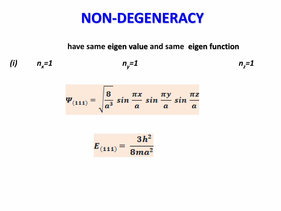
have same eigen value and same eigen function

(i) nx=1 ny=1 nz=1

NON-DEGENERACY

Degenerate energy states – have same eigen value but different eigen

function

(i) nx=1 ny=1 nz=2

(ii) nx=1 ny=2 nz=1

(iii) nx=2 ny=1 nz=1

the above equations are same Eigen value Eigen function.

DEGENERACY

MICROSCOPES

• Electron microscope

• Scanning electron microscope

• Transmission electron microscope.

CONTENT

BASIC TECHNICAL TERMS OF A MICROSCOPE

Microscope

• a device used to view the magnified image of a smaller object

Magnification Power

• ability of the microscope to show the image of an object in an

enlarged manner

Resolving Power

• ability of an instrument to form a distinct and separable images

of two point objects which are close to each other.

The resolving power is inversely proportional to wavelength.

“Microscope is a device used to view the magnified image of a smallerobject, which cannot be seen through a naked eye”.

TYPES OF ELECTRON MICROSCOPES

Transmission electron

microscope (TEM)

Scanning electron microscope (SEM)

Scanning transmission electron microscope

(STEM)

Electron Microscope

ELECTRON MICROSCOPE

Invention:

Electron microscope is a marvellous invention. It opensmany doors of nano science and technology.

The electron microscope was invented by the German scientists Ernst Bruche and Max Knoll of the Technical University of Berlin in 1931. The first practical electron

microscope was constructed by James Hiller and Albert Prebus of theUniversity of Toronto.

ELECTRON MICROSCOPE

Principle:A stream of electrons are passed through the object and the electrons

which carries the information about the object are focused by electric and magnetic fields. Since the resolving power is inversely proportional to the m wavelength,

the electron microscope has high resolving power because of its short wavelength.

Construction:The electron microscope is as shown in Figure and the wholearrangement is enclosed inside a vacuum chamber.

Electron microscope consists of the following:

(i) Electron gun (to produce stream of electrons),(ii) Magnetic lenses (for focusing),(iii) Fluorescent screen.

ELECTRON MICROSCOPE

ELECTRON MICROSCOPE

Working:

Stream of electrons are produced and accelerated by the electron gun.

Using magnetic condensing lens, the Accelerated electron beam is focused on the object.

Electrons are transmitted in the rarer and denser region of the object.

Electrons are absorbed in the denser region, The transmitted electron beam falling over the magnetic objective lens resolves the structure of the object.

The image can be magnified by the projector lens and obtained on fluorescent screen.

ELECTRON MICROSCOPE

Advantages:

Produces magnification as high as 105.

Applications:

To study the structure of bacteria, virus, etc.

To study the structure of the crystals, fibers.

To study the surface of metals.

To study the composition of paper, paints, etc.

ELECTRON MICROSCOPE

TRANSMISSION ELECTRON MICROSCOPE

Principle

Accelerated primary electrons are made to pass through the specimen.

The image formed by using the transmitted beam or diffracted beam.

The transmitted beam produces bright field image

The diffracted image is used to produce dark field image.


Construction:

Electron gun:

Electron gun produces a high energy electron beam by thermionic emission.These electrons are accelerated by the anode towards the specimen

Magnetic condensing lens:

These are coils carrying current.

The beam of electrons passing between two can be made to converge or diverge.The focal length can be adjusted by varying the current in the coils

The electron beam can be focused to a fine point on the specimen.


Magnetic projector lens:

The magnetic projector lens is a diverging lens.It is placed in before the fluorescent screen

Fluorescent ( Phosphor) screen or Charge coupled device (CCD):

The image can be recorded by using florescent or Phosphor or charge coupled device.


Working:

The electron beam produced by the electron gun is focused on the specimen.

Based on the angle of incident the beam is partially transmitted and partially diffracted.

Both the beams are combined to form phase contrast image.

The diffracted beam is eliminated to increase the contrast and brightness.

At the E-wald sphere, both the transmitted beam and the diffracted beamsare recombined. The combined image is called the phase contrast image.


Bright field Dark field image


Bright Field Image:

The image obtained due to the transmitted beam alone (i.e., due to the elastic scattering) is called bright field image.

Dark Field Image:

The image obtained due to the diffracted beam alone (i.e., due to theinelastic scattering) is called dark field image.

Using the transmitting beam, an amplitude contrast image has to beobtained. The intensity and contrast of this image is more.

The bright field image and dark field image is shown in Figure

The magnified image is recorded in the florescent screen or CCD.


Advantages:High resolution image which cannot be obtained in optical microscope.

It is easy to change the focal length of the lenses by adjusting the current.

Different types of image processing are possible.

Limitations:TEM requires an extensive sample preparation.

The penetration may change the structure of the sample.

Time consuming process.

The region of analysis is too small and may not give the characteristic of the entire sample.

The sample may get damaged by the electrons.


Applications:

It is used in the investigation of atomic structure and in various field of science.

In biological applications, TEM is used to create tomographic reconstruction of small cells or a section of a large cell.

In material science it is used to find the dimensions of nanotubes.Used to study the defects in crystals and metals.

High resolution TEM (HRTEM) is used to study the crystal structure directly.


SCANNING ELECTRON MICROSCOPE (SEM)

Principle: Accelerated primary electrons are made to strike the object.

The secondary electrons emitted from the objects are collected by the detector to give the three dimensional image of the object.

Construction:1. Electron gun:

This produces a high energy electron beam by thermionic emission

These electrons are accelerated by the anode towards the specimen.2. Magnetic condensing lens: These are coils carrying current.

The beam of electrons can be made to converge or diverge.

The focal length can be adjusted by varying the current in the coils

The electron beam can be focused to a fine point on the specimen.


3. Scanning coil:This coil is placed between the condensing lens and the specimen.

This is energized by a varying voltage.

This produces a time varying magnetic field.

This field deflects the beam and the specimen can be scanned point by point.

4. Scintillator: This collects secondary electrons and converts into light signal.

5. Photomultiplier:The light signal is further amplified by photomultiplier.

6.CRO:Cathode ray oscilloscope produces the final image.


Working:

The primary electrons from the electron gun are incident on the sample after passing through the condensing lenses and scanning coil.

These high speed primary electrons falling on the sample produce secondary electrons.

The secondary electrons are collected by the Scintillator produces photons.

Photomultiplier converts these photons into electrical signal.

This signal after amplification is fed to the CRO, which in turn produces the amplified image of the specimen.


Advantages:

SEM can be used to examine large specimen.

It has a large depth of focus.

Three dimensional image can be obtained using SEM.

Image can be viewed directly to study the structural details.

Limitations:

The resolution of the image is limited to 10-20 nm and hence it is poor


Applications:

SEM is used to study the structure virus, and find the method to destroy it.It is used in the study of bacteria.

Chemical structure and composition of alloys, metals and semiconductors can be studied.

SEM is used in the study of the surface structure of the material.


DIFFERENCE BETWEEN OPTCAL AND ELECTRON MICROSCOPE

S.No Optical Microscope Electron Microscope

1 Photons are used Electrons are used

2Optical lenses are used

Lenses are formed by electrostatic and

magnetic fields

3Focal length of an optical lens is fixed

Focal length of an electron lens can be

changed

4 It depends upon the radius of curvature of

the lens

It depends on the strength of the field

and the velocity of an electron

5

Magnification up to 1000 times

Magnification is too high

- One million times in EM

- Three million times in SEM

- Ten million times in TEM

6 It gives only 2-dimensional effect It gives three dimensional effect

7It does not require vacuum

Electron microscope must be kept in

a highly vacuum

8Resolving power is low

Resolving power is high

s.No

SEM TEM

1 Scattered electrons are used Transmitted electrons are used

2 SEM provides a 3D image TEM provides an detailed image of a

specimen

3 Magnification upto 2 million times Magnification upto 50 million times

4Preparation of sample is easy Preparation of sample is difficult

5 Thick specimen can also be

analysed

The specimen should be thin

6 SEM is used for surface analysis TEM is used for analyzing sections

DIFFERENCE BETWEEN SEM AND TEM

Classical theory failed to explain the behavior of electrons (atomic particles).

Quantum theory was successful in explaining tiny particles, black body radiation, photo electric effect, Compton effect etc.

In 1990, max Planck proposed a theory to explain Block Body Radiation & BB spectrum it is known as quantum theory of radiation.

Quantum theory based on Heisenberg’s uncertainty principle and Bohr’s complementary principle.

Einstein explained the photo electric effect using Plank’s quantum theory.

When highly energetic fast moving electrons are stopped by a targetcontinuous spectrum of X -rays of all wavelengths are produced.

Quantum Physics at a Glance

When a beam of monochromatic X -rays strikes a target, X -rays will be scattered in all possible directions. The scattered X -rays consists of a longer wavelength in addition to original wavelength.

The change in wavelength in due to loss of energy in the incident X -rayphoton. This effect is called as Compton Effect.

Light is showing dual nature (i.e.) wave and particle nature. State of a quantum particle is explained by wave function (x, y, z, t).

Heisenberg uncertainty principle, it is impossible to determine simultaneously the position and momentum of a quantum particle with infinite precision x.p ≥ h

Schrodinger wave equation explains the wave nature of a particle inmathematical form. Time dependent equation.

Quantum Physics at a Glance

FORMULAE

De-BroglieWavelength

Change in wavelength

Wavelength of scattered radiation

Energy

Momentum

quantum physics - sri venkateswara college of … · why quantum physics? ... leading to the inside...

Documents