quantum monte carlo calculations of nuclear matter · quantum monte carlo calculations of nuclear...

Quantum Monte Carlo calculations of nuclear matter

Kevin E. SchmidtDepartment of PhysicsArizona State University

Work done with:Mohamed Bouadani, Arizona StateStefano Gandolfi, SISSAAlexei Illarionov, SISSAFrancesco Pederiva, TrentoStefano Fantoni, SISSA

Supported by the National Science Foundation

Arizona State University

Outline of Talk

• Introduction

• The nuclear Hamiltonian.

• Diffusion Monte Carlo.

• Spin sampling with auxiliary field diffusion Monte Carlo method.

• Fixed Phase Approximation

• Results

• Future


Introduction

We want to be able to predict the structure of nuclei and nuclear andneutron matter.

I will talk only about ground states.

Here the Hamiltonian will be for nonrelativistic protons and neutronsinteracting with a potential (mostly local).

Monte Carlo calculations need to be able to sample the nonlocal parts ofthe propagator.


Hamiltonian

The Hamiltonian is

H =∑i

p2i

2mi+

∑i<j

M∑p=1

vp(rij)O(p)(i, j) + V3

• i and j label the two nucleons

• rij is the distance separating the two nucleons

• O(p) include central, spin, isospin, and spin orbit operators, and M isthe maximum number of operators ( i.e. 18 in Argonne v18 model).

For our calculations we use:

For purely neutron systems the Argonne v′8 and the Urbana or Illinoisthree-body potentials

For nuclei and nuclear matter, we have used the Argonne v′6 potential. Weare working on including spin-orbit or three-body potentials.


The most important parts of the Urbana and Illinois three-body potentialsfor nuclei have a two-body spin structure and can be included easily. Theother parts can sometimes be done perturbatively, but need to be donecorrectly to give accurate results.

The operator terms in Argonne v′8 are∑p

v(rij)O(p)ij = vc(rij) + vτ(rij)~τi · ~τj

+vσ(rij)~σi · ~σj + vστ(rij)~σi · ~σj~τi · ~τj+vt(rij)tij + vtτ(rij)tij~τi · ~τj+vLS(rij)(~Li − ~Lj) · (~Si + ~Sj)

+vLSτ(rij)(~Li − ~Lj) · (~Si + ~Sj)~τi · ~τj


The central Part can be handled using standard GFMC or DMC.

The most successful method for light nuclei uses Monte Carlo for thespatial variables and complete summation over the spin-isospin states.

The number of good Sz Tz spin-isospin states is

A!Z!(A− Z)!

2A

which can be lowered by a small factor if good T 2 states are constructed.

The exponential growth of these states limits this brute force method to12C at present.


Diffusion Monte Carlo for Central PotentialsSchrodinger equation in imaginary time (measured in units of energy−1) isthe diffusion equation

(H − ET )Ψ(R, t) =[− h2

2m∇2 + V (R)− ET

]Ψ(R, t) = − ∂

∂tΨ(R, t)

Formal solution

Ψ(R, t) = e−(H−ET )tΨ(R, 0)

HΨn(R) = EnΨn(R)

Ψ(R, 0) =∑n

anΨn(R)

Ψ(R, t) = e−(E0−ET )ta0Ψ0(R) +∑n 6=0

e−(En−E0)tanΨn(R)

Result converges to the lowest energy eigenstate not orthogonal toΨ(R, 0).


Schematic Implementation

Ψ(R, t+ ∆t) =∫dR′e−(V (R)−ET )∆t〈R|e−P2

2m∆t|R′〉Ψ(R′, t)

• A particles (in a periodic box for matter).

• Use a short time approximation for the Green’s function.

• Sample gaussian for the kinetic energy term, evaluate the diagonalpotential terms as a weight.

• Use branching to control population.

• Use importance sampling to improve variance.

• For Fermions the wave function changes sign. Use fixed node ortransient estimation.


Monte Carlo Spin Sampling

We want to sample the spin and isospin.

In the usual p↑, p↓, n↑, n↓ basis.

R ≡ 3A x, y, z coordinates for the nucleons

S ≡ A discrete values selecting one of p↑, p↓, n↑, n↓

ΨT (R,S) = Trial wavefunction - a complex number for given R and S.

HS,S′(R) = the Hamiltonian

There are roughly 4A spin-isospin states. We could sample them with lowvariance if we could calculate ΨT (R,S) efficiently.

All known nontrivial trial functions require order 4A operations to calculateeither 1 or all the spin states.

We use trial functions with no spin-isospin operator correlations.


Sampling with an Auxiliary Field

We diagonalize the interaction in spinor space.

This requires Order(A3) operations – same complexity as determinant.

For A particles, the v6 interaction can be written as

V =∑i<j

[6∑p=1

vp(rij)O(p)(i, j)] = Vc + Vnc

= Vc +12

∑i,α,j,β

σi,αA(σ)i,α,j,βσj,β

+12

∑i,α,j,β

σi,αA(στ)i,α,j,βσj,β~τi · ~τj

+12

∑i,j

A(τ)i,j ~τi · ~τj


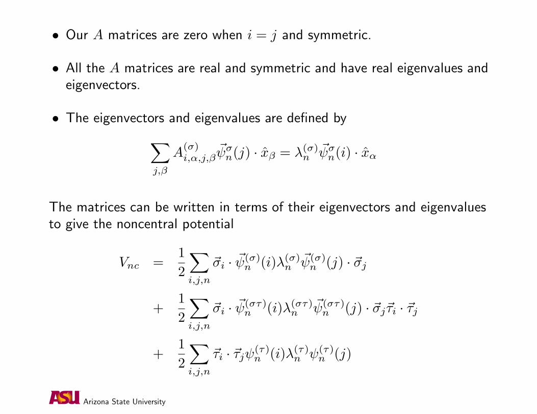
• Our A matrices are zero when i = j and symmetric.

• All the A matrices are real and symmetric and have real eigenvalues andeigenvectors.

• The eigenvectors and eigenvalues are defined by∑j,β

A(σ)i,α,j,β

~ψσn(j) · xβ = λ(σ)n~ψσn(i) · xα

The matrices can be written in terms of their eigenvectors and eigenvaluesto give the noncentral potential

Vnc =12

∑i,j,n

~σi · ~ψ(σ)n (i)λ(σ)

n~ψ(σ)n (j) · ~σj

+12

∑i,j,n

~σi · ~ψ(στ)n (i)λ(στ)

n~ψ(στ)n (j) · ~σj~τi · ~τj

+12

∑i,j,n

~τi · ~τjψ(τ)n (i)λ(τ)

n ψ(τ)n (j)


We want the squares of operators so we write

Vnc =12

3A∑n=1

(O(σ)n )2λ(σ)

n

+12

3∑α=1

3A∑n=1

(O(στ)nα )2λ(στ)

n

+12

3∑α=1

A∑n=1

(O(τ)nα)2λ(τ)

n

with

O(σ)n =

∑i

~σi · ~ψ(τ)n (i)

O(στ)nα =

∑i

τiα~σi · ~ψ(στ)n (i)

O(τ)nα =

∑i

τiαψ(τ)n (i)


• The Hubbard-Stratonovich transformation is

e−12λnO

2n∆t =

1√2π

∫ ∞

−∞dxe−

12x

2+x√−λn∆tOn

• Our On don’t commute, so we need to keep the time steps small sothat the commutator terms can be ignored. Each of the On is a sum of1-body operators as required above.

• We require 3A Hubbard-Stratonovich variables for the σ terms, 9Avariables for the στ terms, and 3A variables for the τ terms. Each timestep requires the diagonalization of two 3A by 3A matrices and one Aby A matrix.

• Many other breakups are possible.


Constrained Path

• We still have the usual fermi sign problem, in this case the overlap ofour walkers with the trial function will be complex.

• We constrain the path so that the walker has the same phase as thetrial function, and deform the path of the auxiliary field integration sothat the auxiliary variables are complex†.

• For spin independent potentials this reduces to the fixed-node or fixedphase approximation.

• There is a variational principle for the mixed energy but not an upperbound principle. Expectation values of H have an upper bound principlebut are not implemented here.

† S. Zhang and H. Krakauer, Quantum Monte Carlo method using phase-free random walks with Slaterdeterminants, Phys. Rev. Lett. 90, 136401 (2003).


Results for neutron systems

• Neutron Matter Equation of State†.

• Neutron Matter Spin Susceptibility‡.

• Model Neutron Drops (Unambiguous comparison to GFMC)§.

• Even odd energy gaps using Pfaffian trial functions for 1S0 BCS pairingin low density neutron matter¶.

† S. Gandolfi, et al., Quantum Monte Carlo calculation of the equation of state of neutron matter ,in preparation. M. Bouadani, et al., Pion condensation in high density neutron matter, in preparation. A.Sarsa, S. Fantoni, K. E. Schmidt and F. Pederiva, Neutron matter at zero temperature with auxiliary fielddiffusion Monte Carlo method, Phys. Rev. C 68, 024308 (2003).

‡ S. Fantoni, A. Sarsa, K.E. Schmidt, Spin Susceptibility of Neutron Matter at Zero Temperature, Phys.Rev. Lett. 87, 181101 (2001).

§ S. Gandolfi, K.E. Schmidt, F. Pederiva, and S. Fantoni, Three nucleon interaction role in neutrondrops, in preparation. F. Pederiva, A. Sarsa, K. E. Schmidt and S. Fantoni, Auxiliary field diffusion MonteCarlo calculation of ground state properties of neutron drops, Nucl. Phys. A 742, 255 (2004).

¶A. Fabrocini, S. Fantoni, A. Yu Illarionov, and K.E. Schmidt, 1S0 superfluid phase transition in neutronmatter with realistic nuclear potentials and modern many-body theories, Phys. Rev. Lett. 95, 192501(2005); and S. Gandolfi, F. Pederiva, A. Illarionov, S. Fantoni, and K.E. Schmidt, in press (2008).


Results for neutron and proton systems

• Symmetric nuclear matter.†

• Selected nuclei.‡

• Asymmetric matter – some preliminary results.

†S. Gandolfi, F. Pederiva, S. Fantoni, and K. E. Schmidt Quantum Monte Carlo Calculations ofSymmetric Nuclear Matter Phys. Rev. Lett. 98, 102503 (2007).

‡ S. Gandolfi, F. Pederiva, S. Fantoni, and K. E. Schmidt, Auxiliary Field Diffusion Monte CarloCalculation of Nuclei with A40 with Tensor Interactions, Phys. Rev. Lett. 99, 022507 (2007).


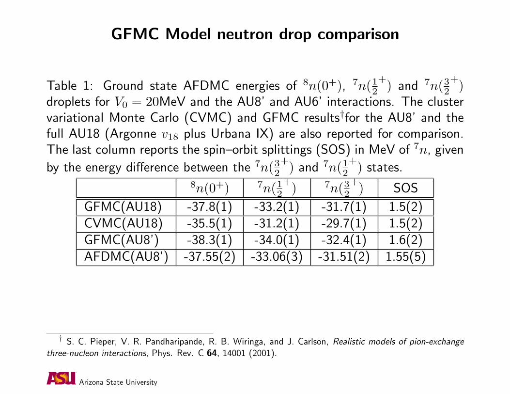
GFMC Model neutron drop comparison

Table 1: Ground state AFDMC energies of 8n(0+), 7n(12

+) and 7n(32

+)droplets for V0 = 20MeV and the AU8’ and AU6’ interactions. The clustervariational Monte Carlo (CVMC) and GFMC results†for the AU8’ and thefull AU18 (Argonne v18 plus Urbana IX) are also reported for comparison.The last column reports the spin–orbit splittings (SOS) in MeV of 7n, given

by the energy difference between the 7n(32

+) and 7n(12

+) states.8n(0+) 7n(1

2

+) 7n(32

+) SOS

GFMC(AU18) -37.8(1) -33.2(1) -31.7(1) 1.5(2)CVMC(AU18) -35.5(1) -31.2(1) -29.7(1) 1.5(2)GFMC(AU8’) -38.3(1) -34.0(1) -32.4(1) 1.6(2)AFDMC(AU8’) -37.55(2) -33.06(3) -31.51(2) 1.55(5)

† S. C. Pieper, V. R. Pandharipande, R. B. Wiringa, and J. Carlson, Realistic models of pion-exchangethree-nucleon interactions, Phys. Rev. C 64, 14001 (2001).


Neutron matter equation of state

0,2 0,4 0,6 0,8

ρ [fm-3]

0

100

200

300

E [

MeV

]

FP-AFDMC, AV8’Akmal, AV18FP-AFDMC, AV8’+UIXAkmal, AV18+UIX

Akmal refers to the FHNC calculation†

† A. Akmal, V.R. Pandharipande, and D.G. Ravenhall, Equation of state of nucleon matter and neutronstar structure, Phys. Rev. C 58 1804 (1998).


Low density neutron matter with Argonne v18

0 0,005 0,01 0,015 0,02 0,025 0,03 0,035

ρ [fm-3

]

0

1

2

3

4

5

6

7

E [

MeV

]

AV8’+UIXAV18+UIXFP

FP is the calculation of Friedman and Pandharipande (not v18, but the lowenergy channels are not very different).†

† B. Friedman and V.R. Pandharipande, Hot and cold, nuclear and neutron matter, Nucl. Phys. A361, 502 (1981).


Superfluid wave functions

We use a BCS form used here which is the standard BCS form projectedonto N particles.

For a bulk system of spin singlet pairs,

|BCS〉 =∏~k

[uk + vkc

+~k↑c+−~k↓

]|0〉

φ(~r1, s1;~r2, s2) ∝∑~k

vkuk

cos(~k · [~r1 − ~r2]

)[〈s1s2| ↑↓〉 − 〈s1s2| ↓↑〉]

In general

|BCS〉 =∏n

[un + vnc

+n c

+n′

]|0〉

φ(~r1, s1;~r2, s2) ∝∑n

vnun

[ψn(~r1, s1)ψn′(~r2, s2)− ψn(~r2, s2)ψn′(~r1, s1)]


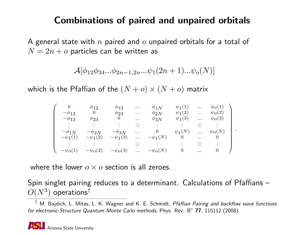
Combinations of paired and unpaired orbitals

A general state with n paired and o unpaired orbitals for a total ofN = 2n+ o particles can be written as

A[φ12φ34...φ2n−1,2n...ψ1(2n+ 1)...ψo(N)]

which is the Pfaffian of the (N + o)× (N + o) matrix

0BBBBBBBBBBBB@

0 φ12 φ13 ... φ1N ψ1(1) ... ψo(1)−φ12 0 φ23 ... φ2N ψ1(2) ... ψo(2)−φ13 φ23 0 ... φ3N ψ1(3) ... ψo(3)

......

............

......

.........

...−φ1N −φ2N −φ3N ... 0 ψ1(N) ... ψo(N)−ψ1(1) −ψ1(2) −ψ1(3) ... −ψ1(N) 0 ... 0

......

............

......

.........

...−ψo(1) −ψo(2) −ψo(3) ... −ψo(N) 0 ... 0

1CCCCCCCCCCCCA,

where the lower o× o section is all zeroes.

Spin singlet pairing reduces to a determinant. Calculations of Pfaffians –O(N3) operations†

† M. Bajdich, L. Mitas, L. K. Wagner and K. E. Schmidt, Pfaffian Pairing and backflow wave functionsfor electronic-Structure Quantum Monte Carlo methods, Phys. Rev. B” 77, 115112 (2008).


Central Spin Singlet Application

Dilute ≡ range R of the interaction � than interparticle spacing r0, or

kFR� 1, ρ = 34πr30

= k3F

3π2

If the scattering length a is large – short range interactions can stronglymodify the dilute gas properties, kF |a| � 1.

Low density neutron matter (in inner crust of neutron stars) R ∼ 2 fm,a = −18 fm.


Energy and even-odd energy gap for a = −∞ †

10 20 30 40A

0

10

20

E/E

FG

Pairing gap (∆) = 0.99(3) EFG

odd Aeven A

E = 0.44(1) A EFG

Energy as a function of particle number A.

Slater determinant nodes give an energy of E/A = 0.54EFG.

†J.Carlson, S-Y Chang, V.R. Pandharipande, and K.E. Schmidt, “Superfluid Fermi Gases with LargeScattering Length”, Phys. Rev. Lett. 91, 050401 (2003).


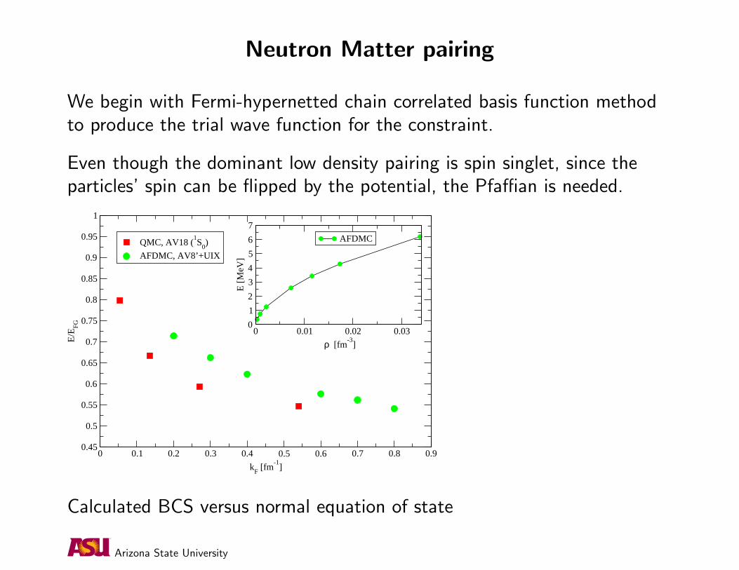
Neutron Matter pairing

We begin with Fermi-hypernetted chain correlated basis function methodto produce the trial wave function for the constraint.

Even though the dominant low density pairing is spin singlet, since theparticles’ spin can be flipped by the potential, the Pfaffian is needed.

0 0.1 0.2 0.3 0.4 0.5 0.6 0.7 0.8 0.9

kF [fm

-1]

0.45

0.5

0.55

0.6

0.65

0.7

0.75

0.8

0.85

0.9

0.95

1

E/E

FG

QMC, AV18 (1S

0)

AFDMC, AV8’+UIX

0 0.01 0.02 0.03

ρ [fm-3]

0

1

2

3

4

5

6

7

E [

MeV

]AFDMC

Calculated BCS versus normal equation of state


Neutron matter energy gaps

0 0.2 0.4 0.6 0.8 1

kF [fm

-1]

0

0.5

1

1.5

2

2.5

3∆

(MeV

)

BCSWambachChenSchulzeSchwenkCaoGezerlisFabrociniMargueronAFDMC

Calculated energies gap (AFDMC) compared to other calculations.


Spin Susceptibility

ρ/ρ0 Reid† Reid6‡ AU6’ AU8’ Reid60.75 0.45 0.53 0.40(1)1.25 0.42 0.50 0.37(1) 0.39(1) 0.36(1)2.0 0.39 0.47 0.33(1) 0.35(1)2.5 0.38 0.44 0.30(1)

Spin susceptibility ratio χ/χF of neutron matter. The AFDMC results forthe interactions AU6’, AU8’ and Reid6 are compared with those obtainedfrom the Landau parameters calculated from FHNC and CBF theories.The statistical error is given in parentheses.

† Brueckner calculations by S. O. Backmann and C. G. Kallman, Phys. Lett. B 43 (1973) 263.‡ CBF calculations by A. D. Jackson, E. Krotscheck, D. E. Meltzer and R. A. Smith, Nucl. Phys. A 386

(1992) 125.


Pion Condensate in neutron matter

• It has been conjectured that a “pion condensate” occurs in neutron stars

• This refers to a spin-density wave in neutron matter at high densities.

• The ~σ · ~∇π coupling to the pion field indicates that such a wave wouldbe accompanied by a pion field with a nonzero ground-state expectation– sort of a condensate.


Pion Condensate Results

PW = Plane wave model state

SD = Spin density wave model state


He Isotopes

4He

AFDMC v′6 -27.13(10) MeVHyperspherical v′6 -26.93(1) MeV†

GFMC v′6 -26.93(1) MeV [ -26.23(1) -0.7 MeV Coulomb ]‡

Expt -28.296 MeV

8He

AFDMC v′6 -23.6(5) MeV (Unstable to breakup into 4He+2n)GFMC v′6 -23.55(8) MeV [ -22.85(8) -0.7 MeV Coulomb ]Expt -31.408 MeV

† G. Orlandini, private communication‡ R.B. Wiringa and S.C. Pieper, Evolution of Nuclear Spectra with Nuclear Forces, Phys. Rev. Lett. 89,

182501 (2002).


Nuclear matter Energy, 28 particles, v′8 truncated to v6

0.5 1 1.5 2 2.5 3ρ /ρ0

-16

-14

-12

-10

-8

E [M

eV]

AFDMC fitAFDMCFHNC/SOCFHNC/SOC + elem.BHF

Dashed lines correspond to calculations performed with other methods†

(blue line with squares: FHNC/SOC; magenta with diamonds: BHF). Bluetriangles are FHNC/SOC results corrected with elementary diagrams.

† I. Bombaci, A. Fabrocini, A. Polls, I. Vidana, Spin-orbit tensor interactions in homogeneous matter ofnucleons: accurancy of modern many-body theories, Phys. Lett. B, 609, 232 (2005).


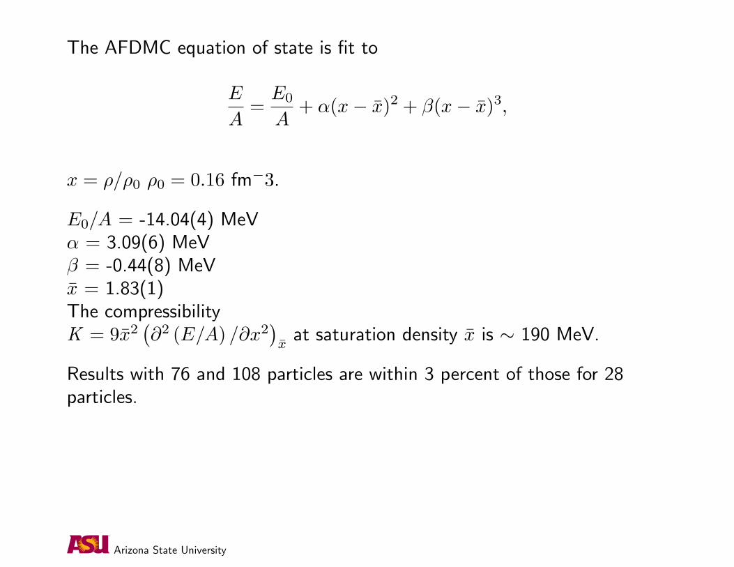
The AFDMC equation of state is fit to

E

A=E0

A+ α(x− x)2 + β(x− x)3,

x = ρ/ρ0 ρ0 = 0.16 fm−3.

E0/A = -14.04(4) MeVα = 3.09(6) MeVβ = -0.44(8) MeVx = 1.83(1)The compressibilityK = 9x2

(∂2 (E/A) /∂x2

)x

at saturation density x is ∼ 190 MeV.

Results with 76 and 108 particles are within 3 percent of those for 28particles.


Nuclear matter with Argonne v′6

Symmetric nuclear matter.

0.08 0.16 0.24 0.32 0.4 0.48

ρ [fm-3

]

-18

-16

-14

-12

-10

-8

-6

-4

E [

MeV

]

AFDMC, AV6’AFDMC, v

6’ (cut AV8’)

Comparison between Argonne v′8 truncated to v6 and Argonne v′6.


Asymmetric matter – some initial results

It’s easy to calculate with different numbers of neutrons and protons.

Removing size dependence is important.

0 0,05 0,1 0,15 0,2 0,25

ρ [fm-3

]

-15

-10

-5

0

5

10

15

E/A

[M

eV]

1.0, 66n0.95, 38n 1p0.9, 38n 2p0.867, 14n 1p0.78, 114n 14p0.75, 14n 2p0.65, 66n 14p0.46, 38n 14p0.0, 14n 14p

These are for Argonne v′6.


Conclusions and Future

• The auxiliary field Diffusion Monte Carlo calculations can give accurateresults for nuclei, neutron and nuclear matter.

• They have polynomial scaling with system size

• The three-body and spin-orbit potentials need to be included for theneutron-proton case.

• Asymmetric matter is straightforward, but size dependence needs to beaddressed.

• Physics of neutron rich nuclei can be studied – these are difficult toproduce in laboratories, but important for R-process reactions.

• Temperature > 0 is possible.


quantum monte carlo calculations of nuclear matter · quantum monte carlo calculations of nuclear...

Documents