October 28, 2004

Quantum mechanical reaction rate constants by vibrational

configuration interaction. Application to the OH + H2 Æ H2O + H

reaction as a function of temperature

Arindam Chakraborty and Donald G. Truhlar

Department of Chemistry and Supercomputing Institute, University of Minnesota,

Minneapolis, MN 55455-0431

Abstract. The thermal rate constant of the three-dimensional OH + H2 Ø H2O + H

reaction was computed using the flux autocorrelation function, with a time-independent

square-integrable basis set. Two modes that actively participate in bond making and bond

breaking were treated using two-dimensional distributed Gaussian functions, and the

remaining (nonreactive) modes were treated using harmonic oscillator functions. The

finite-basis eigenvalues and eigenvectors of the Hamiltonian were obtained by solving

the resulting generalized eigenvalue equation, and the flux autocorrelation function for a

dividing surface optimized in reduced-dimensionality calculations was represented in the

basis formed by the eigenvectors of the Hamiltonian. The rate constant was obtained by

integrating the flux autocorrelation function. The choice of the final time to which the

integration is carried is determined by a plateau criterion. The potential energy surface is

from Wu, Schatz, Lendvay, Fang, and Harding (WSLFH). We also studied the collinear

H + H2 reaction using the Liu-Siegbahn-Truhlar-Horowitz (LSTH) potential energy

surface. The calculated thermal rate constant results were compared with reported values

on the same surfaces. The success of these calculations demonstrates that time-

independent vibrational configuration can be a very convenient way to calculate

converged quantum mechanical rate constants, and it opens the door to calculating

converged rate constants for much larger reactions than have been treated up to now.

I. INTRODUCTION

The evaluation of the thermal reaction rate constant from the quantum

mechanical flux provides an efficient alternative to the computation of rate constants via

the scattering matrix. The quantum mechanical formulation of in terms of flux

autocorrelation functions

)(Tk

(k )T

)(f tC was presented by Yamamoto and Miller et al. (1−3), and

there have been several applications to calculate thermal rate constants for specific

systems. The flux operator can be used to compute the cumulative reaction probability

or the flux autocorrelation function, and either of these can be used to compute the

thermal rate constant. Various approaches (4−24) involving basis functions, path

integrals, and wave packet propagation methods have been used. Recently, Manthe et al.

have calculated the thermal rate constants for the CH

)(EN

4 + HØ CH3 + H2 and CH4 + O Ø

CH3 + OH reactions (19, 22) by calculating as a function of energy)(EN E using the

multi-configuration time-dependent Hartree (MCTDH) method. Earlier work on triatomic

reactions showed that accurate results can be obtained with an approach based on

diagonalizing the time-independent Hamiltonian (4, 8, 10). One advantage of this

formulation is that the variational principle is used to identify the relevant subspace of the

basis set. This approach is appealing in terms of its generality and straightforward

extension to larger systems, and it is extended to polyatomic reactions in the present

article.

In the present work, we have used flux autocorrelation functions to compute the

thermal rate constants of two benchmark reactions, collinear H + H2 Ø H2 + H (which is

used as a test of our new computer program) and full-dimensional OH + H2 Ø H2O + H.

Both of these reactions have been studied extensively in the past using various potential

energy surfaces (8, 11, 13, 16, 20, 22−37). In the present work, we have used a time-

independent square-integrable (L basis set to represent the Hamiltonian and the flux

operator, and we formulated the method in a way that should be applicable to general

polyatomic reactions. The basis functions are expressed in terms of mass-scaled normal

mode coordinates defined at the saddle point or at a variational transition state. We have

used two-dimensional distributed Gaussian functions to represent the two modes that

actively participate in the bond forming and bond breaking process. For the collinear H +

H

)2

2 Ø H2 + H reaction, there are only two modes, and both of these modes were treated

using two-dimensional distributed Gaussian functions. The use of distributed Gaussian

functions allows us to saturate the basis space in the strong interactions region, i.e., on

and around the transition state. A similar strategy was employed earlier for calculating

scattering matrices (38, 39).

The OH + H2 Ø H2O + H reaction has become a benchmark reaction for four-

atom systems. Recently, two new potential energy surfaces (33, 34) have been developed

for this reaction. We have used the Wu-Schatz-Lendvay-Fang-Harding (WSLFH)

potential energy WSLFH surface (33) for our work, and the resulting thermal rate

constants are compared with earlier wave packet calculations by Goldfield et al. (35).

There are six normal mode coordinates at the saddle point geometry, and the

Hamiltonian is represented as a function of the six mass-scaled normal mode coordinates.

Two stretching modes that represent the bond making and bond breaking process are

treated using two-dimensional distributed Gaussian functions, and the remaining four

modes are treated using harmonic oscillator basis functions. Six-dimensional basis

functions are formed by taking a direct product of the two-dimensional distributed

Gaussian functions with the harmonic oscillator functions, and the matrix elements of the

Hamiltonian operator are evaluated in this basis. Since the two-dimensional Gaussian

functions are not orthogonal to each other, the overlap matrix is computed, and the

generalized eigenvalue problem is solved to obtain the eigenvalues and eigenvectors. The

eigenvalues and eigenvectors are used to compute the flux autocorrelation function and

the thermal rate constant.

II. QUANTUM MECHANICAL THEORY

The thermal rate constant can be expressed in terms of the quantum mechanical flux

operator via the flux autocorrelation function (1−3). The derivation leading to this result for a

bimolecular reaction has been presented earlier (2), and so here we will simply summarize

the important relations. For further details, the reader is referred to refs. 3 and 8.

The expression for the symmetric flux operator is F

)],(,[ sHiF θh

= [1]

where h is Plank’s constant divided by ,2π H is the Hamiltonian operator, θ is the

Heaviside unit step function, s is the reaction coordinate, and 0=s defines a dividing

surface separating reactants from products. The flux autocorrelation function fC at time t

for a given temperature T is

},{Tr /22/f BB hh iHtTkHTkHiHt eFeeFeC −−−= [2]

where Tr{ } represents a quantum mechanical trace, and is Boltzmann’s constant.

The thermal rate constant is related to the flux autocorrelation function via

Bk

)(Tk

),(R

TSel TL

dk

Φ=σ

[3]

where σ is the symmetry number of the reaction,

is the electronic degeneracy of the

potential energy surface on which the reaction occurs (in the present case, is 2),

TSeld

TSeld RΦ is

the distinguishable-particle reactant partition function per unit volume, and is the

Laplace transform of the cumulative reaction probability given by

)(TL

),(B1 ENedEL TkE∫= −−h [4]

[5] .),(0

f∫=∞

dtTtC

One method of computing the flux correlation function is to evaluate the trace in Eq. 2, in the

basis formed from the eigenvectors of the Hamiltonian, and the resulting expression is

),cos(22/)(

fB t

EEFe ji

ijji

TkEE jih

C−

∑ ΨΨ=+− [6]

where and Ψ are the eigenvalues and eigenvectors of the Hamiltonian operator,

respectively. Inserting the expression of the flux operator from Eq. 1, we can rewrite Eq. 6 as

iE i

),cos()(1 222/)(2f

B tEE

EEe jiijji

ij

TkEE jihh

C−

−∑=+− θ [7]

where ijθ is the matrix element of the Heaviside step function in the basis formed from the

eigenvectors of the Hamiltonian operator.

In Eq. 3 the presence of σ indicates that we assume that and are calculated

without considering identical particle symmetry, and the presence of indicates that we

assume reaction occurs on a single Born-Oppenheimer potential energy surface of

L RΦ

TSeld

degeneracy . Carrying out the integral of Eq. 5 analytically for a finite upper limit t we

obtain

TSeld

t

(tI

iΨ

[8] ,)()(0

f∫ ′′≡≈t

tdtCtIL

where

).sin()(1 22/)( B tEE

EEeI TkEE

hh

γγγγγγ

γγθγγ ′

′′′

+− −−∑= ′

[9]

The upper limit should be chosen large enough that the correlation function has practically

decayed to zero, and the area under the C curve remains unchanged with time. Since total

angular momentum is a good quantum number, we calculate the contributions of each

value to or separately. We therefore write

f

J J

L )

[10] .)()12(∑ +=J

J TLJL

In order to evaluate the rate constant using Eq. 9 we need the eigenvectors and

eigenvectors of the Hamiltonian operator. We expand the eigenvectors in a nonorthogonal

basis as:

iE

,∑ Φ=Ψk

kkii c [11]

where the overlap matrix S is

.kkkkS ′′ ΦΦ= [12]

The eigenvalues were obtained by solving the generalized eigenvalue equation

,iii E ScHc = [13]

where is the Hamiltonian matrix in the nonorthogonal basis, and c is the eigenvector

with elements c .

H i

ki

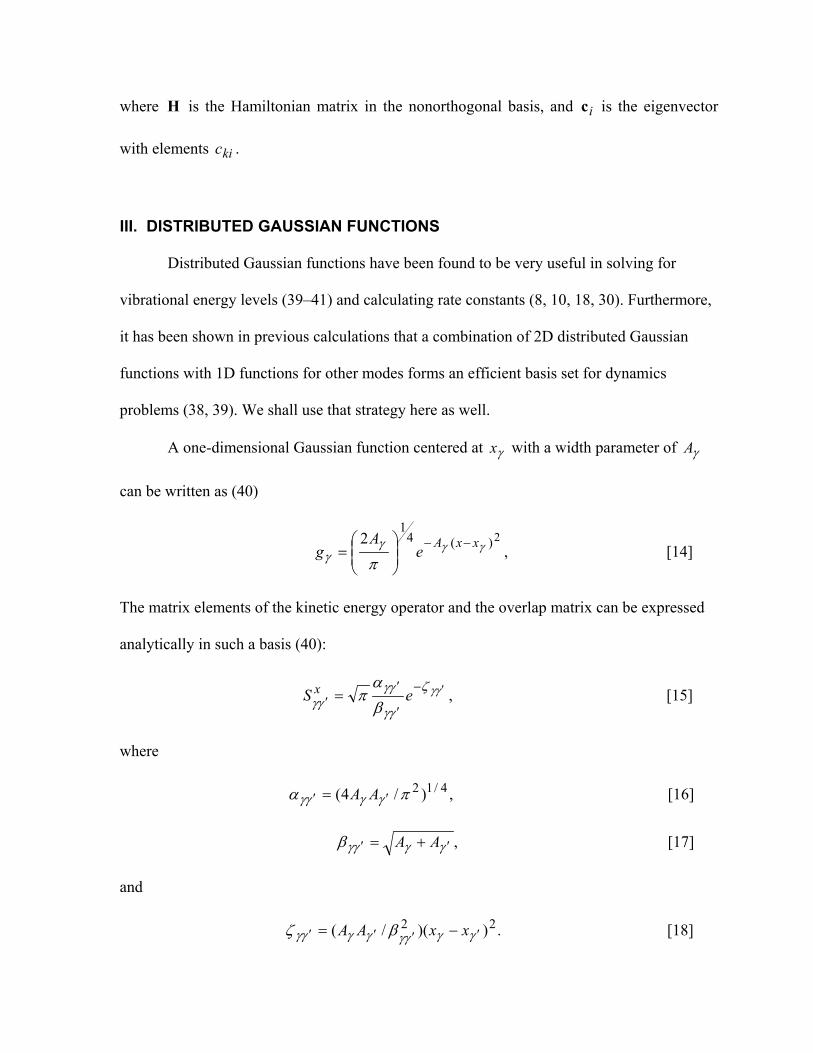
III. DISTRIBUTED GAUSSIAN FUNCTIONS

Distributed Gaussian functions have been found to be very useful in solving for

vibrational energy levels (39–41) and calculating rate constants (8, 10, 18, 30). Furthermore,

it has been shown in previous calculations that a combination of 2D distributed Gaussian

functions with 1D functions for other modes forms an efficient basis set for dynamics

problems (38, 39). We shall use that strategy here as well.

A one-dimensional Gaussian function centered at with a width parameter of

can be written as (40)

γx γA

,2 2)(4

1γγ

πγ

γxxAe

Ag −−

= [14]

The matrix elements of the kinetic energy operator and the overlap matrix can be expressed

analytically in such a basis (40):

,γγζ

γγ

γγγγ β

απ ′−

′

′′ = eS x [15]

where

[16] ,)/4( 4/12πα γγγγ ′′ = AA

,γγγγβ ′′ += AA [17]

and

[18] .))(/( 22γγγγγγγγ βζ ′′′′ −= xxAA

In these equations, the elements of the overlap matrix are represented by where the

superscript

xS γγ ′

x is used to denote that the Gaussians are functions of x . Although this notation

is not important for 1D Gaussian, it is useful for describing matrix elements of 2D Gaussian

functions, which are described next.

One can also construct a 2D Gaussian in the xy plane by taking a direct product of

Gaussian functions along the x and axes: y

).,;(),;( γγγγγγγχ yAygxAxg ′= [19]

Although one can optimize grids of 2D Gaussian functions (6, 38, 39, 42, 43), in the present

work we start with direct products and use an energy cutoff (described below) to optimize the

final selection of basis functions. The overlap and the kinetic energy integrals for the 2D

Gaussian can be written in term of those for 1D Gaussian functions:

[20] ,yx SSS γγγγγγ ′′′ =

A set of distributed 2D Gaussian functions of the form of Eq. 19 has parameters. In

order to reduce the number of parameters we use a single width parameter (

N N4

)AAA ≡′= γγ

for all Gaussian functions. The value of is chosen such that the overlap between any two

2D Gaussians never exceeds a prespecified value. The details for the overlap cutoff will be

discussed in Sec. V.

γA

IV. COLLINEAR H + H2 SYSTEM

The collinear H + H2 reaction has been studied extensively (6, 25, 28) and here it

is used to validate the method. The details are given in Appendix A of supporting

information. The results agree with those calculated by scattering theory (28) within 1%.

V. OH + H2 CALCULATION

The three hydrogen atoms in the OH + H2 system were labeled as

HAO + HBHCØ HAOHB + HC. [21]

The OH + H2 system has six vibrational degrees of freedom. Normal mode

analysis was performed at the saddle point geometry, and the resulting frequencies are

3675, 2439, 1191, 690, and 573 cm-1 for modes 1-5, respectively, and 1210i cm-1 for

mode 6. The modes Q , , Q , and Q modes represent the spectator O-H stretch, the

out-of-plane bend, the in-plane bend, and the torsion, respectively. The two stretch modes

that actively participate in the bond making and bond breaking process are Q and .

All Q are zero at the saddle point. The two reactive modes were

represented using 2D distributed Gaussian functions. The remaining four spectator modes

were represented by harmonic oscillator (HO) functions. The 6D basis was formed by

taking a direct product between 2D distributed Gaussian functions and the HO functions.

Earlier work (31) has shown that the contribution of the vibrational angular momentum

term is very small for this system and can be dropped from the expression of the

Hamiltonian. Therefore the Hamiltonian in mass-scaled (27) normal coordinates is

1

)6,

3Q 4 5

2 6Q

,2,1( K=mm

),,,(2 61

6

1 2

22QQV

QH

i iK

h+∑

∂

∂−=

=µ [22]

whereµ is the scaling mass. In the present calculations the value ofµ was set at 1 amu.

The matrix elements of the Hamiltonian operator were evaluated using six-dimensional

basis functions, and the resulting generalized eigenvalue equation was solved.

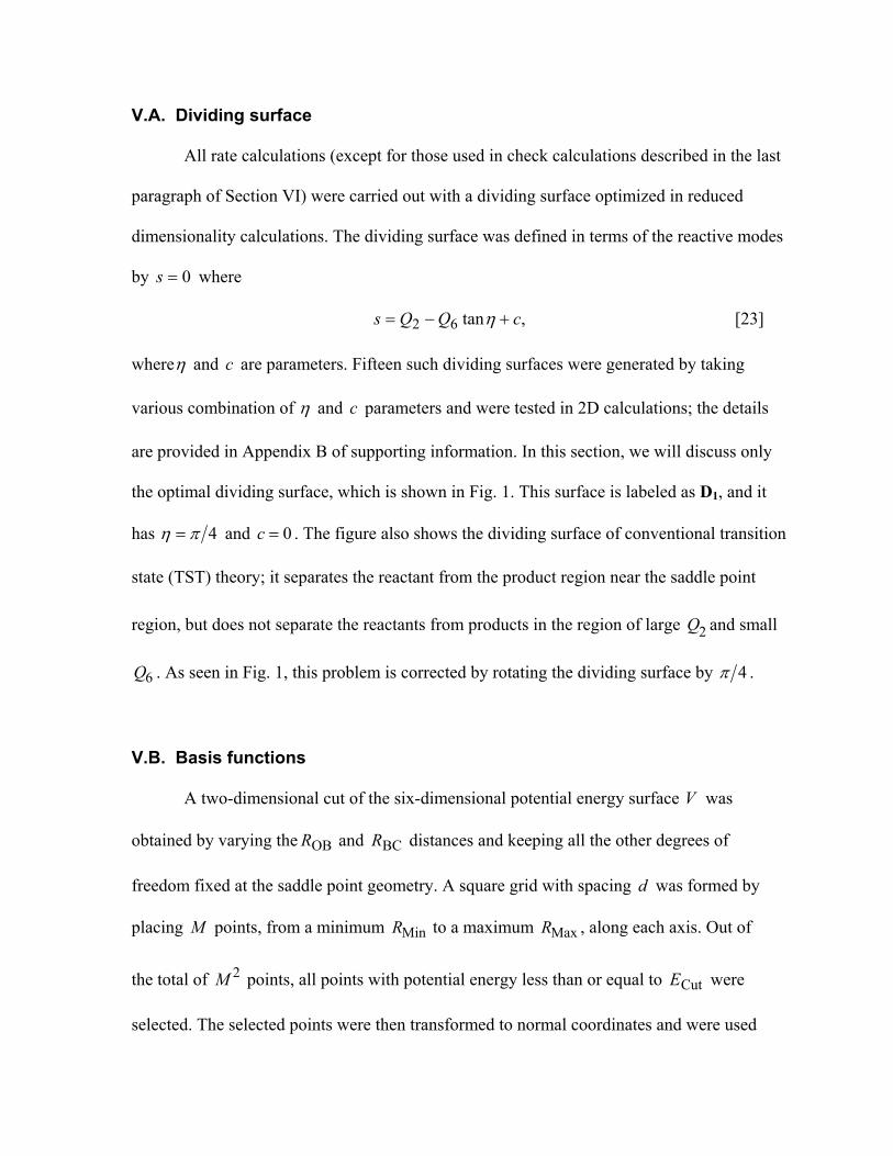
V.A. Dividing surface

All rate calculations (except for those used in check calculations described in the last

paragraph of Section VI) were carried out with a dividing surface optimized in reduced

dimensionality calculations. The dividing surface was defined in terms of the reactive modes

by where 0=s

,tan62 cQQs +−= η [23]

whereη and are parameters. Fifteen such dividing surfaces were generated by taking

various combination of

c

η and parameters and were tested in 2D calculations; the details

are provided in Appendix B of supporting information. In this section, we will discuss only

the optimal dividing surface, which is shown in Fig. 1. This surface is labeled as D

c

1, and it

has 4πη = and c . The figure also shows the dividing surface of conventional transition

state (TST) theory; it separates the reactant from the product region near the saddle point

region, but does not separate the reactants from products in the region of large and small

. As seen in Fig. 1, this problem is corrected by rotating the dividing surface by

0=

2Q

6Q 4π .

V.B. Basis functions

A two-dimensional cut of the six-dimensional potential energy surface V was

obtained by varying the and distances and keeping all the other degrees of

freedom fixed at the saddle point geometry. A square grid with spacing d was formed by

placing

OBR BCR

M points, from a minimum to a maximum , along each axis. Out of

the total of

MinR MaxR

2M points, all points with potential energy less than or equal to were

selected. The selected points were then transformed to normal coordinates and were used

CutE

as centers for two-dimensional distributed Gaussian functions with 6Qx = and

The number of two-dimensional Gaussian functions formed is called . All

Gaussian functions were assigned the same width parameter such that the maximum

overlap between any two Gaussian functions is less than or equal to .

.2Qy =

gNgN

MaxS

62Q

A

,

The number of basis functions used for the six-dimensional calculations is directly

proportional to the number of 2D Gaussian functions. It is desirable to have a small value

of so that the number of basis functions for the 6D calculations is affordable. We

therefore carried out reduced-dimensional calculations whose purpose was to optimize the

2D distributed Gaussian functions.

N

gN

gN

The reduced-dimensional calculations were performed in the Q subspace, with

the other vibrational degrees of freedom frozen at their saddle point values. The calculations

were repeated with various sets of 2D Gaussian functions, and the parameters were varied to

find small basis sets that yield converged results in 2D. Table 1 lists parameters for two

different sets of 2D Gaussian basis functions, labeled as G1 and G2, that yield converged flux

autocorrelation functions in 2D for the temperature range of 300–1000 K. The G2 set has a

larger value for the cutoff energy and a smaller value of grid spacing d and it contains

more basis functions than the G

CutE ,

1 set. The centers of the 243 distributed Gaussian functions in

set G1 are shown in Fig. 1. This set was selected for use in 6D calculations.

The basis functions are functions of six normal coordinates and are given by

),( HO62 kkk QQ Φ=Φ χ [24]

where

Φ [25] ),()()()( 5431HO

5431 QQQQ kkkk nnnnk ϕϕϕϕ=

and mknϕ is an HO function, with orders .,1,0 K=mkn Note that Eq. 24 does not include

rotation. One could carry out calculations for nonzero total angular momentum by

multiplying Eq. 24 by a rotational function (44-47). In the present article we use basis

functions only for Since the

J

.0=J 0=J rotational eigenfunction is a constant, including

rotation in Eq. 24 only affects the normalization. Note that HOkΦ is an eigenfunction of the

four-dimensional HO Hamiltonian defined at the saddle point geometry, with eigenvalue

,~55443311

HO ωωωω hhhh kkkkk nnnnE +++= [26]

where mω is the frequency of mode at the saddle point. Note that the zero point energy of

the four-dimensional HO is included in the zero of energy. The 6D basis functions were

formed by taking a direct product between 4D harmonic oscillator functions and

2D Gaussian functions, resulting in

,m

N

HON

HOg N

gN

N= six-dimensional basis functions. The

procedure used to select the HO functions is discussed in Sec. VI.

V.C. Thermal rate constant calculations

The matrix elements needed in Eqs. 9 and 13 were computed by standard methods as

explained in Appendix C of supporting information. The eigenvalues and eigenvectors of the

Hamiltonian were obtained from Eq. 13, and the 0=J contribution to the Laplace

transform was obtained from Eqs. 8 and 9. The integral depends on the upper limit of the

integration, and we must choose the upper limit large enough that the results are converged

(3, 8). However, due to the finite size of the basis, the integral does not really converge, but

)(0 TLJ =

t

only reaches a plateau. Figure 2 shows )(f tC and the 300 K integral for the time range 0 to

60 fs. We see that in the 0–20 fs and 40–60 fs regions the value fluctuates with t , but it is

very stable in the time range of 30–40 fs. One can use this plateau value of to compute

thermal rate constants. Factors that affect the range of time over which is stable at its

plateau value include the number of basis functions used for the calculation, the locations of

the basis functions, and the position of the dividing surface. The type of basis functions is

also an important factor; for example, it was shown by ref. 5 that 1D distributed Gaussian

functions and sine functions are more efficient basis functions than harmonic oscillator

functions for evaluating

)(tI

)(tI

)(tI

fC for a 1D Eckart potential.

JL

)TSTS

3B

C

T

/TS hc

)(TL

TS

/TS

The value of the upper limit of time integration was determined in the present work

by finding the widest time interval over which is constant to within 1%. The center of

this interval is called

)(tI

ft and the width is called t∆ . (Details of the algorithm for finding ft

are in Appendix D of supporting information.) We take )( ftI as . 0=

Rather than compute by the exact relation of Eq. 10, we use the separable-rotation

approximation (48), which yields

L

,( 0TS

== JLBA

kπ [27]

where are the rotational constants of the transition state evaluated at the

saddle point geometry. The values of and C were 18.2 cm

TSTS and , , CBA

,A ,/ TS hcB hc -1, 2.81

cm-1, and 2.44 cm-1, respectively. These values are identical to the values used by Goldfield

et al. (35). It is known form previous work (20, 35) that the separable-rotation approximation

overestimates the rate constant by about 40% for this reaction.

Finally, we consider three other factors in Eq. 3. The symmetry number σ is 2, the

electronic degeneracy d is 2, and TSel

[28] ,Rrotvib

RelRel

R−Φ=Φ Qg

whereΦ is the relative translational partition function per unit volume, and is the

reactant electronic partition function given by

Rel Relg

[29] ,22 B/Rel

Tkhceg ∆−+=

where is the spin-orbit splitting of the OH radical and equals140 (49). Q is

the product of two diatomic vibrational-rotational partition functions Q computed

without considering identical-particle symmetry or nuclear spin (those effects are in

∆ -1cm

diatvib

Rrotvib−

rot−

σ ). For

consistency with Eq. 27, these are computed from the diatomic rotational constant and

vibrational energy levels and diatomic rotational constant diatB by

,diatvibdiat

Bdiatrotvib Q

B

Tk=−Q [30]

with Q evaluated from the accurate diatomic energy levels for the given potential energy

surface.

diatvib

VI. RESULTS FOR OH + H2 Æ H2O + H

This section discusses the convergence with respect to the HO basis functions in

the nonreactive degrees of freedom and compares the results to previous calculations.

The parameters for the basis functions used for the computation of thermal rate

constant are shown in Table 2. Four-dimensional spaces of basis sets B1-B3 were

obtained by a two-step procedure. In the first step, a cutoff parameter HOMax

~E was defined,

and all HOkΦ with HO

MaxHO ~~ EEk ≤ were selected for the next step. Among

these HOkΦ selected, only functions with three of the four , with mn ,5and,4,3,1=m

equal to zero were selected. As an example, consider a basis set formed using

.cm5000~ 1

5000

HOMax

−E = There are 91 four-dimensional HO functions with excitations

energies less that or equal to Out of these 91 functions, there are only 21

functions with three or more

.cm 1−

0=mn

max5n

0,( max1 kn +

. Basis sets B4-B8 are variations on basis B1. First,

the maximum number of quanta in each of the four modes for the B1 set was labeled as

, n , n , and , respectively. For Bmax1n max

4max3 4 three new harmonics oscillator

functions of the form with )0,0, 3,,1 K=k were formed and were

combined with the 18 existing harmonic oscillator function in the B1 set to give a set of

21 harmonic oscillator functions. Similar procedure was carried out with n , n ,

and to yield B

max max43

max5n 5-B7. Note that B4-B7 all contain 5103 6D functions, but they have

different distributions of quanta in the four nonreactive modes. Table 3 shows good

convergence of the thermal rate constants computed using B1-B7 sets.

Convergence of the B1 set was also tested by using two-mode excited HO

functions in the basis set. There are five possible combinations for exciting any two

modes at the same time: , , , ,

, and ( . The three lowest energy states of the form

were combined with the 18 harmonic oscillator functions from the B

)0,0,,( 31 nn

), 54 nn

)0,,0,( 41 nn ),0,0,( 51 nn )0,,,0( 43 nn

),0,,0( 53 nn

)0,0,,( 31 nn

,0,0

1 set to

obtain a new set of 21 harmonic oscillator functions. The direct product between these 21

harmonic oscillator functions and 243 distributed Gaussian functions was formed and the

resulting set of 5103 functions was labeled as B8. Similar calculations were also

performed for the remaining four combinations, and the results for B9-B13 were found to

agree well with those for B1-B7. The largest deviation for any of the results with bases

B4–B13 from those obtained with our largest basis, B3 is 1%.

The flux autocorrelation functions for the B1 set at 300 K and 1000 K are shown

in Figs. 2 and 3. We see that in both cases fC rapidly approaches a small constant value

and maintains that value, before showing the expected oscillations at large time. The

plots for the corresponding are also shown. These plots exhibit the broad stable

region that is important for accurate determination of rate constants.

)(tI

We have also calculated rate constants at 300 K and 500 K using dividing

surfaces based on variational transition state theory (VTST). The results agree with those

presented here within 1% in both cases. Figure 4 shows plots of the flux autocorrelation

function obtained using the dividing surface at the saddle point and the variational

dividing surface at 300 K. This provides a numerical verification of the fact that the

results are independent of the location of the dividing surface. Details of these check

calculations are provided in Appendix E of supporting information.

Not only are the results well converged, but they agree well with the wave packet

results of ref. 35. Over the temperature range 300–1000 K, the largest deviation and the

mean unsigned deviation for any of the B1-B13 basis sets from the results obtained in ref.

35 was 7% and 2%, respectively. (In comparing to ref. 35, we compare to their

separable-rotation results because the emphasis in the present paper is on calculation of

the Laplace transform, not on improving on separable-rotation approximation.)

VII. CONCLUSIONS

The thermal rate constant was computed for a full-dimensional four-body reaction

using time-independent square-integrable basis functions, and the Laplace transform was

found to be well converged and in good agreement with previous calculations based on time-

dependent wave packets. This is the first time that rate constants for a system with more than

three atoms have been calculated by any method that uses time-independent basis functions.

It was shown that an efficient basis set can be formed by using Gaussian basis functions for

the two active stretch modes and HO functions for the remaining modes. We found that the

number of HO functions needed in the nonreactive degrees of freedom to get converged

results is very small as compared to the number of two-dimensional distributed Gaussian

functions in the bond forming and bond breaking modes.

Although much of the effort in quantum dynamics is currently focused on wave

packet methods, the success of the present calculation opens the door to treating general

multi-dimensional reactions by convenient time-independent basis set methods, and we

anticipate that further reduction in the computational cost can be achieved by combining the

present methods with new schemes (42, 43) for reducing the size of Gaussian basis sets for

nuclear motion and with hierarchical representations of the potential (44-47). This

comparison of time-independent to time-dependent approaches bears elaboration. It is a

general question of working in the time domain or the energy domain, which are

complementary in a Fourier sense. In the early days of quantum mechanical collision theory,

time-independent methods, especially the close coupling method, received almost all of the

attention and effort (50–52). Later, attention turned more to time-dependent quantum

dynamics (53, 54), which is now considered by most workers to be the method of choice for

accurate polyatomic dynamics (55, 56). Time-dependent quantum mechanics is especially

efficient for generating results at a series of total energies, as required for thermally averaged

rate constants, because a single wave packet carries information about a wide range of

energies (54). The present application though shows that time-independent quantum

mechanics can also be used for accurate polyatomic reaction dynamics. It is particularly

important to point out that the method used here is not special to four-body reactions, and in

fact it is based on straightforward use of vibrational configuration interaction. Thus, by

taking advantage of recent advances in vibrational configuration interaction calculations

(45-47) and the fast convergence of the calculations with respect to completing the basis in

nonreactive degrees of freedom, it should be possible to extend the method used here to

much larger systems. In this regard, we note that use of the flux autocorrelation method

(1-3) is a general method for taking advantage of the fact that reaction rates are often

dominated by short-time dynamics in a localized region around a transition state. This makes

time-dependent methods like the time-dependent Hartree method (18-20, 22, 55-57) more

affordable because the wave packet needs to be represented over only a short period of time,

and time-independent methods like vibrational configuration also benefit greatly by the need

to represent the wave function over only a localized region of space. We anticipate that

vibrational-rotational configuration interaction calculations will provide a powerful general

tool for calculating flux autocorrelation functions for many other polyatomic reactions.

VIII. ACKNOWLEDGMENTS

The authors are grateful to Stephen Gray for sending the reaction rate constants of

ref. 35 in tabular form. This work was supported in part by the National Science

Foundation, through grant no. CHE-0092019.

References

1. Yamamoto, T. (1960) J. Chem. Phys. 33, 281–289.

2. Miller, W. H. (1974) J. Chem. Phys. 74, 1823–1834.

3. Miller, W. H., Schwartz, S. D. & Tromp, J. W. (1983) J. Chem. Phys. 79, 4889–4898.

4. Tromp, J. W. & Miller, W. H. (1987) Faraday Discuss. Chem. Soc. 84, 441–453.

5. Wyatt, R. E. (1985) Chem. Phys. Lett. 121, 301–306.

6. Park, T. J. & Light, J. C. (1988) J. Chem. Phys. 88, 4897–4912.

7. Park, T. J. & Light, J. C. (1989) J. Chem. Phys. 91, 974–988.

8. Day, P. N. & Truhlar, D. G. (1991) J. Chem. Phys. 94, 2045–2056.

9. Seideman, T. & Miller, W. H. (1991) J. Chem. Phys. 95, 1768–1780.

10. Day, P. N. & Truhlar, D. G. (1991) J. Chem. Phys. 95, 5097–5112.

11. Park, T. J. & Light, J. C. (1992) J. Chem. Phys. 96, 8853–8862.

12. Lefebvre, R., Ryaboy, V. & Moiseyev, M. (1993) J. Chem. Phys. 98, 8601–8605.

13. Manthe, U. & Miller, W. H. (1993) J. Chem. Phys. 99, 3411–3419.

14. Moiseyev, M. (1995) J. Chem. Phys. 103, 2970–2973.

15. Thompson, W. H. & Miller, W. H. (1997) J. Chem. Phys. 106, 142–150.

16. Zhang, D. H. & Light, J. C. (1997) J. Chem. Phys. 106, 551–563.

17. Wang, H., Thompson, W. H. & Miller, W. H. (1997) J. Chem. Phys. 107, 7194–7201.

18. Matzkies, F. & Manthe, U. (2000) J. Chem. Phys. 112, 130–136.

19. Huarte-Larrañaga, F. & Manthe, U. (2000) J. Chem. Phys. 113, 5115–5118.

20. Manthe, U. & Matzkies. F. (2000) J. Chem. Phys. 113, 5725–5731.

21. Tolstikhin, O. I., Ostrovsky, V. N. & Nakamura, H. (2001) Phys. Rev. A 63,

042707/1–18.

22. Huarte-Larrañaga, F. & Manthe. U. (2002) J. Chem. Phys. 117, 4635–4638.

23. Defazio, P. & Gray, S. K. (2003) J. Phys. Chem. A 107, 7132–7137.

24. Medvedev, D. M. & Gray, S. K. (2004) J. Chem. Phys. 120, 9060–9070.

25. Truhlar, D. G. & Wyatt, R .E. (1976) in Annual Review of Physical Chemistry, Vol.

27, ed. Rabinovitch, B. S. (Annual Reviews, Inc., Palo Alto), pp. 1–43.

26. Truhlar, D. G. & Horowitz, C. J. (1978) J. Chem. Phys. 68, 2466–2476.

27. Isaacson, A. D. & Truhlar, D. G. (1982) J. Chem. Phys. 76, 1380–1391.

28. Bondi, D. K., Clary, D. C., Connor, J. N. L., Garrett, B. C. & Truhlar, D. G. (1982) J.

Chem. Phys. 76, 4986–4995.

29. Manthe, U., Seideman, T. & Miller, W. H. (1993) J. Chem. Phys. 99, 10078–10081.

30. Mielke, S. L., Lynch. G. C., Truhlar, D. G. & Schwenke, D. W. (1994) J. Chem.

Phys. 98, 8000–8008.

31. Manthe, U., Seideman, T. & W. H. Miller (1994) J. Chem. Phys. 101, 4759–4768.

32. Chatfield, D. C., Mielke, S. L., Allison, T. C. & Truhlar, D. G. (2000) J. Chem. Phys.

112, 8387–8408.

33. Wu, G.-S., Schatz, G. C., Lendvay, G., Fang, D.-C & Harding, L. B. (2000) J. Chem.

Phys. 113, 3150–3161.

34. Yang, M., Zhang, D. H., Collins, M.A., & Lee. S.-Y. (2001) J. Chem. Phys. 115,

174–178.

35. Goldfield, E. M. & Gray, S. K. (2002) J. Chem. Phys. 117, 1604–1613.

36. Mielke, S. L., Peterson. K. A., Schwenke, D. W., Garrett, B. C., Truhlar, D. G.,

Michael, J. V., Su, M.-C. & Sitherland, J. W. (2003) Phys. Rev. Lett. 91, 063201/1–4.

37. Zhang, J. Z. H., Li, Y. M., Wang, L. & Xiang, Y. (2004) in Modern Trends in

Chemical Reaction Dynamics, eds. Yang, X. & Liu, K. (World Scientific, Singapore),

pp. 209–248.

38. Tawa, G. J., Mielke, S. L., Truhlar, D. G., & Schwenke, D. W. (1994) J. Chem. Phys.

100, 5751–5777.

39. Hack, M. D., Jasper, A. W., Volobuev, Y. L., Schwenke, D. W. & Truhlar, D. G. J.

Phys. Chem. A (1999) 103, 6309–6326.

40. Hamilton, I. P. & Light, J. C. (1986) J. Chem. Phys. 84, 306–317.

41. Day, P. N. & Truhlar, D. G. (1991) J. Chem. Phys. 95, 6615–6621.

42. Poirer, B. & Light, J. C. (2000) J. Chem. Phys. 113, 211–217.

43. Garashchuk, S. & Light, J. C. (2001) J. Chem. Phys. 114, 3929–3939.

44. Carter, S., Culik, S. J. & Bowman. J. M. (1997) J. Chem. Phys. 107, 10458–10469.

45. Carter, S. & Bowman, J. M. (1998) J. Chem. Phys. 108, 4397–4404.

46. Carter, S., Bowman, J. M. & Handy, N. C. (1998) Theor. Chem. Acc. 100, 191–198.

47. Chakraborty, A., Truhlar, D. G., Bowman, J. M. & Carter, S. C. (2004) J. Chem.

Phys. 121, 2071–2084.

48. Mielke, S. L., Lynch. G. C., Truhlar, D. G. & Schwenke, D. W. (1993) Chem. Phys.

Lett. 216, 441–446.

49. Herzberg, G. (1950) Molecular Spectra and Molecular Structure. I. Spectra of

Diatomic Molecules (Van Nostrand, Princeton).

50. Bernstein, R. B., ed. (1979) Atom-Molecule Collision Theory (Plenum, New York).

51. Clary, D. C., ed. (1986) The Theory of Chemical Reaction Dynamics (Reidel,

Dordrecht, Holland).

52. Truhlar, D. G. (1994) Computer Phys. Commun. 84, 79-90.

53. Kulander, K. C., ed. (1991) Time-Dependent Methods for Quantum Dynamics

[special issue of Computer Phys. Commun. 63, 1-584] (Elsevier, Amsterdam).

54. Wyatt, R. E. & Zhang, J. Z. H., eds. (1996) Dynamics of Molecules and Chemical

Reactions (Dekker, New York).

55. Beck, M. H., Jäckle, A., Worth, G. A. & Meyer, H.-D. (2000) Physics Reports 324,

1–105.

56. Meyer, H.-D. & Worth, G. A. (2003) Theor. Chem. Acc. 109, 251–267.

57. Meyer, H.-D., Manthe, U. & Cederbaum, L. S. (1990) Chem. Phys. Lett. 165, 73–78.