quantum mechanical path integral · 14 quantum mechanical path integral 2.3 how to evaluate the...
TRANSCRIPT
Chapter 2
Quantum Mechanical Path Integral
2.1 The Double Slit Experiment
Will be supplied at later date
2.2 Axioms for Quantum Mechanical Description of Single Parti-cle
Let us consider a particle which is described by a Lagrangian L(~r, ~r, t). We provide now a set offormal rules which state how the probability to observe such a particle at some space–time point~r, t is described in Quantum Mechanics.
1. The particle is described by a wave function ψ(~r, t)
ψ : R3 ⊗ R → C. (2.1)
2. The probability that the particle is detected at space–time point ~r, t is
|ψ(~r, t)|2 = ψ(~r, t)ψ(~r, t) (2.2)
where z is the conjugate complex of z.
3. The probability to detect the particle with a detector of sensitivity f(~r) is∫Ωd3r f(~r) |ψ(~r, t)|2 (2.3)
where Ω is the space volume in which the particle can exist. At present one may think off(~r) as a sum over δ–functions which represent a multi–slit screen, placed into the space atsome particular time and with a detector behind each slit.
4. The wave function ψ(~r, t) is normalized∫Ωd3r |ψ(~r, t)|2 = 1 ∀t, t ∈ [t0, t1] , (2.4)
a condition which enforces that the probability of finding the particle somewhere in Ω at anyparticular time t in an interval [t0, t1] in which the particle is known to exist, is unity.
11
12 Quantum Mechanical Path Integral
5. The time evolution of ψ(~r, t) is described by a linear map of the type
ψ(~r, t) =∫
Ωd3r′ φ(~r, t|~r′, t′)ψ(~r′, t′) t > t′, t, t′ ∈ [t0, t1] (2.5)
6. Since (2.4) holds for all times, the propagator is unitary, i.e., (t > t′, t, t′ ∈ [t0, t1])∫Ω d
3r |ψ(~r, t)|2 =∫Ω d
3r∫
Ω d3r′∫
Ω d3r′′ φ(~r, t|~r′, t′) φ(~r, t|~r′′, t′) ψ(~r′, t′) ψ(~r′′, t′)=∫
Ω d3r |ψ(~r, t′)|2 = 1 . (2.6)
This must hold for any ψ(~r′, t′) which requires∫Ωd3r′ φ(~r, t|~r′, t′)φ(~r, t|~r′′, t′) = δ(~r′ − ~r′′) (2.7)
7. The following so-called completeness relationship holds for the propagator (t > t′ t, t′ ∈[t0, t1]) ∫
Ωd3r φ(~r, t|~r′, t′) φ(~r′, t′|~r0, t0) = φ(~r, t|~r0, t0) (2.8)
This relationship has the following interpretation: Assume that at time t0 a particle is gen-erated by a source at one point ~r0 in space, i.e., ψ(~r0, t0) = δ(~r − ~r0). The state of a systemat time t, described by ψ(~r, t), requires then according to (2.8) a knowledge of the state at allspace points ~r′ ∈ Ω at some intermediate time t′. This is different from the classical situationwhere the particle follows a discrete path and, hence, at any intermediate time the particleneeds only be known at one space point, namely the point on the classical path at time t′.
8. The generalization of the completeness property to N − 1 intermediate points t > tN−1 >tN−2 > . . . > t1 > t0 is
φ(~r, t|~r0, t0) =∫
Ω d3rN−1
∫Ω d
3rN−2 · · ·∫
Ω d3r1
φ(~r,t|~rN−1, tN−1) φ(~rN−1, tN−1|~rN−2, tN−2) · · ·φ(~r1, t1|~r0, t0) . (2.9)
Employing a continuum of intermediate times t′ ∈ [t0, t1] yields an expression of the form
φ(~r, t|~r0, t0) =∫∫ ~r(tN )=~rN
~r(t0)=~r0
d[~r(t)] Φ[~r(t)] . (2.10)
We have introduced here a new symbol, the path integral∫∫ ~r(tN )=~rN
~r(t0)=~r0
d[~r(t)] · · · (2.11)
which denotes an integral over all paths ~r(t) with end points ~r(t0) = ~r0 and ~r(tN ) = ~rN .This symbol will be defined further below. The definition will actually assume an infinitenumber of intermediate times and express the path integral through integrals of the type(2.9) for N → ∞.

2.2: Axioms 13
9. The functional Φ[~r(t)] in (2.11) is
Φ[~r(t)] = expi
~
S[~r(t)]
(2.12)
where S[~r(t)] is the classical action integral
S[~r(t)] =∫ tN
t0
dtL(~r, ~r, t) (2.13)
and
~ = 1.0545 · 10−27 erg s . (2.14)
In (2.13) L(~r, ~r, t) is the Lagrangian of the classical particle. However, in complete distinctionfrom Classical Mechanics, expressions (2.12, 2.13) are built on action integrals for all possiblepaths, not only for the classical path. Situations which are well described classically will bedistinguished through the property that the classical path gives the dominant, actually oftenessentially exclusive, contribution to the path integral (2.12, 2.13). However, for microscopicparticles like the electron this is by no means the case, i.e., for the electron many pathscontribute and the action integrals for non-classical paths need to be known.
The constant ~ given in (2.14) has the same dimension as the action integral S[~r(t)]. Its valueis extremely small in comparision with typical values for action integrals of macroscopic particles.However, it is comparable to action integrals as they arise for microscopic particles under typicalcircumstances. To show this we consider the value of the action integral for a particle of massm = 1 g moving over a distance of 1 cm/s in a time period of 1 s. The value of S[~r(t)] is then
Scl =12mv2 t =
12
erg s . (2.15)
The exponent of (2.12) is then Scl/~ ≈ 0.5 · 1027, i.e., a very large number. Since this number ismultiplied by ‘i’, the exponent is a very large imaginary number. Any variations of Scl would thenlead to strong oscillations of the contributions exp( i
~S) to the path integral and one can expect
destructive interference betwen these contributions. Only for paths close to the classical path issuch interference ruled out, namely due to the property of the classical path to be an extremal ofthe action integral. This implies that small variations of the path near the classical path alter thevalue of the action integral by very little, such that destructive interference of the contributions ofsuch paths does not occur.The situation is very different for microscopic particles. In case of a proton with mass m =1.6725 · 10−24 g moving over a distance of 1 A in a time period of 10−14 s the value of S[~r(t)] isScl ≈ 10−26 erg s and, accordingly, Scl/~ ≈ 8. This number is much smaller than the one for themacroscopic particle considered above and one expects that variations of the exponent of Φ[~r(t)]are of the order of unity for protons. One would still expect significant descructive interferencebetween contributions of different paths since the value calculated is comparable to 2π. However,interferences should be much less dramatic than in case of the macroscopic particle.

14 Quantum Mechanical Path Integral
2.3 How to Evaluate the Path Integral
In this section we will provide an explicit algorithm which defines the path integral (2.12, 2.13)and, at the same time, provides an avenue to evaluate path integrals. For the sake of simplicity wewill consider the case of particles moving in one dimension labelled by the position coordinate x.The particles have associated with them a Lagrangian
L(x, x, t) =12mx2 − U(x) . (2.16)
In order to define the path integral we assume, as in (2.9), a series of times tN > tN−1 > tN−2 >. . . > t1 > t0 letting N go to infinity later. The spacings between the times tj+1 and tj will all beidentical, namely
tj+1 − tj = (tN − t0)/N = εN . (2.17)
The discretization in time leads to a discretization of the paths x(t) which will be representedthrough the series of space–time points
(x0, t0), (x1, t1), . . . (xN−1, tN−1), (xN , tN ) . (2.18)
The time instances are fixed, however, the xj values are not. They can be anywhere in the allowedvolume which we will choose to be the interval ]−∞,∞[. In passing from one space–time instance(xj , tj) to the next (xj+1, tj+1) we assume that kinetic energy and potential energy are constant,namely 1
2m(xj+1 − xj)2/ε2N and U(xj), respectively. These assumptions lead then to the followingRiemann form for the action integral
S[x(t)] = limN→∞
εN
N−1∑j=0
(12m
(xj+1 − xj)2
ε2N− U(xj)
). (2.19)
The main idea is that one can replace the path integral now by a multiple integral over x1, x2, etc.This allows us to write the evolution operator using (2.10) and (2.12)
φ(xN , tN |x0, t0) = limN→∞CN∫ +∞−∞ dx1
∫ +∞−∞ dx2 . . .
∫ +∞−∞ dxN−1
exp
i~εN∑N−1
j=0
[12m
(xj+1−xj)2
ε2N− U(xj)
]. (2.20)
Here, CN is a constant which depends on N (actually also on other constant in the exponent) whichneeds to be chosen to ascertain that the limit in (2.20) can be properly taken. Its value is
CN =[
m
2πi~εN
]N2
(2.21)
2.4 Propagator for a Free Particle
As a first example we will evaluate the path integral for a free particle following the algorithmintroduced above.
2.4: Propagator for a Free Particle 15
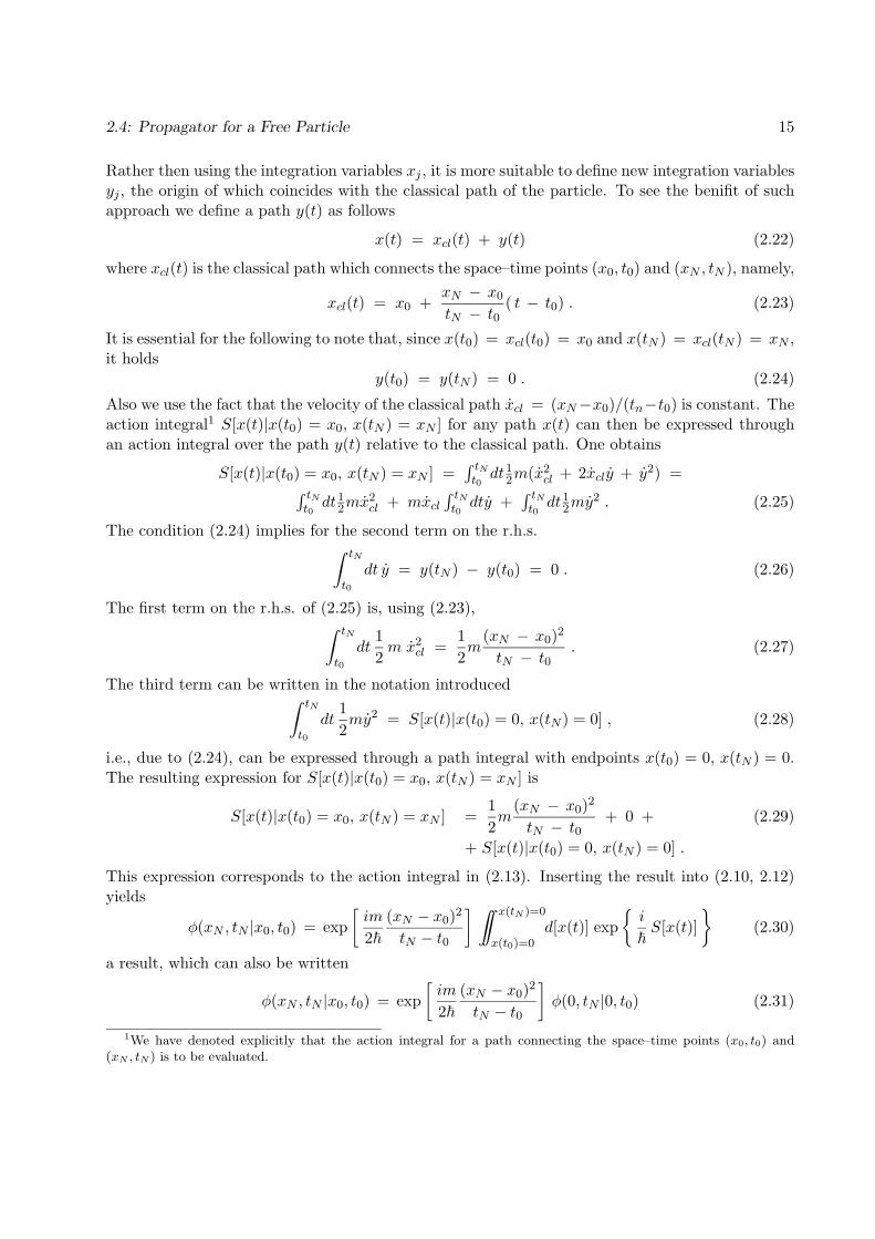
Rather then using the integration variables xj , it is more suitable to define new integration variablesyj , the origin of which coincides with the classical path of the particle. To see the benifit of suchapproach we define a path y(t) as follows
x(t) = xcl(t) + y(t) (2.22)
where xcl(t) is the classical path which connects the space–time points (x0, t0) and (xN , tN ), namely,
xcl(t) = x0 +xN − x0
tN − t0( t − t0) . (2.23)
It is essential for the following to note that, since x(t0) = xcl(t0) = x0 and x(tN ) = xcl(tN ) = xN ,it holds
y(t0) = y(tN ) = 0 . (2.24)
Also we use the fact that the velocity of the classical path xcl = (xN−x0)/(tn−t0) is constant. Theaction integral1 S[x(t)|x(t0) = x0, x(tN ) = xN ] for any path x(t) can then be expressed throughan action integral over the path y(t) relative to the classical path. One obtains
S[x(t)|x(t0) = x0, x(tN ) = xN ] =∫ tNt0dt1
2m(x2cl + 2xcly + y2) =∫ tN
t0dt1
2mx2cl + mxcl
∫ tNt0dty +
∫ tNt0dt1
2my2 . (2.25)
The condition (2.24) implies for the second term on the r.h.s.∫ tN
t0
dt y = y(tN ) − y(t0) = 0 . (2.26)
The first term on the r.h.s. of (2.25) is, using (2.23),∫ tN
t0
dt12m x2
cl =12m
(xN − x0)2
tN − t0. (2.27)
The third term can be written in the notation introduced∫ tN
t0
dt12my2 = S[x(t)|x(t0) = 0, x(tN ) = 0] , (2.28)
i.e., due to (2.24), can be expressed through a path integral with endpoints x(t0) = 0, x(tN ) = 0.The resulting expression for S[x(t)|x(t0) = x0, x(tN ) = xN ] is
S[x(t)|x(t0) = x0, x(tN ) = xN ] =12m
(xN − x0)2
tN − t0+ 0 + (2.29)
+ S[x(t)|x(t0) = 0, x(tN ) = 0] .
This expression corresponds to the action integral in (2.13). Inserting the result into (2.10, 2.12)yields
φ(xN , tN |x0, t0) = exp[im
2~(xN − x0)2
tN − t0
] ∫∫ x(tN )=0
x(t0)=0d[x(t)] exp
i
~
S[x(t)]
(2.30)
a result, which can also be written
φ(xN , tN |x0, t0) = exp[im
2~(xN − x0)2
tN − t0
]φ(0, tN |0, t0) (2.31)
1We have denoted explicitly that the action integral for a path connecting the space–time points (x0, t0) and(xN , tN ) is to be evaluated.

16 Quantum Mechanical Path Integral
Evaluation of the necessary path integral
To determine the propagator (2.31) for a free particle one needs to evaluate the following pathintegral
φ(0, tN |0, t0) = limN→∞
[m
2πi~εN
]N2 ×
×∫ +∞−∞ dy1 · · ·
∫ +∞−∞ dyN−1 exp
[i~εN∑N−1
j=012m
(yj+1− yj)2
ε2N
](2.32)
The exponent E can be written, noting y0 = yN = 0, as the quadratic form
E =im
2~εN( 2y2
1 − y1y2 − y2y1 + 2y22 − y2y3 − y3y2
+ 2y23 − · · · − yN−2yN−1 − yN−1yN−2 + 2y2
N−1 )
= i
N−1∑j,k=1
yj ajk yk (2.33)
where ajk are the elements of the following symmetric (N − 1)× (N − 1) matrix
(ajk
)=
m
2~εN
2 −1 0 . . . 0 0−1 2 −1 . . . 0 0
0 −1 2 . . . 0 0...
......
. . ....
...0 0 0 . . . 2 −10 0 0 −1 2
(2.34)
The following integral
∫ +∞
−∞dy1 · · ·
∫ +∞
−∞dyN−1 exp
i N−1∑j,k=1
yjajkyk
(2.35)
must be determined. In the appendix we prove
∫ +∞
−∞dy1 · · ·
∫ +∞
−∞dyN−1 exp
i d∑j,k=1
yjbjkyk
=[
(iπ)d
det(bjk)
] 12
. (2.36)
which holds for a d-dimensional, real, symmetric matrix (bjk) and det(bjk) 6= 0.In order to complete the evaluation of (2.32) we split off the factor m
2~εNin the definition (2.34) of
(ajk) defining a new matrix (Ajk) through
ajk =m
2~εNAjk . (2.37)
Using
det(ajk) =[m
2~εN
]N−1
det(Ajk) , (2.38)
2.4: Propagator for a Free Particle 17
a property which follows from det(cB) = cndetB for any n× n matrix B, we obtain
φ(0, tN |0, t0) = limN→∞
[m
2πi~εN
]N2[
2πi~εNm
]N−12 1√
det(Ajk). (2.39)
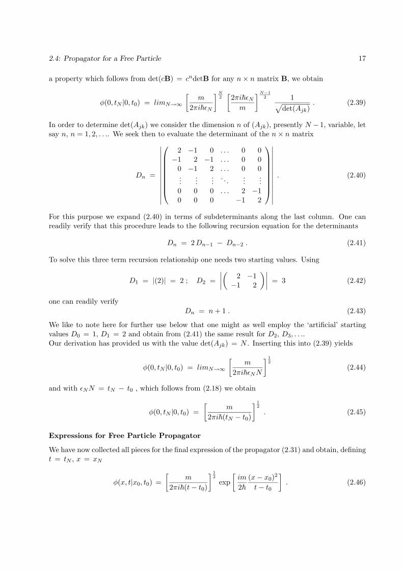
In order to determine det(Ajk) we consider the dimension n of (Ajk), presently N − 1, variable, letsay n, n = 1, 2, . . .. We seek then to evaluate the determinant of the n× n matrix
Dn =
∣∣∣∣∣∣∣∣∣∣∣∣∣
2 −1 0 . . . 0 0−1 2 −1 . . . 0 0
0 −1 2 . . . 0 0...
......
. . ....
...0 0 0 . . . 2 −10 0 0 −1 2
∣∣∣∣∣∣∣∣∣∣∣∣∣. (2.40)
For this purpose we expand (2.40) in terms of subdeterminants along the last column. One canreadily verify that this procedure leads to the following recursion equation for the determinants
Dn = 2Dn−1 − Dn−2 . (2.41)
To solve this three term recursion relationship one needs two starting values. Using
D1 = |(2)| = 2 ; D2 =∣∣∣∣( 2 −1−1 2
)∣∣∣∣ = 3 (2.42)
one can readily verifyDn = n+ 1 . (2.43)
We like to note here for further use below that one might as well employ the ‘artificial’ startingvalues D0 = 1, D1 = 2 and obtain from (2.41) the same result for D2, D3, . . ..Our derivation has provided us with the value det(Ajk) = N . Inserting this into (2.39) yields
φ(0, tN |0, t0) = limN→∞
[m
2πi~εNN
] 12
(2.44)
and with εNN = tN − t0 , which follows from (2.18) we obtain
φ(0, tN |0, t0) =[
m
2πi~(tN − t0)
] 12
. (2.45)
Expressions for Free Particle Propagator
We have now collected all pieces for the final expression of the propagator (2.31) and obtain, definingt = tN , x = xN
φ(x, t|x0, t0) =[
m
2πi~(t− t0)
] 12
exp[im
2~(x− x0)2
t− t0
]. (2.46)
18 Quantum Mechanical Path Integral
This propagator, according to (2.5) allows us to predict the time evolution of any state functionψ(x, t) of a free particle. Below we will apply this to a particle at rest and a particle forming aso-called wave packet.The result (2.46) can be generalized to three dimensions in a rather obvious way. One obtains thenfor the propagator (2.10)
φ(~r, t|~r0, t0) =[
m
2πi~(t− t0)
] 32
exp[im
2~(~r − ~r0)2
t− t0
]. (2.47)
One-Dimensional Free Particle Described by Wave Packet
We assume a particle at time t = to = 0 is described by the wave function
ψ(x0, t0) =[
1πδ2
] 14
exp(− x2
0
2δ2+ i
po~
x
)(2.48)
Obviously, the associated probability distribution
|ψ(x0, t0)|2 =[
1πδ2
] 12
exp(−x
20
δ2
)(2.49)
is Gaussian of width δ, centered around x0 = 0, and describes a single particle since[1πδ2
] 12∫ +∞
−∞dx0 exp
(−x
20
δ2
)= 1 . (2.50)
One refers to such states as wave packets. We want to apply axiom (2.5) to (2.48) as the initialstate using the propagator (2.46).We will obtain, thereby, the wave function of the particle at later times. We need to evaluate forthis purpose the integral
ψ(x, t) =[
1πδ2
] 14 [ m
2πi~t
] 12
∫ +∞
−∞dx0 exp
[im
2~(x− x0)2
t− x2
0
2δ2+ i
po~
xo
]︸ ︷︷ ︸
Eo(xo, x) + E(x)
(2.51)
For this evaluation we adopt the strategy of combining in the exponential the terms quadratic(∼ x2
0) and linear (∼ x0) in the integration variable to a complete square
ax20 + 2bx0 = a
(x0 +
b
a
)2
− b2
a(2.52)
and applying (2.247).We devide the contributions to the exponent Eo(xo, x) + E(x) in (2.51) as follows
Eo(xo, x) =im
2~t
[x2o
(1 + i
~t
mδ2
)− 2xo
(x − po
mt)
+ f(x)]
(2.53)
2.4: Propagator for a Free Particle 19
E(x) =im
2~t[x2 − f(x)
]. (2.54)
One chooses then f(x) to complete, according to (2.52), the square in (2.53)
f(x) =
x− pom t√
1 + i ~tmδ2
2
. (2.55)
This yields
Eo(xo, x) =im
2~t
xo
√1 + i
~t
mδ2−
x − pom t√
1 + i ~tmδ2
2
. (2.56)
One can write then (2.51)
ψ(x, t) =[
1πδ2
] 14 [ m
2πi~t
] 12eE(x)
∫ +∞
−∞dx0 e
Eo(xo,x) (2.57)
and needs to determine the integral
I =∫ +∞
−∞dx0 e
Eo(xo,x)
=∫ +∞
−∞dx0 exp
im
2~t
xo
√1 + i
~t
mδ2−
x − pom t√
1 + i ~tmδ2
2 =
∫ +∞
−∞dx0 exp
im
2~t
(1 + i
~t
mδ2
)(xo −
x − pom t
1 + i ~tmδ2
)2 . (2.58)
The integrand is an analytical function everywhere in the complex plane and we can alter the inte-gration path, making certain, however, that the new path does not lead to additional contributionsto the integral.We proceed as follows. We consider a transformation to a new integration variable ρ defined through√
i
(1 − i
~t
mδ2
)ρ = x0 −
x − pom t
1 + i ~tmδ2
. (2.59)
An integration path in the complex x0–plane along the direction√i
(1 − i
~t
mδ2
)(2.60)
is then represented by real ρ values. The beginning and the end of such path are the points
z′1 = −∞ ×
√i
(1 − i
~t
mδ2
), z′2 = +∞ ×
√i
(1 − i
~t
mδ2
)(2.61)

20 Quantum Mechanical Path Integral
whereas the original path in (2.58) has the end points
z1 = −∞ , z2 = +∞ . (2.62)
If one can show that an integration of (2.58) along the path z1 → z′1 and along the path z2 → z′2gives only vanishing contributions one can replace (2.58) by
I =
√i
(1 − i
~t
mδ2
) ∫ +∞
−∞dρ exp
[− m
2~t
(1 +
(~t
mδ2
)2)ρ2
](2.63)
which can be readily evaluated. In fact, one can show that z′1 lies at −∞ − i × ∞ and z′2 at+∞ + i×∞. Hence, the paths between z1 → z′1 and z2 → z′2 have a real part of x0 of ±∞. Sincethe exponent in (2.58) has a leading contribution in x0 of −x2
0/δ2 the integrand of (2.58) vanishes
for Rex0 → ±∞. We can conclude then that (2.63) holds and, accordingly,
I =
√2πi~t
m(1 + i ~tmδ2 )
. (2.64)
Equation (2.57) reads then
ψ(x, t) =[
1πδ2
] 14
[1
1 + i ~tmδ2
] 12
exp [E(x) ] . (2.65)
Seperating the phase factor [1 − i ~t
mδ2
1 + i ~tmδ2
] 14
, (2.66)
yields
ψ(x, t) =
[1 − i ~t
mδ2
1 + i ~tmδ2
] 14[
1πδ2 (1 + ~2t2
m2δ4 )
] 14
exp [E(x) ] . (2.67)
We need to determine finally (2.54) using (2.55). One obtains
E(x) = − x2
2δ2(1 + i ~tmδ2 )
+ipo~x
1 + i ~tmδ2
−i~
p2o
2m t
1 + i ~tmδ2
(2.68)
and, usinga
1 + b= a − a b
1 + b, (2.69)
finally
E(x) = −(x − po
m t)2
2δ2(1 + i ~tmδ2 )
+ ipo~
x − i
~
p2o
2mt (2.70)
2.4: Propagator for a Free Particle 21
which inserted in (2.67) provides the complete expression of the wave function at all times t
ψ(x, t) =
[1 − i ~t
mδ2
1 + i ~tmδ2
] 14[
1πδ2 (1 + ~2t2
m2δ4 )
] 14
× (2.71)
× exp
[−
(x − pom t)2
2δ2(1 + ~2t2
m2δ4 )(1 − i
~t
mδ2) + i
po~
x − i
~
p2o
2mt
].
The corresponding probability distribution is
|ψ(x, t)|2 =
[1
πδ2 (1 + ~2t2
m2δ4 )
] 12
exp
[−
(x − pom t)2
δ2(1 + ~2t2
m2δ4 )
]. (2.72)
Comparision of Moving Wave Packet with Classical Motion
It is revealing to compare the probability distributions (2.49), (2.72) for the initial state (2.48) andfor the final state (2.71), respectively. The center of the distribution (2.72) moves in the directionof the positive x-axis with velocity vo = po/m which identifies po as the momentum of the particle.The width of the distribution (2.72)
δ
√1 +
~2t2
m2δ4(2.73)
increases with time, coinciding at t = 0 with the width of the initial distribution (2.49). This‘spreading’ of the wave function is a genuine quantum phenomenon. Another interesting observationis that the wave function (2.71) conserves the phase factor exp[i(po/~)x] of the original wave function(2.48) and that the respective phase factor is related with the velocity of the classical particle andof the center of the distribution (2.72). The conservation of this factor is particularly striking forthe (unnormalized) initial wave function
ψ(x0, t0) = exp(ipomxo
), (2.74)
which corresponds to (2.48) for δ → ∞. In this case holds
ψ(x, t) = exp(ipomx − i
~
p2o
2mt
). (2.75)
i.e., the spatial dependence of the initial state (2.74) remains invariant in time. However, a time-dependent phase factor exp[− i
~(p2o/2m) t] arises which is related to the energy ε = p2
o/2m of aparticle with momentum po. We had assumed above [c.f. (2.48)] to = 0. the case of arbitrary to isrecovered iby replacing t → to in (2.71, 2.72). This yields, instead of (2.75)
ψ(x, t) = exp(ipomx − i
~
p2o
2m(t − to)
). (2.76)
From this we conclude that an initial wave function
ψ(xo, t0) = exp(ipomxo −
i
~
p2o
2mto
). (2.77)
22 Quantum Mechanical Path Integral
becomes at t > to
ψ(x, t) = exp(ipomx − i
~
p2o
2mt
), (2.78)
i.e., the spatial as well as the temporal dependence of the wave function remains invariant in thiscase. One refers to the respective states as stationary states. Such states play a cardinal role inquantum mechanics.
2.5 Propagator for a Quadratic Lagrangian
We will now determine the propagator (2.10, 2.12, 2.13)
φ(xN , tN |x0, t0) =∫∫ x(tN )=xN
x(t0)=x0
d[x(t)] expi
~
S[x(t)]
(2.79)
for a quadratic Lagrangian
L(x, x, t) =12mx2 − 1
2c(t)x2 − e(t)x . (2.80)
For this purpose we need to determine the action integral
S[x(t)] =∫ tN
t0
dt′ L(x, x, t) (2.81)
for an arbitrary path x(t) with end points x(t0) = x0 and x(tN ) = xN . In order to simplify thistask we define again a new path y(t)
x(t) = xcl(t) + y(t) (2.82)
which describes the deviation from the classical path xcl(t) with end points xcl(t0) = x0 andxcl(tN ) = xN . Obviously, the end points of y(t) are
y(t0) = 0 ; y(tN ) = 0 . (2.83)
Inserting (2.80) into (2.82) one obtains
L(xcl + y, xcl + y(t), t) = L(xcl, xcl, t) + L′(y, y(t), t) + δL (2.84)
where
L(xcl, xcl, t) =12mx2
cl −12c(t)x2
cl − e(t)xcl
L′(y, y(t), t) =12my2 − 1
2c(t)y2
δL = mxcly(t) − c(t)xcly − e(t)y . (2.85)
We want to show now that the contribution of δL to the action integral (2.81) vanishes2. For thispurpose we use
xcly =d
dt(xcl y) − xcl y (2.86)
2The reader may want to verify that the contribution of δL to the action integral is actually equal to the differentialδS[xcl, y(t)] which vanishes according to the Hamiltonian principle as discussed in Sect. 1.
2.5: Propagator for a Quadratic Lagrangian 23
and obtain ∫ tN
t0
dt δL = m [xcl y]|tN
t0−∫ tN
t0
dt [mxcl(t) + c(t)xcl(t) + e(t) ] y(t) . (2.87)
According to (2.83) the first term on the r.h.s. vanishes. Applying the Euler–Lagrange conditions(1.24) to the Lagrangian (2.80) yields for the classical path
mxcl + c(t)xcl + e(t) = 0 (2.88)
and, hence, also the second contribution on the r.h.s. of (2.88) vanishes. One can then express thepropagator (2.79)
φ(xN , tN |x0, t0) = expi
~
S[xcl(t)]φ(0, tN |0, t0) (2.89)
where
φ(0, tN |0, t0) =∫∫ y(tN )=0
y(t0)=0d[y(t)] exp
i
~
∫ tN
t0
dtL′(y, y, t). (2.90)
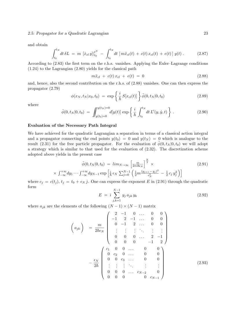
Evaluation of the Necessary Path Integral
We have achieved for the quadratic Lagrangian a separation in terms of a classical action integraland a propagator connecting the end points y(t0) = 0 and y(tN ) = 0 which is analogue to theresult (2.31) for the free particle propagator. For the evaluation of φ(0, tN |0, t0) we will adopta strategy which is similar to that used for the evaluation of (2.32). The discretization schemeadopted above yields in the present case
φ(0, tN |0, t0) = limN→∞
[m
2πi~εN
]N2 × (2.91)
×∫ +∞−∞ dy1 · · ·
∫ +∞−∞ dyN−1 exp
[i~εN∑N−1
j=0
(12m
(yj+1− yj)2
ε2N− 1
2 cj y2j
)]where cj = c(tj), tj = t0 + εN j. One can express the exponent E in (2.91) through the quadraticform
E = i
N−1∑j,k=1
yj ajk yk (2.92)
where ajk are the elements of the following (N − 1)× (N − 1) matrix
(ajk
)=
m
2~εN
2 −1 0 . . . 0 0−1 2 −1 . . . 0 0
0 −1 2 . . . 0 0...
......
. . ....
...0 0 0 . . . 2 −10 0 0 −1 2
− εN2~
c1 0 0 . . . 0 00 c2 0 . . . 0 00 0 c3 . . . 0 0...
......
. . ....
...0 0 0 . . . cN−2 00 0 0 0 cN−1
(2.93)

24 Quantum Mechanical Path Integral
In case det(ajk) 6= 0 one can express the multiple integral in (2.91) according to (2.36) as follows
φ(0, tN |0, t0) = limN→∞
[m
2πi~εN
]N2[
(iπ)N−1
det(a)
] 12
= limN→∞
m
2πi~1
εN
(2~εNm
)N−1det(a)
12
. (2.94)
In order to determine φ(0, tN |0, t0) we need to evaluate the function
f(t0, tN ) = limN→∞
[εN
(2~εNm
)N−1
det(a)
]. (2.95)
According to (2.93) holds
DN−1def=
[2~εNm
]N−1det(a) (2.96)
=
∣∣∣∣∣∣∣∣∣∣∣∣∣∣∣∣
2− ε2Nm c1 −1 0 . . . 0 0
−1 2− ε2Nm c2 −1 . . . 0 0
0 −1 2− ε2Nm c3 . . . 0 0
......
.... . .
......
0 0 0 . . . 2− ε2Nm cN−2 −1
0 0 0 −1 2− ε2Nm cN−1
∣∣∣∣∣∣∣∣∣∣∣∣∣∣∣∣In the following we will asume that the dimension n = N − 1 of the matrix in (2.97) is variable.One can derive then for Dn the recursion relationship
Dn =(
2 −ε2Nmcn
)Dn−1 − Dn−2 (2.97)
using the well-known method of expanding a determinant in terms of the determinants of lowerdimensional submatrices. Using the starting values [c.f. the comment below Eq. (2.43)]
D0 = 1 ; D1 = 2 −ε2Nm
c1 (2.98)
this recursion relationship can be employed to determine DN−1. One can express (2.97) throughthe 2nd order difference equation
Dn+1 − 2Dn + Dn−1
ε2N= − cn+1Dn
m. (2.99)
Since we are interested in the solution of this equation in the limit of vanishing εN we may interpret(2.99) as a 2nd order differential equation in the continuous variable t = nεN + t0
d2f(t0, t)dt2
= − c(t)m
f(t0, t) . (2.100)
2.5: Propagator for a Quadratic Lagrangian 25
The boundary conditions at t = t0, according to (2.98), are
f(t0, t0) = εN D0 = 0 ;
df(t0,t)dt
∣∣∣t=t0
= εND1 −D0
εN= 2 −
ε2Nm
c1 − 1 = 1 . (2.101)
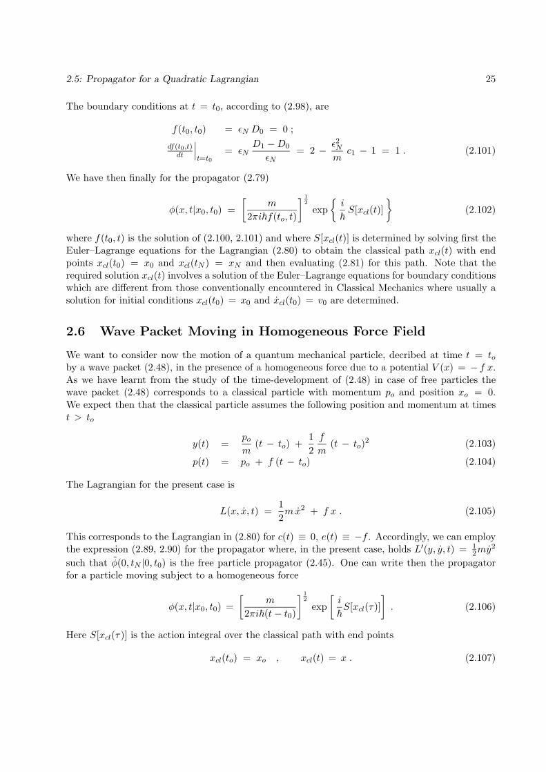
We have then finally for the propagator (2.79)
φ(x, t|x0, t0) =[
m
2πi~f(to, t)
] 12
expi
~
S[xcl(t)]
(2.102)
where f(t0, t) is the solution of (2.100, 2.101) and where S[xcl(t)] is determined by solving first theEuler–Lagrange equations for the Lagrangian (2.80) to obtain the classical path xcl(t) with endpoints xcl(t0) = x0 and xcl(tN ) = xN and then evaluating (2.81) for this path. Note that therequired solution xcl(t) involves a solution of the Euler–Lagrange equations for boundary conditionswhich are different from those conventionally encountered in Classical Mechanics where usually asolution for initial conditions xcl(t0) = x0 and xcl(t0) = v0 are determined.
2.6 Wave Packet Moving in Homogeneous Force Field
We want to consider now the motion of a quantum mechanical particle, decribed at time t = toby a wave packet (2.48), in the presence of a homogeneous force due to a potential V (x) = − f x.As we have learnt from the study of the time-development of (2.48) in case of free particles thewave packet (2.48) corresponds to a classical particle with momentum po and position xo = 0.We expect then that the classical particle assumes the following position and momentum at timest > to
y(t) =pom
(t − to) +12f
m(t − to)2 (2.103)
p(t) = po + f (t − to) (2.104)
The Lagrangian for the present case is
L(x, x, t) =12mx2 + f x . (2.105)
This corresponds to the Lagrangian in (2.80) for c(t) ≡ 0, e(t) ≡ −f . Accordingly, we can employthe expression (2.89, 2.90) for the propagator where, in the present case, holds L′(y, y, t) = 1
2my2
such that φ(0, tN |0, t0) is the free particle propagator (2.45). One can write then the propagatorfor a particle moving subject to a homogeneous force
φ(x, t|x0, t0) =[
m
2πi~(t− t0)
] 12
exp[i
~
S[xcl(τ)]]. (2.106)
Here S[xcl(τ)] is the action integral over the classical path with end points
xcl(to) = xo , xcl(t) = x . (2.107)
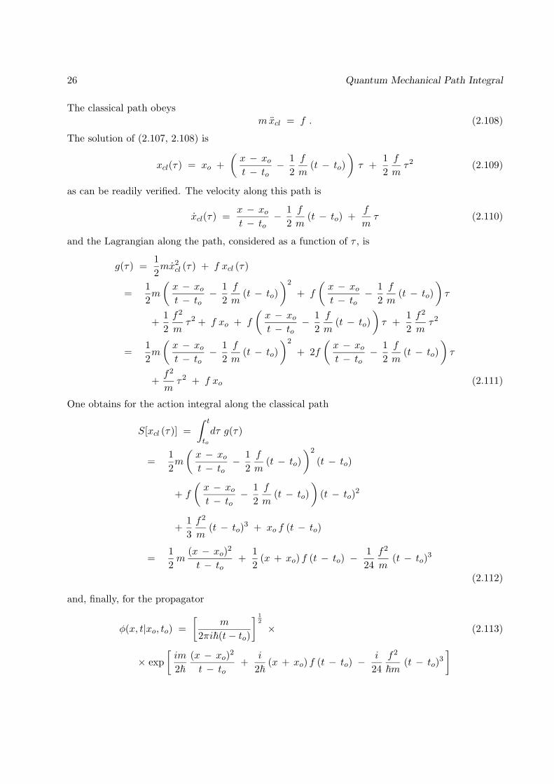
26 Quantum Mechanical Path Integral
The classical path obeysmxcl = f . (2.108)
The solution of (2.107, 2.108) is
xcl(τ) = xo +(x − xot − to
− 12f
m(t − to)
)τ +
12f
mτ2 (2.109)
as can be readily verified. The velocity along this path is
xcl(τ) =x − xot − to
− 12f
m(t − to) +
f
mτ (2.110)
and the Lagrangian along the path, considered as a function of τ , is
g(τ) =12mx2
cl (τ) + f xcl (τ)
=12m
(x − xot − to
− 12f
m(t − to)
)2
+ f
(x − xot − to
− 12f
m(t − to)
)τ
+12f2
mτ2 + f xo + f
(x − xot − to
− 12f
m(t − to)
)τ +
12f2
mτ2
=12m
(x − xot − to
− 12f
m(t − to)
)2
+ 2f(x − xot − to
− 12f
m(t − to)
)τ
+f2
mτ2 + f xo (2.111)
One obtains for the action integral along the classical path
S[xcl (τ)] =∫ t
to
dτ g(τ)
=12m
(x − xot − to
− 12f
m(t − to)
)2
(t − to)
+ f
(x − xot − to
− 12f
m(t − to)
)(t − to)2
+13f2
m(t − to)3 + xo f (t − to)
=12m
(x − xo)2
t − to+
12
(x + xo) f (t − to) −124
f2
m(t − to)3
(2.112)
and, finally, for the propagator
φ(x, t|xo, to) =[
m
2πi~(t− to)
] 12
× (2.113)
× exp[im
2~(x − xo)2
t − to+
i
2~(x + xo) f (t − to) −
i
24f2
~m(t − to)3
]
2.5: Propagator for a Quadratic Lagrangian 27
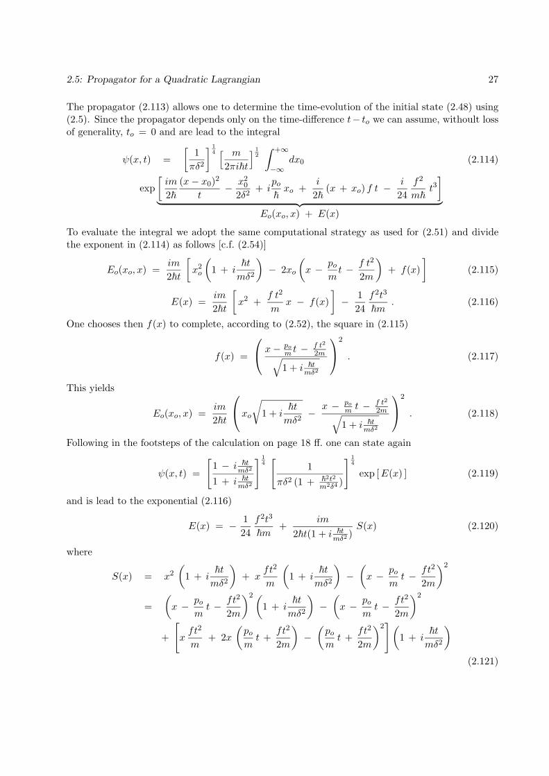
The propagator (2.113) allows one to determine the time-evolution of the initial state (2.48) using(2.5). Since the propagator depends only on the time-difference t− to we can assume, withoult lossof generality, to = 0 and are lead to the integral
ψ(x, t) =[
1πδ2
] 14 [ m
2πi~t
] 12
∫ +∞
−∞dx0 (2.114)
exp[im
2~(x− x0)2
t− x2
0
2δ2+ i
po~
xo +i
2~(x + xo) f t −
i
24f2
m~t3]
︸ ︷︷ ︸Eo(xo, x) + E(x)
To evaluate the integral we adopt the same computational strategy as used for (2.51) and dividethe exponent in (2.114) as follows [c.f. (2.54)]
Eo(xo, x) =im
2~t
[x2o
(1 + i
~t
mδ2
)− 2xo
(x − po
mt − f t2
2m
)+ f(x)
](2.115)
E(x) =im
2~t
[x2 +
f t2
mx − f(x)
]− 1
24f2t3
~m. (2.116)
One chooses then f(x) to complete, according to (2.52), the square in (2.115)
f(x) =
x− pom t −
f t2
2m√1 + i ~t
mδ2
2
. (2.117)
This yields
Eo(xo, x) =im
2~t
xo
√1 + i
~t
mδ2−
x − pom t − f t2
2m√1 + i ~t
mδ2
2
. (2.118)
Following in the footsteps of the calculation on page 18 ff. one can state again
ψ(x, t) =
[1 − i ~t
mδ2
1 + i ~tmδ2
] 14[
1πδ2 (1 + ~2t2
m2δ4 )
] 14
exp [E(x) ] (2.119)
and is lead to the exponential (2.116)
E(x) = − 124
f2t3
~m+
im
2~t(1 + i ~tmδ2 )
S(x) (2.120)
where
S(x) = x2
(1 + i
~t
mδ2
)+ x
ft2
m
(1 + i
~t
mδ2
)−(x − po
mt − ft2
2m
)2
=(x − po
mt − ft2
2m
)2(1 + i
~t
mδ2
)−(x − po
mt − ft2
2m
)2
+
[xft2
m+ 2x
(pomt +
ft2
2m
)−(pomt +
ft2
2m
)2](
1 + i~t
mδ2
)(2.121)
28 Quantum Mechanical Path Integral
Inserting this into (2.120) yields
E(x) = −
(x − po
m t − ft2
2m
)2
2δ2(1 + i ~t
mδ2
) (2.122)
+i
~
(po + f t)x − i
2m~
(pot + poft
2 +f2t3
4+f2t3
12
)The last term can be written
− i
2m~
(pot + poft
2 +f2t3
3
)= − i
2m~
∫ t
0dτ (po + fτ)2 . (2.123)
Altogether, (2.119, 2.122, 2.123) provide the state of the particle at time t > 0
ψ(x, t) =
[1 − i ~t
mδ2
1 + i ~tmδ2
] 14[
1πδ2 (1 + ~2t2
m2δ4 )
] 14
×
× exp
−(x − po
m t − ft2
2m
)2
2δ2(
1 + ~2t2
m2δ4
) (1 − i
~t
mδ2
) ×× exp
[i
~
(po + f t)x − i
~
∫ t
0dτ
(po + fτ)2
2m
]. (2.124)
The corresponding probablity distribution is
|ψ(x, t)|2 =
[1
πδ2 (1 + ~2t2
m2δ4 )
] 12
exp
−(x − po
m t − ft2
2m
)2
δ2(
1 + ~2t2
m2δ4
) . (2.125)
Comparision of Moving Wave Packet with Classical Motion
It is again [c.f. (2.4)] revealing to compare the probability distributions for the initial state (2.48)and for the states at time t, i.e., (2.125). Both distributions are Gaussians. Distribution (2.125)moves along the x-axis with distribution centers positioned at y(t) given by (2.103), i.e., as expectedfor a classical particle. The states (2.124), in analogy to the states (2.71) for free particles, exhibit aphase factor exp[ip(t)x/~], for which p(t) agrees with the classical momentum (2.104). While theseproperties show a close correspondence between classical and quantum mechanical behaviour, thedistribution shows also a pure quantum effect, in that it increases its width . This increase, forthe homogeneous force case, is identical to the increase (2.73) determined for a free particle. Suchincrease of the width of a distribution is not a necessity in quantum mechanics. In fact, in case of so-called bound states, i.e., states in which the classical and quantum mechanical motion is confined toa finite spatial volume, states can exist which do not alter their spatial distribution in time. Suchstates are called stationary states. In case of a harmonic potential there exists furthermore thepossibility that the center of a wave packet follows the classical behaviour and the width remainsconstant in time. Such states are referred to as coherent states, or Glauber states, and will be
2.5: Propagator for a Quadratic Lagrangian 29
studied below. It should be pointed out that in case of vanishing, linear and quadratic potentialsquantum mechanical wave packets exhibit a particularly simple evolution; in case of other type ofpotential functions and, in particular, in case of higher-dimensional motion, the quantum behaviourcan show features which are much more distinctive from classical behaviour, e.g., tunneling andinterference effects.
Propagator of a Harmonic Oscillator
In order to illustrate the evaluation of (2.102) we consider the case of a harmonic oscillator. Inthis case holds for the coefficents in the Lagrangian (2.80) c(t) = mω2 and e(t) = 0, i.e., theLagrangian is
L(x, x) =12mx2 − 1
2mω2x2 . (2.126)
.We determine first f(t0, t). In the present case holds
f = −ω2f ; f(t0, t0) = 0 ; f(to, to) = 1 . (2.127)
The solution which obeys the stated boundary conditions is
f(t0, t) =sinω(t − t0)
ω. (2.128)
We determine now S[xcl(τ)]. For this purpose we seek first the path xcl(τ) which obeys xcl(t0) = x0
and xcl(t) = x and satisfies the Euler–Lagrange equation for the harmonic oscillator
mxcl + mω2 xcl = 0 . (2.129)
This equation can be writtenxcl = −ω2 xcl . (2.130)
the general solution of which is
xcl(τ ′) = A sinω(τ − t0) + B cosω(τ − t0) . (2.131)
The boundary conditions xcl(t0) = x0 and xcl(t) = x are satisfied for
B = x0 ; A =x − x0 cosω(t− to)
sinω(t − t0), (2.132)
and the desired path is
xcl(τ) =x − x0 c
ssinω(τ − t0) + x0 cosω(τ − t0) (2.133)
where we introducedc = cosω(t− to) , s = sinω(t− to) (2.134)
We want to determine now the action integral associated with the path (2.133, 2.134)
S[xcl(τ)] =∫ t
t0
dτ
(12mx2
cl(τ) − 12mω2x2
cl(τ))
(2.135)

30 Quantum Mechanical Path Integral
For this purpose we assume presently to = 0. From (2.133) follows for the velocity along theclassical path
xcl(τ) = ωx − x0 c
scosωτ − ω x0 sinωτ (2.136)
and for the kinetic energy
12mx2
cl(τ) =12mω2 (x − x0 c)2
s2cos2ωτ
−mω2xox − x0 c
scosωτ sinωτ
+12mω2 x2
o sin2ωτ (2.137)
Similarly, one obtains from (2.133) for the potential energy
12mω2x2
cl(τ) =12mω2 (x − x0 c)2
s2sin2ωτ
+mω2xox − x0 c
scosωτ sinωτ
+12mω2 x2
o cos2ωτ (2.138)
Using
cos2ωτ =12
+12
cos2ωτ (2.139)
sin2ωτ =12− 1
2cos2ωτ (2.140)
cosωτ sinωτ =12
sin2ωτ (2.141)
the Lagrangian, considered as a function of τ , reads
g(τ) =12mx2
cl(τ) − 12mω2x2
cl(τ) =12mω2 (x − x0 c)2
s2cos2ωτ
−mω2xox − x0 c
ssin2ωτ
−12mω2 x2
o cos2ωτ (2.142)
Evaluation of the action integral (2.135), i.e., of S[xcl(τ)] =∫ t
0dτg(τ) requires the integrals∫ t
0dτcos2ωτ =
12ω
sin2ωt =1ωs c (2.143)∫ t
0dτsin2ωτ =
12ω
[ 1 − cos2ωt ] =1ωs2 (2.144)
where we employed the definition (2.134) Hence, (2.135) is, using s2 + c2 = 1,
S[xcl(τ)] =12mω
(x − x0 c)2
s2s c − mωxo
x − x0 c
ss2 − 1
2mω2 x2
o s c
=mω
2s[
(x2 − 2xxoc+ x2oc
2) c − 2xoxs2 + 2x2ocs
2 − x2os
2c]
=mω
2s[
(x2 + x2o) c − 2xox
](2.145)
2.5: Propagator for a Quadratic Lagrangian 31
and, with the definitions (2.134),
S[xcl(τ)] =mω
2sinω(t − t0)[(x2
0 + x2) cosω(t − t0) − 2x0x]. (2.146)
For the propagator of the harmonic oscillator holds then
φ(x, t|x0, t0) =[
mω2πi~ sinω(t− t0)
] 12 ×
× exp
imω2~ sinω(t− t0)
[(x2
0 + x2) cosω(t − t0) − 2x0x]
. (2.147)
Quantum Pendulum or Coherent States
As a demonstration of the application of the propagator (2.147) we use it to describe the timedevelopment of the wave function for a particle in an initial state
ψ(x0, t0) =[mωπ~
] 14 exp
(− mω(x0 − bo)2
2~+
i
~
po xo
). (2.148)
The initial state is decribed by a Gaussian wave packet centered around the position x = bo andcorresponds to a particle with initial momentum po. The latter property follows from the role ofsuch factor for the initial state (2.48) when applied to the case of a free particle [c.f. (2.71)] or tothe case of a particle moving in a homogeneous force [c.f. (2.124, 2.125)] and will be borne out ofthe following analysis; at present one may regard it as an assumption.If one identifies the center of the wave packet with a classical particle, the following holds for thetime development of the position (displacement), momentum, and energy of the particle
b(t) = bo cosω(t− to) +pomω
sinω(t− to) displacement
p(t) = −mωbo sinω(t− to) + po cosω(t− to) momentum
εo =p2o
2m+ 1
2mω2b2o energy
(2.149)
We want to explore, using (2.5), how the probability distribution |ψ(x, t)|2 of the quantum particlepropagates in time.The wave function at times t > t0 is
ψ(x, t) =∫ ∞−∞
dx0 φ(x, t|x0, t0)ψ(x0, t0) . (2.150)
Expressing the exponent in (2.148)
imω
2~sinω(t− to)
[i (xo − bo)2 sinω(t− to) +
2pomω
xo sinω(t− to)]
(2.151)
(2.147, 2.150, 2.151) can be written
ψ(x, t) =[mωπ~
] 14
[m
2πiω~sinω(t − t0)
] 12∫ ∞−∞
dx0 exp [E0 + E ] (2.152)
32 Quantum Mechanical Path Integral
where
E0(xo, x) =imω
2~s
[x2oc − 2xox + isx2
o − 2isxobo +2pomω
xos + f(x)]
(2.153)
E(x) =imω
2~s[x2c + isb2o − f(x)
]. (2.154)
c = cosω(t − to) , s = sinω(t − to) . (2.155)
Here f(x) is a function which is introduced to complete the square in (2.153) for simplification ofthe Gaussian integral in x0. Since E(x) is independent of xo (2.152) becomes
ψ(x, t) =[mωπ~
] 14
[m
2πiω~sinω(t − t0)
] 12
eE(x)
∫ ∞−∞
dx0 exp [E0(xo, x)] (2.156)
We want to determine now Eo(xo, x) as given in (2.153). It holds
Eo =imω
2~s
[x2o e
iω(t−to) − 2xo(x+ isbo −pomω
s) + f(x)]
(2.157)
For f(x) to complete the square we choose
f(x) = (x + isbo −pomω
s)2 e−iω(t−to) . (2.158)
One obtains for (2.157)
E0(xo, x) =imω
2~sexp [iω(t− t0)]
[x0 − (x+ isbo −
pomω
s) exp (−iω(t− t0)]2
. (2.159)
To determine the integral in (2.156) we employ the integration formula (2.247) and obtain∫ +∞
−∞dx0 e
E0(x0) =[
2πi~ sinω(t− t0)mω exp[iω(t− t0)]
] 12
(2.160)
Inserting this into (2.156) yields
ψ(x, t) =[mωπ~
] 14eE(x) (2.161)
For E(x) as defined in (2.154) one obtains, using exp[±iω(t− to)] = c ± is,
E(x) = imω2~s
[x2c + isb2o − x2c + isx2 − 2isxboc − 2s2xbo
+ s2b2oc − is3b2o + 2 pomω xsc + 2i po
mω bos2c
− 2i pomω xs
2 + 2 pomω bos
3 − p2o
m2ω2 s2c + i p2
om2ω2 s
3]
= − mω2~
[x2 + c2b2o − 2xboc + 2ixsbo − ib2osc
−2 pomω xs + 2 po
mω bosc + p2o
m2ω2 s2 − 2i po
mω xc
−2i pomω bos
2 + i p2o
m2ω2 sc]
= − mω2~ (x − cbo − po
mω s)2 +
i
~
(−mωbos + poc)x
− i
~
( p2o
2mω −12mωb
2o)sc +
i
~
pobos2 (2.162)

2.5: Propagator for a Quadratic Lagrangian 33
We note the following identities∫ t
to
dτp2(τ)2m
=12εo(t− to) +
12
(p2o
2mω− mωb2o
2
)sc − 1
2bopos
2 (2.163)∫ t
to
dτmω2b2(τ)
2
=12εo(t− to) −
12
(p2o
2mω− mωb2o
2
)sc +
12bopos
2 (2.164)
where we employed b(τ) and p(τ) as defined in (2.149). From this follows, using p(τ) = mb(τ) andthe Lagrangian (2.126),∫ t
to
dτ L[b(τ), b(τ)] =(
p2o
2mω− mωb2o
2
)sc − bopos (2.165)
such that E(x) in (2.162) can be written, using again (2.149)),
E(x) = − mω2~
[x− b(t)]2 +i
~
p(t)x − i12ω (t− to) −
i
~
∫ t
to
dτ L[b(τ), b(τ)] (2.166)
Inserting this into (2.161) yields,
ψ(x, t) =[mωπ~
] 14 × exp
− mω
2~[x− b(t)]2
× (2.167)
× expi
~
p(t)x − i12ω (t− to) −
i
~
∫ t
to
dτ L[b(τ), b(τ)]
where b(t), p(t), and εo are the classical displacement, momentum and energy, respectively, definedin (2.149).
Comparision of Moving Wave Packet with Classical Motion
The probability distribution associated with (2.167)
|ψ(x, t)|2 =[mωπ~
] 12 exp
−mω~
[x − b(t)]2
(2.168)
is a Gaussian of time-independent width, the center of which moves as described by b(t) given in(2.148) , i.e., the center follows the motion of a classical oscillator (pendulum) with initial positionbo and initial momentum po. It is of interest to recall that propagating wave packets in the case ofvanishing [c.f. (2.72)] or linear [c.f. (2.125)] potentials exhibit an increase of their width in time; incase of the quantum oscillator for the particular width chosen for the initial state (2.148) the width,actually, is conserved. One can explain this behaviour as arising from constructive interference dueto the restoring forces of the harmonic oscillator. We will show in Chapter 4 [c.f. (4.166, 4.178) andFig. 4.1] that an initial state of arbitrary width propagates as a Gaussian with oscillating width.

34 Quantum Mechanical Path Integral
In case of the free particle wave packet (2.48, 2.71) the factor exp(ipox) gives rise to the transla-tional motion of the wave packet described by pot/m, i.e., po also corresponds to initial classicalmomentum. In case of a homogeneous force field the phase factor exp(ipox) for the initial state(2.48) gives rise to a motion of the center of the propagating wave packet [c.f. (2.125)] described by(po/m)t + 1
2ft2 such that again po corresponds to the classical momentum. Similarly, one observes
for all three cases (free particle, linear and quadratic potential) a phase factor exp[ip(t)x/~] for thepropagating wave packet where fp(t) corresponds to the initial classical momentum at time t. Onecan, hence, summarize that for the three cases studied (free particle, linear and quadratic potential)propagating wave packets show remarkably close analogies to classical motion.We like to consider finally the propagation of an initial state as in (2.148), but with bo = 0 andpo = 0. Such state is given by the wave function
ψ(x0, t0) =[mωπ~
] 14 exp
(− mωx
20
2~− iω
2to
). (2.169)
where we added a phase factor exp(−iωto/2). According to (2.167) the state (2.169) reproducesitself at later times t and the probablity distribution remains at all times equal to[mω
π~
] 12 exp
(− mωx
20
~
), (2.170)
i.e., the state (2.169) is a stationary state of the system. The question arises if the quantumoscillator posesses further stationary states. In fact, there exist an infinite number of such stateswhich will be determined now.
2.7 Stationary States of the Harmonic Oscillator
In order to find the stationary states of the quantum oscillator we consider the function
W (x, t) = exp(
2√mω
~
x e−iωt − e−2iωt − mω
2~x2 − iωt
2
). (2.171)
We want to demonstrate that w(x, t) is invariant in time, i.e., for the propagator (2.147) of theharmonic oscillator holds
W (x, t) =∫ +∞
−∞dxo φ(x, t|xo, to)W (xo, to) . (2.172)
We will demonstrate further below that (2.172) provides us in a nutshell with all the stationarystates of the harmonic oscillator, i.e., with all the states with time-independent probability distri-bution.In order to prove (2.172) we express the propagator, using (2.147) and the notation T = t− to
φ(x, t|xo, to) = e−12iωT
[mω
π~(1− e−2iωT )
] 12
×
× exp[−mω
2~(x2o + x2)
1 + e−2iωT
1 − e−2iωT− mω
~ω
2xxoe−iωT
1 − e−2iωT
](2.173)

2.5: Propagator for a Quadratic Lagrangian 35
One can write then the r.h.s. of (2.172)
I = e−12iωt
[mω
π~(1− e−2iωT )
] 12∫ +∞
−∞dxo exp[Eo(xo, x) + E(x) ] (2.174)
where
Eo(xo, x) = − mω2~
[x2o
(1 + e−2iωT
1− e−2iωT+ 1)
(2.175)
+ 2xo
(2xe−iωT
1− e−2iωT+ 2
√~
mωe−iωto
)+ f(x)
]
E(x) = − mω2~
[x2 1 + e−2iωT
1− e−2iωT+
2~mω
e−2iωto − f(x)]
(2.176)
Following the by now familiar strategy one choses f(x) to complete the square in (2.175), namely,
f(x) =12
(1 − e−2iωT )
(2xe−iωT
1− e−2iωT+ 2
√~
mωe−iωto
)2
. (2.177)
This choice of f(x) results in
Eo(xo, x) = − mω2~
[xo
√2
1− e−2iωT
+
√1− e−2iωT
2
(2xe−iωT
1− e−2iωT+ 2
√~
mωe−iωto
)]2
= imω
i~(e−2iωT − 1)(xo + zo)2 (2.178)
for some constant zo ∈ C. Using (2.247) one obtains∫ +∞
−∞dxo e
Eo(xo,x) =[π~(1 − e−2iωT
mω
] 12
(2.179)
and, therefore, one obtains for (2.174)
I = e−12iωt eE(x) . (2.180)
For E(x), as given in (2.176, 2.177), holds
E(x) = − mω2~
[x2 1 + e−2iωT
1− e−2iωT+
2~mω
e−2iωto − 2x2e−2iωT
1− e−2iωT
−4
√~
mωxe−iωT − 2 (1− e−2iωT )
~
mωe−2iωto
]
= − mω2~
[x2 − 4
√~
mωxe−iωt +
2~mω
e−2iωt
]
= − mω2~
x2 + 2√mω
~
x e−iωt − e−2iωt (2.181)
36 Quantum Mechanical Path Integral
Altogether, one obtains for the r.h.s. of (2.172)
I = exp(
2√mω
~
x e−iωt − e−2iωt − mω
2~x2 − 1
2iωt
). (2.182)
Comparision with (2.171) concludes the proof of (2.172).We want to inspect the consequences of the invariance property (2.171, 2.172). We note that thefactor exp(2
√mω/~ xe−iωt − e−2iωt) in (2.171) can be expanded in terms of e−inωt, n = 1, 2, . . ..
Accoordingly, one can expand (2.171)
W (x, t) =∞∑n=0
1n!
exp[− iω(n+ 12) t ] φn(x) (2.183)
where the expansion coefficients are functions of x, but not of t. Noting that the propagator (2.147)in (2.172) is a function of t − to and defining accordingly
Φ(x, xo; t− to) = φ(x, t|xo, to) (2.184)
we express (2.172) in the form
∞∑n=0
1n!
exp[−iω(n+ 12) t] φn(x)
=∞∑m=0
∫ +∞
−∞dxo Φ(x, xo; t− to)
1m!
exp[−iω(m+ 12) to] φm(xo) (2.185)
Replacing t → t+ to yields
∞∑n=0
1n!
exp[−iω(n+ 12) (t+ to)] φn(x)
=∞∑m=0
∫ +∞
−∞dxo Φ(x, xo; t)
1m!
exp[−iω(m+ 12) to] φm(xo) (2.186)
Fourier transform, i.e.,∫ +∞−∞ dto exp[iω(n+ 1
2) to] · · · , results in
1n!
exp[−iω(n+ 12) t] φn(x)
=∫ +∞
−∞dxo Φ(x, xo; t− to)
1n!φn(xo) (2.187)
or
exp[−iω(n+ 12) t] φn(x)
=∫ +∞
−∞dxo φ(x, t|xo, to) exp[−iω(n+ 1
2) to] φn(xo) . (2.188)
Equation (2.188) identifies the functions ψn(x, t) = exp[−iω(n+ 12) t] φn(x) as invariants under the
action of the propagator φ(x, t|xo, to). In contrast to W (x, t), which also exhibits such invariance,
2.5: Propagator for a Quadratic Lagrangian 37
the functions ψn(x, t) are associated with a time-independent probablity density |ψn(x, t)|2 =|φn(x)|2. Actually, we have identified then, through the expansion coefficients φn(x) in (2.183),stationary wave functions ψn(x, t) of the quantum mechanical harmonic oscillator
ψn(x, t) = exp[−iω(n+ 12) t] Nn φn(x) , n = 0, 1, 2, . . . (2.189)
Here Nn are constants which normalize ψn(x, t) such that∫ +∞
−∞dx |ψ(x, t)|2 = N2
n
∫ +∞
−∞dx φ2
n(x) = 1 (2.190)
is obeyed. In the following we will characterize the functions φn(x) and determine the normalizationconstants Nn. We will also argue that the functions ψn(x, t) provide all stationary states of thequantum mechanical harmonic oscillator.
The Hermite Polynomials
The function (2.171), through expansion (2.183), characterizes the wave functions φn(x). To obtainclosed expressions for φn(x) we simplify the expansion (2.183). For this purpose we introduce firstthe new variables
y =√mω
~
x (2.191)
z = e−iωt (2.192)
and write (2.171)W (x, t) = z
12 e−y
2/2w(y, z) (2.193)
wherew(y, z) = exp(2yz − z2) . (2.194)
Expansion (2.183) reads then
w(y, z) z12 e−y
2/2 = z12
∞∑n=0
zn
n!φn(y) (2.195)
or
w(y, z) =∞∑n=0
zn
n!Hn(y) (2.196)
whereHn(y) = ey
2/2 φn(y) . (2.197)
The expansion coefficients Hn(y) in (2.197) are called Hermite polynomials which are polynomialsof degree n which will be evaluated below. Expression (2.194) plays a central role for the Hermitepolynomials since it contains, according to (2.194), in a ‘nutshell’ all information on the Hermitepolynomials. This follows from
∂n
∂znw(y, z)
∣∣∣∣z=0
= Hn(y) (2.198)

38 Quantum Mechanical Path Integral
which is a direct consequence of (2.196). One calls w(y, z) the generating function for the Hermitepolynomials. As will become evident in the present case generating functions provide an extremelyelegant access to the special functions of Mathematical Physics3. We will employ (2.194, 2.196) toderive, among other properties, closed expressions for Hn(y), normalization factors for φ(y), andrecursion equations for the efficient evaluation of Hn(y).The identity (2.198) for the Hermite polynomials can be expressed in a more convenient formemploying definition (2.196)
∂n
∂znw(y, z)
∣∣∣∣z=0
=∂n
∂zne2 y z− z2
∣∣∣∣z=0
ey2 ∂n
∂zne−(y−z)2
∣∣∣∣z=0
= (−1)n ey2 ∂n
∂yne−(y−z)2
∣∣∣∣z=0
= (−1)n ey2 ∂n
∂yne−y
2(2.199)
Comparision with (2.196) results in the so-called Rodrigues formula for the Hermite polynomials
Hn(y) = (−1)n ey2 ∂n
∂yne−y
2. (2.200)
One can deduce from this expression the polynomial character of Hn(y), i.e., that Hn(y) is apolynomial of degree n. (2.200) yields for the first Hermite polynomials
H0(y) = 1, H1(y) = 2y, H2(y) = 4y2 − 2, H3(y) = 8y3 − 12y, . . . (2.201)
µ
ν ν+µ
ν−µµ
νν+µ
ν−µ
Figure 2.1: Schematic representation of change of summation variables ν and µ to n = ν + µ andm = ν−µ. The diagrams illustrate that a summation over all points in a ν, µ lattice (left diagram)corresponds to a summation over only every other point in an n, m lattice (right diagram). Thediagrams also identify the areas over which the summation is to be carried out.
We want to derive now explicit expressions for the Hermite polynomials. For this purpose we expandthe generating function (2.194) in a Taylor series in terms of yp zq and identify the correspondingcoefficient cpq with the coefficient of the p–th power of y in Hq(y). We start from
e2yz− z2=
∞∑ν=0
ν∑µ=0
1ν!
(νµ
)z2µ(−1)µ(2y)ν−µzν−µ
=∞∑ν=0
ν∑µ=0
1ν
(νµ
)(−1)µ(2y)ν−µzν+µ (2.202)
3generatingfunctionology by H.S.Wilf (Academic Press, Inc., Boston, 1990) is a useful introduction to this tool asis a chapter in the eminently useful Concrete Mathematics by R.L.Graham, D.E.Knuth, and O.Patashnik (Addison-Wesley, Reading, Massachusetts, 1989).

2.5: Propagator for a Quadratic Lagrangian 39
and introduce now new summation variables
n = ν + µ , m = ν − µ 0 ≤ n < ∞ , 0 ≤ m ≤ n . (2.203)
The old summation variables ν, µ expressend in terms of n, m are
ν =n + m
2, µ =
n − m
2. (2.204)
Since ν, µ are integers the summation over n,m must be restricted such that either both n and mare even or both n and m are odd. The lattices representing the summation terms are shown inFig. 2.1. With this restriction in mind one can express (2.202)
e2yz− z2=
∞∑n=0
zn
n!
≤n∑m≥0
n! (−1)n−m
2(n−m
2
)!m!
(2y)m . (2.205)
Since (n−m)/2 is an integer we can introduce now the summation variable k = (n−m)/2 , 0 ≤k ≤ [n/2] where [x] denotes the largest integer p, p ≤ x. One can write then using m = n− 2k
e2yz− z2=
∞∑n=0
zn
n!
[n/2]∑k=0
n! (−1)k
k! (n− 2k)!(2y)n−2k
︸ ︷︷ ︸=Hn(y)
. (2.206)
From this expansion we can identify Hn(y)
Hn(y) =[n/2]∑k=0
(−1)k n!k! (n− 2k)!
(2y)n−2k . (2.207)
This expression yields for the first four Hermite polynomials
H0(y) = 1, H1(y) = 2y, H2(y) = 4y2 − 2, H3(y) = 8y3 − 12y, . . . (2.208)
which agrees with the expressions in (2.201).From (2.207) one can deduce that Hn(y), in fact, is a polynomial of degree n. In case of even n , thesum in (2.207) contains only even powers, otherwise, i.e., for odd n, it contains only odd powers.Hence, it holds
Hn(−y) = (−1)nHn(y) . (2.209)
This property follows also from the generating function. According to (2.194) holds w(−y, z) =w(y,−z) and, hence, according to 2.197)
∞∑n=0
zn
n!Hn(−y) =
∞∑n=0
(−z)n
n!Hn(y) =
∞∑n=0
zn
n!(−1)nHn(y) (2.210)
from which one can conclude the property (2.209).
40 Quantum Mechanical Path Integral
The generating function allows one to determine the values of Hn(y) at y = 0. For this purpose oneconsiders w(0, z) = exp(−z2) and carries out the Taylor expansion on both sides of this expressionresulting in
∞∑m=0
(−1)m z2m
m!=
∞∑n=0
Hn(0)zn
n!. (2.211)
Comparing terms on both sides of the equation yields
H2n(0) = (−1)n(2n)!n!
, H2n+1(0) = 0 , n = 0, 1, 2, . . . (2.212)
This implies that stationary states of the harmonic oscillator φ2n+1(x), as defined through (2.188,2.197) above and given by (2.233) below, have a node at y = 0, a property which is consistentwith (2.209) since odd functions have a node at the origin.
Recursion Relationships
A useful set of properties for special functions are the so-called recursion relationships. For Hermitepolynomials holds, for example,
Hn+1(y) − 2y Hn(y) + 2nHn−1(y) = 0 , n = 1, 2, . . . (2.213)
which allow one to evaluate Hn(y) from H0(y) and H1(y) given by (2.208). Another relationship is
d
dyHn(y) = 2nHn−1(y), n = 1, 2, . . . (2.214)
We want to derive (??) using the generating function. Starting point of the derivation is theproperty of w(y, z)
∂
∂zw(y, z) − (2y − 2z)w(y, z) = 0 (2.215)
which can be readily verified using (2.194). Substituting expansion (2.196) into the differentialequation (2.215) yields
∞∑n=1
zn−1
(n− 1)!Hn(y) − 2y
∞∑n=0
zn
n!Hn(y) + 2
∞∑n=0
zn+1
n!Hn(y) = 0 . (2.216)
Combining the sums and collecting terms with identical powers of z∞∑n=1
zn
n!
[Hn+1(y) − 2y Hn(y) + 2nHn−1(y)
]+ H1(y) − 2yH0(y) = 0 (2.217)
gives
H1(y) − 2y H0(y) = 0, Hn+1(y) − 2y Hn(y) + 2nHn−1(y) = 0, n = 1, 2, . . . (2.218)
The reader should recognize the connection between the pattern of the differential equation (??)and the pattern of the recursion equation (??): a differential operator d/dz increases the order nof Hn by one, a factor z reduces the order of Hn by one and introduces also a factor n. One canthen readily state which differential equation of w(y, z) should be equivalent to the relationship(??), namely, dw/dy − 2zw = 0. The reader may verify that w(y, z), as given in (2.194), indeedsatisfies the latter relationship.

2.5: Propagator for a Quadratic Lagrangian 41
Integral Representation of Hermite Polynomials
An integral representation of the Hermite polynomials can be derived starting from the integral
I(y) =∫ +∞
−∞dt e2iy t− t2 . (2.219)
which can be written
I(y) = e−y2
∫ +∞
−∞dte−(t−iy)2
= e−y2
∫ +∞
−∞dze−z
2. (2.220)
Using (2.247) for a = i one obtainsI(y) =
√π e−y
2(2.221)
and, acording to the definition (2.226a),
e−y2
=1√π
∫ +∞
−∞dt e2iyt− t2 . (2.222)
Employing this expression now on the r.h.s. of the Rodrigues formula (2.200) yields
Hn(y) =(−1)n√
πey
2
∫ +∞
−∞dt
dn
dyne2iyt− t2 . (2.223)
The identitydn
dyne2iy t− t2 = (2 i t)n e2iy t− t2 (2.224)
results, finally, in the integral representation of the Hermite polynomials
Hn(y) =2n (−i)ney2
√π
∫ +∞
−∞dt tn e2iy t− t2 , n = 0, 1, 2, . . . (2.225)
Orthonormality Properties
We want to derive from the generating function (2.194, 2.196) the orthogonality properties of theHermite polynomials. For this purpose we consider the integral∫ +∞
−∞ dy w(y, z)w(y, z′) e−y2
= e2 z z′∫ +∞
−∞dy e−(y−z−z′)2
=√π e2 z z′
=√π∞∑n=0
2n zn z′n
n!. (2.226)
Expressing the l.h.s. through a double series over Hermite polynomials using (2.194, 2.196) yields∞∑
n,n′=0
∫ +∞
−∞dy Hn(y)Hn′(y) e−y
2 zn z′n′
n!n′!=
∞∑n=0
2nn!√πzn z′n
n!n!(2.227)
Comparing the terms of the expansions allows one to conclude the orthonormality conditions∫ +∞
−∞dy Hn(y)Hn′(y) e−y
2= 2n n!
√π δnn′ . (2.228)
42 Quantum Mechanical Path Integral
-4
-2 0 2 4
E
ω1/2
3/2
5/2
7/2
9/2
ω
ωh
ωh
ωh
h
h
y
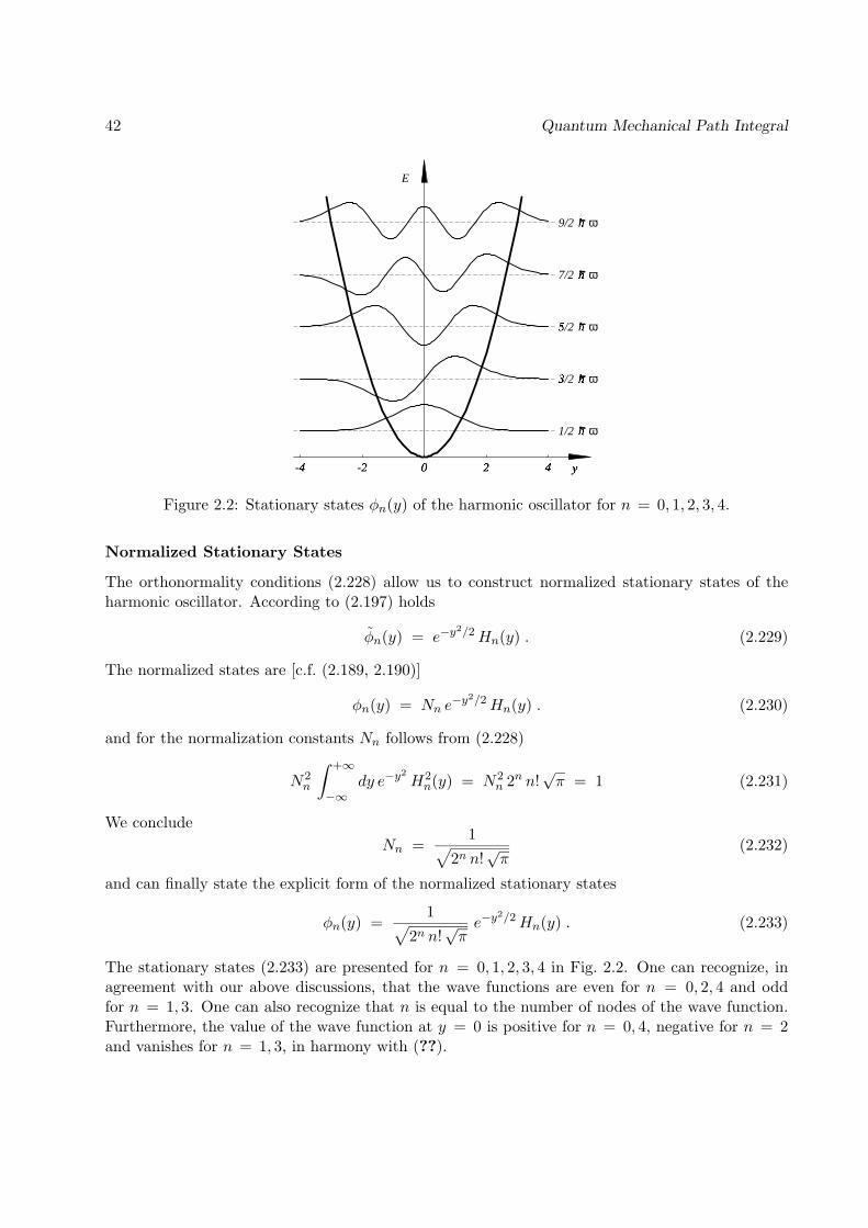
Figure 2.2: Stationary states φn(y) of the harmonic oscillator for n = 0, 1, 2, 3, 4.
Normalized Stationary States
The orthonormality conditions (2.228) allow us to construct normalized stationary states of theharmonic oscillator. According to (2.197) holds
φn(y) = e−y2/2Hn(y) . (2.229)
The normalized states are [c.f. (2.189, 2.190)]
φn(y) = Nn e−y2/2Hn(y) . (2.230)
and for the normalization constants Nn follows from (2.228)
N2n
∫ +∞
−∞dy e−y
2H2n(y) = N2
n 2n n!√π = 1 (2.231)
We concludeNn =
1√2n n!
√π
(2.232)
and can finally state the explicit form of the normalized stationary states
φn(y) =1√
2n n!√πe−y
2/2Hn(y) . (2.233)
The stationary states (2.233) are presented for n = 0, 1, 2, 3, 4 in Fig. 2.2. One can recognize, inagreement with our above discussions, that the wave functions are even for n = 0, 2, 4 and oddfor n = 1, 3. One can also recognize that n is equal to the number of nodes of the wave function.Furthermore, the value of the wave function at y = 0 is positive for n = 0, 4, negative for n = 2and vanishes for n = 1, 3, in harmony with (??).

2.5: Propagator for a Quadratic Lagrangian 43
The normalization condition (2.231) of the wave functions differs from that postulated in (2.189)by the Jacobian dx/dy, i.e., by √∣∣∣∣dxdy
∣∣∣∣ =[mω~
] 14. (2.234)
The explicit form of the stationary states of the harmonic oscillator in terms of the position variablex is then, using (2.233) and (2.189)
φn(x) =1√
2n n!
[mωπ~
] 14e−
mωx2
2~ Hn(√mω
~
x) . (2.235)
Completeness of the Hermite Polynomials
The Hermite polynomials are the first members of a large class of special functions which oneencounters in the course of describing stationary quantum states for various potentials and in spacesof different dimensions. The Hermite polynomials are so-called orthonogal polynomials since theyobey the conditions (2.228). The various orthonogal polynomials differ in the spaces Ω ⊂ R overwhich they are defined and differ in a weight function w(y) which enter in their orthonogalityconditions. The latter are written for polynomials pn(x) in the general form∫
Ωdx pn(x) pm(x) w(x) = In δnm (2.236)
where w(x) is a so-called weight function with the property
w(x) ≥ 0, w(x) = 0 only at a discrete set of points xk ∈ Ω (2.237)
and where In denotes some constants. Comparision with (2.228) shows that the orthonogalitycondition of the Hermite polynomials is in complience with (2.236 , 2.237) for Ω = R, w(x) =exp(−x2), and In = 2nn!
√π.
Other examples of orthogonal polynomials are the Legendre and Jacobi polynomials which arisein solving three-dimensional stationary Schrodinger equations, the ultra-spherical harmonics whicharise in n–dimensional Schrodinger equations and the associated Laguerre polynomials which arisefor the stationary quantum states of particles moving in a Coulomb potential. In case of theLegendre polynomials, denoted by P`(x) and introduced in Sect. 5 below [c.f. (5.150 , 5.151, 5.156,5.179] holds Ω = [−1, 1], w(x) ≡ 1, and I` = 2/(2` + 1). In case of the associated Laguerre
polynomials, denoted by L(α)n (x) and encountered in case of the stationary states of the non-
relativistic [see Sect. ??? and eq. ???] and relativistic [see Sect. 10.10 and eq. (10.459] hydrogenatom, holds Ω = [0,+∞[, w(x) = xαe−x, In = Γ(n+α+1)/n! where Γ(z) is the so-called Gammafunction.The orthogonal polynomials pn mentioned above have the important property that they form acomplete basis in the space F of normalizable functions, i.e., of functions which obey∫
Ωdx f2(x) w(x) = <∞ , (2.238)
where the space is endowed with the scalar product
(f |g) =∫
Ωdx f(x) g(x) w(x) = <∞ , f, g ∈ F . (2.239)
44 Quantum Mechanical Path Integral
As a result holds for any f ∈ Ff(x) =
∑n
cn pn(x) (2.240)
wherecn =
1In
∫Ωdx w(x) f(x) pn(x) . (2.241)
The latter identity follows from (2.236). If one replaces for all f ∈ F : f(x) →√w(x) f(x) and,
in particular, pn(x) →√w(x) pn(x) the scalar product (2.239) becomes the conventional scalar
product of quantum mechanics
〈f |g〉 =∫
Ωdx f(x) g(x) . (2.242)
Let us assume now the case of a function space governed by the norm (2.242) and the existence of anormalizable state ψ(y, t) which is stationary under the action of the harmonic oscillator propagator(2.147), i.e., a state for which (2.172) holds. Since the Hermite polynomials form a complete basisfor such states we can expand
ψ(y, t) =∞∑n=0
cn(t) e−y2/2Hn(y) . (2.243)
To be consistent with(2.188, 2.197) it must hold cn(t) = dn exp[−iω(n + 12)t] and, hence, the
stationary state ψ(y, t) is
ψ(y, t) =∞∑n=0
dn exp[−iω(n+12
)t] e−y2/2Hn(y) . (2.244)
For the state to be stationary |ψ(x, t)|2, i.e.,
∞∑n,m=0
d∗ndm exp[iω(m− n)t] e−y2Hn(y)Hm(y) , (2.245)
must be time-independent. The only possibility for this to be true is dn = 0, except for a singlen = no, i.e., ψ(y, t) must be identical to one of the stationary states (2.233). Therefore, the states(2.233) exhaust all stationary states of the harmonic oscillator.
Appendix: Exponential Integral
We want to prove
I =
+∞∫−∞
dy1 . . .
+∞∫−∞
dyn ei∑nj,k yjajkyk =
√(iπ)n
det(a), (2.246)
for det(a) 6= 0 and real, symmetric a, i.e. aT = a. In case of n = 1 this reads∫ +∞
−∞dx ei a x
2=
√i π
a, (2.247)

2.7: Appendix / Exponential Integral 45
which holds for a ∈ C as long as a 6= 0.The proof of (2.246) exploits that for any real, symmetric matrix exists a similarity transformationsuch that
S−1a S = a =
a11 0 . . . 00 a22 . . . 0...
.... . .
...0 0 . . . ann
. (2.248)
where S can be chosen as an orthonormal transformation, i.e.,
STS = 11 or S = S−1 . (2.249)
The akk are the eigenvalues of a and are real. This property allows one to simplify the bilinearform
∑nj,k yjajkyk by introducing new integration variables
yj =n∑k
(S−1)jkyk ; yk =n∑k
Skj yj . (2.250)
The bilinear form in (2.246) reads then in terms of yj
∑nj,k yjajkyk =
n∑j,k
n∑`m
y`Sj`ajkSkmym
=n∑j,k
n∑`m
y`(ST )`jajkSkmym
=n∑j,k
yj ajkyk (2.251)
where, according to (2.248, 2.249)
ajk =n∑l,m
(ST )jlalmSmk . (2.252)
For the determinant of a holds
det(a) =n∏j=1
ajj (2.253)
as well as
det(a) = det(S−1aS) = det(S−1) det(a) , det(S)= (det(S))−1 det(a) det(S) = det(a) . (2.254)
One can conclude
det(a) =n∏j=1
ajj . (2.255)

46 Quantum Mechanical Path Integral
We have assumed det(a) 6= 0. Accordingly, holds
n∏j=1
ajj 6= 0 (2.256)
such that none of the eigenvalues of a vanishes, i.e.,
ajj 6= 0 , for j = 1, 2, . . . , n (2.257)
Substitution of the integration variables (2.250) allows one to express (2.250)
I =
+∞∫−∞
dy1 . . .
+∞∫−∞
dyn
∣∣∣∣det(∂(y1, . . . , yn)∂(y1, . . . , yn)
)∣∣∣∣ ei∑nk akky
2k . (2.258)
where we introduced the Jacobian matrix
J =∂(y1, . . . , yn)∂(y1, . . . , yn)
(2.259)
with elementsJjs =
∂yj∂ys
. (2.260)
According to (2.250) holdsJ = S (2.261)
and, hence,
det(∂(y1, . . . , yn)∂(y1, . . . , yn)
) = det(S) . (2.262)
From (2.249) follows1 = det
(STS
)= ( det S )2 (2.263)
such that one can concludedet S = ±1 (2.264)
One can right then (2.258)
I =
+∞∫−∞
dy1 . . .
+∞∫−∞
dyn ei∑nk akky
2k
=
+∞∫−∞
dy1 eia11y2
1 . . .
+∞∫−∞
dyn eianny2
n =n∏k=1
+∞∫−∞
dyk eiakky
2k (2.265)
which leaves us to determine integrals of the type
+∞∫−∞
dx eicx2
(2.266)

2.7: Appendix / Exponential Integral 47
where, according to (2.257) holds c 6= 0.We consider first the case c > 0 and discuss the case c < 0 further below. One can relate inte-gral (2.266) to the well-known Gaussian integral
+∞∫−∞
dx e−cx2
=√π
c, c > 0 . (2.267)
by considering the contour integral
J =∮γ
dz eicz2
= 0 (2.268)
along the path γ = γ1 +γ2 +γ3 +γ4 displayed in Figure 2.3. The contour integral (2.268) vanishes,since eicz
2is a holomorphic function, i.e., the integrand does not exhibit any singularities anywhere
in C. The contour intergral (2.268) can be written as the sum of the following path integrals
J = J1 + J2 + J3 + J4 ; Jk =∮γk
dz eicz2
(2.269)
The contributions Jk can be expressed through integrals along a real coordinate axis by realizingthat the paths γk can be parametrized by real coordinates x
γ1 : z = x J1 =p∫−pdx eicx
2
γ2 : z = ix+ p J2 =p∫0
i dx eic(ix+p)2
γ3 : z =√i x J3 =
−√
2p∫√
2p
√i dx eic(
√ix)2
= −√i
√2p∫
−√
2p
dx e−cx2
γ4 : z = ix− p J4 =0∫−pi dx eic(ix−p)
2,
for x, p ∈ IR.
(2.270)
Substituting −x for x into integral J4 one obtains
J4 =
0∫p
(−i) dx eic(−ix+p)2
=
p∫0
i dx eic(ix−p)2
= J2 . (2.271)

48 Quantum Mechanical Path Integral
p
Im(z)
Re(z)
-p γ 1
γ 2
γ 3
γ 4
i p
-i p
Figure 2.3: Contour path γ in the complex plain.
We will now show that the two integrals J2 and J4 vanish for p → +∞. This follows from thefollowing calculation
limp→+∞
|J2 or 4| = limp→+∞
|p∫
0
i dx eic(ix+p)2 |
≤ limp→+∞
p∫0
|i| dx |eic(p2−x2)| |e−2cxp| . (2.272)
It holds |eic(p2−x2)| = 1 since the exponent of e is purely imaginary. Hence,
limp→+∞
|J2 or 4| ≤ limp→+∞
p∫0
dx |e−2cxp|
= limp→+∞
1− e−2cp
2 c p= 0 . (2.273)
J2 and J4 do not contribute then to integral (2.268) for p = +∞. One can state accordingly
J =
∞∫−∞
dx eicx2 −
√i
∞∫−∞
dx e−cx2
= 0 . (2.274)
Using 2.267) one has shown then∞∫−∞
dx eicx2
=
√iπ
c. (2.275)
2.7: Appendix / Exponential Integral 49
One can derive the same result for c < 0, if one chooses the same contour integral as (2.268), butwith a path γ that is reflected at the real axis. This leads to
J =
∞∫−∞
dx eicx2
+√−i
−∞∫∞
dx ecx2
= 0 (2.276)
and (c < 0)∞∫−∞
dx eicx2
=
√−iπ−|c|
=
√iπ
c. (2.277)
We apply the above results (2.275, 2.277) to (2.265). It holds
I =n∏k=1
√iπ
akk=
√(iπ)n∏nj=1 ajj
. (2.278)
Noting (2.255) this result can be expressed in terms of the matrix a
I =
√(iπ)n
det(a)(2.279)
which concludes our proof.

50 Quantum Mechanical Path Integral