Quantum Hall Effects

João Carlos de Andrade Getelina(Dated: November 23, 2018)

In this work we review the basic notions of quantum Hall effects. We present some of the theo-retical approaches developed to investigate the integer and fractional quantum Hall effects (IQHEand FQHE, respectively). For the integer quantum Hall effect we focus on the determination of thequantized transverse conductance via gauge invariance arguments. Conversely, for the fractionalquantum, we consider the variational method, which is based in introducing a trial wavefunction.We show that, in the thermodynamic limit, this trial wavefunction is related to a classical plasmain two dimensions, thus giving the relation for the quantization of the transverse conductance.

CONTENTS

I. Introduction 2

II. Background 2II.1. The experimental setup 2II.2. Landau levels 4II.3. The role of disorder 6

III. Integer quantum Hall effect 8

IV. Fractional quantum Hall effect 9

V. Concluding remarks 11

References 12

2

I. INTRODUCTION

It is no longer a surprise that, in the microscopic level, the properties of a system become quantized. However, anexperiment performed back in 1980 by von Klitzing et al. [1] showed a rather astonishing result: There are systemwhich exhibit quantized macroscopic properties. This experiment consisted of a two-dimensional free electrons systemunder strong magnetic fields and low temperatures. It was observed a quite unusual behavior of the conductance withrespect to the intensity of the magnetic field, consisting of relatively large steps of approximately constant conductancevalue. This phenomenon is now known as the quantum Hall effect (QHE), and it is believed to be one of the mostimportant achievements of condensed matter physics in the past century.

Since its first discovery, much progress has been made in the area of QHE. There are now many known types ofquantum Hall effects, but in particular we highlight the original ones, namely the integer quantum Hall effect (IQHE)and the fractional quantum Hall effect (FQHE). In the original paper by von Klitzing, it was observed the integerversion. Only two years later, the FQHE was observed by Tsui et al. [2]. There are several important distinctionsbetween these two effects, but the most basic one is that the conductance plateaus for the IQHE occur only at integervalues of the ratio e2/h, while for the FQHE these Hall conductance plateaus occur in rational values.

As one might guess, the QHE problem is a rather difficult one to solve: generally speaking, it involves a many-bodyinteracting system in the presence of a disordered potential. Over the years much effort has been made in order to geta good theoretical description of the system. Even though we are still far from the ultimate microscopic theory, thereare many theoretical approaches capable of encompassing various interesting physical properties. In a more technicalsense, one of the major contributions of QHE was the establishment of a reliable standard for conductance/resistance.The reason is that the integer of rational values of the conductance plateaus are measured with a precision of aboutone part in 1010, a rather remarkable figure.

The experimental observation of QHE has also paved the way to one of the most prolific areas in condensedmatter physics nowadays, which is the topological phases of matter. The relation between topology and QHE is thatthe observed phases cannot be described by a local order parameter; these QHE phases present what is known astopological order. Furthermore, in a more speculative manner, there is also great interested around topological phasesof matter directed to the application in quantum computing. Measurements of entanglement in those systems haveshown no decoherence effects, a quite desirable feature for a quantum computer.

This remaining of this paper is organized as follows. In Sec. II we present the general experimental setup, anddiscuss some basic concepts needed to understand the quantum Hall problem, such as the Landau levels and the roleof disorder. Sec. III is devoted to the IQHE, where we consider the gauge transformation approach [3, 4] in order todetermine the quantized conductance analytically. The FQHE is presented and discussed in Sec. IV, where we givethe general concepts of the variational method [5, 6]. Finally, in Sec. V we make an overview of the quantum Hallproblem and we provide a discussion about what improvements are yet to be achieved.

II. BACKGROUND

In this section we introduce the basic concepts related to the quantum Hall effect. We start by introducing thegeneral experimental setup, and we present the materials in which two-dimensional electron systems are realized. Inaddition, using classical electrodynamics theory, we compute the transverse conductance σxy, in order to compare tothe experimental observations. Next, we investigate the Hamiltonian of a single carrier under an external magneticfield, and obtain the corresponding eigenvalues and eigenstates, which are known as the Landau levels. Finally, wediscuss about the role of disorder in the quantum Hall effect, addressing the relation between random potentials andthe existence of plateaus of conductance.

II.1. The experimental setup

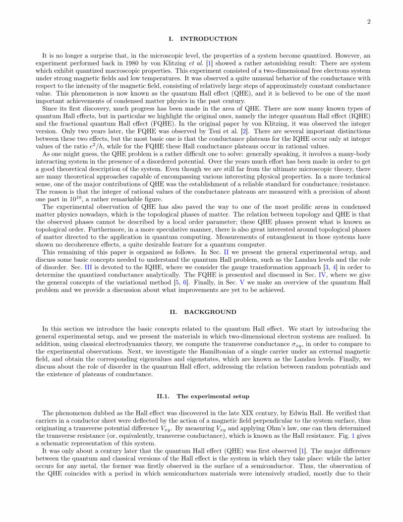
The phenomenon dubbed as the Hall effect was discovered in the late XIX century, by Edwin Hall. He verified thatcarriers in a conductor sheet were deflected by the action of a magnetic field perpendicular to the system surface, thusoriginating a transverse potential difference Vxy. By measuring Vxy and applying Ohm’s law, one can then determinedthe transverse resistance (or, equivalently, transverse conductance), which is known as the Hall resistance. Fig. 1 givesa schematic representation of this system.

It was only about a century later that the quantum Hall effect (QHE) was first observed [1]. The major differencebetween the quantum and classical versions of the Hall effect is the system in which they take place: while the latteroccurs for any metal, the former was firstly observed in the surface of a semiconductor. Thus, the observation ofthe QHE coincides with a period in which semiconductors materials were intensively studied, mostly due to their

3

Vxx

VxyE

J

B

Figure 1. General experimental setup for Hall effects.

(a) (b)

Si

EF

Valence band

Conduction bandMetal

SiO

2

VG

z

E

EF

VG

VG

Inversionlayer

z

E

Figure 2. Schematic of a Si MOSFET for the cases (a) VG = 0 and (b) VG > 0. Adapted from Ref. [9].

technological applications. Another significant difference between the classical and quantum Hall effects is that thelatter also requires stronger magnetic fields and much lower temperatures than the former.

The QHE was first observed in a Si MOSFET, i.e., a silicon metal-oxide-semiconductor field-effect transistor. Inthis system, a layer of SiO2, which is an insulator, separates a layer of silicon doped with acceptors and a metal.There is also a potential difference VG between the semiconductor and the metal, as shown in Fig. 2. The role of VGis to induce an electric field between the surface of the metal and the semiconductor, such as in a capacitor. As weincrease VG, the corresponding electric field bends the energy levels of the semiconductor, up to the point where theconduction band gets below the Fermi level, as shown in Fig. 2. In this case, the electrons near the semiconductorsurface are able to occupy the conduction band, thus being able to move freely in the xy plane. This thin layer closeto the semiconductor surface is known as the inversion layer. Notice that the electron density of the inversion layer,which is usually set about 1015–1017m−2 , can be controlled by the gate potential VG.

An important property of the Si MOSFET to note is the existence of charged acceptors within or close to theinversion layer, as shown in Fig. 2. These atoms act as impurities, which generate a position-dependent randompotential for the electrons in the conduction band. As we shall see, this random potential plays a major role in theunderstanding of the integer quantum Hall effect. There are systems in which the effect of the random potentialcan be better controlled, such as in GaAs-AlGaAs heterojuctions. In these systems, it has been observed both theinteger [7] and fractional [2] Hall effects. For our purposes, it suffices to discuss the properties of the Si MOSFET; thereader interested in other heterojunctions may look at Refs. [8, 9]. In addition, it is important to emphasize that theQHE is not restricted to semiconductor heterojuctions; recently, for example, it has been verified QHE in grapheneat room temperature [10].

Since we have already established the general experimental setup, as depicted in Fig. 1, we can now make predictionsabout the behavior of the transverse conductance σxy. For instance, according to classical electrodynamics, the steady-state solution is given by equating the forces due to the electric and magnetic fields, i.e.,

eE = −ev ×B, (1)

which gives us the following drift velocity:

v = −EB. (2)

Notice that the drift velocity is perpendicular to the electric field. Thus, the particle travels in equipotential lines. In

4

ne/B

σxy T = 0

classicalexperiment

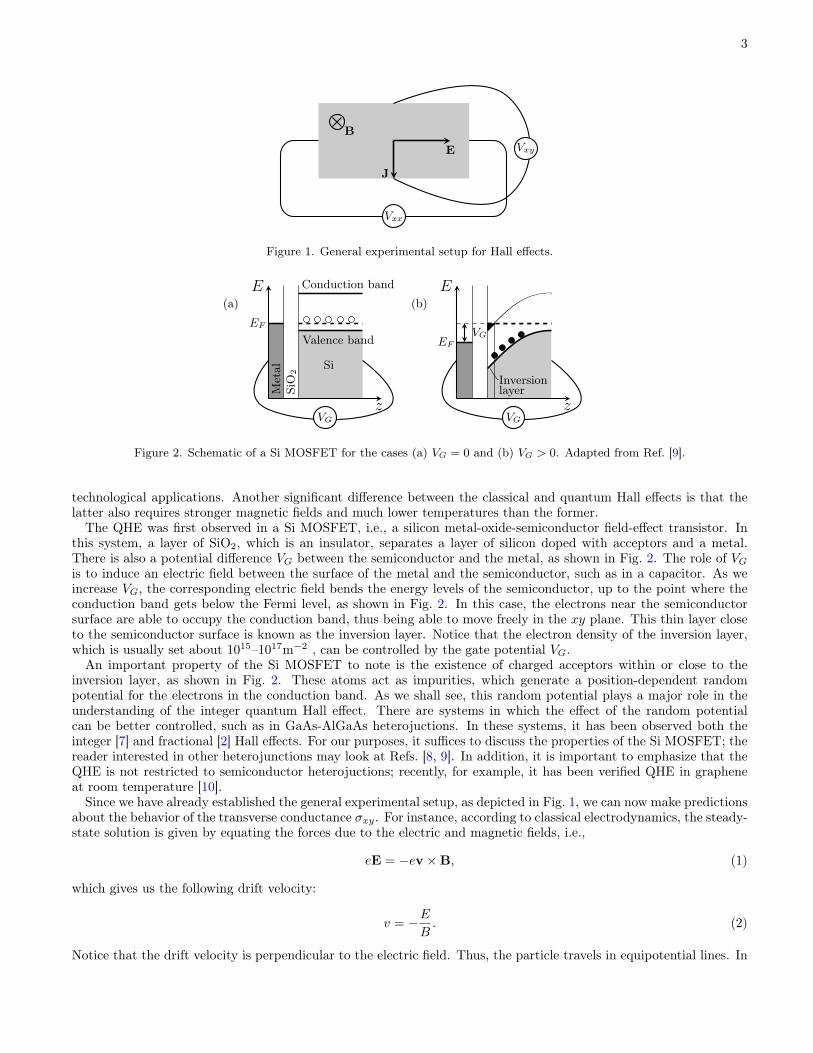
Figure 3. Sketch of the transverse conductance σxy accordingly to the classical prediction and the experimental observation,at zero temperature.

addition, the current density J is given by

J = −nev, (3)

where n is the electron density. The connection between the current density and the electric field is given by theconductivity tensor σ, i.e., J = σE. Thus, substituting the drift velocity in the previous equation, we find anexpression for the transverse conductance σxy:

σxy =ne

B. (4)

(Similarly, the longitudinal conductance is σxx = 0.) Hence, according to classical electrodynamics, the transverseconductance increases linearly with the ratio n/B.

However, under strong magnetic fields and low temperatures, the picture observed experimentally is quite differentfrom the classical prediction, as illustrated in Fig. 3. As aforementioned, the experiment exhibits plateaus of transverseconductance, which are given by the following expression

σxy =e2

2π~ν, (5)

where ν ∈ N. The integer value ν, which is known as the filling factor, is measured with a rather astonishing precision:in the order of one part in 1010 for some filling factors close to the center of its plateau. Thanks to this precision, theHall resistance ρxy = 1/σxy became the standard value of resistance. Finally, the simple appearance of ~ in Eq. (5)tells us that we need a quantum treatment of the problem to obtain the correct behavior of the Hall conductance, aswe address in the following.

II.2. Landau levels

Let us consider a single electron of charge −e, confined to the xy plane, under the presence of an external magneticfield B = −Bz. The Hamiltonian of this system is given by

H0 =1

2m(p + eA)

2=

1

2mπ2. (6)

The gauge choice in problems containing the vector field A is very important, since a wise choice may simplify theproblem considerably. In QHE systems, there are two gauge choices that proved to be useful, namely the Landaugauge and the symmetric gauge. The Landau gauge is especially suited for problems in a rectangular geometry. It isgiven by the following relation:

A = −xBy. (7)

On the other hand, the symmetric gauge is defined as

A =B

2(yx− xy) . (8)

This gauge is useful for problems with rotational symmetry.

5

However, there is a faster way of obtaining the energy spectrum of (6) without referring to any gauge. First, noticethat the commutator between the components of π is given by

[πx, πy] = −i~2

l20, (9)

where l0 =√

~/eB is the magnetic length. Therefore, by a proper normalization, the two components of π give apair of canonical operators. Since the Hamiltonian is a sum of the squares of canonical operators, we may proceed asin the harmonic oscillator, where we introduce the dimensionless creation/annihilation operators:

a† =1

~√

2(πx + iπy) , a =

1

~√

2(πx − iπy) , (10)

Hence, the Hamiltonian is rewritten as

H0 = ~ωc(a†a+

1

2

), (11)

where ωc = eB/m is the cyclotron frequency, and, consequently the eigenvalues are given by

En = ~ωc(n+

1

2

), n = 0, 1, . . . (12)

The corresponding eigenstates are known as the Landau levels. Throughout this work we are going to be interestedin calculating the system low-lying excitations. Thus, the lowest Landau level (LLL), i.e., the state with n = 0 willbe constantly referred to.

The whole physics of the problem has not yet been captured. For instance, one would expect the electron tobe described by two quantum numbers, since it is restricted to move in the xy plane. To find this extra quantumnumber, we will have to choose a gauge. As we shall see in the following, the second quantum number expresses theenormous degeneracy contained in each Landau level. To observe this huge degeneracy without explicitly determiningthe eigenstates, let us consider the following operator:

R = Xx+ Y x = r− l20~z × π. (13)

The components of this operator also yield a canonical commutation relation, where ~ is replace by l20. Thus, we mayemploy the Bohr-Sommerfeld quantization rule, in which the area of the phase space is proportional to h. Here, thearea of the phase space corresponds to the area of the sample itself, which is given by LxLy. Therefore, the degeneracyD of each Landau level is given by

D =LxLy2πl20

=LxLyeB

2π~=

1

Φ0LxLyB =

Φ

Φ0, (14)

where Φ0 = 2π~/e is the flux quanta. This enormous degeneracy forbids us to employ perturbation theory in orderto include the interactions and impurities in Hamiltonian.

Diving D by the number of particles N we get the number of available states per particle, i.e.,

D

N=LxLyN

eB

2π~=

eB

2πn~. (15)

Note that the right-hand side of the expression above is obtained if we equate Eqs. (4) and (5), which corresponds tothe points where the classical prediction intercepts the experimental result. Thus, we get the following relation

D

N=

1

ν. (16)

This expression is useful to interpret the fractional quantum Hall effect; for instance, the filling factor ν = 1/3 tells usthat there are three available states per particle at the LLL. On the other hand, for the integer quantum Hall effect,ν gives us the number of filled Landau levels.

To determine the eigenstates of (6) we will consider both the Landau and the symmetric gauge, Eqs. (7) and (8),respectively. As we shall verify in the next sections, the former is more adequate to the IQHE, while the latter is usedto describe the FQHE. Let us consider first the Landau gauge. Substituting Eq. (7) in (6) we find

H0 =1

2m

[p2x + (py − eBx)

2]. (17)

6

Note that the expression above is translationally invariant in the y-direction. Thus, one may look for solutions as thefollowing:

ψk (x, y) = f (x) eiky. (18)

Using this Ansatz, one may find that the Hamiltonian corresponds to a harmonic oscillator with the center displacedby −kl20. Hence, the complete eigenfunctions (ignoring the normalization) are given by

ψn,k (x, y) = eikyHn (x) e−(x−kl20)2/2l20 , (19)

where Hn (x) are the Hermite polynomials.Conversely, by inserting the symmetric gauge (8) in (6) we find

H0 =1

2m

[(px +

B

2y

)2

+

(py −

B

2x

)2]. (20)

This Hamiltonian commutes with the z-component of the angular momentum, thus we may use the eigenvalue of Lzas a quantum number. In addition, notice that Lz may be written in terms of the two pairs of canonical operators,namely π and R:

Lz = − ~2l20

(X2 + Y 2

)+l202~(π2x + π2

y

). (21)

Hence, we can introduce new creation/annihilation operators, b and b† respectively, which are related to R, similarlyto Eq. (10). Thus, we obtain

Lz = ~(a†a− b†b

), (22)

with a general eigenstate given by

|n,m〉 =

(a†)n (

b†)m

√n!√m!

|0, 0〉 . (23)

Here, the quantum number n gives the energy, while m gives the degeneracy. To obtain the eigenstates (23) in thecoordinate representation, it is convenient to introduce complex variables z = x + iy. For the lowest Landau level(LLL), we have the condition a |LLL〉 = 0, which gives (ignoring the normalization)

ψLLL (z) = zme−|z|2/4l20 , m = 0, 1, 2, . . . (24)

This eigenfunction will be frequently used in the investigation of the FQHE.Finally, notice that throughout this discussion, we have omitted the electric field. The reason is that the effect of

the electric field is equivalent to what we observed in the classical case; the superposition of the cyclotron motionand a constant drift velocity perpendicular to the electric field. Moreover, as a side note, one could argue about therole of the electron spin, since the magnetic field lifts up the spin degeneracy. It is reasonable to assume that, undersuch strong magnetic fields, the spins are all polarized, i.e., pointing in the same direction of the magnetic field. Inpractice, however, the electron spin does indeed play a role, especially in the case of some exotic filling factors in thefractional quantum Hall effect. Nevertheless, for the sake of simplicity, we disregard the electron spin throughout thiswork.

II.3. The role of disorder

Before providing an explicit calculation of the transverse conductance, we make a phenomenological discussion aboutthe existence of the Hall resistance plateaus, as depicted in Fig. 3. As we have discussed previously, the presenceof impurities affecting the inversion layer is inevitable. However, according to Anderson localization theory [11],any amount of disorder in a two-dimensional system at zero temperature makes every state localized. Thus, theobservation of a Hall current would be impossible, since transport only occurs for extended states in zero temperature.Nevertheless, the experiment shows that there is indeed a Hall current.

The explanation for this inconsistency between localization theory and the QHE experimental observation relies onthe complete disregard of the Hall conductance in the development of the one-parameter scaling theory of localization.

7

+

− y

x

E

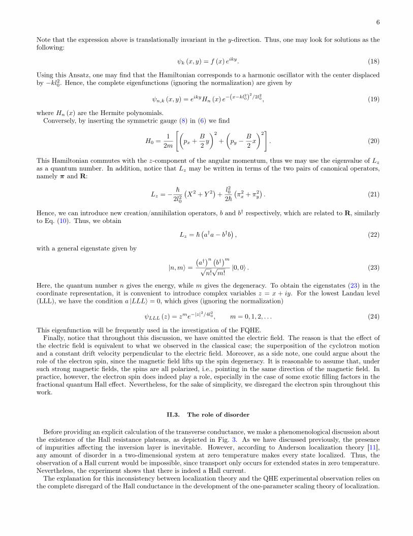
Figure 4. Bending of the equipotential lines caused by a random potential. Here, we are considering a region of the systemaway from the edges.

E12~ωc

32~ωc

ρ(E)

EF

localizedextended

Figure 5. Density of states ρ (E) of the electron in a magnetic field and in the presence of a random potential. EF denotes theFermi level. Adapted from Ref. [9].

However, there has been some efforts in order to include the Hall conductance, and hence the effect of magnetic fields,in the scaling theory of localization. First attempts considered a two-parameter scaling theory, which was ableto predict the basic features of conductance, and also a shift in the position of the extended states in the energyspectrum as disorder becomes comparable to the Landau levels gap [12]. Further improvements were achieved by athree-parameter scaling theory, which included the electron-electron interactions. This theory was able to predict aorder-disorder phase transition, corresponding to the destruction of the QHE [13].

To understand how disorder affects the properties of the system states, let us first consider the case free of ran-domness, in which the single-particle states are given by the Langau gauge eigenstates in (19). Notice that the thesestates are extended in the y-direction since they are described by a plane wave, and are thus able to contribute tothe Hall current. Now let us turn on the random potential caused by impurities. Suppose that this random potentialhave some local maxima and minima, as depicted in Fig. 4. Thus, the equipotential lines generated by the appliedelectric field are no longer longitudinal; the extreme points of the random potential will bend the equipotential lines,making a closed trajectory around them (see Fig. 4). Therefore, an electron which falls into one of these enclosedpotential lines becomes localized and thus cannot contribute to the Hall current.

One could argue, however, whether this localization mechanism induced by the random potential is able to localizedall the system states. From the experimental point of view, one knows that this is not possible since the Hall currentis indeed observed. On the other hand, as we shall see in the next section, from the theoretical point of view it isnecessary to assume that at least one of the system states remains extended in the presence of disorder [4]. It was laterverified from both numerical and analytical calculations that the system density of states in the presence of disorderis as follows: There is a small region of extended states near the eigenvalues of the Landau levels in the absenceof disorder. This small region is surrounded by localized states only, as depicted in Fig. 5. Therefore, according tothis picture, as we vary the Fermi level EF , either by changing the electrons density or the magnetic field, the Hallconductance remains constant since localized states do not contribute to the current; we only observe a change inthe transverse conductance as we reach the next extended state, which corresponds to the sharp steps in between theplateaus.

This configuration of the density of states, in which a small region of extended states is enclosed by localized ones,has been extensively verified via numerical methods. One can find delocalized states by observing the variation of the

8

Vxx

B

R

L

Φ + ∆Φ

y

x

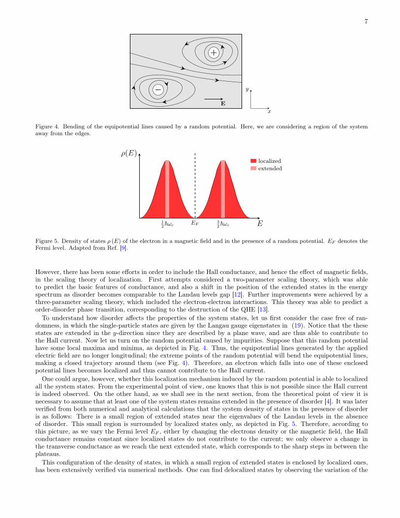
Figure 6. Transformed quantum Hall system as a cylinder of radius R and length L, with a flux Φ passing through the center.Adapted from Ref. [9].

localization length ξ with respect to the energy. Indeed, it has been observed that close to the Landau level energies,the localization length diverges as [14]

ξ ∝ |E − Ec|−ν , ν = 2.35± 0.08,

where Ec is the corresponding Landau level energy. This exponent has not yet been determined analytically.

III. INTEGER QUANTUM HALL EFFECT

To explain the conductance plateaus in the IQHE, Laughlin came up with a rather elegant argument, based solelyin properties of gauge invariance. Consider our QHE system on the surface of a cylinder of radius R and length L,as shown in Fig. 6. The y-direction surrounds the system surface while the x-direction is parallel to the cylinderaxis. Thus, the magnetic field B must be radial with respect to the cylinder axis. Even though this configurationis not useful for experimental purposes, since the periodic boundary condition in the y-direction does not allow formeasurements of the Hall conductance, it provides us a fast calculation of the quantization of σxy.

The key point to argument is to add a solenoid in the center of the cylinder, as depicted in Fig. 6. This solenoidgenerates a magnetic flux Φ, and, according to the Aharonov-Bohm effect, this flux induces a vector potential AΦ onthe system. From Stoke´s law, one may find that

Φ =

˛dl ·AΦ = 2πR |AΦ| . (25)

This change in the vector potential may be thought of as a gauge transformation.Consider now a flux variation ∆Φ in the solenoid. This induces a phase shift in the electron wavefunction, which

is given by

ψ (x, y)→ ψ (x, y) e−iey∆Φ/(hR). (26)

However, in the configuration we considered, the boundary conditions do not allow any gauge transformation to takeplace. We have to consider two possibilities: (i) the states in the surface are extended or (ii) the states in the surfaceare localized. For the latter case, any continuous gauge transformation is permitted. Conversely, for the case (i), thegauge transformation must respect a full phase shift, i.e, ψ (x, y + 2πR) = ψ (x, y), implying that

∆Φ =h

e× integer. (27)

Therefore, to obtain any relevant change to the system wavefunctions, we have to assume that the states areextended. We then look to the situation in which the flux variation does not respect the criterion (27). In this case,since the total vector potential is given by

A + AΦ = B

(x− Φ

2πRB

)y, (28)

9

a flux variation Φ → Φ + ∆Φ will only cause a shift in the x-direction. Hence, the electron extended states simplymove to the next one along the cylinder axis. Under the presence of disorder, some of the extended states will betransformed into localized ones. The latter are not able to move along the x-direction, regardless whether (27) issatisfied. On the other hand, the remaining extended states are still able to pass through these localized ones. Thus,it suffices to postulate that there is at least one extended state in the random system.

Now recall that in the IQHE, all extended states below the Fermi level are occupied. Thus, if we consider a fluxvariation ∆Φ = h/e, all electrons must move to the next extended states. However, at the end of the cylinder,the electron in the last extended state flows out of the system, which is then supplied with another electron by theelectrode. Hence, the number of electrons ν that flows in/out of the system corresponds to the number of Landaulevels below the Fermi level. The energy cost of this process is given by

∆E = eVxxN. (29)

We can relate this energy cost to the current density in the y-direction as follows:

Jy = − 1

2πRL

⟨∑i

e

m[piy + eAy (ri)]

⟩

=1

L

⟨∂

∂Φ

{∑i

1

2m

[p2ix + (piy + eAy)

2]

+ Vimp (ri)

}⟩

=1

L

⟨∂H

∂Φ

⟩=

1

L

∂

∂Φ〈E〉 . (30)

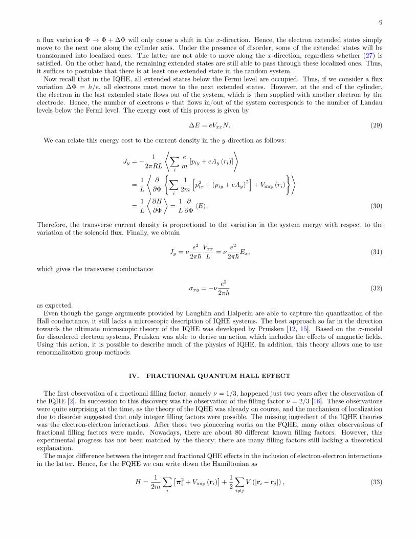
Therefore, the transverse current density is proportional to the variation in the system energy with respect to thevariation of the solenoid flux. Finally, we obtain

Jy = νe2

2π~VxxL

= νe2

2π~Ex, (31)

which gives the transverse conductance

σxy = −ν e2

2π~(32)

as expected.Even though the gauge arguments provided by Laughlin and Halperin are able to capture the quantization of the

Hall conductance, it still lacks a microscopic description of IQHE systems. The best approach so far in the directiontowards the ultimate microscopic theory of the IQHE was developed by Pruisken [12, 15]. Based on the σ-modelfor disordered electron systems, Pruisken was able to derive an action which includes the effects of magnetic fields.Using this action, it is possible to describe much of the physics of IQHE. In addition, this theory allows one to userenormalization group methods.

IV. FRACTIONAL QUANTUM HALL EFFECT

The first observation of a fractional filling factor, namely ν = 1/3, happened just two years after the observation ofthe IQHE [2]. In succession to this discovery was the observation of the filling factor ν = 2/3 [16]. These observationswere quite surprising at the time, as the theory of the IQHE was already on course, and the mechanism of localizationdue to disorder suggested that only integer filling factors were possible. The missing ingredient of the IQHE theorieswas the electron-electron interactions. After those two pioneering works on the FQHE, many other observations offractional filling factors were made. Nowadays, there are about 80 different known filling factors. However, thisexperimental progress has not been matched by the theory; there are many filling factors still lacking a theoreticalexplanation.

The major difference between the integer and fractional QHE effects in the inclusion of electron-electron interactionsin the latter. Hence, for the FQHE we can write down the Hamiltonian as

H =1

2m

∑i

[π2i + Vimp (ri)

]+

1

2

∑i 6=j

V (|ri − rj |) , (33)

10

where Vimp (r) is the random potential caused by the impurities, and V (|ri − rj |) stands for the electron-electroninteractions. The usual approach to face a problem such as in Eq. (33) is to assume the interaction term as a smallperturbation to the remaining terms, and employ perturbation theory. However, as we have discussed previously, themassive degeneracy of the Landau levels forbids us to even start a perturbative method.

The first alternative to the perturbative approach was developed by Laughlin [5]. The author had a great deal ofphysical insight of the problem, where he imagined that electrons in FQHE systems would like to stay as far fromeach other as possible. Hence, inspired by previous works on liquid helium, a system where the particles also preferto be far apart from each other, he proposed a trial wavefunction, which is the following:

ψ (zi) =∏i<j

(zi − zj)m exp

(−

N∑k=1

|zk|2

4l2B

), (34)

where m is an odd integer, in order to respect Pauli’s principle.Given this trial wavefunction, let us consider the expectation value of a general operator O (z). Hence, From the

definition, we have

〈O (z)〉 =

´ ∏i d

2ziO (z)P [zi]´ ∏i d

2ziP [zi], (35)

where the unnormalized probability distribution P [zi] is defined as

P [zi] =∏i<j

|zi − zj |2m

l2mBexp

(−

N∑k=1

|zk|2

4l2B

). (36)

The expectation value in (35) is very difficult to compute. However, notice that by writing P [zi] = e−βH(zi), andsetting β = 2/m, we find:

H (zi) =1

2βl2B

∑i

|zi|2 −2m

β

∑i<j

ln

(|zi − zj |lB

). (37)

The expression above corresponds to the energy of a classical one-component plasma of charged particles in two-dimensions. For instance, consider that this plasma is composed of particles with charge −σ, and a backgroundpotential density ρ. Hence, the corresponding potential energy is given by

U (zi) =ρσ

4ε

∑i

|zi|2 −σ2

2πε

∑i<j

ln

(|zi − zj |lB

), (38)

where ε is the dielectric constant. Thus, in the thermodynamic equilibrium, the particle density of the plasma isn = ρ/σ.

By comparing Eqs. (37) and (38), we find that

ρσ

4ε=

1

2βl20,

σ2

2πε=

2m

β, (39)

which gives

1

m= 2πl20n. (40)

Finally, according to Eqs. (15) and (16), we find that

ν =1

m. (41)

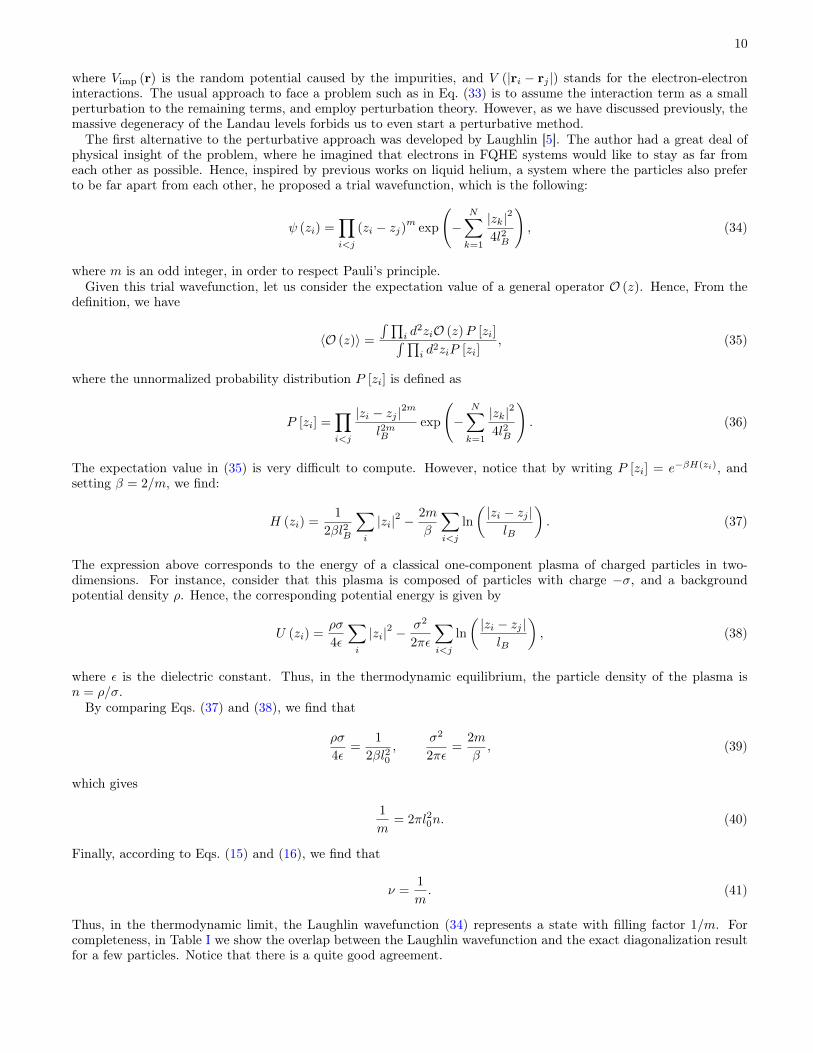
Thus, in the thermodynamic limit, the Laughlin wavefunction (34) represents a state with filling factor 1/m. Forcompleteness, in Table I we show the overlap between the Laughlin wavefunction and the exact diagonalization resultfor a few particles. Notice that there is a quite good agreement.

11

N Matrix dimension 〈ψ0| ψexact〉4 15 0.998045 73 0.999066 338 0.996447 1656 0.996368 8512 0.995409 45207 0.99406

Table I. Overlap between the Laughlin wavefunction and the exact ground state obtained numerically for the filling factorν = 1/3. Adapted from Ref. [17].

V. CONCLUDING REMARKS

In this work we have reviewed one of the most relevant discoveries of the past century in the area of condensedmatter physics, which is the quantum Hall effect. We have provided a general background for the problem whilediscussing the experimental setup, the single-particle eigenstates and the role of disorder. For the integer fillingfactors case, we have limited our discussion to the calculation of the transverse conductance from the gauge invariancearguments. Other important approaches have been neglected, such as those concerning the existence of edge states,and the field-theoretical approach [12, 15]. Conversely, for the fractional filling factor case, we considered the trialwavefunction developed by Laughlin, and compared the overlap between this theory and exact numerical calculations,which shows a good agreement for few electrons.

It is clear that the quantum Hall effect is still an open problem. For instance, in the case of the FQHE, thetheoretical approaches developed so far are not able to capture the physics of any observed filling factor. In addition,it has not yet been determined the critical filling factor upon which the Wigner crystal phase becomes energeticallymore favorable. Other important discrepancy between theory and experiment relies on the measurement of the energygap. States which are not incompressible fluids, such as the ones with even-denominator filling factor, are still notcompletely understood. Finally, as a guidance for further investigations, one could argue the investigation of strongmagnetic field effects in lower-dimensional systems, such as one-dimensional chains or quantum dots.

12

[1] K. v. Klitzing, G. Dorda, and M. Pepper, Phys. Rev. Lett. 45, 494 (1980).[2] D. C. Tsui, H. L. Stormer, and A. C. Gossard, Phys. Rev. Lett. 48, 1559 (1982).[3] R. B. Laughlin, Phys. Rev. B 23, 5632 (1981).[4] B. I. Halperin, Phys. Rev. B 25, 2185 (1982).[5] R. B. Laughlin, Phys. Rev. Lett. 50, 1395 (1983).[6] R. B. Laughlin, Phys. Rev. B 27, 3383 (1983).[7] M. A. Paalanen, D. C. Tsui, and A. C. Gossard, Phys. Rev. B 25, 5566 (1982).[8] R. E. Prange and S. M. Girvin, eds., The Quantum Hall Effect (Springer New York, 1990).[9] D. Yoshioka, The Quantum Hall Effect (Springer Berlin Heidelberg, 2002).

[10] K. S. Novoselov, Z. Jiang, Y. Zhang, S. V. Morozov, H. L. Stormer, U. Zeitler, J. C. Maan, G. S. Boebinger, P. Kim, andA. K. Geim, Science 315, 1379 (2007), http://science.sciencemag.org/content/315/5817/1379.full.pdf.

[11] E. Abrahams, P. W. Anderson, D. C. Licciardello, and T. V. Ramakrishnan, Phys. Rev. Lett. 42, 673 (1979).[12] A. M. M. Pruisken, Phys. Rev. B 32, 2636 (1985).[13] R. B. Laughlin, M. L. Cohen, J. M. Kosterlitz, H. Levine, S. B. Libby, and A. M. M. Pruisken, Phys. Rev. B 32, 1311

(1985).[14] B. Huckestein, Rev. Mod. Phys. 67, 357 (1995).[15] A. Pruisken, Nuclear Physics B 235, 277 (1984).[16] H. Stormer, D. Tsui, A. Gossard, and J. Hwang, Physica B+C 117-118, 688 (1983).[17] G. Fano, F. Ortolani, and E. Colombo, Phys. Rev. B 34, 2670 (1986).