quantum field theory -...
TRANSCRIPT


Quantum Field TheoryCompetitive Models
Bertfried FauserJürgen TolksdorfEberhard ZeidlerEditors
BirkhäuserBasel · Boston · Berlin
- -


CONTENTS
Preface . . . . . . . . . . . . . . . . . . . . . . . . . . . . . . . . . . . . . . . . . . . . . . . . . . . . . . . . . . . . . . . . . . . . . xiiiBertfried Fauser, Jurgen Tolksdorf and Eberhard Zeidler
Constructive Use of Holographic Projections . . . . . . . . . . . . . . . . . . . . . . . . . . . . . . . . 1Bert Schroer
1. Historical background and present motivations for holography . . . . . . . . 12. Lightfront holography, holography on null-surfaces and the origin
of the area law . . . . . . . . . . . . . . . . . . . . . . . . . . . . . . . . . . . . . . . . . . . . . . . . . . . . . . . 43. From holography to correspondence: the AdS/CFT correspondence
and a controversy . . . . . . . . . . . . . . . . . . . . . . . . . . . . . . . . . . . . . . . . . . . . . . . . . . . . 144. Concluding remarks . . . . . . . . . . . . . . . . . . . . . . . . . . . . . . . . . . . . . . . . . . . . . . . . . . 22Acknowledgements . . . . . . . . . . . . . . . . . . . . . . . . . . . . . . . . . . . . . . . . . . . . . . . . . . . . . . . 23References. . . . . . . . . . . . . . . . . . . . . . . . . . . . . . . . . . . . . . . . . . . . . . . . . . . . . . . . . . . . . . . . 23
Topos Theory and ‘Neo-Realist’ Quantum Theory . . . . . . . . . . . . . . . . . . . . . . . . . . . 25Andreas Doring
1. Introduction . . . . . . . . . . . . . . . . . . . . . . . . . . . . . . . . . . . . . . . . . . . . . . . . . . . . . . . . . 251.1. What is a topos? . . . . . . . . . . . . . . . . . . . . . . . . . . . . . . . . . . . . . . . . . . . . . . . 261.2. Topos theory and physics . . . . . . . . . . . . . . . . . . . . . . . . . . . . . . . . . . . . . . . 29
2. A formal language for physics . . . . . . . . . . . . . . . . . . . . . . . . . . . . . . . . . . . . . . . . 313. The context category V(R) and the topos of presheaves SetV(R)op
. . . 334. Representing L(S) in the presheaf topos SetV(R)op
. . . . . . . . . . . . . . . . . . 355. Truth objects and truth-values . . . . . . . . . . . . . . . . . . . . . . . . . . . . . . . . . . . . . . . 38
5.1. Generalized elements as generalized states . . . . . . . . . . . . . . . . . . . . . . 385.2. The construction of truth objects . . . . . . . . . . . . . . . . . . . . . . . . . . . . . . . 395.3. Truth objects and Birkhoff-von Neumann quantum logic . . . . . . . . 415.4. The assignment of truth-values to propositions. . . . . . . . . . . . . . . . . . 42
6. Conclusion and outlook . . . . . . . . . . . . . . . . . . . . . . . . . . . . . . . . . . . . . . . . . . . . . . 45Acknowledgements . . . . . . . . . . . . . . . . . . . . . . . . . . . . . . . . . . . . . . . . . . . . . . . . . . . . . . . 45References. . . . . . . . . . . . . . . . . . . . . . . . . . . . . . . . . . . . . . . . . . . . . . . . . . . . . . . . . . . . . . . . 46
A Survey on Mathematical Feynman Path Integrals:Construction, Asymptotics, Applications . . . . . . . . . . . . . . . . . . . . . . . . . . . . . . . . . . . . 49Sergio Albeverio and Sonia Mazzucchi
1. Introduction . . . . . . . . . . . . . . . . . . . . . . . . . . . . . . . . . . . . . . . . . . . . . . . . . . . . . . . . . 492. The mathematical realization of Feynman path integrals . . . . . . . . . . . . . . 523. Applications . . . . . . . . . . . . . . . . . . . . . . . . . . . . . . . . . . . . . . . . . . . . . . . . . . . . . . . . . 56
3.1. Quantum mechanics . . . . . . . . . . . . . . . . . . . . . . . . . . . . . . . . . . . . . . . . . . . . 56
vi
3.2. Quantum fields . . . . . . . . . . . . . . . . . . . . . . . . . . . . . . . . . . . . . . . . . . . . . . . . . 60Acknowledgements . . . . . . . . . . . . . . . . . . . . . . . . . . . . . . . . . . . . . . . . . . . . . . . . . . . . . . . 62References. . . . . . . . . . . . . . . . . . . . . . . . . . . . . . . . . . . . . . . . . . . . . . . . . . . . . . . . . . . . . . . . 62
A Comment on the Infra-Red Problem in the AdS/CFT Correspondence . . . 67Hanno Gottschalk and Horst Thaler
1. Introduction . . . . . . . . . . . . . . . . . . . . . . . . . . . . . . . . . . . . . . . . . . . . . . . . . . . . . . . . . 672. Functional integrals on AdS . . . . . . . . . . . . . . . . . . . . . . . . . . . . . . . . . . . . . . . . . . 683. Two generating functionals . . . . . . . . . . . . . . . . . . . . . . . . . . . . . . . . . . . . . . . . . . . 714. The infra-red problem and triviality . . . . . . . . . . . . . . . . . . . . . . . . . . . . . . . . . . 755. Conclusions and outlook. . . . . . . . . . . . . . . . . . . . . . . . . . . . . . . . . . . . . . . . . . . . . . 79Acknowledgement . . . . . . . . . . . . . . . . . . . . . . . . . . . . . . . . . . . . . . . . . . . . . . . . . . . . . . . . 80References. . . . . . . . . . . . . . . . . . . . . . . . . . . . . . . . . . . . . . . . . . . . . . . . . . . . . . . . . . . . . . . . 80
Some Steps Towards Noncommutative Mirror Symmetry on the Torus . . . . . . 83Karl-Georg Schlesinger
1. Introduction . . . . . . . . . . . . . . . . . . . . . . . . . . . . . . . . . . . . . . . . . . . . . . . . . . . . . . . . . 832. Elliptic curves . . . . . . . . . . . . . . . . . . . . . . . . . . . . . . . . . . . . . . . . . . . . . . . . . . . . . . . . 843. Noncommutative elliptic curves . . . . . . . . . . . . . . . . . . . . . . . . . . . . . . . . . . . . . . . 854. Exotic deformations of the Fukaya category. . . . . . . . . . . . . . . . . . . . . . . . . . . 885. Conclusion and outlook . . . . . . . . . . . . . . . . . . . . . . . . . . . . . . . . . . . . . . . . . . . . . . 91Acknowledgements . . . . . . . . . . . . . . . . . . . . . . . . . . . . . . . . . . . . . . . . . . . . . . . . . . . . . . . 92References. . . . . . . . . . . . . . . . . . . . . . . . . . . . . . . . . . . . . . . . . . . . . . . . . . . . . . . . . . . . . . . . 92
Witten’s Volume Formula, Cohomological Pairings of Moduli Spaces ofFlat Connections and Applications of Multiple Zeta Functions . . . . . . . . . . . . . . . 95Partha Guha
1. Introduction . . . . . . . . . . . . . . . . . . . . . . . . . . . . . . . . . . . . . . . . . . . . . . . . . . . . . . . . . 952. Background about moduli space . . . . . . . . . . . . . . . . . . . . . . . . . . . . . . . . . . . . . . 1013. Volume of the moduli space of SU(2) flat connections . . . . . . . . . . . . . . . . 103
3.1. Asymptotic analysis and computation of volumeof moduli spaces . . . . . . . . . . . . . . . . . . . . . . . . . . . . . . . . . . . . . . . . . . . . . . . . 104
4. Volume of the moduli space of flat SU(3) connections . . . . . . . . . . . . . . . . 1065. Cohomological pairings of the moduli space. . . . . . . . . . . . . . . . . . . . . . . . . . . 108
5.1. Review of Donaldson-Thaddeus-Witten’s work onSU(2) moduli space . . . . . . . . . . . . . . . . . . . . . . . . . . . . . . . . . . . . . . . . . . . . 108
5.2. Cohomological pairings for SU(3) connections. . . . . . . . . . . . . . . . . . 1095.2.1. Flag manifolds and cohomology . . . . . . . . . . . . . . . . . . . . . . . . . 1105.2.2. Computation of the intersection pairings . . . . . . . . . . . . . . . . 111
5.3. Concrete examples . . . . . . . . . . . . . . . . . . . . . . . . . . . . . . . . . . . . . . . . . . . . . 113Acknowledgement . . . . . . . . . . . . . . . . . . . . . . . . . . . . . . . . . . . . . . . . . . . . . . . . . . . . . . . . 114References. . . . . . . . . . . . . . . . . . . . . . . . . . . . . . . . . . . . . . . . . . . . . . . . . . . . . . . . . . . . . . . . 114

vii
Noncommutative Field Theories from a Deformation Point of View . . . . . . . . . 117Stefan Waldmann
1. Introduction . . . . . . . . . . . . . . . . . . . . . . . . . . . . . . . . . . . . . . . . . . . . . . . . . . . . . . . . . 1172. Noncommutative space-times . . . . . . . . . . . . . . . . . . . . . . . . . . . . . . . . . . . . . . . . . 1183. Matter fields and deformed vector bundles . . . . . . . . . . . . . . . . . . . . . . . . . . . . 1214. Deformed principal bundles . . . . . . . . . . . . . . . . . . . . . . . . . . . . . . . . . . . . . . . . . . 1255. The commutant and associated bundles . . . . . . . . . . . . . . . . . . . . . . . . . . . . . . 130Acknowledgement . . . . . . . . . . . . . . . . . . . . . . . . . . . . . . . . . . . . . . . . . . . . . . . . . . . . . . . . 133References. . . . . . . . . . . . . . . . . . . . . . . . . . . . . . . . . . . . . . . . . . . . . . . . . . . . . . . . . . . . . . . . 133
Renormalization of Gauge Fields using Hopf Algebras . . . . . . . . . . . . . . . . . . . . . . . 137Walter D. van Suijlekom
1. Introduction . . . . . . . . . . . . . . . . . . . . . . . . . . . . . . . . . . . . . . . . . . . . . . . . . . . . . . . . . 1372. Preliminaries on perturbative quantum field theory . . . . . . . . . . . . . . . . . . . 139
2.1. Gauge theories . . . . . . . . . . . . . . . . . . . . . . . . . . . . . . . . . . . . . . . . . . . . . . . . . 1413. The Hopf algebra of Feynman graphs . . . . . . . . . . . . . . . . . . . . . . . . . . . . . . . . . 143
3.1. Renormalization as a Birkhoff decomposition . . . . . . . . . . . . . . . . . . . 1464. The Hopf algebra of Green’s functions . . . . . . . . . . . . . . . . . . . . . . . . . . . . . . . . 147Appendix A. Hopf algebras . . . . . . . . . . . . . . . . . . . . . . . . . . . . . . . . . . . . . . . . . . . . . 152References. . . . . . . . . . . . . . . . . . . . . . . . . . . . . . . . . . . . . . . . . . . . . . . . . . . . . . . . . . . . . . . . 153
Not so Non-Renormalizable Gravity. . . . . . . . . . . . . . . . . . . . . . . . . . . . . . . . . . . . . . . . . 155Dirk Kreimer
1. Introduction . . . . . . . . . . . . . . . . . . . . . . . . . . . . . . . . . . . . . . . . . . . . . . . . . . . . . . . . . 1552. The structure of Dyson–Schwinger Equations in QED 4 . . . . . . . . . . . . . . . 156
2.1. The Green functions . . . . . . . . . . . . . . . . . . . . . . . . . . . . . . . . . . . . . . . . . . . . 1562.2. Gauge theoretic aspects . . . . . . . . . . . . . . . . . . . . . . . . . . . . . . . . . . . . . . . . 1582.3. Non-Abelian gauge theory . . . . . . . . . . . . . . . . . . . . . . . . . . . . . . . . . . . . . . 158
3. Gravity . . . . . . . . . . . . . . . . . . . . . . . . . . . . . . . . . . . . . . . . . . . . . . . . . . . . . . . . . . . . . . 1593.1. Summary of some results obtained for quantum gravity . . . . . . . . . 1593.2. Comments. . . . . . . . . . . . . . . . . . . . . . . . . . . . . . . . . . . . . . . . . . . . . . . . . . . . . . 160
3.2.1. Gauss-Bonnet . . . . . . . . . . . . . . . . . . . . . . . . . . . . . . . . . . . . . . . . . . . 1603.2.2. Two-loop counterterm . . . . . . . . . . . . . . . . . . . . . . . . . . . . . . . . . . 1603.2.3. Other instances of gravity powercounting. . . . . . . . . . . . . . . . 161
Acknowledgements . . . . . . . . . . . . . . . . . . . . . . . . . . . . . . . . . . . . . . . . . . . . . . . . . . . . . . . 161References. . . . . . . . . . . . . . . . . . . . . . . . . . . . . . . . . . . . . . . . . . . . . . . . . . . . . . . . . . . . . . . . 161
The Structure of Green Functions in Quantum Field Theorywith a General State . . . . . . . . . . . . . . . . . . . . . . . . . . . . . . . . . . . . . . . . . . . . . . . . . . . . . . . . 163Christian Brouder
1. Introduction . . . . . . . . . . . . . . . . . . . . . . . . . . . . . . . . . . . . . . . . . . . . . . . . . . . . . . . . . 1632. Expectation value of Heisenberg operators . . . . . . . . . . . . . . . . . . . . . . . . . . . . 1653. QFT with a general state. . . . . . . . . . . . . . . . . . . . . . . . . . . . . . . . . . . . . . . . . . . . . 1664. Nonperturbative equations . . . . . . . . . . . . . . . . . . . . . . . . . . . . . . . . . . . . . . . . . . . 168
4.1. Generalized Dyson equation . . . . . . . . . . . . . . . . . . . . . . . . . . . . . . . . . . . . 1694.2. Quadrupling the sources . . . . . . . . . . . . . . . . . . . . . . . . . . . . . . . . . . . . . . . . 170
viii
4.3. An algebraic proof of Hall’s equation . . . . . . . . . . . . . . . . . . . . . . . . . . . 1705. Determination of the ground state . . . . . . . . . . . . . . . . . . . . . . . . . . . . . . . . . . . . 1716. Conclusion . . . . . . . . . . . . . . . . . . . . . . . . . . . . . . . . . . . . . . . . . . . . . . . . . . . . . . . . . . . 172Acknowledgement . . . . . . . . . . . . . . . . . . . . . . . . . . . . . . . . . . . . . . . . . . . . . . . . . . . . . . . . 173References. . . . . . . . . . . . . . . . . . . . . . . . . . . . . . . . . . . . . . . . . . . . . . . . . . . . . . . . . . . . . . . . 173
The Quantum Action Principle in the Framework ofCausal Perturbation Theory . . . . . . . . . . . . . . . . . . . . . . . . . . . . . . . . . . . . . . . . . . . . . . . . 177Ferdinand Brennecke and Michael Dutsch
1. Introduction . . . . . . . . . . . . . . . . . . . . . . . . . . . . . . . . . . . . . . . . . . . . . . . . . . . . . . . . . 1772. The off-shell Master Ward Identity in classical field theory . . . . . . . . . . . . 1793. Causal perturbation theory . . . . . . . . . . . . . . . . . . . . . . . . . . . . . . . . . . . . . . . . . . . 1824. Proper vertices . . . . . . . . . . . . . . . . . . . . . . . . . . . . . . . . . . . . . . . . . . . . . . . . . . . . . . . 1845. The Quantum Action Principle . . . . . . . . . . . . . . . . . . . . . . . . . . . . . . . . . . . . . . . 186
5.1. Formulation of the Master Ward Identity in terms ofproper vertices . . . . . . . . . . . . . . . . . . . . . . . . . . . . . . . . . . . . . . . . . . . . . . . . . . 186
5.2. The anomalous Master Ward Identity - Quantum ActionPrinciple . . . . . . . . . . . . . . . . . . . . . . . . . . . . . . . . . . . . . . . . . . . . . . . . . . . . . . . 188
6. Algebraic renormalization . . . . . . . . . . . . . . . . . . . . . . . . . . . . . . . . . . . . . . . . . . . . 194Acknowledgement . . . . . . . . . . . . . . . . . . . . . . . . . . . . . . . . . . . . . . . . . . . . . . . . . . . . . . . . 195References. . . . . . . . . . . . . . . . . . . . . . . . . . . . . . . . . . . . . . . . . . . . . . . . . . . . . . . . . . . . . . . . 195
Plane Wave Geometry and Quantum Physics. . . . . . . . . . . . . . . . . . . . . . . . . . . . . . . . 197Matthias Blau
1. Introduction . . . . . . . . . . . . . . . . . . . . . . . . . . . . . . . . . . . . . . . . . . . . . . . . . . . . . . . . . 1972. A brief introduction to the geometry of plane wave metrics . . . . . . . . . . . 198
2.1. Plane waves in Rosen and Brinkmann coordinates: heuristics . . . 1982.2. Curvature of plane waves . . . . . . . . . . . . . . . . . . . . . . . . . . . . . . . . . . . . . . . 2002.3. Geodesics, lightcone gauge and harmonic oscillators . . . . . . . . . . . . . 2002.4. From Rosen to Brinkmann coordinates (and back) . . . . . . . . . . . . . . 2022.5. The Heisenberg isometry algebra of a generic plane wave. . . . . . . . 2032.6. Geodesics, isometries, and conserved charges . . . . . . . . . . . . . . . . . . . . 2052.7. Synopsis. . . . . . . . . . . . . . . . . . . . . . . . . . . . . . . . . . . . . . . . . . . . . . . . . . . . . . . . 207
3. The Lewis–Riesenfeld theory of the time-dependentquantum oscillator . . . . . . . . . . . . . . . . . . . . . . . . . . . . . . . . . . . . . . . . . . . . . . . . . . . 2073.1. Description of the problem . . . . . . . . . . . . . . . . . . . . . . . . . . . . . . . . . . . . . 2073.2. Outline of the Lewis–Riesenfeld procedure . . . . . . . . . . . . . . . . . . . . . . 2083.3. Deducing the procedure from the plane wave geometry . . . . . . . . . 210
4. A curious equivalence between two classes of Yang-Mills actions . . . . . . 2114.1. Description of the problem . . . . . . . . . . . . . . . . . . . . . . . . . . . . . . . . . . . . . 2114.2. A classical mechanics toy model . . . . . . . . . . . . . . . . . . . . . . . . . . . . . . . . 2124.3. The explanation: from plane wave metrics to Yang-Mills actions 214
References. . . . . . . . . . . . . . . . . . . . . . . . . . . . . . . . . . . . . . . . . . . . . . . . . . . . . . . . . . . . . . . . 215

ix
Canonical Quantum Gravity and Effective Theory . . . . . . . . . . . . . . . . . . . . . . . . . . . 217Martin Bojowald
1. Loop quantum gravity . . . . . . . . . . . . . . . . . . . . . . . . . . . . . . . . . . . . . . . . . . . . . . . . 2172. Effective equations . . . . . . . . . . . . . . . . . . . . . . . . . . . . . . . . . . . . . . . . . . . . . . . . . . . 220
2.1. Quantum back-reaction . . . . . . . . . . . . . . . . . . . . . . . . . . . . . . . . . . . . . . . . . 2212.2. General procedure . . . . . . . . . . . . . . . . . . . . . . . . . . . . . . . . . . . . . . . . . . . . . . 222
3. A solvable model for cosmology. . . . . . . . . . . . . . . . . . . . . . . . . . . . . . . . . . . . . . . 2253.1. Interactions . . . . . . . . . . . . . . . . . . . . . . . . . . . . . . . . . . . . . . . . . . . . . . . . . . . . 229
4. Effective quantum gravity . . . . . . . . . . . . . . . . . . . . . . . . . . . . . . . . . . . . . . . . . . . . 231Acknowledgement . . . . . . . . . . . . . . . . . . . . . . . . . . . . . . . . . . . . . . . . . . . . . . . . . . . . . . . . 232References. . . . . . . . . . . . . . . . . . . . . . . . . . . . . . . . . . . . . . . . . . . . . . . . . . . . . . . . . . . . . . . . 232
From Discrete Space-Time to Minkowski Space:Basic Mechanisms, Methods, and Perspectives . . . . . . . . . . . . . . . . . . . . . . . . . . . . . . 235Felix Finster
1. Introduction . . . . . . . . . . . . . . . . . . . . . . . . . . . . . . . . . . . . . . . . . . . . . . . . . . . . . . . . . 2352. Fermion systems in discrete space-time . . . . . . . . . . . . . . . . . . . . . . . . . . . . . . . 2363. A variational principle. . . . . . . . . . . . . . . . . . . . . . . . . . . . . . . . . . . . . . . . . . . . . . . . 2384. A mechanism of spontaneous symmetry breaking . . . . . . . . . . . . . . . . . . . . . 2405. Emergence of a discrete causal structure . . . . . . . . . . . . . . . . . . . . . . . . . . . . . . 2436. A first connection to Minkowski space . . . . . . . . . . . . . . . . . . . . . . . . . . . . . . . . 2457. A static and isotropic lattice model . . . . . . . . . . . . . . . . . . . . . . . . . . . . . . . . . . . 2498. Analysis of regularization tails . . . . . . . . . . . . . . . . . . . . . . . . . . . . . . . . . . . . . . . . 2529. A variational principle for the masses of the Dirac seas . . . . . . . . . . . . . . . 25410. The continuum limit . . . . . . . . . . . . . . . . . . . . . . . . . . . . . . . . . . . . . . . . . . . . . . . . 25611. Outlook and open problems . . . . . . . . . . . . . . . . . . . . . . . . . . . . . . . . . . . . . . . . . 257References. . . . . . . . . . . . . . . . . . . . . . . . . . . . . . . . . . . . . . . . . . . . . . . . . . . . . . . . . . . . . . . . 258
Towards a q -Deformed Quantum Field Theory. . . . . . . . . . . . . . . . . . . . . . . . . . . . . . 261Hartmut Wachter
1. Introduction . . . . . . . . . . . . . . . . . . . . . . . . . . . . . . . . . . . . . . . . . . . . . . . . . . . . . . . . . 2612. q-Regularization. . . . . . . . . . . . . . . . . . . . . . . . . . . . . . . . . . . . . . . . . . . . . . . . . . . . . . 2623. Basic ideas of the mathematical formalism. . . . . . . . . . . . . . . . . . . . . . . . . . . . 265
3.1. What are quantum groups and quantum spaces? . . . . . . . . . . . . . . . . 2653.2. How do we multiply on quantum spaces? . . . . . . . . . . . . . . . . . . . . . . . 2673.3. What are q-deformed translations? . . . . . . . . . . . . . . . . . . . . . . . . . . . . . 2683.4. How to differentiate and integrate on quantum spaces. . . . . . . . . . . 2703.5. Fourier transformations on quantum spaces . . . . . . . . . . . . . . . . . . . . . 271
4. Applications to physics . . . . . . . . . . . . . . . . . . . . . . . . . . . . . . . . . . . . . . . . . . . . . . . 2744.1. Plane-wave solutions to the free-particle Schrodinger equation . . 2754.2. The propagator of the free q -deformed particle . . . . . . . . . . . . . . . . . 2774.3. Scattering of q -deformed particles . . . . . . . . . . . . . . . . . . . . . . . . . . . . . . 279
5. Conclusion . . . . . . . . . . . . . . . . . . . . . . . . . . . . . . . . . . . . . . . . . . . . . . . . . . . . . . . . . . . 281Acknowledgement . . . . . . . . . . . . . . . . . . . . . . . . . . . . . . . . . . . . . . . . . . . . . . . . . . . . . . . . 281References. . . . . . . . . . . . . . . . . . . . . . . . . . . . . . . . . . . . . . . . . . . . . . . . . . . . . . . . . . . . . . . . 281

x
Towards a q -Deformed Supersymmetric Field Theory. . . . . . . . . . . . . . . . . . . . . . . 238Alexander Schmidt
1. Introduction . . . . . . . . . . . . . . . . . . . . . . . . . . . . . . . . . . . . . . . . . . . . . . . . . . . . . . . . . 2852. Fundamental Algebraic Concepts . . . . . . . . . . . . . . . . . . . . . . . . . . . . . . . . . . . . . 2873. q -Deformed Superalgebras . . . . . . . . . . . . . . . . . . . . . . . . . . . . . . . . . . . . . . . . . . . 2904. q -Deformed Superspaces and Operator Representations . . . . . . . . . . . . . . 293Appendix A. q -Analogs of Pauli matrices and spin matrices. . . . . . . . . . . . . 298Acknowledgement . . . . . . . . . . . . . . . . . . . . . . . . . . . . . . . . . . . . . . . . . . . . . . . . . . . . . . . . 300References. . . . . . . . . . . . . . . . . . . . . . . . . . . . . . . . . . . . . . . . . . . . . . . . . . . . . . . . . . . . . . . . 300
L∞ -algebra Connections and Applications toString- and Chern-Simons n -Transport . . . . . . . . . . . . . . . . . . . . . . . . . . . . . . . . . . . . . 303Hisham Sati, Urs Schreiber and Jim Stasheff
1. Introduction . . . . . . . . . . . . . . . . . . . . . . . . . . . . . . . . . . . . . . . . . . . . . . . . . . . . . . . . . 3032. The setting and plan . . . . . . . . . . . . . . . . . . . . . . . . . . . . . . . . . . . . . . . . . . . . . . . . . 306
2.1. L∞ -algebras and their String-like central extensions . . . . . . . . . . . . 3062.1.1. L∞ -algebras. . . . . . . . . . . . . . . . . . . . . . . . . . . . . . . . . . . . . . . . . . . . 3062.1.2. L∞ -algebras from cocycles: String-like extensions . . . . . . . 3092.1.3. L∞ -algebra differential forms . . . . . . . . . . . . . . . . . . . . . . . . . . . 309
2.2. L∞ -algebra Cartan-Ehresmann connections . . . . . . . . . . . . . . . . . . . 3102.2.1. g -bundle descent data . . . . . . . . . . . . . . . . . . . . . . . . . . . . . . . . . . 3102.2.2. Connections on n -bundles: the extension problem. . . . . . . 311
2.3. Higher string and Chern-Simons n -transport: the lifting problem3123. Statement of the main results . . . . . . . . . . . . . . . . . . . . . . . . . . . . . . . . . . . . . . . . 3144. Differential graded-commutative algebra . . . . . . . . . . . . . . . . . . . . . . . . . . . . . . 318
4.1. Differential forms on smooth spaces. . . . . . . . . . . . . . . . . . . . . . . . . . . . . 3184.1.1. Examples . . . . . . . . . . . . . . . . . . . . . . . . . . . . . . . . . . . . . . . . . . . . . . . 321
4.2. Homotopies and inner derivations. . . . . . . . . . . . . . . . . . . . . . . . . . . . . . . 3224.2.1. Examples . . . . . . . . . . . . . . . . . . . . . . . . . . . . . . . . . . . . . . . . . . . . . . . 324
4.3. Vertical flows and basic forms . . . . . . . . . . . . . . . . . . . . . . . . . . . . . . . . . . 3244.3.1. Examples . . . . . . . . . . . . . . . . . . . . . . . . . . . . . . . . . . . . . . . . . . . . . . . 326
5. L∞ -algebras and their String-like extensions . . . . . . . . . . . . . . . . . . . . . . . . . 3305.1. L∞ -algebras . . . . . . . . . . . . . . . . . . . . . . . . . . . . . . . . . . . . . . . . . . . . . . . . . . . 330
5.1.1. Examples . . . . . . . . . . . . . . . . . . . . . . . . . . . . . . . . . . . . . . . . . . . . . . . 3345.2. L∞ -algebra homotopy and concordance . . . . . . . . . . . . . . . . . . . . . . . . 338
5.2.1. Examples . . . . . . . . . . . . . . . . . . . . . . . . . . . . . . . . . . . . . . . . . . . . . . . 3425.3. L∞ -algebra cohomology. . . . . . . . . . . . . . . . . . . . . . . . . . . . . . . . . . . . . . . . 344
5.3.1. Examples . . . . . . . . . . . . . . . . . . . . . . . . . . . . . . . . . . . . . . . . . . . . . . . 3495.4. L∞ -algebras from cocycles: String-like extensions . . . . . . . . . . . . . . 355
5.4.1. Examples . . . . . . . . . . . . . . . . . . . . . . . . . . . . . . . . . . . . . . . . . . . . . . . 3585.5. L∞ -algebra valued forms. . . . . . . . . . . . . . . . . . . . . . . . . . . . . . . . . . . . . . . 361
5.5.1. Examples . . . . . . . . . . . . . . . . . . . . . . . . . . . . . . . . . . . . . . . . . . . . . . . 3625.6. L∞ -algebra characteristic forms . . . . . . . . . . . . . . . . . . . . . . . . . . . . . . . . 365
5.6.1. Examples . . . . . . . . . . . . . . . . . . . . . . . . . . . . . . . . . . . . . . . . . . . . . . . 366

xi
6. L∞ -algebra Cartan-Ehresmann connections . . . . . . . . . . . . . . . . . . . . . . . . . . 3676.1. g -bundle descent data . . . . . . . . . . . . . . . . . . . . . . . . . . . . . . . . . . . . . . . . . . 368
6.1.1. Examples . . . . . . . . . . . . . . . . . . . . . . . . . . . . . . . . . . . . . . . . . . . . . . . 3696.2. Connections on g -bundles: the extension problem . . . . . . . . . . . . . . 373
6.2.1. Examples . . . . . . . . . . . . . . . . . . . . . . . . . . . . . . . . . . . . . . . . . . . . . . . 3756.3. Characteristic forms and characteristic classes . . . . . . . . . . . . . . . . . . 376
6.3.1. Examples . . . . . . . . . . . . . . . . . . . . . . . . . . . . . . . . . . . . . . . . . . . . . . . 3796.4. Universal and generalized g -connections . . . . . . . . . . . . . . . . . . . . . . . . 379
6.4.1. Examples . . . . . . . . . . . . . . . . . . . . . . . . . . . . . . . . . . . . . . . . . . . . . . . 3807. Higher string- and Chern-Simons n -bundles: the lifting problem . . . . . . 382
7.1. Weak cokernels of L∞ -morphisms . . . . . . . . . . . . . . . . . . . . . . . . . . . . . . 3827.1.1. Examples . . . . . . . . . . . . . . . . . . . . . . . . . . . . . . . . . . . . . . . . . . . . . . . 386
7.2. Lifts of g -descent objects through String-like extensions . . . . . . . . 3887.2.1. Examples . . . . . . . . . . . . . . . . . . . . . . . . . . . . . . . . . . . . . . . . . . . . . . . 389
7.3. Lifts of g -connections through String-like extensions. . . . . . . . . . . . 3917.3.1. Examples . . . . . . . . . . . . . . . . . . . . . . . . . . . . . . . . . . . . . . . . . . . . . . . 396
8. L∞ -algebra parallel transport . . . . . . . . . . . . . . . . . . . . . . . . . . . . . . . . . . . . . . . . 3998.1. L∞ -parallel transport . . . . . . . . . . . . . . . . . . . . . . . . . . . . . . . . . . . . . . . . . . 399
8.1.1. Examples . . . . . . . . . . . . . . . . . . . . . . . . . . . . . . . . . . . . . . . . . . . . . . . 4018.2. Transgression of L∞ -transport . . . . . . . . . . . . . . . . . . . . . . . . . . . . . . . . . 402
8.2.1. Examples . . . . . . . . . . . . . . . . . . . . . . . . . . . . . . . . . . . . . . . . . . . . . . . 4048.3. Configuration spaces of L∞ -transport . . . . . . . . . . . . . . . . . . . . . . . . . . 404
8.3.1. Examples . . . . . . . . . . . . . . . . . . . . . . . . . . . . . . . . . . . . . . . . . . . . . . . 4059. Physical applications: string-, fivebrane- and p -brane structures . . . . . . 414Appendix A. Explicit formulas for 2-morphisms of L∞ -algebras . . . . . . . . . 417Acknowledgements . . . . . . . . . . . . . . . . . . . . . . . . . . . . . . . . . . . . . . . . . . . . . . . . . . . . . . . 420References. . . . . . . . . . . . . . . . . . . . . . . . . . . . . . . . . . . . . . . . . . . . . . . . . . . . . . . . . . . . . . . . 420
Index . . . . . . . . . . . . . . . . . . . . . . . . . . . . . . . . . . . . . . . . . . . . . . . . . . . . . . . . . . . . . . . . . . . . . . . 425


Preface
This Edited Volume is based on the workshop on “Recent Developments in Quan-tum Field Theory” held at the Max Planck Institute for Mathematics in the Sci-ences in Leipzig (Germany) from July 20th to 22nd, 2007. This workshop wasthe successor of two similar workshops held at the Heinrich-Fabri-Institute inBlaubeuren in 2003 on “Mathematical and Physical Aspects of Quantum FieldTheories” and 2005 on “Mathematical and Physical Aspects of Quantum Grav-ity1”.
The series of these workshops was intended to bring together mathemati-cians and physicists to discuss basic questions within the non-empty intersectionof mathematics and physics. The general idea of this series of workshops is tocover a broad range of different approaches (both mathematical and physical) tospecific subjects in mathematical physics. In particular, the series of workshops isintended to also discuss the conceptual ideas on which the different approaches ofthe considered issues are based.
The workshop this volume is based on was devoted to competitive methodsin quantum field theory. Recent years have seen a certain crisis in theoretical par-ticle physics. On the one hand there is this phenomenologically overwhelminglysuccessful Standard Model which is in excellent agreement with almost all of theexperimental data known to date. On the other hand this model also suffers fromconceptual weakness and mathematical rigorousness. In fact, almost all the ex-perimentally confirmed statements derived from the Standard Model are basedon perturbation theory. The latter, however, uses renormalization theory whichactually still is not a mathematically rigorous theory. Despite recent progress, it isclear that a deeper understanding of this issue has to be achieved in order to gain amore profound understanding in elementary particle dynamics. Moreover, it seemsalmost embarrassing that we have no idea what more than 90% of the energy inthe universe may look like. Even more demanding are the conceptual differencesbetween the basic ideas of a given quantum field theory and general relativity.There is not yet a theory available which allows to combine the basic principles ofthese two cornerstones of theoretical physics and which also reproduces (at least)some of the experimentally verified predictions made by the Standard Model. Aquantum theory of gravity should cover or guide an extension or re-modeling of
1See the volume “Quantum Gravity – Mathematical Models and Experimental Bounds”,B. Fauser, J. Tolksdorf, and E. Zeidler (eds.), Birkhauser Verlag, 2007.
xiv
the particle physics side. These problems are among the driving forces in recentdevelopments in quantum field theory.
One competitive candidate for a unifying theory of quantum fields and gravityis string theory. The present volume features a particular scope on these activities.It turned out that the flow of communication between string theory and otherapproaches is not entirely free, despite of a great effort of the organizers to allowthis to happen. The workshop showed, in very lively discussions, that there is aneed for exchanging ideas and for clarifying concepts between other approachesand string theory. This might be a well suited topic for a following workshop. Thefirst chapter, by Bert Schroer, dwells partly on some of the difficulties to achievea better understanding between the ideas of string theory and algebraic quantumfield theory. In addition to Bert Schroer’s view, the editors are glad to point out,that in several chapters of this book, and especially in the long last chapter, stringmotivated ideas do entangle and interact with quantum field theory and providethereby competitive approaches.
The present volume covers several approaches to generalizations of quantumfield theories. A common theme of quite a number of them is the belief that thestructure of space-time will change at very small distances. The basic idea is thatprobing space-time with quantum objects will yield a fuzzy structure of space-time and the concept of a point in a smooth manifold is difficult to maintain.Whatever the fuzzy structure of space-time may look like on a (very) small scale,any such description of fuzzy space-time would have to yield a smooth structureon a sufficiently large scale. How to resolve the discrepancy? One may start fromthe outset with a discrete set and expect space-time and the causal structure tobe emergent phenomena. One might use q -deformation to introduce a, howeverrigid, discrete structure, or one might study locally deformed space-times usingdeformation quantization, a presently very much pursued approach. A very rad-ical approach is proposed by the topos approach to physical theories. It allowsto reestablish a (neo-)realist interpretation of quantum theories and hence goesconceptually far beyond the usual generalizations of quantum (field) theories.
Other activities in quantum field theory are tied to issues that are more math-ematical in nature. While path integrals are suitable tools in particle, solid state,and statistical physics, they are notoriously ill defined. This volume contains athorough mathematical discussion on path integrals. This discussion demonstratesunder what circumstances these highly oscillatory integrals can yield rigorous re-sults. These methods are also used in the AdS/CFT infrared problem and thushave implications for quantum holography, a major topic for discussions duringthe workshop.
A number of contributions to this volume discuss different aspects of per-turbative quantum field theory. Approaches include causal perturbation theory,allowing to formulate quantum field theories more rigorously on curved space-timebackgrounds and Hopf algebraic methods, which help to clarify the complicatedprocess of renormalization.
xv
The last and by far most extensive contribution to this volume presents adetailed mathematical discussion of several of the above topics. This article ismotivated by string theory covering categorical issues.
The idea of the third workshop was to provide a forum to discuss differentapproaches to quantum field theories. The present volume provides a good cross-section of the discussions. The refereed articles are written with the intention tobring together experts working in different fields in mathematics and physics whoare interested in the subject of quantum field theory. The volume provides thereader with an overview about a variety of recent approaches to quantum fieldtheory. The articles are purposely written in a less technical style than usual toencourage an open discussion across the different approaches to the subject of theworkshop.
Since this volume covers rather different perspectives, the editors thought itmight be helpful to start the volume by providing a brief summary of each of thevarious articles. Such a summary will necessarily reflect the editors’ understandingof the subject matter.
Holography, especially in the form of AdS/CFT correspondence, plays a vitalrole in recent developments in quantum field theory. The connection between abulk and a boundary quantum field theory has fascinating consequences and mayprovide us with a pathway to a realistic interacting quantum field theory. A furtherimportant point is that it can be used to derive area laws much alike Bekenstein’sarea law for black holes.
In his discussion of holography Bert Schroer also highlights several criticalaspects of quantum field theory. Furthermore, his contribution to this volumeprovides quite a bit of historical details and insights into the original motivationof the introduction of such concepts as light-cone quantization, the ancestor ofholography.
Schroer’s reflections on some socially driven mechanisms in the developmentof physics are surely subjective and controversial. His pointed contributions duringthe workshop made it, however, clear that his criticism should not be misunder-stood as a no-go paradigm against other approaches, as also the variety of chaptersin this book suggest.
A very radical way to avoid concepts like ‘space-time points’, which is usedin general relativity but is in conflict with the uncertainty principle, is give upthe assumption of a continuum. Also Bernhard Riemann, when he introduced hisdifferential geometric concepts, was careful enough to note that the assumption ofa continuum at very small scales is an untested idealization. Topos theory allowsthe usage of ‘generalized points’ in algebraic geometry. Lawvere studied elemen-tary topoi to show that the foundation of mathematics is not necessarily tied toset theory. Moreover, Lawvere showed that the logic attached to topoi is strongenough to provide a foundation of the whole building of mathematics. The corre-sponding chapter by Andreas Doring summarizes and explains very clearly how
xvi
topos theory might be useful to describe physical theories. He shows that topostheory produces an internal logic and is capable to assign to all propositions ofthe theory truth values. In that sense the topos approach overcomes foundationalproblems of quantum theory, sub-summarized by the Kochen-Specker theorem.Eventually, topos theory may also open a doorway to unify classical and quantumphysics. This in turn may yield deeper insights into a quantization of gravity.
Feynman path integrals are a widely used method in quantum mechanics andquantum field theory. These integrals over a path space are relatives of Wiener in-tegrals and provide a stochastic interpretation as also the “sum over histories”interpretation. However, path integrals in quantum field theory are known to benotoriously mathematically ill defined. In their contribution, Sergio Albeverio andSonia Mazzucchi present an introduction to a mathematical discussion of Feyn-man path integrals as oscillatory integrals. Due to the oscillating integrand theseintegrals may converge even for functions which are not Lebesgue integrable.
Using a stochastic interpretation, constructive quantum field theory dealswith path integrals of non-Gaussian, type. Hanno Gottschalk and Horst Thalerapply this stochastic interpretation of path integrals to investigate the AdS/CFTcorrespondence that is motivated by string theory. Especially the infra-red prob-lem and the triviality results of φ4 theory are discussed in their contribution.A comprehensive discussion of the encountered problems is presented and fourpossible ways to escape triviality are discussed in the conclusions of their chapter.
Originally, mirror symmetry emerged from string theory as a duality of cer-tain 2-dimensional field theories. Mirror symmetry has very remarkable mathe-matical properties. In his contribution, Karl-Georg Schlesinger very clearly ex-plains how mirror symmetry can be extended to the noncommutative torus. Sucha generalization of mirror symmetry to a noncommutative setting is motivated, forexample, by string theoretical considerations. The present work leads to decisivestatements and a conjecture about the algebraic structure of cohomological fieldtheories and deformations of the Fukaya category attached to commutative ellipticfunctions. Higher n -categories and fc-multi-categories appear naturally in such adevelopment.
Using quantum field theoretical methods, Edward Witten made a numberof remarkable mathematical statements. Among them he presented an expressionfor the volume of the moduli space of flat SU(2) bundles on a compact Riemannsurface of general genus. From this result follow the cohomology pairings of in-tersections. Many heuristically obtained results, that is using formal path-integralmethods, where rigorously proved later on by mathematicians. In his contribu-tion to the volume, Partha Guha presents a route to obtain similar results for flatSU(3) bundles using the Verlinde formula. The results employ Euler-Zagier sumsand multiple zeta values in an intriguing and surprising way.

xvii
θ−deformed space-times are another approach to quantize gravity. Such adescription of space-time, however, suffers from several shortcomings. For exam-ple, it is not Lorentz invariant. Moreover, such a deformation produces ‘quantumeffects’ on any scale, invalidating the theory on the classical level.
An interesting description of θ−deformed space-times is provided by defor-mation quantization. Such a description allows to introduce locally noncommu-tative spaces which may fit more with the physical intuition. Stefan Waldmannexpertly reviews in his contribution the deformation quantization description ofθ−deformed space-times. He also presents some motivation for the concepts usedin this approach and discusses the range of validity of these concepts.
Renormalization is known to be the salt which makes quantum field theorydigestible, i.e. to produce finite results. The scheme of renormalization was estab-lished by physicists in the years 1950-80. The basic ideas of renormalization havebeen made more mathematically concise by the work of Kreimer, Connes-Kreimerand others using Hopf algebras. However, this approach was established only ontoy model QFTs. Walter D. van Suijlekom pushes the Hopf algebraic method intothe realm of physically interesting models, like non-Abelian gauge theories. Thecorresponding chapter of this volume contains a clear and relatively nontechnicaldescription how the Hopf algebra method can be applied to Ward identities andSlavnov-Taylor-identities.
Perturbative quantum field theory is well-known to be quite successful whenapplied to the Standard Model. However, there is some belief that perturbationtheory is not fundamental. Recent developments exhibited a Hopf algebraic struc-ture which may help to understand renormalization of Abelian and non-AbelianYang-Mills quantum field theories. Gravity has a rather different gauge theoreticalstructure and is not amenable to the usual techniques used in Yang-Mills gaugetheories. Dirk Kreimer explains similarities between perturbatively treated quan-tum Yang-Mills theories and Einstein’s theory of gravity. These similarities mighteventually allow to quantize gravity using standard perturbative methods.
Quantum field theory, celebrated presently as the fundamental approach toformulate and describe quantum systems, has weak points when applied to sys-tems having a degenerate lowest energy sector. Such systems do occur in solid-state physics, for examples when studying the colors of gemstones, and cannot betreated by the usually applied standard methods of quantum field theory. ChristianBrouder develops a method to deal with such degenerated quantum field theories.Firstly the degenerated state is described via its cumulants, then these cumulantcorrelations are turned into interaction terms. This extends to the edge the combi-natorial complexity but reestablishes valuable tools from standard nondegeneratequantum field theory, such as the Gell-Mann Low formula. The soundness of themethod exhibits itself in a short and clear proof of Hall’s generalized Dyson equa-tion.
xviii
The article by Ferdinand Brennecke and Michael Dutsch presents a summaryof the present state of the art of renormalization techniques in causal perturbationtheory. The main tools are the master action Ward identity and the quantumaction principle, which finally allow to use local interactions in the renormalizationprocess. A nice recipe style guide to the method is given in the conclusions.
In string theory certain dualities are known to play a crucial role in connectingstrongly coupled theories with weakly coupled theories. While the strong coupledcase is difficult to treat, the weakly coupled dual theory may admit a perturbativeregime. One such setting is found in matrix string theory in a non-Abelian Yang-Mills setting. In his contribution to the volume, Matthias Blau sets up a quantummechanical toy model to discuss the geometry behind such dualities. He showsthat plane wave metrics play a certain role in the solution of the time dependentharmonic oscillator. His discussion may serve as a blue print for the much morecomplex noncommutative non-Abelian Yang-Mills case.
Loop quantum gravity is one of the approaches to gain insight into a theoryof quantum gravity. Technical problems like the resolution of the Hamiltonianconstraint make it difficult to evaluate loop quantum gravity in realistic situations.Martin Bojowald reviews in his article an approach that uses effective actions incanonical gravity to study quantum cosmology. He explains how solutions can beobtained for an anharmonic oscillator model using integrability. The analogoustreatment of canonical quantum gravity yields a bouncing cosmological solutionwhich allows to avoid the big bang singularity.
Many proposals have been made to establish a mathematical modeling ofnon-smooth structures on the Planck scale. One such model is developed by FelixFinster starting from a discrete set of points. All additional structures like causal-ity, Lorentz symmetry and smoothness at large scales have to be established asemergent phenomena. Finster explains in his article how such structures may occur(in principle) in a continuum limit of a set described by a specific discrete varia-tional principle. Several small systems of this type are analyzed and the structureof the emergent phenomena is discussed.
A recurrent theme in physics is the question: “How can space-time be math-ematically modeled at very short distances?” Lattices emerging from a “ q -defor-mation” might provide one such candidate. Hartmut Wachter shows in his con-tribution how a q -calculus approach to a non-relativistic particle can be workedout.
The method of q -deformation was originally motivated as a regularizationscheme. Similarly, the idea of supersymmetry originated from the hope that super-symmetric theories may have a better ultraviolet behavior. In his contribution,Alexander Schmidt presents a discussion on how q -deformation can be extendedto a super-symmetric setting.

xix
The book closes with a rather long chapter by Hisham Sati, Urs Schreiberand Jim Stasheff. String theory replaces point-like particles by extended objects,strings and in general branes. Such objects can still be described via differentialgeometry on a background manifold, however, higher degree fields, like 3-formfields, emerge naturally. Higher categorical tools prove to be advantageous toinvestigate these higher differential geometric structures. Major ingredients areparallel n -transport, higher curvature forms etc. and therefore the algebra of in-variant polynomials, which embeds into the Weil algebra, which in turn projectsto the Chevalley-Eilenberg algebra. These algebras are best studied as differen-tially graded commutative algebras (DGCAs). On the Lie algebra level this struc-ture is accompanied by L∞ -algebras which carry for example a (higher) Cartan-Ehresmann connection. Natural questions from differential geometry, such as clas-sifying spaces and obstructions to lifts etc. can now be addressed. The highercategory point of view generalizes, unifies and thereby explains many of the stan-dard constructions.
The chapter is largely self contained and readable for non-experts despitebeing densely written. It develops the relevant structures, gives explicit proofs,and closes with an outlook how to apply these intriguing ideas to physics.
Acknowledgements
It is a great pleasure for the editors to thank all of the participants of the workshopfor their contributions which have made the workshop so successful. We wouldlike to express our gratitude also to the staff of the Max Planck Institute forMathematics in the Sciences, especially to Mrs Regine Lubke, who managed theadministrative work so excellently. The editors would like to thank the GermanScience Foundation (DFG) and the Max Planck Institute for Mathematics in theSciences in Leipzig (Germany) for their generous financial support. Furthermore,they would like to thank Marc Herbstritt and Thomas Hempfling from BirkhauserVerlag for the excellent cooperation. One of the editors (EZ) would like to thankBertfried Fauser and Jurgen Tolksdorf for skillfully and enthusiastically organizingthis stimulating workshop.
Bertfried Fauser, Jurgen Tolksdorf and Eberhard ZeidlerLeipzig, October 1, 2008
Quantum Field TheoryB. Fauser, J. Tolksdorf and E. Zeidler, Eds., 1–24c© 2009 Birkhauser Verlag Basel/Switzerland
Constructive Use of Holographic Projections
Bert Schroer
Dedicated to Klaus Fredenhagen on the occasion of his 60th birthday.
Abstract. Revisiting the old problem of existence of interacting models ofQFT with new conceptual ideas and mathematical tools, one arrives at anovel view about the nature of QFT. The recent success of algebraic methodsin establishing the existence of factorizing models suggests new directionsfor a more intrinsic constructive approach beyond Lagrangian quantization.Holographic projection simplifies certain properties of the bulk theory andhence is a promising new tool for these new attempts.
Mathematics Subject Classification (2000). Primary 81T05; Secondary 81T40;83E30; 81P05.
Keywords. AdS/CFT correspondence, holography, algebraic quantum fieldtheory, nets of algebras, string theory, Maldacena conjecture, infrared prob-lem, historical comments on QFT and holography, sociological aspects of sci-ence.
1. Historical background and present motivations for holography
No other theory in the history of physics has been able to cover such a widerange of phenomena with impressive precision as QFT. However its amazing pre-dictive power stands in a worrisome contrast to its weak ontological status. Infact QFT is the only theory of immense epistemic strength which, even after morethan 80 years, remained on shaky mathematical and conceptual grounds. Unlikeany other area of physics, including QM, there are simply no interesting mathe-matically controllable interacting models, which would show that the underlyingprinciples remain free of internal contradictions in the presence of interactions. Thefaith in e.g. the Standard Model is based primarily on its perturbative descriptivepower; outside the perturbative domain there are more doubts than supportingarguments.
2 Bert Schroer
The suspicion that this state of affairs may be related to the conceptual andmathematical weakness of the method of Lagrangian quantization rather then ashortcoming indicating an inconsistency of the underlying principles in the pres-ence of interactions can be traced back to its discoverer Pascual Jordan. It certainlywas behind all later attempts of e.g. Arthur Wightman and Rudolf Haag to finda more autonomous setting away from the quantization parallelism with classicaltheories which culminated in Wightman’s axiomatic setting in terms of vacuumcorrelation functions and the Haag-Kastler theory of nets of operator algebras.
The distance of such conceptual improvements to the applied world of calcula-tions has unfortunately persisted. Nowhere is the contrast between computationaltriumph and conceptual misery more visible than in renormalized perturbationtheory, which has remained our only means to explore the Standard Model. Mostparticle physicists have a working knowledge of perturbation theory and at leastsome of them took notice of the fact that, although the renormalized perturbativeseries can be shown to diverge and that in certain cases these divergent series areBorel resumable. Here I will add some more comments without going into details.
The Borel re-sumability property unfortunately does not lead to an exis-tence proof; the correct mathematical statement in this situation is that if theexistence can be established1 by nonperturbative method then the Borel-resumedseries would indeed acquire an asymptotic convergence status with respect to thesolution, and one would for the first time be allowed to celebrate the numericalsuccess as having a solid ontological basis 2. But the whole issue of model exis-tence attained the status of an unpleasant fact, something, which is often keptaway from newcomers, so that as a result there is a certain danger to confuse theexistence of a model with the ability to write down a Lagrangian or a functionalintegral and apply some computational recipe.
Fortunately important but unfashionable problems in particle physics neverdisappear completely. Even if they have been left on the wayside as “un-stringy”,“unsupersymmetrizable” or too far removed from the “Holy Grail of a TOE”and therefore not really career-improving, there will be always be individuals whoreturn to them with new ideas.
Indeed there has been some recent progress about the aforementioned exis-tence problem from a quite unexpected direction. Within the setting of d=1+1factorizing models the use of modular operator theory has led to a control overphase space degrees of freedom which in turn paved the way to an existence proof.Those models are distinguished by their simple generators for the wedge-localizedalgebra [4]; in fact these generators turned out to possess Fourier-transforms withmass-shell creation/annihilation operators, which are only slightly more compli-cated than free fields. An important additional idea on the way to an existence
1The existence for models with a finite wave-function renormalization constant has been estab-lished in the early 60s and this situation has not changed up to recently. The old results onlyinclude superrenormalizable models whereas the new criterion is not related to short-distancerestrictions but rather requires a certain phase space behavior (modular nuclearity).2This is actually the present situation for the class of d=1+1 factorizing models [5].
Constructive Use of Holographic Projections 3
proof is the issue of the cardinality of degrees of freedom. In the form of the phasespace in QFT as opposed to QM this issue goes back to the 60s [1] and underwentseveral refinements [2] (a sketch of the history can be found in [3]).
The remaining problem was to show that the simplicity of the wedge gen-erators led to a “tame” phase space behavior, which guarantees the nontrivialityas well as the additional expected properties of the double cone localized algebrasobtained as intersections of wedge-localized algebras [5]. Although these modelshave no particle creation through on-shell scattering, they exhibit the full infi-nite vacuum polarization clouds upon sharpening the localization from wedges tocompact spacetime regions as e.g. double cones [6]. Their simplicity is only mani-fest in the existence of simple wedge generators; for compact localization regionstheir complicated infinite vacuum polarization clouds are not simpler than in otherQFT.
Similar simple-minded Ansatze for wedge algebras in higher dimensions can-not work since interactions which lead to nontrivial elastic scattering without alsocausing particle creation cannot exist; such a No-Go theorem for 4-dimensionalQFT was established already in [7]. Nevertheless it is quite interesting to notethat even if with such a simple-minded Ansatz for wedge generators in higher di-mensions one does not get to compactly localized local observables, one can in somecases go to certain subwedge intersections [8, 9] before the increase in localizationleads to trivial algebras.
Whereas in the Lagrangian approach one starts with local fields and theircorrelations and moves afterwards to less local objects such as global charges,incoming fields3 etc., the modular localization approach goes the opposite wayi.e. one starts from the wedge region (the best compromise between particles andfields) which is most close to the particle mass-shell the S-matrix and then worksone’s way down. The pointlike local fields only appear at the very end and play therole of coordinatizing generators of the double cone algebras for arbitrary smallsizes.
Nonlocal models are automatically “noncommutative” in the sense that themaximal commutativity of massive theories allowed by the principles of QFT,namely spacelike commutativity, is weakened by allowing various degrees of viola-tions of spacelike commutativity. In this context the noncommutativity associatedwith the deformation of the product to a star-product using the Weyl-Moyal for-malism is only a very special (but very popular) case. The motivation for studyingnoncommutative QFT for its own sake comes from string theory, and one shouldnot expect this motivation to be better than for string theory itself.
My motivation for having being interested in noncommutative theory dur-ing the last decade comes from the observation that noncommutative fields can
3Incoming/outgoing free fields are only local with respect to themselves. The physically relevantnotion of locality is relative locality to the interacting fields. If incoming fields are relativelylocal/almost local, the theory has no interactions.
4 Bert Schroer
have simpler properties than commutative ones. More concretely: complicated two-dimensional local theories may lead to wedge-localized algebras which are gen-erated by noncommutative fields where the latter only fulfil the much weakerwedge-locality (see above). Whereas in d=1+1 such constructions [4] may leadvia algebraic intersections to nontrivial, nonperturbative local fields, it is knownthat in higher dimensions this simple kind of wedge generating field without vac-uum polarization is not available. But interestingly enough one can improve thewedge localization somewhat [10] before the further sharpening of localization viaalgebraic intersections ends in trivial algebras.
These recent developments combine the useful part of the history of S-matrixtheory and formfactors with very new conceptual inroads into QFT (modularlocalization, phase space properties of LQP). The idea to divide the difficult fullproblem into a collection of simpler smaller ones is also at the root of the variousforms of the holography of the two subsequent sections.
The predecessor of lightfront holography was the so-called “lightcone quanti-zation” which started in the early 70s; it was designed to focus on short-distancesand forget temporarily about the rest. The idea to work with fields which areassociated to the lightfront x− = 0 (not the light cone which is x2 = 0) as asubmanifold in Minkowski spacetime looked very promising but unfortunately theconnection with the original problem of analyzing the local theory in the bulkwas never addressed and as the misleading name “lightcone quantization” reveals,the approach was considered as a different quantization rather then a differentmethod for looking at the same local QFT in Minkowski spacetime. It is not reallynecessary to continue a separate criticism of “lightcone quantization” because itsshortcomings will be become obvious after the presentation of lightfront hologra-phy (more generally holography onto null-surfaces).
Whereas the more elaborate and potentially more important lightfront holog-raphy has not led to heated discussions, the controversial potential of the simplerAdS/CFT holography had been enormous and to the degree that it contains in-teresting messages which increase our scientific understanding it will be presentedin these notes.
Since all subjects have been treated in the existing literature, our presentationshould be viewed as a guide through the literature with occasionally additionaland (hopefully) helpful remarks.
2. Lightfront holography, holography on null-surfaces and theorigin of the area law
Free fields offer a nice introduction into the bulk-holography relation which, despiteits simplicity, remains conceptually non-trivial.
We seek generating fields ALF for the lightfront algebra A(LF ) by followingthe formal prescription x− = 0 of the old “lightfront approach” [11]. Using theabbreviation x± = x0 ± x3, p± = p0 + p3 � e∓θ, with θ the momentum space
Constructive Use of Holographic Projections 5
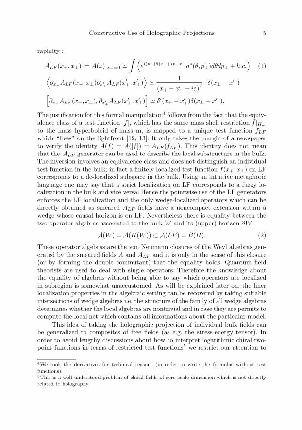
rapidity :
ALF (x+, x⊥) := A(x)|x−=0 �∫ (
ei(p−(θ)x++ip⊥x⊥a∗(θ, p⊥)dθdp⊥ + h.c.)
(1)⟨∂x+ALF (x+, x⊥)∂x′
+ALF (x′
+, x′⊥)⟩� 1(
x+ − x′+ + iε
)2 · δ(x⊥ − x′⊥)[
∂x+ALF (x+, x⊥), ∂x′+ALF (x′
+, x′⊥)]� δ′(x+ − x′
+)δ(x⊥ − x′⊥).
The justification for this formal manipulation4 follows from the fact that the equiv-alence class of a test function [f ], which has the same mass shell restriction f |Hm
to the mass hyperboloid of mass m, is mapped to a unique test function fLF
which “lives” on the lightfront [12, 13]. It only takes the margin of a newspaperto verify the identity A(f) = A([f ]) = ALF (fLF ). This identity does not meanthat the ALF generator can be used to describe the local substructure in the bulk.The inversion involves an equivalence class and does not distinguish an individualtest-function in the bulk; in fact a finitely localized test function f(x+, x⊥) on LFcorresponds to a de-localized subspace in the bulk. Using an intuitive metaphoriclanguage one may say that a strict localization on LF corresponds to a fuzzy lo-calization in the bulk and vice versa. Hence the pointwise use of the LF generatorsenforces the LF localization and the only wedge-localized operators which can bedirectly obtained as smeared ALF fields have a noncompact extension within awedge whose causal horizon is on LF. Nevertheless there is equality between thetwo operator algebras associated to the bulk W and its (upper) horizon ∂W
A(W ) = A(H(W )) ⊂ A(LF ) = B(H). (2)
These operator algebras are the von Neumann closures of the Weyl algebras gen-erated by the smeared fields A and ALF and it is only in the sense of this closure(or by forming the double commutant) that the equality holds. Quantum fieldtheorists are used to deal with single operators. Therefore the knowledge aboutthe equality of algebras without being able to say which operators are localizedin subregion is somewhat unaccustomed. As will be explained later on, the finerlocalization properties in the algebraic setting can be recovered by taking suitableintersections of wedge algebras i.e. the structure of the family of all wedge algebrasdetermines whether the local algebras are nontrivial and in case they are permits tocompute the local net which contains all informations about the particular model.
This idea of taking the holographic projection of individual bulk fields canbe generalized to composites of free fields (as e.g. the stress-energy tensor). Inorder to avoid lengthy discussions about how to interpret logarithmic chiral two-point functions in terms of restricted test functions5 we restrict our attention to
4We took the derivatives for technical reasons (in order to write the formulas without testfunctions).5This is a well-understood problem of chiral fields of zero scale dimension which is not directlyrelated to holography.

6 Bert Schroer
Wick-composites of ∂x+ALF (x+, x⊥)
[BLF (x+, x⊥) , CLF (x′+, x
′⊥)]
=m∑
l=0
δl(x⊥ − x′⊥)
n(l)∑k(l)=0
δk(l)(x+ − x′+)D(k(l))
LF (x+, x⊥), (3)
where the dimensions of the composites D(k(l))LF together with the degrees of the
derivatives of the delta functions obey the standard rule of scale dimensional con-servation. In the commutator the transverse and the longitudinal part both appearwith delta functions and their derivatives yet there is a very important structuraldifference which shows up in the correlation functions. To understand this pointwe look at the second line in (1). The longitudinal (=lightlike) delta-functionscarries the chiral vacuum polarization the transverse part consists only of prod-ucts of delta functions as if it would come from a product of correlation functionsof nonrelativistic Schrodinger creation/annihilation operators ψ∗(x⊥), ψ(x⊥). Inother words the LF-fields which feature in this extended chiral theory are chimerabetween QFT and QM ; they have one leg in QFT and n-2 legs in QM with the“chimeric vacuum” being partially a (transverse) factorizing quantum mechani-cal state of “nothingness” (the Buddhist nirvana) and partially the longitudinallyparticle-antiparticle polarized LQP vacuum state of “virtually everything” (theAbrahamic heaven).
Upon lightlike localization of LF to (in the present case) ∂W (or to a longi-tudinal interval) the vacuum on A(∂W ) becomes a radiating KMS thermal statewith nonvanishing localization-entropy [13, 14]. In case of interacting fields thereis no change with respect to the absence of transverse vacuum polarization, butunlike the free case the global algebra A(LF ) or the semi-global algebra A(∂W )is generally bigger than the algebra one obtains from the globalization using com-pactly localized subalgebras, i.e. ∪O⊂LFALF (O) ⊂ A(LF ), O ⊂ LF . We willreturn to this point at a more opportune moment.
The aforementioned “chimeric” behavior of the vacuum is related in a pro-found way to the conceptual distinctions between QM and QFT [16]. Whereastransversely the vacuum is tensor-factorizing with respect to the Born localizationand therefore leads to the standard quantum mechanical concepts of entanglementand the related information theoretical (cold) entropy, the entanglement from re-stricting the vacuum to an algebra associated with an interval in lightray directionis a thermal KMS state with a genuine thermodynamic entropy. Instead of thestandard quantum mechanical dichotomy between pure and entangled restrictedstates there are simply no pure states at all. All states on sharply localized operatoralgebras are highly mixed and the restriction of global particle states (includingthe vacuum) to the W-horizon A(∂W ) results in KMS thermal states. This is theresult of the different nature of localized algebras in QFT from localized algebrasin QM [16].

Constructive Use of Holographic Projections 7
Therefore if one wants to use the terminology “entanglement” in QFT oneshould be aware that one is dealing with a totally intrinsic very strong form ofentanglement: all physically distinguished global pure states (in particular finiteenergy states in particular the vacuum) upon restriction to a localized algebrabecome intrinsically entangled and unlike in QM there is no local operation whichdisentangles.
Whereas the cold (information theoretic) entanglement is often linked to theuncertainty relation of QM, the raison d’etre behind the “hot” entanglement isthe phenomenon of vacuum polarization resulting from localization in quantumtheories with a maximal velocity. The transverse tensor factorization restricts theReeh-Schlieder theorem (also known as the “state-operator relation”). For a lon-gitudinal strip (st) on LF of a finite transverse extension the LF algebra tensor-factorizes together with the Hilbert space H = Hst ⊗Hst⊥ and the Hst projectedform of the Reeh-Schlieder theorem for a subalgebra localized within the stripcontinues to be valid.
This concept of transverse extended chiral fields can also be axiomaticallyformulated for interacting fields independently of whether those objects resultfrom a bulk theory via holographic projection or whether one wants to study QFTon (non-hyperbolic) null-surfaces. These “lightfront fields” share some importantproperties with chiral fields. In both cases subalgebras localized on subregionslead to a geometric modular theory, whereas in the bulk this property is restrictedto wedge algebras. Furthermore in both cases the symmetry groups are infinitedimensional; in chiral theories the largest possible group is (after compactification)Diff(R), whereas the transverse extended version admits besides these pure lighlikesymmetries also x⊥-x+ mixing (x⊥-dependent) symmetry transformations whichleave the commutation structure invariant.
There is one note of caution, unlike those conformal QFTs which arise aschiral projections from 2-dimensional conformal QFT, the extended chiral mod-els of QFT on the lightfront which result from holography do not come with astress-energy tensor and hence the diffeomorphism invariance beyond the Mobiusinvariance (which one gets from modular invariance, no energy momentum tensorneeded) is not automatic. This leads to the interesting question if there are con-cepts which permit to incorporate also the diffeomorphisms beyond the Mobiustransformations into a modular setting, a problem which will not be pursuit here.
We have formulated the algebraic structure of holographic projected fieldsfor bosonic fields, but it should be obvious to the reader that a generalization toFermi fields is straightforward. Lightfront holography is consistent with the factthat except for d=1+1 there are no operators which “live” on a lightray sincethe presence of the quantum mechanical transverse delta function prevents such apossibility i.e. only after transverse averaging with test functions does one get to(unbounded) operators.
It is an interesting question whether a direct “holographic projection” of in-teracting pointlike bulk fields into lightfront fields analog to (1) can be formulated,
8 Bert Schroer
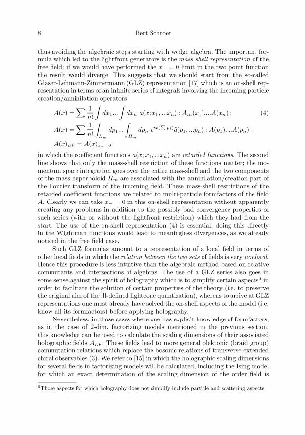
thus avoiding the algebraic steps starting with wedge algebra. The important for-mula which led to the lightfront generators is the mass shell representation of thefree field; if we would have performed the x− = 0 limit in the two point functionthe result would diverge. This suggests that we should start from the so-calledGlaser-Lehmann-Zimmermann (GLZ) representation [17] which is an on-shell rep-resentation in terms of an infinite series of integrals involving the incoming particlecreation/annihilation operators
A(x) =∑ 1
n!
∫dx1...
∫dxn a(x;x1, ...xn) : Ain(x1)....A(xn) : (4)
A(x) =∑ 1
n!
∫Hm
dp1...
∫Hm
dpn eix(∑
pi)a(p1, ...pn) : A(p1)....A(pn) :
A(x)LF = A(x)x−=0
in which the coefficient functions a(x;x1, ...xn) are retarded functions. The secondline shows that only the mass-shell restriction of these functions matter; the mo-mentum space integration goes over the entire mass-shell and the two componentsof the mass hyperboloid Hm are associated with the annihilation/creation part ofthe Fourier transform of the incoming field. These mass-shell restrictions of theretarded coefficient functions are related to multi-particle formfactors of the fieldA. Clearly we can take x− = 0 in this on-shell representation without apparentlycreating any problems in addition to the possibly bad convergence properties ofsuch series (with or without the lightfront restriction) which they had from thestart. The use of the on-shell representation (4) is essential, doing this directlyin the Wightman functions would lead to meaningless divergences, as we alreadynoticed in the free field case.
Such GLZ formulas amount to a representation of a local field in terms ofother local fields in which the relation between the two sets of fields is very nonlocal.Hence this procedure is less intuitive than the algebraic method based on relativecommutants and intersections of algebras. The use of a GLZ series also goes insome sense against the spirit of holography which is to simplify certain aspects6 inorder to facilitate the solution of certain properties of the theory (i.e. to preservethe original aim of the ill-defined lightcone quantization), whereas to arrive at GLZrepresentations one must already have solved the on-shell aspects of the model (i.e.know all its formfactors) before applying holography.
Nevertheless, in those cases where one has explicit knowledge of formfactors,as in the case of 2-dim. factorizing models mentioned in the previous section,this knowledge can be used to calculate the scaling dimensions of their associatedholographic fields ALF . These fields lead to more general plektonic (braid group)commutation relations which replace the bosonic relations of transverse extendedchiral observables (3). We refer to [15] in which the holographic scaling dimensionsfor several fields in factorizing models will be calculated, including the Ising modelfor which an exact determination of the scaling dimension of the order field is
6Those aspects for which holography does not simplify include particle and scattering aspects.
Constructive Use of Holographic Projections 9
possible. Although the holographic dimensions agree with those from the shortdistance analysis (which have been previously calculated in [18]), the conceptualstatus of holography is quite different from that of critical universality classes. Theformer is an exact relation between a 2-dimensional factorizing model (change ofthe spacetime ordering of a given bulk theory) whereas the latter is a passingto a different QFT in the same universality class. The mentioned exact result inthe case of the Ising model strengthens the hope that GLZ representations andthe closely related expansions of local fields in terms of wedge algebra generatingon-shell operators [15] have a better convergence status than perturbative series.
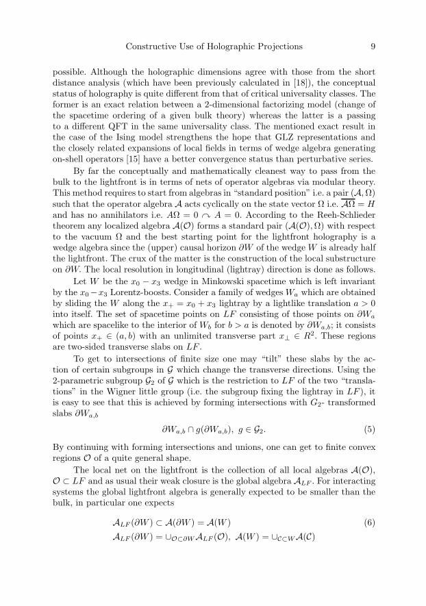
By far the conceptually and mathematically cleanest way to pass from thebulk to the lightfront is in terms of nets of operator algebras via modular theory.This method requires to start from algebras in “standard position” i.e. a pair (A,Ω)such that the operator algebra A acts cyclically on the state vector Ω i.e. AΩ = Hand has no annihilators i.e. AΩ = 0 � A = 0. According to the Reeh-Schliedertheorem any localized algebra A(O) forms a standard pair (A(O),Ω) with respectto the vacuum Ω and the best starting point for the lightfront holography is awedge algebra since the (upper) causal horizon ∂W of the wedge W is already halfthe lightfront. The crux of the matter is the construction of the local substructureon ∂W. The local resolution in longitudinal (lightray) direction is done as follows.
Let W be the x0 − x3 wedge in Minkowski spacetime which is left invariantby the x0−x3 Lorentz-boosts. Consider a family of wedges Wa which are obtainedby sliding the W along the x+ = x0 + x3 lightray by a lightlike translation a > 0into itself. The set of spacetime points on LF consisting of those points on ∂Wa
which are spacelike to the interior of Wb for b > a is denoted by ∂Wa,b; it consistsof points x+ ∈ (a, b) with an unlimited transverse part x⊥ ∈ R2. These regionsare two-sided transverse slabs on LF .
To get to intersections of finite size one may “tilt” these slabs by the ac-tion of certain subgroups in G which change the transverse directions. Using the2-parametric subgroup G2 of G which is the restriction to LF of the two “transla-tions” in the Wigner little group (i.e. the subgroup fixing the lightray in LF ), itis easy to see that this is achieved by forming intersections with G2- transformedslabs ∂Wa,b
∂Wa,b ∩ g(∂Wa,b), g ∈ G2. (5)
By continuing with forming intersections and unions, one can get to finite convexregions O of a quite general shape.
The local net on the lightfront is the collection of all local algebras A(O),O ⊂ LF and as usual their weak closure is the global algebra ALF . For interactingsystems the global lightfront algebra is generally expected to be smaller than thebulk, in particular one expects
ALF (∂W ) ⊂ A(∂W ) = A(W ) (6)
ALF (∂W ) = ∪O⊂∂WALF (O), A(W ) = ∪C⊂WA(C)
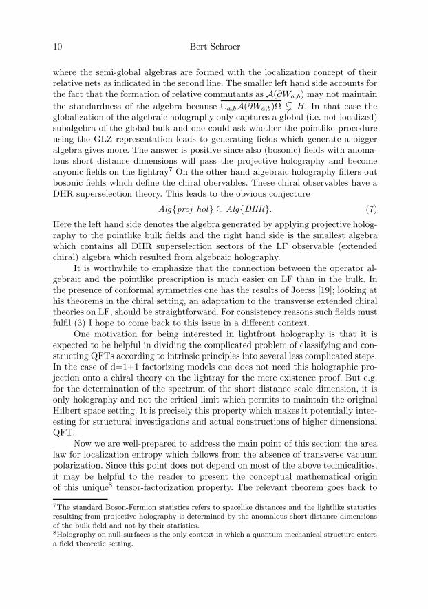
10 Bert Schroer
where the semi-global algebras are formed with the localization concept of theirrelative nets as indicated in the second line. The smaller left hand side accounts forthe fact that the formation of relative commutants as A(∂Wa,b) may not maintainthe standardness of the algebra because ∪a,bA(∂Wa,b)Ω � H. In that case theglobalization of the algebraic holography only captures a global (i.e. not localized)subalgebra of the global bulk and one could ask whether the pointlike procedureusing the GLZ representation leads to generating fields which generate a biggeralgebra gives more. The answer is positive since also (bosonic) fields with anoma-lous short distance dimensions will pass the projective holography and becomeanyonic fields on the lightray7 On the other hand algebraic holography filters outbosonic fields which define the chiral obervables. These chiral observables have aDHR superselection theory. This leads to the obvious conjecture
Alg{proj hol} ⊆ Alg{DHR}. (7)
Here the left hand side denotes the algebra generated by applying projective holog-raphy to the pointlike bulk fields and the right hand side is the smallest algebrawhich contains all DHR superselection sectors of the LF observable (extendedchiral) algebra which resulted from algebraic holography.
It is worthwhile to emphasize that the connection between the operator al-gebraic and the pointlike prescription is much easier on LF than in the bulk. Inthe presence of conformal symmetries one has the results of Joerss [19]; looking athis theorems in the chiral setting, an adaptation to the transverse extended chiraltheories on LF, should be straightforward. For consistency reasons such fields mustfulfil (3) I hope to come back to this issue in a different context.
One motivation for being interested in lightfront holography is that it isexpected to be helpful in dividing the complicated problem of classifying and con-structing QFTs according to intrinsic principles into several less complicated steps.In the case of d=1+1 factorizing models one does not need this holographic pro-jection onto a chiral theory on the lightray for the mere existence proof. But e.g.for the determination of the spectrum of the short distance scale dimension, it isonly holography and not the critical limit which permits to maintain the originalHilbert space setting. It is precisely this property which makes it potentially inter-esting for structural investigations and actual constructions of higher dimensionalQFT.
Now we are well-prepared to address the main point of this section: the arealaw for localization entropy which follows from the absence of transverse vacuumpolarization. Since this point does not depend on most of the above technicalities,it may be helpful to the reader to present the conceptual mathematical originof this unique8 tensor-factorization property. The relevant theorem goes back to
7The standard Boson-Fermion statistics refers to spacelike distances and the lightlike statisticsresulting from projective holography is determined by the anomalous short distance dimensionsof the bulk field and not by their statistics.8Holography on null-surfaces is the only context in which a quantum mechanical structure entersa field theoretic setting.
Constructive Use of Holographic Projections 11
Borchers [20] and can be stated as follows. Let Ai ⊂ B(H), i = 1, 2 be two operatoralgebras with [A1, U(a)A2U(a)∗] = 0 ∀a and U(a) a translation with nonnegativegenerator which fulfils the cluster factorization property (i.e. asymptotic factoriza-tion in correlation functions for infinitely large cluster separations) with respectto a unique U(a)-invariant state vector Ω9. It then follows that the two algebrastensor factorize in the sense A1∨A2 = A1⊗A2 where the left hand side denotesthe joint operator algebra.
In the case at hand the tensor factorization follows as soon as the open re-gions Oi ⊂ LF in A(Oi) i = 1, 2 have no transverse overlap. The lightlike clusterfactorization is weaker (only a power law) than its better known spacelike coun-terpart, but as a result of the analytic properties following from the non-negativegenerator of lightlike translations it enforces the asymptotic factorization to bevalid at all distances. The resulting transverse factorization implies the transverseadditivity of extensive quantities as energy and entropy and their behavior in ligh-tray direction can then be calculated in terms of the associated auxiliary chiraltheory. A well-known property for spacelike separations.
This result [13, 14] of the transverse factorization may be summarized asfollows:
1. The system of LF subalgebras {A(O)}O⊂LF tensor-factorizes transverselywith the vacuum being free of transverse entanglement
A(O1∪O2) = A(O1)⊗A(O2), (O1)⊥ ∩ (O2)⊥ = ∅ (8)
〈Ω |A(O1)⊗A(O2)|Ω〉 = 〈Ω |A(O1) |Ω〉 〈Ω| A(O2)|Ω〉 .2. Extensive properties as entropy and energy on LF are proportional to the
extension of the transverse area.3. The area density of localization-entropy in the vacuum state for a system
with sharp localization on LF diverges logarithmically
sloc = limε→0
c
6|ln ε|+ ... (9)
where ε is the size of the interval of “fuzziness” of the boundary in the lightraydirection which one has to allow in order for the vacuum polarization cloud toattenuate and the proportionality constant c is (at least in typical examples)the central extension parameter of the Witt-Virasoro algebra.
The following comments about these results are helpful in order to appreciatesome of the physical consequences as well as extensions to more general null-surfaces.
As the volume divergence of the energy/entropy in a heat bath thermal sys-tem results from the thermodynamic limit of a sequence of boxed systems in aGibbs states, the logarithmic divergence in the vacuum polarization attenuation
9Locality in both directions shows that the lightlike translates 〈Ω |AU(a)B|Ω〉 are boundaryvalues of entire functions and the cluster property together with Liouville’s theorem gives thefactorization.

12 Bert Schroer
distance ε plays an analogous role in the approximation of the semiinfinitely ex-tended ∂W by sequences of algebras whose localization regions approach ∂W fromthe inside. In both cases the limiting algebras are monads whereas the approxi-mands are type I analogs of the “box quantization” algebras. In fact in the presentconformal context the relation between the standard heat bath thermodynamiclimit and the limit of vanishing attenuation length for the localization-caused vac-uum polarization cloud really goes beyond an analogy and becomes an isomor-phism.
This surprising result is based on two facts [13, 14]. On the one hand con-formal theories come with a natural covariant “box” approximation of the ther-modynamic limit since the continuous spectrum translational Hamiltonian canbe obtained as a scaled limit of a sequence of discrete spectrum conformal rota-tional Hamiltonians associated to global type I systems. On the other hand it hasbeen known for some time that a heat bath chiral KMS state can always be re-interpreted as the Unruh restriction applied to a vacuum system in an larger world(a kind of inverse Unruh effect). Both facts together lead to the above formula forthe area density of entropy. In fact using the conformal invariance one can writethe area density formula in the more suggestive manner by identifying ε with theconformal invariant cross-ratio of 4 points
ε2 =(a2 − a1) (b1 − b2)(b1 − a1) (b2 − a2)
where a1 < a2 < b2 < b1 so that (a1, b1) corresponds to the larger localizationinterval and (a2, b2) is the approximand which goes with the interpolating typeI algebras. At this point one makes contact with some interesting work on whatcondensed matter physicist call the “entanglement entropy”10.
One expects that the arguments for the absence of transverse vacuum fluctu-ations carry over to other null-surfaces as e.g. the upper horizon ∂D of the doublecone D. In the interacting case it is not possible to obtain ∂D generators throughtest function restrictions. For zero mass free fields there is, however, the possibilityto conformally transform the wedge into the double cone and in this way obtainthe holographic generators as the conformally transformed generators of A(∂W ).In order to show that the resulting A(∂D) continue to play their role even whenthe bulk generators cease to be conformal one would have to prove that certaindouble-cone affiliated inclusions are modular inclusions. We hope to return to thisinteresting problem.
10In [21] the formula for the logarithmically increasing entropy is associated with a field theoreticcutoff and the role of the vacuum polarization cloud in conjunction with the KMS thermalproperties (which is not compatible with a quantum mechanical entanglement interpretation [16])are not noticed. Since there is no implementation of the split property, the idea of an attenuationof the vacuum polarization cloud has no conceptual place in a path integral formulation. QM andQFT are not distinguished in the functional integral setting and even on a metaphorical levelthere seems to be no possibility to implement the split property.

Constructive Use of Holographic Projections 13
We have presented the pointlike approach and the algebraic approach nextto each other, but apart from the free field we have not really connected them.Although one must leave a detailed discussion of their relation to the future, thereare some obvious observations one can make. Since for chiral fields the notion ofshort-distance dimension and rotational spin (the action of the L0 generator) areclosely connected and since the algebraic process of taking relative commutatorsis bosonic, the lightfront algebras are necessarily bosonic. A field, as the chiralorder variable of the Ising model with dimension 1
16 , does not appear in the al-gebraic holography, but, as mentioned above, it is the pointlike projection of themassive order variable in the factorizing Ising model in the bulk. On the otherhand an integer dimensional field as the stress-energy tensor, is common to bothformulations. This suggests that the anomalous dimensional fields which are miss-ing in the algebraic construction may be recovered via representation theory ofthe transverse extended chiral observable algebra which arises as the image of thealgebraic holography.
Since the original purpose of holography similar to that of its ill-fated light-cone quantization predecessor, is to achieve a simplified but still rigorous descrip-tion (for the lightcone quantization the main motivation was a better descriptionof certain “short distance aspects” of QFT), the question arises if one can useholography as a tool in a more ambitious program of classification and construc-tion of QFTs. In this case one must be able to make sense of inverse holographyi.e. confront the question whether, knowing the local net on the lightfront one canonly obtain at least part of the local substructure of the bulk. It is immediatelyclear that one can construct that part in the bulk, which arises from intersectingthe LF-affiliated wedge algebras. The full net is only reconstructible if the action ofthose remaining Poincare transformations outside the 7-parametric LF covariancegroup is known.
The presence of the Mobius group acting on the lightlike direction on null-surfaces in curved spacetime resulting from bifurcate Killing horizons [22] has beenestablished in [23], thus paving the way for the transfer of the thermal results toQFT in CFT. This is an illustration of symmetry enhancement, which is one ofholographies “magics”.
The above interaction-free case with its chiral Abelian current algebra struc-ture (1) admits a much larger unitarily implemented symmetry group, namely thediffeomorphism group of the circle. However the unitary implementers (beyond theMobius group) do not leave the vacuum invariant (and hence are not Wigner sym-metries). As a result of the commutation relations (3) these Diff(S1) symmetriesare expected to appear in the holographic projection of interacting theories. Theseunitary symmetries act only geometrically on the holographic objects; their actionon the bulk (on which they are also well-defined) is fuzzy i.e. not describable ingeometric terms. This looks like an interesting extension of the new setting of localcovariance [24].
The area proportionality for localization entropy is a structural property ofLQP which creates an interesting and hopefully fruitful contrast with Bekenstein’s
14 Bert Schroer
area law [25] for black hole horizons. Bekenstein’s thermal reading of the areabehavior of a certain quantity in classical Einstein-Hilbert like field theories hasbeen interpreted as being on the interface of QFT with QG. Now we see that themain support, namely the claim that QFT alone cannot explain an area behavior,is not correct. There remains the question whether Bekenstein’s numerical value,which people tried to understand in terms of quantum mechanical level occupation,is a credible candidate for quantum entropy. QFT gives a family of area laws withdifferent vacuum polarization attenuation parameters ε and it is easy to fix thisparameter in terms of the Planck length so that the two values coalesce. Theproblem which I have with such an argument is that I have never seen a situationwhere a classical value remained intact after passing to the quantum theory. Thisdoes only happen for certain quasiclassical values in case the system is integrable.
3. From holography to correspondence: the AdS/CFTcorrespondence and a controversy
The holography onto null-surfaces addresses the very subtle relation between bulkquantum matter and the projection onto its causal/event horizon as explained inthe previous section. A simpler case of holography arises if the bulk and a lowerdimensional brane11 (timelike) boundary share the same maximally possible space-time (vacuum) symmetry. The only case where this situation arises between twoglobal Lorentz manifolds of different spacetime dimension is the famous AdS/CFTcorrespondence. In that case the causality leakage off a brane does not occur. In thefollowing we will use the same terminology for the universal coverings of AdS/CFTas for the spacetimes themselves.
Already in the 60s the observation that the 15-parametric conformal sym-metry which is shared between the conformal 3 + 1-dimensional compactifiedMinkowski spacetime and the 5-dimensional Anti-de-Sitter space (the negativeconstant curvature brother of the cosmologically important de Sitter spacetime)brought a possible field theoretic relation between these theories into the fore-ground; in fact Fronsdal [26] suspected that QFTs on both spacetimes share morethan the spacetime symmetry groups. But the modular localization theory whichcould convert the shared group symmetry into a relation between two differentspacetime ordering devices (in the sense of Leibniz) for the same abstract quantummatter substrate was not yet in place at that time. Over several decades the mainuse of the AdS solution has been (similar to Godel’s cosmological model) to showthat the Einstein-Hilbert field equations, besides the many desired solution (asthe Robertson-Walker cosmological models and the closely related de Sitter space-time), also admit unphysical solutions (leading to timelike selfclosing worldlines,time machines, wormholes etc.) and therefore should be further restricted.
11In general the brane has a lower dimensional symmetry than its associated bulk and usuallydenotes a d − 1 dimensional subspace which contains a time-like direction. Different from null-surfaces branes have a causal leakage.
Constructive Use of Holographic Projections 15
The AdS spacetime lost this role of only providing counterexamples and be-gan to play an important role in particle physics when the string theorist placed itinto the center of a conjecture about a correspondence between a particular maxi-mally supersymmetric massless conformally covariant Yang-Mills model in d=1+3and a supersymmetric gravitational model. The first paper was by J. Maldacena[27] who started from a particular compactification of 10-dimensional superstringtheory, with 5 uncompactified coordinates forming the AdS spacetime. Since themathematics as well as the conceptual structure of string theory is poorly under-stood, the string side was identified with one of the supersymmetric gravity modelswhich in spite of its being non-renormalizable admitted a more manageable La-grangian formulation and was expected to have a similar particle content. On theside of CFT he placed a maximally supersymmetric gauge theory of which calcu-lations which verify the vanishing of the low order beta function already existed12
(certainly a necessary prerequisite for conformal invariance). The arguments in-volved perturbation theory and additional less controllable approximations. Themore than 4.700 follow up papers on this subject did essentially not change thestatus of the conjecture. But at least some aspects of the general AdS/CFT cor-respondence became clearer after Witten [28] exemplified the ideas in the fieldtheoretic context of a Φ4 coupling on AdS using a Euclidean functional integralsetting.
The structural properties of the AdS/CFT correspondence came out clearlyin Rehren’s [30] algebraic holography. The setting of local quantum physics (LQP)is particularly suited for questions in which one theory is assumed as given andone wants to construct its holographic projection or its corresponding model onanother spacetime. LQP can solve such problems of isomorphisms between modelswithout being forced to actually construct a model on either side (which functionalintegration proposes to do but only in a metaphoric way). At first sight Rehren’ssetting rewritten in terms of functional integrals (with all the metaphoric caveats,but done in the best tradition of the functional trade) looked quite different fromWitten’s functional representation. But thanks to a functional identity (explainedin the Dutsch-Rehren paper), which shows that fixing functional sources on aboundary and forcing the field values to take on a boundary value via delta functionin the functional field space leads to the same result. In this way the apparentdisparity disappeared [31] and there is only one AdS/CFT correspondence withinQFT.
There are limits to the rigor and validity of functional integral tools in QFT.Even in QM where they are rigorous an attempt to teach a course on QM basedon functional integrals would end without having been able to cover the standardmaterial. As an interesting mental exercise just image a scenario with Feynmanbefore Heisenberg. Since path integral representations are much closer to the old
12An historically interesting case in which the beta function vanishes in every order is the massiveThirring model. In that case the zero mass limit is indeed conformally invariant, but there isno interacting conformal theory for which a perturbation can be formulated directly, it wouldgenerate unmanageable infrared divergencies.

16 Bert Schroer
quasiclassical Bohr Sommerfeld formulation the transition would have been muchsmoother, but it would have taken a longer time to get to the operational coreof quantum theory; on the other hand quasiclassical formulas and perturbativecorrections thereof would emerge with elegance and efficiency.
Using the measure theoretical functional setting it is well-known that su-perrenormalizable polynomial couplings can be controlled this way [35]. Realis-tic models with infinite wave function renormalization constants (all realistic La-grangian models in more than two spacetime dimensions have a trans-canonicalshort distance behavior) do not fall into this amenable category. But even in lowdimensions, where there exist models with finite wave function renormalizationconstants and hence the short distance prerequisites are met, the functional set-ting of the AdS/CFT correspondence has an infrared problem1314 of a nasty unre-solved kind [37]. As the result of lack of an analog to the operator formulation inQM the suggestive power, their close relation to classical geometric concepts andtheir formal elegance functional integrals have maintained their dominant role inparticle physics although renormalized perturbation theory is better taken care ofin the setting of “causal perturbation”.15 An operator approach which is not onlycapable to establish the mathematical existence of models but also permits theirexplicit construction exists presently only in d = 1 + 1; it is the previously men-tioned bootstrap-formfactor or wedge-localization approach for factorizing models.Lagrangian factorizing models only constitute a small fraction.
For structural problems as holography, where one starts from a given the-ory and wants to construct its intrinsically defined holographic image, the useof metaphorical instruments as Euclidean functional integral representations issuggestive but not really convincing in any mathematical sense. As in the case oflightfront holography there are two mathematically controllable ways to AdS/CFTholography; either using (Wightman) fields (projective holography) or using oper-ator algebras (algebraic holography). The result of all these different methods canbe consistently related [31, 32].
The main gain in lightfront holography is a significant simplification of certainproperties as compared to the bulk. Even if some of the original problems of thebulk come back in the process of holographic inversion they reappear in the moreamenable form of several smaller problems rather than one big one.
The motivation for field theorists being interested in the AdS/CFT correspon-dence is similar, apart from the fact that the simplification obtainable through analgebraic isomorphism is more limited (less radical) than that of a projection.
13Infrared problems of the kind as they appear in interacting conformal theories are strictlyspeaking not susceptible to perturbation theoretical treatment and they also seem to pose serious(maybe insoluble) problems in functional integral representations. In those cases where on knowsthe exact form of the massless limit (Thirring model) this knowledge can be used to disentanglethe perturbative infrared divergences.14Eds. annotation: see the chapter by Gottschalk-Thaler in this volume.15Eds. annotation: see the chapter by Dutsch-Brennecke in this volume.
Constructive Use of Holographic Projections 17
Nevertheless it is not unreasonable to explore the possibility whether some hid-den property as for example a widespread conjecture partial integrability16 couldbecome more visible after a spacetime “re-packaging” of the quantum matter sub-strate from CFT to AdS.
Despite many interesting analogies between chiral theories and higher di-mensional QFT [36] little is known about higher-dimensional conformal QFTs.There are Lagrangian candidates as for example certain supersymmetric Yang-Mills theories which fulfil (at least in lowest order) some perturbative prerequisiteof conformality which consists in a vanishing beta-function. As mentioned beforeperturbation theory for conformal QFT, as a result of severe infrared problems,cannot be formulated directly. The prime example for such a situation is the mas-sive Thirring model for which there exists an elegant structural argument forβ(g) = 0 and the knowledge about the non-perturbative massless version can thenbe used to find the correct perturbative infrared treatment.
As far as I could see (with apologies in case of having overlooked some im-portant work) none of these two steps has been carried out for SUSY-YM, so eventhe conformal side of the Maldacena conjecture has remained unsafe territory.
There is one advantage which null-surface holography has over AdS/CFTtype brane holography. The cardinality of degrees of freedom adjusts itself towhat is natural for null-surfaces (as a manifold in its own right); for the lightfrontholography this is the operator algebra generated from extended chiral fields (3).On the other hand this “thinning out” in holographic projections is of course thereason why inverse holography becomes more complicated and cannot be donewith the QFT on one null surface only.
In the holography of the AdS/CFT correspondence the bulk degrees of free-dom pass to a conformal brane; in contradistinction to the holography on null-surfaces there is no reduction of degrees of freedom resulting from projection.Hence the AdS/CFT isomorphism starting from a “normal” (causally completeas formally arising from Lagrangians) 5-dimensional AdS leads to a conformalfield theory with too many degrees of freedom. Since a “thinning out” by handdoes not seem to be possible, the “physically health” of such a conformal QFT issomewhat dodgy, to put it mildly.
In case one starts with a free Klein-Gordon field on AdS one finds that thegenerating conformal fields of the CFT are special generalized free fields i.e. a kindof continuous superpositions of free fields. They were introduced in the late 50s byW. Greenberg and their useful purpose was (similar to AdS in classical gravity)to test the physical soundness of axioms of QFT in the sense that if a system ofaxioms allowed such solutions, it needed to be further restricted [33] (in that casethe so-called causal completion or time-slice property excluded generalized freefields). It seems that meanwhile the word “physical” has changes its meaning, itis used for anything which originated from a physicist.
16Global integrability is only possible in d = 1 + 1, but I am not aware of any theorem whichrules out the possibility of integrable substructures.
18 Bert Schroer
In the opposite direction the degrees of freedom of a “normal” CFT become“diluted” on AdS in the inverse correspondence. There are not sufficient degrees offreedom for arriving at nontrivial compactly localized operators, the cardinality ofdegrees of freedom is only sufficient to furnish noncompact regions as AdS wedgeswith nontrivial operators, the compactly localized double cone algebras remaintrivial (multiples of the identity). In the setting based on fields this means thatthe restriction on testfunction spaces is so severe that pointlike fields AAdS(x) atinterior points x ∈ int(AdS) do not exist in the standard sense as operator-valueddistributions on Schwartz spaces. They exist on much smaller test function spaces,which contain no functions with compact localizations.
Both sides of the correspondence have been treated in a mathematically rigor-ous fashion for free AdS (Klein-Gordon equation) theories and free (wave equation)CFT [34, 32] where the mismatch between degrees of freedom can be explicatedand the structural arguments based on the principles of general QFT show thatthis mismatch between the transferred and the natural cardinality of the degreeof freedom is really there. In terms of the better known Lagrangian formalismthe statement would be that if one starts from a Lagrange theory at one side theother side cannot be Lagrangian. Of course both sides remain QFT in the moregeneral sense of fulfilling the required symmetries, have positive energy and beingconsistent with spacelike commutativity. In the mentioned free field illustration anAdS Klein-Gordon field is evidently Lagrangian whereas the corresponding confor-mal generalized free field has no Lagrangian and cannot even be characterized interms of a local hyperbolic field equation. According to the best educated guess,4-dimensional maximally supersymmetric Yang-Mills theories (if they exist andare conformal) would be natural conformal QFTs “as we know it” and thereforecannot come from a natural QFT on AdS. Needless to say again that there aresevere technical problems to set up a perturbation theory for conformally invariantinteractions, the known perturbative systematics breaks down in the presence ofinfrared problems17.
I belong to a generation for which not everything which is mathematicallypossible must have a physical realization; in particular I do not adhere to thenew credo that every mathematically consistent idea is realized in some parallelworld (anthropic principle): no parallel universe for the physical realization of everymathematical belch.
Generalized free fields18 and their interacting counterparts, which arise fromnatural AdS free- or interacting- fields, remain in my view unphysical, but are
17A well-known problem is the massive Thirring model which leads to β = 0 in all orders. In thiscase one already knew the conformal limit in closed form and was able to check the correctnessof the relation by consistency considerations.18It is interesting to note that the Nambu-Goto Lagrangian (which describes a classical relativis-tic string) yields upon quantization a pointlike localized generalized free field with the well-knowninfinite tower mass spectrum and the appearance of a Hagedorn limit temperature. As such it ispointlike localized and there is no intrinsic quantum concept which permits to associate it withany stringlike localization.

Constructive Use of Holographic Projections 19
of considerable mathematical interest. They do not fit into the standard causallocalization setting and they do not allow thermal KMS states without a limitingHagedorn temperature (both facts are related). Nature did not indicate that itlikes to go beyond the usual localizability and thermal behavior. If string theorydemands such things it is not my concern, let Max Tegmark find another universewhere nature complies with string theory.
Holography is a technical tool and not a physical principle. It simplifies cer-tain aspects of a QFT at the expense of others (i.e. it cannot achieve miracles).The use of such ideas in intermediate steps may have some technical merits, butI do not see any scientific reason to change my viewpoint about physical admis-sibility. The question of whether by changing the spacetime encoding one couldsimplify certain properties (for example detect integrable substructures) of compli-cated theories is of course very interesting, but in order to pursue such a line it isnot necessary to physically identify the changed theory. Such attempts, where onlyone side needs to be physical and the role of holography would consist in expos-ing certain structural features which remained hidden in the original formulation,sound highly interesting to me.
There is however one deeply worrisome aspect of this whole development.Never before has there been more than 4.700 publication on such a rather narrowsubject; in fact even nowadays, one decade after this gold-digger’s rush aboutthe AdS/CFT correspondence started, there is still a sizable number of papersevery month by people looking for nuggets at the same place but without bringingMaldacena’s gravity-gauge theory conjecture any closer to a resolution. Even withmaking all the allowances in comparison with earlier fashions, this phenomenonis too overwhelming in order to be overlooked. Independent of its significance forparticle physics and the way it will end, the understanding of what went on and itscovering by the media will be challenging to historians and philosophers of sciencein the years to come.
I know that it is contra bonos mores to touch on a sociological aspect in aphysics paper, but my age permits me to say that at no time before was the scien-tific production in particle theory that strongly coupled to the Zeitgeist as duringthe last two decades; never before had global market forces such a decisive impacton the scientific production. Therefore it is natural to look for an explanation whythousands of articles are written on an interesting (but not clearly formulated)conjecture with hundreds of other interesting problems left aside; where does themagic attraction come from? Is it the Holy Grail of a TOE which sets into mo-tion these big caravans? Did the critical power of past particle physics disappearin favor of acclamation? Why are the few critical but unbiased attempts onlymentioned by the labels given to them and not by their scientific content?
Since commentaries about the crisis in an area of which one is part run therisk of being misunderstood, let me make perfectly clear that particle physics was aspeculative subject and I uphold that it must remain this way. Therefore I have noproblem whatsoever with Maldacena’s paper; it is in the best tradition of particlephysics, which was always a delicate blend of a highly imaginative and innovative

20 Bert Schroer
contribution from one author with profoundly critical analysis of others. I amworried about the loss of this balance. My criticism is also not directed againstthe thousands of authors who enter this area in good faith believing that they areworking at an epoch-forming paradigmatic problem because their peers gave themthis impression. Even if they entered for the more mundane reason of carving outa career, I would not consider this as the cause of the present problem.
The real problem is with those who by their scientific qualifications andstatus are the intellectual leaders and the role models. If they abdicate their roleas critical mediators by becoming the whips of the TOE monoculture of particlephysics, then checks and balances will be lost. Would there have been almost 5000publication, on a rather narrow theme (compared with other topics) in the presenceof a more critical attitude from leading particle physicists? No way. Would particletheory, once the pride of theoretical physics with a methodological impact on manyadjacent areas, have fallen into disrespect and be the object of mock within thelarger physics community? The list of questions of this kind with negative answerscan be continued.
It is worthwhile to look back at times when the delicate balance between theinnovative and speculative on the one hand and the critical on the other was stillthere. Young researchers found guidance by associating themselves to “schools ofthought” which where associated with geographical places and names as Schwinger,Landau, Bogoliubov, Wheeler, Wightman, Lehmann, Haag... who represented dif-ferent coexisting schools of thought. Instead of scientific cross fertilization betweendifferent schools, the new globalized caravan supports the formation of a giganticmonoculture and the loss of the culture of checks and balances.
Not even string theorists can deny that this unfortunate development startedwith string theory. Every problem string theory addresses takes on a strangemetaphoric aspect, an effect which is obviously wanted as the fondness for theuse of the letter M shows. The above mentioned AdS/CFT topic gives an illus-tration, which, with a modest amount of mathematical physics shows, the clearstructural QFT theorem as compared to the strange conjecture which even thou-sands of publications were not able to liberate from the metaphoric twilight.
But it is a remarkable fact that, whenever string theorist explain their ideasby QFT analogs in the setting of functional integrals, as was done by Witten in[28] for the ϕ4 coupling, and on the other hand algebraic quantum field theoristspresent their rigorous structural method for the same model in the same setting[31], the two results agree (see also [37]).
This is good news. But now comes the bad news. Despite the agreement theWitten camp, i.e. everybody except a few individuals, claim that there exist twodifferent types of AdS/CFT correspondences namely theirs and another one whichat least some of them refer to as the “German AdS/CFT correspondence”. Whyis that? I think I know but I will not write it.
At this point it becomes clear that it is the abandonment of the critical roleof the leaders which is fuelling this unhealthy development. Could a statement:“X-Y-Z theory is a gift of the 21st century which by chance fell into the 20 century”
Constructive Use of Holographic Projections 21
have come from Pauli, Schwinger, or Feynman? One would imagine that in thosedays people had a better awareness that mystifications like this could disturb thedelicate critical counterbalance which the speculative nature of particle physicsrequires. The long range negative effect on particle theory of such a statement isproportional to the prominence and charisma of its author.
There have been several books which criticize string theory. Most critics em-phasize that the theory has not predicted a single observable effect and that thereis no reason to expect that this will change in the future. Although I sympathizewith that criticism, especially if it comes from experimentalists and philosophers,I think that a theorist should focus his critique on the conceptual and mathemat-ical structure and not rely on help from Karl Popper or dwell on the non-existentobservational support. Surprisingly I could not find any scholarly article in thisdirection. One of the reasons may be that after 4 decades of development of stringtheory such a task requires rather detailed knowledge about its conceptual andmathematical basis. As a result of this unsatisfactory situation I stopped my crit-ical article [29] from going into print and decided to re-write it in such a way thatthe particle physics part is strengthened at the expense of the sociological sections.
The aforementioned situation of ignoring results which shed a critical lighton string theory or the string theorists version of the AdS/CFT correspondence isperhaps best understood in terms of the proverbial executing of the messenger whobrings bad news ; the unwanted message in the case at hand being the structuralimpossibility to have Lagrangian QFTs with causal propagation on both sides ofthe correspondence.
It seems that under the corrosive influence of more than 4 decades of stringtheory, Feynman’s observation about its mode of arguing being based on findingexcuses instead of explanations, which two decades ago was meant to be provoca-tive, has become the norm. The quantum gravity-gauge theory conjecture is agood example of how a correct but undesired AdS/CFT correspondence is shiftedto the elusive level of string theory and quantum gravity so that the degrees offreedom aspect becomes pushed underneath the rug of the elusive string theory,where it only insignificantly enlarges the already very high number of metaphors.
There have been an increasing number of papers with titles as “QCD anda Holographic Model of Hadrons”, “Early Time Dynamics in Heavy Ion Colli-sions and AdS/CFT Correspondence”, “Confinement/Deconfinement Transitionin AdS/CFT”, “Isospin Diffusion in Thermal AdS/CFT with Flavour”, “Holo-graphic Mesons in a Thermal Bath”, “Viscous Hydrodynamics and AdS/CFT”,“Heavy Quark Diffusion from AdS/CFT” . . . Ads/CFT for everything? Is stringtheory bolstered by AdS/CFT really on the way to become a TOE for all ofphysics, a theory for anything which sacrifices conceptual cohesion to amok run-ning calculations? Or are we witnessing a desperate attempt to overcome the morethan 4 decade lasting physical disutility? Perhaps it is only a consequence of the“liberating” effect of following prominent leaders who have forgone their duty ascritical mediators and preserver of conceptual cohesion.
22 Bert Schroer
4. Concluding remarks
In these notes we revisited one of the oldest and still unsolved conceptual problemsin QFT, the existence of interacting models. Besides some new concrete resultsabout the existence of factorizing models (which only exist in d = 1 + 1), it is thenew method itself, with its promise to explore new fundamental and fully intrinsicproperties of QFT, which merits attention. A particularly promising approach forthe classification and construction of QFTs consists in using holographic lightfrontprojections (and in a later stage work one’s way back into the bulk). In thissituation the holographic degrees of freedom are thinned out as compared to thebulk i.e. the extended chiral fields have lesser number of degrees of freedom.
The concept of degrees of freedom used here is a dynamical one. Knowingonly a global algebra19 as the wedge algebra i.e. A(W ) ⊂ B(H) as an inclusion intothe full algebra one uses fewer degrees freedom than one needs in order to describethe full local substructure of A(W ) i.e. knowing A(W ) in the sense of a local net.The degrees of freedom emerge always from relations between algebras whereasthe single algebra is a structureless monad [15]. Saying that the net A(LF ) hasless degrees of freedom than the net associated with the bulk is the same as sayingthat the knowledge of the LF affiliated wedges does not suffice to reconstructthe local bulk structure. In this sense the notion of degrees of freedom dependson the knowledge one has about a system; refining the net structure of localizedsubalgebras of a global algebra increases the degrees of freedom.
The lightfront holography is a genuine projection with a lesser cardinality ofdegrees of freedom i.e. without knowing how other Poincare transformations out-side the 7-parametric invariance group of the lightfront act it is not uniquely invert-ible. On its own, i.e. without added information, the lightfront holography cannotdistinguish between massive and massless theories; a transverse extended chiraltheory does not know whether the bulk was massive or massless. The knowledgeof how the opposite lightray translation U(a−) acts on A(LF ) restores unique-ness; but this action is necessarily “fuzzy” i.e. non-geometric, purely algebraic.Only upon returning to the spacetime ordering device in terms of the bulk itbecomes geometric.
The hallmark of null-surface holography is an area law for localization en-tropy in which the proportionality constant is a product of a holographic matterdependent constant times a logarithmic dependence on the attenuation length forvacuum polarization.
By far the more popular holography has been the AdS/CFT correspondence.Here its physical utility is less clear than the mathematical structure.
Is there really a relation between a special class of conformal gauge invariantgauge theories with supersymmetric quantum gravity? Not a very probable con-sequence of a change of an spacetime ordering device for a given matter substratewhich is what holography means. Integrable substructures within such conformal
19Knowing an operator algebra means knowing its position within the algebra B(H) of all oper-ators. Knowing its net substructure means knowing the relative position of all its subalgebras.
Constructive Use of Holographic Projections 23
gauge theories which become more overt on the AdS-side? This appears a bit morerealistic, but present indications are still very flimsy.
Acknowledgements
I am indebted to B. Fauser, J. Tolksdorf and E. Zeidler for the invitation toparticipate in a 2007 conference in Leipzig and for hospitality extended to meduring my stay.
References
[1] R. Haag and J. A. Swieca, Commun. Math. Phys. 1, (1965) 308
[2] D. Buchholz and E. H. Wichmann, Commun. Math. Phys. 106, (1986) 321
[3] B. Schroer, Particle physics in the 60s and 70s and the legacy of contributions by J.A. Swieca, arXiv:0712.0371
[4] B. Schroer, Ann. Phys. 295, (1999) 190
[5] G. Lechner, An Existence Proof for Interacting Quantum Field Theories with a Fac-torizing S-Matrix, math-ph/0601022
[6] H.-J. Borchers, D. Buchholz and B. Schroer, Commun. Math. Phys. 219, (2001) 125,hep-th/0003243
[7] S. Aks; Journ. Math. Phys. 6 (1965) 516
[8] D. Buchholz and S. J. Summers, String– and Brane–Localized Causal Fields in aStrongly Nonlocal Model, arXiv:math-ph/0512060
[9] H. Grosse and G. Lechner, JETP 11, (2007) 021
[10] Works by Buchholz and Summers as well as by Grosse and Lechner, in preparation.
[11] H. Leutwyler, Acta Phys. Austr., Suppl.V. H. Leutwyler in: Magic without Magic(J. R. Klauder ed.). Freeman, 1972. F. Jegerlehner, Helv. Phys. Acta 46, (1974) 824
[12] W. Driessler, Acta Phys. Austr. 46, (1977) 63
[13] B. Schroer, Class. Quant. Grav. 23 (2006) 5227, hep-th/0507038 and previous workcited therein
[14] B. Schroer, Class. Quant. Grav. 24 (2007), 1
[15] B. Schroer, Holography on null-surfaces, entanglement and localization entropy,arXiv:0712.4403
[16] B. Schroer, Localization and the interface between quantum mechanics, quantum fieldtheory and quantum gravity, arXiv:0711.4600
[17] V. Glaser, H. Lehmann and W. Zimmermann, Nuovo Cimento 6, (1957) 1122
[18] H. Babujian and M. Karowski, Int. J. Mod. Phys. A1952, (2004) 34
[19] M. Joerss, Lett. Math. Phys. 38, (1996) 257
[20] H-J Borchers, Commun. Math. Phys. 2, (1966) 49
[21] J.L. Cardy, O.A. Castro-Alvaredo and B. Doyon, Form factors of branch-point twistfields in quantum integrable models and entanglement entropy, hep-th/0706.3384 andthe previous literature cited therein

24 Bert Schroer
[22] B. Kay and R. Wald, Phys. Rep. 207 (1991) 49
[23] D. Guido, R. Longo and H-W Wiesbrock, Commun. math. Phys. 192, (1998) 217
[24] R. Brunetti, K. Fredenhagen and R. Verch, Commun. math. Phys. 237, (2003) 31
[25] J.D. Bekenstein, Phys. Rev. D 7, (1973) 2333
[26] C. Fronsdal, Phys. Rev. D10, (1974) 84
[27] J. Maldacena, Adv. Theor. Math. Phys. 2 (1998) 231
[28] E. Witten, Adv. Theor. Math. Phys. 2, 253-291 (1998) 20
[29] B. Schroer, String theory and the crisis in particle physics, arXiv:physics/0603112
[30] K-H Rehren, Annales Henri Poincare 1 (2000) 607, hep-th/9905179,
[31] M. Dutsch and K-H Rehren, Lett. Math. Phys. 62, 171-184 (2002)
[32] K-H Rehren, QFT Lectures on AdS-CFT, hep-th/0411086
[33] R. Haag and B. Schroer, J. Math. Phy. 3, (1962) 248
[34] M. Dutsch and K-H Rehren, Ann. Henri Poincare 4, (2003) 613
[35] J. Glimm and A. Jaffe, Jour. Math. Phys. 13, (1972) 1568
[36] N. M. Nikolov, K.-H. Rehren, I. Todorov, Harmonic bilocal fields generated by globallyconformal invariant scalar fields, arXiv:0704.1960
[37] H. Gottschalk and H. Thaler, AdS/CFT correspondence in the Euclidean context,arXiv:math-ph/0611006
Bert SchroerCBPFRua Dr. Xavier Sigaud 15022290-180 Rio de JaneiroBrazilandInstitut fur Theoretische Physikder FU BerlinGermany
Quantum Field TheoryB. Fauser, J. Tolksdorf and E. Zeidler, Eds., 25–47c© 2009 Birkhauser Verlag Basel/Switzerland
Topos Theory and ‘Neo-Realist’Quantum Theory
Andreas Doring
Abstract. Topos theory, a branch of category theory, has been proposed asmathematical basis for the formulation of physical theories. In this article, wegive a brief introduction to this approach, emphasizing the logical aspects.Each topos serves as a ‘mathematical universe’ with an internal logic, whichis used to assign truth-values to all propositions about a physical system. Weshow in detail how this works for (algebraic) quantum theory.
Mathematics Subject Classification (2000). Primary 03G30; Secondary 81P10;81T05; 83C45.
Keywords. topoi, internal logic, subobjects, truth values, daseinisation, con-texts, ‘neo-realist’ quantum theory, foundation of quantum theory, quantumgravity.
“The problem is all inside your head”, she said to methe answer is easy if you take it logically
Paul Simon (from ‘50 Ways To Leave Your Lover’)
1. Introduction
The use of topos theory in the foundations of physics and, in particular, the foun-dations of quantum theory was suggested by Chris Isham more than 10 yearsago in [14]. Subsequently, these ideas were developed in an application to theKochen-Specker theorem (with Jeremy Butterfield, [15, 16, 18, 19], for conceptualconsiderations see [17]). In these papers, the use of a multi-valued, contextual logicfor quantum theory was proposed. This logic is given by the internal logic of a cer-tain topos of presheaves over a category of contexts. Here, contexts typically are

26 Andreas Doring
abelian parts of a larger, non-abelian structure. There are several possible choicesfor the context category. We will concentrate on algebraic quantum theory and usethe category V(R) of abelian von Neumann subalgebras of the non-abelian vonNeumann algebra of observables R of the quantum system, as first suggested in[18].
The use of presheaves over such a category of contexts is motivated bythe very natural construction of the spectral presheaf Σ, which collects all theGel’fand spectra of the abelian subalgebras V ∈ V(R) into one larger structure.The Gel’fand spectra can be seen as ‘local state spaces’, and the spectral presheafserves as a state space analogue for quantum theory. Interestingly, as Isham andButterfield showed, this presheaf is not like a space: it has no points (in a category-theoretical sense), and this fact is exactly equivalent to the Kochen-Specker theo-rem.
The topos approach was developed considerably in the series of papers [5,6, 7, 8] by Chris Isham and the author. In these papers, it was shown how topostheory can serve as a new mathematical framework for the formulation of physicaltheories. The basic idea of the topos programme is that by representing the relevantphysical structures (states, physical quantities and propositions about physicalquantities) in suitable topoi, one can achieve a remarkable structural similaritybetween classical and quantum physics. Moreover, the topos programme is generalenough to allow for major generalizations. Theories beyond classical and quantumtheory are conceivable. Arguably, this generality will be needed in a future theoryof quantum gravity, which is expected to go well beyond our conventional theories.
In this paper, we will concentrate on algebraic quantum theory. We brieflymotivate the mathematical constructions and give the main definitions.1 Through-out, we concentrate on the logical aspects of the theory. We will show in detailhow, given a state, truth-values are assigned to all propositions about a quantumsystem. This is independent of any measurement or observer. For that reason, wesay that the topos approach gives a ‘neo-realist’ formulation of quantum theory.
1.1. What is a topos?
It is impossible to give even the briefest introduction to topos theory here. At thedanger of being highly imprecise, we restrict ourselves to mentioning some aspectsof this well-developed mathematical theory and give a number of pointers to theliterature. The aim merely is to give a very rough idea of the structure and internallogic of a topos. In the next subsection, we argue that this mathematical structuremay be useful in physics.
There are a number of excellent textbooks on topos theory, and the readershould consult at least one of them. We found the following books useful: [25, 9,27, 20, 21, 1, 24].
1We suppose that the reader is familiar with the definitions of a category, functor and naturaltransformation.

Topos Theory and ‘Neo-Realist’ Quantum Theory 27
Topoi as mathematical universes. Every (elementary) topos E can be seen as amathematical universe. As a category, a topos E possesses a number of structuresthat generalize constructions that are possible in the category Set of sets andfunctions.2 Namely, in Set, we can construct new sets from given ones in severalways: let S, T be two sets, then we can form the cartesian product S×T , the disjointunion S � T and the exponential ST , the set of all functions from T to S. Theseconstructions turn out to be fundamental and can all be phrased in an abstract,categorical manner, where they are called finite limits, colimits and exponentials,respectively. By definition, a topos E has all of these. One consequence of theexistence of finite limits is that each topos has a terminal object, denoted by 1.This is characterized by the property that for any object A in the topos E , thereexists exactly one arrow from A to 1. In Set, a one-element set 1 = {∗} is terminal.3
Of course, Set is a topos, too, and it is precisely the topos which usuallyplays the role of our mathematical universe, since we construct our mathematicalobjects starting from sets and functions between them. As a slogan, we have: atopos E is a category similar to Set. A very nice and gentle introduction to theseaspects of topos theory is the book [25]. Other good sources are [9, 26].
In order to ‘do mathematics’, one must also have a logic, including a deductivesystem. Each topos comes equipped with an internal logic, which is of intuitionistictype. We very briefly sketch the main characteristics of intuitionistic logic and themathematical structures in a topos that realize this logic.
Intuitionistic logic. Intuitionistic logic is similar to Boolean logic, the maindifference being that the law of excluded middle need not hold. In intuitionisticlogic, there is no axiom
� a ∨ ¬a (∗)like in Boolean logic. Here, ¬a is the negation of the formula (or proposition)a. The algebraic structures representing intuitionistic logic are Heyting algebras.A Heyting algebra is a pseudocomplemented, distributive lattice4 with zero ele-ment 0 and unit element 1, representing ‘totally false’ resp. ‘totally true’. Thepseudocomplement is denoted by ¬, and one has, for all elements α of a Heytingalgebra H ,
α ∨ ¬α ≤ 1,in contrast to α ∨ ¬α = 1 in a Boolean algebra. This means that the disjunc-tion (“Or”) of a proposition α and its negation need not be (totally) true in a
2More precisely, small sets and functions between them. Small means that we do not have properclasses. One must take care in these foundational issues to avoid problems like Russell’s paradox.3Like many categorical constructions, the terminal object is fixed only up to isomorphism: anytwo one-element sets are isomorphic, and any of them can serve as a terminal object. Nonetheless,one speaks of the terminal object.4Lattice is meant in the algebraic sense: a partially ordered set L such that any two elementsa, b ∈ L have a minimum (greatest lower bound) a ∧ b and a maximum (least upper bound)a ∨ b in L. A lattice L is distributive if and only if a ∨ (b ∧ c) = (a ∨ b) ∧ (a ∨ c) as well asa ∧ (b ∨ c) = (a ∧ b) ∨ (a ∧ c) hold for all a, b, c ∈ L.
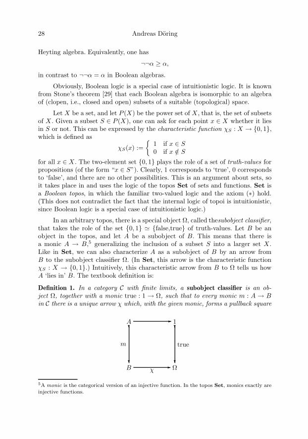
28 Andreas Doring
Heyting algebra. Equivalently, one has
¬¬α ≥ α,
in contrast to ¬¬α = α in Boolean algebras.
Obviously, Boolean logic is a special case of intuitionistic logic. It is knownfrom Stone’s theorem [29] that each Boolean algebra is isomorphic to an algebraof (clopen, i.e., closed and open) subsets of a suitable (topological) space.
Let X be a set, and let P (X) be the power set of X , that is, the set of subsetsof X . Given a subset S ∈ P (X), one can ask for each point x ∈ X whether it liesin S or not. This can be expressed by the characteristic function χS : X → {0, 1},which is defined as
χS(x) :={
1 if x ∈ S0 if x /∈ S
for all x ∈ X . The two-element set {0, 1} plays the role of a set of truth-values forpropositions (of the form “x ∈ S”). Clearly, 1 corresponds to ‘true’, 0 correspondsto ‘false’, and there are no other possibilities. This is an argument about sets, soit takes place in and uses the logic of the topos Set of sets and functions. Set isa Boolean topos, in which the familiar two-valued logic and the axiom (∗) hold.(This does not contradict the fact that the internal logic of topoi is intuitionistic,since Boolean logic is a special case of intuitionistic logic.)
In an arbitrary topos, there is a special object Ω, called thesubobject classifier,that takes the role of the set {0, 1} � {false,true} of truth-values. Let B be anobject in the topos, and let A be a subobject of B. This means that there isa monic A → B,5 generalizing the inclusion of a subset S into a larger set X .Like in Set, we can also characterize A as a subobject of B by an arrow fromB to the subobject classifier Ω. (In Set, this arrow is the characteristic functionχS : X → {0, 1}.) Intuitively, this characteristic arrow from B to Ω tells us howA ‘lies in’ B. The textbook definition is:
Definition 1. In a category C with finite limits, a subobject classifier is an ob-ject Ω, together with a monic true : 1 → Ω, such that to every monic m : A → Bin C there is a unique arrow χ which, with the given monic, forms a pullback square
B Ω�χ
A 1�
�
�
m
�
�
true
5A monic is the categorical version of an injective function. In the topos Set, monics exactly areinjective functions.

Topos Theory and ‘Neo-Realist’ Quantum Theory 29
In Set, the arrow true : 1 → {0, 1} is given by true(∗) = 1. In general, thesubobject classifier Ω need not be a set, since it is an object in the topos E , and theobjects of E need not be sets. Nonetheless, there is an abstract notion of elements(or points) in category theory that we can use. The elements of Ω are the truth-values available in the internal logic of our topos E , just like ‘false’ and ‘true’, theelements of {false,true}, are the truth-values available in the topos Set.
To understand the abstract notion of elements, let us consider sets for amoment. Let 1 = {∗} be a one-element set, the terminal object in Set. Let S bea set and consider an arrow e from 1 to S. Clearly, e(∗) ∈ S is one element of S.The set of all functions from 1 to S corresponds exactly to the elements of S. Thisidea can be generalized to other categories: if there is a terminal object 1, thenwe consider arrows from 1 to an object A in the category as elements of A. Forexample, in the definition of theindextrue!as element in a truth object subobjectclassifier the arrow true : 1 → Ω is an element of Ω. It may happen that an objectA has no elements, i.e., there are no arrows 1 → A. It is common to considerarrows from subobjects U of A to A as generalized elements, but we will not needthis except briefly in subsection 5.1.
As mentioned, the elements of the subobject classifier, understood as thearrows 1 → Ω, are the truth-values. Moreover, the set of these arrows forms aHeyting algebra (see, for example, section 8.3 in [9]). This is how (the algebraicrepresentation of) intuitionistic logic manifests itself in a topos. Another, closelyrelated fact is that the subobjects of any object A in a topos form a Heyting al-gebra.
1.2. Topos theory and physics
A large part of the work on topos theory in physics consists in showing how states,physical quantities and propositions about physical quantities can be representedwithin a suitable topos attached to the system [5, 6, 7, 8]. The choice of topos willdepend on the theory type (classical, quantum or, in future developments, evensomething completely new). Let us consider classical physics for the moment tomotivate this.
Realism in classical physics. In classical physics, one has a space of states S,and physical quantities A are represented by real-valued functions fA : S → R.6
A proposition about a physical quantity A is of the form “A ∈ Δ”, which means“the physical quantity A has a value in the (Borel) set Δ”. This proposition isrepresented by the inverse image f−1
A (Δ) ⊆ S. In general, propositions aboutthe physical system correspond to Borel subsets of the state space S. If we havetwo propositions “A ∈ Δ1”, “B ∈ Δ2” and the corresponding subsets f−1
A (Δ1),f−1
B (Δ2), then the intersection f−1A (Δ1)∩ f−1
B (Δ2) corresponds to the proposition
6We assume that fA is at least measurable.
30 Andreas Doring
“A ∈ Δ1 and B ∈ Δ2”, the union f−1A (Δ1) ∪ f−1
B (Δ2) corresponds to “A ∈ Δ1 orB ∈ Δ2”, and the complement S\f−1
A (Δ1) corresponds to the negation “A /∈ Δ1”.Moreover, given a state s, i.e., an element of the state space S, each proposition iseither true or false: if s lies in the subset of S representing the proposition, thenthe proposition is true, otherwise it is false. Every physical quantity A has a valuein the state s, namely fA(s) ∈ R. Thus classical physics is a realist theory in whichpropositions have truth-values independent of measurements, observers etc. Thelogic is Boolean, since classical physics is based on constructions with sets andfunctions, i.e., it takes place in the topos Set. We take this as a rule: if we wantto describe a physical system S as a classical system, then the topos Set is used.This means no departure from what is ordinarily done, but it emphasizes certainstructural and logical aspects of the theory.
Instrumentalism in quantum theory. In quantum theory, the mathematicaldescription is very different. Physical quantities A are represented by self-adjointoperators A on a Hilbert space H. While H can be called a space of states, thestates ψ ∈ H play a very different role from those in classical theory. In particular,a state ψ does not assign values to all physical quantities, only to those for whichψ happens to be an eigenstate. The spectral theorem shows that propositions“A ∈ Δ” are represented by projection operators E[A ∈ Δ] on Hilbert space.Unless ψ is an eigenstate of A, such a proposition is neither true nor false (exceptfor the trivial cases E[A ∈ Δ] = 0, which represents trivially false propositions,and E[A ∈ Δ] = 1, which represents trivially true propositions). The mathematicalformalism of quantum theory is interpreted in an instrumentalist manner: givena state ψ, the proposition “A ∈ Δ” is assigned a probability of being true, givenby the expectation value p(A ∈ Δ;ψ) := 〈ψ| E[A ∈ Δ] |ψ〉. This means that uponmeasurement of the physical quantity A, one will find the measurement result to liein Δ with probability p(A ∈ Δ;ψ). This interpretation depends on measurementsand an external observer. Moreover, the measurement devices (and the observer)are described in terms of classical physics, not quantum physics.
The motivation from quantum gravity. An instrumentalist interpretation can-not describe closed quantum systems, at least there is nothing much to be saidabout them from this perspective. A theory of quantum cosmology or quantumgravity will presumably be a quantum theory of the whole universe. Since thereis no external observer who could perform measurements in such a theory, in-strumentalism becomes meaningless. One of the main motivations for the toposprogramme is to overcome or circumvent the usual instrumentalism of quantumtheory and to replace it with a more realist account of quantum systems. The ideais to use the internal logic of a topos to assign truth-values to propositions aboutthe system.
In order to achieve this, we will sketch a new mathematical formulation ofquantum theory that is structurally similar to classical physics. The details can befound in [5, 6, 7, 8] and references therein.
Topos Theory and ‘Neo-Realist’ Quantum Theory 31
Plan of the paper. The starting point is the definition of a formal languageL(S) attached to a physical system S. This is done in section 2 and emphasizesthe common structure of classical and quantum physics. In section 3, we introducethe topos associated to a system S in the case of quantum theory, and in section4 we briefly discuss the representation of L(S) in this topos. The representationof states and the assignment of truth-values to propositions is treated in section5, which is the longest and most detailed section. Section 6 concludes with someremarks on related work and on possible generalizations.
2. A formal language for physics
There is a well-developed branch of topos theory that puts emphasis on the log-ical aspects. As already mentioned, a topos can be seen as the embodiment of(higher-order) intuitionistic logic. This point of view is expounded in detail inBell’s book [1], which is our standard reference on these matters. Other excellentsources are [24] and part D of [21]. The basic concept consists in defining a formallanguage and then finding a representation of it in a suitable topos. As usual inmathematical logic, the formal language encodes the syntactic aspects of the the-ory and the representation provides the semantics. Topoi are a natural ‘home’ forthe representation of formal languages encoding intuitionistic logic, more precisely,intuitionistic, higher-order, typed predicate logic with equality. Typed means thatthere are several primitive species or kinds of objects (instead of just sets as prim-itives), from which sets are extracted as a subspecies; predicate logic means thatone has quantifiers, namely an existence quantifier ∃ (“it exists”) and a universalquantifier ∀ (“for all”). Higher-order refers to the fact that quantification can takeplace not only over variable individuals, but also over subsets and functions ofindividuals as well as iterates of these constructions. Bell presents a particularlyelegant way to specify a formal language with these properties. He calls this typeof language a local language, see chapter 3 of [1].
Let S denote a physical system to which we attach a higher-order, typedlanguage L(S). We can only sketch the most important aspects here, details canbe found in section 4 of [5]. The language L(S) does not depend on the theorytype (classical, quantum, ...), while its representation of course does. The languagecontains at least the following type symbols: 1,Ω,Σ and R. The symbol Σ servesas a precursor of the state!object (see below), the symbol R is a precursor ofthe quantity-value object, which is where physical quantities take their values.Moreover, we require the existence of function symbols of the form A : Σ → R.These are the linguistic precursors of physical quantities. For each type, there existvariables of that type. There are a number of rules how to form terms and formulae(terms of type Ω) from variables of the various types, including the definition oflogical connectives ∧ (“And”), ∨ (“Or”) and ¬ (“Not”). Moreover, there are axiomsgiving rules of inference that define how to get new formulae from sets of given

32 Andreas Doring
formulae. As an example, we mention the cut rule: if Γ is a set of formulae and αand β are formulae, then we have
Γ : α α,Γ : βΓ : β
(here, any free variable in α must be free in Γ or β). This is a purely formal ruleabout how formulae can be manipulated in this calculus, to be read from top tobottom. In a representation, where the formulae aquire an interpretation and a‘meaning’, this expresses that if Γ implies α, and α and Γ together imply β, thenΓ also implies β. The axioms and rules of inference are chosen in a way such thatthe logical operations satisfy the laws of intuitionistic logic.
The formal language L(S) captures a number of abstract properties of thephysical system S. For example, if S is the harmonic oscillator, then we expect tobe able to speak about the physical quantity energy in all theory types, classical orquantum (or other). Thus, among the function symbols A : Σ → R, there will beone symbol E : Σ → R which, in a representation, will become the mathematicalentity describing energy. (Which mathematical object that will be depend on thetheory type and thus on the representation.)
The representation of the language L(S) takes place in a suitable, physicallymotivated topos E . The type symbol 1 is represented by the terminal object 1 inE , the type symbol Ω is represented by the subobject classifier Ω. The choice ofan appropriate object Σ in the topos that represents the symbol Σ depends onphysical insight. The representing object Σ is called the state object, and it playsthe role of a generalized state space. What actually is generalized is the space, notthe states: Σ is an object in a topos E , which need not be a topos of sets, so Σ neednot be a set or space-like. However, as an object in a topos, Σ does have subobjects.These subobjects will be interpreted as (the representatives of) propositions aboutthe physical quantities, just like in classical physics, where propositions correspondto subsets of state space. The propositions are of the form “A ∈ Δ”, where Δ nowis a subobject of the object R that represents the symbol R. The object R iscalled the quantity-value object, and this is where physical quantities take theirvalues. Somewhat surprisingly, even for ordinary quantum theory this is not thereal number object in the topos. Finally, the function symbols A : Σ → R arerepresented by arrows between the objects Σ and R in the topos E .
In classical physics, the representation is the obvious one: the topos to beused is the topos Set of sets and mappings, the symbol Σ is represented by asymplectic manifold S, which is the state space, the symbol R is represented bythe real numbers and function symbols A : Σ → R are represented by real-valuedfunctions fA : S → R. Propositions about physical quantities correspond to subsetsof the state space.
Topos Theory and ‘Neo-Realist’ Quantum Theory 33
3. The context category V(R) and the topos of presheaves
SetV(R)op
We will now discuss the representation of L(S) in the case that S is to be describedas a quantum system. We assume that S is a non-trivial system that −in the usualdescription− has a Hilbert spaceH of dimension 3 or greater, and that the physicalquantities belonging to S form a von Neumann algebraR(S) ⊆ B(H) that containsthe identity operator 1.7
From the Kochen-Specker theorem [23] we know that there is no state spacemodel of quantum theory if the algebra of observables is B(H) (for the general-ization to von Neumann algebras see [4]). More concretely, there is no state spaceS such that the physical quantities are real-valued functions on S. The reason isthat if there existed such a state space S, then each point (i.e., state) s ∈ S wouldallow to assign values to all physical quantities at once, simply by evaluating thefunctions representing the physical quantities at s. One can show that under verymild and natural conditions, this leads to a mathematical contradiction.
For an abelian von Neumann algebra V , there is no such obstacle: the Gel’fandspectrum ΣV of V can be interpreted as a state space, and the Gel’fand transformsA of self-adjoint operators A ∈ V , representing physical quantities, are real-valuedfunctions on ΣV . The Gel’fand spectrum ΣV of an abelian von Neumann alge-bra V consists of the pure states λ on V (see e.g. [22]). Each λ ∈ ΣV also is amultiplicative state; for all A, B ∈ V , we have
λ(AB) = λ(A)λ(B),
which, for projections P ∈ P(V ), implies
λ(P ) = λ(P 2) = λ(P )λ(P ) ∈ {0, 1}.
Finally, each λ ∈ ΣV is an algebra homomorphism from V to C. The Gel’fandspectrum ΣV is equipped with the weak* topology and thus becomes a compactHausdorff space.
Let A ∈ V and define
A : ΣV −→ C
λ �−→ A(λ) := λ(A).
The function A is called the Gel’fand transform of A. It is a continuous functionsuch that imA = sp A. In particular, if A is self-adjoint, then λ(A) ∈ sp A ⊂ R.
7There should arise no confusion between the von Neumann algebra R = R(S) and the symbolR of our formal language, we hope.

34 Andreas Doring
The mapping
V −→ C(ΣV )
A �−→ A
is called the Gel’fand transformation on V . It is an isometric ∗-isomorphism be-tween V and C(ΣV ).8
This leads to the idea of considering the set V(R) of non-trivial unital abelianvon Neumann subalgebras of R.9 These abelian subalgebras are also called con-texts. V(R) is partially ordered by inclusion and thus becomes a category. Thereis an arrow iV ′V : V ′ → V if and only if V ′ ⊆ V , and then iV ′V is just the in-clusion (or the identity arrow if V ′ = V ). The category V(R) is called the contextcategory and serves as our index category. The process of going from one abelianalgebra V to a smaller algebra V ′ ⊂ V can be seen as a process of coarse-graining:the algebra V ′ contains less physical quantities (self-adjoint operators), so we candescribe less physics in V ′ than in V . We collect all the ‘local state spaces’ ΣV
into one large object:
Definition 2. The spectral presheaf Σ is the presheaf10 over V(R) defined
a) on objects: for all V ∈ V(R), ΣV = ΣV is the Gel’fand spectrum of V ,b) on arrows: for all iV ′V , Σ(iV ′V ) : ΣV → ΣV ′ is given by restriction, λ �→ λ|V ′ .
The spectral presheaf was first considered by Chris Isham and Jeremy But-terfield in the series [15, 16, 18, 19] (see in particular the third of these papers).The presheaves over V(R) form a topos SetV(R)op
. The arrows in this topos arenatural transformations between the presheaves. Isham and Butterfield developedthe idea that this is the appropriate topos for quantum theory. The object Σ inSetV(R)op
serves as a state space analogue. In the light of the new developmentsin [5]-[8], using formal languages, we identify Σ as the state object in SetV(R)op
,i.e., the representative of the symbol Σ of our formal language L(S).
Isham and Butterfield showed that the Kochen-Specker theorem is exactlyequivalent to the fact that the spectral presheaf Σ has no elements, in the sensethat there are no arrows from the terminal object 1 in SetV(R)op
to Σ. It is nothard to show that having an element of Σ would allow the assignment of real valuesto all physical quantities at once.
8Of course, all this holds more generally for abelian C∗-algebras. We concentrate on von Neumannalgebras, since we need these in our application.9The unit in each abelian subalgebra V ∈ V(R) is the identity operator 1, which is the same
unit as in R. We exclude the trivial algebra C1, which is a subalgebra of all other subalgebras.10A presheaf over V(R) is a contravariant functor from V(R) to Set, and obviously, Σ is of thiskind. In our notation, presheaves will always be underlined.
Topos Theory and ‘Neo-Realist’ Quantum Theory 35
4. Representing L(S) in the presheaf topos SetV(R)op
The quantity-value object for quantum theory. We already have identified thetopos for the quantum-theoretical description of a system S and the state objectΣ in this topos. Let V ∈ V(R) be a context, then ↓V := {V ′ ∈ V(R) | V ′ ⊆ V }denotes the set of all subalgebras of V , equipped with the partial order inheritedfrom V(R). It can be shown that the symbol R should be represented by thefollowing presheaf [7]:
Definition 3. The presheaf R↔ of order-preserving and -reversing functions onV(R) is defined
a) on objects: for all V ∈ V(R), R↔V := {(μ, ν) | μ :↓ V → R is order-
preserving, ν :↓V → R is order-reversing and μ ≤ ν}, where μ ≤ ν meansthat for all V ′ ∈ ↓V , one has μ(V ′) ≤ ν(V ′);
b) on arrows: for all iV ′V , R↔(iV ′V ) : R↔V → R↔
V ′ is given by restriction,(μ, ν) �→ (μ|V ′ , ν|V ′).
Here, an order-preserving function μ :↓V → R is a function such that V ′′ ⊆ V ′
(where V ′, V ′′ ∈↓V ) implies μ(V ′′) ≤ μ(V ′). Order-reversing functions are definedanalogously.
The presheaf R↔ is not the real-number object R in the topos SetV(R)op
,which is the constant presheaf defined by R(V ) := R for all V and R(iV ′V ) : R → Ras the identity. From the Kochen-Specker theorem, we would not expect thatphysical quantities take their values in the real numbers. (This does not mean thatthe results of measurements are not real numbers. We do not discuss measurementhere.) More importantly, the presheaf R↔ takes into account the coarse-graininginherent in the base category V(R): at each stage V , a pair (μ, ν) consisting of anorder-preserving and an order-reversing function defines a whole range or interval[μ(V ), ν(V )] of real numbers, not just a single real number. (It can happen thatμ(V ) = ν(V ).) If we go to a smaller subalgebra V ′ ⊂ V , which is a kind of coarse-graining, then we have μ(V ′) ≤ μ(V ) and ν(V ′) ≥ ν(V ), so the correspondinginterval [μ(V ′), ν(V ′)] can only become larger.
The representation of function symbols A : Σ → R. In order to represent aphysical quantity A belonging to the system S as an arrow from Σ to the presheafR↔ of ‘values’, we have to use a two-step process.
1. We first need the spectral order on self-adjoint operators in a von Neumannalgebra R [28, 10]. This is defined for all A, B ∈ Rsa with spectral families EA
resp. EB as
A ≤s B :⇔ (∀λ ∈ R : EAλ ≥ EB
λ ).
Equipped with the spectral order, the set of self-adjoint operators in a von Neu-mann algebra becomes a boundedly complete lattice.

36 Andreas Doring
Let A ∈ R be the self-adjoint operator representing A. We use the spectralorder on each abelian subalgebra V ∈ V(R) and define
δo(A)V :=∧{B ∈ Vsa | B ≥s A},
δi(A)V :=∨{C ∈ Vsa | C ≤s A}.
We call these mappings outer and inner daseinisation, respectively.11 The outerdaseinisation δo(A)V of A to the context V is the approximation from above bythe smallest self-adjoint operator in V that is spectrally larger than A. Likewise,the inner daseinisation δi(A)V is the approximation from below by the largest self-adjoint operator in V that is spectrally smaller then A. Since the spectral order iscoarser than the usual, linear order, we have, for all V ,
δi(A)V ≤ A ≤ δo(A)V .
One can show that the spectra of δi(A)V and δo(A)V are subsets of the spectrumof A, which seems physically very sensible. If we used the approximation in thelinear order, this would not hold in general. The approximation of self-adjointoperators in the spectral order was suggested by de Groote [11, 12]. If V ′ ⊂ V ,then, by construction, δi(A)V ′ ≤s δi(A)V and δo(A)V ′ ≥s δo(A)V , which implies
δi(A)V ′ ≤ δi(A)V ,
δo(A)V ′ ≥ δo(A)V .
In this sense, the approximations to A become coarser if the context becomessmaller.
2. Now that we have constructed a pair (δi(A)V , δo(A)V ) of operators ap-proximating A from below and from above for each context V , we can define anatural transformation δ(A) from Σ to R↔ in the following way: let V ∈ V(R) bea context, and let λ ∈ ΣV be a pure state of V . Then define, for all V ′ ∈↓V ,
μλ(V ′) := λ(δi(A)V ′) = δi(A)V ′(λ),
where δi(A)V ′ is the Gel’fand transform of the self-adjoint operator δi(A)V ′ . Fromthe theory of abelian C∗-algebras, it is known that λ(δi(A)V ′) ∈ sp(δi(A)V ′) (seee.g. [22]). Let V ′, V ′′ ∈↓V such that V ′′ ⊂ V ′. We saw that δi(A)V ′′ ≤ δi(A)V ′ ,which implies λ(δi(A)V ′′) ≤ λ(δi(A)V ′), so μλ :↓V → R is an order-preservingfunction. Analogously, let
νλ(V ′) := λ(δo(A)V ′) = δo(A)V ′(λ)
11‘Daseinisation’ comes from the German word Dasein, which means existence. More specifically,we borrow from Heidegger’s existential philosophy, where ‘Da-sein’ means ‘being-there’, being inthe world. I hope it is needless to say that the coinage daseinisation (meaning the act of bringinginto existence) is slightly tongue-in-cheek.
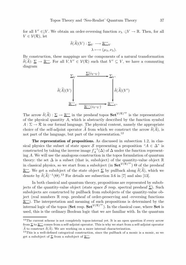
Topos Theory and ‘Neo-Realist’ Quantum Theory 37
for all V ′ ∈↓V . We obtain an order-reversing function νλ :↓V → R. Then, for allV ∈ V(R), let
δ(A)(V ) : ΣV −→ R↔V
λ �−→ (μλ, νλ).
By construction, these mappings are the components of a natural transformationδ(A): Σ → R↔. For all V, V ′ ∈ V(R) such that V ′ ⊆ V , we have a commutingdiagram
R↔V R↔
V ′�R↔(iV ′V )
ΣV ΣV ′�Σ(iV ′V )
�
δ(A)(V )
�
δ(A)(V ′)
The arrow δ(A) : Σ → R↔ in the presheaf topos SetV(R)op
is the representativeof the physical quantity A, which is abstractly described by the function symbolA : Σ →R in our formal language. The physical content, namely the appropriatechoice of the self-adjoint operator A from which we construct the arrow δ(A), isnot part of the language, but part of the representation.12
The representation of propositions. As discussed in subsection 1.2, in clas-sical physics the subset of state space S representing a proposition “A ∈ Δ” isconstructed by taking the inverse image f−1
A (Δ) of Δ under the function represent-ing A. We will use the analogous construction in the topos formulation of quantumtheory: the set Δ is a subset (that is, subobject) of the quantity-value object Rin classical physics, so we start from a subobject (in SetV(R)op
) Θ of the presheafR↔. We get a subobject of the state object Σ by pullback along δ(A), which wedenote by δ(A)−1(Θ).13 For details see subsection 3.6 in [7] and also [13].
In both classical and quantum theory, propositions are represented by subob-jects of the quantity-value object (state space S resp. spectral presheaf Σ). Suchsubobjects are constructed by pullback from subobjects of the quantity-value ob-ject (real numbers R resp. presheaf of order-preserving and -reversing functionsR↔). The interpretation and meaning of such propositions is determined by theinternal logic of the topos (Set resp. SetV(R)op
). In the classical case, where Set isused, this is the ordinary Boolean logic that we are familiar with. In the quantum
12The current scheme is not completely topos-internal yet. It is an open question if every arrowfrom Σ to R↔ comes from a self-adjoint operator. This is why we start from a self-adjoint operator
A to construct δ(A). We are working on a more internal characterization.13This is a well-defined categorical construction, since the pullback of a monic is a monic, so weget a subobject of Σ from a subobject of R↔.

38 Andreas Doring
case, the internal logic of the presheaf topos SetV(R)op
has to be used. This in-tuitionistic logic can be interpreted using Kripke-Joyal semantics, see e.g. chapterVI in [27].
The Heyting algebra structure of subobjects. In the next section, we discussthe representation of states in the topos SetV(R)op
and the assignment of truth-values to propositions. Before doing so, it is worth noting that the subobjects ofΣ form a Heyting algebra (since the subobjects of any object in a topos do), sowe have mapped propositions “A ∈ Δ” (understood as discussed) to a distributivelattice with a pseudocomplement. Together with the results from the next section,we have a completely new form of quantum logic, based upon the internal logicof the presheaf topos SetV(R)op
. Since this is a distributive logic and since theinternal logic of a topos has powerful rules of inference, this kind of quantum logic ispotentially much better interpretable than ordinary quantum logic of the Birkhoff-von Neumann kind. The latter type of quantum logic and its generalizations arebased on nondistributive structures and lack a deductive system.
5. Truth objects and truth-values
In classical physics, a state is just a point of state space.14 Since, as we saw, thespectral presheaf Σ has no elements (or, global elements15), we must representstates differently in the presheaf topos SetV(R)op
.
5.1. Generalized elements as generalized states
One direct way, suggested in [13], is the following generalization: Σ has no globalelements 1 → Σ, but it does have subobjects U ↪→ Σ. In algebraic geometry andmore generally in category theory, such monics (and, more generally, arbitraryarrows) are called generalized elements [25]. We could postulate that these sub-objects, or some of them, are ‘generalized states’. Consider another subobject ofΣ that represents a proposition “A ∈ Δ” about the quantum system, given by itscharacteristic arrow χS : Σ → Ω. Then we can compose these arrows
U ↪→ Σ → Ω
to obtain an arrow U → Ω. This is not a global element 1 → Ω of Ω, and byconstruction, it cannot be, since Σ has no global elements, but it is a generalizedelement of Ω. It might be possible to give a physical meaning to these arrows
14One might call this a pure state, though this is not customary in classical physics. Such a stateactually is a point measure on state space, in contrast to more general probability measures thatdescribe general states. We only consider pure states here and identify the point measure withthe corresponding point of state space.15Elements 1 → P of a presheaf P are called global elements or global sections in category theory.We follow this convention to avoid confusion with points or elements of sets.

Topos Theory and ‘Neo-Realist’ Quantum Theory 39
U → Ω if one can (a) give physical meaning to the subobject U ↪→ Σ, makingclear what a generalized state actually is, and (b) give a logical and physicalinterpretation of an arrow U → Ω. While a global element 1 → Ω is interpreted asa truth-value in the internal logic of a topos, the logical interpretation of an arrowU → Ω is not so clear.
We want to emphasize that mathematically, the above construction is per-fectly well-defined. It remains to be worked out if a physical and logical meaningcan be attached to it.
5.2. The construction of truth objects
We now turn to the construction of so-called ‘truth objects’ from pure quantumstates ψ, see also [6]. (To be precise, a unit vector ψ in the Hilbert space Hrepresents a vector state ϕψ : R → C on a von Neumann algebra, given byϕψ(A) := 〈ψ| A |ψ〉 for all A ∈ R. If R = B(H), then every ϕψ is a pure state.)Of course, the Hilbert space H is the Hilbert space on which the von Neumannalgebra of observables R ⊆ B(H) is represented. This is the most direct wayin which Hilbert space actually enters the mathematical constructions inside thetopos SetV(R)op
. However, we will see how this direct appeal to Hilbert spacepossibly can be circumvented.
Given a subobject of Σ that represents some proposition, a truth object willallow us to construct a global element 1 → Σ of Σ, as we will show in subsection 5.4.This means that from a proposition and a state, we do get an actual truth-valuefor that proposition in the internal logic of the topos SetV(R)op
. The constructionof truth objects is a direct generalization of the classical case.
For the moment, let us consider sets. Let S be a subset of some larger set X ,and let x ∈ X . Then
(x ∈ S) ⇔ (S ∈ U(x)),
where U(x) denotes the set of neighborhoods of x in X . The key observation is thatwhile the l.h.s. cannot be generalized to the topos setting, since we cannot talkabout points like x, the r.h.s. can. The task is to define neighborhoods in a suitablemanner. We observe that U(x) is a subset of the power set PX = P (X), which isthe same as an element of the power set of the power set PPX = P (P (X)).
This leads to the idea that for each context V ∈ V(R), we must choose anappropriate set of subsets of the Gel’fand spectrum ΣV such that these sets ofsubsets form an element in PPΣ. Additionally, the subsets we choose at eachstage V should be clopen, since the clopen subsets Pcl(ΣV ) form a lattice that isisomorphic to the lattice P(V ) of projections in V . If P ∈ V is a projection, thenthe corresponding clopen subset of ΣV is
SP := {λ ∈ ΣV | λ(P ) = 1}.
40 Andreas Doring
Conversely, given a clopen subset S ∈ Pcl(ΣV ), we denote the corresponding pro-jection in P(V ) by PS . It is given as the inverse Gel’fand transform of the charac-teristic function of S.
The main difficulty lies in the fact that the spectral presheaf Σ has no globalelements, which is equivalent to the Kochen-Specker theorem. A global element, ifit existed, would pick one point λV from each Gel’fand spectrum ΣV (V ∈ V(R))such that, whenever V ′ ⊂ V , we would have λV ′ = λV |V ′ . If we had such globalelements, we could define neighborhoods for them by taking, for each V ∈ V(R),neighborhoods of λV in ΣV .
Since no such global elements exist, we cannot expect to have neighborhoodsof points at each stage. Rather, we will get neighborhoods of sets at each stage V ,and only for particular V , these sets will have just one element. In any case, thesets will depend on the state ψ in a straightforward manner. We define:
Definition 4. Let ψ ∈ H be a unit vector, let Pψ the projection onto the corre-sponding one-dimensional subspace (i.e., ray) of H, and let Pcl(ΣV ) be the clopensubsets of the Gel’fand spectrum ΣV . If S ∈ Pcl(ΣV ), then PS ∈ P(V ) denotes thecorresponding projection. The truth object Tψ = (Tψ
V )V ∈V(R) is given by
∀V ∈ V(R) : TψV := {S ∈ Pcl(ΣV ) | 〈ψ| PS |ψ〉 = 1}.
At each stage V , TψV collects all subsets S of ΣV such that the expectation
value of the projection corresponding to this subset is 1. From this definition, it isnot clear at first sight that the set Tψ
V can be seen as a set of neighborhoods.
Lemma 5. We have the following equalities:
∀V ∈ V(R) : TψV = {S ∈ Pcl(ΣV ) | 〈ψ| PS |ψ〉 = 1}
= {S ∈ Pcl(ΣV ) | PS ≥ Pψ}= {S ∈ Pcl(ΣV ) | PS ≥ δo(Pψ)V }= {S ∈ Pcl(ΣV ) | S ⊇ Sδo(Pψ)V
}.
Proof. If 〈ψ| PS |ψ〉 = 1, then ψ lies entirely in the subspace of Hilbert space thatPS projects onto. This is equivalent to PS ≥ Pψ. Since PS ∈ P(V ) and δo(Pψ)V isthe smallest projection in V that is larger than Pψ,16 we also have PS ≥ δo(Pψ)V .In the last step, we simply go from the projections in V to the correspondingclopen subsets of ΣV . �
This reformulation shows that TψV actually consists of subsets of the Gel’fand
spectrum ΣV that can be seen as some kind of neighborhoods, not of a singlepoint of ΣV , but of a certain subset of ΣV , namely Sδo(Pψ)V
. In the simplest case,
16On projections, the spectral order ≤s and the linear order ≤ coincide.

Topos Theory and ‘Neo-Realist’ Quantum Theory 41
we have Pψ ∈ P(V ), so δo(Pψ)V = Pψ . Then Sδo(Pψ)V= SPψ
, and this subsetcontains a single element, namely the pure state λ such that
λ(Pψ) = 1
and λ(Q) = 0 for all Q ∈ P(V ) such that QPψ = 0. In this case, TψV actually
consists of all the clopen neighborhoods of the point λ in ΣV .
In general, if Pψ does not lie in the projections P(V ), then there is no subset ofΣV that corresponds directly to Pψ . We must first approximate Pψ by a projectionin V , and δo(Pψ)V is the smallest projection in V larger than Pψ. The projectionδo(Pψ)V corresponds to a subset Sδo(Pψ)V
⊆ ΣV that may contain more than one
element. However, TψV can still be seen as a set of neighborhoods, but now of this
set Sδo(Pψ)Vrather than of a single point.
It is an interesting and non-trivial point that the (outer) daseinisationδo(Pψ)V (V ∈ V(R)) shows up in this construction. We did not discuss this here,but the subobjects of Σ constructed from the outer daseinisation of projectionsplay a central role in the representation of a certain propositional language PL(S)that one can attach to a physical system S [5, 6]. Moreover, these subobjects are‘optimal’ in the sense that, whenever V ′ ⊂ V , the restriction from Sδo(P )V
toSδo(P )V ′ is surjective, see Theorem 3.1 in [6]. This property can also lead the wayto a more internal characterization of truth-objects, without reference to a stateψ and hence to Hilbert space.
5.3. Truth objects and Birkhoff-von Neumann quantum logic
In this short subsection, we want to consider truth objects from the point of viewof ordinary quantum logic, which goes back to the famous paper [3] by Birkhoffand von Neumann. This is a small digression, since an important part of the toposapproach is to replace ordinary quantum logic by the internal logic of the toposSetV(R)op
. It may still be useful to understand how our constructions relate toBirkhoff-von Neumann quantum logic.
For now, let us assume that R = B(H), then we write P(H) := P(B(H)) forthe lattice of projections on Hilbert space. In their paper, Birkhoff and von Neu-mann identify a proposition “A ∈ Δ” about a quantum system with a projectionoperator E[A ∈ Δ] ∈ P(H) via the spectral theorem [22] and interpret the latticestructure of P(H) as giving a quantum logic. This is very different from the toposform of quantum logic, since P(H) is a non-distributive lattice, leading to all thewell-known interpretational difficulties.
The implication in ordinary quantum logic is given by the partial order onP(H): a proposition “A ∈ Δ1” implies a proposition “B ∈ Δ2” (where we canhave B = A) if and only if E[A ∈ Δ1] ≤ E[B ∈ Δ2] holds for the correspondingprojections.
42 Andreas Doring
The idea now is that, given a pure state ψ and the corresponding projectionPψ onto a ray, we can collect all the projections larger than or equal to Pψ . Wedenote this by
Tψ := {P ∈ P(H) | P ≥ Pψ}.
The propositions represented by these projections are exactly those propositionsabout the quantum system that are (totally) true if the system is in the state ψ.Totally true means ‘true with probability 1’ in an instrumentalist interpretation.If, for example, a projection E[A ∈ Δ] is larger than Pψ and hence contained in Tψ,then, upon measurement of the physical quantity A, we will find the measurementresult to lie in the set Δ with certainty (i.e., with probability 1).
Tψ is a maximal (proper) filter in P(H). Every pure state ψ gives rise to sucha maximal filter Tψ, and clearly, the mapping ψ �→ Tψ is injective. We can obtainthe truth object Tψ from the maximal filter Tψ simply by defining
∀V ∈ V(R) : TψV := Tψ ∩ V.
In each context V , we collect all the projections larger than Pψ . On the levelof propositions, we have all the propositions about physical quantities A in thecontext V that are totally true in the state ψ.
5.4. The assignment of truth-values to propositions
We return to the consideration of the internal logic of the topos SetV(R)op
andshow how to define a global element 1 → Ω of the subobject classifier from a clopensubobject S of Σ and a truth object Tψ . The subobject S represents a propositionabout the quantum system, the truth object Tψ represents a state, and the globalelement of Ω will be interpreted as the truth-value of the proposition in the givenstate. Thus, we make use of the internal logic of the topos SetV(R)op
of presheavesover the context category V(R) to assign truth-values to all propositions about aquantum system.
It is well known that the subobject classifier Ω in a topos of presheaves is thepresheaf of sieves (see e.g. [27]). A sieve σ on an object A in some category C is acollection of arrows with codomain A with the following property: if f : B → A isin σ and g : C → B is another arrow in C, then f ◦ g : C → A is in σ, too. In otherwords, a sieve on A is a downward closed set of arrows with codomain A. Sincethe context category V(R) is a partially ordered set, things become very simple:the only arrows with codomain V are the inclusions iV ′V . Since such an arrow isspecified uniquely by its domain V ′, we can think of the sieve σ on V as consistingof certain subalgebras V ′ of V . If V ′ ∈ σ and V ′′ ⊂ V ′, then V ′′ ∈ σ.
The restriction mappings of the presheaf Ω are given by pullbacks of sieves.The pullback of sieves over a partially ordered set takes a particularly simple form:

Topos Theory and ‘Neo-Realist’ Quantum Theory 43
Lemma 6. If σ is a sieve on V ∈ V(R) and V ′ ⊂ V , then the pullback σ · iV ′V isgiven by σ∩ ↓V ′. (This holds analogously for sieves on any partially ordered set,not just V(R)).
Proof. For the moment, we switch to the arrows notation. By definition, the pull-back σ · iV ′V is given by
σ · iV ′V := {iV ′′V ′ | iV ′V ◦ iV ′′V ′ ∈ σ}.
We now identify arrows and subalgebras as usual and obtain (using the fact thatV ′′ ⊆ V ′ implies V ′′ ⊂ V )
{iV ′′V ′ | iV ′V ◦ iV ′′V ′ ∈ σ} � {V ′′ ⊆ V ′ | V ′′ ∈ σ} =↓V ′ ∩ σ.
Since ↓ V ′ is the maximal sieve on V ′, the pullback σ · iV ′V is given as the inter-section of σ with the maximal sieve on V ′. �
The name �S� of the subobject S is the unique arrow 1 → PΣ = ΩΣ intothe power object of Σ (i.e., the subobjects of Σ) that ‘picks out’ S among allsubobjects. �S� is a global element of PΣ. Here, one uses the fact that powerobjects behave like sets, in particular, they have global elements. Since we assumethat S is a clopen subobject, we also get an arrow 1 → PclΣ into the clopen powerobject of Σ, see [6]. We denote this arrow by �S�, as well.
Since Tψ ∈ PPclΣ is a collection of clopen subobjects of Σ, it makes senseto ask if S is among them; an expression like �S� ∈ Tψ is well-defined. We define,for all V ∈ V(R), the valuation
v(�S� ∈ Tψ)V := {V ′ ⊆ V | S(V ′) ∈ TψV ′}.
At each stage V , we collect all those subalgebras of V such that S(V ′) is containedin Tψ
V ′ .
In order to construct a global element of the presheaf of sieves Ω, we mustfirst show that v(�S� ∈ Tψ)V is a sieve on V . In the proof we use the fact thatthe subobjects obtained from daseinisation are optimal in a certain sense.
Proposition 7. v(�S� ∈ Tψ)V := {V ′ ⊆ V | S(V ′) ∈ TψV ′} is a sieve on V .
Proof. As usual, we identify an inclusion morphism iV ′V with V ′ itself, so a sieve onV consists of certain subalgebras of V . We have to show that if V ′ ∈ v(�S� ∈ Tψ)V
and V ′′ ⊂ V ′, then V ′′ ∈ v(�S� ∈ Tψ)V . Now, V ′ ∈ v(�S� ∈ Tψ)V meansthat S(V ′) ∈ Tψ
V ′ , which is equivalent to S(V ′) ⊇ Sδo(Pψ)V ′ . Here, Sδo(Pψ)V ′is the component at V ′ of the sub-object Sδo(Pψ) = (Sδo(Pψ)V
)V ∈V(R) of Σ ob-
tained from daseinisation of Pψ. According to Thm. 3.1 in [6], the sub-objectSδo(Pψ) is optimal in the following sense: when restricting from V ′ to V ′′, we have

44 Andreas Doring
Σ(iV ′′V ′)(Sδo(Pψ)V ′ ) = Sδo(Pψ)V ′′ , i.e., the restriction is surjective. By assumption,S(V ′) ⊇ Sδo(Pψ)V ′ , which implies
S(V ′′) ⊇ Σ(iV ′′V ′)(S(V ′)) ⊇ Σ(iV ′′V ′)(Sδo(Pψ)V ′ ) = Sδo(Pψ)V ′′ .
This shows that V ′′ ∈ TψV ′′ and hence V ′′ ∈ v(�S� ∈ Tψ)V . �
Finally, we have to show that the sieves v(�S� ∈ Tψ)V , V ∈ V(R), actuallyform a global element of Ω, i.e., they all fit together under the restriction mappingsof the presheaf Ω:
Proposition 8. The sieves v(�S� ∈ Tψ)V , V ∈ V(R), (see Prop. 7) form a globalelement of Ω.
Proof. From Lemma 6, is suffices to show that, whenever V ′ ⊂ V , we have v(�S� ∈Tψ)V ′ = v(�S� ∈ Tψ)V ∩ ↓V ′. If V ′′ ∈ v(�S� ∈ Tψ)V ′ , then S(V ′′) ∈ Tψ
V ′′ , whichimplies V ′′ ∈ v(�S� ∈ Tψ)V . Conversely, if V ′′ ∈↓V ′ and V ′′ ∈ v(�S� ∈ Tψ)V ,then, again, S(V ′′) ∈ Tψ
V ′′ , which implies V ′′ ∈ v(�S� ∈ Tψ)V ′ . �
The global element v(�S� ∈ Tψ) = (v(�S� ∈ Tψ)V )V ∈V(R) of Ω is interpretedas the truth-value of the proposition represented by S ∈ Pcl(Σ) if the quantumsystem is in the state ψ (resp. Tψ). This assignment of truth-values is
• contextual, since the contexts V ∈ V(R) play a central role in the wholeconstruction
• global in the sense that every proposition is assigned a truth-value• completely independent of any notion of measurement or observer, hence we
call our scheme a ‘neo-realist’ formulation of quantum theory• topos-internal, the logical structure is not chosen arbitrarily, but fixed by the
topos SetV(R)op
. This topos is directly motivated from the Kochen-Speckertheorem
• non-Boolean, since there are (a) more truth-values than just ‘true’ and ‘false’and (b) the global elements form a Heyting algebra, not a Boolean algebra.There is a global element 1 of Ω, consisting of the maximal sieve ↓V at eachstage V , which is interpreted as ‘totally true’, and there is a global element0 consisting of the empty sieve for all V , which is interpreted as ‘totallyfalse’. Apart from that, there are many other global elements that representtruth-values between ‘totally true’ and ‘totally false’. These truth-values areneither numbers nor probabilities, but are given by the logical structure ofthe presheaf topos SetV(R)op
. Since the Heyting algebra of global elements ofΩ, i.e., of truth-values, is a partially ordered set only, there are truth-valuesv1, v2 such that neither v1 < v2 nor v2 < v1, which is also different from two-valued Boolean logic where simply 0 < 1 (i.e., ‘false’<‘true’). The presheaftopos SetV(R)op
has a rich logical structure.
Topos Theory and ‘Neo-Realist’ Quantum Theory 45
6. Conclusion and outlook
The formulation of quantum theory within the presheaf topos SetV(R)op
gives atheory that is remarkably similar to classical physics from a structural perspective.In particular, there is a state object (the spectral presheaf Σ) and a quantity-valueobject (the presheaf R↔ of order-preserving and -reversing functions). Physicalquantities are represented by arrows between Σ and R↔.
One of the future tasks will be the incorporation of dynamics. The processof daseinisation behaves well with respect to the action of unitary operators, seesection 5.2 in [7], so it is conceivable that there is a ‘Heisenberg picture’ of dy-namics. Commutators remain to be understood in the topos picture. On the otherhand, it is possible to let a truth-object Tψ change in time by applying Schrodingerevolution to ψ. It remains to be shown how this can be understood topos-internally.
Mulvey and Banaschewski have recently shown how to define the Gel’fandspectrum of an abelian C∗-algebra A in any Grothendieck topos, using constructivemethods (see [2] and references therein). Spitters and Heunen made the followingconstruction in [13]: one takes a non-abelian C∗-algebra A and considers the toposof (covariant) functors over the category of abelian subalgebras of A. The algebraA induces an internal abelian C∗-algebra A in this topos of functors. (Internally,algebraic operations are only allowed between commuting operators.) Spitters andHeunen observed that the Gel’fand spectrum of this internal algebra basically isthe spectral presheaf.17 It is very reassuring that the spectral presheaf not onlyhas a physical interpretation, but also such a nice and natural mathematical one.Spitters and Heunen also discuss integration theory in the constructive context.These tools will be very useful in order to regain actual numbers and expectationvalues from the topos formalism.
Since the whole topos programme is based on the representation of formallanguages, major generalizations are possible. One can represent the same lan-guage L(S) in different topoi, as we already did with Set for classical physics andSetV(R)op
for algebraic quantum theory. For physical theories going beyond this,other topoi will play a role. The biggest task is the incorporation of space-timeconcepts, which will, at the very least, necessitate a change of the base category.It is also conceivable that the ‘smooth topoi’ of synthetic differential geometry(SDG) will play a role.
Acknowledgements
I want to thank Chris Isham for numerous discussions and constant support. More-over, I would like to thank Bob Coecke, Samson Abramsky, Jamie Vicary, Bas
17The change from presheaves, i.e., contravariant functors, to covariant functors is necessary inthe constructive context.

46 Andreas Doring
Spitters and Chris Heunen for stimulating discussions. This work was supportedby the DAAD and the FQXi, which is gratefully acknowledged. Finally, I want tothank the organizers of the RDQFT workshop, Bertfried Fauser, Jurgen Tolksdorfand Eberhard Zeidler, for inviting me. It was a very enjoyable experience.
References
[1] J. L. Bell, Toposes and Local Set Theories (Clarendon Press, Oxford 1988)
[2] B. Banaschewski, C. J. Mulvey, “A globalisation of the Gelfand duality theorem”,Ann. of Pure and Applied Logic 137 (2006), 62-103
[3] G. Birkhoff, J. von Neumann, “The logic of quantum mechanics”, Ann. of Math. 37(1936), 823-843
[4] A. Doring, “Kochen-Specker Theorem for von Neumann Algebras”, Int. J. Theor.Phys. 44, no. 2 (2005), 139-160
[5] A. Doring, C. J. Isham, “A Topos Foundation for Theories of Physics: I. FormalLanguages for Physics”, quant-ph/0703060, to appear in J. Math. Phys. (March2008)
[6] A. Doring, C. J. Isham, “A Topos Foundation for Theories of Physics: II. Daseini-sation and the Liberation of Quantum Theory”, quant-ph/0703062, to appear in J.Math. Phys. (March 2008)
[7] A. Doring, C. J. Isham, “A Topos Foundation for Theories of Physics: III. The Rep-
resentation of Physical Quantities with Arrows δo(A) : Σ → R�”, quant-ph/0703064,to appear in J. Math. Phys. (March 2008)
[8] A. Doring, C. J. Isham, “A Topos Foundation for Theories of Physics: IV. Categoriesof Systems”, quant-ph/0703066, to appear in J. Math. Phys. (March 2008)
[9] R. Goldblatt, Topoi, The Categorical Analysis of Logic, revised second edition(North-Holland, Amsterdam, New York, Oxford 1984)
[10] H. F. de Groote, “On a canonical lattice structure on the effect algebra of a vonNeumann algebra”, quant-ph/0410018 v2 (2005)
[11] H. F. de Groote, “Observables”, math-ph/0507019
[12] H. F. de Groote, “Observables IV: The Presheaf Perspective”, math-ph/0708.0677
[13] C. Heunen, B. Spitters, “A topos for algebraic quantum theory”, quant-ph/0709.4364
[14] C. J. Isham “Topos Theory and Consistent Histories: The Internal Logic of the Setof all Consistent Sets”, Int. J. Theor. Phys. 36 (1997), 785-814
[15] C. J. Isham, J. Butterfield, “A topos perspective on the Kochen-Specker theorem: I.Quantum states as generalised valuations”, Int. J. Theor. Phys. 37 (1998), 2669-2733
[16] C. J. Isham, J. Butterfield, “A topos perspective on the Kochen-Specker theorem: II.Conceptual aspects, and classical analogues”, Int. J. Theor. Phys. 38 (1999), 827-859
[17] C. J. Isham, J. Butterfield, “Some Possible Roles for Topos Theory in QuantumTheory and Quantum Gravity”, Found. Phys. 30 (2000), 1707-1735
[18] C. J. Isham, J. Butterfield, J. Hamilton, “A topos perspective on the Kochen-Speckertheorem: III. Von Neumann algebras as the base category”, Int. J. Theor. Phys. 39(2000), 1413-1436

Topos Theory and ‘Neo-Realist’ Quantum Theory 47
[19] C. J. Isham, J. Butterfield, “A topos perspective on the Kochen-Specker theorem:IV. Interval valuations”, Int. J. Theor. Phys. 41, no. 4 (2002), 613-639
[20] P. T. Johnstone, Sketches of an Elephant, A Topos Theory Compendium, Vol. 1(Clarendon Press, Oxford 2002)
[21] P. T. Johnstone, Sketches of an Elephant, A Topos Theory Compendium, Vol. 2(Clarendon Press, Oxford 2002)
[22] R. V. Kadison, J. R. Ringrose, Fundamentals of the Theory of Operator Algebras,Vol. 1 (Academic Press, San Diego 1983; AMS reprint 2000)
[23] S. Kochen, E. P. Specker, “The problem of hidden variables in quantum mechanics”,Journal of Mathematics and Mechanics 17 (1967), 59-87
[24] J. Lambek, P. J. Scott, Introduction to higher order categorical logic (CambridgeUniversity Press, Cambridge, New York etc. 1986)
[25] F. W. Lawvere, R. Rosebrugh, Sets for Mathematics (Cambridge University Press,Cambridge 2003)
[26] S. Mac Lane, Categories for the Working Mathematician (Springer, New York,Berlin etc. 1971; second, revised edition 1997)
[27] S. Mac Lane, I. Moerdijk, Sheaves in Geometry and Logic, A First Introduction toTopos Theory, Springer (New York, Berlin etc. 1992)
[28] M. P. Olson, “The Selfadjoint Operators of a von Neumann Algebra Form a Condi-tionally Complete Lattice”, Proc. of the AMS 28 (1971), 537-544
[29] M. H. Stone, “The theory of representations for Boolean algebras”, Trans. Amer.Math. Soc. 40 (1936), 37-111
Andreas DoringTheoretical Physics GroupBlackett LaboratoryImperial College of Science, Technology & MedicinePrince Consort RoadSouth KensingtonLondon SW7 2BZ
e-mail: [email protected]


Quantum Field TheoryB. Fauser, J. Tolksdorf and E. Zeidler, Eds., 49–66c© 2009 Birkhauser Verlag Basel/Switzerland
A Survey on Mathematical Feynman PathIntegrals: Construction, Asymptotics,Applications
Sergio Albeverio and Sonia Mazzucchi
Abstract. Theory and main applications of infinite dimensional oscillatoryintegrals are discussed, with special attention to the mathematical realizationof Feynman path integrals
Mathematics Subject Classification (2000). Primary 28C20; Secondary 35Q40;46F20; 60G60; 81S40; 81T10; 81T45; 81P15; 35C20.
Keywords. oscillatory integrals, Feynman path integrals, stationary phase,polynomial potentials, semiclassical expansions, trace formula, Chern-Simonsmodel.
1. Introduction
The study of oscillatory integrals of the form
IΦε (f) = “
∫RN
eiΦε (x)f(x)dx
′′(1)
is a classical topic, largely developed in connections with several applications inmathematics, such as the theory of Fourier integral operators [51, 66], and inphysics (for instance in optics, see, e.g., [26]). In the expression on the right handside of (1) Φ denotes a real valued “phase function”, f a complex valued functionand ε ∈ R+ a real parameter. Well known examples of integrals of the form (1)are the Fresnel integrals ∫
R
eix2f(x)dx
applied in the theory of wave diffraction and the Airy integrals∫R
eix3f(x)dx

50 Sergio Albeverio and Sonia Mazzucchi
applied in the theory of the rainbow. The fundamental feature of the integral (1)is the oscillatory behavior of the term eiΦ
ε , which allows to define the integralas an improper Riemann integral even if the function f is not summable, byexploiting the cancelations due to the alternating of the sign of the integrand. Thisproperty makes oscillatory integrals the suitable mathematical objects representingthe physical concept of coherent superposition, that is of interference. It is thus notsurprising that, besides optics, electromagnetism and hydrodynamics, one of themost suggestive and powerful applications of oscillatory integrals can be found innon relativistic quantum mechanics. Indeed in 1942 R. Feynman [38], inspired bya paper by Dirac [35], proposed an alternative formulation of quantum mechanicsusing heuristic infinite dimensional oscillatory integrals. According to Feynman thesolution of the Schrodinger equation, describing the time evolution of the state ofa quantum particle moving under the influence of a (real-valued) potential V{
i� ∂∂tψ = − �2
2mΔψ + V ψψ(0, x) = ψ0(x)
(2)
(m denotes the mass of the particle and � the reduced Planck constant), should begiven by a “sum over all possible histories”. In other words the wave function ofthe system at time t evaluated at the point x ∈ Rd should be given by an integralon the space of continuous paths γ ending at time t at the point x:
ψ(t, x) = “
∫{γ|γ(t)=x}
ei�
St(γ)ψ0(γ(0))Dγ′′. (3)
St(γ) is the classical action of the system evaluated along the path γ
St(γ) = S0(γ)−∫ t
0
V (s, γ(s))ds, S0(γ) =m
2
∫ t
0
|γ(s)|2ds
and Dγ denotes a heuristic “flat” measure on the space of paths. The heuristicexpression (3) can be regarded as an infinite dimensional analogue of the integral(1):
IΦε = “
∫Γ
eiΦε (γ)f(γ)dγ
′′, (4)
that is an oscillatory integral on an (infinite dimensional) space of paths Γ withε = �. The Feynman path integral approach of quantum mechanics is particularlysuggestive as it creates a connection between the classical Lagrangian descriptionof the physical world and the quantum one, reintroducing in quantum mechanicsthe concept of trajectory, which had been banned by the traditional formulationof quantum theory. Formula (3) provides a quantization method allowing, at leastheuristically, to associate to each classical Lagrangian a quantum evolution. Feyn-man himself extended the path integral approach to the description of the dynam-ics of more general quantum systems, including the quantum fields, and producinga heuristic calculus that, from a physical point of view, often works even in caseswhere other methods fail.

A Survey of Feynman Path Integrals 51
Another feature of oscillatory integrals which makes representation (3) par-ticularly interesting is the existence of a well known theory allowing one to studythe asymptotic behavior of integrals (1) when ε is regarded as a small parame-ter converging to 0. Originally introduced by Stokes and Kelvin and successivelydeveloped by several mathematicians, in particular van der Corput (who, by theway, was particularly interested in applications to number theory), the “stationaryphase method” provides a powerful tool to handle the asymptotics of (1) as ε ↓ 0.According to it, the main contribution to the asymptotic behavior of the integralshould come from those points x ∈ RN belonging to the critical manifold:
{x ∈ RN , | Φ′(x) = 0},that is the points which make stationary the phase function Φ. The asymptoticanalysis of oscillatory integrals is successfully applied to different areas of mathe-matics such as the theory of (partial) differential equations, the singularity theoryand the number theory.
The extension of these techniques to the infinite dimensional case and inparticular to the Feynman formula (3) makes very intuitive the study of the semi-classical limit of quantum mechanics, that is the study of the detailed behavior ofthe wave function ψ in the case the Planck constant � is regarded as a small pa-rameter. According to an (heuristic) application of the stationary phase method,in the limit � ↓ 0 the main contribution to the integral (3) should come fromthose paths γ which make stationary the action functional St. These, by Hamil-ton’s least action principle, are exactly the classical orbits of the system. Moreoverthe heuristic applications of the asymptotic expansion of Feynman path integrals(and related Euclidean path integrals) in quantum field theory gives interestingresults connected to the study of solitons resp. instantons, resp. in the case ofcertain gauge fields, of topological invariants (see, e.g., [73, 74, 59, 68] for physicaldiscussion and e.g. , [76], [41] and [3] for Euclidean path integrals).
Despite its fascinating features, formula (3) lacks of mathematical rigor, in-deed the Lebesgue “flat” measure Dγ on the space on paths does not have amathematical meaning (it is quite simple to see that on an infinite dimensionalHilbert space it is not possible to construct a Lebesgue-type measure, that is aσ−additive regular measure which is invariant by translations and rotations andsuch that the measure of bounded open sets is strictly positive and finite). Feyn-man himself was aware of this problem as he writes “one must feel as Cavalierimust have felt calculating the volume of a pyramid before the invention of thecalculus”. The challenge to give meaning to Feynman’s heuristic calculus and todefine rigorously oscillatory integrals (4) in infinite dimension, as well as to de-velop an infinite dimensional version of the stationary phase method, was left tomathematicians (see also, e.g. [3, 50, 58]).
The difficulties are twofold:• First of all one has to define an integration theory on a space of paths, that is
on an infinite dimensional space. We recall that integration theory in spacesof continuous functions was present at Feynman’s time thanks in particular

52 Sergio Albeverio and Sonia Mazzucchi
to the work by Wiener on Brownian motion in the 20’s (particularly in 1923)and much successive work by Cameron, Martin and others giving rise to thetheory of stochastic processes, see e.g.[3]. However there is no mention ofWiener integrals in Feynman’s papers.
• In the definition of Feynman path integrals one should exploit the oscillatorybehavior of the integrand. In principle the convergence of the integral shouldbe given by the cancelations due to this oscillatory behavior.In the next section we shall briefly describe a solution of this problem, while
in section 3 several interesting applications of Feynman path integrals to quantummechanics and quantum fields will be mentioned. Due to limitation of space andtime, we will mainly concentrate on lines of research directly connected to our ownones and with recent developments. In particular some very interesting topics haveto be left out, e.g. extensions to Dirac systems see, e.g. [54, 55], hyperbolic systems[78], oscillatory complex Gaussian integrals, see also e.g., the extensive referencesin [3, 12, 58, 61].
2. The mathematical realization of Feynman path integrals
In this section we shall see how the definition and the main properties of classicaloscillatory integrals in finite dimension can be extended to the case where theintegration is performed on an infinite dimensional Hilbert space.
A systematic treatment of finite dimensional oscillatory integrals, as well astheir application to the theory of Fourier integral operators, can be found in thework by Hormander [51] (see also, e.g., [36] and [66]). According to Hormander,the integral (1) can be computed even when the function f is not summable byexploiting the cancelations due to the oscillatory behavior of the integrand. Theoscillatory integral is defined as the limit of a sequence of regularized integrals.
Definition 1. Let f : Rn → C be a Borel function and Φ : Rn → R a phasefunction. If for each test function φ ∈ S(Rn) such that φ(0) = 1 the integrals
Iδ(f, φ) :=∫
Rn
(2πiε)−n/2eiΦ(x)ε f(x)φ(δx)dx
exist for all δ > 0 and limδ→0 Iδ(f, φ) exists and is independent of φ, then the limitis called the oscillatory integral of f with respect to Φ
ε and denoted by∫Rn
eiΦ(x)ε f(x)dx ≡ I
Φε (f). (5)
In the special case where the phase function is a quadratic form, the oscilla-tory integral is called Fresnel integral (following the name given to certain integralsin optics, see [12]).
The existence of the integral IΦε (f) can be proved for large classes of functions
Φ, f [51, 52, 36, 66, 17], even though a complete direct characterization of the classfor which the integral is well defined is still an open problem. However, for suitable
A Survey of Feynman Path Integrals 53
Φ, it is possible to find an interesting set of “integrable functions”, for which theoscillatory integral IΦ(f) can be explicitly computed in terms of an absolutelyconvergent integral thanks to a Parseval-type equality.
Given a (finite or infinite dimensional) real separable Hilbert space (H, 〈 , 〉),whose elements are
denoted by x, y ∈ H, let us denote by F(H) the space of complex functionson H which are Fourier transforms of complex bounded variation measures on H:
f ∈ F(H), f(x) =∫Hei〈x,y〉dμf (y).
F(H) is a Banach algebra of functions, where the product is the pointwise one,the unit element is the function identically one 1, i.e. 1(x) = 1 ∀x ∈ H and thenorm of a function f is given by the total variation of the corresponding measureμf :
‖f‖F(H) = ‖μf‖ = sup∑
i
|μ(Ei)|,
where the supremum is taken over all sequences {Ei} of pairwise disjoint Borelsubsets of H, such that ∪iEi = H. It is possible to prove [17] that if f ∈ F(Rn),
f = μf , and for phase functions Φ such that FΦ ≡ ei Φε
(2πiε)n/2 has a Fourier transform
FΦ which is integrable (in Lebesgue sense) with respect to μf , then the oscillatoryintegral IΦ(f) exists and it is given by the following “Parseval formula”:
IΦ(f) =∫
Rn
FΦ(α)dμf (α). (6)
Equation (6) holds for smooth phase functions Φ of at most even polynomialgrowth at infinity.Equation (6) allows, in the case Φ is an homogeneous polynomial and under regu-larity assumptions on the function f , to compute (see [17]) the detailed asymptoticexpansion of the integral I
Φ� (f) in fractional powers of the parameters � around
a degenerate (or non degenerate) critical point, with a strong control on the re-mainders. The study of the asymptotics of oscillatory integrals in the case wherethe critical manifold contains degenerate critical points is related with singularitytheory and catastrophe theory [27, 36, 26].
The generalization of these results to the infinite dimensional case involvesseveral technical difficulties. Indeed in the 60’s Cameron [28] proved that it is notpossible to realize the heuristic Feynman measure
dμF (γ) ≡ ei�
S0(γ)Dγ∫e
i�
S0(γ)Dγ
as a complex measure on the space of paths, as it would have infinite total vari-ation (even locally). This means that for Feynman integrals it is not possible toimplement an integration theory in the traditional Lebesgue sense.

54 Sergio Albeverio and Sonia Mazzucchi
The main idea to overcome this problem is dualization. In other words theintegral
“∫
f(γ)e
i�
S0(γ)Dγ∫e
i�
S0(γ)Dγ
′′= “
∫f(γ)dμF (γ)′′ := IF (f)
has to be realized as a linear continuous functional on a suitable topological algebraof “integrable functions”, generalizing the idea of (Radon) measure as linear func-tional on the space of bounded continuous functions (on locally compact spaces).Among the different approaches to the mathematical definition of the “Feynmanfunctional”, the most implemented are the theory of infinite dimensional oscilla-tory integrals on Hilbert (resp. Banach spaces) [12] and the white noise calculus[50]. In the following we shall extensively describe the first approach and give someelements of the latter.
Let us denote by (H, 〈 , 〉) an infinite dimensional real separable Hilbertspace, Φ : H → R a phase function and f : H → C a complex valued function. Aninfinite dimensional oscillatory integral on the Hilbert space H can be defined asthe limit of a sequence of finite dimensional approximations, as proposed in [37, 7].
Definition 2. A function f : H → C is said to be integrable with respect to thephase function Φ : H → R if for any sequence Pn of projectors onto n-dimensionalsubspaces of H, such that Pn ≤ Pn+1 and Pn → 1 strongly as n→∞ (1 being theidentity operator in H), the finite dimensional approximations∫
PnHeiΦ(Pnx)
ε f(Pnx)d(Pnx),
are well defined (in the sense of definition 1) and the limit
limn→∞
∫PnH
eiΦ(Pnx)ε f(Pnx)d(Pnx) (7)
exists and is independent of the sequence {Pn}.In this case the limit is called oscillatory integral of f with respect to the phasefunction Φ and is denoted by
IΦ(f) ≡∫HeiΦ(x)
ε f(x)dx.
As in the finite dimensional case, the basic question is the characterizationof the class of functions f and Φ for which the integral IΦ(f) is well defined.According to [12, 37, 7], in the case where f belongs to the Banach algebra F(H)of C−valued functions on H which are Fourier transform of bounded complexmeasures on H and Φ is of the form Φ = Φ0 + V , where Φ0 is a quadratic formand V ∈ F(H), then IΦ(f) can be explicitly computed in terms of a Parseval typeequality. In the following the small parameter ε will be replaced by � because ofits meaning in the applications to quantum mechanics.
A Survey of Feynman Path Integrals 55
Theorem 1. Let L : H → H be a self adjoint trace class operator, such that I − Lis invertible. Let f, V ∈ F(H). Let us consider the phase function Φ : H → C,given by
Φ(x) = Φ0(x) + V (x), x ∈ H (8)
with Φ0(x) = 〈x,(I−L)x〉2 . Then the infinite dimensional oscillatory integral IΦ(f)
is well defined and it is given by∫He
i�Φ(x)f(x)dx =
∫He
i2�
〈x,(I−L)x〉− i�
V (x)f(x)dx
= (det(I − L))−1/2
∫He−
i�
2 〈x,(I−L)−1x〉μfe− i
�V (dx).
det(I−L) is the Fredholm determinant of the operator (I−L) (that is the productof the eigenvalues of I − L). The right hand side is explicitly computable (e.g. byan expansion in powers of e−
i�
V ) as fe−i�
V ∈ F(H).
This result has been recently generalized [18] to phase functions of the form
Φ(x) = Φ0(x) + λP (x), x ∈ H, (9)
where Φ0 is of the type handled in theorem 1, λ ∈ R+ and P is a fourth orderpolynomial. In this case the integral IΦ(f), f ∈ F(H), is still computable in termsof a Parseval type equality:
IΦ(f) =∫He
i�Φ(x)f(x)dx =
∫HFΦ(x)dμf (x) (10)
with FΦ defined by
FΦ(x) = limn→∞(2πi�)−n/2
∫PnH
ei〈Pnx,Pny〉ei�Φ(Pny)dPny
= E[eiei π4√
�〈x, · 〉e12 〈 · ,L · 〉e−iλ�P ( · )] (11)
where the expectation is taken with respect to N(0, IH), the centered standardGaussian measure associated with H. Analogously one has
IΦ(f) = E[f(ei π4√
� · )e 12 〈 · ,L · 〉e−iλ�P ( · )]. (12)
It is possible to prove that the right hand side of (12) is an analytic function forIm(λ) < 0 and continuous for Im(λ) = 0. Moreover a corresponding result can beproved for Φ = Φ0 + λP + V , with V ∈ F(H).
The infinite dimensional oscillatory integrals have some interesting proper-ties, which are important as they mirror some heuristic features of formal Feynmanpath integrals, in the case where the Hilbert space H is a space of paths γ. First ofall they have simple transformation properties under “translations and rotations”in paths space, reflecting the fact that dx should represent a flat measure. Theysatisfy a Fubini-type theorem, concerning iterated integration in paths space, al-lowing, in the physical applications, to construct a one parameter group of unitaryoperators associated to the time evolution described by the Schrodinger equation.

56 Sergio Albeverio and Sonia Mazzucchi
They can be approximated by finite dimensional oscillatory integrals, allowing asequential (“time slicing”) approach very close to Feynman’s original derivation.They are also related, via the Parseval type equality (12), to (Gaussian) proba-bilistic integrals, allowing an “analytic continuation approach” (largely developedby several authors [28, 29, 56, 57, 58, 69, 14, 8, 79]).
Moreover, the functional IΦ(f) satisfies a “duality property”, in other wordsthe application
f ∈ F(H) �→ IΦ(f)
is continuous in the norm of the Banach algebra F(H). The duality property iscentral also in other approaches, e.g. [30] and [15]. It is also the main idea of thewhite noise calculus approach [50], where the Feynman functional IΦ(f) is realizedas the pairing between the function f and an infinite dimensional distribution TΦ
(in the framework of the Hida calculus):
IΦ(f) = (S′)〈TΦ, f〉(S)
where the Gelfand triple is
(S) ⊂ L2(S′(Rs), N(0, IL2(Rs)) ⊂ (S′),
N(0, IL2(Rs)) being the Gaussian white noise measure, (S) = (S(Rs)) being essen-tially an infinite dimensional analogue of S(Rs) ⊂ L2(Rs), and correspondingly(S′) = (S′(Rs)) an infinite dimensional analogue of S′(Rs), the space of tempereddistributions.
It is worthwhile to underline that, within all the approaches, the phase func-tion Φ which can be handled are essentially of the form (8), except for the pos-sibility of including functions V of the form of a Laplace transform of boundedmeasures, and some singular V , see, for example [12, 15, 50, 63]. The only approachwhich is able to handle a (quartic) polynomial term as in (9) and the correspond-ing method of stationary phase seems to be the infinite dimensional oscillatoryintegrals approach described above.
3. Applications
3.1. Quantum mechanics
The first application of the infinite dimensional oscillatory integrals is the math-ematical realization of the Feynman path integral representation for the solutionof the Schrodinger equation. Let us consider the Cameron-Martin space Ht, thatis the Hilbert space of absolutely continuous paths γ : [0, t] → Rd with γ(t) = 0and square integrable weak derivative
∫ t
0 γ(s)2ds < ∞, endowed with the innerproduct
〈γ1, γ2〉 =∫ t
0
γ1(s) · γ2(s)ds.
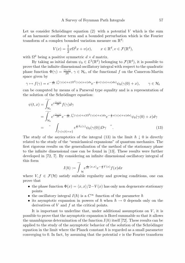
A Survey of Feynman Path Integrals 57
Let us consider Schrodinger equation (2) with a potential V which is the sumof an harmonic oscillator term and a bounded perturbation which is the Fouriertransform of a complex bounded variation measure on Rd:
V (x) =12xΩ2x + v(x), x ∈ Rd, v ∈ F(Rd),
with Ω2 being a positive symmetric d× d matrix.By taking as initial datum ψ0 ∈ L2(Rd) belonging to F(Rd), it is possible to
prove that the infinite dimensional oscillatory integral with respect to the quadraticphase function Φ(γ) = 〈γ,γ〉
2� , γ ∈ Ht, of the functional f on the Cameron-Martinspace given by
γ �→ f(γ) = e−i
2�
∫t0 (γ(s)+x)Ω2(γ(s)+x)dse−
i�
v(γ(s)+x)ds)ψ0(γ(0) + x), γ ∈ Ht
can be computed by means of a Parseval type equality and is a representation ofthe solution of the Schrodinger equation:
ψ(t, x) =∫Ht
ei 〈γ,γ〉2� f(γ)dγ
=∫Ht
ei 〈γ,γ〉2� e−
i2�
∫ t0 (γ(s)+x)Ω2(γ(s)+x)dse−
i�
v(γ(s)+x)ds)ψ0(γ(0) + x)dγ
= “
∫{γ|γ(t)=x}
ei�
St(γ)ψ0(γ(0))Dγ′′. (13)
The study of the asymptotics of the integral (13) in the limit � ↓ 0 is directlyrelated to the study of the “semiclassical expansions” of quantum mechanics. Thefirst rigorous results on the generalization of the method of the stationary phaseto the infinite dimensional case can be found in [13]. These results were furtherdeveloped in [72, 7]. By considering an infinite dimensional oscillatory integral ofthis form
I(�) :=∫
He
i2�
〈x,x〉e−i�
V (x)f(x)dx
where V, f ∈ F(H) satisfy suitable regularity and growing conditions, one canprove that• the phase function Φ(x) = 〈x, x〉/2−V (x) has only non degenerate stationary
points• the oscillatory integral I(�) is a C∞ function of the parameter �• its asymptotic expansion in powers of � when � → 0 depends only on the
derivatives of V and f at the critical points.It is important to underline that, under additional assumptions on V , it is
possible to prove that the asymptotic expansion is Borel summable so that it allowsthe unambiguous determination of the function I(�) itself [72]. These results can beapplied to the study of the asymptotic behavior of the solution of the Schrodingerequation in the limit where the Planck constant � is regarded as a small parameterconverging to 0. In fact, by assuming that the potential v is the Fourier transform
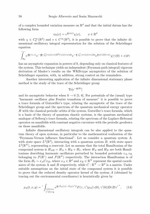
58 Sergio Albeverio and Sonia Mazzucchi
of a complex bounded variation measure on Rd and that the initial datum has thefollowing form
ψ0(x) = ei�
s(x)χ(x), x ∈ Rd
with χ ∈ C∞0 (Rd) and s ∈ C∞(Rd), it is possible to prove that the infinite di-
mensional oscillatory integral representation for the solution of the Schrodingerequation∫
Ht
ei
2�〈γ,γ〉e−
i2�
∫t0 (γ(s)+x)Ω2(γ(s)+x)dse−
i�
∫t0 v(γ(s)+x)dse
i�
s(γ(0)+x)χ(γ(0) + x)dγ
has an asymptotic expansion in powers of �, depending only on classical features ofthe system. This technique yields an independent (Feynman path integral) rigorousderivation of Maslov’s results on the WKB-type asymptotics of the solution ofSchrodinger equation, with, in addition, strong control on the remainders.
Another interesting application of the infinite dimensional stationary phasemethod is the study of the trace of the Schrodinger group
Tr[e−i�
Ht]
and its asymptotic behavior when � → 0 [5, 6]. For potentials of the (usual) type“harmonic oscillator plus Fourier transform of measure” it is possible to provea trace formula of Gutzwiller’s type, relating the asymptotic of the trace of theSchrodinger group and the spectrum of the quantum mechanical energy operatorH with the classical periodic orbits of the system. Gutwiller’s trace formula, whichis a basis of the theory of quantum chaotic systems, is the quantum mechanicalanalogue of Selberg’s trace formula, relating the spectrum of the Laplace-Beltramioperator on manifolds with constant negative curvature with the periodic geodesicson those manifolds.
Infinite dimensional oscillatory integrals can be also applied to the quan-tum theory of open systems, in particular to the mathematical realization of the“Feynman-Vernon influence functional”. Let us consider a quantum system A,with state space L2(Rd), interacting with a quantum system B, with state spaceL2(RN ), representing a reservoir. Let us assume that the total Hamiltonian of thecompound system is HAB = HA + HB + HI , where HA and HB are both Hamil-tonians describing harmonic oscillators perturbed by bounded potentials vA, vB
belonging to F(Rr) and F(RN ) respectively. The interaction Hamiltonian is ofthe form HI = xACxB, where xA ∈ Rd and xB ∈ RN represent the spatial coordi-nates of the system A and B respectively, while C : RN → Rd is a matrix. Undersuitable assumptions on the initial state of the compound system it is possibleto prove that the reduced density operator kernel of the system A (obtained bytracing out the environmental coordinates) is heuristically given by
ρA(t, x, y) = “
∫γ(t)=xγ′(t)=y
ei�(SA(γ)−SA(γ′))F (γ, γ′)ρA(γ(0), γ′(0))DγDγ′ ′′
, (14)

A Survey of Feynman Path Integrals 59
where F is the formal Feynman-Vernon influence functional
F (γ, γ′) (15)
= “∫
Γ(t)=QΓ′(t)=Q
ei�(SB(Γ)−SB(Γ′))e
i�(SI(Γ,γ)−SI(Γ′,γ′))ρB(Γ(0),Γ′(0))DΓDΓ′dQ′′ .
Under suitable assumptions on the initial state of the compound system it is pos-sible to prove that the heuristic formula (14) can be realized in terms of an infinitedimensional oscillatory integral on the Cameron-Martin space Ht [9]. This resulthas been applied to the study of the Caldeira-Leggett model for the description ofthe quantum Brownian motion.
An alternative description of a quantum system interacting with an exter-nal environment is the stochastic Schrodinger equation, where the influence ofthe reservoir is modeled by a noise term. Among the large number of stochasticSchrodinger equations proposed by several authors, we consider for instance theBelavkin equation, describing the time evolution of a quantum particle submittedto the measurement of its position:⎧⎨⎩ dψ(t, x) = − i
�Hψ(t, x)dt− λ2x
2ψ(t, x)dt +√λxψ(t, x)dW (t)
ψ(0, x) = ψ0(x) (t, x) ∈ [0, T ]× Rd,(16)
(where λ > 0 is a coupling constant and W is a d-dimensional Brownian motion).It is possible to prove that the solution of the stochastic Schrodinger equationadmits a Feynman path integral representation in terms of a well defined infinitedimensional oscillatory integral [10], providing a rigorous mathematical realizationof the heuristic formula [67, 16] for the state of the system in the case the observedtrajectory is the path ω:
ψ(t, x, ω) = “∫{γ(t)=x}
ei�
St(γ)e−λ∫ t0 (γ(s)−ω(s))2dsψ(0, γ(0))Dγ ′′ (17)
One can see that, as an effect of the correction term e−λ∫
t0 (γ(s)−ω(s))2ds due to
the measurement, the paths giving the main contribution to the integral are thosecloser to the observed trajectory ω.
The extensions of these results to the case where the potential V in theSchrodinger equation (2) has polynomial growth, i.e. V (x) = 1
2xΩ2x + λx2N withΩ : Rd → Rd, λ > 0 and x ∈ Rd, has been recently obtained in the case 2N = 4[18], also when both Ω and λ are time-dependent [19]. The extension of the methodof the stationary phase to oscillatory integrals with polynomial phase function israther delicate and still under study. First results in this direction concerning thetrace of the heat semigroup Tr[e−
t�
H ], t > 0, with H = −�2
2 Δ + λ|x|2N , can befound in [20], where the case of a degenerate critical point of the phase functionis handled.
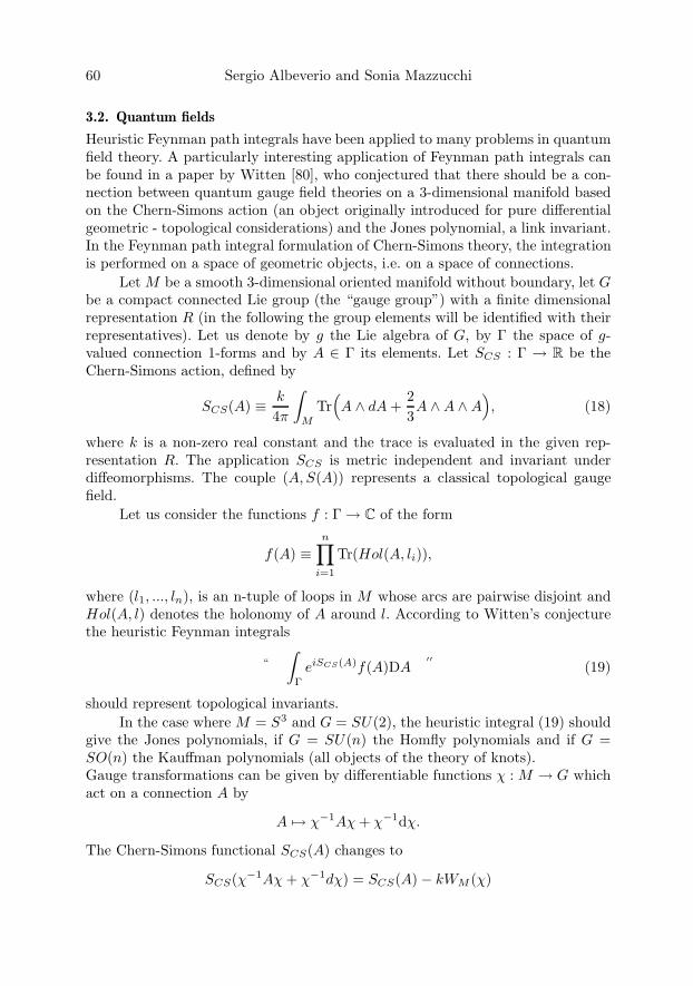
60 Sergio Albeverio and Sonia Mazzucchi
3.2. Quantum fields
Heuristic Feynman path integrals have been applied to many problems in quantumfield theory. A particularly interesting application of Feynman path integrals canbe found in a paper by Witten [80], who conjectured that there should be a con-nection between quantum gauge field theories on a 3-dimensional manifold basedon the Chern-Simons action (an object originally introduced for pure differentialgeometric - topological considerations) and the Jones polynomial, a link invariant.In the Feynman path integral formulation of Chern-Simons theory, the integrationis performed on a space of geometric objects, i.e. on a space of connections.
Let M be a smooth 3-dimensional oriented manifold without boundary, let Gbe a compact connected Lie group (the “gauge group”) with a finite dimensionalrepresentation R (in the following the group elements will be identified with theirrepresentatives). Let us denote by g the Lie algebra of G, by Γ the space of g-valued connection 1-forms and by A ∈ Γ its elements. Let SCS : Γ → R be theChern-Simons action, defined by
SCS(A) ≡ k
4π
∫M
Tr(A ∧ dA +
23A ∧A ∧A
), (18)
where k is a non-zero real constant and the trace is evaluated in the given rep-resentation R. The application SCS is metric independent and invariant underdiffeomorphisms. The couple (A,S(A)) represents a classical topological gaugefield.
Let us consider the functions f : Γ → C of the form
f(A) ≡n∏
i=1
Tr(Hol(A, li)),
where (l1, ..., ln), is an n-tuple of loops in M whose arcs are pairwise disjoint andHol(A, l) denotes the holonomy of A around l. According to Witten’s conjecturethe heuristic Feynman integrals
“
∫Γ
eiSCS(A)f(A)DA′′
(19)
should represent topological invariants.In the case where M = S3 and G = SU(2), the heuristic integral (19) should
give the Jones polynomials, if G = SU(n) the Homfly polynomials and if G =SO(n) the Kauffman polynomials (all objects of the theory of knots).Gauge transformations can be given by differentiable functions χ : M → G whichact on a connection A by
A �→ χ−1Aχ + χ−1dχ.
The Chern-Simons functional SCS(A) changes to
SCS(χ−1Aχ + χ−1dχ) = SCS(A)− kWM (χ)

A Survey of Feynman Path Integrals 61
withWM (χ) ≡ 1
12π
∫M
Tr(χ−1dχ ∧ χ−1dχ ∧ χ−1dχ).
It can be shown that the function eiS : Γ → C is gauge invariant if and only if thequantization condition
kWM (χ) ⊆ 2πZ ∀χ (20)is satisfied (see, e.g., [70]). For abelian G the quantity WM (χ) vanishes, but for ageneral semisimple Lie group G this quantity does not vanish and the quantizationcondition of the coupling constant (20) has to be required [70].
A partial mathematical realization of Witten’s theory was provided in thecase M = R3 by Frohlich and King [39]. Rigorous “algebraic” results, withouthowever any direct relation to Witten’s heuristic path integral approach, can befound in [71].
In the framework of the theory of infinite dimensional oscillatory integrals,the rigorous mathematical realization of the integral (19)
“
∫Γ
eiSCS(A)f(A)DA′′
= IΦ(f)
can be implemented by exploiting suitable gauges, at least under some restrictionon (M,G).
If M is a general manifold with H1(M) = 0 and G is abelian, the integralIΦ(f) has been constructed both as an infinite dimensional oscillatory integral [23]and as a white noise functional [64]. In this case, the integral IΦ(f) represents theGauss linking number of knots. The case where H1(M) �= 0 has been studied byAdams [1] by simplicial methods (related to those first pointed out in [23] on thebasis of [25].
For manifolds M = R3 or M = Σ×R, (Σ being a compact manifold) and Gnon abelian, the construction of the Feynman functional can be implemented inthe framework of the white noise calculus, by exploiting a particular gauge trans-formation (axial gauge) [24]. In this gauge the Chern-Simons action SCS loses thecubic term and the phase function Φ in the integral becomes a quadratic form. Theconstruction of the observables, that is the integrals (19), is rather technical andhas been implemented in [47]. Analogous results have been obtained in the casewhere M = S1 × S2 or M = S1 ×Σ, where Σ is an oriented surface, and G is notabelian by exploiting the “Blau-Thompson’s quasi axial gauge”, also called “torusgauge”[48, 49, 34]. These computations have been performed for “general coloredlinks”. First partial results on the asymptotics in k → ∞ by a rigorous infinitedimensional stationary phase method applied to a regularized Chern-Simons func-tional expressed in terms of Wiener integrals are in [22], where connections withVassiliev’s invariants are mentioned (these invariants appear in a heuristic asymp-totic expansion of the Chern-Simons oscillatory integrals). Much remains obviouslyto do, but it seems that lucky combination of geometrical-algebraic ideas and rigor-ous infinite dimensional analysis related to oscillatory integrals (and probabilisticintegrals) might lead to further exiting developments.

62 Sergio Albeverio and Sonia Mazzucchi
Acknowledgements
The first author is very grateful to the organizers of a most stimulating workshop,with much of the productive interaction between mathematics and physics whichis needed for progress in its fascinating area.
References
[1] R.M. Adams, R-torsion and linking number for simplicial abelian gauge theories.hep-th/9612009 1996
[2] D.H. Adams, S. Sen, Partition function of a quadratic functional and semiclassicalapproximation for Witten’s 3-manifold invariants hep-th/9503095 1995
[3] S. Albeverio. Wiener and Feynman Path Integrals and Their Applications. Proceed-ings of the Norbert Wiener Centenary Congress, 163-194, Proceedings of Symposiain Applied Mathematics 52, Amer. Math. Soc., Providence, RI, 1997.
[4] S. Albeverio, Ph. Blanchard, Ph. Combe, R. Høegh-Krohn, M. Sirugue, Local rel-ativistic invariant flows for quantum fields. Comm. Math. Phys. 90 (3), 329–351(1983).
[5] S. Albeverio, Ph. Blanchard, R. Høegh-Krohn, Feynman path integrals and the traceformula for the Schrodinger operators, Comm. Math. Phys. 83 n.1, 49–76 (1982).
[6] S. Albeverio, A.M. Boutet de Monvel-Berthier, Z. Brzezniak, The trace formula forSchrodinger operators from infinite dimensional oscillatory integrals, Math. Nachr.182, 21–65 (1996).
[7] S. Albeverio and Z. Brzezniak. Finite-dimensional approximation approach to oscil-latory integrals and stationary phase in infinite dimensions. J. Funct. Anal., 113(1):177-244, 1993.
[8] S. Albeverio, Z. Brzezniak, Z. Haba. On the Schrodinger equation with potentialswhich are Laplace transform of measures. Potential Anal. 9 n.1, 65-82, 1998.
[9] S. Albeverio, L. Cattaneo, L. Di Persio, S. Mazzucchi, An infinite dimensional os-cillatory integral approach to the Feynman-Vernon influence functional I, J. Math.Phys. 48, 10, 102109 (2007)
[10] S. Albeverio, G. Guatteri, S. Mazzucchi, Representation of the Belavkin equationvia Feynman path integrals, Probab. Theory Relat. Fields 125, 365–380 (2003).
[11] S. Albeverio, A. Hahn, A. Sengupta, Rigorous Feynman path integrals, with applica-tions to quantum theory, gauge fields, and topological invariants, Stochastic analysisand mathematical physics (SAMP/ANESTOC 2002), 1–60, World Sci. Publishing,River Edge, NJ, (2004).
[12] S. Albeverio and R. Høegh-Krohn. Mathematical theory of Feynman path integrals.2nd edn with S. Mazzucchi, Springer-Verlag, Berlin, 1976 and 2008. Lecture Notesin Mathematics, Vol. 523.
[13] S. Albeverio and R. Høegh-Krohn. Oscillatory integrals and the method of station-ary phase in infinitely many dimensions, with applications to the classical limit ofquantum mechanics. Invent. Math. 40(1), 59-106, 1977.
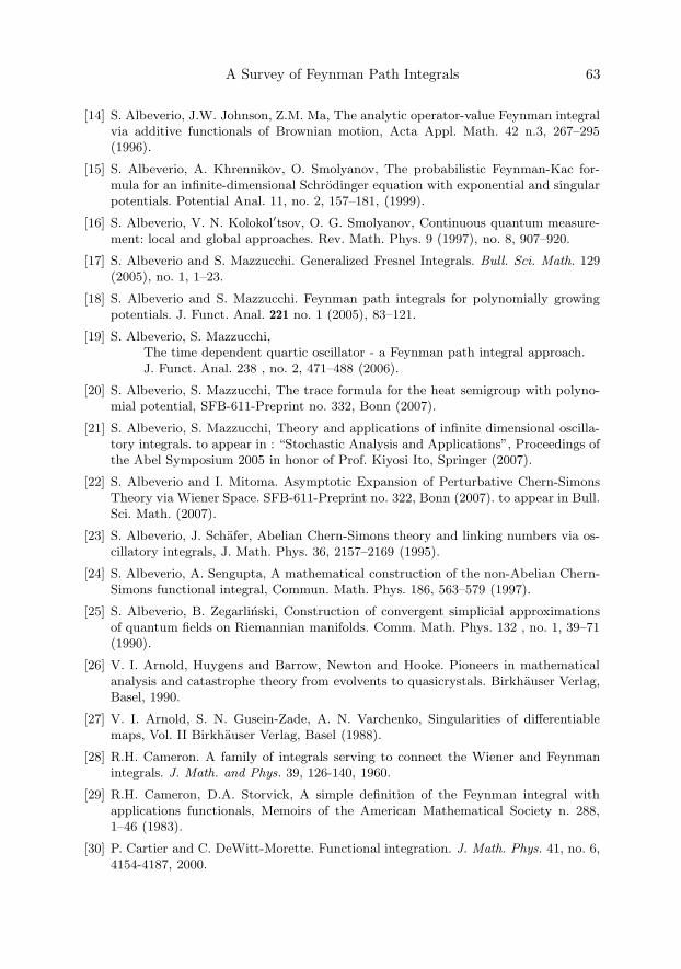
A Survey of Feynman Path Integrals 63
[14] S. Albeverio, J.W. Johnson, Z.M. Ma, The analytic operator-value Feynman integralvia additive functionals of Brownian motion, Acta Appl. Math. 42 n.3, 267–295(1996).
[15] S. Albeverio, A. Khrennikov, O. Smolyanov, The probabilistic Feynman-Kac for-mula for an infinite-dimensional Schrodinger equation with exponential and singularpotentials. Potential Anal. 11, no. 2, 157–181, (1999).
[16] S. Albeverio, V. N. Kolokol′tsov, O. G. Smolyanov, Continuous quantum measure-ment: local and global approaches. Rev. Math. Phys. 9 (1997), no. 8, 907–920.
[17] S. Albeverio and S. Mazzucchi. Generalized Fresnel Integrals. Bull. Sci. Math. 129(2005), no. 1, 1–23.
[18] S. Albeverio and S. Mazzucchi. Feynman path integrals for polynomially growingpotentials. J. Funct. Anal. 221 no. 1 (2005), 83–121.
[19] S. Albeverio, S. Mazzucchi,The time dependent quartic oscillator - a Feynman path integral approach.J. Funct. Anal. 238 , no. 2, 471–488 (2006).
[20] S. Albeverio, S. Mazzucchi, The trace formula for the heat semigroup with polyno-mial potential, SFB-611-Preprint no. 332, Bonn (2007).
[21] S. Albeverio, S. Mazzucchi, Theory and applications of infinite dimensional oscilla-tory integrals. to appear in : “Stochastic Analysis and Applications”, Proceedings ofthe Abel Symposium 2005 in honor of Prof. Kiyosi Ito, Springer (2007).
[22] S. Albeverio and I. Mitoma. Asymptotic Expansion of Perturbative Chern-SimonsTheory via Wiener Space. SFB-611-Preprint no. 322, Bonn (2007). to appear in Bull.Sci. Math. (2007).
[23] S. Albeverio, J. Schafer, Abelian Chern-Simons theory and linking numbers via os-cillatory integrals, J. Math. Phys. 36, 2157–2169 (1995).
[24] S. Albeverio, A. Sengupta, A mathematical construction of the non-Abelian Chern-Simons functional integral, Commun. Math. Phys. 186, 563–579 (1997).
[25] S. Albeverio, B. Zegarlinski, Construction of convergent simplicial approximationsof quantum fields on Riemannian manifolds. Comm. Math. Phys. 132 , no. 1, 39–71(1990).
[26] V. I. Arnold, Huygens and Barrow, Newton and Hooke. Pioneers in mathematicalanalysis and catastrophe theory from evolvents to quasicrystals. Birkhauser Verlag,Basel, 1990.
[27] V. I. Arnold, S. N. Gusein-Zade, A. N. Varchenko, Singularities of differentiablemaps, Vol. II Birkhauser Verlag, Basel (1988).
[28] R.H. Cameron. A family of integrals serving to connect the Wiener and Feynmanintegrals. J. Math. and Phys. 39, 126-140, 1960.
[29] R.H. Cameron, D.A. Storvick, A simple definition of the Feynman integral withapplications functionals, Memoirs of the American Mathematical Society n. 288,1–46 (1983).
[30] P. Cartier and C. DeWitt-Morette. Functional integration. J. Math. Phys. 41, no. 6,4154-4187, 2000.

64 Sergio Albeverio and Sonia Mazzucchi
[31] P. Cartier and C. DeWitt-Morette. Functional integration: action and symmetries.Cambridge Monographs on Mathematical Physics. Cambridge University Press,Cambridge, 2006.
[32] I. Daubechies, J.R. Klauder, Quantum-mechanical path integrals with Wiener mea-sure for all polynomial Hamiltonians. Phys. Rev. Lett. 52 (1984), no. 14, 1161–1164.
[33] I. Daubechies, J.R. Klauder, Quantum-mechanical path integrals with Wiener mea-sure for all polynomial Hamiltonians. II. J. Math. Phys. 26 (1985), no. 9, 2239–2256.
[34] S. de Haro and A. Hahn. The Chern-Simons path integral and the quantum Racahformula. arXiv:math-ph/0611084.
[35] P.A.M. Dirac, The Lagrangian in quantum mechanics, Phys. Zeitschr. d. Sowjetu-nion, 3, No 1, 64–72, 1933.
[36] J.J. Duistermaat. Oscillatory integrals, Lagrange immersions and unfoldings of sin-gularities. Comm. Pure Appl. Math. 27, 207-281, 1974.
[37] D. Elworthy and A. Truman. Feynman maps, Cameron-Martin formulae and anhar-monic oscillators. Ann. Inst. H. Poincare Phys. Theor., 41(2), 115–142, 1984.
[38] R.P. Feynman, A.R. Hibbs. Quantum mechanics and path integrals. Macgraw Hill,New York, 1965.
[39] J. Frohlich, C. King. The Chern-Simons theory and knot polynomials. Comm. Math.Phys. 126, no. 1, 167–199 (1989).
[40] D. Fujiwara, N. Kumano-go, Smooth functional derivatives in Feynman path inte-grals by time slicing approximation,
Bull. Sci. math. 129, 57–79 (2005).
[41] J. Glimm, A. Jaffe, Quantum physics. A functional integral point of view. Secondedition. Springer-Verlag, New York, 1987.
[42] C. Grosche, F. Steiner, Handbook of Feynman path integrals. Springer Tracts inModern Physics, 145. Springer-Verlag, Berlin, 1998.
[43] Z. Haba, Feynman integral and random dynamics in quantum physics. A probabilis-tic approach to quantum dynamics. Mathematics and its Applications, 480. KluwerAcademic Publishers, Dordrecht, 1999.
[44] A. Hahn, Rigorous State Model Representations for the Wilson loop observables inChern-Simons theory, SFB-611-Preprint, Bonn (2002).
[45] A. Hahn, Quasi-Axial Gauge Fixing for Chern-Simons models on S2 ×S1. SFB-611-Preprint, Bonn (2003).
[46] A. Hahn, Chern-Simons theory on R3 in axial gauge: a rigorous approach. J. Funct.Anal. 211 (2004), no. 2, 483–507.
[47] A. Hahn, The Wilson loop observables of Chern-Simons theory on R3 in axial gauge,Commun. Math. Phys. 248 (3), 467–499 (2004).
[48] A. Hahn, Chern-Simons models on S2 × S1, torus gauge fixing, and link invariantsI, J. Geom. Phys. 53 (3), 275–314 (2005).
[49] A. Hahn, An analytic approach to Turaevs shadow invariants, SFB 611 preprint,Bonn, submitted to Commun. Math. Phys.
[50] T. Hida, H.H. Kuo, J. Potthoff, L. Streit, White Noise Kluwer, Dordrecht (1995).
[51] L. Hormander, Fourier integral operators I. Acta Math., 127(1), 79-183, 1971.

A Survey of Feynman Path Integrals 65
[52] L. Hormander. The Analysis of Linear Partial Differential Operators. I. DistributionTheory and Fourier Analysis. Springer-Verlag, Berlin/Heidelberg/New York/Tokyo,1983.
[53] W. Ichinose, A mathematical theory of the phase space Feynman path integral ofthe functional. Comm. Math. Phys. 265 (2006), no. 3, 739–779
[54] T. Ichinose, Path integral for the Dirac equation in two space-time dimensions. Proc.Japan Acad. Ser. A Math. Sci. 58, no. 7, 290–293, (1982).
[55] T. Ichinose, H. Tamura, Propagation of a Dirac particle. A path integral approach.J. Math. Phys. 25, no. 6, 1810–1819 (1984).
[56] K. Ito. Wiener integral and Feynman integral. Proc. Fourth Berkeley Symposium onMathematical Statistics and Probability. Vol 2, pp. 227-238, California Univ. Press,Berkeley, 1961.
[57] K. Ito. Generalized uniform complex measures in the Hilbertian metric space withtheir applications to the Feynman path integral. Proc. Fifth Berkeley Symposium onMathematical Statistics and Probability. Vol 2, part 1, pp. 145-161, California Univ.Press, Berkeley, 1967.
[58] G.W. Johnson, M.L. Lapidus, The Feynman integral and Feynman’s operational cal-culus. Oxford University Press, New York, 2000.
[59] H. Kleinert, Path integrals in quantum mechanics, statistics, polymer physics, andfinancial markets. Third edition. World Scientific Publishing Co., Inc., River Edge,NJ, (2004).
[60] V. N. Kolokoltsov, Complex measures on path space: an introduction to the Feynmanintegral applied to the Schrodinger equation. Methodol. Comput. Appl. Probab. 1(1999), no. 3, 349–365.
[61] V. N. Kolokoltsov, Semiclassical analysis for diffusions and stochastic processes, Lec-ture Notes in Mathematics, 1724. Springer-Verlag, Berlin, (2000).
[62] V. N. Kolokoltsov, A new path integral representation for the solutions of theSchrodinger, heat and stochastic Schrodinger equations. Math. Proc. CambridgePhilos. Soc. 132 (2002), no. 2, 353–375.
[63] T. Kuna, L. Streit, W. Westerkamp, Feynman integrals for a class of exponentiallygrowing potentials, J. Math. Phys. 39, no. 9, 4476–4491 (1998).
[64] S. Leukert, J. Schafer, A Rigorous Construction of Abelian Chern-Simons Path In-tegral Using White Noise Analysis, Reviews in Math. Phys. 8, 445–456 (1996).
[65] P. Malliavin, S. Taniguchi, Analytic functions, Cauchy formula, and stationary phaseon a real abstract Wiener space. J. Funct. Anal. 143 (1997), no. 2, 470–528.
[66] V.P. Maslov. Methodes Operationelles, Mir. Moscou, 1987.
[67] M.B. Mensky, Continuous Quantum Measurements and Path Integrals. Taylor &Francis, Bristol and Philadelphia (1993).
[68] H. J. W. Muller-Kirsten, Introduction to quantum mechanics. Schrodinger equationand path integral. World Scientific Publishing Co. Pte. Ltd., Hackensack, NJ, 2006.
[69] E. Nelson. Feynman integrals and the Schrodinger equation. J. Math. Phys. 5, 332-343, 1964.
[70] M. Niemann, S. Albeverio, A. Hahn, Three remarks on the Chern-Simons quantumfield model, in preparation
66 Sergio Albeverio and Sonia Mazzucchi
[71] N. Reshetkhin, V.G. Turaev, Invariants of 3-manifolds via link polynomials andquantum groups. Invent. Math. 103, no.3, 547–597 (1991).
[72] J. Rezende, The method of stationary phase for oscillatory integrals on Hilbertspaces, Comm. Math. Phys. 101, 187–206 (1985).
[73] G. Roepstorff, Path integral approach to quantum physics. An introduction. Textsand Monographs in Physics. Springer-Verlag, Berlin, (1994).
[74] L. S. Schulman, Techniques and applications of path integration. A Wiley-Interscience Publication. John Wiley & Sons, Inc., New York, 1981.
[75] A. S. Schwartz, The partition function of a degenerate functional. Comm. Math.Phys. 67 , no. 1, 1–16 (1979).
[76] B. Simon, Functional integration and quantum physics. Second edition. AMS ChelseaPublishing, Providence, RI, 2005.
[77] O.G. Smolyanov, A.Yu. Khrennikov, The central limit theorem for generalized mea-sures on infinite-dimensional spaces. (Russian) Dokl. Akad. Nauk SSSR 281 (1985),no. 2, 279–283.
[78] F. Takeo, Generalized vector measures and path integrals for hyperbolic systems.Hokkaido Math. J. 18 (1989), no. 3, 497–511.
[79] H. Thaler. Solution of Schrodinger equations on compact Lie groups via probabilisticmethods. Potential Anal. 18, n.2, 119-140, 2003.
[80] E. Witten, Quantum field theory and the Jones polynomial, Commun. Math. Phys.121, 353–389 (1989).
[81] T. J. Zastawniak, Fresnel type path integral for the stochastic Schrodinger equation.Lett. Math. Phys. 41, no. 1, 93–99 (1997).
Sergio AlbeverioInstitut fur Angewandte MathematikWegelerstr. 6D–53115 BonnandDip. MatematicaUniversita di TrentoI–38050 Povoand BiBoS; IZKS; SFB611; CERFIM (Locarno); Acc. Arch. (Mendrisio)
Sonia MazzucchiInstitut fur Angewandte MathematikWegelerstr. 6D–53115 BonnandDip. MatematicaUniversita di TrentoI–38050 Povo

Quantum Field TheoryB. Fauser, J. Tolksdorf and E. Zeidler, Eds., 67–81c© 2009 Birkhauser Verlag Basel/Switzerland
A Comment on the Infra-Red Problemin the AdS/CFT Correspondence
Hanno Gottschalk and Horst Thaler
Abstract. In this note we report on some recent progress in proving theAdS/CFT correspondence for quantum fields using rigorously defined Eu-clidean path integrals. We also comment on the infra-red problem in theAdS/CFT correspondence and argue that it is different from the usual IRproblem in constructive quantum field theory. To illustrate this, a trivialityproof based on hypercontractivity estimates is given for the case of an ultra-violet regularized potential of type : φ4 :. We also give a brief discussion onpossible renormalization strategies and the specific problems that arise in thiscontext.
Mathematics Subject Classification (2000). Primary 81T08; Secondary 81T30.
Keywords. AdS/CFT correspondence, infra-red problem, constructive quan-tum field theory, triviality results, functional integrals, generating functionals.
1. Introduction
Often, the AdS/CFT correspondence between string theory or some other theoryincluding quantized gravity on bulk AdS and super-symmetric Yang-Mills theoryon its conformal boundary [12, 17] is formulated in terms of Euclidean path in-tegrals. In the absence of mathematically rigorous approaches to path integralsof string type (see however [1]) or even gravity, it seems to be reasonable to usethe well-established theory of constructive quantum field theory (QFT) [5] as atesting lab for some aspects of the more complex original AdS/CFT conjecture.That such simplified versions of the AdS/CFT correspondence are in fact possiblewas already noted by Witten [17] (see also [8]) and further elaborated by [4]. In[6] we give a mathematically rigorous version of the latter work (in [9] one findssome related ideas), leaving however the infra-red (IR) problem open. In this notewe come back to the IR problem and we show how the difference between the IRproblem in the AdS/CFT correspondence as compared with the usual IR problemin constructive QFT leads to somewhat unexpected results.

68 Hanno Gottschalk and Horst Thaler
The authors would like to underline that, in contrast to [6], the present articleis rather focused on ideas and thus leaves space for the interpretation of the validityof the results. We will comment on that in several places.
The article is organized as follows: In the following section we introduce themathematical framework of AdS/CFT correspondence and define rigorous proba-bilistic path integrals on AdS. In Section 3 we recall the main results from [4, 6],i.e. that the generating functional that is obtained from imposing certain boundaryconditions at the conformal boundary (which is the way generating functionals aredefined in string theory) can in fact be written as a usual generating functional ofsome other field theory. From the latter form it is then easy to extract structuralproperties, e.g. reflection positivity of the functional, in the usual way. Somewhatunexpectedly, it is not clear whether a functional integral can be associated tothe boundary theories. These statements hold for all sorts of interactions with aIR-cut-off. In Section 4 the IR-problem in this version of the AdS/CFT corre-spondence is discussed on a heuristic level. We also sketch the proof of trivialityof the generating functional of the conformally invariant theory on the conformalboundary of AdS for the case of an UV-regularized : φ4 : interaction. We brieflysurvey strategies that might be candidates to overcome the triviality obstacle at anon-rigorous level and we comment on specific problems with such strategies. Thefinal section gives some preliminary conclusions and an outlook on open researchproblems in understanding further the mathematical basis of AdS/CFT.
2. Functional integrals on AdS
Let us consider the d+2 dimensional ambient space Rd,2 = Rd+2 with inner productof signature (−,+, . . . ,+,−), i.e. ζ2 = −ζ2
1 +ζ22 + · · ·+ζ2
d+1−ζ2d+2 where ζ ∈ Rd,2.
Then the submanifold defined by {ζ ∈ Rd,2 : ζ2 = −1} is a d + 1 dimensionalLorentz manifold with metric induced by the ambient metric. It is called the d+1dimensional Anti de Sitter (AdS) space. Formal Wick rotation ζ1 → iζ1 convertsthe ambient space into the space Rd+1,1 with signature (+, . . . ,+,−). Under Wickrotation, the AdS space is converted to the Hyperbolic space Hd+1 : {ζ ∈ Rd+1 :ζ2 = −1, ζd > 0}, which is a Riemannian submanifold of the ambient d + 2dimensional Minkowski space. We call Hd+1 the Euclidean AdS space.
It has been established with full mathematical rigor that Euclidean randomfields that fulfil the axioms of invariance, ergodicity and reflection positivity giverise, via an Osterwalder–Schrader reconstruction theorem, to local quantum fieldtheories on the universal covering of the relativistic AdS, cf. [3, 10] justifyingthe above sketched formal Wick rotation. Hence a constructive approach withreflection positive Euclidean functional integrals is viable.
It is convenient to work in the so called half-space model of Euclidean AdS(henceforth the word Euclidean will be dropped). This coordinate system is ob-tained via the change of variables ζi = xi/z, i = 1, . . . , d, ζd+1 = −(z2+x2−1)/2z,ζd+2 = (z2 + x2 + 1)/2z which maps Rd+1
+ = {(z, x) ∈ Rd+1 : z > 0} to Hd+1.

Infra-Red Problem in AdS/CFT 69
We will use the notation x for (z, x1, . . . , xd) ∈ Rd+1+ . The metric on Rd+1
+ is givenby g = (dz2 + dx2
1 + · · · + dx2d)/z2 which implies that the canonical volume form
is dgx = z−d−1dz ∧ dx1 ∧ · · · ∧ dxd. The conformal boundary of Hd+1 then is thed-dimensional Euclidean space Rd with metric ds2 = dx2
1 + · · · + dx2d which is
obtained via the limit z → 0 and a conformal transformation of the AdS metric.Of course, the upshot of the AdS/CFT correspondence is that the action of theLorentz group on the AdS space Hd+1 gives rise to an action of the conformal grouptransformations on the conformal boundary. One thus expects an AdS symmetricQFT (or string/quantum gravity. . . theory) on the bulk Hd+1 to give, if properlyrestricted to the conformal boundary, a conformally invariant theory on Rd.
We will now make this precise. On the hyperbolic space Hd+1 one has twoinvariant Green’s functions (“bulk-to-bulk propagators”) for the operator −Δg +m2, with Δg the Laplacian and m2 a real number suitably bounded from below,that differ by scaling properties towards the conformal boundary
G±(z, x; z′, x′) = γ±(2u)−Δ±F (Δ±,Δ± + 1−d2 ; 2Δ± + 1− d;−2u−1) (2.1)
Here F is the hypergeometric function, u = (z−z′)2+(x−x′)2
2zz′ , Δ± = d2± 1
2
√d2 + 4m2
=: d2 ± ν, ν > 0 and γ± = Γ(Δ±)
2πd/2Γ(Δ±+1− d2 )
[4, 6]. Taking pointwise scaling limitsfor z → 0 in one or two of the arguments, the bulk-to-boundary and boundary-to-boundary propagators are obtained
H±(z, x;x′) = limz′→0
z′−Δ±G±(z, x; z′, x′) = γ±
(z
z2 + (x− x′)2
)Δ±
(2.2)
and
α±(x, x′) = limz→0
z−Δ±H±(z, x;x′) = γ±(x − x′)−2Δ± . (2.3)
If (2.2) or (2.3) do not define locally integrable functions, the expressions on theright hand side are defined via analytic continuation in the weights Δ±. An im-portant relation between G+, G−, H+ and α− is the covariance splitting formulafor G− given by
G−(x, x′) = G+(x, x′) +∫
Rd
∫Rd
H+(x, y)c2α−(y, y′)H+(x′, y′)dydy′, (2.4)
with c = 2ν.We now pass on to the description of mathematically well-defined functional
integrals. Let D = D(Hd+1,R) be the infinitely differentiable, compactly sup-ported functions on Hd+1 endowed with the topology of compact convergence.The propagator G+ is the resolvent function to the Laplacian Δg with Dirichletboundary conditions at conformal infinity, from which it follows that G+ is stochas-tically positive, 〈f, f〉−1 = G+(f , f) =
∫Hd+1×Hd+1 G+(x, x′)f(x)f(x′) dgxdgx
′ ≥ 0
∀f ∈ D, and reflection positive as long as m2 > − d2
4 . The latter value is de-termined by the lower bound of the spectrum of Δg on Hd+1. In explicit, if
70 Hanno Gottschalk and Horst Thaler
θ : (z, x1, x2, . . . , xd) → (z,−x1, x2, . . . , xd) is the reflection in x1-direction, thenfor any f ∈ D+ = {h ∈ D : h(x) = 0 if x1 ≤ 0} we have∫
Hd+1×Hd+1G+(x, x′)fθ(x)f(x′) dgxdgx
′ ≥ 0,
cf. [5]. Here, fu(x) = f(u−1x) for u ∈ Iso(Hd+1).Consequently, via application of Minlos theorem, there exists a unique prob-
ability measure μG+ on the measurable space (D′,B), where D′ is the topo-logical dual space of D and B the associated Borel sigma algebra, such that∫D′ e
〈φ,f〉dμG+(φ) = e12 〈f,f〉−1 . By setting ϕ(f)(φ) = φ(f) we define the canon-
ical random field associated with μG+ , i.e. a random variable valued distribution.In the following we omit the distinction between ϕ and φ and write φ for both.
Let BΛ, Λ ⊆ Hd+1 be the smallest sigma algebra generated by the functionsD′ φ → 〈φ, f〉, suppf ∈ Λ and M(Λ) be the functions that are BΛ-measurable.We use the special abbreviations B+ = B{x∈Hd+1:x1>0} and M+ = M(B+). ThenμG+ is reflection positive, i.e.∫
D′ΘF (φ)F (φ) dμG+(φ) ≥ 0, ∀F ∈M+. (2.5)
The reflection ΘF (φ) is defined as F (φθ) with 〈φu, f〉 = 〈φ, fu−1〉 ∀φ ∈ D′, f ∈D and u ∈ Iso(Hd+1). 〈 . , . 〉 is the duality between D′ and D induced by theL2(Hd+1, dgx) inner product.
Let {VΛ} : D′ → R be a set of interaction potentials indexed by the net ofbounded, measurable subsets Λ in Hd+1. In particular these sets have finite volume|Λ| =
∫Λdgx. We require that the following conditions hold:
(i) Integrability: e−VΛ ∈ L1(D′, dμG+) ∀Λ;(ii) Locality: VΛ ∈M(BΛ);(iii) Invariance: VΛ(φu) = Vu−1Λ(φ) μG+–a.s..(iv) Additivity: VΛ + VΛ′ = VΛ∪Λ′ for Λ ∩ Λ′ = ∅.(v) Non-degeneracy: VΛ = 0 μG+–a.s. if |Λ| = 0.
Then, using (i), we obtain a family of interacting measures on (D′,B), indexedby the net {Λ}, by setting dμG+,Λ = e−VΛdμG+/ZΛ with ZΛ =
∫D′ e
−VΛ dμG+ .Furthermore, using (ii)–(v) we get whenever θΛ = Λ∫
D′ΘFF dμG+,Λ =
1ZΛ
∫D′
Θ(F e−VΛ+
)(Fe−VΛ+
)dμG+ ≥ 0, ∀F ∈M+, (2.6)
where Λ+ = Λ ∩ {x ∈ Hd+1 : x1 > 0}. Hence reflection positivity is preservedunder the perturbation. Furthermore, from the invariance of μG+ under Iso(Hd+1)we get that u∗μG+,Λ = μG+,uΛ. Here u ∈ Iso(Hd+1) induces an action on D′ viaφ → φu and u∗ is the pushforward under this action. Consequently, if the limit(in distribution) μG+,Hd+1 = limΛ↗Hd+1 μG+,Λ exists and is unique, the limitingmeasure is invariant under Iso(Hd+1) and reflection positive. Invariance followsfrom the equivalence of the nets {Λ} and {uΛ} and the postulated uniqueness ofthe limit over the net {Λ}.
Infra-Red Problem in AdS/CFT 71
Let us next consider functional integrals associated with the Green’s functionG−. In the case when 2ν < d (⇔ m2 < 0) we get that α− is stochastically positivesince α−(f , f) =
∫Rd×Rd α−(x, x′)f(x)f(x′) dxdx′ = C−ν
∫Rd |k|−2ν |f(k)|2 dk ≥ 0.
f denotes the Fourier transform of f wrt. x, f(k) = (2π)−d/2∫
Rd eik·xf(x) dx. Fur-
thermore, α− is reflection positive in x1-direction (in the usual sense, cf. [5]) if andonly if −ν > −1, which is also known as the unitarity bound. It is clear from the de-composition (2.4) that G− is stochastically positive if G+ and α− are both stochas-tically positive. The reflection positivity of G− does not follow from the reflectionpositivity of G+ and α− due to the non-local effect of H+. We will however not needit here. We thus conclude that for sup spec(Δg) < m2 < 0 a unique probabilitymeasure μG− on (D′,B) with Laplace transform
∫D′ e
〈φ,f〉dμG−(φ) = e12 〈f,f〉−1,−
exists. Here 〈f, f〉−1,− = G−(f, f). The perturbation of μG− with an interactioncan now be discussed in analogy with the above case – where however the reflec-tion positivity for the perturbed measure remains open, as reflection positivity ofthe free measure does not necessarily hold.
3. Two generating functionals
On the string theory side of the AdS/CFTcorrespondence, generating functionalsfor the boundary theory are calculated fixing boundary conditions at the confor-mal boundary (so called Dirichlet boundary conditions). Little is known about themathematical properties of such kinds of generating functionals. E.g. their sto-chastic and reflection positivity is far from obvious, leaving the linkage to pathintegrals and relativistic physics open. It was noticed by Dutsch and Rehren [4]that such kinds of generating functionals can however be re-written in terms ofordinary generating functionals, from which the structural properties can be readof in the usual way. These ideas in [6] have been made fully rigorous in the contextof constructive QFT. We will now briefly review these results.
The generating functional Z(f)/Z(0), f ∈ S(Rd,R), the space of Schwartzfunctions, in the AdS/CFT correspondence from a string theoretic point of viewcan be described as follows: Let φ be some scalar quantum field that is includedin the theory (e.g. the dilaton field) and let VΛ be the (IR and eventually UV-regularized) effective potential for that field obtained via integrating out the re-maining degrees of freedom (leaving open the question how such an “integral”can be defined). To simplify the model and for the sake of concreteness we willsometimes assume that VΛ is of polynomial type. Formally,
Z(f) =∫
φ0=φ|∂Hd+1=f
e−S0(φ)−VΛ(φ) dφ =∫
δ(φ0 − f)e−S0(φ)−VΛ(φ) dφ (3.1)
where S0 = |∇φ|2 + m2φ2, φ0 = φ|∂Hd+1 are suitably rescaled boundary valuesof the field φ and dφ is the heuristic flat measure on the space of all field con-figurations. The first step in making this formal expression rigorous is to replace
72 Hanno Gottschalk and Horst Thaler
e−S0(φ) dφ with a well-defined probabilistic path integral. It turns out that dμG−(φ)is the right candidate and hence for the moment restriction to m2 < 0 is necessary.
In a second step we have to make sense out of the boundary conditionφ0 = f or the functional delta distribution on the boundary values of the field,respectively. Using the covariance splitting formula (2.4) we obtain the splittingφ−(x) = φ+(x) +
∫Rd H+(x, x′)φα−(x′) dx′, where φ± are the canonical random
fields associated with G± and φα− is the canonical random field associated tothe functional measure μα− , i.e. the Gaussian measure with generating functionale
12 α−(f,f) living on the conformal boundary of Hd+1.
The following step is to construct a finite dimensional approximation ψα− ofthe boundary field φα− by projecting it via a basis expansion to Rn. Thereafter,one can implement the delta distribution as a delta distribution on Rn. Finallyone can remove the finite dimensional approximation via a limit n→∞. It turnsout that this limit exists and is unique up to a diverging multiplicative constant.This constant however drops out in the quotient Z(f)/Z(0). With the projectionto the first n terms of the basis expansion denoted by pn and η a linear mappingfrom this space to Rn we get
CA−
∫Rn
∫D′
δ(ψα− − ηpnf)e−VΛ(φ++cH+(η−1ψα− ))dμG+(φ+)e−12 (ψα− ,A−ψα− )dψα−
= CA−e− 1
2 (f,(pnα−pn)−1f)
∫D′
e−VΛ(φ++cH+(pnf))dμG+(φ+) =: Zn(f), (3.2)
where A− := (ηpnα−pnη−1)−1 and CA− = |detA−| 12
(2π)d2
. One can then show that
Z(f)/Z(0) := limn→∞Zn(f)/Zn(0) = e−
12 (f,α−1
− f)
∫D′ e
−VΛ(φ++cH+f)dμG+(φ+)∫D′ e−VΛ(φ+)dμG+(φ+)
(3.3)converges under rather weak continuity requirements on VΛ that are fulfilled e.g. forUV-regularized potentials in arbitrary dimension and for P (φ)2 potentials withoutUV cut-offs in d+1 = 2. Obviously, the limit does not depend on the details of thefinite dimensional approximation. For the details we refer to [6]. We now realizethat the right hand side of (3.3) also makes sense for m2 ≥ 0 and we adopt (3.3)as a definition of (3.1).
At this point one would like to associate a boundary field theory to thegenerating functional C(f) = Z(f)/Z(0). In order to obtain a functional in-tegral associated to C : S = S(Rd,R) → R we require that C is continuouswrt. the Schwartz topology, normalized, C(0) = 1 and stochastically positive,∑n
j,l=1 zjzlC(fj + fl) ≥ 0 ∀ n ∈ N, fj ∈ S, zj ∈ C. Furthermore, in order tohave a well defined passage from Euclidean time to real time QFT one requiresreflection positivity
∑nj,l=1 zjzlC(fj,θ + fl) ≥ 0 ∀ n ∈ N, fj ∈ S+, zj ∈ C. Here
S+ = {f ∈ S : suppf ⊆ {x ∈ Rd : x1 > 0}}. Finally, the theory obtained at theboundary should be conformally invariant, provided the IR cut-off Λ is removedfrom VΛ via taking the limit of the generating functionals wrt. the net {Λ}.

Infra-Red Problem in AdS/CFT 73
It has been pointed out in [4, 11, 16] that an alternative representation of thefunctional (3.3) answers a number of the questions raised above. Let φ(x) = φ(z, x)be the canonical random field associated with the measure μG+ . The idea is tosmear φ(z, x) in the x-variable with a test function f ∈ D(Rd,R) and then scalez → 0. In the light of (2.1), one has to multiply φ(z, f) = 〈φ, δz ⊗ f〉 with a factorz−Δ+ in order to obtain a finite result in the limit. We set
Yz(f) =∫D′
e〈φ,z−Δ+δz⊗f〉e−VΛ(φ) dμG+(φ). (3.4)
Clearly, under the conditions on VΛ given in the preceding section and for Λ = θΛ,Yz(f)/Yz(0) defines a continuous, normalized, stochastically positive and reflectionpositive generating functional for all z > 0. Using the fact that G+(δz ⊗ f) is inthe Cameron-Martin space of the measure μG+ , one gets with fz = z−Δ+δz ⊗ f ,cf. [6],
Yz(f)/Yz(0) = e12 G+(fz,fz)
∫D′
e−VΛ(φ+G+fz)dμG+(φ)/Yz(0). (3.5)
We now want to take the limit z → 0. Using (2.2) one can show under ratherweak continuity requirements on VΛ that the functional integral on the rhs of (3.5)converges to
∫D′ e
−VΛ(φ+H+f)dμG+(φ). The prefactor however diverges. The reasonis that the limit in (2.3) is only a pointwise limit for x �= x′ and not a limit in thesense of tempered distributions. One can however show that [6]∫
Rd
∫Rd
α+(x, y)f(x)f(y)dxdy =
limz→0
z−2Δ+
∫Rd
∫Rd
G+(z, x; z, y)f(x)f(y)dxdy−
1
(2π)d2
(21−ν
√πΓ(ν + 1
2 )
)2 [ν]∑j=0
z−2(ν−j)(−1)jaj
∫Rd
|f(k)|2|k|2jdk.
=: limz→0
z−2Δ+
∫Rd
∫Rd
G+(z, x; z, y)f(x)f(y)dxdy − (Corr(z)f, f). (3.6)
Here aj =∫∞0
(∫ 1
0cos(ωt)(1− t2)ν− 1
2 dt)2ω2(ν−j)−1dω. Thus, the right hand side of(3.5) multiplied with e−
12 (Corr(z)f,f) converges and we obtain the limiting functional
C(f) = limz→0
e−12 (Corr(z)f,f) (Yz(f)/Yz(0))
= limz→0
e12 [G+(fz,fz)−(Corr(z)f,f)]
∫D′
e−VΛ(φ+G+fz)dμG+(φ)/Yz(0)
= e12 α+(f,f)
∫D′ e
−VΛ(φ+H+f)dμG+(φ)∫D′ e−VΛ(φ)dμG+(φ)
(3.7)
This, together with α−1− = −c2α+, establishes the crucial identity [4, 6]
C(f) = C(cf), ∀f ∈ S(Rd,R). (3.8)

74 Hanno Gottschalk and Horst Thaler
Let us now investigate the structural properties of the generating functional C :S → R. If there were not the correction factor (Corr(z)f, f), C would be stochas-tically positive and reflection positive as the limit of functionals with that prop-erty, since we can combine (3.7) and (3.8) for a representation of C. However,due to the signs in (3.6) S f → e−
12 (Corr(z)f,f) ∈ R is not stochastically posi-
tive and consequently the stochastic positivity of e−12 (Corr(z)f,f) (Yz(f)/Yz(0)) is
at least unclear. Hence we do not have any reason to believe that the limitingfunctional C is stochastically positive and can be associated with a probabilisticfunctional integral. An exception is the case where VΛ ≡ 0 where we can dwellon the fact that S f → e
12 α+(f,f) ∈ R is manifestly stochastically positive since
α(k) = C−ν
(|k|2
)2ν
∈ R with C−ν > 0. It is therefore questionable if one canuse the AdS/CFT correspondence to generate conformally invariant models instatistical mechanics.
We next investigate the question of reflection positivity. Since the correlationlength of the distributional kernels of Corr(z) is zero, we get that (Corr(z)(fj,θ +fl), (fj,θ + fl)) = (Corr(z)fj,θ, fj,θ) + (Corr(z)fl, fl) = (Corr(z)fj , fj) +(Corr(z)fl, fl) for fj ∈ S+. Consequently, ∀fj ∈ S+, z1, . . . , zn ∈ C and Λ suchthat θΛ = Λ we get
n∑j,l=1
C(fj,θ + fl)zjzl = limz→0
n∑j,l=1
(Yz(cfj,θ + cfl)/Yz(0)) z′jz′l ≥ 0 (3.9)
with z′j = zje− 1
2 (Corr(z)cfj ,cfj). For a proof that the reflection positivity of gener-ating functionals implies the reflection positivity of Schwinger functions [5] alsoin the absence of stochastic positivity, cf. [7]. As in [4, 6, 16], we thus come tothe conclusion that the crucial property for the existence of a relativistic theory ispreserved in the AdS/CFT correspondence.
Finally we address the invariance properties of the limiting generating func-tional C. For being the generating functional of a CFT, we require invariance underconformal transformations, i.e. C(f) = C(λ−1
u fu) ∀f ∈ S where u is an element ofthe conformal group on Rd and
λu(x) =∣∣∣∣det
(∂u(x)∂x
)∣∣∣∣−Δ+
d
. (3.10)
Certainly, as long as an interaction with IR cut-off is included in the definition ofC = CΛ, conformal invariance can not hold. Using the identification of Iso(Hd+1)and the conformal group on Rd, we get that H+ intertwines the respective repre-sentations on function spaces, i.e. [6]
H+(u(z, x);x′) =∣∣∣∣det
(∂u−1(x′)
∂x′
)∣∣∣∣Δ+
d
H+(z, x;u−1(x′)). (3.11)
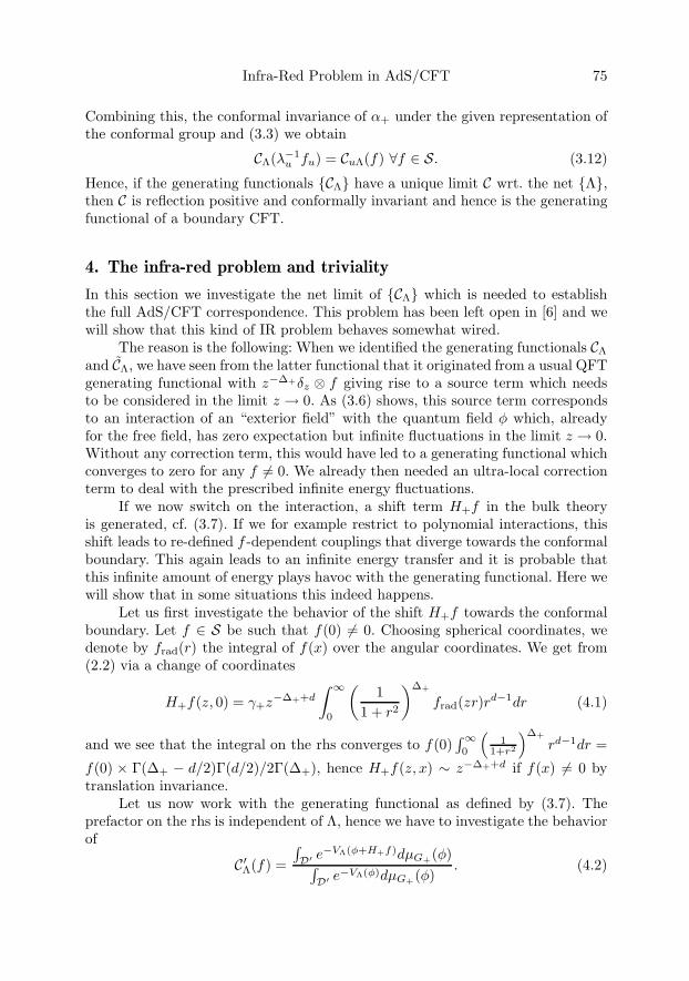
Infra-Red Problem in AdS/CFT 75
Combining this, the conformal invariance of α+ under the given representation ofthe conformal group and (3.3) we obtain
CΛ(λ−1u fu) = CuΛ(f) ∀f ∈ S. (3.12)
Hence, if the generating functionals {CΛ} have a unique limit C wrt. the net {Λ},then C is reflection positive and conformally invariant and hence is the generatingfunctional of a boundary CFT.
4. The infra-red problem and triviality
In this section we investigate the net limit of {CΛ} which is needed to establishthe full AdS/CFT correspondence. This problem has been left open in [6] and wewill show that this kind of IR problem behaves somewhat wired.
The reason is the following: When we identified the generating functionals CΛ
and CΛ, we have seen from the latter functional that it originated from a usual QFTgenerating functional with z−Δ+δz ⊗ f giving rise to a source term which needsto be considered in the limit z → 0. As (3.6) shows, this source term correspondsto an interaction of an “exterior field” with the quantum field φ which, alreadyfor the free field, has zero expectation but infinite fluctuations in the limit z → 0.Without any correction term, this would have led to a generating functional whichconverges to zero for any f �= 0. We already then needed an ultra-local correctionterm to deal with the prescribed infinite energy fluctuations.
If we now switch on the interaction, a shift term H+f in the bulk theoryis generated, cf. (3.7). If we for example restrict to polynomial interactions, thisshift leads to re-defined f -dependent couplings that diverge towards the conformalboundary. This again leads to an infinite energy transfer and it is probable thatthis infinite amount of energy plays havoc with the generating functional. Here wewill show that in some situations this indeed happens.
Let us first investigate the behavior of the shift H+f towards the conformalboundary. Let f ∈ S be such that f(0) �= 0. Choosing spherical coordinates, wedenote by frad(r) the integral of f(x) over the angular coordinates. We get from(2.2) via a change of coordinates
H+f(z, 0) = γ+z−Δ++d
∫ ∞
0
(1
1 + r2
)Δ+
frad(zr)rd−1dr (4.1)
and we see that the integral on the rhs converges to f(0)∫∞0
(1
1+r2
)Δ+
rd−1dr =
f(0) × Γ(Δ+ − d/2)Γ(d/2)/2Γ(Δ+), hence H+f(z, x) ∼ z−Δ++d if f(x) �= 0 bytranslation invariance.
Let us now work with the generating functional as defined by (3.7). Theprefactor on the rhs is independent of Λ, hence we have to investigate the behaviorof
C′Λ(f) =
∫D′ e
−VΛ(φ+H+f)dμG+(φ)∫D′ e−VΛ(φ)dμG+(φ)
. (4.2)

76 Hanno Gottschalk and Horst Thaler
We restrict ourselves to the simplest possible case - an ultra-violet regularized φ4
potential in arbitrary dimensions d + 1
VΛ(φ) = λ
∫Λ
: φ4κ : (x) dgx (4.3)
where φκ denotes the random field φ with UV-cut off κ. Due to this cut-off,the locality axiom in Section 2 will in general be violated. This however doesnot matter in the following discussion. We furthermore require that Gκ
+(x, x′) =E[φκ(x)φκ(x′)] is a bounded function in x and x′. E stands for the expectationwrt. μG+ . The Wick ordering in (4.3) is taken wrt. G+, for simplicity. The shiftedpotential then is given by
VΛ(φ + H+f) = λ
∫Λ
4∑j=0
(4j
): φj
κ : (x)(H+f)4−j(x) dgx. (4.4)
Taking the expected value of the shifted potential wrt. μG+ , one obtains λ××∫Λ(H+f)4dgx which in the light of (4.1) clearly diverges as Λ ↗ Hd+1 whenever
f �= 0.Let us now focus on a specific class of cut-offs of the form Λ(z0) = Λ(z0, l) =
[z0, A] × [−l, l]×d where we keep l > 0, A > 0 arbitrarily large but fixed. LetV (z0, f)(φ) = VΛ(z0)(φ + H+f). Since dgx = z−d−1dzdx we obtain the scaling ofthe expected shifted interaction energy
E(z0, f) = E[V (z0, f)] = λ
∫[z0,A]
∫[−l,l]×d
(H+f)4(z, x) dxz−d−1dz
∼ z−d−4(Δ+−d)0 as z0 → 0. (4.5)
Let us next investigate the fluctuations in the shifted energy as z0 → 0. Denotingthe standard deviation of V (z0, f) with σ(z0, f), we obtain using (4.4) and E[: φa
κ :(x) : φb
κ : (y)] = a! δa,bGκ+(x, y)a, a, b ∈ N,
σ(z0, f) =
[24
∫Λ(z0)×2
Gκ+(x, y)4dgxdgy
+ 96∫Λ(z0)×2
H+f(x)H+f(y)Gκ+(x, y)3dgxdgy
+ 72∫Λ(z0)×2
(H+f)2(x)(H+f)2(y)Gκ+(x, y)2dgxdgy
+ 16∫
Λ(z0)×2(H+f)3(x)(H+f)3(y)Gκ
+(x, y)dgxdgy
]1/2
(4.6)
∼ z−d−3(Δ+−d)0 or slower as z0 → 0,
where we took the factors Gκ+ out of the integral and replaced them with a ma-
jorizing constant in order to obtain an upper bound on the scaling. Apparently, the

Infra-Red Problem in AdS/CFT 77
quotient γ(z0, f) = 2σ(z0, f)/E(z0, f) ∼ zΔ+−d0 scales down to zero if m2 > 0. Us-
ing the Chebychev inequality μG+(|V (z0, f)− E(z0, f)| ≤ E(z0, f)/2) ≤ γ(z0, f)2
we see from this that V (z0, f) →∞ μG+ -a.s..To determine the behavior of C′Λ(z0)
(f) for f �= 0 we however need an argu-ment based on the hypercontractivity estimate ‖F‖p ≤ (p − 1)n/2‖F‖2 ∀F thatare in the Lp(D′,B, μG+)-closure of the span of Wick monomials : φ(f1) · · ·φ(fs) :with s ≤ n. Applying this to V (z0, f) = VΛ(z0)(φ + H+f) with n = 4 one obtains
μG+
(V (z0, f) ≤ E(z0, f)
2
)≤ μG+
(|V (z0, f)− E(z0, f)| ≥ E(z0, f)
2
)≤ 2p
E(z0, f)p‖V (z0, f)− E(z0, f)‖p
p
≤ 2p
E(z0, f)p(p− 1)2p ‖V (z0, f)− E(z0, f)‖p
2
= γ(z0, f)p(p− 1)2p. (4.7)
The next step is to optimize this estimate wrt. p for z0 → 0. Equivalently, onecan ask for the minimum of the logarithm of the rhs wrt. to p. Taking the p-derivative of this expression and setting it zero yields 0 = log γ(z0, f) + 2p(z0)
p(z0)−1 +2 log(p(z0) − 1) with p(z0) the optimal p. Apparently, p(z0) → ∞ as z0 → 0 andthus 2p(z0)/(p(z0)− 1) → 2, hence p(z0) scales as
p(z0) ∼ e−1 × γ(z0, f)−1/2 ∼ Ce−1 × z−(Δ+−d)/20 . (4.8)
Combining (4.7) and (4.8) yields
μG+
(V (z0, f) <
E(z0, f)2
)≤
γ(z0, f)e−1×γ(z0,f)−1/2(e−1 × γ(z0, f)−1/2 − 1
)2e−1×γ(z0,f)−1/2
∼ e−2e−1×γ(z0,f)−1/2
∼ e−2Ce−1×z(d−Δ+)/20 (4.9)
We have thus seen that the portion of the probability space where V (z0, f) doesnot get large as z0 → 0 has a rapidly falling probability. We need an estimatethat controls the negative values on this exceptional set. The ultra-violet cut-offimplies : φ4
κ : (x) ≥ −Bc2κ, B independent of κ, cκ = supx,y |Gκ(x, y)|, μG+ -a.s.,which provides us with a pointwise lower bound for V (z0, f) that is depending onz0 as
V (z0, f) ≥ −λBc2κ|Λ(z0)| = −[λBc2κ(2l)d]× (z−d0 −A−d)/d μG+ − a.s. (4.10)
Combination of (4.9) and (4.10) gives for z0 sufficiently small
E[e−V (z0,f)
]≤ e−
12 E(z0,f)+e[λBc2
κ(2l)d]×(z−d0 −A−d)/d−2Ce−1×z
(d−Δ+)/20 → 0 (4.11)
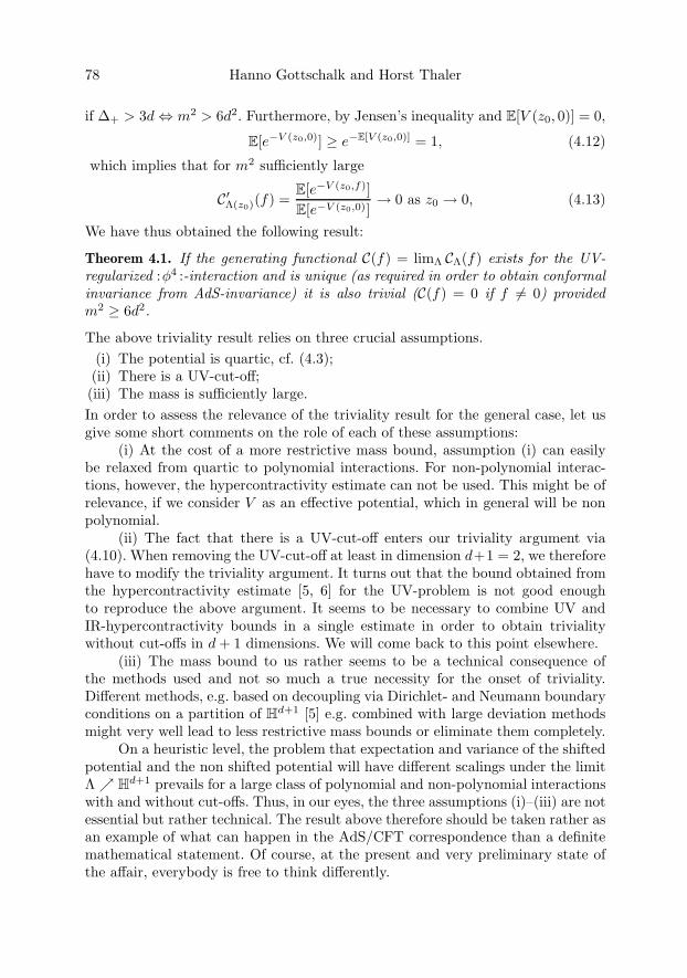
78 Hanno Gottschalk and Horst Thaler
if Δ+ > 3d⇔ m2 > 6d2. Furthermore, by Jensen’s inequality and E[V (z0, 0)] = 0,
E[e−V (z0,0)] ≥ e−E[V (z0,0)] = 1, (4.12)
which implies that for m2 sufficiently large
C′Λ(z0)(f) =
E[e−V (z0,f)]E[e−V (z0,0)]
→ 0 as z0 → 0, (4.13)
We have thus obtained the following result:
Theorem 4.1. If the generating functional C(f) = limΛ CΛ(f) exists for the UV-regularized :φ4 :-interaction and is unique (as required in order to obtain conformalinvariance from AdS-invariance) it is also trivial (C(f) = 0 if f �= 0) providedm2 ≥ 6d2.
The above triviality result relies on three crucial assumptions.(i) The potential is quartic, cf. (4.3);(ii) There is a UV-cut-off;(iii) The mass is sufficiently large.In order to assess the relevance of the triviality result for the general case, let usgive some short comments on the role of each of these assumptions:
(i) At the cost of a more restrictive mass bound, assumption (i) can easilybe relaxed from quartic to polynomial interactions. For non-polynomial interac-tions, however, the hypercontractivity estimate can not be used. This might be ofrelevance, if we consider V as an effective potential, which in general will be nonpolynomial.
(ii) The fact that there is a UV-cut-off enters our triviality argument via(4.10). When removing the UV-cut-off at least in dimension d+1 = 2, we thereforehave to modify the triviality argument. It turns out that the bound obtained fromthe hypercontractivity estimate [5, 6] for the UV-problem is not good enoughto reproduce the above argument. It seems to be necessary to combine UV andIR-hypercontractivity bounds in a single estimate in order to obtain trivialitywithout cut-offs in d + 1 dimensions. We will come back to this point elsewhere.
(iii) The mass bound to us rather seems to be a technical consequence ofthe methods used and not so much a true necessity for the onset of triviality.Different methods, e.g. based on decoupling via Dirichlet- and Neumann boundaryconditions on a partition of Hd+1 [5] e.g. combined with large deviation methodsmight very well lead to less restrictive mass bounds or eliminate them completely.
On a heuristic level, the problem that expectation and variance of the shiftedpotential and the non shifted potential will have different scalings under the limitΛ ↗ Hd+1 prevails for a large class of polynomial and non-polynomial interactionswith and without cut-offs. Thus, in our eyes, the three assumptions (i)–(iii) are notessential but rather technical. The result above therefore should be taken rather asan example of what can happen in the AdS/CFT correspondence than a definitemathematical statement. Of course, at the present and very preliminary state ofthe affair, everybody is free to think differently.

Infra-Red Problem in AdS/CFT 79
5. Conclusions and outlook
In this section we give an essentially non-technical discussion on repair strategiesthat would cure the obstacle of triviality.
(i) coupling constant renormalization: The simplest way to deal with the di-vergences in the potential energy V (z0, f) would be to make λ a z0-dependentquantity. In fact, a naive guess at the scaling behavior suggests that λ(z0) ∼z
d+4(Δ+−d)0 would compensate for the increase in the expected value of the inter-
action energy V (z0, f) such that with the modified coupling limz0→0 E[V (z0, f)] =λC
∫Rd f
4 dx converges to a constant with C = (γ+Γ(Δ+ − d/2)Γ(d/2)/2Γ(Δ+))4,cf. (4.1) and the paragraph thereafter. Furthermore, one can expect that the sub-leading terms (j = 1 . . . 4 in (4.4)) converge to zero and do not affect the generatingfunctional. It thus seems reasonable that with this renormalization the generatingfunctional gives in the limit z0 → 0
C(f) = e12 α+(f,f)−λC
∫Rd f4 dx (5.1)
which is reflection positive as a limit of reflection positive functionals (it is man-ifestly not stochastically positive for all λ > 0 and hence gives a nice illustrationfor the destruction of stochastic positivity due to the correction term in (3.6) and(3.7). The problem with this functional however is that the additional term in theinteraction is an ultra local term and hence does not influence the correspondingreal time CFT – which is a free theory determined by the analytic continuation ofα+. Hence this sort of renormalization only trades in another kind of triviality forthe triviality observed in Section 4.
(ii) bulk counterterms: Such terms can simply be added to the (formal) La-grangian. The problem to use this method in the AdS/CFT correspondence istwofold: Firstly, the infra-red divergences that are occurring in V (z0, f) are f -dependent. If we however want to cure them with f -dependent counterterms,the renormalization description of CΛ(z0) becomes f -dependent. Bulk countert-erms however only preserve the structural properties of stochastic and reflectionpositivity, if the same renormalization prescription is chosen for all f . Hence, f -dependent counterterms would lead to a limiting functional, for which it is notknown, whether it is reflection positive or not. The situation is worsened from theobservation that, unlike in other IR problems, in the AdS/CFT correspondencethe divergences in the nominator and denominator scale differently - as seen in ourtriviality result. This means for bulk counterterms, that, if they are working outfine for the nominator, they probably create new divergences in the denominator.Different renormalizations for the potential in the nominator and in the denomina-tor in the limit might lead to a non normalizable vacuum for the boundary theory,which does not make sense.
(iii) boundary counterterms: The problems described above for bulk coun-terterms also have to be taken into account for boundary counterterms. Further-more, while bulk counterterms, at least if they are not f -dependent, do not spoil
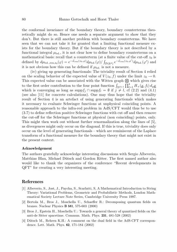
80 Hanno Gottschalk and Horst Thaler
the conformal invariance of the boundary theory, boundary counterterms theo-retically might do so. Hence one needs a separate argument to show that theydon’t. But there is still another problem with boundary counterterms. We haveseen that we can not take it for granted that a limiting functional measure ex-ists for the boundary theory. But if the boundary theory is not described by afunctional integral μbd., it is not clear how to define boundary counterterms on amathematical basis: recall that a counterterm (at a finite value of the cut-off z0 isdefined by dμbd.,ren,z0(ϕ) = e−Lren(z0,ϕ)dμbd.(ϕ)/
∫D(Rd) e
−Lren(z0,ϕ′)dμbd.(ϕ′) andit is not obvious how this can be defined if μbd. is not a measure.
(iv) giving up generating functionals: The triviality result of Section 4 reliedon the scaling behavior of the expected value of V (z0, f) under the limit z0 → 0.This expected value can be associated with the Witten graph
⊗which gives rise
to the first order contribution to the four point function∫
Hd+1
∏4l=1 H+(x, fl) dgx
which is converging as long as suppfj ∩ suppfl = ∅ if j �= l, cf (2.2) and (4.1)(see also [11] for concrete calculations). One may thus hope that the trivialityresult of Section 4 is an artefact of using generating functionals which makesit necessary to evaluate Schwinger functions at unphysical coinciding points. Areasonable approach to the infra-red problem in AdS/CFT would thus be to use(3.7) to define reflection positive Schwinger functions with cut off and then removethe cut-off for the Schwinger functions at physical (non coinciding) points, only.This might then work out without further renormalization along the lines of [5],as divergences might only occur on the diagonal. If this is true, triviality does onlyoccur on the level of generating functionals – which are reminiscent of the Laplacetransform of a functional measure for the boundary theory that might not exist inthe present context.
Acknowledgement
The authors gratefully acknowledge interesting discussions with Sergio Albeverio,Matthias Blau, Michael Dutsch and Gordon Ritter. The first named author alsowould like to thank the organizers of the conference “Recent developments inQFT” for creating a very interesting meeting.
References
[1] Albeverio, S., Jost, J., Paycha, S., Scarlatti, S, A Mathematical Introduction to StringTheory: Variational Problems, Geometric and Probabilistic Methods, London Math-ematical Society Lecture Note Series, Cambridge University Press 1997.
[2] Bertola M., Bros J., Moschella U., Schaeffer R.: Decomposing quantum fields onbranes. Nuclear Physics B 581, 575-603 (2000)
[3] Bros J., Epstein H., Moschella U.: Towards a general theory of quantized fields on theanti-de Sitter spacetime. Commun. Math. Phys. 231, 481-528 (2002)
[4] Dutsch M., Rehren K.H.: A comment on the dual field in the AdS-CFT correspon-dence. Lett. Math. Phys. 62, 171-184 (2002)
Infra-Red Problem in AdS/CFT 81
[5] Glimm J., Jaffe A.: Quantum Physics. A Functional Integral Point of View, 2ndedition. Springer, New-York 1987
[6] Gottschalk, H., Thaler, H.: AdS/CFT correspondence in the Euclidean context, math-ph/0611006, to appear in Commun. Math. Phys.
[7] Gottschalk H.: Die Momente gefalteten Gauß-Poissonschen weißen Rauschens alsSchwingerfunktionen. Diploma thesis, Bochum 1995
[8] Gubser S.S., Klebanov I.R., Polyakov A.M.: Gauge theory correlators from noncriticalstring theory. Phys. Lett. B 428, 105-114 (1998)
[9] Haba Z.: Quantum field theory on manifolds with a boundary. J. Phys. A 38, 10393-10401 (2005)
[10] Jaffee A., Ritter G.: Quantum field theory on curved backgrounds II: Spacetimesymmetries. arXiv:0704.0052v1 [hep-th]
[11] Kniemeyer O.: Untersuchungen am erzeugenden Funktional der AdS-CFT-Korre-spondenz. Diploma thesis, Univ. Gottingen 2002
[12] Maldacena J.: The large N limit of superconformal field theories and supergravity.Adv. Theor. Math. Phys. 2, 231-252 (1998)
[13] Osterwalder K., Schrader R.: Axioms for Euclidean Green’s functions. Comm. Math.Phys. 31, 83-112 (1973)
[14] Osterwalder K., Schrader R.: Axioms for Euclidean Green’s functions. II. With anappendix by Stephen Summers. Comm. Math. Phys. 42, 281–305 (1975)
[15] Rehren K.-H.: Algebraic holography. Ann. Henri Poincare 1, 607-623 (2000)
[16] Rehren, K.-H.: QFT lectures on AdS-CFT, arXiv:hep-th/0411086v1
[17] Witten E.: Anti-de Sitter space and holography. Adv. Theor. Math. Phys. 2, 253-291(1998)
Hanno GottschalkInstitut fur Angewandte MathematikWegelerstr. 6D–53115 Bonne-mail: [email protected]
Horst ThalerDipartimento di Matematica e InformaticaUniversita di CamerinoI–62032 Camerinoe-mail: [email protected]

Quantum Field TheoryB. Fauser, J. Tolksdorf and E. Zeidler, Eds., 83–94c© 2009 Birkhauser Verlag Basel/Switzerland
Some Steps Towards NoncommutativeMirror Symmetry on the Torus
Karl-Georg Schlesinger
Abstract. Starting from motivating examples, we discuss some aspects of thequestion how to extend mirror symmetry to the case of the noncommutativetorus. Following the - by now classical - approach of Dijkgraaf to mirrorsymmetry on elliptic curves, we will see how elliptic deformations of specialfunctions (especially, the elliptic gamma function) arise. In the final sectionwe indicate a possible way how these results might relate to deformations ofFukaya categories of elliptic curves.
Mathematics Subject Classification (2000). Primary 14J32; Secondary 14J15;14J81.
Keywords. mirror symmetry, elliptic curves, noncommutative torus, stringduality, Fukaya category, Gromov-Witten invariants.
1. Introduction
Mirror symmetry is a duality symmetry between certain two dimensional super-conformal field theories which was discovered in the context of string theory inthe early 1990s. Applied to sigma models, this leads to a completely new sym-metry between Calabi-Yau spaces (of, in general, even differing topology). It isan open question if and how this duality might extend to the case of noncommu-tative spaces. There is far reaching work using the language of noncommutativealgebraic geometry (see e.g. [11], [12], [19] and literature cited therein, to give anon-exhaustive selection), dealing with this question. We will follow a much moremodest goal in these notes, restricting completely to the case of noncommutativeelliptic curves (i.e. a noncommutative torus equipped with some additional struc-ture). We still think that an approach focused on only one class of examples isjustified since even in the commutative case the elliptic curve provides a highlynontrivial example for homological mirror symmetry.
84 Karl-Georg Schlesinger
The extension of mirror symmetry to noncommutative spaces is definitelynot an example of generalization for the sake of generalization. We restrict, here,to two motivating examples (for additional motivation, see e.g. [12]).
In [20] the geometric Langlands correspondence is related to mirror symme-try for sigma models with a Hitchin moduli space target, for the special case ofvanishing B-field. If a B-field is turned on in the sigma model, one gets a de-formation to a noncommutative setting (twisted D-modules, quantum geometricLanglands correspondence). More generally, coupling of a B-field to both sides ofthe duality, the A- and the B-model, needs a noncommutative extension of mirrorsymmetry (see [24]).
Another concrete example of this type is provided by the D5-brane gaugetheory in type IIB string theory. Here, the generalization to the noncommutativecase is not just an option but is necessary for the existence of a space-fillingcoisotropic brane (which is decisive for the existence of a D-module structure onA-branes in [20]). We refer to [34] for the details of this example.
These notes are organized as follows: First, we review some needed results forthe classical case of (commutative) elliptic curves. Next, we give our results for thenoncommutative case (for the details we refer, again, to [34]). Especially, we suggesta formal extension of Gromov-Witten invariants to the case of noncommutativeelliptic curves. In the final section, we give some preliminary arguments how ourresults might relate to certain exotic deformations of the Fukaya category of anelliptic curve. This is work in progress.
2. Elliptic curves
Mirror symmetry for elliptic curves was extensively studied in the mid 1990s (seeespecially [8], [9], [10], [16], [31]). It was a prime motivating source for the homo-logical mirror symmetry conjecture of [17]. A proof of homological mirror symme-try for elliptic curves was established in [29]. The Strominger-Yau-Zaslow conjec-ture ([39]), proposing another mathematical formulation of mirror symmetry, wasproved for elliptic curves (and, more generally, for Abelian varieties) in [18].
An elliptic curve Et,τ is a smooth 2-torus equipped with a holomorphic anda symplectic structure. The holomorphic structure - parameterized by τ - is givenby the representation of the elliptic curve as
C/ (Z⊕ Zτ)
with τ = τ1 + iτ2 ∈ C from the upper half plane H, i.e. τ2 > 0. The symplecticstructure - parameterized by t ∈ H - is given by the complexified Kahler class[ω] ∈ H2 (Et,τ ,C) with
ω = −πt
τ2dz ∧ dz
and for t = t1 + it2 the area of the elliptic curve is given by t2. Mirror symmetryrelates the elliptic curves Et,τ and Eτ,t.
Some Steps Towards Noncommutative Mirror Symmetry on the Torus 85
For the symplectic structure, we have the Gromov-Witten invariants Fg, de-fined as the generating functions for counting d-fold connected covers of Et,τ ingenus g. One can combine the functions Fg into a two-variable partition function
Z (q, λ) = exp∞∑
g=1
λ2g−2Fg (q)
with q = e2πit. This is the famous partition function of Hurwitz which he usedalready in [14] to count connected covers of elliptic curves.
The partition function Z (q, λ) can be calculated in three different ways (seeTheorem 1 - Theorem 3 of [8]). The first case is a large N calculation in terms ofU (N) Yang-Mills theory on Et,τ . The second possibility is a calculation in termsof a Dirac fermion on the elliptic curve. Starting from Dirac spinors b, c on theelliptic curve with action
S =∫
Et,τ
(b∂c + λb∂2c
)one shows that the operator product expansion defines a fermionic representationof the W1+∞ algebra. The partition function can be calculated as a generalizedtrace (as defined in [2]) of this algebra, leading to
Z (q, λ) = q−124
∮dz
2πiz
∏p∈Z≥o+ 1
2
(1 + zqpeλp2
)(1 +
1zqpe−λp2
)where p runs over the positive half integers. For the action and the partitionfunction above - and for the sequel of this paper - we have changed the nota-tion to denote the parameter values of the mirror elliptic curve by t and τ . Itis this representation of Z (q, λ) which leads to the famous theorem of Dijkgraaf,Kaneko, Zagier stating that the functions Fg (q) are quasi-modular forms (i.e.Fg ∈ Q [E2, E4, E6] where E2, E4, E6 are the classical Eisenstein series of weight2, 4, and 6, respectively) and have weight 6g − 6.
Finally, as in the case of Calabi-Yau 3-folds, by mirror symmetry Z (q, λ) canbe calculated as the partition function of a Kodaira-Spencer theory. In the case ofelliptic curves, this is given by the action of a simple real bosonic field with (∂ϕ)3
interaction term, i.e. by the action
S (ϕ) =∫
Eτ,t
(12∂ϕ∂ϕ +
λ
6(−i∂ϕ)3
)(see [8], [9] for the details).
3. Noncommutative elliptic curves
In this section, we will consider the question how the fermionic representation ofZ (q, λ) generalizes to the case of the noncommutative torus. The first question we

86 Karl-Georg Schlesinger
have to consider is how a holomorphic structure can be introduced on the noncom-mutative torus since the smooth noncommutative torus – as in the commutativecase – is not sufficient to consider mirror symmetry. A number of different ap-proaches to this topic exist in the literature. Since the partition function Z (q, λ)involves the modular parameter q, ranging over the whole family of elliptic curves,we will follow the approach of [35], [37] where noncommutative elliptic curves areintroduced by extending the range of q, i.e. we get a larger family including thecase of noncommutative elliptic curves. Concretely, in [35], [37] it is shown thatone can view the noncommutative torus as the degenerate limit |q| → 1 of classicalelliptic curves (observe that since t ∈ H and q = e2πit, |q| < 1 for classical ellipticcurves). The noncommutative smooth torus (see [6]) can be introduced as a de-generate limit of a family of foliations where the foliations are defined by classicalelliptic curves. In the limit, the foliation space becomes non-Hausdorff as a classi-cal topological space but the algebras of functions still have a well-behaved limit.The limit of the algebras of functions is the noncommutative algebra defining thenoncommutative smooth torus. In much the same way, one can introduce noncom-mutative elliptic curves as the degenerate limit of foliations defined by classicalelliptic curves by studying the category of coherent sheaves instead of the algebraof functions. Again, the category of coherent sheaves has a well-behaved limit,leading to the notion of a noncommutative elliptic curve. We will make use ofthese results by using the fact that we can study the question of the generalizationof Z (q, λ) to noncommutative elliptic curves by considering the limit |q| → 1. Wewould like to stress at this point that the category of coherent sheaves on noncom-mutative elliptic curves as introduced in [37] differs from the approach followed in[26] where holomorphic vector bundles on the smooth noncommutative torus areused.
Obviously, we can not directly perform this limit. This is very much relatedto the fact that there exist only very few results on q-analysis for |q| = 1. We willmake use of the fact that there exists an elliptic deformation of the q-deformedgamma function and this elliptic gamma function (which has two deformationparameters) allows to take a limit in which a single unimodular deformation pa-rameter arises ([32], [33]). In this sense, the elliptic gamma function includes theq-gamma function case with |q| = 1. We will therefore consider the problem oftaking the limit |q| → 1 for Z (q, λ) in the more general form of looking for anelliptic analogue of Z (q, λ). For simplicity, we will completely restrict to the caseλ = 0. The general case can be treated in a completely analogous way (one has toreplace the classical Jacobi theta function with the generalized theta functions of[16] for λ �= 0, see [34]).
Using the substitution q �→ q2, we have
Z (q, 0) = q−112
∮dz
2πiz
∏j≥0
(1 + zq2j+1
)(1 +
1zq2j+1
)= q−
112
∮dz
2πiz(−zq; q2
)∞
(− q
z; q2
)∞

Some Steps Towards Noncommutative Mirror Symmetry on the Torus 87
where
(a; q)n =n−1∏j=0
(1− aqj
)is the q-shifted factorial and
(a; q)∞ =∞∏
j=0
(1− aqj
)the limit n → ∞ which exists for |q| < 1. Remember that the classical Jacobitheta function
ϑ (z, q) =n=+∞∑n=−∞
znqn2
can be expressed in the form of the Jacobi triple product as
ϑ (z, q) =(−zq; q2
)∞(− q
z; q2
)∞
(q2; q2
)∞
i.e. Z (q, 0) is basically given by an integral over the first two factors of ϑ (z, q).Rewriting (a; q)∞ in terms of the function Γq with
Γq (x) =q−
x216(
−q 12 (x+1); q
)∞
(see [36]), we have
(a; q)∞ =q−(
2 log(a)log(q) −1
4
)2
Γq
(2 log(a)
log(q) − 1)
and
Z (q, 0) = q−112
∮dz
2πizq−( log(−z)
2 log(q) )2
Γq2
(log(−z)log(q)
)Γq2
(− log(−z)
log(q)
) .For q, p ∈ C with |q| , |p| < 1 let
Γ (z; q, p) =∞∏
j,k=0
1− z−1qj+1pk+1
1− zqjpk
be the elliptic gamma function of [32], [33]. Then an elliptic generalization ofZ (q, 0) - which allows to take the limit to unimodular q – is given by
Z (q, p, 0) = q−112 p−
112
∮dz
2πizq−( log(−z)
2(log(q)+log(p)))2
p−( log(−z)
2(log(q)+log(p)) )2
Γ(
log(−z)log(q)+log(p) ; q
2, p2)
Γ(− log(−z)
log(q)+log(p) ; q2, p2
) .It is an open question for future research if this partition function can be relatedto a fermion system on the noncommutative torus in the limit of unimodular q.
88 Karl-Georg Schlesinger
As in the classical case of commutative elliptic curves, we can use the ellipticpartition function to define Gromov-Witten invariants. Concretely, in the classicalcase the definition of the partition function as
Z (q, λ) = exp
( ∞∑g=1
λ2g−2Fg (q)
)implies that we can calculate the Gromov-Witten invariants Fg as
Fg =1
(2g − 2)!∂2g−2 log(Z)
∂λ2g−2
∣∣∣∣λ=0
.
We can now use this equation, applied to the elliptic partition function from above,as a definition of elliptic Gromov-Witten invariants Fg (q, p). The limit to a singleunimodular parameter can be used as a definition of Gromov-Witten invariantsfor noncommutative elliptic curves.
Again, it is an open question what these invariants measure on the noncom-mutative torus. Definitely, they are not invariants of the smooth noncommutativetorus since their commutative limit is a symplectic invariant. If they are in anysense nice invariants, they should go along with deformations of Floer homologyand the Fukaya category of classical elliptic curves. Since the elliptic gamma func-tion is a much more complicated and considerably richer object than the classicalJacobi theta function, we expect that the noncommutative Gromov-Witten invari-ants should be related to deformations of the Fukaya category of an elliptic curveto an algebraically even more complicated object. Without being able, at present,to answer the open questions sketched here, we will give an argument in the nextsection that exotic deformations of the Fukaya category of an elliptic curve should,indeed, exist.
4. Exotic deformations of the Fukaya category
This section contains material on work in progress. The work of [4] and [35] sug-gests that the Fukaya category of Et,τ is closely related to the category of projectivemodules over a noncommutative torus (where the deformation of the algebra offunctions is induced from the choice of symplectic structure involved in the def-inition of Et,τ ). Let us assume this to be true in the sequel. We will argue thatthe moduli space of the Fukaya category (and consequently the moduli space ofits bounded derived version), which is an object of central interest in homolog-ical mirror symmetry (see [17]), should possibly be larger than usually assumed(i.e. larger than the so called extended moduli space of [17], [40] for the mirrorsymmetric dual).
Consider the noncommutative torus T 2Θ (see [6] for the definition). As men-
tioned above, we assume that the category Proj(T 2
Θ
)of projective modules over
the algebra of functions on T 2Θ is closely related to the Fukaya category of some
elliptic curve (see [26] for a detailed discussion of this relationship). We now make
Some Steps Towards Noncommutative Mirror Symmetry on the Torus 89
a special choice of object M of Proj(T 2
Θ
)by assuming that M is a Heisenberg
module (see e.g. [27]). As shown in [28] one can attach a two dimensional noncom-mutative gauge theory to M . While M has to be viewed as the noncommutativecounterpart of a vector bundle on T 2
Θ, i.e. it refers to the classical gauge theory, itis also discussed in [28] how to quantize this theory. In conclusion, starting fromM and turning on the deformation parameter �, we arrive at a two dimensionalquantized gauge theory (see also [7] for related work). As in the commutative case(see [5]), it was shown in [28] that this gauge theory is a cohomological field theory.In the limit � → 0 this field theory reduces to the usual cohomological field theoryon an elliptic curve Et,τ which is studied in [5] and determines the Gromov-Witteninvariants of Et,τ . An algebraic model for this cohomological field theory is givenby the Fukaya category Fuk(Et,τ ) of Et,τ . It is therefore natural to assume thatthe quantized cohomological field theory gained from M can algebraically be de-scribed by some deformation FM of Fuk(Et,τ ). Now define the following 2-categoryF(T 2
Θ
): For any Heisenberg module M take FM as an object. Since it should be
possible to reproduce M from FM in the limit � → 0, we assume that we cantreat all the other non-Heisenberg modules of Proj
(T 2
Θ
)as trivial categories in
some sense. We then define the 1-morphisms as functors and the 2-morphisms asnatural transformations in the obvious way. This argument suggests that the mod-uli space of Fuk(Et,τ ) should be larger than usually assumed and should possiblyinclude deformations of Fuk(Et,τ ) into 2-categories (observe that by consideringthe limit � → 0, for which FM → M , F
(T 2
Θ
)is a continuous deformation of
Proj(T 2
Θ
)).
Remark 4.1. The argument above shows that F(T 2
Θ
)should be at least a 2-category.
Since noncommutative deformations sometimes relate to higher categorical struc-tures, one can a priori not exclude that FM might itself be a 2-category (or abicategory) and F
(T 2
Θ
)might therefore be an even higher category. We will give
an argument below that this should, indeed, be the case.
The view we have suggested here is that FM appears as a categorical gener-alization of the module M while F
(T 2
Θ
)should be seen as a (higher) categorical
generalization of Proj(T 2
Θ
). It is natural to assume then that there might exist
even higher categorical deformations of these objects, i.e. we suggest to constructa 2-category deformation FM of FM and from this – by replacing FM with FM inthe construction of F
(T 2
Θ
)– a deformation F (2)
(T 2
Θ
)of F
(T 2
Θ
)which is at least
a 3-category. Proceeding iteratively in this way, we could arrive at an n-categoryF (n−1)
(T 2
Θ
).
So, the construction above suggests that there might even exist n-categorydeformations of Fuk(Et,τ ) beyond the 2-category deformation F
(T 2
Θ
), further en-
larging the moduli space.Let us now discuss the structural properties of the cohomological field theory
on T 2Θ, studied in [28], in more detail. As is shown there, this field theory has a
BRST supercharge Q with respect to which it is a cohomological field theory. It
90 Karl-Georg Schlesinger
follows from the general properties of the BRST-complex of a cohomological fieldtheory that the operator product expansion of the theory should determine thestructure of an A∞-algebra. This A∞-algebra should – as in the commutative case– be the formal completion of an A∞-category (by introducing a formal value zerofor undefined products), which in the limit where T 2
Θ is send to the commutative el-liptic curve Et,τ becomes the A∞-category determined by the usual cohomologicalfield theory of [5] on Et,τ .
In the next step, we have to consider the inherent Morita equivalence onthe cohomological field theory studied in [28] (for a general overview on Moritaequivalence for noncommutative tori and its consequences we refer the reader to[30]). At the classical level, Morita equivalence means that the Heisenberg moduleM is actually a bimodule for the algebras of functions on the Morita equivalentnoncommutative tori T 2
Θ and T 2Θ. But there is strong evidence that Morita equiv-
alence extends to a duality between the full quantized field theories defined fromM on T 2
Θ and T 2Θ, respectively (see [1], [3], [38]). This suggests that the abstract
A∞-category, related to the noncommutative cohomological field theory, shouldhave different – dual – realizations on T 2
Θ and T 2Θ.
Assume a precise notion of field theoretic realization of the A∞-categorywould be available. From the above discussion, one has to conclude then thatwhat one should actually consider from the quantum field theory point of view isall realizations of the A∞-category (this is very much in accordance with the resultsgained in [13] in a different setting; in the noncommutative case this viewpointseems unavoidable, due to Morita equivalence). One might be tempted to introducethe following 2-category as the correct algebraic framework, therefore: Objectsshould be the realizations of the A∞-category and 1- and 2-morphisms should begiven by the obvious functors and natural transformations. But this is not whatone really wants from the physics perspective: The morphisms of the realization ofthe A∞-category should correspond to the fields (ghost-fields, anti-ghost-fields) ofthe cohomological field theory. Given two realizations, we do not only want to knowwhich fields are mapped onto each other (as would be the information given by afunctor) but also how they are mapped to each other, i.e. we would like to know theprecise transformation rule of the fields. As a consequence, the correct algebraicstructure should not be that of a 2-category but that of an fc-multicategory asintroduced in [21], [22]: The objects and the horizontal morphisms should be thatof the realization of the A∞-category while the vertical morphisms and the 2-cellsshould give the above mentioned transformation rules. Since an A∞-category isnot a proper category, one can not expect to get a double category, here, but hasto assume the full structure of an fc-multicategory. In conclusion, we make thefollowing conjecture:
Conjecture 4.2. The algebraic structure, defined by the operator product expansionof the cohomological field theory on T 2
Θ discussed in [28], should be given – correctlytaking into account Morita equivalence – by an fc-multicategory.
Some Steps Towards Noncommutative Mirror Symmetry on the Torus 91
Returning to the deformation F(T 2
Θ
)of Fuk (Et,τ ), we therefore conjecture
that F(T 2
Θ
)should be given as the 2-category of all the fc-multicategories attached
to the projective modules M in the way just described (actually, the dependenceshould now be not on T 2
Θ but on the Morita equivalence class of T 2Θ).
Remark 4.3. It follows immediately that F(T 2
Θ
)should have much more structure
than that of a simple 2-category since every object is not just a category but an fc-multicategory. We suspect that F
(T 2
Θ
)gives an example of a next higher categorical
analogue of an fc-multicategory, especially, it should be a generalization of a 3-category.
There is also a more mathematical argument suggesting the same conclu-sion: If mirror symmetry generalizes to the noncommutative setting, one wouldexpect that there is a dual description of F
(T 2
Θ
)as something like a category of
coherent sheaves on a noncommutative torus. In the commutative case, the ringof classical theta functions gives a basis for global sections of line bundles. Thenoncommutative elliptic curve should then relate to a deformed ring of theta func-tions. This is indeed the case but the product of quantum theta functions is onlypartially defined, i.e. quantum theta functions do no longer form a ring but a linearcategory (see [23]). Vector bundles over a noncommutative elliptic curve (in theclassical case corresponding to projective modules over the algebra of functions)should therefore correspond to categories with a module like structure. Conse-quently, the category of vector bundles and anything like a derived category ofvector bundles (or derived category of coherent sheaves) should have the structureof a bicategory. Since in the classical case higher Massey products, turning thecategory of coherent sheaves into an A∞-category, have to be taken into accountto make homological mirror symmetry work (see [25]), we actually have to expectan A∞-version of a bicategory (we can probably not expect the strictified versionof a bicategory, called a 2-category, to appear on the nose, here). Again, Moritaequivalence and the precise transformations induced by it on such A∞-bicategorieshave to be taken into account for noncommutative elliptic curves and we finallyarrive at the conclusion that the noncommutative analogue of the category of co-herent sheaves - and therefore, if mirror symmetry holds, also F
(T 2
Θ
)- should be
a generalization of a 3-category in the sense of a next higher categorical analogueof an fc-multicategory.
Future work is intended to deal with the question if these exotic and very richdeformations of the Fukaya category of an elliptic curve are in any way related tothe elliptic deformation of the Hurwitz partition function, as introduced above.
5. Conclusion and outlook
The relation of the Fukaya category on X to a category of modules on a noncom-mutative deformation of X is argued in [15] to hold also for certain holomorphic
92 Karl-Georg Schlesinger
symplectic manifolds X , especially for X = T 4. This means that also four di-mensional noncommutative gauge theory might have a relation to deformations ofFukaya categories. This would mean that for noncommutative field theories the al-gebraic structure of two and four dimensional theories could be much more similarthan in the commutative case (where e.g. no generalization of the full vertex alge-bra structure of two dimensional conformal field theory to higher dimensions hasbeen found, so far). Observe that in this case the noncommutative field theories –since they are supposed to define deformations of cohomology theories – should bewell-defined, especially they should be renormalizable. This is very different e.g.from deriving noncommutative field theories from open strings ending on D-braneswith B-field backgrounds where the noncommutative field theories appear only aseffective limits. We think that this indicates that the quantum field theories behinddeformations of Fukaya categories should provide an extremely interesting testingground for the subject of noncommutative quantum field theory.
Acknowledgements
I would like to thank H. Grosse, M. Kreuzer, and J. V. Stokman for discussionson or related to the material of this paper. I would like to thank the organizers(B. Fauser, J. Tolksdorf, and E. Zeidler) of the workshop Recent developments inquantum field theory at the MPI Leipzig for providing a productive and highlystimulating atmosphere. Finally, I would like to thank an unknown referee whomade several suggestions improving the value of the paper.
References
[1] L. Alvarez-Gaume, J. L. F. Barbon, Morita duality and large N limits, Nucl.Phys.B623 (2002), 165–200.
[2] H. Awata, M. Fukuma, Y. Matsuo, S. Odake, Representation theory of the W1+∞algebra, Prog. Theor. Phys. Suppl. 118 (1995), 343–374.
[3] J. Ambjorn, Y. M. Makeenko, J. Nishimura, R. J. Szabo, Lattice gauge fields anddiscrete noncommutative Yang-Mills theory, JHEP 0005 (2000), 023.
[4] P. Bressler, Y. Soibelman, Mirror symmetry and deformation quantization, hep-th/0202128.
[5] S. Cordes, G. Moore, S. Ramgoolam, Lectures on 2d Yang-Mills theory, equivariantcohomology and topological field theories, Nucl. Phys. Proc. Suppl. 41 (1995), 184–244.
[6] A. Connes, Noncommutative geometry, Academic Press, San Diego 1994.
[7] A. Connes, M. A. Rieffel, Yang-Mills for noncommutative two-tori, in: Operatoralgebras and mathematical physics, Iowa City 1985, Contemp. Math. Vol. 62, AMS,Providence, RI (1987), 237–266.
[8] R. Dijkgraaf, Mirror symmetry and elliptic curves, in The moduli space of curves,Proceedings of the Texel Island Meeting, April 1994, Birkhauser Verlag, Basel 1995.
Some Steps Towards Noncommutative Mirror Symmetry on the Torus 93
[9] R. Dijkgraaf, Chiral deformations of conformal field theories, Nucl. Phys. B493(1997), 588–612.
[10] M. R. Douglas, Conformal field theory techniques in large N Yang-Mills theory, hep-th/9311130.
[11] V. Ginzburg, Lectures on noncommutative geometry, math/0506603.
[12] V. Ginzburg, Calabi-Yau algebras, math/0612139.
[13] M. Herbst, K. Hori, B-type D-branes in toric Calabi-Yau varieties, in HomologicalMirror Symmetry: Proceedings of the workshop at the Erwin Schrodinger Institute,Vienna, June 2006 (A. Kapustin, M. Kreuzer, K.-G. Schlesinger, eds.), to appear.
[14] A. Hurwitz, Uber die Anzahl der Riemannschen Flachen mit gegebenen Verzwei-gungspunkten, Math. Ann. 55 (1902), 53.
[15] A. Kapustin, A-branes and noncommutative geometry, hep-th/0502212.
[16] M. Kaneko, D. Zagier, A generalized Jacobi theta function and quasimodular forms,in The moduli space of curves, Proceedings of the Texel Island Meeting, April 1994,Birkhauser Verlag, Basel 1995.
[17] M. Kontsevich, Homological algebra of mirror symmetry, Proceedings ICM Zurich1994, Birkhauser Verlag, Basel 1995, 120–139.
[18] M. Kontsevich, Y. Soibelman, Homological mirror symmetry and torus fibrations,in: Symplectic geometry and mirror symmetry, Seoul 2000, World Scientific, RiverEdge, NJ 2001, 203–263.
[19] M. Kontsevich, Y. Soibelman, Notes on A-infinity algebras, A-infinity categoriesand non-commutative geometry. I, math/0606241, in Homological Mirror Symmetry:Proceedings of the workshop at the Erwin Schrodinger Institute, Vienna, June 2006(A. Kapustin, M. Kreuzer, K.-G. Schlesinger, eds.), to appear.
[20] A. Kapustin, E. Witten, Electric-magnetic duality and the geometric Langlands pro-gram, hep-th/0604151.
[21] T. Leinster, fc-multicategories, math/9903004.
[22] T. Leinster, Higher operads, higher categories, London Mathematical Society LectureNotes Series 298, Cambridge University Press, Cambridge 2004.
[23] Y. I. Manin, Theta functions, quantum tori and Heisenberg groups, math/0011197.
[24] V. Mathai, J. Rosenberg, T-duality for torus bundles with H-fluxes via noncommu-tative topology, Comm. Math. Phys. 253 (2005), 705–721.
[25] A. Polishchuk, Massey and Fukaya products on elliptic curves, Adv. Theor. Math.Phys. 4 (2000), 1187–1207.
[26] A. Polishchuk, A. Schwarz, Categories of holomorphic vector bundles on noncommu-tative two-tori, Comm. Math. Phys. 236 (2003), 135–159.
[27] L. D. Paniak, R. J. Szabo, Lectures on two-dimensional noncommutative gauge theory1: Classical aspects, hep-th/0302195.
[28] L. D. Paniak, R. J. Szabo, Lectures on two-dimensional noncommutative gauge theory2: Quantization, hep-th/0304268.
[29] A. Polishchuk, E. Zaslow, Categorical mirror symmetry: the elliptic curve, Adv.Theor. Math. Phys. 2(2) (1998), 443–470.
94 Karl-Georg Schlesinger
[30] M. A. Rieffel, Noncommutative tori - a case study of noncommutative differentiablemanifolds, in Geometric and topological invariants of elliptic operators, Brunswick,ME, 1988, Contemp. Math. vol. 105, AMS, Providence, RI, 1990, 191–211.
[31] R. Rudd, The string partition function for QCD on the torus, hep-th/9407176.
[32] S. N. M. Ruijsenaars, First order analytic difference equations and integrable quan-tum systems, J. Math. Phys. 38 (1997), no.2, 1069–1146.
[33] S. N. M. Ruijsenaars, Special functions defined by analytic difference equations, inJ. Bustoz, M. E. H. Ismail, S. K. Suslov (eds.), Special functions 2000: Currentperspective and future directions, NATO Sci. Ser. II Math. Phys Chem. 30, Kluwer,Dordrecht 2001.
[34] K.-G. Schlesinger, Some remarks on mirror symmetry and noncommutative ellipticcurves, hep-th/0706.3817, submitted.
[35] Y. Soibelman, Quantum tori, mirror symmetry and deformation theory, Lett. Math.Phys. 56 (2001), 99–125.
[36] J. V. Stokman, Askey-Wilson functions and quantum groups, math.QA/0301330.
[37] Y. Soibelman, V. Vologodsky, Non-commutative compactifications and ellipticcurves, math/0205117.
[38] N. Seiberg, E. Witten, String theory and noncommutative geometry, JHEP 9909(1999), 032.
[39] A. Strominger, S.-T. Yau, E. Zaslow, Mirror symmetry is T-duality, Nucl. Phys.B479 (1996), 243-259.
[40] E. Witten, Mirror manifolds and topological field theory, in: S. T. Yau, Essays onmirror manifolds, International Press, Hong Kong 1991.
Karl-Georg SchlesingerInstitute for Theoretical PhysicsVienna University of TechnologyWiedner Hauptstrasse 8-10/136AT–1040 Viennae-mail: [email protected]

Quantum Field TheoryB. Fauser, J. Tolksdorf and E. Zeidler, Eds., 95–116c© 2009 Birkhauser Verlag Basel/Switzerland
Witten’s Volume Formula, CohomologicalPairings of Moduli Space of FlatConnections and Applications of MultipleZeta Functions
Partha Guha
Abstract. We use Witten’s volume formula to calculate the cohomologicalpairings of the moduli space of flat SU(3) connections. The cohomologicalpairings of moduli space of flat SU(2) connections are known from the work ofThaddeus-Witten-Donaldson, but for higher holonomy groups these pairingsare largely unknown. We make some progress on these problems, and showthat the pairings can be expressed in terms of multiple zeta functions.
Mathematics Subject Classification (2000). Primary 58G26; Secondary 14D20;32G13; 58D27; 81T13.
Keywords. vector bundle, flat connection, Verlinde formula, cohomologicalpairing, multiple zeta values.
1. Introduction
This article emerges from the recently obtained connection between quantum fieldtheory and algebraic geometry and it is devoted to the study of some cohomologicalproperties of the moduli space of flat SU(3) connections over a Riemann surface.Roughly speaking, one can study the cohomological pairings in three differentways: the first method was due to Thaddeus [33], the second one by Witten [39,40], Donaldson [13] also proposed another method. The most up-to-date one wasproposed by Jeffrey and Kirwan [25, 26]. In an interesting paper Earl and Kirwan[14] studied a generalization of the ring structure of the cohomology for the SU(2)and SU(3) moduli spaces. They addressed the general case n > 3, by constructinga complete set of generators for the ideal of relations, by suitably generalising theMumford relations.

96 Partha Guha
The moduli space M(n, d) of semistable rank n degree d holomorphic vectorbundles with fixed determinant on a compact Riemann surface Σ is a smoothKahler manifold when n and d are coprime [2, 3, 12, 31]. Jeffrey and Kirwan[25, 26] gave full details of a mathematically rigorous proof of certain formulasfor intersection pairings in the cohomology of moduli space M(n, d) with complexcoefficients. These formulas have been found by Witten by formally applying hisversion of non-Abelian localization to the infinite-dimensional space A of all U(n)-connections on Σ and the group of gauge transformations. Jeffrey and Kirwanused a non-Abelian localization technique to a certain finite-dimensional extendedmoduli space from which a moduli space M(n, d) of semistable rank n degree d maybe obtained by ordinary symplectic reduction. In this way they obtained Witten’sformulas. It has been known (see [24]) that a moduli space of flat connectionson principal G-bundles over Σ is a Marsden-Weinstein symplectic quotient of afinite-dimensional symplectic manifold [17] by a G-action.
We use Verlinde’s formula [33, 36] of conformal field theory and complex ge-ometry. Verlinde’s formula gives the dimension of the space of conformal blocks inthe WZW model on a Riemann surface. Verlinde’s [36] result on the diagonaliza-tion of the fusion algebra gives a compact formula for the dimension of the spaceof conformal blocks. This formula coincides with the dimension of H0(MG, L
⊗k),where MG is the moduli space of flat G bundles over the Riemann surface Σg
of genus g and L is the generator of Pic(MG). The formula for the dimensionof these spaces, which is independent of the Riemann surface Σ, was proven byTsuchiya, Ueno and Yamada [34]. The Verlinde formula has given rise to a greatdeal of excitement and new mathematics of infinite-dimensional variety (it is anind-scheme) [9, 15, 28]. An ind-scheme is a directed system of schemes, that is, anind-object of the category of schemes.
We can write the celebrated formula of Verlinde as
dimH0(MG, L⊗k) =
∑α
1S2g−2
0,α
. (1.1)
Here, α runs over the representatives of G which are the highest weights of inte-grable representations of the corresponding affine group G at level k and Sα,γ isa matrix arising from the modular transformation of the character of the affinegroup G at level k. If χα(τ) is the character of G at level k with highest weight α,then S is defined by the formula
χα(−1/τ) =∑
β
Sαβχβ(τ).
As an example we see that when G = SU(2), then
Sij = (2
k + 2)1/2 sin
π(i + 1)(j + 1)k + 2
.
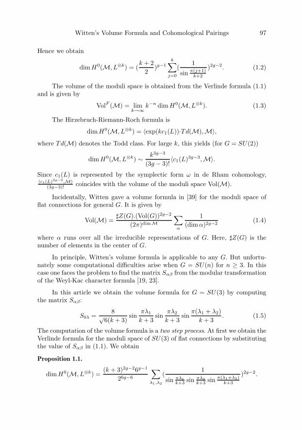
Witten’s Volume Formula and Cohomological Pairings 97
Hence we obtain
dimH0(M, L⊗k) = (k + 2
2)g−1
k∑j=0
(1
sin π(j+1)k+2
)2g−2. (1.2)
The volume of the moduli space is obtained from the Verlinde formula (1.1)and is given by
VolF (M) = limk→∞
k−n dimH0(M, L⊗k). (1.3)
The Hirzebruch-Riemann-Roch formula is
dimH0(M, L⊗k) = 〈exp(kc1(L))·Td(M),M〉,where Td(M) denotes the Todd class. For large k, this yields (for G = SU(2))
dimH0(M, L⊗k) ∼ k3g−3
(3g − 3)!〈c1(L)3g−3,M〉.
Since c1(L) is represented by the symplectic form ω in de Rham cohomology,〈c1(L)3g−3,M〉
(3g−3)! coincides with the volume of the moduli space Vol(M).
Incidentally, Witten gave a volume formula in [39] for the moduli space offlat connections for general G. It is given by
Vol(M) =�Z(G).(Vol(G))2g−2
(2π)dimM∑α
1(dimα)2g−2
(1.4)
where α runs over all the irreducible representations of G. Here, �Z(G) is thenumber of elements in the center of G.
In principle, Witten’s volume formula is applicable to any G. But unfortu-nately some computational difficulties arise when G = SU(n) for n ≥ 3. In thiscase one faces the problem to find the matrix Sαβ from the modular transformationof the Weyl-Kac character formula [19, 23].
In this article we obtain the volume formula for G = SU(3) by computingthe matrix Sαβ :
S0λ =8√
6(k + 3)sin
πλ1
k + 3sin
πλ2
k + 3sin
π(λ1 + λ2)k + 3
. (1.5)
The computation of the volume formula is a two step process. At first we obtain theVerlinde formula for the moduli space of SU(3) of flat connections by substitutingthe value of Sαβ in (1.1). We obtain
Proposition 1.1.
dimH0(M, L⊗k) =(k + 3)2g−26g−1
26g−6
∑λ1,λ2
(1
sin πλ1k+3 sin πλ2
k+3 sin π(λ1+λ2)k+3
)2g−2.

98 Partha Guha
In the next step, using the above formula and Witten’s prescription for largek limit, we obtain the volume of the moduli space of flat SU(3) connections; thisyields
Proposition 1.2.
Vol(M)SU(3)) = 36g−1
(2π)6g−6
∞∑n1,n2
n−(2g−2)1 n
−(2g−2)2 (n1 + n2)−(2g−2).
Here, a multiple zeta function appears in the volume of flat SU(3) connectionsVol(M)SU(3):
ζg(A, 2g − 2) =∞∑
n1,n2
1n2g−2
1 n2g−22 (n1 + n2)2g−2
. (1.6)
It is a member of a family of a much larger class of zeta functions, known as multiplezeta functions. The Euler-Zagier multiple zeta functions are nested generalizationsof the Riemann zeta function [37, 38]. They are defined as
ζk(s1, . . . , sk) =∑
0<n1<···<nk
n−s11 · · ·n−sk
k .
Here, s1, · · · , sk ∈ Z, s1 ≥ 2, sj ≥ 1 for 2 ≤ j ≤ k. For k = 1 this reduces toRiemann’s zeta function. We call k the length or depth of s and |s| =
∑sj the
weight of s.Unlike as for the Riemann zeta function one could determine several algebraic
relations between the multiple zeta values (MZV). One type of such relationsappears when one multiplies two such series. In fact, one gets a linear combinationof MZV. A simple example is stated below:
ζ(s)ζ(s′) =∑n≥1
1ns
∑m≥1
1ms′
=∑n>m
+∑n<m
+∑n=m
= ζ(s, s′) + ζ(s′, s) + ζ(s + s′).
This is a quadratic relation among zeta values. In general the quadratic relationis given as
ζ(s)ζ(s′) =∑
σ
σ.
This manipulation leads to the definition of a product called stuffle product [6].This is a formal sum defined recursively by
aP ∗ bQ = a(P ∗ bQ) + b(aP ∗Q) + (a + b)(P ∗Q).
A simple example is
ζ(s)2 = 2ζ(s, s) + ζ(2s).

Witten’s Volume Formula and Cohomological Pairings 99
Then for s = 2, ζ(2) = π2/6 and ζ(4) = π4/90, we obtain
ζ(2, 2) =∑
m>n≥1
(mn)−2 =π4
120.
Another example is ζ(2)ζ(3) = ζ(2, 3) + ζ(3, 2) + ζ(5).
Remark. In the same way as the stuffle product arises in the reorganization ofmultiple sums, multiple integrals lead to the definition of the shuffle product ofwords over an alphabet (with two letters) X = {x0, x1}. The words are given asX∗ = {xa1
0 xb11 · · ·xak
0 xbk1 }. This product is defined by the same formula as the
stuffle product except that the last term in the sum is omitted. The algebraicrelations between multiple polylogarithms
Li(s1···sk)(z) =∑
n1>n2>···nk≥1
zn1
ns11 · · ·nsk
k
|z| < 1 ∀sj ≥ 1
is generated by the shuffle relation. In fact, these multiple polylogarithms can beexpressed as iterated Chen integrals, and from this representation one obtains theshuffle relations (for an example, see [7]).
In our case, Zagier [41, 42] gave a formula for calculating the values of thisparticular multiple zeta function. This result is also derived using the stuffle prod-uct. The key formula to compute our volume form is given by
∞∑m,n
1msns(m + n)s
=43
∑0≤r≤s; r even
(2s− r − 1
s− 1
)ζ(r)ζ(3s − r). (1.7)
Witten’s volume formula can be extended to the moduli space of vector bun-dles with marked points z1, z2, . . . , zp ∈ Σg. We associate to each marked pointzi an irreducible representation Γ of GC. If λ is the highest weight of Γ, then(λ, αmax) ≤ k where αmax is the highest root and ( , ) is the basic inner product(see appendix, [23]): alternatively λ is in the fundamental domain of the actionof the affine Weyl group at level k + h on the Cartan subalgebra (Lie algebra ofthe maximal torus). We sum over representations Γ for which, if λ is the highestweight of Γλ, the representation of dimension (n + 1) and all the marked pointsare labeled by Γnr . We associate a complex vector space to each labeled Riemannsurface.
The generalized Verlinde formula for a group G in the presence of markedpoints [39] is
dimH0(MG, L⊗k ⊗
⊗iΓni) =
k∑j=0
1S2g−2+p
0,j
p∏i=1
Sni,j (1.8)
and the vector space H0(MG, L⊗k ⊗⊗
iΓni) is independent of the details of thepositions of the marked points.

100 Partha Guha
Similarly, the volume of the generalized moduli space can be obtained fromthis generalized Verlinde formula (1.8) by extracting the term at the large k limit(1.3).
The volume formula for G = SU(2) with marked points is given as
VolF (Mt) = 2.1
2g−1π2g−2+p
p∑n=1
∏pi=1 sin(πnti)n2g−2+p
. (1.9)
Our strategy is to compute the volume using the Verlinde formula in thelarge k limit rather than using Witten’s volume formula directly, and this will beour recipe to find the volume of the moduli space.
Unlike the SU(2) case, we obtain the volume formula for the moduli spaceof flat SU(3) connections in terms of multiple zeta functions or double Bernoullinumbers [4, 5].
We obtain the volume formula of the moduli space of flat SU(3) connectionsover one marked point Riemann surface.
Proposition 1.3.
VolF (Mt) =3.6g−1
26g−6π6g−3
∑ sinπn1t1. sinπn2t2. sinπ(n1 + n2)(t1 + t2)n2g−1
1 n2g−12 (n1 + n2)2g−1
t1 and t2 are restricted to
0 < ti < 1.
When we expand the sine terms, we obtain a comprehensive volume formula forfinding the intersection pairings of moduli space.
Witten’s idea is based on the symplectic volume of the moduli space of flatconnections. The moduli space M of flat connections of any semi-simple group Gis a symplectic variety with a symplectic form ω. The volume of the moduli spaceof flat SU(n) connections is
VolS(M) =1r!
∫M
ωr,
where r = (n2 − 1)(g − 1) = (g − 1) dimG is the dimension of the moduli space.Witten showed in [39] that the Reidemeister torsion of a Riemann surface,
equipped with a flat connection, determines a natural volume form on the modulispace of flat connections, which agrees with the symplectic volume. Given a chaincomplex C• that computes H∗(Σ, ad(E)), we define the torsion τ(C•) as a vectorin
(detH0(Σ, ad(E)))−1 ⊗ detH1(Σ, ad(E))⊗ detH2(Σ, ad(E)))−1.
For an irreducible flat connection:
H0(Σ, ad(E)) = H2(Σ, ad(E)) = 0.
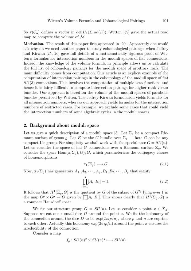
Witten’s Volume Formula and Cohomological Pairings 101
So τ(C•) defines a vector in detH1(Σ, ad(E)). Witten [39] gave the actual roadmap to compute the volume of M.
Motivation. The result of this paper first appeared in [20]. Apparently one wouldask why do we need another paper to study cohomological pairings, when Jeffreyand Kirwan [25, 26] gave full details of a mathematically rigorous proof of Wit-ten’s formulas for intersection numbers in the moduli spaces of flat connections.Indeed, the knowledge of the volume formula in principle allows us to calculatethe full list of cohomology pairings for the moduli space of arbitrary rank. Themain difficulty comes from computation. Our article is an explicit example of thecomputation of intersection pairings in the cohomology of the moduli space of flatSU(3) connections. This involves the computation of multiple zeta functions andhence it is fairly difficult to compute intersection pairings for higher rank vectorbundles. Our approach is based on the volume of the moduli spaces of parabolicbundles prescribed by Witten. The Jeffrey-Kirwan formulation yields formulas forall intersection numbers, whereas our approach yields formulas for the intersectionnumbers of restricted cases. For example, we exclude some cases that could yieldthe intersection numbers of some algebraic cycles in the moduli spaces.
2. Background about moduli space
Let us give a quick description of a moduli space [3]. Let Σg be a compact Rie-mann surface of genus g. Let E be the G bundle over Σg — here G can be anycompact Lie group. For simplicity we shall work with the special case G = SU(n).Let us consider the space of flat G connections over a Riemann surface Σg. Weconsider the space Hom(π(Σg), G)/G, which parameterizes the conjugacy classesof homomorphisms
π1(Σg) −→ G. (2.1)
Now, π1(Σg) has generators A1, A2, · · · , Ag, B1, B2, · · · , Bg that satisfyg∏
i=1
[Ai, Bi] = 1. (2.2)
It follows that H1(Σg, G) is the quotient by G of the subset of G2g lying over 1 inthe map Gg ×Gg → G given by
∏[Ai, Bi]. This shows clearly that H1(Σg, G) is
a compact Hausdorff space.
We fix our structure group G = SU(n). Let us consider a point x ∈ Σg.Suppose we cut out a small disc D around the point x. We fix the holonomy ofthe connection around the disc D to be exp(2πip/n), where p and n are coprimeto each other. Actually this holonomy exp(2πip/n) around the point x ensures theirreducibility of the connection.
Consider a map
fg : SU(n)g × SU(n)g �−→ SU(n)

102 Partha Guha
defined by
(A1, B1, . . . , Ag, Bg) �−→g∏i
AiBiA−1i B−1
i .
In particular we select the subspace Wg = f−1g (exp(2πip/n) of SU(n)2g.
A point, say x, in the space SU(n)g×SU(n)g is considered to be reducible ifthere exists a matrix T in SU(n) such that (TAiT
−1, TBiT−1 . . .) are all diagonal.
When n > 2, we should include also those points where there exist matrices thatcan be simultaneously block diagonalized, for example, in the case of SU(3) thiswould go into S(U(2)×U(1)). If x is a reducible point of SU(n)2g, then fg(x) = I,so the connections take values in the Abelian subgroup of SU(n).
Now it follows that the diagonal conjugation action of SU(n)/Z(G) = PU(n)(where Z(G) is the center of SU(n)) on SU(n)2g clearly preserves Wg and alsoby Schur’s Lemma that the restriction of the action is free. Hence, the quotientWg/PU(n) is a smooth compact Hausdorff space, it is a manifold of dimension2(g − 1) dimG at all irreducible points (i.e. when the image of π1(Σ) generates G).
We can give an equivalent description of this moduli space in the holomorphicway (see [2, 21, 22]). The space of connections A over E is an affine space modeledon Ω1(Σg, adE), such that the tangent space of A at any point is canonicallyidentified with Ω1(Σg, adE). Let us consider a decomposition of
Ω1(Σg, adE)⊗C = Ω1,0(Σg, adEC)⊕ Ω0,1(Σg, adEC).
If we consider an isomorphism between Ω1(Σg, adE) and Ω0,1(Σg, adEC), we ob-tain a complex structure on the modeled space of A and hence also on A. Wesay that A is the space of ∂ operators on EC . In the holomorphic picture wemust restrict to a stable bundle [30] in order to obtain a smooth moduli space.A holomorphic vector bundle E is semi-stable over a Riemann surface, if for allsub-bundles F it satisfies
degF
rankF≤ degE
rankE.
Here, “degree” stands for the value of the first Chern class. The vector bundle Eis a stable bundle if this inequality is strict. When the degree and the rank arecoprime, then all the semi-stable bundles are stable. In this holomorphic picturethe moduli space is interpreted as the space of gauge equivalence classes of stablevector bundles, i.e.M(Σ, G) = AS/GC , where Aut(EC) = GC acts onAS with theconstant scalars as the only isotropy group. The celebrated theorem of Narasimhanand Seshadri [31] connects both the pictures and it states that stable bundlesarising from the representations of π1 give irreducible representations.
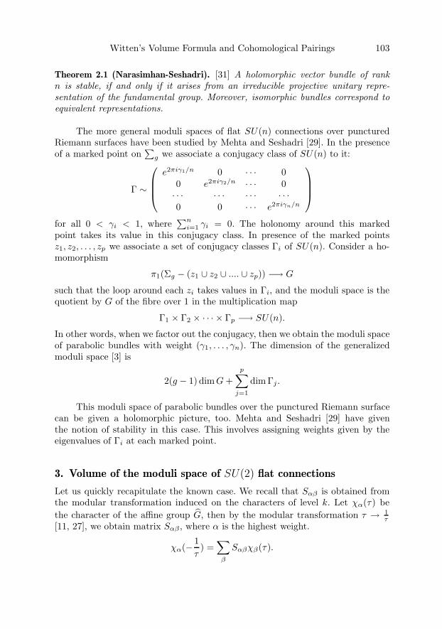
Witten’s Volume Formula and Cohomological Pairings 103
Theorem 2.1 (Narasimhan-Seshadri). [31] A holomorphic vector bundle of rankn is stable, if and only if it arises from an irreducible projective unitary repre-sentation of the fundamental group. Moreover, isomorphic bundles correspond toequivalent representations.
The more general moduli spaces of flat SU(n) connections over puncturedRiemann surfaces have been studied by Mehta and Seshadri [29]. In the presenceof a marked point on
∑g we associate a conjugacy class of SU(n) to it:
Γ ∼
⎛⎜⎜⎝e2πiγ1/n 0 · · · 0
0 e2πiγ2/n · · · 0· · · · · · · · · · · ·0 0 · · · e2πiγn/n
⎞⎟⎟⎠for all 0 < γi < 1, where
∑ni=1 γi = 0. The holonomy around this marked
point takes its value in this conjugacy class. In presence of the marked pointsz1, z2, . . . , zp we associate a set of conjugacy classes Γi of SU(n). Consider a ho-momorphism
π1(Σg − (z1 ∪ z2 ∪ .... ∪ zp)) −→ G
such that the loop around each zi takes values in Γi, and the moduli space is thequotient by G of the fibre over 1 in the multiplication map
Γ1 × Γ2 × · · · × Γp −→ SU(n).
In other words, when we factor out the conjugacy, then we obtain the moduli spaceof parabolic bundles with weight (γ1, . . . , γn). The dimension of the generalizedmoduli space [3] is
2(g − 1) dimG +p∑
j=1
dim Γj.
This moduli space of parabolic bundles over the punctured Riemann surfacecan be given a holomorphic picture, too. Mehta and Seshadri [29] have giventhe notion of stability in this case. This involves assigning weights given by theeigenvalues of Γi at each marked point.
3. Volume of the moduli space of SU(2) flat connections
Let us quickly recapitulate the known case. We recall that Sαβ is obtained fromthe modular transformation induced on the characters of level k. Let χα(τ) bethe character of the affine group G, then by the modular transformation τ → 1
τ[11, 27], we obtain matrix Sαβ , where α is the highest weight.
χα(−1τ) =
∑β
Sαβχβ(τ).
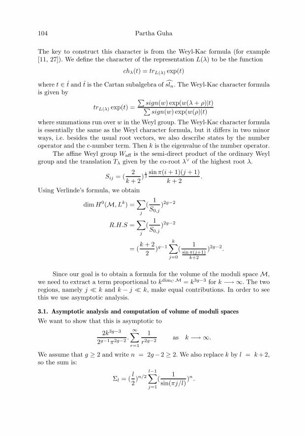
104 Partha Guha
The key to construct this character is from the Weyl-Kac formula (for example[11, 27]). We define the character of the representation L(λ) to be the function
chλ(t) = trL(λ) exp(t)
where t ∈ t and t is the Cartan subalgebra of sln. The Weyl-Kac character formulais given by
trL(λ) exp(t) =∑
sign(w) exp(w(λ + ρ)|t)∑sign(w) exp(w(ρ)|t)
where summations run over w in the Weyl group. The Weyl-Kac character formulais essentially the same as the Weyl character formula, but it differs in two minorways, i.e. besides the usual root vectors, we also describe states by the numberoperator and the c-number term. Then k is the eigenvalue of the number operator.
The affine Weyl group Waff is the semi-direct product of the ordinary Weylgroup and the translation Tλ given by the co-root λ∨ of the highest root λ.
Sij = (2
k + 2)
12sinπ(i + 1)(j + 1)
k + 2.
Using Verlinde’s formula, we obtain
dimH0(M, Lk) =∑
j
(1
S0,j)2g−2
R.H.S =∑
j
(1
S0,j)2g−2
= (k + 2
2)g−1
k∑j=0
(1
sin π(j+1)k+2
)2g−2.
Since our goal is to obtain a formula for the volume of the moduli space M,we need to extract a term proportional to kdimC M = k3g−3 for k −→∞. The tworegions, namely j % k and k − j % k, make equal contributions. In order to seethis we use asymptotic analysis.
3.1. Asymptotic analysis and computation of volume of moduli spaces
We want to show that this is asymptotic to
2k3g−3
2g−1π2g−2.
∞∑r=1
1r2g−2
as k −→∞.
We assume that g ≥ 2 and write n = 2g−2 ≥ 2. We also replace k by l = k+2,so the sum is:
Σl = (l
2)n/2
l−1∑j=1
(1
sin(πj/l))n.

Witten’s Volume Formula and Cohomological Pairings 105
We divide this sum into the combination from j ≤ l/2, j ≥ l/2: these are essentiallythe same, hence it suffices to treat the first one. For ε > 0, we write
l/2∑j=1
(1
sinπj/l)n =
[εl]∑j=1
(1
sinπj/l)n +
l/2∑[εl]+1
(1
sinπj/l)n
= S + T, say .
We want to compare the sum S with S′ =∑∞
j=1(l
πj )n. The difference S−S′ arisesfrom two factors – approximating the sin function by its derivative and changingthe range of summation. For the first case we have, for small ε and j/l < ε,
πj/l ≥ sin(πj/l) ≥ πj/l− 1/6(πj/l)3.
This implies that, for some constant C,
(l
πj)n ≤ (
1sin(πj/l)
)n ≤ (kn
πj)n(1 + C(
j
l)2).
So
|[εl]∑j=1
(1
sin(πjl )
)n −[εl]∑j=1
(l
πj)n| ≤ C
εl∑j=1
ln−2
jn−2≤ C′ln−1,
for some C′ (since these are O(l) terms in the sum).For the second factor:
∞∑j=1
(l
πj)n −
[εl]∑j=1
(l
πj)n =
∞∑[εl]+1
(l
πj)n = O(ln−1)
by comparing with the integral∫∞
εl x−ndx. Hence, we see that S − S′ is O(ln−1).Finally consider the other term T :
T =l/2∑
[εl]+1
(1
sin(πj/l))n.
In this sum
sin(πj/l) ≥ δ(ε)
say so, for fixed ε, T = O(l) (the number of terms in the sum). Putting all ofthis together, we see that
Σl = (l
2)n/2.(2
∞∑j=1
(l
πj)n + O(ln−1),
which gives the required result.

106 Partha Guha
Hence, for large k we obtain
dimH0(M, Lk) ∼ 2(k + 2
2)g−1
k∑j=0
(k + 2
π(j + 1))2g−2
= 2k3g−3
2g−1π2g−2
∞∑n=1
1n2g−2
.
This finally yields
dimH0(M, Lk) = 2k3g−3
2g−1π2g−2ζ(2g − 2). (3.1)
From the algebraic geometry point of view this dimension can be expressedvia the Hirzebruch-Riemann-Roch theorem [18]
dimH0(M, Lk) = 〈exp(kc1(L)).T d(M),M〉and for large k,
dimH0(M, Lk) ∼ k3g−3
(3g − 3)!〈c1(L)3g−3,M〉. (3.2)
Now c1(L) is represented by the symplectic form ω in de Rham cohomology. Hence
〈c1(L)3g−3,M〉(3g − 3)!
coincides with Vol(M). Equating the expressions (3.1) and (3.2), we obtain
Vol(M) = 21
(2π2)g−1
∞∑n=1
n−(2g−2)
= 2ζ(2g − 2)(2π2)g−1
This is known as Witten’s volume formula [39] of the moduli space of flat SU(2)connections.
4. Volume of the moduli space of flat SU(3) connections
We first recall some definitions of affine SU(3) characters (for example [11, 27]).The affine SU(3) characters are labeled by a highest weight Λ = λ1Λ1+λ2Λ2 wherethe Λi’s are the fundamental weights and the set of components {λi} contains non-negative integers. If the height of affine SU(3) is n = k + 3 with level k ≥ 0, thehighest weights corresponding to unitary representations satisfy λ1+λ2 ≤ k. Thus,there are (k+1)(k+2)
2 = (n−1)(n−2)2 independent affine characters. To see these more
explicitly, let us consider shifted weight λ = Λ+Λ1 +Λ2 = p1Λ1 +p2Λ2. Unitarityof the representations implies that λ belongs to the fundamental domain W ,
W = {λ = p1Λ1 + p2Λ2, pi ≥ 1 and p1 + p2 ≤ n− 1},
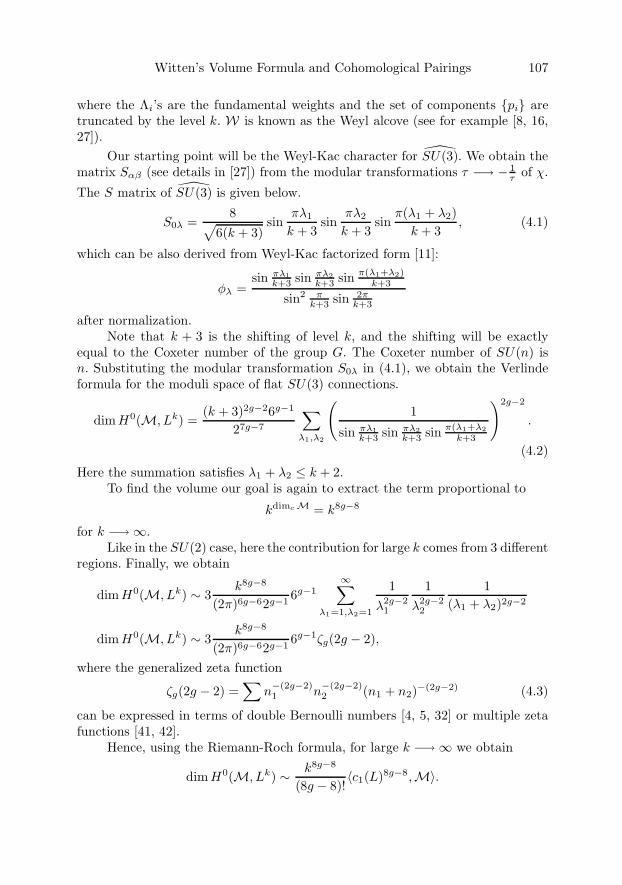
Witten’s Volume Formula and Cohomological Pairings 107
where the Λi’s are the fundamental weights and the set of components {pi} aretruncated by the level k. W is known as the Weyl alcove (see for example [8, 16,27]).
Our starting point will be the Weyl-Kac character for SU(3). We obtain thematrix Sαβ (see details in [27]) from the modular transformations τ −→ − 1
τ of χ.
The S matrix of SU(3) is given below.
S0λ =8√
6(k + 3)sin
πλ1
k + 3sin
πλ2
k + 3sin
π(λ1 + λ2)k + 3
, (4.1)
which can be also derived from Weyl-Kac factorized form [11]:
φλ =sin πλ1
k+3 sin πλ2k+3 sin π(λ1+λ2)
k+3
sin2 πk+3 sin 2π
k+3
after normalization.Note that k + 3 is the shifting of level k, and the shifting will be exactly
equal to the Coxeter number of the group G. The Coxeter number of SU(n) isn. Substituting the modular transformation S0λ in (4.1), we obtain the Verlindeformula for the moduli space of flat SU(3) connections.
dimH0(M, Lk) =(k + 3)2g−26g−1
27g−7
∑λ1,λ2
(1
sin πλ1k+3 sin πλ2
k+3 sin π(λ1+λ2k+3
)2g−2
.
(4.2)
Here the summation satisfies λ1 + λ2 ≤ k + 2.To find the volume our goal is again to extract the term proportional to
kdimc M = k8g−8
for k −→∞.Like in the SU(2) case, here the contribution for large k comes from 3 different
regions. Finally, we obtain
dimH0(M, Lk) ∼ 3k8g−8
(2π)6g−62g−16g−1
∞∑λ1=1,λ2=1
1λ2g−2
1
1λ2g−2
2
1(λ1 + λ2)2g−2
dimH0(M, Lk) ∼ 3k8g−8
(2π)6g−62g−16g−1ζg(2g − 2),
where the generalized zeta function
ζg(2g − 2) =∑
n−(2g−2)1 n
−(2g−2)2 (n1 + n2)−(2g−2) (4.3)
can be expressed in terms of double Bernoulli numbers [4, 5, 32] or multiple zetafunctions [41, 42].
Hence, using the Riemann-Roch formula, for large k −→∞ we obtain
dimH0(M, Lk) ∼ k8g−8
(8g − 8)!〈c1(L)8g−8,M〉.

108 Partha Guha
Again, c1(L) is represented by the symplectic form ω and the term
〈c1(L)8g−8,M〉(8g − 8)!
coincides with Vol(M). Hence we obtain
Vol(M)SU(3) = 36g−1
(2π)6g−62g−1ζg(2g − 2).
Finally, using the formula [42] of the multiple zeta function∞∑
m,n
1msns(m + n)s
=43
∑0≤r≤s;reven
(2s− r − 1
s− 1
)ζ(r)ζ(3s − r)
we obtain following examples.
Example : For g = 2 we know the value of the zeta function from Zagier [41, 42]:ζ2(2) = (2π)6/7! 36. So the volume is
Vol(M) = 3.6
(2π)6.2.(2π)6
7! 36. = 1/4.7!
This is the first generalization of Witten’s result [39] for the moduli space of SU(2)flat connections to the moduli space of flat SU(3) connections.
5. Cohomological pairings of the moduli space
This is the central theme of the whole article. Our goal here is to find out thecohomological pairings of the moduli space of flat SU(3) connections on the Rie-mann surface. Our recipe to find the volume will be to use a generalized Verlindeformula (for the marked point case) (1.8) in the large k-limit. This volume formulacontains all the information of certain cohomological pairings.
5.1. Review of Donaldson-Thaddeus-Witten’s work on SU(2) moduli space
Let M1 be the moduli space of flat SU(2) connections. For a rational number0 < t < 1, we consider Mt to be the moduli space of flat connections on Σg − x,such that monodromy around x is in the conjugacy classes of SU(2)
T =(
exp(iπt) 00 exp(−iπt)
).
One can show that for t close to 1, Mt is a CP 1 bundle over the moduli spaceM1.
CP1 −−−−→ Mt⏐⏐.M1
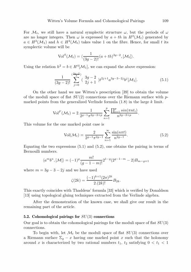
Witten’s Volume Formula and Cohomological Pairings 109
For Mt, we still have a natural symplectic structure ω, but the periods of ωare no longer integers. Then ω is expressed by a + th in H2(Mt) generated bya ∈ H2(M1) and h ∈ H2(Mt) takes value 1 on the fibre. Hence, for small t itssymplectic volume will be
VolS(Mt) = 〈 1(3g − 2)!
(a + th)3g−2, [Mt]〉.
Using the relation h2 = b ∈ H4[M1], we can expand the above expression:
1(3g − 2)!
( 3g−22 )∑
j=0
(3g − 22j + 1 )t2j+1a3g−3−2jbj[M1]. (5.1)
On the other hand we use Witten’s prescription [39] to obtain the volumeof the moduli space of flat SU(2) connections over the Riemann surface with p-marked points from the generalized Verlinde formula (1.8) in the large k limit.
VolF (Mt) = 2.1
2g−1π2g−2+p
p∑n=1
∏pi=1 sin(πnti)n2g−2+p
.
This volume for the one marked point case is
Vol(Mt) =2
2g−1π2g−1
∞∑n=1
sin(nπt)n2g−1
. (5.2)
Equating the two expressions (5.1) and (5.2), one obtains the pairing in terms ofBernoulli numbers.
〈ambn, [M]〉 = (−1)g m!(g − 1−m)!
21−g(2g−1−m − 2)Bm−g+1
where m = 3g − 3− 2j and we have used
ζ(2k) =(−1)k+1(2π)2k
2.(2k)!B2k.
This exactly coincides with Thaddeus’ formula [33] which is verified by Donaldson[13] using topological gluing techniques extracted from the Verlinde algebra.
After the demonstration of the known case, we shall give our result in theremaining part of the article.
5.2. Cohomological pairings for SU(3) connections
Our goal is to obtain the cohomological pairings for the moduli space of flat SU(3)connections.
To begin with, let Mt be the moduli space of flat SU(3) connections overa Riemann surface Σg − x having one marked point x such that the holonomyaround x is characterized by two rational numbers t1, t2 satisfying 0 < t1 < 1
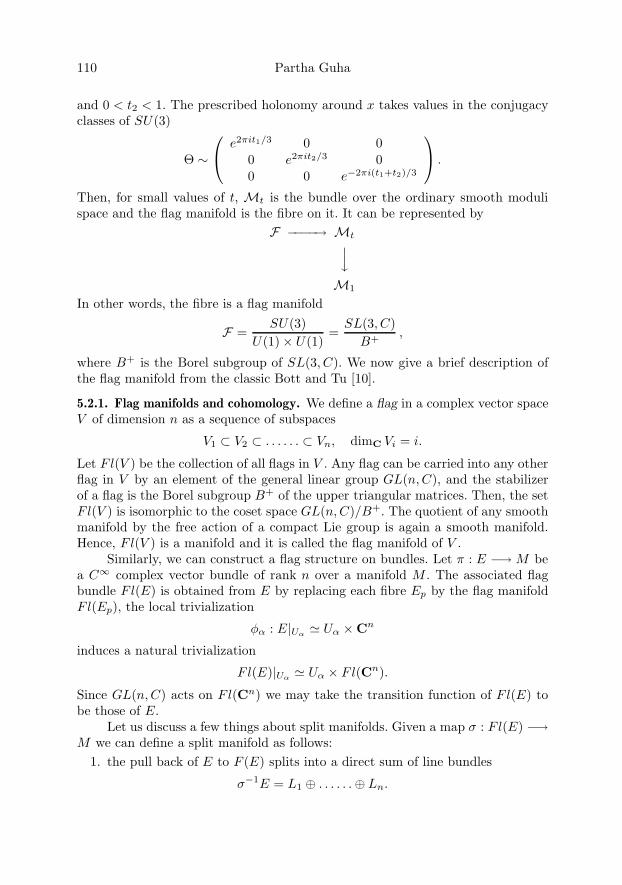
110 Partha Guha
and 0 < t2 < 1. The prescribed holonomy around x takes values in the conjugacyclasses of SU(3)
Θ ∼
⎛⎝ e2πit1/3 0 00 e2πit2/3 00 0 e−2πi(t1+t2)/3
⎞⎠ .
Then, for small values of t, Mt is the bundle over the ordinary smooth modulispace and the flag manifold is the fibre on it. It can be represented by
F −−−−→ Mt⏐⏐.M1
In other words, the fibre is a flag manifold
F =SU(3)
U(1)× U(1)=
SL(3, C)B+
,
where B+ is the Borel subgroup of SL(3, C). We now give a brief description ofthe flag manifold from the classic Bott and Tu [10].
5.2.1. Flag manifolds and cohomology. We define a flag in a complex vector spaceV of dimension n as a sequence of subspaces
V1 ⊂ V2 ⊂ . . . . . . ⊂ Vn, dimC Vi = i.
Let Fl(V ) be the collection of all flags in V . Any flag can be carried into any otherflag in V by an element of the general linear group GL(n,C), and the stabilizerof a flag is the Borel subgroup B+ of the upper triangular matrices. Then, the setFl(V ) is isomorphic to the coset space GL(n,C)/B+. The quotient of any smoothmanifold by the free action of a compact Lie group is again a smooth manifold.Hence, Fl(V ) is a manifold and it is called the flag manifold of V .
Similarly, we can construct a flag structure on bundles. Let π : E −→M bea C∞ complex vector bundle of rank n over a manifold M . The associated flagbundle Fl(E) is obtained from E by replacing each fibre Ep by the flag manifoldFl(Ep), the local trivialization
φα : E|Uα � Uα ×Cn
induces a natural trivialization
Fl(E)|Uα � Uα × Fl(Cn).
Since GL(n,C) acts on Fl(Cn) we may take the transition function of Fl(E) tobe those of E.
Let us discuss a few things about split manifolds. Given a map σ : Fl(E) −→M we can define a split manifold as follows:
1. the pull back of E to F (E) splits into a direct sum of line bundles
σ−1E = L1 ⊕ . . . . . .⊕ Ln.

Witten’s Volume Formula and Cohomological Pairings 111
2. σ∗ embeds H∗(M) in H∗(Fl(E)).The split manifold Fl(E) is obtained by a sequence of n− 1 projectivization. Weshall now apply all these to obtain cohomology rings of flag manifolds.
Proposition 5.1. The associated flag bundle Fl(E) of a vector bundle is the splitmanifold.
Proof: Given in Bott [10] (chapter 4). �If E is a rank n complex vector bundle over M , then the cohomology ring of
its projectivization is
H∗(P (E)) = H∗(M)[c1, . . . , cn, d1, . . . , dn]/{C(S)C(Q) = π∗C(E)},where c1, ....., cn are the Chern classes of the universal subbundle S and d1, ......, dn
are the classes of the universal quotient bundle Q. Also C(S) and C(Q) denote thetotal Chern classes of S and Q. respectively. The flag manifold is obtained from asequence of (n− 1) projectivizations
H∗(Fl(E))
= H∗(M)[C(S1), ...., C(Sn−1), C(Q1, ....., Qn−1)]/C(S1)...C(Sn−1)C(Qn−1)
= C(E).
If
hi = C1(Si), i = 1...n− 1
hn = C(Qn−1),
then we have
H∗(Fl(E)) = H∗(M)[h1, .., hn]/(n∏
i=1
(1 + hi)) = C(E)).
In order to obtain the cohomology ring of the flag manifold F [10], we have toconsider a trivial bundle over a point.
H∗(F ) = R[h1, ..., hn]/(n∏
i=1
(1 + hi) = 1).
For the special case n = 3, we obtain
H∗(F ) = R[h1, h2, h3]/(3∏
i=1
(1 + hi) = 1).
5.2.2. Computation of the intersection pairings. We are going to apply our pre-vious scheme. Since Mt is a bundle over M1, we can pull back the cohomologyfrom the base manifold M1. In fact, it is not hard to see that the symplectic formω represents the class
a + t1h1 + t2h2 ∈ H2(Mt),

112 Partha Guha
where a ∈ H2(M1) and hi ∈ H2(Mt). So from this symplectic form the volumewill be the following
VolS(Mt) = 〈 1(8g − 5)!
(a + t1h1 + t2h2)8g−5, [Mt]〉.
When we expand this expression, then we obtain the following results.
Proposition 5.2.
VolS(Mt) =∑k,l
1(8g − 5− k − l)!k!l!
tk1tl2〈a8g−5−k−lhk
1hl2, [Mt]〉.
But to get the exact pairing, we have to use the knowledge of Witten’s volumefunction for small t1, t2, and also we use the following identities viz.
h21 = b ∈ H4; h2
2 = c ∈ H4; −h1h2 = d ∈ H4
h21h2 = e ∈ H6; −h2
2h1 = f ∈ H6.
Note that h21h2 = −h1h
22 is a fundamental class of the Flag manifold, these are
top cohomology modules. The key lemma for obtaining the cohomology ring overthe moduli space M1 follows from the Leray-Hirsch theorem [10].
Theorem 5.3. (Leray-Hirsch) Let E be a fibre bundle over a manifold M withfibre F . Assume M has finite good cover and suppose there are global cohomologyclasses e1, e2, . . . , er on E which – when restricted to each fibre – freely generatethe cohomology of the fibre. Then H∗(E) is a free module over H∗(M) with basis{e1, e2, . . . , er}, i.e.
H∗(E) ∼= H∗(M)⊗R[e1, e2, ....., er]∼= H∗(M)⊗H∗(F).
Now we formulate an important statement.
Lemma 5.4. The fundamental classes of Mt are the product of the fundamentalclasses of the moduli space without marked point M1 and the fundamental classesof the flag manifold.
We use the same recipe, i.e., extracting the volume from the generalizedVerlinde formula (1.8), to find the volume of the moduli space.
If we feed the value of Sαβ of SU(3) obtained from the modular transfor-mation of the Weyl-Kac character into the Verlinde formula (1.8) and repeat thederivation as in the previous section, we obtain the torsion volume
VolF (Mt) =3.6g−1
27g−7π6g−3
∑ sinπn1t1 sinπn2t2 sinπ(n1 + n2)(t1 + t2)n2g−1
1 n2g−12 (n1 + n2)2g−1
.
This is the generalization of Witten’s volume formula for the moduli space of flatSU(3) connections. It is the volume of the moduli space of flat SU(3) connectionsover a Riemann surface of genus g with one marked point.

Witten’s Volume Formula and Cohomological Pairings 113
After a tedious calculation which makes use of the Taylor expansion ofsinπn1t1, sinπn2t2 and sinπ(n1 + n2)(t1 + t2), the above expression for smallt1, t2 gives us a comprehensive formula:
Proposition 5.5.
Vol(Mt) =3.6g−1
27g−7π6g−3
∑n
∑j
×
(−1)j1+j2+j3π2j1+2j2+j3t2(j1+j3−j4)+11 t
2(j2+j4)+22
(2j1 + 1)!(2j2 + 1)!(2j3 − 2j4)!(2j4 + 1)!n2g−2j1−21 n2g−2j2−2
2 (n1 + n2)2g−2j3−2.
This is the key formula for getting the cohomology pairings of the modulispace of flat SU(3) connections, and is Witten’s volume formula for moduli spaceof flat SU(3) connections. This formula is too bigm but can be handled for somelower genus cases.
5.3. Concrete examples
It is clear that the two volumes of the moduli space, namely the symplectic volumeVolS(Mt) and the volume from Verlinde’s formula V ol(Mt) in claim (1.9) areequal.
Using this simple prescription we obtain explicit examples of the cohomologi-cal pairings of the moduli space of flat SU(3) connections. This pairing is expressedin terms of a multiple zeta function [41, 42] or double Bernoulli numbers [4, 5].Equating the powers of tk1t
l2 we obtain explicit pairings.
1. We consider genus = 3. Thus we obtain
〈a10e1f1[M]〉 =3.7!5!3!.22.8.9.10
28.(2π)6ζSU(3).
From Zagier’s formula we now come to know that the value of this functionis (2π)6./7!.36. Hence
〈a10e1f1[M]〉 = (10.9.3.6.2).(24.5!)/4.36.26 = 5.9.15 = 675.
2. Once again consider genus = 3. We obtain
〈a10f2[M]〉 =10.9.8.6.7!6!.22
(2π)6.282
ζ(2, A)
i.e.
〈a10f2[M]〉 = 10.9.8.5!.22/28 = 1350.
Thus, we gave two explicit examples of pairings. Indeed it is really hard tocompute any arbitrary higher genus pairings. We hope that our readers realize thedegree of complications for further computations of intersection pairings.

114 Partha Guha
Acknowledgement. First of all, the author would like to express his respectful grat-itude to his thesis advisor, Professor Simon Donaldson, for numerous suggestions,guidance and encouragement. He is also grateful to Professors Nigel Hitchin, PeterKronheimer and Michael Thaddeus for their valuable comments and suggestions.He is extremely grateful to Professor Don Zagier for his numerical help and forcalculating the expression of the multiple zeta function.
References
[1] T. Apostol, Introduction to Analytic Number theory. Springer-Verlag. 1976.
[2] M.F. Atiyah and R. Bott, The Yang-Mills equation over the Riemann surface. Phi-los.Trans. R.Soc.London A308,523–615. 1982.
[3] M.F. Atiyah. The Geometry and Physics of Knots. Cambridge University Press.1990.
[4] E.W. Barnes. The theory of the double gamma function. Phil.Trans. Roy-Soc.A 196,265–388.1901.
[5] E.W. Barnes. On the theory of the multiple gamma function. Trans. CambridgePhil.Soc 19,374–425. 1904.
[6] J.M. Borwein, D.M. Bradley and D.J. Broadhurst, Evaluations of k-fold Euler/Zagiersums: a compendium of results for arbitrary k. The Wilf Festschrift (Philadelphia,PA, 1996).
[7] D. Bowman and D.M. Bradley, Multiple polylogarithms: a brief survey. q-series withapplications to combinatorics, number theory, and physics (Urbana, IL, 2000), 71–92,Contemp. Math., 291, Amer. Math. Soc., Providence, RI, 2001. Electron. J. Combin.4 (1997), no. 2, Research Paper 5.
[8] R. Baston and M. Eastwood. The Penrose Transform , its interaction with Repre-sentation theory. Oxford University Press. 1989.
[9] A. Beauville and Y. Laszlo. Conformal blocks and generalized theta divisor. Comm.Math. Phys. 164, 385–419. 1994.
[10] R. Bott and L. Tu. Differential forms in Algebraic topology. G.T.M. 82 Springer-Verlag. 1982.
[11] P. Di Francesco. Integrable lattice models, graphs and modular invariant conformalfield theories. Int. J. Mod. Phys. A 7, 407–500, 1992.
[12] S.K. Donaldson. A new proof to Narasimhan Seshadri’s theorem. J. Diff. Geom. 18, 269–277, 1983.
[13] S.K. Donaldson. Gluing technique in the cohomology of Moduli space. in TopologicalMethods in Modern Mathematics, J. Milnor 60th birthday festschrift. Publish orPerish. 1992.
[14] R. Earl and F. Kirwan, Complete sets of relations in the cohomology rings of modulispaces of holomorphic bundles and parabolic bundles over a Riemann surface. Proc.London Math. Soc. (3) 89 (2004), no. 3, 570–622.
[15] G. Faltings. A proof of Verlinde’s formula. J. Alg. Geom. 3, 347–374, 1994.
[16] W. Fulton and J. Harris. Representation theory, A first Course. Springer-Verlag.1991.
Witten’s Volume Formula and Cohomological Pairings 115
[17] V. Guillemin and S. Sternberg. Symplectic techniques in Physics. Cambridge Univ.Press. 1984.
[18] P. Griffith and J. Harris. Principles of Algebraic geometry. Wiley Interscience. 1978.
[19] D. Gepner and E. Witten. String theory on group manifolds. Nucl. Phys. B278,493–549. Appendix A. 1986.
[20] P. Guha, Topics in the geometry of holomorphic vector bundles, Thesis, Oxford Uni-versity 1994.
[21] N.J. Hitchin. The symplectic geometry of moduli spaces of connection and geometricquantization. Prog. of Theo Phys. Suppl.No.102, 159–174. 1990.
[22] N.J. Hitchin. Flat connections and geometric quantization. Commn. Math. Phys.131, 347. 1990.
[23] L. Jeffrey. Chern-Simons-Witten invariants of lens spaces and the torus bundles, andthe semiclassical approximation. Commun. Math. Phys. 147, 563–604. 1992.
[24] L. Jeffrey. Extended moduli spaces of flat connections on Riemann surfaces. Math.Ann. 298, 667–698. 1994.
[25] L. Jeffrey and F. Kirwan.Intersection numbers in moduli spaces of holomorphic bun-dles on a Riemann surface. Elec. Res. Ann. AMS 1, 57–71. 1995;
[26] L. Jeffrey and F. Kirwan Intersection pairings in moduli spaces of vector bundlesof arbitrary rank over a Riemann surface. Ann. of Math. (2) 148 (1998), no. 1,109–196.
[27] V. Kac. Infinite dimensional Lie algebras. Cambridge University Press. 1990.
[28] S. Kumar, M.S. Narasimhan and A. Ramanathan. Infinite Grassmannian and modulispaces of G-bundles. Math. Ann. 300, 41–75. 1994.
[29] V.B. Mehta and C.S. Seshadri. Moduli of vector bundles on curves with parabolicstructures. Math. Ann. 248, 205–239. 1980.
[30] D. Mumford. Projective invariants and projective structures and application. Proc.Inst. Cong. Math. Institut Mittag-Leffler. 1962
[31] M.S. Narasimhan and C.S. Seshadri. Stable and unitary vector bundle on a compactRiemann surface. Ann. Math. 82, 540–567. 1965.
[32] T. Shintani. On special values of zeta function of totally real algebraic number fields.Proc. Int. Cong. of Maths. Acad. Sci. Fennica, Helsinki. 591–597. 1978.
[33] M. Thaddeus. Conformal field theory and Cohomology of the Moduli space of stablebundles. J.Diff.Geom. 35, 131–149. 1992.
[34] A. Tsuchiya, K. Ueno and Y. Yamada, Conformal field theory on universal familyof stable curves with gauge symmetry. Advanced Studies in Pure Math. vol. 19,Princeton Univ. Press, 459–566. 1989.
[35] V.S. Varadarajan. Lie groups, Lie Algebras and their Representations. Springer-Verlag. 1984.
[36] E. Verlinde. Fusion rules and modular transformations in 2D conformal field theory.Nucl.Phys B 300, 360–370. 1988.
[37] M. Waldschmidt, Valeurs zeta multiples: une introduction. Journal de Theorie desNombres de Bordeaux, 12.2 (2000), 581–595.
116 Partha Guha
[38] M. Waldschmidt, Multiple Polylogarithms: An Introduction. (full text) 12p. Num-ber Theory and Discrete Mathematics Hindustan Book Agency, 2002, 1–12 Editors:A.K. Agarwal, B.C. Berndt, C.F. Krattenthaler, Gary L. Mullen, K. Ramachandraand Michel Waldschmidt. Institut de Mathematiques de Jussieu, Prepublication 275(janvier 2001), 11 p.
[39] E. Witten. On Quantum gauge theories in two dimensions. Commn. Math. Phys.141, 153–209. 1991.
[40] E. Witten. Two dimensional gauge theories revisited. J. Geom. Phys. 9, 303–368.1992.
[41] D.B. Zagier. Private communication.
[42] D.B. Zagier. Values of Zeta functions and their Applications. First European Con-gress of Mathematics, 1992, Vol.II, Edited by A. Joseph et. al. Birkhauser Verlag,1994.
Partha GuhaMax Planck Institute for Mathematics in the SciencesInselstrasse 22DE–04103 Leipzig
and
S.N. Bose National Centre for Basic SciencesJD Block, Sector - III, Salt LakeIN–700098 Kolkatae-mail: [email protected] & [email protected]
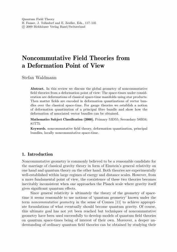
Quantum Field TheoryB. Fauser, J. Tolksdorf and E. Zeidler, Eds., 117–135c© 2009 Birkhauser Verlag Basel/Switzerland
Noncommutative Field Theories froma Deformation Point of View
Stefan Waldmann
Abstract. In this review we discuss the global geometry of noncommutativefield theories from a deformation point of view: The space-times under consid-eration are deformations of classical space-time manifolds using star products.Then matter fields are encoded in deformation quantizations of vector bun-dles over the classical space-time. For gauge theories we establish a notionof deformation quantization of a principal fibre bundle and show how thedeformation of associated vector bundles can be obtained.
Mathematics Subject Classification (2000). Primary 53D55; Secondary 58B34;81T75.
Keywords. noncommutative field theory, deformation quantization, principalbundles, locally noncommutative space-time.
1. Introduction
Noncommutative geometry is commonly believed to be a reasonable candidate forthe marriage of classical gravity theory in form of Einstein’s general relativity onone hand and quantum theory on the other hand. Both theories are experimentallywell-established within large regimes of energy and distance scales. However, froma more fundamental point of view, the coexistence of these two theories becomesinevitably inconsistent when one approaches the Planck scale where gravity itselfgives significant quantum effects.
Since general relativity is ultimately the theory of the geometry of space-time it seems reasonable to use notions of ‘quantum geometry’ known under theterm noncommutative geometry in the sense of Connes [11] to achieve appropri-ate formulations of what eventually should become quantum gravity. Of course,this ultimate goal has not yet been reached but techniques of noncommutativegeometry have been used successfully to develop models of quantum field theorieson quantum space-times being of interest of their own. Moreover, a deeper un-derstanding of ordinary quantum field theories can be obtained by studying their

118 Stefan Waldmann
counterparts on ‘nearby’ noncommutative space-times. On the other hand, peoplestarted to investigate experimental implications of a possible noncommutativityof space-time in future particle experiments.
Such a wide scale of applications and interests justifies a more conceptualdiscussion of noncommutative space-times and (quantum) field theories on them inorder to clarify fundamental questions and generic features expected to be commonto all examples.
In this review, we shall present such an approach from the point of view ofdeformation theory: noncommutative space-times are not studied by themselvesbut always with respect to a classical space-time, being suitably deformed intothe noncommutative one. Clearly, this point of view can not cover all possible(and possibly interesting) noncommutative geometries but only a particular class.Moreover, we focus on formal deformations for technical reasons. It is simplythe most easy approach where one can rely on the very powerful machinery ofalgebraic deformation theory. But it also gives hints on approaches beyond formaldeformations: finding obstructions in the formal framework will indicate even moresevere obstructions in any non-perturbative approach.
In the following, we discuss mainly two questions: first, what is the appro-priate description of matter fields on deformed space-times and, second, what arethe deformed analogues of principal bundles needed for the formulation of gaugetheories. The motivation for these two questions should be clear.
The review is organized as follows: in Section 2, we recall some basic def-initions and properties concerning deformation quantizations and star productsneeded for the set-up of noncommutative space-times. We discuss some funda-mental examples as well as a new class of locally noncommutative space-times.Section 3 is devoted to the study of matter fields: we use the Serre-Swan theoremto relate matter fields to projective modules and discuss their deformation theory.Particular interest is put on the mass terms and their positivity properties. InSection 4 we establish the notion of deformation quantization of principal fibrebundles and discuss the existence and uniqueness results. Finally, in Section 5 weinvestigate the resulting commutant and formulate an appropriate notion of as-sociated (vector) bundles. This way we make contact to the results of Section 3.The review is based on joint works with Henrique Bursztyn on one hand as wellas with Martin Bordemann, Nikolai Neumaier and Stefan Wei on the other hand.
2. Noncommutative space-times
In order to implement uncertainty relations for measuring coordinates of eventsin space-time it has been proposed already very early to replace the commuta-tive algebra of (coordinate) functions by some noncommutative algebra. In [17] aconcrete model for a noncommutative Minkowski space-time was introduced withcommutation relations of the form
[xμ, xν ] = iλθμν , (2.1)

Noncommutative Field Theories from a Deformation Point of View 119
where λ plays the role of the deformation parameter and has the physical dimensionof an area. Usually, this area will be interpreted as the Planck area. Moreover, θ isa real, antisymmetric tensor which in [17] and many following papers is assumedto be constant : in [17] this amounts to require that θμν belongs to the center ofthe new algebra of noncommutative coordinates. In fact, the approach in [17] wasmore subtle: the constants θμν are subject to a tensor transforming non-triviallyunder Lorentz transformations in such a way that the whole algebra is endowedwith a representation of the Lorentz (in fact Poincare) group by ∗-automorphisms.This was achieved by adding the whole Lorentz orbit of a constant tensor θμν withrank 4. Unfortunately, in the vast majority of the follow-up papers this feature ofLorentz invariance has been neglected. In the following we shall ignore symmetries,too, as in the end we focus on generic space-times without symmetries anyway.However, if there is a reasonably large symmetry group present, one can alwaysperform the construction parallel to [17] and add the orbit of the Poisson tensorunder the symmetry group.
Instead of constructing an abstract algebra where commutation relations like(2.1) are fulfilled, it is convenient to use a ‘symbol calculus’ and encode (2.1)already for the classical coordinate functions by changing the multiplication lawinstead. For functions f and g on the classical Minkowski space-time one definesthe Weyl-Moyal star product by
f � g = μ ◦ eiλ2 θμν ∂
∂xμ ⊗ ∂∂xν (f ⊗ g), (2.2)
where μ(f⊗g) = fg denotes the undeformed, pointwise product. Then (2.1) holdsfor the classical coordinate functions with respect to the �-commutator.
Clearly, one has to be slightly more careful with expressions like (2.2): inorder to make sense out of the infinite differentiations the functions f and g firstshould be C∞. But then the exponential series does not converge in general whencea more sophisticated analysis is required. Though this can be done in a completelysatisfying way for this particular example, we shall not enter this discussion herebut consider (2.2) as a formal power series in the deformation parameter λ. Then �becomes an associative [[λ]]-bilinear product for C∞( 4)[[λ]], i. e. a star productin the sense of [3]. It should be noted that the interpretation of (2.2) as formalseries in λ is physically problematic: λ is the Planck area and hence a physicallymeasurable and non-zero quantity. Thus our point of view only postpones theconvergence problem and can be seen as a perturbative approach.
With this example in mind, one arrives at several conceptual questions: Thefirst is that Minkowski space-time is clearly not a very realistic background whenone wants to consider quantum effects of ‘hard’ gravity. Here already classicallynontrivial curvature and even nontrivial topology may arise. Thus one is forcedto consider more general and probably even generic Lorentz manifolds instead.Fortunately, deformation quantization provides a well-established and successfulmathematical framework for this geometric situation.
120 Stefan Waldmann
Recall that a star product on a manifold M is an associative [[λ]]-bilinearmultiplication � for f, g ∈ C∞(M)[[λ]] of the form
f � g =∞∑
r=0
λrCr(f, g), (2.3)
where C0(f, g) = fg is the undeformed, pointwise multiplication and the Cr arebidifferential operators. Usually, one requires 1�f = f = f �1 for all f . It is easy tosee that {f, g} = 1
i (C1(f, g)−C1(g, f)) defines a Poisson bracket on M . Conversely,and this is the highly nontrivial part, any Poisson bracket {f, g} = θ(d f, d g),where
θ ∈ Γ∞(Λ2TM), �θ, θ� = 0 (2.4)is the corresponding Poisson tensor, can be quantized into a star product [14,29].Beside these existence results one has a very good understanding of the classifica-tion of such star products [20, 29, 31], see also [15, 19] for recent reviews and [40]for an introduction.
With this geometric interpretation the Weyl-Moyal star product on Minkowskispace-time turns out to be a deformation quantization of the constant Poissonstructure
θ =12θμν ∂
∂xμ∧ ∂
∂xν. (2.5)
On a generic space-time M there is typically no transitive action of isometrieswhich would justify the notion of a ‘constant’ bivector field. Thus a star product� on M is much more complicated than (2.2) in general: already the first orderterm is a (nontrivial) Poisson structure and for the higher order terms one has toinvoke the (unfortunately rather inexplicit) existence theorems.
Thus answering the first question by using general star products raises thesecond: what is the physical role of a Poisson structure on space-time? While onMinkowski space-time with constant θ we can view the finite number of coefficientsθμν ∈ as parameters of the theory this is certainly no longer reasonable inthe more realistic geometric framework: there is an infinity of Poisson structureson each manifold whence an interpretation as ‘parameter’ yields a meaninglesstheory. Instead, θ has to be considered as a field itself, obeying its own dynamicscompatible with the constraint of the Jacobi identity �θ, θ� = 0. Unfortunately, upto now a reasonable ‘field equation’ justified by first principles seems to be missing.
This raises a third conceptual question, namely why should there be any Pois-son structure on M and what are possible experimental implications? In particu-lar, the original idea of introducing a noncommutative structure was to implementuncertainty relations forbidding the precise localization of events. The commonbelieve is that such quantum effects should only play a role when approachingthe Planck scale. Now it turns out that the quantum field theories put on such anoncommutative Minkowski space-time (or their Euclidian counterparts) suffer allfrom quite unphysical properties: Typically, the noncommutativity enters in long-distance/low-energy features contradicting our daily life experience. Certainly, alast word is not said but there might be a simple explanation why such effects
Noncommutative Field Theories from a Deformation Point of View 121
should be expected: the global θ (constant or not) yields global effects on M . Thiswas the starting point of a more refined notion of noncommutative space-timesadvocated in [1, 23] as locally noncommutative space-times. Roughly speaking,without entering the technical details, it is not M which should become noncom-mutative but TM . Here the tangent bundle is interpreted as the bundle of allnormal charts on M and for each normal chart with origin p ∈ M one constructsits own star product �p. The crucial property is then that �p is the pointwise,commutative product outside a (small) compact subset around p. This way, thelong-distance behavior (with respect to the reference point p) is classical whileclose to p there is a possibly even very strong noncommutativity. In some sense,this is an implementation of an idea of Julius Wess, proposing that the transitionfrom classical geometry to quantum geometry should be understood as a kind ofphase transition taking place at very small distances [42]. Of course, the concep-tual question about the physical origin of the corresponding Poisson structure onTM as well as the convergence problem still persists also in this approach.
Ignoring these questions about the nature of θ, we shall assume in the fol-lowing that we are given a star product � on a manifold M which can be eitherspace-time itself or its tangent bundle in the locally noncommutative case. Thenwe address the question how to formulate reasonable field theories on (M,�). Herewe shall focus on classical field theories which still need to be quantized later on.On the other hand, we seek for a geometric formulation not relying on particularassumptions about the underlying classical space-time.
3. Matter fields and deformed vector bundles
In this section we review some results from [6, 9, 35, 39].In classical field theories both bosonic and fermionic matter fields are given
by sections of appropriate vector bundles. For convenience, we choose the vectorbundles to be complex as also the function algebra C∞(M) consists of complex-valued functions. However, the real case can be treated completely analogously.Thus let E −→ M be a complex vector bundle over M . Then the E-valued fieldsare the (smooth) sections Γ∞(E) which form a module over C∞(M) by pointwisemultiplication. Thanks to the commutativity of C∞(M) we have the freedom tochoose this module structure to be a right module structure for later convenience.
It is a crucial feature of vector bundles that Γ∞(E) is actually a finitelygenerated and projective module:
Theorem 3.1 (Serre-Swan). The sections Γ∞(E) of a vector bundle E −→M area finitely generated and projective C∞(M)-module. Conversely, any such modulearises this way up to isomorphism.
Recall that a right module EA over an algebra A is called finitely generatedand projective if there exists an idempotent e2 = e ∈Mn(A) such that EA
∼= eAn
as right A-modules. More geometrically speaking, for any vector bundle E −→Mthere is another vector bundle F −→ M such that their Whitney sum E ⊕ F
122 Stefan Waldmann
is isomorphic to a trivial vector bundle M × n −→ M . Note that the Serre-Swan theorem has many incarnations, e.g. the original version was formulatedfor compact Hausdorff spaces and continuous sections/functions. Note also thatfor our situation no compactness assumption is necessary (though it drasticallysimplifies the proof) as manifolds are assumed to be second countable.
Remark 3.2. The Serre-Swan theorem is the main motivation for noncommutativegeometry to consider finitely generated and projective modules over a not neces-sarily commutative algebra A as ‘vector bundles’ over the (noncommutative) spacedescribed by A in general.
For physical applications in field theory one usually has more structure on Ethan just a bare vector bundle. In particular, for a Lagrangian formulation a ‘massterm’ in the Lagrangian is needed. Geometrically such a mass term correspondsto a Hermitian fibre metric h on E. One can view a Hermitian fibre metric as amap
h : Γ∞(E)× Γ∞(E) −→ C∞(M), (3.1)
which is -linear in the second argument and satisfies h(φ, ψ) = h(ψ, φ), h(φ, ψf) =h(φ, ψ)f as well as
h(φ, φ) ≥ 0 (3.2)for φ, ψ ∈ Γ∞(E) and f ∈ C∞(M). The pointwise non-degeneracy of h is equiva-lent to the property that
Γ∞(E) φ �→ h(φ, ·) ∈ Γ∞(E∗) (3.3)
is an anti-linear module isomorphism. Note that the sections of the dual vec-tor bundle E∗ −→ M coincide with the dual module, i.e. we have Γ∞(E∗) =HomC∞(M)(Γ∞(E), C∞(M)).
In order to encode now the positivity (3.2) in a more algebraic way suitablefor deformation theory, we have to consider the following class of algebras: First,we use a ring of the form C = R(i) with i2 = −1 for the scalars where R is anordered ring. This includes both and [[λ]], where positive elements in [[λ]]are defined by
a =∞∑
r=r0
λrar > 0 if ar0 > 0. (3.4)
In fact, this way R[[λ]] becomes an ordered ring whenever R is ordered. Morephysically speaking, the ordering of [[λ]] refers to a kind of asymptotic positivity.Then the algebras in question should be ∗-algebras over C: Indeed, C∞(M) is a∗-algebra over where the ∗-involution is the pointwise complex conjugation.For the deformed algebras (C∞(M)[[λ]], �) we require that the star product isHermitian, i.e.
f � g = g � f (3.5)for all f, g ∈ C∞(M)[[λ]]. For a real Poisson structure θ this can be achieved by asuitable choice of �.
Noncommutative Field Theories from a Deformation Point of View 123
For such a ∗-algebra we can now speak of positive functionals and positiveelements [7] by mimicking the usual definitions from operator algebras, see e.g. [33]for the case of (unbounded) operator algebras and [38] for a detailed comparison.
Definition 3.3. Let A be a ∗-algebra over C = R(i). A C-linear functional ω : A −→C is called positive if ω(a∗a) ≥ 0 for all a ∈ A. An element a ∈ A is called positiveif ω(a) ≥ 0 for all positive functionals ω.
We denote the convex cone of positive elements in A by A+. It is an easyexercise to show that for A = C∞(M) the positive functionals are the compactlysupported Borel measures and A+ consists of functions f with f(x) ≥ 0 for allx ∈M .
Using this notion of positive elements and motivated by [30], the algebraicformulation of a fibre metric is now as follows [6, 9]:
Definition 3.4. Let EA be a right A-module. Then an inner product 〈·, ·〉 on EA isa map
〈·, ·〉 : EA × EA −→ A, (3.6)which is C-linear in the second argument and satisfies 〈x, y〉 = 〈y, x〉∗, 〈x, y · a〉 =〈x, y〉 a, and 〈x, y〉 = 0 for all y implies x = 0. The inner product is called stronglynon-degenerate if in addition
EA x �→ 〈x, ·〉 ∈ E∗ = HomA(EA,A) (3.7)
is bijective. It is called completely positive if for all n ∈ and x1, . . . , xn ∈ EA
one has (〈xi, xj〉) ∈Mn(A)+.
Clearly, a Hermitian fibre metric on a complex vector bundle endows Γ∞(E)with a completely positive, strongly non-degenerate inner product in the sense ofDefinition 3.4.
With the above definition in mind we can now formulate the following defor-mation problem [6]:
Definition 3.5. Let � be a Hermitian star product on M and E −→M a complexvector bundle with fibre metric h.
1. A deformation quantization • of E is a right module structure • for Γ∞(E)[[λ]]with respect to � of the form
φ • f =∞∑
r=0
λrRr(φ, f) (3.8)
with bidifferential operators Rr and R0(φ, f) = φf .2. For a given deformation quantization • of E a deformation quantization of h
is a completely positive inner product h for (Γ∞(E)[[λ]], •) of the form
h(φ, ψ) =∞∑
r=0
λrhr(φ, ψ) (3.9)
with (sesquilinear) bidifferential operators hr and h0 = h.

124 Stefan Waldmann
In addition, we call two deformations • and • equivalent if there exists aformal series of differential operators
T = id +∞∑
r=1
λrTt : Γ∞(E)[[λ]] −→ Γ∞(E)[[λ]], (3.10)
such thatT (φ • f) = T (φ)•f. (3.11)
With other words, T is a module isomorphism starting with the identity in order λ0
such that T is not visible in the classical/commutative limit. Conversely, startingwith one deformation • and a T like in (3.10), one obtains another equivalentdeformation • by defining • via (3.11). Similarly, we define two deformations h
and h to be isometric if there exists a self-equivalence U with
h(φ, ψ) = h(U(φ), U(ψ)). (3.12)
The relevance of the above notions for noncommutative field theories should nowbe clear: for a classical matter field theory modeled on E −→M we obtain the cor-responding noncommutative field theory by choosing a deformation • (if it exists!)together with a deformation h (if it exists!) in order to write down noncommutativeLagrangians involving expressions like L(φ) = h(φ, φ) + · · · .
Note that naive expressions like φ � φ do not make sense geometrically, evenon the classical level: sections of a vector bundle can not be ‘multiplied’ withoutthe extra structure of a fibre metric h unless the bundle is trivial and trivialized.In this particular case we can of course use the canonical fibre metric coming fromthe canonical inner product on n. We refer to [35, 39] for a further discussion.
We can now state the main results of this section, see [6,9] for detailed proofs:
Theorem 3.6. For any star product � on M and any vector bundle E −→ Mthere exists a deformation quantization • with respect to � which is unique up toequivalence.
Theorem 3.7. For any Hermitian star product � on M and any fibre metric h onE −→ M and any deformation quantization • of E there exists a deformationquantization h of h which is unique up to isometry.
The first theorem relies heavily on the Serre-Swan theorem and the fact thatalgebraic K0-theory is stable under formal deformations [32]. In fact, projectionsand hence projective modules can always be deformed in an essentially uniqueway. The second statement follows for much more general deformed algebras thanonly for star products, see [9].Remark 3.8.
1. In case M is symplectic, one has even a rather explicit Fedosov-like construc-tion for • and h in terms of connections, see [36].
2. It turns out that also Γ∞(End(E)) becomes deformed into an associative alge-bra (Γ∞(End(E))[[λ]], �′) such that Γ∞(E)[[λ]] becomes a Morita equivalence

Noncommutative Field Theories from a Deformation Point of View 125
bimodule between the two deformed algebras � and �′. Together with the de-formation h of h one obtains even a strong Morita equivalence bimodule [9].
3. Note also that the results of the two theorems are more than just the ‘anal-ogy’ used in the more general framework of noncommutative geometry: wehave here a precise link between the noncommutative geometries and theirclassical/commutative limits via deformation. For general noncommutativegeometries it is not even clear what a classical/commutative limit is.
4. Deformed principal bundles
This section contains a review of results obtained in [5] as well as in [41].In all fundamental theories of particle physics the field theories involve gauge
fields. Geometrically, their formulation is based on the use of a principal bundlepr : P −→ M with structure group G, i.e. P is endowed with a (right) actionof G which is proper and free whence the quotient P
/G = M is again a smooth
manifold. All the matter fields are then obtained as sections of associated vectorbundles by choosing an appropriate representation of G.
In the noncommutative framework there are several approaches to gauge the-ories: for particular structure groups and representations notions of gauge theorieshave been developed by Jurco, Schupp, Wess and coworkers [24–28]. Here the fo-cus was mainly on local considerations and the associated bundles but not on theprincipal bundle directly. Conversely, there is a purely algebraic and intrinsicallyglobal formulation of Hopf-Galois extensions where not only the base manifold Mis allowed to be noncommutative but even the structure group is replaced by ageneral Hopf algebra, see e.g. [12] and references therein for the relation of Hopf-Galois theory to noncommutative gauge field theories. However, as we shall seebelow, in this framework which a priori does not refer to any sort of deforma-tion, in general only very particular Poisson structures on M can be used. Finally,in [37] a local approach to principal Gl(n, ) or U(n) bundles was implicitly usedvia deformed transition matrices.
We are now seeking for a definition of a deformation quantization of a princi-pal bundle P for a generic structure Lie group G, arbitrary M and arbitrary starproduct � on M without further assumptions on P . In particular, the formulationshould be intrinsically global.
The idea is to consider the classical algebra homomorphism
pr∗ : C∞(M) −→ C∞(P ) (4.1)
and try to find a reasonable deformation of pr∗. The first idea would be to find astar product �P on P with a deformation pr∗ =
∑∞r=0 λ
rpr∗r of pr∗
0 = pr∗ intoan algebra homomorphism
pr∗(f � g) = pr∗(f) �P pr∗(g) (4.2)
with respect to the two star products � and �P . In some sense this would be thefirst (but not the only) requirement for a Hopf-Galois extension. In fact, the first
126 Stefan Waldmann
order of (4.2) implies that the classical projection map pr is a Poisson map withrespect to the Poisson structures induced by � on M and �P on P . The followingexample shows that in general there are obstructions to achieve (4.2) already onthe classical level:
Example. Consider the Hopf fibration pr : S3 −→ S2 (which is a nontrivial prin-cipal S1-bundle over S2) and equip S2 with the canonical symplectic Poissonstructure. Then there exists no Poisson structure on S3 such that pr becomes aPoisson map. Indeed, if there would be such a Poisson structure then necessarilyall symplectic leaves would be two-dimensional as symplectic leaves are mappedinto symplectic leaves and S2 is already symplectic. Fixing one symplectic leaf inS3 one checks that pr restricted to this leaf is still surjective and thus provides acovering of S2. But S2 is simply connected whence the symplectic leaf is itself aS2. This would yield a section of the nontrivial principal bundle pr : S3 −→ S2, acontradiction.
Remark 4.1. Note that there are prominent examples of Hopf-Galois extensionsusing quantum spheres, see e.g. [21] and references therein. The above exampleshows that when taking the semi-classical limit of these q-deformations one obtainsPoisson structures on S2 which are certainly not symplectic. Note that this was acrucial feature in the above example. A further investigation of these examples iswork in progress.
The above example shows that the first idea of deforming the projectionmap into an algebra homomorphism leads to hard obstructions in general, eventhough there are interesting classes of examples where the obstructions are absent.However, as we are interested in an approach not making too much assumptionsin the beginning, we abandon this first idea. The next weaker requirement wouldbe to deform pr∗ not into an algebra homomorphism but only turning C∞(P ) intoa bimodule. This would have the advantage that there is no Poisson structure onP needed. However, a more subtle analysis shows that again for the Hopf fibrationsuch a bimodule structure is impossible if one uses a star product on S2 comingfrom the symplectic Poisson structure. Thus we are left with a module structure:for later convenience we choose a right module structure and state the followingdefinition [5]:
Definition 4.2. Let pr : P � G −→ M be a principal G-bundle over M and � astar product on M . A deformation quantization of P is a right �-module structure• for C∞(P )[[λ]] of the form
F • f = Fpr∗f +∞∑
r=1
λr�r(F, f), (4.3)
where �r : C∞(P )×C∞(M) −→ C∞(P ) is a bidifferential operator (along pr) forall r ≥ 1, such that in addition one has the G-equivariance
g∗(F • f) = g∗F • f (4.4)

Noncommutative Field Theories from a Deformation Point of View 127
for all F ∈ C∞(P )[[λ]], f ∈ C∞(M)[[λ]] and g ∈ G.
Note that as G acts on P from the right, the pull-backs with the actions ofg ∈ G provide a left action on C∞(P ) in (4.4). Then this condition means thatthe G-action commutes with the module multiplications.
Note that the module property F • (f � g) = (F • f) • g implies that theconstant function 1 acts as identity. Indeed, since 1 � 1 = 1 the action of 1 via •is a projection. However, in zeroth order the map F �→ F • 1 is just the identityand hence invertible. But the only invertible projection is the identity map itself.Thus
F • 1 = F (4.5)for all F ∈ C∞(P )[[λ]], so the module structure • is necessarily unital.
Finally, we call two deformation quantizations • and • equivalent, if thereexists a G-equivariant equivalence transformation between them, i.e. a formal seriesof differential operators T = id +
∑∞r=1 λ
rTr on C∞(P )[[λ]] such that
T (F • f) = T (F )•f and g∗T = Tg∗ (4.6)
for all F ∈ C∞(P )[[λ]], f ∈ C∞(M)[[λ]] and g ∈ G.We shall now discuss the existence and classification of such module struc-
tures. For warming up we consider the situation of a trivial principal fibre bundle:
Example. Let P = M ×G be the trivial (and trivialized) principal G-bundle overM with the obvious projection. For any star product � on M we can now ex-tend � to C∞(M × G)[[λ]] by simply acting only on the M -coordinates in theCartesian product. Here we use the fact that we can canonically extend multidif-ferential operators on M to M ×G. Clearly, all algebraic properties are preservedwhence in this case we even get a star product �P = � ⊗ μ with the undeformedmultiplication μ for the G-coordinates. In particular, C∞(M ×G)[[λ]] becomes aright module with respect to �. So locally there are no obstructions even for thestrongest requirement (4.2) and hence also for (4.3).
The problem of finding • is a global question whence we can not rely on localconsiderations directly. The most naive way to construct a • is an order-by-orderconstruction: In general, one has to expect obstructions in each order which weshall now compute explicitly. This is a completely standard approach from thevery first days of algebraic deformation theory [13, 18] and will in general onlyyield the result that there are possible obstructions: in this case one needs morerefined arguments to ensure existence of deformations whence the order-by-orderargument in general is rather useless. In our situation, however, it turns out thatwe are surprisingly lucky.
The following argument applies essentially to arbitrary algebras and moduledeformations and should be considered to be folklore. Suppose we have alreadyfound �0 = pr∗, �1, . . . , �k such that
F •(k) f = Fpr∗f +k∑
r=1
λr�r(F, f) (4.7)
128 Stefan Waldmann
is a module structure up to order λk and each �r fulfils the G-equivariance condi-tion. Then in order to find �k+1 such that •(k+1) = •(k) + λk+1�k+1 is a modulestructure up to order λk+1 we have to satisfy
�k+1(F, f)pr∗g − �k+1(F, fg) + �k+1(Fpr∗f, g)
=k∑
r=1
(�r(F,Ck+1−r(f, g))− �r(�k+1−r(F, f), g)) = Rk(F, f, g), (4.8)
for all F ∈ C∞(P )[[λ]] and f, g ∈ C∞(M)[[λ]]. Here Cr denotes the r-th cochainof the star product � as in (2.3). In order to interpret this equation we considerthe �r as maps
�r : C∞(M) f �→ �r(·, f) ∈ Diffop(P ) (4.9)and similarly
Rk : C∞(M)× C∞(M) (f, g) �→ Rk(·, f, g) ∈ Diffop(P ). (4.10)
Viewing Diffop(P ) as C∞(M)-bimodule via pr∗ in the usual way, we can now re-interpret (4.8) as equation between a Hochschild one-cochain �k+1 and a Hochschildtwo-cochain Rk
δ�k+1 = Rk (4.11)in the Hochschild (sub-)complex HC•
diff(C∞(M),Diffop(P )) consisting of differ-ential cochains taking values in the bimodule Diffop(P ). Here δ is the usualHochschild differential. Using the assumption that the �0, . . . , �k have been chosensuch that •(k) is a module structure up to order λk it is a standard argument toshow
δRk = 0. (4.12)Thus the necessary condition for (4.11) is always fulfilled by construction whence(4.11) is a cohomological condition: The equation (4.11) has solutions if and onlyif the class of Rk in the second Hochschild cohomology HH2
diff(C∞(M),Diffop(P ))is trivial.
In fact, we have also to take care of the G-equivariance of �k+1. If all the�0, . . . , �k satisfy the G-equivariance then it is easy to see that also Rk has theG-equivariance property. Thus we have to consider yet another subcomplex of thedifferential Hochschild complex, namely
HC•diff(C∞(M),Diffop(P )G) ⊆ HC•
diff(C∞(M),Diffop(P )). (4.13)
Thus the obstruction for (4.11) to have a G-equivariant solution is the Hochschildcohomology class
[Rk] ∈ HH2diff(C∞(M),Diffop(P )G). (4.14)
A completely analogous order-by-order construction shows that also the ob-structions for equivalence of two deformations • and • can be formulated usingthe differential Hochschild complex of C∞(M) with values in Diffop(P )G. Now theobstruction lies in the first cohomology HH1
diff(C∞(M),Diffop(P )G).The following (nontrivial) theorem solves the problem of existence and unique-
ness of deformation quantizations now in a trivial way [5]:
Noncommutative Field Theories from a Deformation Point of View 129
Theorem 4.3. Let pr : P −→M be a surjective submersion.
1. We have
HHkdiff(C∞(M),Diffop(P )) =
{Diffopver(P ) for k = 0{0} for k ≥ 1.
(4.15)
2. If in addition pr : P � G −→M is a principal G-bundle then we have
HHkdiff(C∞(M),Diffop(P )G) =
{Diffopver(P )G for k = 0{0} for k ≥ 1.
(4.16)
The main idea is to proceed in three steps: first one shows that one canlocalize the problem to a bundle chart. For the local situation one can use theexplicit homotopies from [4] to show that the cohomology is acyclic. This is themost nontrivial part. By a suitable partition of unity one can glue things togetherto end up with the global statement. For a detailed proof we refer to [5].
From this theorem and the previous considerations we obtain immediatelythe following result [5]:
Corollary 4.4. For every principal G-bundle pr : P � G −→ M and any starproduct � on M there exists a deformation quantization • which is unique up toequivalence.
In particular, the deformation for the trivial bundle as in Example 4 is theunique one up to equivalence.Remark 4.5.
1. It should be noted that the use of Theorem 4.3 gives existence and unique-ness but no explicit construction of deformation quantizations of principalbundles. Here the cohomological method is not sufficient even though in [5]rather explicit homotopies were constructed which allow to determine furtherproperties of •.
2. In the more particular case of a symplectic Poisson structure on M , Weissused in his thesis [41] a variant of Fedosov’s construction which gives a muchmore geometric and explicit approach: there is a well-motivated geometricinput, namely a symplectic covariant derivative on M as usual for Fedosov’sstar products and a principal connection on P . Out of this the module mul-tiplication • is constructed by a recursive procedure. The dependence of •on the principal connection should be interpreted as a global version of theSeiberg-Witten map [34], now of course in a much more general frameworkfor arbitrary principal bundles, see also [2, 24, 25].
3. For the general Poisson case a more geometric construction is still missing.However, it seems to be very promising to combine global formality theoremslike the one in [16] or the approach in [10] with the construction [41]. Thesepossibilities will be investigated in future works.

130 Stefan Waldmann
5. The commutant and associated bundles
Theorem 4.3 gives in addition to the existence and uniqueness of deformationquantizations of P also a description of the differential commutant of the rightmultiplications by functions on M via •: we are interested in those formal seriesD =
∑∞r=0 λ
rDr ∈ Diffop(P )[[λ]] of differential operators with the property
D(F • f) = D(F ) • f (5.1)
for all F ∈ C∞(P )[[λ]] and f ∈ C∞(M)[[λ]]. In particular, if D0 = id then (5.1)gives a self-equivalence. Clearly, the differential commutant
K ={D ∈ Diffop(P )[[λ]]
∣∣ D satisfies (5.1)}⊆ Diffop(P )[[λ]] (5.2)
is a subalgebra of Diffop(P )[[λ]] over [[λ]].Note that there are other operators on C∞(P )[[λ]] which commute with all
right multiplications, namely the highly non-local pull-backs g∗ with g ∈ G. Thiswas just part of the Definition 4.2 of a deformation quantization of a principalbundle. However, in this section we shall concentrate on the differential operatorswith (5.1) only.
Before describing the commutant it is illustrative to consider the classicalsituation. Here the commutant is simply given by the vertical differential operators
Diffopver(P ) ={D ∈ Diffop(P )
∣∣ D(Fpr∗f) = D(F )pr∗f}
(5.3)
by the very definition of vertical differential operators. Alternatively, the com-mutant is the zeroth Hochschild cohomology. More interesting is now the nextstatement which gives a quantization of the classical commutant, see [5].
Theorem 5.1. There exists a [[λ]]-linear bijection
�′ : Diffopver(P )[[λ]] −→ K ⊆ Diffop(P )[[λ]] (5.4)
of the form
�′ = id +∞∑
r=1
λr�′r (5.5)
which is G-equivariant, i.e.g∗�′ = �′g∗ (5.6)
for all g ∈ G. The choice of such a �′ induces an associative deformation �′ ofDiffopver(P )[[λ]] which is uniquely determined by � up to equivalence. Finally, �′
induces a left (Diffopver(P )[[λ]], �′)-module structure •′ on C∞(P )[[λ]] via
D •′ F = �′(D)F. (5.7)
The proof relies on an adapted symbol calculus for the differential opera-tors Diffop(P ): using an appropriate G-invariant covariant derivative ∇P on Pwhich preserves the vertical distribution and a principal connection on P one caninduce a G-equivariant splitting of the differential operators Diffop(P ) into thevertical differential operators and those differential operators which differentiateat least once in horizontal directions. Note that this complementary subspace has
Noncommutative Field Theories from a Deformation Point of View 131
no intrinsic meaning but depends on the choice of ∇P and the principal con-nection. A recursive construction gives the corrections terms �′r(D) for a givenD ∈ Diffopver(P ), heavily using the fact that the first Hochschild cohomologyHH1
diff(C∞(M),Diffop(P )) vanishes. Since the commutant itself is an associativealgebra the remaining statements follow.
Corollary 5.2. For the above choice of �′ the resulting deformation �′ as well asthe module structure are G-invariant, i.e. we have
g∗(D �′ D) = g∗D �′ g∗D and g∗(D •′ F ) = g∗D •′ g∗F (5.8)
for all D, D ∈ Diffopver(P )[[λ]] and F ∈ C∞(P )[[λ]].
This follows immediately from the G-equivariance of • and the G-equivarianceof �′.
Remark 5.3. A simple induction shows that the commutant of (Diffopver(P )[[λ]], �′)inside all differential operators Diffop(P )[[λ]] is again (C∞(M)[[λ]], �), where bothalgebras act by •′ and •, respectively. This way C∞(P )[[λ]] becomes a (�′, �)-bimodule such that the two algebras acting from left and right are mutual com-mutants inside all differential operators. Though this resembles already much ofa Morita context, it is easy to see that C∞(P )[[λ]] is not a Morita equivalencebimodule, e.g it is not finitely generated and projective. However, as we shall seelater, there is still a close relation to Morita theory to be expected.
Remark 5.4. Note that classically pr∗ : C∞(M) −→ Diffop(P ) is an algebra homo-morphism, too. Thus the questions raised at the beginning of Section 4 can nowbe rephrased as follows: for a bimodule deformation of C∞(P ) into a bimoduleover C∞(M)[[λ]] equipped with possibly two different star products for the leftand right action, one has to deform pr∗ into a map
pr∗ : C∞(M)[[λ]] −→ (Diffopver(P )[[λ]], �′) (5.9)
such that the image is a subalgebra. In this case, we can induce a new product �′Malso for C∞(M)[[λ]] making C∞(P )[[λ]] a bimodule for the two, possibly different,star product algebras (C∞(M)[[λ]], �′M ) from the left and (C∞(M)[[λ]], �) from theright. Note that this is the only way to achieve it since �′ is uniquely determinedby �. Thus it is clear that we have to expect obstructions in the general caseas there might be no subalgebra of (Diffopver(P )[[λ]], �′) which is in bijection toC∞(M)[[λ]]. Even if this might be the case, the resulting product �′M might beinequivalent to �. Note however, that we have now a very precise framework forthe question whether pr∗ can be deformed into a bimodule structure.
Remark 5.5. As a last remark we note that changing � to an equivalent � via anequivalence transformation Φ yields a corresponding right module structure • by
F •f = F • Φ(f), (5.10)
which is still unique up to equivalence by Theorem 4.3. It follows that the commu-tants are equal (for this particular choice of •) whence the induced deformations
132 Stefan Waldmann
�′ and �′ coincide. An equivalent choice of • would result in an equivalent �′. Thisshows that we obtain a well-defined map
Def(C∞(M)) −→ Def(Diffopver(P )) (5.11)
for the sets of equivalence classes of associative deformations. In fact, the resultingdeformations �′ are even G-invariant, whence the above map takes values in thesmaller class of G-invariant deformations DefG(Diffopver(P )).
To make contact with the deformed vector bundles from Section 3 we considernow the association process. Recall that on the classical level one starts with a(continuous) representation π of G on a finite-dimensional vector space V . Thenthe associated vector bundle is
E = P ×G V −→M, (5.12)
where the fibred product is defined via the equivalence relation (p·g, v) ∼ (p, π(g)v)as usual. As the action of G on P is proper and free, E is a smooth manifold againand, in fact, a vector bundle over M with typical fibre V . Rather tautologically,any vector bundle is obtained like this by association from its own frame bundle.For the sections of E one has the canonical identifications
Γ∞(E) ∼= C∞(P, V )G (5.13)
as right C∞(M)-modules, where the G-action of C∞(P, V ) is the obvious one.After this preparation it is clear how to proceed in the deformed case. From
the G-equivariance of • we see that
Γ∞(E)[[λ]] ∼= C∞(P, V )G[[λ]] ⊆ C∞(P, V )[[λ]] (5.14)
is a �-submodule with respect to the restricted module multiplication •. It inducesa right �-module structure for Γ∞(E)[[λ]] which we still denote by •. This way werecover the deformed vector bundle as in Section 3.
Moreover, we see that the End(V )-valued differential operators Diffop(P ) ⊗End(V ) canonically act on C∞(P, V ) whence ((Diffopver(P )⊗ End(V ))[[λ]], �′) actsvia •′ on C∞(P, V )[[λ]] in such a way that the action commutes with the •-multiplications from the right. By the G-invariance of �′ we see that the invariantelements (Diffopver(P )⊗ End(V ))G [[λ]] form a �′-subalgebra which preserves (via•′) the •-submodule C∞(P, V )G[[λ]]. Thus we obtain an algebra homomorphism(
(Diffopver(P )⊗ End(V ))G[[λ]], �′)−→ (Γ∞(End(E))[[λ]], �′) (5.15)
where �′ on the left hand side is the deformation from Remark 3.8, part 2.We conclude this section with some remarks and open questions:
Remark 5.6.1. The universal enveloping algebra valued gauge fields of [24,25] can now easily
be understood. For two vertical vector fields ξ, η ∈ Diffopver(P ) we have anaction on C∞(P )[[λ]] via •′-left multiplication. In zeroth order this is justthe usual Lie derivative L ξ. Now the module structure says that
ξ •′ (η •′ F )− η •′ (ξ •′ F ) = ([ξ, η]�′) •′ F (5.16)
Noncommutative Field Theories from a Deformation Point of View 133
for all F ∈ C∞(P )[[λ]]. Here [ξ, η]�′ = ξ �′ η − η �′ ξ ∈ Diffopver(P )[[λ]] isthe �′-commutator. In general, this commutator is a formal series of verticaldifferential operators but not necessarily a vector field any more. Note that(5.16) holds already on the level of the principal bundle.
2. For noncommutative gauge field theories we still need a good notion of gaugefields, i.e. connection one-forms, and their curvatures within our global ap-proach. Though there are several suggestions from e.g. [27] a conceptuallyclear picture seems still to be missing.
3. In a future project we plan to investigate the precise relationship between(Diffopver(P )[[λ]], �′) and the Morita theory of star products [6–8]. Here (5.15)already suggests that one can re-construct all algebras Morita equivalent to(C∞(M)[[λ]], �) out of �′.
Acknowledgement
It is a pleasure for me to thank the organizers Bertfried Fauser, Jurgen Tolksdorfand Eberhard Zeidler for their invitation to the very stimulating conference “Re-cent Developments in Quantum Field Theory”. Moreover, I would like to thankRainer Matthes for valuable discussions on Hopf-Galois extensions, Jim Stashefffor pointing out reference [13], and Stefan Wei for many comments on the firstdraft of the manuscript.
References
[1] Bahns, D., Waldmann, S., Locally Noncommutative Space-Times. Rev. Math. Phys.19 (2007), 273–305.
[2] Barnich, G., Brandt, F., Grigoriev, M., Seiberg-Witten maps and noncommutativeYang-Mills theories for arbitrary gauge groups. J. High Energy Phys. .8 (2002), 23.
[3] Bayen, F., Flato, M., Frønsdal, C., Lichnerowicz, A., Sternheimer, D., DeformationTheory and Quantization. Ann. Phys. 111 (1978), 61–151.
[4] Bordemann, M., Ginot, G., Halbout, G., Herbig, H.-C., Waldmann, S., FormaliteG∞ adaptee et star-representations sur des sous-varietes coısotropes. Preprintmath.QA/0504276 (2005), 56 pages. Extended version of the previous preprintmath/0309321.
[5] Bordemann, M., Neumaier, N., Waldmann, S., Weiss, S., Deformation quantizationof surjective submersions and principal fibre bundles. Preprint (2007). In preparation.
[6] Bursztyn, H., Waldmann, S.,Deformation Quantization of Hermitian Vector Bun-dles. Lett. Math. Phys. 53 (2000), 349–365.
[7] Bursztyn, H., Waldmann, S., Algebraic Rieffel Induction, Formal Morita Equivalenceand Applications to Deformation Quantization. J. Geom. Phys. 37 (2001), 307–364.
[8] Bursztyn, H., Waldmann, S., The characteristic classes of Morita equivalent starproducts on symplectic manifolds. Commun. Math. Phys. 228 (2002), 103–121.
[9] Bursztyn, H., Waldmann, S., Completely positive inner products and strong Moritaequivalence. Pacific J. Math. 222 (2005), 201–236.

134 Stefan Waldmann
[10] Cattaneo, A. S., Felder, G., Tomassini, L., From local to global deformation quanti-zation of Poisson manifolds. Duke Math. J. 115.2 (2002), 329–352.
[11] Connes, A., Noncommutative Geometry. Academic Press, San Diego, New York,London, 1994.
[12] Dabrowski, L., Grosse, H., Hajac, P. M., Strong Connections and Chern-ConnesPairing in the Hopf-Galois Theory. Commun. Math. Phys. 220 (2001), 301–331.
[13] Donald, J. D., Flanigan, F. J., Deformations of algebra modules. J. Algebra 31 (1974),245–256.
[14] DeWilde, M., Lecomte, P. B. A., Existence of Star-Products and of Formal Defor-mations of the Poisson Lie Algebra of Arbitrary Symplectic Manifolds. Lett. Math.Phys. 7 (1983), 487–496.
[15] Dito, G., Sternheimer, D., Deformation quantization: genesis, developments andmetamorphoses. In: Halbout, G. (eds.), Deformation quantization. [22], 9–54.
[16] Dolgushev, V. A., Covariant and equivariant formality theorems. Adv. Math. 191(2005), 147–177.
[17] Doplicher, S., Fredenhagen, K., Roberts, J. E., The Quantum Structure of Spacetimeat the Planck Scale and Quantum Fields. Commun. Math. Phys. 172 (1995), 187–220.
[18] Gerstenhaber, M., On the Deformation of Rings and Algebras. Ann. Math. 79 (1964),59–103.
[19] Gutt, S., Variations on deformation quantization. In: Dito, G., Sternheimer, D.(eds.), Conference Moshe Flato 1999. Quantization, Deformations, and Symmetries,Mathematical Physics Studies no. 21, 217–254. Kluwer Academic Publishers, Dor-drecht, Boston, London, 2000.
[20] Gutt, S., Rawnsley, J., Equivalence of star products on a symplectic manifold; anintroduction to Deligne’s Cech cohomology classes. J. Geom. Phys. 29 (1999), 347–392.
[21] Hajac, P. M., Matthes, R., Szymanski, W., Chern numbers for two families of non-commutative Hopf fibrations. C. R. Math. Acad. Sci. Paris 336.11 (2003), 925–930.
[22] Halbout, G. (eds.), Deformation Quantization, vol. 1 in IRMA Lectures in Mathe-matics and Theoretical Physics. Walter de Gruyter, Berlin, New York, 2002.
[23] Heller, J. G., Neumaier, N., Waldmann, S., A C∗-Algebraic Model for Locally Non-commutative Spacetimes. Lett. Math. Phys. 80 (2007), 257–272.
[24] Jurco, B., Moller, L., Schraml, S., Schupp, P., Wess, J., Construction of non-Abeliangauge theories on noncommutative spaces. Eur. Phys. J. C21 (2001), 383–388.
[25] Jurco, B., Schraml, S., Schupp, P., Wess, J., Enveloping algebra-valued gauge trans-formations for non-abelian gauge groups on non-commutative spaces. Eur. Phys. J.C Part. Fields 17.3 (2000), 521–526.
[26] Jurco, B., Schupp, P., Noncommutative Yang-Mills from equivalence of star products.Eur. Phys. J. C14 (2000), 367–370.
[27] Jurco, B., Schupp, P., Wess, J., Noncommutative gauge theory for Poisson manifolds.Nucl. Phys. B584 (2000), 784–794.
[28] Jurco, B., Schupp, P., Wess, J., Nonabelian noncommutative gauge theory via non-commutative extra dimensions. Nucl.Phys. B 604 (2001), 148–180.
Noncommutative Field Theories from a Deformation Point of View 135
[29] Kontsevich, M., Deformation Quantization of Poisson manifolds. Lett. Math. Phys.66 (2003), 157–216.
[30] Lance, E. C., Hilbert C∗-modules. A Toolkit for Operator algebraists, vol. 210 in Lon-don Mathematical Society Lecture Note Series. Cambridge University Press, Cam-bridge, 1995.
[31] Nest, R., Tsygan, B., Algebraic Index Theorem. Commun. Math. Phys. 172 (1995),223–262.
[32] Rosenberg, J., Rigidity of K-theory under deformation quantization. Preprint q-alg/9607021 (July 1996).
[33] Schmudgen, K., Unbounded Operator Algebras and Representation Theory, vol. 37in Operator Theory: Advances and Applications. Birkhauser Verlag, 1990.
[34] Seiberg, N., Witten, E., String Theory and Noncommutative Geometry. J. High.Energy Phys. 09 (1999), 032.
[35] Waldmann, S., Deformation of Hermitian Vector Bundles and Non-CommutativeField Theory. In: Maeda, Y., Watamura, S. (eds.), Noncommutative Geometry andString Theory, vol. 144 in Prog. Theo. Phys. Suppl., 167–175. Yukawa Institute forTheoretical Physics, 2001. Proceedings of the International Workshop on Noncom-mutative Geometry and String Theory.
[36] Waldmann, S., Morita equivalence of Fedosov star products and deformed Hermitianvector bundles. Lett. Math. Phys. 60 (2002), 157–170.
[37] Waldmann, S., On the representation theory of deformation quantization. In: Hal-bout, G. (eds.), Deformation quantization. [22], 107–133.
[38] Waldmann, S., The Picard Groupoid in Deformation Quantization. Lett. Math. Phys.69 (2004), 223–235.
[39] Waldmann, S., Morita Equivalence, Picard Groupoids and Noncommutative FieldTheories. In: Carow-Watamura, U., Maeda, Y., Watamura, S. (eds.), Quantum FieldTheory and Noncommutative Geometry, vol. 662 in Lect. Notes Phys., 143–155.Springer-Verlag, 2005.
[40] Waldmann, S., Poisson-Geometrie und Deformationsquantisierung. EineEinfuhrung. Springer-Verlag, 2007.
[41] Weiß, S., Nichtkommutative Eichtheorien und Deformationsquantisierung vonHauptfaserbundeln. Master thesis, Fakultat fur Mathematik und Physik,Physikalisches Institut, Albert-Ludwigs-Universitat, Freiburg, 2006. Available athttp://idefix.physik.uni-freiburg.de/~weiss/.
[42] Wess, J., Privat communication. Discussion on noncommutativity as phase transi-tion.
Stefan WaldmannFakultat fur Mathematik und PhysikAlbert-Ludwigs-Universitat FreiburgPhysikalisches InstitutHermann Herder Strasse 3DE–79104 Freiburge-mail: [email protected]

Quantum Field TheoryB. Fauser, J. Tolksdorf and E. Zeidler, Eds., 137–154c© 2009 Birkhauser Verlag Basel/Switzerland
Renormalization of Gauge Fieldsusing Hopf Algebras
Walter D. van Suijlekom
Abstract. We describe the Hopf algebra structure of Feynman graphs fornon-Abelian gauge theories and prove compatibility of the so-called Slavnov–Taylor identities with the coproduct. When these identities are taken intoaccount, the coproduct closes on the Green’s functions, which thus generatea Hopf subalgebra.
Mathematics Subject Classification (2000). Primary 81T15; Secondary 81T18;81T13; 16W30.
Keywords. Feynman diagrams, perturbative quantum field theory, renormal-ization, Greens functions, 1-particle irreducible (1PI) graphs, Yang-Mills the-ories.
1. Introduction
Quantum field theories have been widely accepted in the physics community,mainly because of their well-tested predictions. One of the famous numbers pre-dicted by quantum electrodynamics is the electromagnetic moment of the electronwhich has been tested up to a previously unencountered precision.
Unfortunately, quantum field theories are perceived with some suspicion bymathematicians. This is mainly due to the appearance of divergences when naivelycomputing probability amplitudes. These infinities have to be dealt with properlyby an apparently obscure process called renormalization.
Nevertheless, mathematical interest has been changing lately in favor of quan-tum field theories, the general philosophy being that such a physically accuratetheory should have some underlying mathematically rigorous description. One ofthese interests is in the process of renormalization, and has been studied in the con-text of Hopf algebras [6, 3]. Of course, the process of renormalization was already

138 Walter D. van Suijlekom
quite rigorously defined by physicists in the early second half of the previous cen-tury. However, the structure of a coproduct describing how to subtract divergencereally clarified the process.
One could argue though that since the elements in the Hopf algebra are indi-vidual Feynman graphs, it is a bit unphysical. Rather, one would like to describethe renormalization process on the level of the 1PI Green’s functions, since thesecorrespond to actual physical processes. Especially for (non-Abelian) gauge theo-ries, the graph-by-graph approach of for instance the BPHZ-procedure is usuallyreplaced by more powerful methods based on BRST-symmetry and the Zinn-Justinequation (and its far reaching generalization: the Batalin-Vilkovisky formalism).They all involve the 1PI Green’s functions or even the full effective action that isgenerated by them.
The drawback of these latter methods, is that they rely heavily on functionalintegrals and are therefore completely formal. One of the advantages of BPHZ-renormalization is that if one accepts the perturbative series of Green’s function interms of Feynman graphs as a starting point, the procedure is completely rigorous.Of course, this allowed the procedure to be described by a mathematical structuresuch as a Hopf algebra.
In this article, we prove some of the results on Green’s functions startingwith the Hopf algebra of Feynman graphs for non-Abelian gauge theories. Wederive the existence of Hopf subalgebras generated by the 1PI Green’s functions.We do this by showing that the coproduct takes a closed form on these Green’sfunctions, thereby relying heavily on a formula that we have previously derived[14]. Already in [1] Hopf subalgebras were given for any connected graded Hopfalgebra as solutions to Dyson-Schwinger equations. It turned out that there was aclose relation with Hochschild cohomology. It was argued by Kreimer in [8, 7] that– for the case of non-Abelian gauge theories – the existence of Hopf subalgebrasfollows from the validity of the Slavnov–Taylor identities inside the Hopf algebraof (QCD) Feynman graphs. We now fully prove this claim by applying a formulafor the coproduct on Green’s functions that we have derived before in [14]. In fact,that formula allowed us to prove compatibility of the Slavnov–Taylor identitieswith the Hopf algebra structure.
This paper is organized as follows. In Section 2, we start by giving some back-ground from physics. Of course, this can only be a quick lifting of the curtain andis meant as a motivation for the present work. In Section 3, we make precise oursetup by defining the Hopf algebra of Feynman graphs and introduce several com-binatorial factors associated to such graphs. We put the process of renormalizationin the context of a Birkhoff decomposition.
Section 4 contains the derivation of the Hopf algebra structure at the level ofGreen’s functions, rather then the individual Feynman graphs. We will encounterthe crucial role that is played by the so-called Slavnov–Taylor identities.

Renormalization of Gauge Fields using Hopf Algebras 139
2. Preliminaries on perturbative quantum field theory
We start by giving some background from physics and try to explain the origin ofFeynman graphs in the perturbative approach to quantum field theory.
We understand probability amplitudes for physical processes as formal expan-sions in Feynman amplitudes, thereby avoiding the use of path integrals. We makethis more explicit by some examples taken from physics.
Example 1. The interaction of the photon with the electron in quantum electrody-namics (QED) is described by the following expansion,
= + + + · · ·
Here all graphs appear that can be built from the vertex that connects a wiggly line(the photon) to two straight lines (the electron).
Example 2. The quartic gluon self-interaction in quantum chromo dynamics isgiven by
= + + + · · ·
This expansion involves the gluon vertex of valence 3 and 4 (wiggly lines), as wellas the quark-gluon interaction (involving two straight lines)
We shall call these expansions Green’s functions. Of course, this names orig-inates from the theory of partial differential equations and the zeroth order termsin the above expansions are in fact Green’s functions in the usual sense. We use thenotation G and G for the Green’s function, indicating the external structureof the graphs in the above two expansions, respectively.
From these expansions, physicists can actually derive numbers, giving theprobability amplitudes mentioned above. The rules of this game are known asthe Feynman rules; we briefly list them for the case of quantum electrodynamics.Feynman rules for non-Abelian gauge theories can be found in most standardtextbooks on quantum field theory (see for instance [2]).

140 Walter D. van Suijlekom
Assigning a momentum k to each edge of a graph, we have:
k=
1k2 + iε
(−δμν +
kμkν
k2 + iε(1− ξ)
)
k=
1γμkμ + m
k1
k2
k3
= −ieγμδ(k1 + k2 + k3).
Here, e is the electron charge, m the electron mass and γμ are 4× 4 Dirac gammamatrices; they satisfy γμγν + γνγμ = −2δμν . Also, ε is an infrared regulator andξ ∈ R is the so-called gauge fixing parameter. In addition to the above assignments,one integrates the above internal momenta k (for each internal edge) over R4.
Example 3. Consider the following electron self-energy graph
p p− k
k
According to the Feynman rules, the amplitude for this graph is
U(Γ) =∫
d4k (eγμ)1
γκ(pκ + kκ) + m(eγν)
(− δμν
k2 + iε+
kμkν
(k2 + iε)2(1− ξ)
)(1)
with summation over repeated indices understood.
The alert reader may have noted that the above improper integral is actuallynot well-defined. This is the typical situation – happening for most graphs – andare the famous divergences in perturbative quantum field theory. This apparentfailure can be resolved, leading eventually to spectacularly accurate predictions inphysics.
The theory that proposes a solution to these divergences is called renormal-ization. This process consists of two steps. Firstly, one introduces a regularizationparameter that controls the divergences. For instance, in dimensional regulariza-tion one integrates in 4 + z dimensions instead of in 4, with z a complex number.
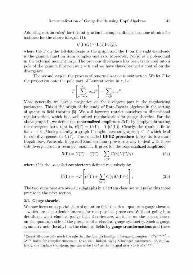
Renormalization of Gauge Fields using Hopf Algebras 141
Adopting certain rules1 for this integration in complex dimensions, one obtains forinstance for the above integral (1):
U(Γ)(z) ∼ Γ(z)Pol(p),
where the Γ on the left-hand-side is the graph and the Γ on the right-hand-sideis the gamma function from complex analysis. Moreover, Pol(p) is a polynomialin the external momentum p. The previous divergence has been translated into apole of the gamma function at z = 0 and we have thus obtained a control on thedivergence.
The second step in the process of renormalization is subtraction. We let T bethe projection onto the pole part of Laurent series in z, i.e.,
T
[ ∞∑n=−∞
anzn
]=∑n<0
anzn.
More generally, we have a projection on the divergent part in the regularizingparameter. This is the origin of the study of Rota-Baxter algebras in the settingof quantum field theories [5]. We will however restrict ourselves to dimensionalregularization, which is a well suited regularization for gauge theories. For theabove graph Γ, we define the renormalized amplitude R(Γ) by simply subtractingthe divergent part, that is, R(Γ) = U(Γ) − T [U(Γ)]. Clearly, the result is finitefor z → 0. More generally, a graph Γ might have subgraphs γ ⊂ Γ which leadto sub-divergences in U(Γ). The so-called BPHZ-procedure (after its inventorsBogoliubov, Parasiuk, Hepp and Zimmermann) provides a way to deal with thosesub-divergences in a recursive manner. It gives for the renormalized amplitude:
R(Γ) = U(Γ) + C(Γ) +∑γ⊂Γ
C(γ)U(Γ/γ) (2a)
where C is the so-called counterterm defined recursively by
C(Γ) = −T
⎡⎣U(Γ) +∑γ⊂Γ
C(γ)U(Γ/γ)
⎤⎦ . (2b)
The two sums here are over all subgraphs in a certain class; we will make this moreprecise in the next section.
2.1. Gauge theories
We now focus on a special class of quantum field theories – quantum gauge theories– which are of particular interest for real physical processes. Without going intodetails on what classical gauge field theories are, we focus on the consequenceson the quantum side of the presence of a classical gauge symmetry. Such a gaugesymmetry acts (locally) on the classical fields by gauge transformations and these
1Essentially, one only needs the rule that the formula familiar in integer dimension∫
dDe−πλk2=
λD/2 holds for complex dimension D as well. Indeed, using Schwinger parameters, or, equiva-
lently, the Laplace transform, one can write 1/k2 as the integral over s > 0 of e−sk2.
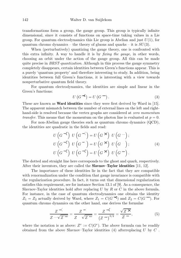
142 Walter D. van Suijlekom
transformations form a group, the gauge group. This group is typically infinitedimensional, since it consists of functions on space-time taking values in a Liegroup. For quantum electrodynamics this Lie group is Abelian and just U(1), forquantum chromo dynamics – the theory of gluons and quarks – it is SU(3).
When (perturbatively) quantizing the gauge theory, one is confronted withthis extra infinity. A way to handle it is by fixing the gauge, in other words,choosing an orbit under the action of the gauge group. All this can be madequite precise in BRST-quantization. Although in this process the gauge symmetrycompletely disappears, certain identities between Green’s functions appear. This isa purely ‘quantum property’ and therefore interesting to study. In addition, beingidentities between full Green’s functions, it is interesting with a view towardsnonperturbative quantum field theory.
For quantum electrodynamics, the identities are simple and linear in theGreen’s functions:
U(G
)= U
(G
). (3)
These are known as Ward identities since they were first derived by Ward in [15].The apparent mismatch between the number of external lines on the left and right-hand-side is resolved because the vertex graphs are considered at zero momentumtransfer. This means that the momentum on the photon line is evaluated at p = 0.
For non-Abelian gauge theories such as quantum chromo dynamics (QCD),the identities are quadratic in the fields and read:
U(G
)U(G
)= U
(G
)U(G
);
U(G
)U(G
)= U
(G
)U(G
);
U(G
)U(G
)= U
(G
)U(G
).
(4)
The dotted and straight line here corresponds to the ghost and quark, respectively.After their inventors, they are called the Slavnov–Taylor identities [11, 12].
The importance of these identities lie in the fact that they are compatiblewith renormalization under the condition that gauge invariance is compatible withthe regularization procedure. In fact, it turns out that dimensional regularizationsatisfies this requirement, see for instance Section 13.1 of [9]. As a consequence, theSlavnov-Taylor identities hold after replacing U by R or C in the above formula.For instance, in the case of quantum electrodynamics one obtains the identityZ1 = Z2 actually derived by Ward, where Z1 = C(G ) and Z2 = C(G ). Forquantum chromo dynamics on the other hand, one derives the formulae
Z
Z√Z
=Z
Z√Z
=Z(
Z)3/2
=
√Z
Z, (5)
where the notation is as above: Zr := C(Gr). The above formula can be readilyobtained from the above Slavnov–Taylor identities (4) afterreplacing U by C .
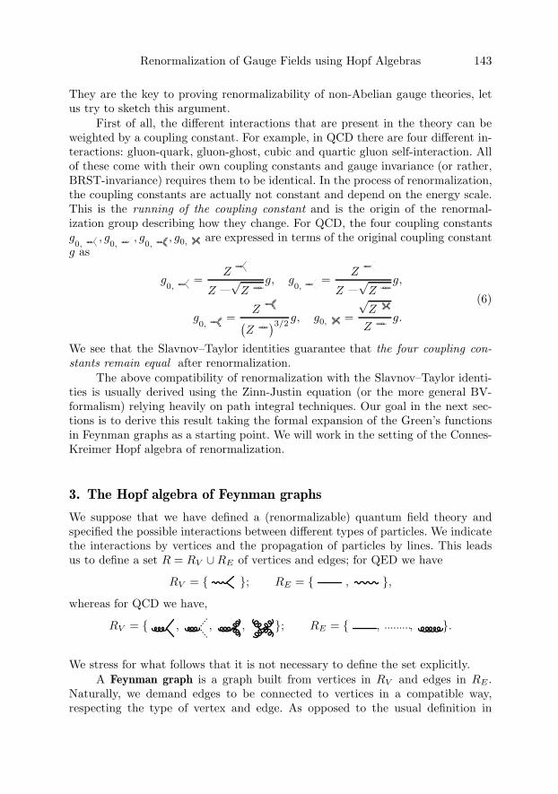
Renormalization of Gauge Fields using Hopf Algebras 143
They are the key to proving renormalizability of non-Abelian gauge theories, letus try to sketch this argument.
First of all, the different interactions that are present in the theory can beweighted by a coupling constant. For example, in QCD there are four different in-teractions: gluon-quark, gluon-ghost, cubic and quartic gluon self-interaction. Allof these come with their own coupling constants and gauge invariance (or rather,BRST-invariance) requires them to be identical. In the process of renormalization,the coupling constants are actually not constant and depend on the energy scale.This is the running of the coupling constant and is the origin of the renormal-ization group describing how they change. For QCD, the four coupling constantsg0,
, g0,
, g0,
, g0, are expressed in terms of the original coupling constantg as
g0,
=Z
Z√Z
g, g0,
=Z
Z√Z
g,
g0,
=Z(
Z)3/2
g, g0, =
√Z
Zg.
(6)
We see that the Slavnov–Taylor identities guarantee that the four coupling con-stants remain equal after renormalization.
The above compatibility of renormalization with the Slavnov–Taylor identi-ties is usually derived using the Zinn-Justin equation (or the more general BV-formalism) relying heavily on path integral techniques. Our goal in the next sec-tions is to derive this result taking the formal expansion of the Green’s functionsin Feynman graphs as a starting point. We will work in the setting of the Connes-Kreimer Hopf algebra of renormalization.
3. The Hopf algebra of Feynman graphs
We suppose that we have defined a (renormalizable) quantum field theory andspecified the possible interactions between different types of particles. We indicatethe interactions by vertices and the propagation of particles by lines. This leadsus to define a set R = RV ∪RE of vertices and edges; for QED we have
RV = { }; RE = { , },whereas for QCD we have,
RV = { , , , }; RE = { , , }.
We stress for what follows that it is not necessary to define the set explicitly.A Feynman graph is a graph built from vertices in RV and edges in RE .
Naturally, we demand edges to be connected to vertices in a compatible way,respecting the type of vertex and edge. As opposed to the usual definition in

144 Walter D. van Suijlekom
graph theory, Feynman graphs have no external vertices, they only have externallines. We assume those lines to carry a labelling.
An automorphism of a Feynman graph is a graph automorphism leaving theexternal lines fixed and respects the types of vertices and edges. This definitionis motivated by the fact that the external lines correspond physically to particlesprepared for some collision experiment – the interior of the graph – and those linesare thus fixed. The order of the group of automorphisms Aut(Γ) of a graph Γ iscalled its symmetry factor and denoted by Sym(Γ). Let us give two examples:
Sym( )
= 2; Sym( )
= 1.
For disconnected graphs, the symmetry factor is given recursively as follows. LetΓ′ be a connected graph; we set
Sym(Γ Γ′) = (n(Γ,Γ′) + 1)Sym(Γ)Sym(Γ′), (7)
with n(Γ,Γ′) the number of connected components of Γ that are isomorphic to Γ′.We define the residue res(Γ) of a graph Γ as the vertex or edge the graph
reduces to after collapsing all its internal vertices and edges to a point. For example,we have:
res
( )= and res
( )= .
Henceforth, we will restrict to graphs with residue in R; these are the relevantgraphs to be considered for the purpose of renormalization.
For later use, we introduce another combinatorial quantity, which is the num-ber of insertion places Γ | γ for the graph γ in Γ. It is defined as the number ofelements in the set of vertices and internal edges of Γ of the form res(γ) ∈ R. Fordisconnected graphs γ = γ1 ∪ · · · ∪ γn, the number Γ | γ counts the number ofn− tuples of disjoint insertion places of the type res(γ1), · · · , res(γn).
We exemplify this quantity by
∣∣∣ = 2 whereas∣∣∣ = 6.
Here, one allows multiple insertions of edge graphs (i.e. a graph with residue inRE) on the same edge; the underlying philosophy is that insertion of an edge graphcreates a new edge.
For the definition of the Hopf algebra of Feynman graphs [3], we restrictto one-particle irreducible (1PI) Feynman graphs. These are graphs that are nottrees and cannot be disconnected by cutting a single internal edge. For example,
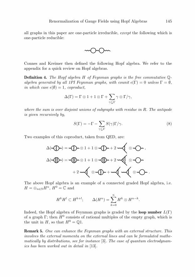
Renormalization of Gauge Fields using Hopf Algebras 145
all graphs in this paper are one-particle irreducible, except the following which isone-particle reducible:
.
Connes and Kreimer then defined the following Hopf algebra. We refer to theappendix for a quick review on Hopf algebras.
Definition 4. The Hopf algebra H of Feynman graphs is the free commutative Q-algebra generated by all 1PI Feynman graphs, with counit ε(Γ) = 0 unless Γ = ∅,in which case ε(∅) = 1, coproduct,
Δ(Γ) = Γ⊗ 1 + 1⊗ Γ +∑γ�Γ
γ ⊗ Γ/γ,
where the sum is over disjoint unions of subgraphs with residue in R. The antipodeis given recursively by,
S(Γ) = −Γ−∑γ�Γ
S(γ)Γ/γ. (8)
Two examples of this coproduct, taken from QED, are:
Δ( ) = ⊗ 1 + 1⊗ + 2 ⊗ ,
Δ( ) = ⊗ 1 + 1⊗ + 2 ⊗
+ 2 ⊗ + ⊗ .
The above Hopf algebra is an example of a connected graded Hopf algebra, i.e.H = ⊕n∈NH
n, H0 = C and
HkH l ⊂ Hk+l; Δ(Hn) =n∑
k=0
Hk ⊗Hn−k.
Indeed, the Hopf algebra of Feynman graphs is graded by the loop number L(Γ)of a graph Γ; then H0 consists of rational multiples of the empty graph, which isthe unit in H , so that H0 = Q1.
Remark 5. One can enhance the Feynman graphs with an external structure. Thisinvolves the external momenta on the external lines and can be formulated mathe-matically by distributions, see for instance [3]. The case of quantum electrodynam-ics has been worked out in detail in [13].

146 Walter D. van Suijlekom
3.1. Renormalization as a Birkhoff decomposition
We now demonstrate how to obtain Equation (2) for the renormalized amplitudeand the counterterm for a graph as a Birkhoff decomposition in the group ofcharacters of H . Let us first recall the definition of a Birkhoff decomposition.
We let l : C → G be a loop with values in an arbitrary complex Lie group G,defined on a smooth simple curve C ⊂ P1(C). Let C± be the two complements ofC in P1(C), with ∞ ∈ C−. A Birkhoff decomposition of l is a factorization of theform
l(z) = l−(z)−1l+(z); (z ∈ C),where l± are (boundary values of) two holomorphic maps on C±, respectively, withvalues in G. This decomposition gives a natural way to extract finite values froma divergent expression. Indeed, although l(z) might not holomorphically extend toC+, l+(z) is clearly finite as z → 0.
C
C+
C− ∞
0
We now look at the group G(K) = HomQ(H,K) of K-valued characters of aconnected graded commutative Hopf algebra H , where K is the field of convergentLaurent series in z.2 The product, inverse and unit in the group G(K) are definedby the respective equations:
φ ∗ ψ(X) = 〈φ ⊗ ψ,Δ(X)〉,φ−1(X) = φ(S(X)),
e(X) = ε(X),
for φ, ψ ∈ G(K). We claim that a map φ ∈ G(K) is in one-to-one correspon-dence with loops l on an infinitesimal circle around z = 0 and values in G(Q) =HomQ(H,Q). Indeed, the correspondence is given by
φ(X)(z) = l(z)(X),
2In the language of algebraic geometry, there is an affine group scheme G represented by H inthe category of commutative algebras. In other words, G = HomQ(H, . ) and G(K) are the
K-points of the group scheme.
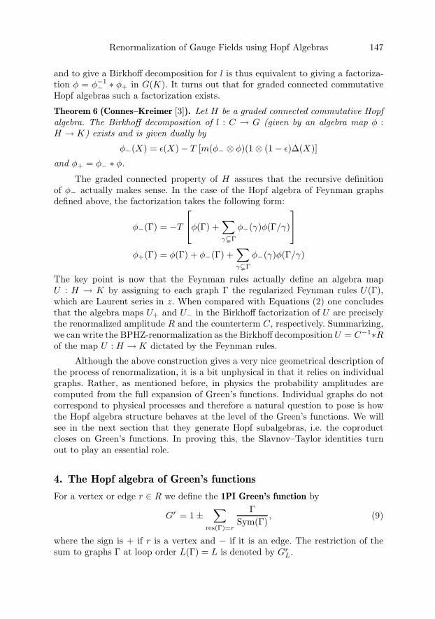
Renormalization of Gauge Fields using Hopf Algebras 147
and to give a Birkhoff decomposition for l is thus equivalent to giving a factoriza-tion φ = φ−1
− ∗ φ+ in G(K). It turns out that for graded connected commutativeHopf algebras such a factorization exists.
Theorem 6 (Connes–Kreimer [3]). Let H be a graded connected commutative Hopfalgebra. The Birkhoff decomposition of l : C → G (given by an algebra map φ :H → K) exists and is given dually by
φ−(X) = ε(X)− T [m(φ− ⊗ φ)(1 ⊗ (1 − ε)Δ(X)]
and φ+ = φ− ∗ φ.
The graded connected property of H assures that the recursive definitionof φ− actually makes sense. In the case of the Hopf algebra of Feynman graphsdefined above, the factorization takes the following form:
φ−(Γ) = −T
⎡⎣φ(Γ) +∑γ�Γ
φ−(γ)φ(Γ/γ)
⎤⎦φ+(Γ) = φ(Γ) + φ−(Γ) +
∑γ�Γ
φ−(γ)φ(Γ/γ)
The key point is now that the Feynman rules actually define an algebra mapU : H → K by assigning to each graph Γ the regularized Feynman rules U(Γ),which are Laurent series in z. When compared with Equations (2) one concludesthat the algebra maps U+ and U− in the Birkhoff factorization of U are preciselythe renormalized amplitude R and the counterterm C, respectively. Summarizing,we can write the BPHZ-renormalization as the Birkhoff decomposition U = C−1∗Rof the map U : H → K dictated by the Feynman rules.
Although the above construction gives a very nice geometrical description ofthe process of renormalization, it is a bit unphysical in that it relies on individualgraphs. Rather, as mentioned before, in physics the probability amplitudes arecomputed from the full expansion of Green’s functions. Individual graphs do notcorrespond to physical processes and therefore a natural question to pose is howthe Hopf algebra structure behaves at the level of the Green’s functions. We willsee in the next section that they generate Hopf subalgebras, i.e. the coproductcloses on Green’s functions. In proving this, the Slavnov–Taylor identities turnout to play an essential role.
4. The Hopf algebra of Green’s functions
For a vertex or edge r ∈ R we define the 1PI Green’s function by
Gr = 1±∑
res(Γ)=r
ΓSym(Γ)
, (9)
where the sign is + if r is a vertex and − if it is an edge. The restriction of thesum to graphs Γ at loop order L(Γ) = L is denoted by Gr
L.

148 Walter D. van Suijlekom
Proposition 7 ([14]). The coproduct takes the following form on the 1PI Green’sfunctions:
Δ(Gr) =∑
γ
∑res(Γ)=r
Γ | γSym(γ)Sym(Γ)
γ ⊗ Γ,
with the sum over γ over all disjoint unions of 1PI graphs.
The sketch of the proof is as follows. First, one writes the coproduct Δ as asum of maps Δγ where these maps only detects subgraphs isomorphic to γ. Onethen proves the above formula for Δγ with γ a 1PI graph using simply the orbit-stabilizer theorem for the automorphism group of graphs. Finally, writing Δγγ′ interms of Δγ and Δγ′ one proceeds by induction to derive the above expression.
One observes that the coproduct does not seem to close on Green’s functionsdue to the appearance of the combinatorial factor Γ | γ. Let us try to elucidatethis and compute these factors explicitly.
Let mΓ,r be the number of vertices/internal edges of type r appearing in Γ,for r ∈ R. Moreover, let nγ,r be the number of connected components of γ withresidue r. Since insertion of a vertex graph (i.e. with residue in RV ) on a vertex vin Γ prevents a subsequent insertion at v of a vertex graph with the same residue,whereas insertion of an edge graph (i.e. with residue in RE) creates two new edgesand hence two insertion places for a subsequent edge graph, we find the followingexpression,
Γ | γ =∏
v∈RV
nγ,v!(mΓ,v
nγ,v
) ∏e∈RE
nγ,e!(mΓ,e + nγ,e − 1
nγ,e
).
Indeed, the binomial coefficients arise for each vertex v since we are choosing nγ,v
out of mΓ,v whereas for an edge e we choose nγ,e out of mΓ,e with repetition.We claim that this counting enhances our formula to the following
Δ(Gr) =∑
res(Γ)=r
∏v∈RV
(Gv)mΓ,v∏
e∈RE
(Ge)−mΓ,e ⊗ ΓSym(Γ)
. (10)
Before proving this, we explain the meaning of the inverse of Green’s functionsin our Hopf algebra. Since any Green’s function starts with the identity, we cansurely write its inverse formally as a geometric series. Recall that the Hopf algebrais graded by loop number. Hence, the inverse of a Green’s function at a fixedloop order is in fact well-defined; it is given by restricting the above formal seriesexpansion to this loop order. In the following, also rational powers of Green’sfunctions will appear; they will be understood in like manner.
Proof of Eq. (10). Let us simplify a little and consider a scalar field theory withjust one type of vertex and edge, i.e. R = { , }. We consider the sum∑
γ
Γ | γSym(γ)
γ =∑γv
nγ,v!Sym(γv)
(mΓ,v
nγ,v
)γv
∑γe
nγ,e!Sym(γe)
(mΓ,e + nγ,v − 1
nγ,v
)γe,

Renormalization of Gauge Fields using Hopf Algebras 149
naturally split into a sum over vertex and edge graphs. We have also inserted theabove combinatorial expression for the number of insertion places. Next, we writeγv = γ′
vγ′′v and try factorize the sum over γv into a sum over γ′
v (connected) andγ′′
v . Some care should be taken here regarding the combinatorial factors but let usignore them for the moment. In fact, if we fix the number of connected componentsh0(γv) of γv in the sum to be nV we can write
∑h0(γv)=nV
nV !γv
Sym(γv)=
∑h0(γv)=nV
⎛⎜⎜⎜⎝ ∑γ′
v,γ′′v
γ′vγ′′
v �γv
n(γ′′v , γ
′v) + 1
nV
⎞⎟⎟⎟⎠nV !γv
Sym(γv),
with γ′v a connected graph. Here, we have simply inserted 1,∑
γ′v,γ′′
v
γ′vγ′′
v �γv
n(γ′′v , γ
′v) + 1
nV=∑γ′
v
n(γv, γ′v)
nV= 1,
which follows directly from the definition of n(γv, γ′v) as the number of connected
components of γv isomorphic to γ′v. Now, by definition Sym(γ′
vγ′′v ) = (n(γ′′
v , γ′v) +
1)Sym(γ′v)Sym(γ′′
v ) for a connected graph γ′v so that we obtain for the above sum∑
γ′v
γ′v
Sym(γ′v)
∑h0(γ′′
v )=nV −1
(nV − 1)!γ′′
v
Sym(γ′′v )
= · · · = (Gv − 1)nV ,
by applying the same argument nV times. Recall also the definition of the Green’sfunction Gv from Eq. (9). A similar argument applies to the edge graphs, leadingto a contribution (1 − Ge)nE , with nE the number of connected components ofγe. When summing over nV and nE, taking also into account the combinatorialfactors, we obtain:∞∑
nV =0
(mΓ,v
nV
)(Gv − 1)nV
∞∑nE=0
(mΓ,e + nE − 1
nE
)(1−Ge)nE = (Gv)mΓ,v (Ge)−mΓ,e .
The extension to the general setting where the set R contains different types ofvertices and edges is straightforward. �
An additional counting of the number of edges and numbers of vertices in Γgives the following relations:
2mΓ,e + Ne(res(Γ)) =∑
v∈RV
Ne(v)mΓ,v
where Ne(r) is the number of lines (of type e) attached to r ∈ R. For instanceNe( ) equals 2 if e is an electron line and 1 if e is a photon line. One checks theabove equality by noting that the left-hand-side counts the number of internal halflines plus the external lines which are connected to the vertices that appear at theright-hand-side, taken into account their valence.

150 Walter D. van Suijlekom
With this formula, we can write Eq. (10) as
Δ(Gr) =∏e
(Ge)Ne(r)/2∑
res(Γ)=r
∏v
(Gv∏
e (Ge)Ne(v)/2
)mΓ,v
⊗ ΓSym(Γ)
. (11)
This is still not completely satisfactory since it involves the number of verticesin Γ which prevents us from separating the summation of Γ from the other terms.We introduce the following notation for the fraction of Green’s functions above:
Xv =
(Gv∏
e (Ge)Ne(v)/2
)1/(N(v)−2)
(12)
with N(v) the total number of edges attached to v. Before we state our maintheorem, let us motivate the definition of these elements in the case of QCD.
Example 8. In QCD, there are four vertices and the corresponding elements Xv
are given by,
X =G
G√G
, X =G
G√G
,
X =G(
G)3/2
, X =
√G
G.
The combinations of the Green’s functions are identical to those appearing in for-mulas (5). Indeed, as we will see in a moment, setting them equal in H is com-patible with the coproduct.
Although motivated by the study of the Slavnov–Taylor identities in non-Abelian gauge theories, the following result holds in complete generality.
Theorem 9. The ideal I = 〈Xv −Xv′〉v′∈RV is a Hopf ideal, i.e.
Δ(I) ⊂ I ⊗H + H ⊗ I, ε(I) = 0, S(I) ⊂ I.
Proof. Let us write the above Eq. (11) in terms of the Xv’s:
Δ(Gr) =∏e
(Ge)12Ne(r)
∑res(Γ)=r
∏v′
(Xv′)(N(v′)−2)mΓ,v′ ⊗ ΓSym(Γ)
.
In this expression, Xv′ appears with a certain power, say s, and we can replace(Xv′)s by (Xv)s as long as we add the term (Xv′)s − (Xv)s. This latter term canbe factorized as Xv′ − Xv times a certain polynomial in Xv and Xv′ and thuscorresponds to an element in I. As a result, we can replace all Xv′ ’s by Xv forsome fixed v modulo addition of terms in I ⊗H .
The second step uses the following equality between vertices and edges:∑v′∈RV
(N(v′)− 2)mΓ,v′ = 2L + N(r) − 2 (13)
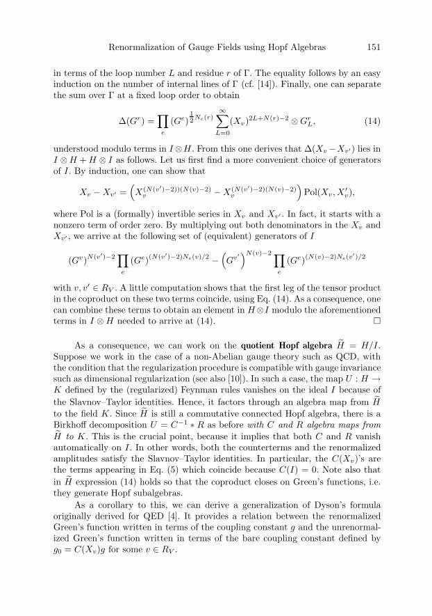
Renormalization of Gauge Fields using Hopf Algebras 151
in terms of the loop number L and residue r of Γ. The equality follows by an easyinduction on the number of internal lines of Γ (cf. [14]). Finally, one can separatethe sum over Γ at a fixed loop order to obtain
Δ(Gr) =∏e
(Ge)12Ne(r)
∞∑L=0
(Xv)2L+N(r)−2 ⊗GrL, (14)
understood modulo terms in I⊗H . From this one derives that Δ(Xv−Xv′) lies inI ⊗H + H ⊗ I as follows. Let us first find a more convenient choice of generatorsof I. By induction, one can show that
Xv −Xv′ =(X(N(v′)−2))(N(v)−2)
v −X(N(v′)−2)(N(v)−2)v
)Pol(Xv, X
′v),
where Pol is a (formally) invertible series in Xv and Xv′ . In fact, it starts with anonzero term of order zero. By multiplying out both denominators in the Xv andXv′ , we arrive at the following set of (equivalent) generators of I
(Gv)N(v′)−2∏e
(Ge)(N(v′)−2)Ne(v)/2 −(Gv′)N(v)−2 ∏
e
(Ge)(N(v)−2)Ne(v′)/2
with v, v′ ∈ RV . A little computation shows that the first leg of the tensor productin the coproduct on these two terms coincide, using Eq. (14). As a consequence, onecan combine these terms to obtain an element in H⊗I modulo the aforementionedterms in I ⊗H needed to arrive at (14). �
As a consequence, we can work on the quotient Hopf algebra H = H/I.Suppose we work in the case of a non-Abelian gauge theory such as QCD, withthe condition that the regularization procedure is compatible with gauge invariancesuch as dimensional regularization (see also [10]). In such a case, the map U : H →K defined by the (regularized) Feynman rules vanishes on the ideal I because ofthe Slavnov–Taylor identities. Hence, it factors through an algebra map from H
to the field K. Since H is still a commutative connected Hopf algebra, there is aBirkhoff decomposition U = C−1 ∗ R as before with C and R algebra maps fromH to K. This is the crucial point, because it implies that both C and R vanishautomatically on I. In other words, both the counterterms and the renormalizedamplitudes satisfy the Slavnov–Taylor identities. In particular, the C(Xv)’s arethe terms appearing in Eq. (5) which coincide because C(I) = 0. Note also thatin H expression (14) holds so that the coproduct closes on Green’s functions, i.e.they generate Hopf subalgebras.
As a corollary to this, we can derive a generalization of Dyson’s formulaoriginally derived for QED [4]. It provides a relation between the renormalizedGreen’s function written in terms of the coupling constant g and the unrenormal-ized Green’s function written in terms of the bare coupling constant defined byg0 = C(Xv)g for some v ∈ RV .
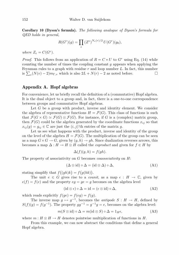
152 Walter D. van Suijlekom
Corollary 10 (Dyson’s formula). The following analogue of Dyson’s formula forQED holds in general,
R(Gr)(g) =∏e
(Ze)Ne(r)/2U(Gr)(g0),
where Ze = C(Ge).
Proof. This follows from an application of R = C ∗ U to Gr using Eq. (14) whilecounting the number of times the coupling constant g appears when applying theFeynman rules to a graph with residue r and loop number L. In fact, this numberis∑
v(N(v)− 2)mΓ,v which is also 2L + N(r) − 2 as noted before. �
Appendix A. Hopf algebras
For convenience, let us briefly recall the definition of a (commutative) Hopf algebra.It is the dual object to a group and, in fact, there is a one-to-one correspondencebetween groups and commutative Hopf algebras.
Let G be a group with product, inverse and identity element. We considerthe algebra of representative functions H = F(G). This class of functions is suchthat F(G × G) � F(G) ⊗ F(G). For instance, if G is a (complex) matrix group,then F(G) could be the algebra generated by the coordinate functions xij so thatxij(g) = gij ∈ C are just the (i, j)’th entries of the matrix g.
Let us see what happens with the product, inverse and identity of the groupon the level of the algebra H = F(G). The multiplication of the group can be seenas a map G×G→ G, given by (g, h) → gh. Since dualization reverses arrows, thisbecomes a map Δ : H → H ⊗H called the coproduct and given for f ∈ H by
Δ(f)(g, h) = f(gh).
The property of associativity on G becomes coassociativity on H :
(Δ⊗ id) ◦Δ = (id⊗Δ) ◦Δ, (A1)
stating simplify that f((gh)k
)= f
(g(hk)
).
The unit e ∈ G gives rise to a counit, as a map ε : H → C, given byε(f) = f(e) and the property eg = ge = g becomes on the algebra level
(id⊗ ε) ◦Δ = id = (ε⊗ id) ◦Δ, (A2)
which reads explicitly f(ge) = f(eg) = f(g).The inverse map g �→ g−1, becomes the antipode S : H → H , defined by
S(f)(g) = f(g−1). The property gg−1 = g−1g = e, becomes on the algebra level:
m(S ⊗ id) ◦Δ = m(id⊗ S) ◦Δ = 1Hε, (A3)
where m : H ⊗H → H denotes pointwise multiplication of functions in H .From this example, we can now abstract the conditions that define a general
Hopf algebra.
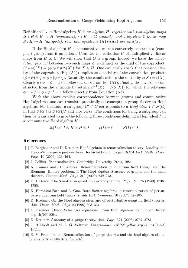
Renormalization of Gauge Fields using Hopf Algebras 153
Definition 11. A Hopf algebra H is an algebra H, together with two algebra mapsΔ : H ⊗ H → H (coproduct), ε : H → C (counit), and a bijective C-linear mapS : H → H (antipode), such that equations (A1)–(A3) are satisfied.
If the Hopf algebra H is commutative, we can conversely construct a (com-plex) group from it as follows. Consider the collection G of multiplicative linearmaps from H to C. We will show that G is a group. Indeed, we have the convo-lution product between two such maps φ, ψ defined as the dual of the coproduct:(φ ∗ ψ)(X) = (φ ⊗ ψ)(Δ(X)) for X ∈ H . One can easily check that coassociativ-ity of the coproduct (Eq. (A1)) implies associativity of the convolution product:(φ ∗ ψ) ∗ χ = φ ∗ (ψ ∗ χ). Naturally, the counit defines the unit e by e(X) = ε(X).Clearly e ∗φ = φ = φ ∗ e follows at once from Eq. (A2). Finally, the inverse is con-structed from the antipode by setting φ−1(X) = φ(S(X)) for which the relationsφ−1 ∗ φ = φ ∗ φ−1 = e follow directly from Equation (A3).
With the above explicit correspondence between groups and commutativeHopf algebras, one can translate practically all concepts in group theory to Hopfalgebras. For instance, a subgroup G′ ⊂ G corresponds to a Hopf ideal I ⊂ F(G)in that F(G′) � F(G)/I and vice versa. The conditions for being a subgroup canthen be translated to give the following three conditions defining a Hopf ideal I ina commutative Hopf algebra H
Δ(I) ⊂ I ⊗H + H ⊗ I, ε(I) = 0, S(I) ⊂ I.
References
[1] C. Bergbauer and D. Kreimer. Hopf algebras in renormalization theory: Locality andDyson-Schwinger equations from Hochschild cohomology. IRMA Lect. Math. Theor.Phys. 10 (2006) 133–164.
[2] J. Collins. Renormalization. Cambridge University Press, 1984.
[3] A. Connes and D. Kreimer. Renormalization in quantum field theory and theRiemann- Hilbert problem. I: The Hopf algebra structure of graphs and the maintheorem. Comm. Math. Phys. 210 (2000) 249–273.
[4] F. J. Dyson. The S matrix in quantum electrodynamics. Phys. Rev. 75 (1949) 1736–1755.
[5] K. Ebrahimi-Fard and L. Guo. Rota-Baxter algebras in renormalization of pertur-bative quantum field theory. Fields Inst. Commun. 50 (2007) 47–105.
[6] D. Kreimer. On the Hopf algebra structure of perturbative quantum field theories.Adv. Theor. Math. Phys. 2 (1998) 303–334.
[7] D. Kreimer. Dyson–Schwinger equations: From Hopf algebras to number theory.hep-th/0609004.
[8] D. Kreimer. Anatomy of a gauge theory. Ann. Phys. 321 (2006) 2757–2781.
[9] G. ’t Hooft and M. J. G. Veltman. Diagrammar. CERN yellow report. 73 (1973)1–114.
[10] D. V. Prokhorenko. Renormalization of gauge theories and the hopf algebra of dia-grams. arXiv:0705.3906 [hep-th].

154 Walter D. van Suijlekom
[11] A. A. Slavnov. Ward identities in gauge theories. Theor. Math. Phys. 10 (1972)99–107.
[12] J. C. Taylor. Ward identities and charge renormalization of the yang-mills field. Nucl.Phys. B33 (1971) 436–444.
[13] W. D. van Suijlekom. The Hopf algebra of Feynman graphs in QED. Lett. Math.Phys. 77 (2006) 265–281.
[14] W. D. van Suijlekom. Renormalization of gauge fields: A Hopf algebra approach.Commun. Math. Phys. 276 (2007) 773–798.
[15] J. C. Ward. An identity in quantum electrodynamics. Phys. Rev. 78 (1950) 182.
Walter D. van SuijlekomInstitute for Mathematics, Astrophysics and Particle PhysicsFaculty of Science, Radboud Universiteit NijmegenToernooiveld 1NL–6525 ED Nijmegene-mail: [email protected]
Quantum Field TheoryB. Fauser, J. Tolksdorf and E. Zeidler, Eds., 155–162c© 2009 Birkhauser Verlag Basel/Switzerland
Not so Non-Renormalizable Gravity
Dirk Kreimer
Abstract. We review recent ideas [1] how gravity might turn out to be arenormalizable theory after all.
Mathematics Subject Classification (2000). Primary 81T15; Secondary 81T13;83C47.
Keywords. gravitation, renormalization, Feynman rules, Dyson-Schwingerequations, gauge theory, perturbative methods.
1. Introduction
Renormalizable perturbative quantum field theories are embarrassingly success-ful in describing observed physics. Whilst their mathematical structure is stilla challenge albeit an entertaining one, they are testimony to some of the finestachievements in our understanding of nature. The physical laws as far as theyare insensitive to the surrounding geometry seems completely described by suchtheories. Alas, if we incorporate gravity, and want to quantize it, we seem at aloss.
In this talk, we report on some recent work [1] which might give hope. Ourmain purpose is to review the basic idea and to put it into context.
As in [1], we will proceed by a comparison of the structure of a renormalizabletheory, quantum electrodynamics in four dimensions, and gravity.
It is the role of the Hochschild cohomology [2] in those two different situations,which leads to surprising new insights. We will discuss them at an elementary levelfor the situation of pure gravity. We also allow, in the spirit of the workshop forthe freedom to muse about conceptual consequences at the end.
Talk given at the “Max Planck Institute for Mathematics in the Natural Sciences”, Leipzig. Worksupported in parts by grant NSF-DMS/0603781. Author supported by CNRS.
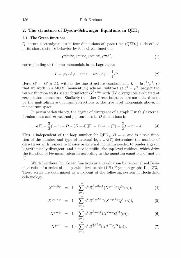
156 Dirk Kreimer
2. The structure of Dyson–Schwinger Equations in QED4
2.1. The Green functions
Quantum electrodynamics in four dimensions of space-time (QED4) is describedin its short-distance behavior by four Green functions
Gψγ·∂ψ, Gmψψ , Gψγ·Aψ, G14 F 2
, (1)
corresponding to the four monomials in its Lagrangian
L = ψγ · ∂ψ − ψmψ − ψγ · Aψ − 14F 2. (2)
Here, Gi = Gi(α,L), with α the fine structure constant and L = ln q2/μ2, sothat we work in a MOM (momentum) scheme, subtract at q2 = μ2, project thevertex function to its scalar formfactor Gψγ·∂ψ with UV divergences evaluated atzero photon momentum. Similarly the other Green functions are normalized as tobe the multiplicative quantum corrections to the tree level monomials above, inmomentum space.
In perturbation theory, the degree of divergence of a graph Γ with f externalfermion lines and m external photon lines in D dimensions is
ωD(Γ) =32f + m−D − (D − 4)(|Γ| − 1) ⇒ ω4(Γ) =
32f + m− 4. (3)
This is independent of the loop number for QED4, D = 4, and is a sole func-tion of the number and type of external legs. ωD(Γ) determines the number ofderivatives with respect to masses or external momenta needed to render a graphlogarithmically divergent, and hence identifies the top-level residues, which drivethe iteration of Feynman integrals according to the quantum equations of motion[3].
We define these four Green functions as an evaluation by renormalized Feyn-man rules of a series of one-particle irreducible (1PI) Feynman graphs Γ ∈ FGi.These series are determined as a fixpoint of the following system in Hochschildcohomology.
X ψγ·∂ψ = 1−∞∑
k=1
αkBψγ·∂ψ,k+ (X ψγ·∂ψQ2k(α)), (4)
X ψγ·Aψ = 1 +∞∑
k=1
αkBψγ·Aψ,k+ (X ψγ·AψQ2k(α)), (5)
X ψmψ = 1−∞∑
k=1
αkBψmψ,k+ (X ψmψQ2k(α)), (6)
X14 F 2
= 1−∞∑
k=1
αkB14 F 2,k+ (X
14 F 2
Q2k(α)). (7)

Not so Non-Renormalizable Gravity 157
Here,
Bi,k+ =
∑|γ|=k,Δ′(γ)=0,γ∈FGi
Bγ+, ∀i ∈ RQED, (8)
is a sum over all Hopf algebra primitive graphs with given loop number k andcontributing to superficially divergent amplitude i, and
Bγ+(X) =
∑Γ∈<Γ>
bij(γ,X,Γ)|X |∨
1maxf(Γ)
1(γ|X)
Γ, (9)
where maxf(Γ) is the number of maximal forests of Γ, |X |γ is the number of distinctgraphs obtainable by permuting edges of X , bij(γ,X,Γ) is the number of bijectionsof external edges of X with an insertion place in γ such that the result is Γ, andfinally (γ|X) is the number of insertion places for X in γ [4], and
RQED = {ψγ · ∂ψ, ψγ ·Aψ,mψψ,14F 2}. (10)
Also, we let
Q =X ψγ·Aψ
X ψγ·∂ψ√X
14 F 2
. (11)
The resulting maps Bi,K+ are Hochschild closed
bBi,K+ = 0 (12)
in the sense of [5]. We have in fact
Δ(Bγ+(X)) =
∑Γ
nΓ,X,γΓ (13)
where nΓ,X,γ can be determined from (9,12).Furthermore, one can choose a basis of primitives γ [3] such that their Mellin
transforms Mγ(ρ) have the form
Mγ(ρ) =∫
ιγ(ki; q)|q2=μ2
|γ|∏s=1
[k2s/μ
2]−ρ/|γ|d4ki
(2π)4for 1 > '(ρ) > 0, (14)
where the integrand ιγ is a function of internal momenta ki and an external mo-mentum q, subtracted at q2 = μ2.
The Dyson Schwinger equations then take the form
GiR(α,L) = 1± lim
ρ→0
⎡⎣∑k
αk∑|γ|=k
Gir(α, ∂ρ)Q(α, ∂ρ)Mγ(ρ)
[(q2
μ2
)−ρ
− 1
]⎤⎦(15)
where
ΦR(X i) = GiR(α,L), (16)
and
ΦR(Q) = Q(α,L), (17)
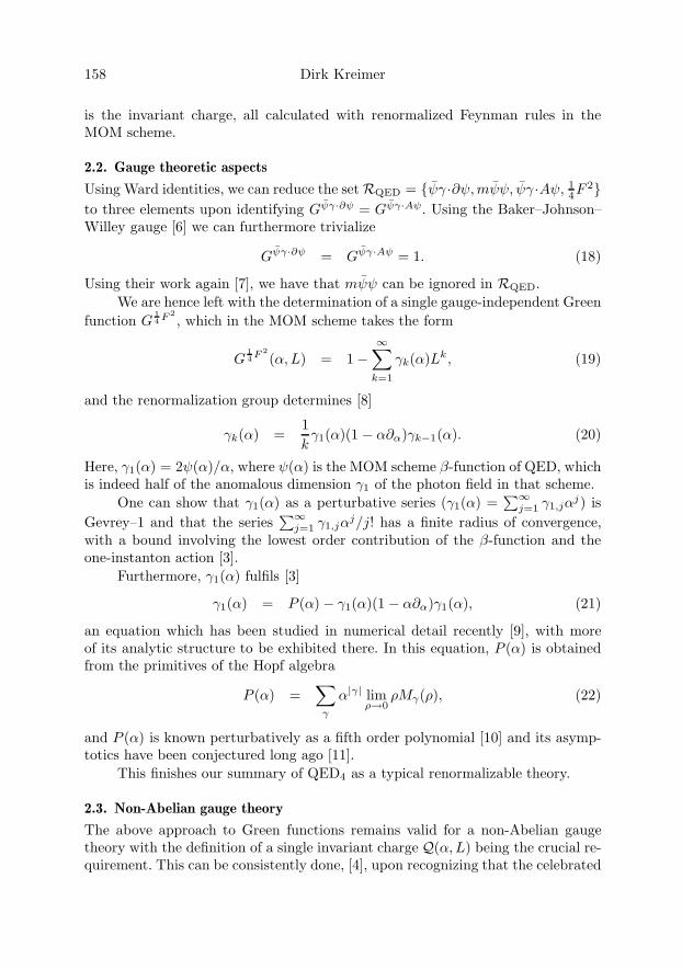
158 Dirk Kreimer
is the invariant charge, all calculated with renormalized Feynman rules in theMOM scheme.
2.2. Gauge theoretic aspects
Using Ward identities, we can reduce the setRQED = {ψγ ·∂ψ,mψψ, ψγ ·Aψ, 14F
2}to three elements upon identifying Gψγ·∂ψ = Gψγ·Aψ. Using the Baker–Johnson–Willey gauge [6] we can furthermore trivialize
Gψγ·∂ψ = Gψγ·Aψ = 1. (18)
Using their work again [7], we have that mψψ can be ignored in RQED.We are hence left with the determination of a single gauge-independent Green
function G14 F 2
, which in the MOM scheme takes the form
G14 F 2
(α,L) = 1−∞∑
k=1
γk(α)Lk, (19)
and the renormalization group determines [8]
γk(α) =1kγ1(α)(1 − α∂α)γk−1(α). (20)
Here, γ1(α) = 2ψ(α)/α, where ψ(α) is the MOM scheme β-function of QED, whichis indeed half of the anomalous dimension γ1 of the photon field in that scheme.
One can show that γ1(α) as a perturbative series (γ1(α) =∑∞
j=1 γ1,jαj) is
Gevrey–1 and that the series∑∞
j=1 γ1,jαj/j! has a finite radius of convergence,
with a bound involving the lowest order contribution of the β-function and theone-instanton action [3].
Furthermore, γ1(α) fulfils [3]
γ1(α) = P (α)− γ1(α)(1 − α∂α)γ1(α), (21)
an equation which has been studied in numerical detail recently [9], with moreof its analytic structure to be exhibited there. In this equation, P (α) is obtainedfrom the primitives of the Hopf algebra
P (α) =∑
γ
α|γ| limρ→0
ρMγ(ρ), (22)
and P (α) is known perturbatively as a fifth order polynomial [10] and its asymp-totics have been conjectured long ago [11].
This finishes our summary of QED4 as a typical renormalizable theory.
2.3. Non-Abelian gauge theory
The above approach to Green functions remains valid for a non-Abelian gaugetheory with the definition of a single invariant charge Q(α,L) being the crucial re-quirement. This can be consistently done, [4], upon recognizing that the celebrated

Not so Non-Renormalizable Gravity 159
Slavnov–Taylor identities for the couplings fulfil
SφR(X ψγ·Aψ)
SφR(X ψγ·∂ψ)
=Sφ
R(XAA∂A)
SφR(X∂A∂A)
=Sφ
R(XAAAA)
SφR(XAA∂A)
=Sφ
R(X φA·∂φ)
SφR(X φ�φ)
(23)
for the set of amplitudes
RQCD = {DADA, ψγ · ∂ψ, φ�φ,AADA,AAAA, φA · ∂φ, ψγ · Aψ}, (24)
needing renormalization in QCD.This allows to define a Hochschild cohomology on the sum of graphs at a given
loop order, and hence to obtain multiplicative renormalization in this languagefrom the resulting coideals in the Hopf algebra [4, 12].1
Note that the structure of the sub-Hopf algebras underlying this approach[5, 8] implies that the elements X i(α) close under the coproduct. A general clas-sification of related sub-Hopf algebras has been recently obtained by Loic Foissy[13]. He considers only the case that the lowest order Hochschild cocycle is presentin the combinatorial Dyson–Schwinger equations, but his study is rather completewhen augmented by the results of [2].
3. Gravity
We consider pure gravity understood as a theory based on a graviton propagatorand n-graviton couplings as vertices. A fuller discussion incorporating ghosts andmatter fields is referred to future work.
3.1. Summary of some results obtained for quantum gravity
We summarize here some results published in [1].
Corollary 1. Let |Γ| = k. Then ω(Γ) = −2(|Γ|+ 1).
This is a significant change from the behavior of a renormalizable theory: inthe renormalizable case, each graph contributing to the same amplitude i has thesame powercounting degree regardless of the loop number. Here, we have the dualsituation: the loop number determines the powercounting degree, regardless of theamplitude.
Theorem 2. The set dω(Γ) contains no primitive element beyond one loop.
The set dω(Γ) is determined as a set of dotted graphs, with dots representingω(Γ) derivatives with respect to masses or external momenta such that the corre-sponding integrand ιΓ is overall log-divergent. Whilst in a renormalizable theory,we find for each amplitude in the finite set R primitives at each loop order indω(Γ), here we have an infinite set R, but only one primitive in it.
1Eds. note: See also W. van Suijlekom’s contribution in this book.
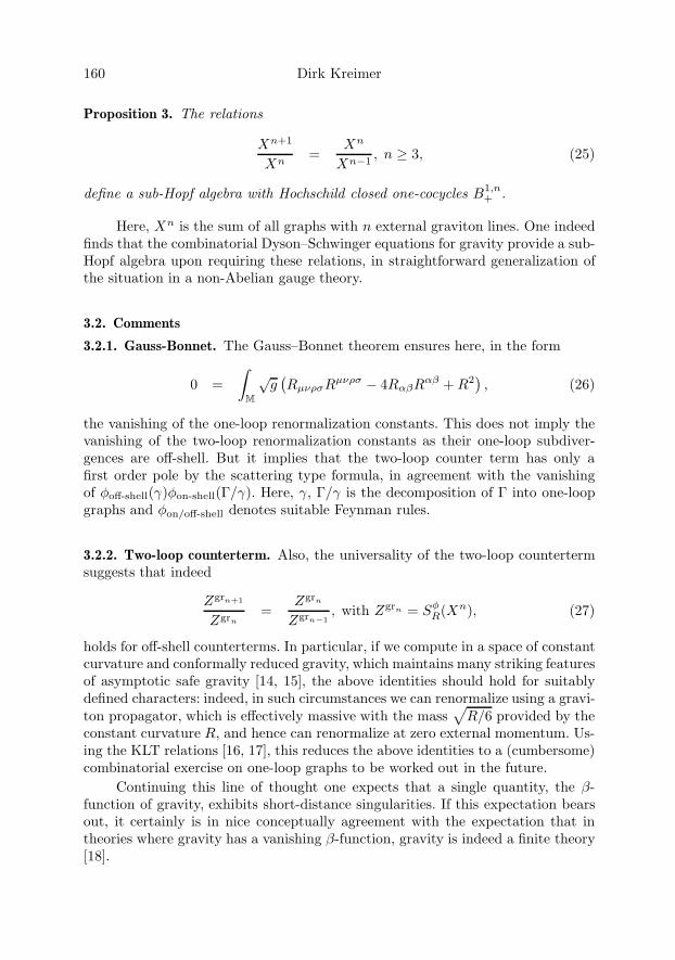
160 Dirk Kreimer
Proposition 3. The relations
Xn+1
Xn=
Xn
Xn−1, n ≥ 3, (25)
define a sub-Hopf algebra with Hochschild closed one-cocycles B1,n+ .
Here, Xn is the sum of all graphs with n external graviton lines. One indeedfinds that the combinatorial Dyson–Schwinger equations for gravity provide a sub-Hopf algebra upon requiring these relations, in straightforward generalization ofthe situation in a non-Abelian gauge theory.
3.2. Comments
3.2.1. Gauss-Bonnet. The Gauss–Bonnet theorem ensures here, in the form
0 =∫
M
√g(RμνρσR
μνρσ − 4RαβRαβ + R2
), (26)
the vanishing of the one-loop renormalization constants. This does not imply thevanishing of the two-loop renormalization constants as their one-loop subdiver-gences are off-shell. But it implies that the two-loop counter term has only afirst order pole by the scattering type formula, in agreement with the vanishingof φoff-shell(γ)φon-shell(Γ/γ). Here, γ, Γ/γ is the decomposition of Γ into one-loopgraphs and φon/off-shell denotes suitable Feynman rules.
3.2.2. Two-loop counterterm. Also, the universality of the two-loop countertermsuggests that indeed
Zgrn+1
Zgrn=
Zgrn
Zgrn−1, with Zgrn = Sφ
R(Xn), (27)
holds for off-shell counterterms. In particular, if we compute in a space of constantcurvature and conformally reduced gravity, which maintains many striking featuresof asymptotic safe gravity [14, 15], the above identities should hold for suitablydefined characters: indeed, in such circumstances we can renormalize using a gravi-ton propagator, which is effectively massive with the mass
√R/6 provided by the
constant curvature R, and hence can renormalize at zero external momentum. Us-ing the KLT relations [16, 17], this reduces the above identities to a (cumbersome)combinatorial exercise on one-loop graphs to be worked out in the future.
Continuing this line of thought one expects that a single quantity, the β-function of gravity, exhibits short-distance singularities. If this expectation bearsout, it certainly is in nice conceptually agreement with the expectation that intheories where gravity has a vanishing β-function, gravity is indeed a finite theory[18].
Not so Non-Renormalizable Gravity 161
3.2.3. Other instances of gravity powercounting. The appearance of Feynmanrules such that the powercounting of vertex amplitudes in RV cancels the pow-ercounting of propagator amplitudes in RE, R = RV ∪ RE, is not restricted togravity. It indeed appears for example also in the field theoretic description of bulkmaterials like glass, which were recently described at tree-level as a field theory[19], and whose renormalization will have powercounting properties similar to thepresent discussion.
Acknowledgements
It is a pleasure to thank Bertfried Fauser, Jurgen Tolksdorf and Eberhard Zeidlerfor inviting me to this workshop.
References
[1] D. Kreimer, A remark on quantum gravity, Annals Phys. 323 (2008) 49[arXiv:0705.3897 [hep-th]].
[2] C. Bergbauer and D. Kreimer, Hopf algebras in renormalization theory: Locality andDyson-Schwinger equations from Hochschild cohomology, IRMA Lect. Math. Theor.Phys. 10 (2006) 133 [arXiv:hep-th/0506190].
[3] D. Kreimer and K. Yeats, An etude in non-linear Dyson-Schwinger equations, Nucl.Phys. Proc. Suppl. 160 (2006) 116 [arXiv:hep-th/0605096].
[4] D. Kreimer, Anatomy of a gauge theory, Annals Phys. 321 (2006) 2757 [arXiv:hep-th/0509135].
[5] D. Kreimer, Dyson–Schwinger Equations: From Hopf algebras to Number Theory, inUniversality and Renormalization, I. Binder, D. Kreimer, eds., Fields Inst Comm. 50(2007) 225, AMS.
[6] K. Johnson, M. Baker and R. Willey, Selfenergy Of The Electron, Phys. Rev. 136(1964) B1111.
[7] M. Baker and K. Johnson, Asymptotic form of the electron propagator and the selfmassof the electron, Phys. Rev. D 3 (1971) 2516.
[8] D. Kreimer and K. Yeats, Recursion and growth estimates in renormalizable quan-tum field theory, Commun. Math. Phys. (2008) DOI:10.1007/s00220-008-0431-7;arXiv:hep-th/0612179.
[9] D. Kreimer, K. Yeats, G. Van Baalen, D. Uminsky, in preparation, see also KarenYeats homepage athttp://math.bu.edu/people/kayeats/papers/picturetalkshort4up.pdf
[10] S. G. Gorishnii, A. L. Kataev, S. A. Larin and L. R. Surguladze, The Analytical fourloop corrections to the QED Beta function in the MS scheme and to the QED psifunction: Total reevaluation, Phys. Lett. B 256 (1991) 81.
[11] C. Itzykson, G. Parisi and J. B. Zuber, Asymptotic Estimates In Quantum Electro-dynamics, Phys. Rev. D 16 (1977) 996;R. Balian, C. Itzykson, G. Parisi and J. B. Zuber, Asymptotic Estimates In QuantumElectrodynamics. 2, Phys. Rev. D 17 (1978) 1041.

162 Dirk Kreimer
[12] W. D. van Suijlekom, Renormalization of gauge fields: A Hopf algebra approach,Commun. Math. Phys. 276 (2007) 773 [arXiv:hep-th/0610137].
[13] L. Foissy, Faa di Bruno subalgebras of the Hopf algebra of planar trees from combi-natorial Dyson–Schwinger equations, arXiv:0707.1204 [math.RA].
[14] M. Reuter, Nonperturbative Evolution Equation for Quantum Gravity, Phys. Rev. D57 (1998) 971 [arXiv:hep-th/9605030];O. Lauscher and M. Reuter, Ultraviolet fixed point and generalized flow equation ofquantum gravity, Phys. Rev. D 65 (2002) 025013 [arXiv:hep-th/0108040];M. Niedermaier, The asymptotic safety scenario in quantum gravity: An introduction,arXiv:gr-qc/0610018.
[15] M. Reuter, H. Weyer, Background Independence and Asymptotic Safety in Confor-mally Reduced Gravity, arXiv:0801.3287 [hep-th].
[16] H. Kawai, D. C. Lewellen, and S. H. Tye, “A relation between tree amplitudes ofclosed and open strings”, Nucl. Phys. B, 269, 1-23, (1986).
[17] Z. Bern, D. C. Dunbar and T. Shimada, String based methods in perturbative gravity,Phys. Lett. B 312 (1993) 277 [arXiv:hep-th/9307001];Z. Bern, L. J. Dixon, D. C. Dunbar, M. Perelstein and J. S. Rozowsky, On the re-lationship between Yang-Mills theory and gravity and its implication for ultravioletdivergences, Nucl. Phys. B 530 (1998) 401 [arXiv:hep-th/9802162];Z. Bern and A. K. Grant, Perturbative gravity from QCD amplitudes, Phys. Lett. B457 (1999) 23 [arXiv:hep-th/9904026].
[18] L. Dixon, Is N=8 supergravity finite?, available viahttp://www.slac.stanford.edu/˜lance/Neq8.ppt.
[19] A. Velenich, C. Chamon, L. Cugliandolo, D. Kreimer, On the Brownian gas: a fieldtheory with a Poissonian ground state, preprint.
Dirk KreimerInstitut des Hautes Etudes Scientifiques (IHES)35 route de ChartresFR–91440 Bures-sur-Yvettehttp://www.ihes.fr
and Boston Universityhttp://math.bu.edu
e-mail: [email protected]
Quantum Field TheoryB. Fauser, J. Tolksdorf and E. Zeidler, Eds., 163–175c© 2009 Birkhauser Verlag Basel/Switzerland
The Structure of Green Functions inQuantum Field Theory with a General State
Christian Brouder
Abstract. In quantum field theory the Green function is usually calculated asthe expectation value of the time-ordered product of fields over the vacuum. Insome cases, especially in degenerate systems, expectation values over generalstates are required. The corresponding Green functions are essentially morecomplex than in the vacuum, because they cannot be written in terms ofstandard Feynman diagrams. Here a method is proposed to determine thestructure of these Green functions and to derive nonperturbative equationsfor them. The main idea is to transform the cumulants describing correlationsinto interaction terms.
Mathematics Subject Classification (2000). Primary 81T99; Secondary 81V70;81T10.
Keywords. Nonequilibrium quantum field theory, initial correlations, structureof Green functions.
1. Introduction
High-energy physics uses quantum field theory mainly to describe scattering ex-periments through the S-matrix. In solid-state or molecular physics we are ratherinterested in the value of physical observables such as the charge and current densi-ties inside the sample or the response to an external perturbation. At the quantumfield theory (QFT) level, these quantities are calculated as expectation values ofHeisenberg operators. For example, the current density for a system in a state |Φ〉is 〈Φ|J(x)|Φ〉, where |Φ〉 and J(x) are written in the Heisenberg picture.
The first QFT calculation of Heisenberg operators was made by Dyson intwo difficult papers [1, 2] that were completely ignored. At about the same time,Gell-Mann and Low discovered that, when the initial state of the system is non-degenerate, the expectation value of a Heisenberg operators can be obtained by arelatively simple formula [3]. The Gell-Mann and Low formula has been immenselysuccessful and is a key element of the many-body theory of condensed matter [4, 5].
164 Christian Brouder
Its main advantage over the formalism developed by Dyson is that all the standardtools of QFT can be used without change.
However, it was soon realized that the assumption of a nondegenerate initialstate is not always valid. As a matter of fact, the problem of what happens when theinitial state is not trivial is so natural that it was discussed in many fields of physics:statistical physics [6], many-body physics [7], solid-state physics [8], atomic physics[9], quantum field theory and nuclear physics [10, 11]. As a consequence, the theorydeveloped to solve this problem received several names such as nonequilibriumquantum field theory (or quantum statistical mechanics) with initial correlations(or with cumulants, or for open shells, or for degenerate systems). It is also calledthe closed-time path or the (Schwinger-)Keldysh approach for an arbitrary initialdensity matrix.
It should be stressed that the problem of the quantum field theory of adegenerate system is not only of academic interest. For instance, many strongly-correlated systems contain open-shell transition metal ions which are degenerateby symmetry. This degeneracy makes the system very sensitive to external per-turbation and, therefore, quite useful for the design of functional materials.
The elaboration of a QFT for degenerate systems took a long time. It startedwith Symanzik [12] and Schwinger [13] and made slow progress because the com-binatorial complexity is much higher than with standard QFT. To illustrate thiscrucial point, it is important to consider an example. According to Wick’s the-orem, the time-ordered product of free fields can be written in terms of normalorder products:
Tϕ(x1) . . . ϕ(x4) = :ϕ(x1) . . . ϕ(x4): +∑ijkl
:ϕ(xi)ϕ(xj):G0(xk, xl)
+∑ijkl
:ϕ(xk)ϕ(xl):G0(xi, xj) +∑ijkl
G0(xi, xj)G0(xk, xl),
where the quadruple of indices (i, j, k, l) runs over (1, 2, 3, 4), (1, 3, 2, 4) and (1, 4, 2,3). The expectation value of this expression over the vacuum gives the familiarresult
∑ijkl G0(xi, xj)G0(xk, xl). However, when the initial state |ψ〉 is not the
vacuum (as in solid-state physics), we obtain
〈ψ|Tϕ(x1) . . . ϕ(x4)|ψ〉 = 〈ψ|:ϕ(x1) . . . ϕ(x4):|ψ〉+∑ijkl
ρ2(xi, xj)G0(xk, xl)
+∑ijkl
ρ2(xk, xl)G0(xi, xj) +∑ijkl
G0(xi, xj)G0(xk, xl),
where ρ2(x, y) = 〈ψ|:ϕ(x)ϕ(y):|ψ〉. If we assume, for notational convenience, thatthe expectation value of the normal product of an odd number of field operatorsis zero, the fourth cumulant ρ4(x1, . . . , x4) is defined by the equation
〈ψ|:ϕ(x1) . . . ϕ(x4):|ψ〉 = ρ4(x1, . . . , x4) +∑ijkl
ρ2(xk, xl)ρ2(xi, xj).
Structure of Green functions 165
If we put g = G0 + ρ2, the free four-point Green function becomes
〈ψ|Tϕ(x1) . . . ϕ(x4)|ψ〉 = ρ4(x1, . . . , x4) +∑ijkl
g(xi, xj)g(xk, xl).
When ρ4 = 0, the expression is the same as over the vacuum, except for the factthat the free Feynman propagator G0 is replaced by g. When this substitution isvalid, standard QFT can be applied without major change and the structure ofthe interacting Green functions is not modified. For fermionic systems describedby a quadratic Hamiltonian H0, this happens when the ground state is nondegen-erate, so that |ψ〉 is a Slater determinant. When ρ4 �= 0, the expression becomesessentially different because the cumulant ρ4 appears as a sort of free Feynmanpropagator with four legs. In general, the expectation value of a time-orderedproduct of n free fields involves ρk with k ≤ n.
In other words, the perturbative expansion of the Green functions can nolonger be written as a sum of standard Feynman diagrams. Generalized Feynmandiagrams have to be used, involving free Feynman propagators with any numberof legs [6, 7, 14].
Because of this additional complexity, the structure of the Green functionsfor degenerate systems is almost completely unknown. The only result available isthe equivalent of the Dyson equation for the one-body Green function G(x, y) [7]
G = (1−A)−1(G0 + C)(1 −B)−1(1 + ΣG),
where A, B, C and Σ are sums of one-particle irreducible diagrams. When theinitial state is nondegenerate, A = B = C = 0 and the Dyson equation G =G0 + G0ΣG is recovered.
In the present paper, a formal method is presented to determine the structureof Green functions for degenerate systems. The main idea is to use external sourcesthat transform the additional propagators ρn into interaction terms. This bringsthe problem back into the standard QFT scheme, where many structural resultsare available.
2. Expectation value of Heisenberg operators
Let us consider a physical observable A(t), for instance the charge density or thelocal magnetic field. In the Heisenberg picture, this observable is represented bythe operator AH(t) and the value of its observable when the system is in the state|ΦH〉 is given by the expectation value 〈A(t)〉 = 〈ΦH |AH(t)|ΦH〉.
Going over to the interaction picture, we write the Hamiltonian of the systemas the sum of a free and an interaction parts: H(t) = H0 + HI(t), we define thetime evolution operator U(t, t′) = T
(exp(−i
∫ t
t′ HI(t)dt))
and we assume that thestate |ΦH〉 can be obtained as the adiabatic evolution of an eigenstate |Φ0〉 of H0.The expectation value of A becomes
〈A(t)〉 = 〈Φ0|U(−∞, t)A(t)U(t,−∞)|Φ0〉,
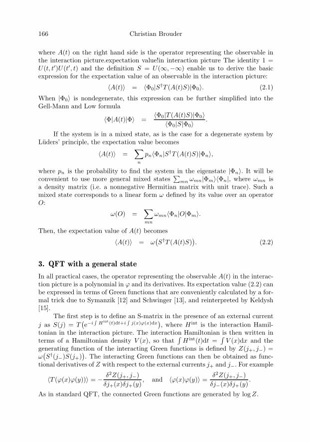
166 Christian Brouder
where A(t) on the right hand side is the operator representing the observable inthe interaction picture.expectation value!in interaction picture The identity 1 =U(t, t′)U(t′, t) and the definition S = U(∞,−∞) enable us to derive the basicexpression for the expectation value of an observable in the interaction picture:
〈A(t)〉 = 〈Φ0|S†T (A(t)S)|Φ0〉. (2.1)
When |Φ0〉 is nondegenerate, this expression can be further simplified into theGell-Mann and Low formula
〈Φ|A(t)|Φ〉 =〈Φ0|T (A(t)S)|Φ0〉
〈Φ0|S|Φ0〉.
If the system is in a mixed state, as is the case for a degenerate system byLuders’ principle, the expectation value becomes
〈A(t)〉 =∑
n
pn〈Φn|S†T (A(t)S)|Φn〉,
where pn is the probability to find the system in the eigenstate |Φn〉. It will beconvenient to use more general mixed states
∑mn ωmn|Φm〉〈Φn|, where ωmn is
a density matrix (i.e. a nonnegative Hermitian matrix with unit trace). Such amixed state corresponds to a linear form ω defined by its value over an operatorO:
ω(O) =∑mn
ωmn〈Φn|O|Φm〉.
Then, the expectation value of A(t) becomes
〈A(t)〉 = ω(S†T (A(t)S)
). (2.2)
3. QFT with a general state
In all practical cases, the operator representing the observable A(t) in the interac-tion picture is a polynomial in ϕ and its derivatives. Its expectation value (2.2) canbe expressed in terms of Green functions that are conveniently calculated by a for-mal trick due to Symanzik [12] and Schwinger [13], and reinterpreted by Keldysh[15].
The first step is to define an S-matrix in the presence of an external currentj as S(j) = T
(e−i
∫Hint(t)dt+i
∫j(x)ϕ(x)dx
), where H int is the interaction Hamil-
tonian in the interaction picture. The interaction Hamiltonian is then written interms of a Hamiltonian density V (x), so that
∫H int(t)dt =
∫V (x)dx and the
generating function of the interacting Green functions is defined by Z(j+, j−) =ω(S†(j−)S(j+)
). The interacting Green functions can then be obtained as func-
tional derivatives of Z with respect to the external currents j+ and j−. For example
〈T (ϕ(x)ϕ(y))〉 = − δ2Z(j+, j−)δj+(x)δj+(y)
, and 〈ϕ(x)ϕ(y)〉 =δ2Z(j+, j−)δj−(x)δj+(y)
.
As in standard QFT, the connected Green functions are generated by logZ.
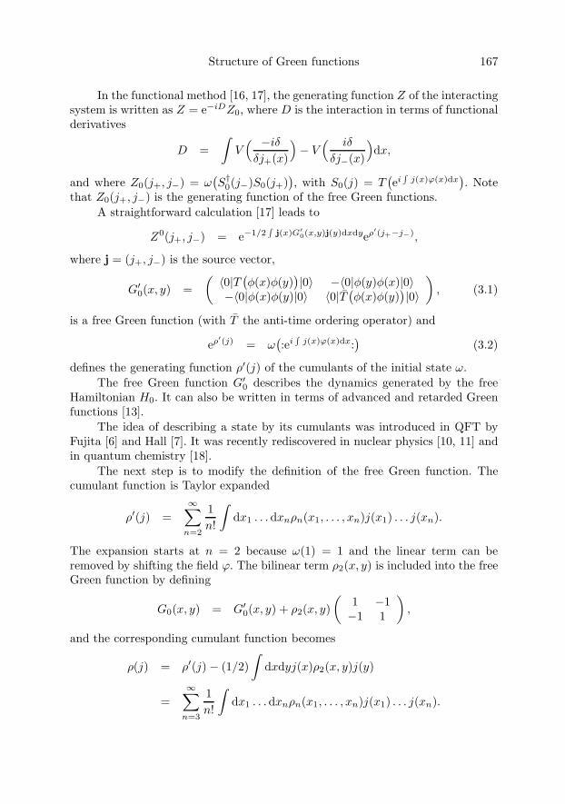
Structure of Green functions 167
In the functional method [16, 17], the generating function Z of the interactingsystem is written as Z = e−iDZ0, where D is the interaction in terms of functionalderivatives
D =∫
V( −iδδj+(x)
)− V
( iδ
δj−(x)
)dx,
and where Z0(j+, j−) = ω(S†
0(j−)S0(j+)), with S0(j) = T
(ei
∫j(x)ϕ(x)dx
). Note
that Z0(j+, j−) is the generating function of the free Green functions.A straightforward calculation [17] leads to
Z0(j+, j−) = e−1/2∫
j(x)G′0(x,y)j(y)dxdyeρ′(j+−j−),
where j = (j+, j−) is the source vector,
G′0(x, y) =
(〈0|T
(φ(x)φ(y)
)|0〉 −〈0|φ(y)φ(x)|0〉
−〈0|φ(x)φ(y)|0〉 〈0|T(φ(x)φ(y)
)|0〉
), (3.1)
is a free Green function (with T the anti-time ordering operator) and
eρ′(j) = ω(:ei
∫j(x)ϕ(x)dx:
)(3.2)
defines the generating function ρ′(j) of the cumulants of the initial state ω.The free Green function G′
0 describes the dynamics generated by the freeHamiltonian H0. It can also be written in terms of advanced and retarded Greenfunctions [13].
The idea of describing a state by its cumulants was introduced in QFT byFujita [6] and Hall [7]. It was recently rediscovered in nuclear physics [10, 11] andin quantum chemistry [18].
The next step is to modify the definition of the free Green function. Thecumulant function is Taylor expanded
ρ′(j) =∞∑
n=2
1n!
∫dx1 . . .dxnρn(x1, . . . , xn)j(x1) . . . j(xn).
The expansion starts at n = 2 because ω(1) = 1 and the linear term can beremoved by shifting the field ϕ. The bilinear term ρ2(x, y) is included into the freeGreen function by defining
G0(x, y) = G′0(x, y) + ρ2(x, y)
(1 −1−1 1
),
and the corresponding cumulant function becomes
ρ(j) = ρ′(j)− (1/2)∫
dxdyj(x)ρ2(x, y)j(y)
=∞∑
n=3
1n!
∫dx1 . . .dxnρn(x1, . . . , xn)j(x1) . . . j(xn).

168 Christian Brouder
Remark 3.1. There are several good reasons to use G0 and ρ instead of G′0 and ρ′:
(i) This modification is exactly what is done in solid-state physics when the freeGreen function includes a sum over occupied states [19]; (ii) At a fundamental level,G0 and ρ have a more intrinsic meaning than G′
0 and ρ′ because they do not dependon the state |0〉 chosen as the vacuum; (iii) An important theorem of quantum fieldtheory [20] states that, under quite general conditions, ρn(x1, . . . , xn) is a smoothfunction of its arguments when n > 2, so that G0 gathers all possible singularterms (a related result was obtained by Tikhodeev [21]); (iv) A state for whichρ(j) = 0 is called a quasi-free state [22], quasi-free states are very convenient inpractice because the rules of standard QFT can be used without basic changes.Thus, the additional complications arise precisely when ρ (and not ρ′) is not zero.
4. Nonperturbative equations
To size up the combinatorial complexity due to the presence of a non-zero ρ, wepresent the diagrammatic expansion of the one-body Green function G(x, y) forthe ϕ3 theory to second order in perturbation theory. For this illustrative purpose,it will be enough to say that the cumulant ρn(x1, . . . , xn) is pictured as a whitevertex with n edges attached to it, the other vertex of the edge is associated withone of the points x1, . . . , xn. For example, ρ4(x1, . . . , x4) is represented by thediagram In this diagram, the white dot does not stand for a spacetime point, it
just indicates that the points x1 to x4 are arguments of a common cumulant. If werestrict the calculation to the case when ρn = 0 if n is odd, we obtain the followingexpansion In standard QFT, only the first and last diagrams of the right hand side
G(x, y) = x y + + + + + +
+ + + + + + +
+ + + + + + + . . .
are present. In the general case when all ρn �= 0, the number of diagrams is stillmuch larger.

Structure of Green functions 169
4.1. Generalized Dyson equation
As mentioned in the introduction, the only known result concerning the structureof Green functions with a general state was derived by Hall for the one-body Greenfunction G(x, y) [7]
G = (1−A)−1(G0 + C)(1 −B)−1(1 + ΣG).
In diagrammatic terms the quantities A, B, C and Σ are sums of one-particleirreducible diagrams. If we take our example of the Green function of ϕ3 theoryup to second order, we find
In standard QFT, we have A = B = C = 0 and the diagrammatic represen-tation of Σ contains much less terms. However, the difference with standard QFTis not only limited to the number of diagrams. The definition (3.2) of the cumu-lant function, and the fact that the free field ϕ is a solution of the Klein-Gordonequation imply that ρn is a solution of the Klein-Gordon equation in each of itsvariables. Thus, A(x, y), B(x, y) and C(x, y) are solutions of the Klein-Gordonequation for x and y. As a consequence, applying the Klein-Gordon operator tothe Green function gives us (�+m2)G = (1−B)−1(1+ΣG). In other words, apply-ing the Klein-Gordon operator kills a large number of terms of G. This is in starkcontrast with standard QFT, where (�+m2)G = 1+ΣG and amputating a Greenfunction does not modify its structure. This important difference makes some toolsof standard QFT (e.g. amputated diagrams or Legendre transformation) invalidin the presence of a general state.
All those difficulties explain the scarcity of results available in non-pertur-bative QFT with a general state. Apart from Hall’s work [7], the only non-perturbative results are Tikhodeev’s cancellation theorems [23, 24] and the equa-tion of motion for the Green functions [25].
In the next section, we present a simple trick to derive the structure of Greenfunctions with a general state.

170 Christian Brouder
4.2. Quadrupling the sources
We first determine the main formal difference between standard QFT and QFTwith a general state. In both cases, the generating function of the Green functionscan be written Z = e−iDZ0, where D describes the interaction and Z0 the initialstate. In the presence of a general state, the interaction D is simple but Z0 is madenon standard by the cumulant factor eρ. The idea of the solution is to transferthe cumulant function ρ from Z0 to D, because powerful functional methods weredeveloped to deal with general interactions D. These methods were first proposedby Dominicis and Englert [26] and greatly expanded by the Soviet school [27, 28,29, 30, 31, 32, 33, 34, 35].
This transfer from the initial state to the interaction can be done easily byintroducing two additional external sources k+ and k− and using the identity
eρ(j+−j−) = eρ(−i δδk+
−i δδk− )ei
∫(j+(x)k+(x)−j−(x)k−(x))dx
∣∣k+=k−=0
.
The term involving ρ can now be transferred from Z0 to D by defining the newgenerating function
Z(j±, k±) = e−iDZ0(j±, k±),
where the modified interaction is
D =∫
V( −iδδj+(x)
)− V
( iδ
δj−(x)
)dx− iρ(−i δ
δk+− i
δ
δk−),
and the modified free generating function is
Z0(j±, k±) = e−1/2∫
J(x)G0(x,y)J(y)dxdy,
with J = (j+, j−, k+, k−). The modified free Green function G0 is now a 4x4 matrixthat can be written as a 2x2 matrix of 2x2 matrices
G0 =(
G0 −i1−i1 0
).
In contrast to the standard case, the free Green function G0 is invertible
G−10 =
(0 i1i1 G0
),
and it is again possible to use amputated diagrams and Legendre transformations.The free generating function Z0 is the exponential of a function that is bilinear inthe sources, and all the standard structural tools of QFT are available again. Weillustrate this by recovering Hall’s analogue of the Dyson equation.
4.3. An algebraic proof of Hall’s equation
The free generating function Z0 has a standard form and the Dyson equation holdsagain: G = G0 + G0ΣG, where G is the 4x4 one-body Green function obtained
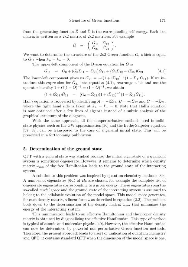
Structure of Green functions 171
from the generating function Z and Σ is the corresponding self-energy. Each 4x4matrix is written as a 2x2 matrix of 2x2 matrices. For example
G =(
G11 G12
G21 G22
).
We want to determine the structure of the 2x2 Green function G, which is equalto G11 when k+ = k− = 0.
The upper-left component of the Dyson equation for G is
G11 = G0 + (G0Σ11 − iΣ21)G11 + (G0Σ12 − iΣ22)G21. (4.1)
The lower-left component gives us G21 = −i(1 + iΣ12)−1(1 + Σ11G11). If we in-troduce this expression for G21 into equation (4.1), rearrange a bit and use theoperator identity 1 + O(1−O)−1 = (1−O)−1, we obtain
(1 + iΣ21)G11 = (G0 − Σ22)(1 + iΣ12)−1(1 + Σ11G11).
Hall’s equation is recovered by identifying A = −iΣ21, B = −iΣ12 and C = −Σ22,where the right hand side is taken at k+ = k− = 0. Note that Hall’s equationis now obtained after a few lines of algebra instead of a subtle analysis of thegraphical structure of the diagrams.
With the same approach, all the nonperturbative methods used in solid-state physics, such as the GW approximation [36] and the Bethe-Salpeter equation[37, 38], can be transposed to the case of a general initial state. This will bepresented in a forthcoming publication.
5. Determination of the ground state
QFT with a general state was studied because the initial eigenstate of a quantumsystem is sometimes degenerate. However, it remains to determine which densitymatrix ωmn of the free Hamiltonian leads to the ground state of the interactingsystem.
A solution to this problem was inspired by quantum chemistry methods [39].A number of eigenstates |Φn〉 of H0 are chosen, for example the complete list ofdegenerate eigenstates corresponding to a given energy. These eigenstates span theso-called model space and the ground state of the interacting system is assumed tobelong to the adiabatic evolution of the model space. This model space generates,for each density matrix, a linear form ω as described in equation (2.2). The problemboils down to the determination of the density matrix ωmn that minimizes theenergy of the interacting system.
This minimization leads to an effective Hamiltonian and the proper densitymatrix is obtained by diagonalizing the effective Hamiltonian. This type of methodis typical of atomic and molecular physics [40]. However, the effective Hamiltoniancan now be determined by powerful non-perturbative Green function methods.Therefore, the present approach leads to a sort of unification of quantum chemistryand QFT: it contains standard QFT when the dimension of the model space is one,

172 Christian Brouder
it contains standard quantum chemistry (more precisely many-body perturbationtheory) when the Green functions are expanded perturbatively.
Therefore, the present approach might help developing some new nonpertur-bative methods in quantum chemistry. On the other hand, quantum chemistryhas accumulated an impressive body of results. The physics Nobel-prize winnerKenneth Wilson stated that [41] “Ab initio quantum chemistry is an emergingcomputational area that is fifty years ahead of lattice gauge theory.” Therefore,the experience gained in quantum chemistry can be used to solve some of theremaining problems of the present approach, such as the removal of the secularterms [14] to all order.
6. Conclusion
The present paper sketched a new method to determine the Green functions ofquantum field theory with a general state. The main idea is to transform thecumulant function describing the initial state into an interaction term. As a conse-quence, the cumulants become dressed by the interaction, providing a much betterdescription of the correlation in the system.
An alternative method would be to work at the operator level, as was donerecently by Dutsch and Fredenhagen [42], and to take the expectation value at theend of the calculation. This would have the obvious advantage of dealing with afully rigorous theory. However, we would loose the non-perturbative aspects of thepresent approach.
Although this approach seems promising, much remains to be done before itcan be applied to realistic systems: (i) our description is purely formal; (ii) thedegenerate initial eigenstates lead to secular terms that must be removed [14];(iii) renormalization must be included, although this will probably not be verydifferent from the standard case, because all the singularities of the free systemare restricted to G0.
Interesting connections can be made with other problems. For example, thecancellation theorem [23] seems to be interpretable as a consequence of the uni-tarity of the S-matrix. It would extend Veltman’s largest time equation [43] to thecase of spacetime points with equal time. Another exciting track would be a con-nection with noncommutative geometry. Keldysh [15] noticed that the doubling ofsources could be replaced by a doubling of spacetime points. In other words, j±(x)becomes j(x±), where x± are two copies of the spacetime point x: time travelsfrom the past to the future for x+ and in the other direction for x−. Sivasubra-manian and coll. [44] have proposed to interpret this doubling of spacetime pointsin terms of noncommutative geometry. It would be interesting to follow this trackfor our quadrupling of spacetime points.
From the practical point of view, the main applications of our scheme willbe for the calculation of strongly-correlated systems, in particular for the optical
Structure of Green functions 173
response of some materials, such as gemstones, that remain beyond the reach ofthe standard tools of contemporary solid-state physics.
After the completion of this work, we came across a little known article bySergey Fanchenko, where the cumulants are used to define an effective action [45].His paper is also interesting because it gives a path integral formulation of quantumfield theory with a general state. His approach and the one of the present paperprovide complementary tools to attack nonperturbative problems of quantum fieldtheory with a general state.
Acknowledgement
I thank Alessandra Frabetti, Frederic Patras, Sergey Fanchenko and Pierre Cartierfor very useful discussions.
References
[1] F. J. Dyson. Heisenberg operators in quantum electrodynamics. I. Phys. Rev. 82(1951), 428–39.
[2] F. J. Dyson. Heisenberg operators in quantum electrodynamics. II. Phys. Rev. 83(1951), 608–27.
[3] M. Gell-Mann and F. Low. Bound states in quantum field theory. Phys. Rev. 84(1951), 350–4.
[4] A. L. Fetter and J. D. Walecka. Quantum Theory of Many-Particle Systems.McGraw-Hill, Boston (1971).
[5] E. K. U. Gross, E. Runge and O. Heinonen. Many-Particle Theory. Adam Hilger,Bristol (1991).
[6] S. Fujita. Introduction to Non Equilibrium Quantum Statistical Mechanics. Saunders,Philadelphia (1966).
[7] A. G. Hall. Non-equilibrium Green functions: Generalized Wick’s theorem and di-agrammatic perturbation theory with initial correlations. J. Phys. A: Math. Gen. 8(1975), 214–25.
[8] D. M. Esterling and R. V. Lange. Degenerate mass operator perturbation theory inthe Hubbard model. Rev. Mod. Phys. 40 (1968), 796–9.
[9] I. Lindgren, B. Asen, S. Salomonson and A.-M. Martensson-Pendrill. QED procedureapplied to the quasidegenerate fine-structure levels of He-like ions. Phys. Rev. A 64(2001), 062505.
[10] P. A. Henning. On the treatment of initial correlations in quantum field theory ofnon-equilibrium states. Nucl. Phys. B 337 (1990), 547–68.
[11] R. Fauser and H. H. Wolter. Non-equilibrium quantum field theory and perturbationtheory. Nucl. Phys. A 584 (1995), 604–620.
[12] K. Symanzik. On the many-body structure of Green’s functions in quantum fieldtheory. J. Math. Phys. 1 (1960), 249–73.
[13] J. Schwinger. Brownian motion of a quantum oscillator. J. Math. Phys. 2 (1961),407–32.
174 Christian Brouder
[14] Y. A. Kukharenko and S. G. Tikhodeev. Diagram technique in the theory of relax-ation processes. Soviet Phys. JETP 56 (1982), 831–8.
[15] L. V. Keldysh. Diagram technique for nonequilibrium processes. Soviet Phys. JETP20 (1965), 1018–26.
[16] J. Schwinger. On the Green’s functions of quantized fields. I. Proc. Nat. Acad. Sci.37 (1951), 452–5.
[17] K.-C. Chou, Z.-B. Su, B.-L. Hao and L. Yu. Equilibrium and nonequilibrium for-malisms made unified. Phys. Repts. 118 (1985), 1–131.
[18] W. Kutzelnigg and D. Mukherjee. Cumulant expansion of the reduced density ma-trices. J. Chem. Phys. 110 (1999), 2800–9.
[19] C. Brouder. Matrix elements of many-body operators and density correlations. Phys.Rev. A 72 (2005), 032720.
[20] S. Hollands and W. Ruan. The state space of perturbative quantum field theory incurved spacetimes. Ann. Inst. Henri Poincare 3 (2003), 635–57.
[21] S. G. Thikhodeev. Relations between many-body Green’s functions and correlationfunctions. Sov. Phys. Doklady 27 (1982), 492–3.
[22] B. S. Kay and R. M. Wald. Theorems on the uniqueness and thermal propertiesof stationary, nonsingular, quasifree states on spacetimes with a bifurcate Killinghorizon. Phys. Repts. 207 (1991), 49–136.
[23] S. G. Thikhodeev. On the vanishing of correlation-connected diagrams in Hall’s di-agram technique. Sov. Phys. Doklady 27 (1982), 624–5.
[24] P. Danielewicz. Quantum theory of nonequilibrium processes, I. Ann. Phys. 152(1984), 239–304.
[25] C. Brouder. Green function hierarchy for open shells. Euro. Phys. Lett. 71 (2005),556–62.
[26] C. de Dominicis and F. Englert. Potential-correlation function duality in statisticalphysics. J. Math. Phys. 8 (1967), 2143–6.
[27] A. N. Vasil’ev and A. K. Kazanskii. Legendre transforms of the generating functionalsin quantum field theory. Theor. Math. Phys. 12 (1972), 875–87.
[28] A. N. Vasil’ev and A. K. Kazanskii. Equations of motion for a Legendre transformof arbitrary order. Theor. Math. Phys. 14 (1973), 215–226.
[29] A. N. Vasil’ev, A. K. Kazanskii and Y. M. Pis’mak. Diagrammatic analysis of thefourth Legendre transform. Theor. Math. Phys. 20 (1974), 754–62.
[30] A. N. Vasil’ev, A. K. Kazanskii and Y. M. Pis’mak. Equations for higher Legendretransforms in terms of 1-irreducible vertices. Theor. Math. Phys. 19 (1974), 443–53.
[31] A. N. Vasil’ev. The field theoretic renormalization group in critical behavior theoryand stochastic dynamics. Chapman and Hall/CRC, New York (2004).
[32] Y. M. Pis’mak. Proof of the 3-irreducibility of the third Legendre transform. Theor.Math. Phys. 18 (1974), 211–8.
[33] Y. M. Pis’mak. Combinatorial analysis of the overlapping problem for vertices withmore than four legs. Theor. Math. Phys. 24 (1975), 649–58.
[34] Y. M. Pis’mak. Combinatorial analysis of the overlapping problem for vertices withmore than four legs: II Higher Legendre transforms. Theor. Math. Phys. 24 (1975),755–67.

Structure of Green functions 175
[35] Y. M. Pis’mak. n-particle problem in quantum field theory and the functional Le-gendre transforms. Int. J. Mod. Phys. 7 (1992), 2793–808.
[36] F. Aryasetiawan and O. Gunnarson. The GW method. Rep. Prog. Phys. 61 (1998),237–312.
[37] S. Albrecht, L. Reining, R. D. Sole and G. Onida. Ab initio calculation of excitoniceffects in the optical spectra of semiconductors. Phys. Rev. Lett. 80 (1998), 4510–3.
[38] L. X. Benedict, E. L. Shirley and R. B. Bohn. Optical absorption of insulators andthe electron-hole interaction: An ab initio calculation. Phys. Rev. Lett. 80 (1998),4514–7.
[39] C. Brouder. Many-body approach to crystal field theory. Phys. Stat. Sol. (c) 2 (2005),472–5.
[40] I. Lindgren and J. Morrison. Atomic Many-Body Theory. Second edition. Springer-Verlag, (1986).
[41] K. G. Wilson. Ab initio quantum chemistry: A source of ideas for lattice gauge the-orists. Nucl. Phys. Suppl. 17 (1990), 82–92.
[42] M. Dutsch and K. Fredenhagen. Causal perturbation theory in terms of retardedproducts, and a proof of the Action Ward Identity. Rev. Math. Phys. 16 (2004),1291–348.
[43] M. Veltman. Unitarity and causality in a renormalizable field theory with unstableparticles. Physica 29 (1963), 186–207.
[44] S. Sivasubramanian, Y. N. Srivastava, G. Vitiello and A. Widom. Quantum dissipa-tion induced noncommutative geometry. Phys. Lett. A 311 (2003), 97–105.
[45] S. S. Fanchenko. Generalized diagram technique of nonequilibrium processes. Theor.Math. Phys. 55 (1983), 406–9.
Christian BrouderInstitut de Mineralogie et de Physique des Milieux CondensesCNRS UMR7590, Universite Paris 6140 rue de LourmelFR–75015 Parise-mail: [email protected]

Quantum Field TheoryB. Fauser, J. Tolksdorf and E. Zeidler, Eds., 177–196c© 2009 Birkhauser Verlag Basel/Switzerland
The Quantum Action Principle in theFramework of Causal Perturbation Theory
Ferdinand Brennecke and Michael Dutsch
Abstract. In perturbative quantum field theory the maintenance of classicalsymmetries is quite often investigated by means of algebraic renormalization,which is based on the Quantum Action Principle. We formulate and prove thisprinciple in a new framework, in causal perturbation theory with localizedinteractions. Throughout this work a universal formulation of symmetries isused: the Master Ward Identity.
Mathematics Subject Classification (2000). Primary 81T15; Secondary 70S10;81T50.
Keywords. Perturbative renormalization, quantum action principle, masterWard identity, symmetries, causal perturbation theory, local fields.
1. Introduction
The main problem in perturbative renormalization is to prove that symmetries ofthe underlying classical theory can be maintained in the process of renormalization.In traditional renormalization theory this is done by ’algebraic renormalization’[26]. This method relies on the ’Quantum Action Principle’ (QAP), which is due toLowenstein [23] and Lam [22]. This principle states that the most general violationof an identity expressing a relevant symmetry (’Ward identity’) can be expressedby the insertion of a local field with appropriately bounded mass dimension. Pro-ceeding in a proper field formalism1 by induction on the order of �, this knowledgeabout the structure of violations of Ward identities and often cohomological re-sults are used to remove these violations by finite renormalizations. For example,this method has been used to prove BRST-symmetry of Yang-Mills gauge theories[2, 3, 31, 17, 1].
1By ’proper field formalism’ we mean the description of a perturbative QFT in terms of thegenerating functional of the 1-particle irreducible diagrams.
178 Ferdinand Brennecke and Michael Dutsch
Traditionally, algebraic renormalization is formulated in terms of a renormal-ization method in which the interaction is not localized (i.e. Sint =
∫dxLint(x) ,
where Lint is a polynomial in the basic fields with constant coefficients), for ex-ample the BPHZ momentum space subtraction procedure [32, 23, 22] or the polesubtractions of dimensionally regularized integrals [5]. In [25] it is pointed out(without proof) that the QAP is a general theorem in perturbative QFT for non-localized interactions, i.e. it holds in any renormalization scheme.2
However, for the generalization of perturbative QFT to general globally hy-perbolic curved space-times, it is advantageous to work with localized interactions(i.e. Sint =
∫dx
∑n≥1(g(x))n Lint,n(x) , where g is a test function with compact
support) and to use a renormalization method which proceeds in configurationspace and in which the locality and causality of perturbative QFT is clearly visible[8, 18, 19]. It is causal perturbation theory (CPT) [4, 15, 14] which is distinguishedby these criteria.
Since it is the framework of algebraic QFT [16] in which the problems specificfor curved space-times (which mainly rely on the absence of translation invariance)can best be treated, our main goal is the perturbative construction of the net oflocal algebras of interacting fields (’perturbative algebraic QFT’). Using the for-mulation of causality in CPT, it was possible to show that for this constructionit is sufficient to work with localized interactions [8, 12]. Hence, a main argu-ment against localized interactions, namely that a space or time dependence ofthe coupling constants has not been observed in experiments, does not concernperturbative algebraic QFT. Because of the localization of the interactions, theconstruction of the local algebras of interacting fields is not plagued by infrareddivergences, the latter appear only in the construction of physical states.
Due to these facts it is desirable to transfer the techniques of algebraic renor-malization to CPT, that is to formulate the �-expansion, a proper field formalismand the QAP in the framework of CPT. For the �-expansion the difficulty is thatCPT is a construction of the perturbation series by induction on the coupling con-stant, a problem solved in [11, 12]. A formulation of the QAP in the frameworkof CPT has partially been given in [11] and in [27]; but for symmetries relyingon a variation of the fields (as e.g. BRST-symmetry) an appropriate formulationand a proof were missing up to the appearance of the paper [6]. In the latter,also a proper field formalism and algebraic renormalization are developed in theframework of CPT.
In this paper we concisely review main results of that work [6], putting thefocus on the QAP. To be closer to the conventional treatment of perturbative QFTin Minkowski space and to simplify the formalism, we work with the Wightman 2-point function instead of a Hadamard function.3 Compared with [6], we formulatesome topics alternatively, in particular we introduce the proper field formalism
2Causal perturbation theory, with the adiabatic limit carried out, is included in that statement.3In [6] smoothness in the mass m is required for m ≥ 0 which excludes the Wightman 2-pointfunction.

Quantum Action Principle in Causal Perturbation Theory 179
without using arguments relying on Wick’s theorem and the corresponding dia-grammatic interpretation. In addition we prove a somewhat stronger version ofthe QAP.
The validity of the QAP is very general. Therefore, we investigate a universalformulation of Ward identities: the Master Ward Identity (MWI) [9, 13]. Thisidentity can be derived in the framework of classical field theory simply from thefact that classical fields can be multiplied pointwise. Since this is impossible forquantum fields (due to their distributional character), the MWI is a highly non-trivial renormalization condition, which cannot be fulfilled in general, the wellknown anomalies of perturbative QFT are the obstructions.
2. The off-shell Master Ward Identity in classical field theory
For algebraic renormalization it is of crucial importance that the considered Wardidentities hold true in classical field theory. Therefore, in this section, we derive theoff-shell MWI in the classical framework. The formalism of classical field theory,which we are going to introduce, will be used also in perturbative QFT, since thelatter will be obtained by deformation of the classical Poisson algebra (Sect. 3)[11, 12, 13, 14].
For simplicity we study the model of a real scalar field ϕ on d dimensionalMinkowski space M, d > 2. The field ϕ and partial derivatives ∂aϕ (a ∈ Nd
0) areevaluation functionals on the configuration space C ≡ C∞(M,R) : (∂aϕ)(x)(h) =∂ah(x). Let F be the space of all functionals
F (ϕ) : C −→ C , F (ϕ)(h) = F (h) , (2.1)
which are localized polynomials in ϕ:
F (ϕ) =N∑
n=0
∫dx1 . . . dxn ϕ(x1) · · ·ϕ(xn)fn(x1, . . . , xn) , (2.2)
where N < ∞ and the fn’s are C-valued distributions with compact support,which are symmetric under permutations of the arguments and whose wave frontsets satisfy the condition
WF(fn) ∩(Mn × (V
n
+ ∪ Vn
−))
= ∅ (2.3)
and f0 ∈ C. (V ± denotes the closure of the forward/backward light-cone.) En-dowed with the classical product (F1 ·F2)(h) := F1(h) ·F2(h), the space F becomesa commutative algebra. By the support of a functional F ∈ F we mean the supportof δF
δϕ .The space of local functionals Floc ⊂ F is defined as
Flocdef=
{∫dx
N∑i=1
Ai(x)hi(x) ≡N∑
i=1
Ai(hi) |Ai ∈ P , hi ∈ D(M)}
, (2.4)
180 Ferdinand Brennecke and Michael Dutsch
where P is the linear space of all polynomials of the field ϕ and its partial deriva-tives:
P :=∨{
∂aϕ | a ∈ Nd0
}. (2.5)
We consider action functionals of the form Stot = S0 + λS where S0def=∫
dx12 (∂μϕ∂
μϕ − m2ϕ2) is the free action, λ a real parameter and S ∈ F somecompactly supported interaction, which may be non-local. The retarded Greenfunction Δret
Stotcorresponding to the action Stot, is defined by∫
dy ΔretStot
(x, y)δ2Stot
δϕ(y)δϕ(z)= δ(x− z) =
∫dy
δ2Stot
δϕ(x)δϕ(y)Δret
Stot(y, z) (2.6)
and ΔretStot
(x, y) = 0 for x sufficiently early. In the following we consider onlyactions Stot for which the retarded Green function exists and is unique in thesense of formal power series in λ.
To introduce the perturbative expansion around the free theory and to definethe Peierls bracket, we define retarded wave operators which map solutions of thefree theory to solutions of the interacting theory [13]. However, we define them asmaps on the space C of all field configurations (’off-shell formalism’) and not onlyon the space of free solutions:
Definition 2.1. A retarded wave operator is a family of maps (rS0+S,S0)S∈F fromC into itself with the properties
(i) rS0+S,S0(f)(x) = f(x) for x sufficiently early(ii) δ(S0+S)
δϕ ◦ rS0+S,S0 = δS0δϕ .
The following Lemma is proved in [6].
Lemma 2.2. The retarded wave operator (rS0+S,S0)S∈F exists and is unique andinvertible in the sense of formal power series in the interaction S.
Motivated by the interaction picture known from QFT, we introduce retardedfields: the classical retarded field to the interaction S and corresponding to thefunctional F ∈ F is defined by
F clS
def= F ◦ rS0+S,S0 : C −→ C. (2.7)
The crucial factorization property,
(F ·G)clS = F clS ·Gcl
S , (2.8)
cannot be maintained in the process of quantization, because quantum fields aredistributions. This is why many proofs of symmetries in classical field theory donot apply to QFT (cf. Sect. 5).
The perturbative expansion around the free theory is defined by expandingthe retarded fields with respect to the interaction. The coefficients are given bythe classical retarded product Rcl [13]:
Rcl : TF ⊗ F → F , Rcl(S⊗n, F ) def=dn
dλn
∣∣∣λ=0
F ◦ rS0+λS,S0 , (2.9)
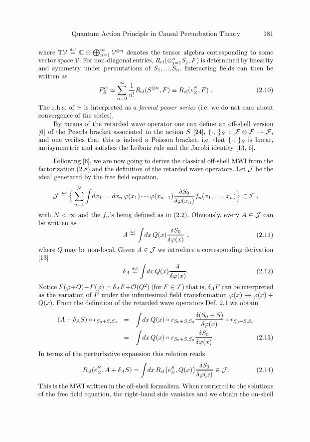
Quantum Action Principle in Causal Perturbation Theory 181
where TV def= C ⊕⊕∞
n=1 V⊗n denotes the tensor algebra corresponding to somevector space V . For non-diagonal entries, Rcl(⊗n
j=1Sj , F ) is determined by linearityand symmetry under permutations of S1, ..., Sn. Interacting fields can then bewritten as
F clS �
∞∑n=0
1n!Rcl(S⊗n, F ) ≡ Rcl(eS
⊗, F ) . (2.10)
The r.h.s. of � is interpreted as a formal power series (i.e. we do not care aboutconvergence of the series).
By means of the retarded wave operator one can define an off-shell version[6] of the Peierls bracket associated to the action S [24], {·, ·}S : F ⊗ F → F ,and one verifies that this is indeed a Poisson bracket, i.e. that {·, ·}S is linear,antisymmetric and satisfies the Leibniz rule and the Jacobi identity [13, 6].
Following [6], we are now going to derive the classical off-shell MWI from thefactorization (2.8) and the definition of the retarded wave operators. Let J be theideal generated by the free field equation,
J def={ N∑
n=1
∫dx1 . . . dxn ϕ(x1) · · ·ϕ(xn−1)
δS0
δϕ(xn)fn(x1, . . . , xn)
}⊂ F ,
with N < ∞ and the fn’s being defined as in (2.2). Obviously, every A ∈ J canbe written as
Adef=
∫dxQ(x)
δS0
δϕ(x), (2.11)
where Q may be non-local. Given A ∈ J we introduce a corresponding derivation[13]
δAdef=
∫dxQ(x)
δ
δϕ(x). (2.12)
Notice F (ϕ+Q)−F (ϕ) = δAF+O(Q2) (for F ∈ F) that is, δAF can be interpretedas the variation of F under the infinitesimal field transformation ϕ(x) �→ ϕ(x) +Q(x). From the definition of the retarded wave operators Def. 2.1 we obtain
(A + δAS) ◦ rS0+S,S0 =∫dxQ(x) ◦ rS0+S,S0
δ(S0 + S)δϕ(x)
◦ rS0+S,S0
=∫dxQ(x) ◦ rS0+S,S0
δS0
δϕ(x). (2.13)
In terms of the perturbative expansion this relation reads
Rcl(eS⊗, A + δAS) =
∫dxRcl
(eS⊗, Q(x)
) δS0
δϕ(x)∈ J . (2.14)
This is the MWI written in the off-shell formalism. When restricted to the solutionsof the free field equation, the right-hand side vanishes and we obtain the on-shell
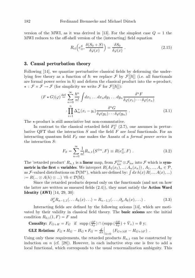
182 Ferdinand Brennecke and Michael Dutsch
version of the MWI, as it was derived in [13]. For the simplest case Q = 1 theMWI reduces to the off-shell version of the (interacting) field equation
Rcl
(eS⊗,
δ(S0 + S)δϕ(x)
)=
δS0
δϕ(x). (2.15)
3. Causal perturbation theory
Following [14], we quantize perturbative classical fields by deforming the under-lying free theory as a function of �: we replace F by F [[�]] (i.e. all functionalsare formal power series in �) and deform the classical product into the �-product,� : F × F → F (for simplicity we write F for F [[�]]):
(F � G)(ϕ) def=∞∑
n=0
�n
n!
∫dx1 . . . dxndy1 . . . dyn
δnF
δϕ(x1) · · · δϕ(xn)
·n∏
i=1
Δ+m(xi − yi)
δnG
δϕ(y1) · · · δϕ(yn). (3.1)
The �-product is still associative but non-commutative.In contrast to the classical retarded field F cl
S (2.7), one assumes in pertur-bative QFT that the interaction S and the field F are local functionals. For aninteracting quantum field FS one makes the Ansatz of a formal power series inthe interaction S:
FS =∞∑
n=0
1n!Rn,1
(S⊗n, F
)≡ R(eS
⊗, F ) . (3.2)
The ’retarded product’ Rn,1 is a linear map, from F⊗nloc ⊗Floc into F which is sym-
metric in the first n variables. We interpret R(A1(x1), ...;An(xn)) , A1, ..., An ∈ P ,as F -valued distributions onD(Mn), which are defined by:
∫dxh(x)R(..., A(x), ...)
:= R(...⊗A(h)⊗ ...) ∀h ∈ D(M).Since the retarded products depend only on the functionals (and not on how
the latter are written as smeared fields (2.4)), they must satisfy the Action WardIdentity (AWI) [14, 29, 30]:
∂xμRn−1,1(. . . Ak(x) . . .) = Rn−1,1(. . . , ∂μAk(x), . . .) . (3.3)
Interacting fields are defined by the following axioms [14], which are moti-vated by their validity in classical field theory. The basic axioms are the initialcondition R0,1(1, F ) = F and
Causality: FG+H = FG if supp ( δFδϕ ) ∩ (supp ( δH
δϕ ) + V+) = ∅ y;
GLZ Relation: FG � HG −HG � FG = ddλ
∣∣∣λ=0
(FG+λH −HG+λF ) .
Using only these requirements, the retarded products Rn,1 can be constructed byinduction on n (cf. [28]). However, in each inductive step one is free to add alocal functional, which corresponds to the usual renormalization ambiguity. This

Quantum Action Principle in Causal Perturbation Theory 183
ambiguity is reduced by imposing renormalization conditions as further axioms,see below.
Mostly, perturbative QFT is formulated in terms of the time ordered product(’T -product’) T : TFloc → F , which is a linear and totally symmetric map.Compared with the R-product, the T -product has the advantage of being totallysymmetric and the disadvantage that its classical limit does not exist [11]. R- andT -products are related by Bogoliubov’s formula:
R(eS⊗ , F
)=
�iS(S)−1 �
d
dτ
∣∣∣τ=0
S(S + τF ) , (3.4)
where
S(S) ≡ T(e
iS/�⊗
)≡
∞∑n=0
in
n!�nTn(S⊗n) . (3.5)
The basic axioms for retarded products translate into the following basic axioms forT -products: the initial conditions T0(1) = 1, T1(F ) = F and causal factorization:
Tn(A1(x1), ..., An(xn)) =
Tk(A1(x1), ..., Ak(xk)) � Tn−k(Ak+1(xk+1), ..., An(xn)) (3.6)
if {x1, ..., xk} ∩ ({xk+1, ..., xn}+ V−) = ∅. There is no axiom corresponding to theGLZ Relation. The latter can be interpreted as ’integrability condition’ for the’vector potential’ R
(eS⊗ , F
), that is it ensures the existence of the ’potential’ S(S)
fulfilling (3.4); for details see [7] and Proposition 2 in [10].For this paper the following renormalization conditions are relevant (besides
the MWI).Translation Invariance: The group (Rd,+) of space and time translations has
an obvious automorphic action β on F , which is determined by βaϕ(x) =ϕ(x + a) , a ∈ Rd. We require
βa S(S) = S(βaS) , ∀a ∈ Rd . (3.7)
Field Independence: δTδϕ(x) = 0 . This axiom implies the causal Wick expansion
of [15] as follows [14]: since T (⊗nj=1Fj) ∈ F is polynomial in ϕ, it has a finite
Taylor expansion in ϕ. By using Field Independence, this expansion can bewritten as
Tn(A1(x1), · · · , An(xn)) =∑
l1,...,ln
1l1! · · · ln!
·Tn
(· · · ,
∑ai1...aili
∂liAi
∂(∂ai1ϕ) · · · ∂(∂ailiϕ)(xi), · · ·
)∣∣∣ϕ=0
n∏i=1
li∏ji=1
∂aijiϕ(xi) (3.8)
with multi-indices aiji ∈ Nd0.
Scaling: This requirement uses the mass dimension of a monomial in P , whichis defined by the conditions
dim(∂aϕ) =d− 2
2+ |a| and dim(A1A2) = dim(A1) + dim(A2) (3.9)

184 Ferdinand Brennecke and Michael Dutsch
for all monomials A1, A2 ∈ P . The mass dimension of a polynomial in Pis the maximum of the mass dimensions of the contributing monomials. Wedenote by Phom the set of all field polynomials which are homogeneous in themass dimension.
The axiom Scaling Degree requires that ’renormalization may not makethe interacting fields more singular’ (in the UV-region). Usually this is for-mulated in terms of Steinmann’s scaling degree [28]:
sd(f) def= inf{δ ∈ R | limρ↓0
ρδf(ρx) = 0}, f ∈ D′(Rk) or f ∈ D′(Rk \ {0}). (3.10)
Namely, one requires
sd(T (A1, ..., An)|ϕ=0(x1 − xn, ...)
)≤
n∑j=1
dim(Aj) , ∀Aj ∈ Phom , (3.11)
where Translation Invariance is assumed. Notice that this condition restrictsall coefficients in the causal Wick expansion (3.8).
In the inductive construction of the sequence (Rn−1,1)n∈N or (Tn)n∈N, respectively,the problem of renormalization appears as the extension of the coefficients in thecausal Wick expansion (which are C[[�]]-valued distributions) from D(Rd(n−1) \{0}) to D(Rd(n−1)). This extension has to be done in the sense of formal powerseries in �, that is individually in each order in �. With that it holds
lim�→0
R = Rcl . (3.12)
In [14] it is shown that there exists a T -product which fulfils all axioms. Thenon-uniqueness of solutions is characterized by the ’Main Theorem’; for a completeversion see [14].
4. Proper vertices
A main motivation for introducing proper vertices is to select that part of a T -product for which renormalization is non-trivial (cf. [21]). This is the contribu-tion of all 1-particle-irreducible (1PI) subdiagrams. This selection can be done asfollows: first one eliminates all disconnected diagrams. Then, one interprets eachconnected diagram as tree diagram with non-local vertices (’proper vertices’) givenby the 1PI-subdiagrams. The proper vertices can be interpreted as the ’quantumpart’ of the Feynman diagrams. Since renormalization is unique and trivial fortree diagrams, Ward identities can equivalently be formulated in terms of propervertices (Sect. 5.1).
Essentially we follow this procedure, however, we avoid to argue in terms ofdiagrams, i.e. to use Wick’s Theorem. It has been shown in [6] that with our defi-nition (4.6) of the vertex functional Γ the ’proper interaction’ Γ(eS
⊗) correspondsto the sum of all 1PI-diagrams of T (eiS/�
⊗ ).

Quantum Action Principle in Causal Perturbation Theory 185
The connected part T c of a time-ordered T can be defined recursively by [11]
T cn(⊗n
j=1Fj)def= Tn(⊗n
j=1Fj)−∑|P |≥2
∏J∈P
T c|J|(⊗j∈JFj) . (4.1)
It follows that T and T c are related by the linked cluster theorem:
T (eiF⊗ ) = exp•(T
c(eiF⊗ )) , (4.2)
where exp• denotes the exponential function with respect to the classical product.For F ∈ Floc the connected tree part T c
tree,n(F⊗n) can be defined as follows[11]: since T c
n = O(�n−1) , the limit
�−(n−1) T ctree,n
def= lim�→0
�−(n−1) T cn (4.3)
exists. This definition reflects the well known statements that T ctree is the ’classical
part’ of T c and that connected loop diagrams are of higher orders in �.Since proper vertices are non-local, we need the connected tree part
T ctree(⊗n
j=1Fj) for non-local entries Fj ∈ F . This can be defined recursively [6]:
T ctree(⊗n+1
j=1Fj) =n∑
k=1
∫dx1...dxk dy1...dyk
δkFn+1
δϕ(x1)...δϕ(xk)
·k∏
j=1
ΔFm(xj − yj)
1k!
∑I1�...�Ik={1,...,n}
δ
δϕ(y1)T c
tree(⊗j∈I1Fj) · ...
· δ
δϕ(yk)T c
tree(⊗j∈IkFj) , (4.4)
where Ij �= ∅ ∀j , ( means the disjoint union and ΔFm is the Feynman propagator
for mass m. (Note that in the sum over I1, ..., Ik the order of I1, ..., Ik is distin-guished and, hence, there is a factor 1
k! .) For local entries the two definitions (4.3)and (4.4) of T c
tree agree, as explained in [6].The ’vertex functional’ Γ is defined by the following proposition [6]:
Proposition 4.1. There exists a totally symmetric and linear map
Γ : TFloc → F (4.5)
which is uniquely determined by
T c(eiS/�⊗ ) = T c
tree
(e
iΓ(eS⊗)/�
⊗). (4.6)
To zeroth and first order in S we obtain
Γ(1) = 0 , Γ(S) = S . (4.7)
Since T c, T ctree and Γ are linear and totally symmetric, the defining relation (4.6)
implies
T c(eiS/�⊗ ⊗ F ) = T c
tree
(e
iΓ(eS⊗)/�
⊗ ⊗ Γ(eS⊗ ⊗ F )
). (4.8)
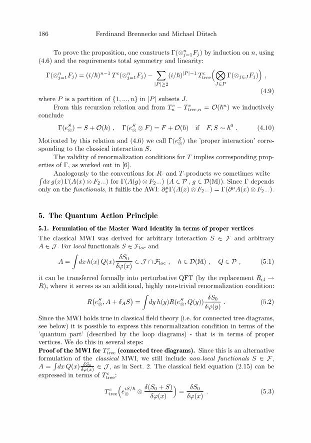
186 Ferdinand Brennecke and Michael Dutsch
To prove the proposition, one constructs Γ(⊗nj=1Fj) by induction on n, using
(4.6) and the requirements total symmetry and linearity:
Γ(⊗nj=1Fj) = (i/�)n−1 T c(⊗n
j=1Fj)−∑|P |≥2
(i/�)|P |−1 T ctree
(⊗J∈P
Γ(⊗j∈JFj)),
(4.9)where P is a partition of {1, ..., n} in |P | subsets J .
From this recursion relation and from T cn − T c
tree,n = O(�n) we inductivelyconclude
Γ(eS⊗) = S +O(�) , Γ(eS
⊗ ⊗ F ) = F +O(�) if F, S ∼ �0 . (4.10)
Motivated by this relation and (4.6) we call Γ(eS⊗) the ’proper interaction’ corre-sponding to the classical interaction S.
The validity of renormalization conditions for T implies corresponding prop-erties of Γ, as worked out in [6].
Analogously to the conventions for R- and T -products we sometimes write∫dx g(x) Γ(A(x) ⊗ F2...) for Γ(A(g)⊗ F2...) (A ∈ P , g ∈ D(M)). Since Γ depends
only on the functionals, it fulfils the AWI: ∂μxΓ(A(x)⊗F2...) = Γ(∂μA(x)⊗F2...).
5. The Quantum Action Principle
5.1. Formulation of the Master Ward Identity in terms of proper vertices
The classical MWI was derived for arbitrary interaction S ∈ F and arbitraryA ∈ J . For local functionals S ∈ Floc and
A =∫dxh(x)Q(x)
δS0
δϕ(x)∈ J ∩ Floc , h ∈ D(M) , Q ∈ P , (5.1)
it can be transferred formally into perturbative QFT (by the replacement Rcl →R), where it serves as an additional, highly non-trivial renormalization condition:
R(eS⊗, A + δAS
)=∫dy h(y)R(eS
⊗, Q(y))δS0
δϕ(y). (5.2)
Since the MWI holds true in classical field theory (i.e. for connected tree diagrams,see below) it is possible to express this renormalization condition in terms of the’quantum part’ (described by the loop diagrams) - that is in terms of propervertices. We do this in several steps:Proof of the MWI for T c
tree (connected tree diagrams). Since this is an alternativeformulation of the classical MWI, we still include non-local functionals S ∈ F ,A =
∫dxQ(x) δS0
δϕ(x) ∈ J , as in Sect. 2. The classical field equation (2.15) can beexpressed in terms of T c
tree:
T ctree
(e
iS/�⊗ ⊗ δ(S0 + S)
δϕ(x)
)=
δS0
δϕ(x). (5.3)
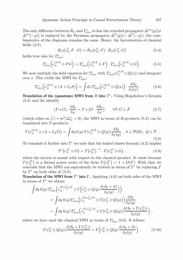
Quantum Action Principle in Causal Perturbation Theory 187
The only difference between Rcl and T ctree is that the retarded propagator Δret(y)(�=
Δret(−y)) is replaced by the Feynman propagator ΔF (y)(= ΔF (−y)), the com-binatorics of the diagrams remains the same. Hence, the factorization of classicalfields (2.8),
Rcl
(eS⊗, F ·G
)= Rcl
(eS⊗, F
)·Rcl
(eS⊗, G
)(5.4)
holds true also for T ctree:
T ctree
(e
iS/�⊗ ⊗ FG
)= T c
tree
(e
iS/�⊗ ⊗ F
)· T c
tree
(e
iS/�⊗ ⊗G
). (5.5)
We now multiply the field equation for T ctree with T c
tree(eiS/�⊗ ⊗Q(x)) and integrate
over x. This yields the MWI for T ctree:
T ctree
(e
iS/�⊗ ⊗ (A + δAS)
)=∫dxT c
tree
(e
iS/�⊗ ⊗Q(x)
)· δS0
δϕ(x). (5.6)
Translation of the (quantum) MWI from R into T c. Using Bogoliubov’s formula(3.4) and the identity
(F � G) · δS0
δϕ= F �
(G · δS0
δϕ
)∀F,G ∈ F (5.7)
(which relies on (� + m2)Δ+m = 0), the MWI in terms of R-products (5.2) can be
translated into T -products:
T(e
iS/�⊗ ⊗ (A + δAS)
)=∫dy h(y)T (eiS/�
⊗ ⊗Q(y))δS0
δϕ(y), h ∈ D(M) , Q ∈ P .
(5.8)To translate it further into T c we note that the linked cluster formula (4.2) implies
T c(eiF⊗ ⊗G
)= T
(eiF⊗)−1 · T
(eiF⊗ ⊗G
), (5.9)
where the inverse is meant with respect to the classical product. It exists becauseT(eiF⊗)
is a formal power series of the form T(eiF⊗)
= 1 + O(F ). With that weconclude that the MWI can equivalently be written in terms of T c by replacing Tby T c on both sides of (5.8).Translation of the MWI from T c into Γ. Applying (4.6) on both sides of the MWIin terms of T c we obtain∫
dy h(y)T ctree
(e
iΓ(eS⊗)/�
⊗ ⊗ Γ(eS⊗ ⊗Q(y)
δ(S0 + S)δϕ(y)
))=∫dy h(y)T c
tree
(e
iΓ(eS⊗)/�
⊗ ⊗ Γ(eS⊗ ⊗Q(y)
)) δS0
δϕ(y)
=∫dy h(y)T c
tree
(e
iΓ(eS⊗)/�
⊗ ⊗ Γ(eS⊗ ⊗Q(y))
δ(S0 + Γ(eS⊗))δϕ(y)
),
where we have used the classical MWI in terms of T ctree (5.6). It follows
Γ(eS⊗ ⊗Q(y))
δ(S0 + Γ(eS⊗))
δϕ(y)= Γ
(eS⊗ ⊗Q(y)
δ(S0 + S)δϕ(y)
). (5.10)

188 Ferdinand Brennecke and Michael Dutsch
The various formulations of the MWI, in terms of R-products (5.2), T -products(5.8), T c-products and in terms of proper vertices (5.10), they all are equivalent.
Remark 5.1. The off-shell field equation
T(e
iS/�⊗ ⊗ δ(S0 + S)
δϕ(y)
)=
δS0
δϕ(y)· T
(e
iS/�⊗
), ∀S , (5.11)
is a further renormalization condition, which can equivalently be expressed by
Γ(eS⊗ ⊗ ϕ(y)) = ϕ(y) , ∀S , (5.12)
as shown in [6]. For a T -product satisfying this condition and for Q = Dϕ (whereD is a polynomial in partial derivatives) the QAP simplifies to
Dϕ(y)δ(S0 + Γ(eS⊗))
δϕ(y)= Γ
(eS⊗ ⊗Dϕ(y)
δ(S0 + S)δϕ(y)
). (5.13)
5.2. The anomalous Master Ward Identity - Quantum Action Principle
The QAP is a statement about the structure of all possible violations of Wardidentities. In our framework the main statement of the QAP is that any termviolating the MWI can be expressed as Γ(eS⊗⊗Δ), where Δ is local (in a strongersense than only Δ ∈ Floc) and Δ = O(�) and the mass dimension of Δ is boundedin a suitable way.
Theorem 5.2 (Quantum Action Principle). (a) Let Γ be the vertex functional be-longing to a time ordered product satisfying the basic axioms and Translation In-variance (3.7). Then there exists a unique sequence of linear maps (Δn)n∈N,
Δn : P⊗(n+1) → D′(M,Floc) , ⊗nj=1Lj ⊗Q �→ Δn(⊗n
j=1Lj(xj);Q(y)) (5.14)
(D′(M,Floc) is the space of Floc-valued distributions on D(M)), which are sym-metric in the first n factors,
Δn(⊗nj=1Lπj(xπj);Q(y)) = Δn(⊗n
j=1Lj(xj);Q(y)) (5.15)
for all permutations π, and which are implicitly defined by the ’anomalous MWI’
Γ(eS⊗⊗Q(y))
δ(S0 + Γ(eS⊗))
δϕ(y)= Γ
(eS⊗⊗
(Q(y)
δ(S0 + S)δϕ(y)
+Δ(L;Q)(g; y)))
, (5.16)
where S = L(g) (L ∈ P , g ∈ D(M)) and
Δ(L;Q)(g; y) :=∞∑
n=0
1n!
∫dx1...dxn
n∏j=1
g(xj)Δn(⊗nj=1L(xj);Q(y)) . (5.17)
As a consequence of (5.16) the maps Δn have the following properties:
(i) Δ0 = 0 ;

Quantum Action Principle in Causal Perturbation Theory 189
(ii) locality: there exist linear maps Pna : P⊗(n+1) → P (where a runs through a
finite subset of (Nd0)
n), which are symmetric in the first n factors, such thatΔn can be written as
Δn(⊗nj=1Lj(xj);Q(y)) =
∑a∈(Nd
0)n
∂aδ(x1−y, ..., xn−y)Pna (⊗n
j=1Lj;Q)(y) . (5.18)
(iii) Δn(⊗nj=1Lj(xj);Q(y)) = O(�) ∀n > 0 if Lj ∼ �0, Q ∼ �0 .
(b) If the time ordered product satisfies the renormalization conditions FieldIndependence and Scaling Degree (3.11), then each term on the r.h.s. of (5.18)fulfils
|a|+ dim(Pna (⊗n
j=1Lj ;Q)) ≤n∑
j=1
dim(Lj) + dim(Q) +d + 2
2− dn . (5.19)
For a renormalizable interaction (that is dim(L) ≤ d) this implies
|a|+ dim(Pna (L⊗n;Q)) ≤ dim(Q) +
d + 22
. (5.20)
Note that (5.16) differs from the MWI (5.10) only by the local termΔ(L;Q)(g; y), which clearly depends on the chosen normalization of the time or-dered product. Therefore, Δ(L;Q)(g; y) = 0 is a sufficient condition for the validityof the MWI for Q and S = L(g); it is also necessary due to the uniqueness of themaps Δn.
Proof. (a) Proceeding as in Sect. 5.1, the defining relation (5.16) can equivalentlybe written in terms of T -products:
T(e
iS/�⊗ ⊗
(Q(y)
δ(S0 + S)δϕ(y)
+ Δ(L;Q)(g; y)))
= T(e
iS/�⊗ ⊗Q(y)
) δS0
δϕ(y). (5.21)
To n-th order in g this equation reads
Δn(L⊗n;Q(y))(g⊗n) = T((iS/�)⊗n ⊗Q(y)
)· δS0
δϕ(y)− T
((iS/�)⊗n ⊗Q(y)
δS0
δϕ(y)
)−nT
((iS/�)⊗n−1 ⊗Q(y)
δS
δϕ(y)
)−
n−1∑l=0
(n
l
)T((iS/�)⊗n−l ⊗Δl(L⊗l;Q(y))(g⊗l)
).
(5.22)

190 Ferdinand Brennecke and Michael Dutsch
Taking linearity and symmetry (5.15) into account we extend this relation to non-diagonal entries and write it in terms of the distributional kernels
Δn(⊗nj=1Lj(xj);Q(y)) =
( i
�
)n
T(⊗n
j=1Lj(xj)⊗Q(y))· δS0
δϕ(y)
−( i
�
)n
T(⊗n
j=1Lj(xj)⊗Q(y) · δS0
δϕ(y)
)−
n∑l=1
( i
�
)n−1
T(⊗j( �=l)Lj(xj)⊗Q(y)
∑a
(∂aδ)(xl − y)∂Ll
∂(∂aϕ)(xl)
)−
∑I⊂{1,...,n} , Ic �=∅
( i
�
)|Ic|T(⊗i∈IcLi(xi)⊗Δ|I|(⊗j∈ILj(xj);Q(y))
)(5.23)
This relation gives a unique inductive construction of the sequence (Δn)n∈N (if thedistribution on the r.h.s. of (5.23) takes values in Floc) and it gives also the initialvalue Δ0 = 0. Obviously, the so obtained maps Δn : P⊗(n+1) → D′(M,Floc) arelinear and symmetric (5.15).
The main task is to prove that Δn(⊗nj=1Lj;Q) (which is defined inductively
by (5.23)) satisfies locality (5.18); the latter implies that Δn(⊗nj=1Lj;Q) takes
values in Floc. For this purpose we first prove
supp Δn(⊗nj=1Lj;Q) ⊂ Dn+1
def= {(x1, . . . , xn+1) ∈ Mn+1 |x1 = · · · = xn+1} ,(5.24)
that is we show that the r.h.s. of (5.23) vanishes for (x1, ..., xn, y) �∈ Dn+1. Forsuch a configuration there exists a K ⊂ {1, ..., n} with Kc := {1, ..., n} \ K �= ∅and either ({xk | k ∈ Kc}+ V+)∩({xj | j ∈ K}∪{y}) = ∅ or ({xk | k ∈ Kc}+ V−)∩({xj | j ∈ K} ∪ {y}) = ∅. We treat the first case, the second case is completelyanalogous. Using causal factorization of the T -products (3.6) and locality (5.24)of the inductively known Δ|I|, |I| < n, we write the r.h.s. of (5.23) as
( i
�
)n(T(⊗j∈KcLj(xj)
)� T
(⊗i∈KLi(xi)⊗Q(y)
)) δS0
δϕ(y)
−T(⊗j∈KcLj(xj)
)�[( i
�
)n
T(⊗i∈KLi(xi)⊗Q(y)
δS0
δϕ(y)
)+( i
�
)n−1 ∑l∈K
T(⊗i∈K, i�=lLi(xi)⊗Q(y)
∑a
(∂aδ)(xl − y)∂Ll
∂(∂aϕ)(xl)
)+( i
�
)|Kc|+|K\I| ∑I⊂K
T(⊗i∈K\ILi(xi)⊗Δ|I|(⊗s∈ILs(xs);Q(y))
)]. (5.25)
Using (5.7) this can be written in the form T (⊗j∈KcLj(xj)) � (...). The secondfactor vanishes due to the validity of (5.23) in order |K|. This proves (5.24).
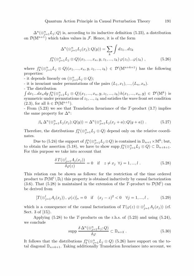
Quantum Action Principle in Causal Perturbation Theory 191
Δn(⊗nj=1Lj ;Q) is, according to its inductive definition (5.23), a distribution
on D(Mn+1) which takes values in F . Hence, it is of the form
Δn(⊗nj=1Lj(xj);Q(y)) =
∑k
∫dz1...dzk
fnk (⊗n
j=1Lj ⊗Q)(x1, ..., xn, y, z1, ..., zk)ϕ(z1)...ϕ(zk) , (5.26)
where fnk (⊗n
j=1Lj ⊗ Q)(x1, ..., xn, y, z1, ..., zk) ∈ D′(Mn+k+1) has the followingproperties:- it depends linearly on (⊗n
j=1Lj ⊗Q);- it is invariant under permutations of the pairs (L1, x1), ..., (Ln, xn).- The distribution∫dx1...dxndy f
nk (⊗n
j=1Lj ⊗ Q)(x1, ..., xn, y, z1, ..., zk)h(x1, ..., xn, y) ∈ D′(Mk) issymmetric under permutations of z1, ..., zk and satisfies the wave front set condition(2.3), for all h ∈ D(Mn+1).- From (5.23) we see that Translation Invariance of the T -product (3.7) impliesthe same property for Δn:
βa Δn(⊗nj=1Lj(xj);Q(y)) = Δn(⊗n
j=1Lj(xj + a);Q(y + a)) . (5.27)
Therefore, the distributions fnk (⊗n
j=1Lj ⊗Q) depend only on the relative coordi-nates.
Due to (5.24) the support of fnk (⊗n
j=1Lj⊗Q) is contained in Dn+1×Mk; but,to obtain the assertion (5.18), we have to show supp fn
k (⊗nj=1Lj ⊗Q) ⊂ Dn+k+1.
For this purpose we take into account that
δ T (⊗lj=1Aj(xj))δϕ(z)
= 0 if z �= xj ∀j = 1, ..., l . (5.28)
This relation can be shown as follows: for the restriction of the time orderedproduct to D(Ml \Dl) this property is obtained inductively by causal factorization(3.6). That (5.28) is maintained in the extension of the T -product to D(Ml) canbe derived from
[T (⊗lj=1Aj(xj)) , ϕ(z)]� = 0 if (xj − z)2 < 0 ∀j = 1, ..., l , (5.29)
which is a consequence of the causal factorization of T (ϕ(z) ⊗ ⊗lj=1Aj(xj)) (cf.
Sect. 3 of [15]).Applying (5.28) to the T -products on the r.h.s. of (5.23) and using (5.24),
we conclude
suppδΔn(⊗n
j=1Lj;Q)δϕ
⊂ Dn+2 . (5.30)
It follows that the distributions fnk (⊗n
j=1Lj ⊗ Q) (5.26) have support on the to-tal diagonal Dn+k+1. Taking additionally Translation Invariance into account, we

192 Ferdinand Brennecke and Michael Dutsch
conclude that these distributions are of the form
fnk (⊗n
j=1Lj ⊗Q)(x1, ..., xn, y, z1, ..., zk) =∑a,b
Ca,b(⊗nj=1Lj ⊗Q)
∂aδ(x1 − y, ..., xn − y) ∂bδ(z1 − y, ..., zk − y) , (5.31)
where the coefficients Ca,b(⊗nj=1Lj⊗Q) ∈ C depend linearly on (⊗n
j=1Lj⊗Q) andare symmetric in the first n factors. Inserting (5.31) into (5.26) we obtain (5.18),the corresponding maps Pn
a having the asserted properties.The important property (iii) is obtained by taking the classical limit � → 0
of the anomalous MWI (5.16): using (4.10) it results lim�→0 Δ(L;Q)(g; y) = 0.(b) The statement (5.19) is a modified version of Proposition 10(ii) in [6]. It
follows from the formulas ([6]-5.32-33) and ([6]-5.46-47) of that paper. Namely, byusing the causal Wick expansion of Δn (which follows from the Field Independenceof the T -product) and (5.24) it is derived in ([6]-5.32-33) that Δn is of the form
Δn(⊗nj=1Lj(xj);Q(y)) =
∑l,a,b
Cla,b (∂bδ)(x1 − y, ..., xn − y)
·n∏
i=1
li∏ji=1
(∂aijiϕ(xi)
)·
l∏j=1
∂ajϕ(y)
=∑l,a,b
∑d≤b
Cla,b,d (∂dδ)(x1 − y, ..., xn − y)
·n∏
i=1
(∂bi−di
li∏ji=1
(∂aijiϕ(y)
))·
l∏j=1
∂ajϕ(y) , (5.32)
where l ≡ (l1, ..., ln; l), a ≡ (a11, ..., a1l1 , ..., an1, ..., anln ; a1...al) and Cla,b , C
la,b,d
are numerical coefficients which depend also on (L1, ..., Ln, Q). Since the T -productsatisfies the axiom Scaling Degree the range of b is bounded by ([6]-5.46). Thel.h.s. of (5.19) is given by
|d|+ |b− d|+n∑
i=1
li∑ji=1
(|aiji |+
d− 22
)+
l∑j=1
(|aj|+
d− 22
), (5.33)
which agrees with the l.h.s. of ([6]-5.47). Hence, it is bounded by the r.h.s. of([6]-5.47). �
Remark 5.3. Since the T -product T (F⊗n) depends only on the (local) functionalF and not on how F is written as F =
∑k
∫dx gk(x)Pk(x) (gk ∈ D(M), Pk ∈ P),
we conclude from (5.23) that we may express the violating term Δ(L;Q)(g; y) asfollows: given A =
∫dxh(x)Q(x) δS0/δϕ(x) (h ∈ D(M), Q ∈ P), there exists a
linear and symmetric map ΔA : TFloc → Floc which is uniquely determined by
ΔA(eL(g)⊗ ) def=
∫dy h(y)Δ(L;Q)(g; y) . (5.34)
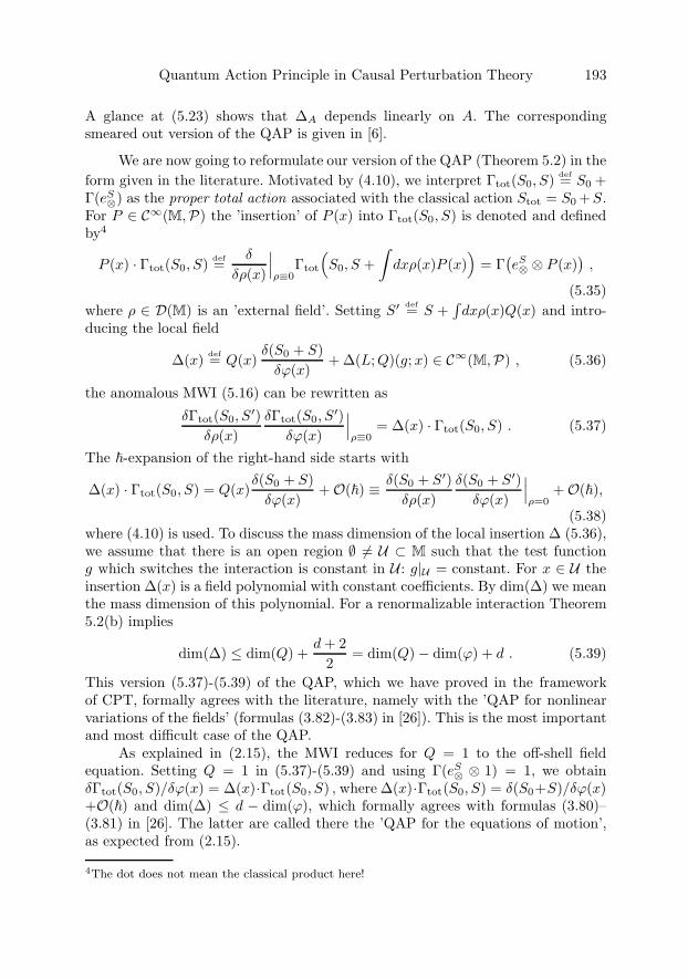
Quantum Action Principle in Causal Perturbation Theory 193
A glance at (5.23) shows that ΔA depends linearly on A. The correspondingsmeared out version of the QAP is given in [6].
We are now going to reformulate our version of the QAP (Theorem 5.2) in theform given in the literature. Motivated by (4.10), we interpret Γtot(S0, S) def= S0 +Γ(eS
⊗) as the proper total action associated with the classical action Stot = S0 +S.For P ∈ C∞(M,P) the ’insertion’ of P (x) into Γtot(S0, S) is denoted and definedby4
P (x) · Γtot(S0, S) def=δ
δρ(x)
∣∣∣ρ≡0
Γtot
(S0, S +
∫dxρ(x)P (x)
)= Γ
(eS⊗ ⊗ P (x)
),
(5.35)where ρ ∈ D(M) is an ’external field’. Setting S′ def= S +
∫dxρ(x)Q(x) and intro-
ducing the local field
Δ(x) def= Q(x)δ(S0 + S)δϕ(x)
+ Δ(L;Q)(g;x) ∈ C∞(M,P) , (5.36)
the anomalous MWI (5.16) can be rewritten as
δΓtot(S0, S′)
δρ(x)δΓtot(S0, S
′)δϕ(x)
∣∣∣ρ≡0
= Δ(x) · Γtot(S0, S) . (5.37)
The �-expansion of the right-hand side starts with
Δ(x) · Γtot(S0, S) = Q(x)δ(S0 + S)δϕ(x)
+O(�) ≡ δ(S0 + S′)δρ(x)
δ(S0 + S′)δϕ(x)
∣∣∣ρ=0
+O(�),
(5.38)where (4.10) is used. To discuss the mass dimension of the local insertion Δ (5.36),we assume that there is an open region ∅ �= U ⊂ M such that the test functiong which switches the interaction is constant in U : g|U = constant. For x ∈ U theinsertion Δ(x) is a field polynomial with constant coefficients. By dim(Δ) we meanthe mass dimension of this polynomial. For a renormalizable interaction Theorem5.2(b) implies
dim(Δ) ≤ dim(Q) +d + 2
2= dim(Q)− dim(ϕ) + d . (5.39)
This version (5.37)-(5.39) of the QAP, which we have proved in the frameworkof CPT, formally agrees with the literature, namely with the ’QAP for nonlinearvariations of the fields’ (formulas (3.82)-(3.83) in [26]). This is the most importantand most difficult case of the QAP.
As explained in (2.15), the MWI reduces for Q = 1 to the off-shell fieldequation. Setting Q = 1 in (5.37)-(5.39) and using Γ(eS
⊗ ⊗ 1) = 1, we obtainδΓtot(S0, S)/δϕ(x) = Δ(x)·Γtot(S0, S) , where Δ(x)·Γtot(S0, S) = δ(S0+S)/δϕ(x)+O(�) and dim(Δ) ≤ d − dim(ϕ), which formally agrees with formulas (3.80)–(3.81) in [26]. The latter are called there the ’QAP for the equations of motion’,as expected from (2.15).
4The dot does not mean the classical product here!

194 Ferdinand Brennecke and Michael Dutsch
Remark 5.4. An ’insertion’ (5.35) being a rather technical notion, the violatingterm Γ
(eS⊗ ⊗ Δ(L;Q)(g; y)
)in the anomalous MWI (5.16) can be much better
interpreted by writing (5.16) in terms of R-products:
R(eS⊗⊗Q(y)
δ(S0 + S)δϕ(y)
)+R(eS
⊗⊗Δ(L;Q)(g; y)) = R(eS⊗⊗Q(y))
δS0
δϕ(y). (5.40)
In this form, the violating term R(eS⊗ ⊗ Δ(L;Q)(g; y)) is the interacting field tothe interaction S and belonging to the local field Δ(L;Q)(g; y).
6. Algebraic renormalization
In this section we sketch, for the non-expert reader, the crucial role of the QAP inalgebraic renormalization. For shortness, we strongly simplify.
In algebraic renormalization one investigates, whether violations of Wardidentities can be removed by finite renormalizations of the T -products. The resultsabout the structure of the violating term given by the QAP are used as follows.• Algebraic renormalization starts with the anomalous MWI (5.16), that is the
result that the MWI can be violated only by an insertion term, i.e. a term ofthe form Γ
(eS⊗ ⊗Δ
)for some Δ ∈ Floc, cf. (5.40).
• Algebraic renormalization proceeds by induction on the order of �. To startthe induction one uses that Δ ≡ Δ(L;Q)(g; y) is of order O(�).
• Because the finite renormalization terms, which one may add to a T -product,must be local (in the strong sense of (5.18)) and compatible with the axiomScaling Degree, it is of crucial importance that Δ(L;Q)(g; y) satisfies locality(5.18) and the bound (5.19) on its mass dimension.
For many Ward identities it is possible to derive a consistency equation forΔ(L;Q)(g; y). Frequently this equation can be interpreted as the statement thatΔ(L;Q)(g; y) is a cocycle in the cohomology generated by the corresponding sym-metry transformation δ acting on some space K ⊂ Floc. For example, δ is anilpotent derivation (as the BRST-transformation5) or a family of derivations(δa)a=1,...,N fulfilling a Lie algebra relation [δa, δb] = fabc δc.
If the cocycle Δ(L;Q)(g; y) is a coboundary, it is usually possible to removethis violating term by a finite renormalization. Hence, in this case, the solvabilityof the considered Ward identity amounts to the question whether this cohomologyis trivial. For a renormalizable interaction the bound (5.19) on the mass dimensionmakes it possible to reduce the space K to a finite dimensional space, this simplifiesthe cohomological question enormously.
Many examples for this pattern are given in [26]. In the framework of CPTthe QAP and its application in algebraic renormalization have been used to provethe Ward identities of the O(N) scalar field model [6] (as a simple example to
5The cohomological structure of BRST-symmetry is much richer as mentioned here, see [17].
Quantum Action Principle in Causal Perturbation Theory 195
illustrate how algebraic renormalization works in CPT) and, much more relevant,BRST-symmetry of Yang-Mills fields in curved space-times [20].
Acknowledgement
We very much profitted from discussions with Klaus Fredenhagen. We are gratefulalso to Raymond Stora for valuable and detailed comments. While writing thispaper, M.D. was a guest of the Institute for Theoretical Physics of the Universityof Gottingen, he thanks for hospitality.
References
[1] G. Barnich, F. Brandt and M. Henneaux, Local BRST cohomology in gauge theories.Phys. Rept. 338 (2000), 439–569.
[2] C. Becchi, A. Rouet and R. Stora, Renormalization of the abelian Higgs-Kibble Model.Commun. Math. Phys. 42 (1975), 127–162
[3] C. Becchi, A. Rouet and R. Stora, Renormalization of gauge theories. Annals Phys.98 (1976), 287–321.
[4] N.N. Bogoliubov and D. V. Shirkov, Introduction to the Theory of Quantized Fields.Interscience Publishers, Inc., New York (1959)
[5] P. Breitenlohner and D. Maison, Dimensional renormalization and the action princi-ple. Commun. Math. Phys. 52 (1977), 11–38
[6] F. Brennecke and M. Dutsch, Removal of violations of the Master Ward Identity inperturbative QFT. Rev. Math. Phys. ... (2008), 100–120.
[7] R. Brunetti, M. Dutsch and K. Fredenhagen, Retarded products versus time-orderedproducts: a geometrical interpretation, work in preparation
[8] R. Brunetti and K. Fredenhagen, Microlocal analysis and interacting quantum fieldtheories: Renormalization on physical backgrounds. Commun. Math. Phys. 208 (2000),623–661
[9] M. Dutsch and F.-M. Boas, The Master Ward identity. Rev. Math. Phys. 14 (2002),977–1049.
[10] M. Dutsch and K. Fredenhagen, A local (perturbative) construction of observables ingauge theories: The example of QED. Commun. Math. Phys. 203 (1999), 71–105.
[11] M. Dutsch and K. Fredenhagen, Algebraic quantum field theory, perturbation theory,and the loop expansion. Commun. Math. Phys. 219 (2001), 5–30.
[12] M. Dutsch and K. Fredenhagen, Perturbative algebraic field theory, and deformationquantization. Fields Institute Communications 30 (2001), 151–160
[13] M. Dutsch and K. Fredenhagen, The Master Ward identity and generalizedSchwinger-Dyson equation in classical field theory. Commun. Math. Phys. 243 (2003),275–314.
[14] M. Dutsch and K. Fredenhagen, Causal perturbation theory in terms of retardedproducts, and a proof of the Action Ward identity. Rev. Math. Phys. 16 (2004), 1291–1348.
[15] H. Epstein and V. Glaser, The role of locality in perturbation theory. Ann. Inst. H.Poincare A19 (1973), 211.
196 Ferdinand Brennecke and Michael Dutsch
[16] R. Haag, Local Quantum Physics: Fields, Particles and Algebras. 2nd edn., Springer-Verlag, (1996)
[17] M. Henneaux and C. Teitelboim, Quantization of gauge systems. Princeton Univer-sity Press, Princeton, New Jersey (1992), 1–520.
[18] S. Hollands and R.M. Wald, Existence of local covariant time-ordered products ofquantum fields in curved spacetimes. Commun. Math. Phys. 231 (2002), 309–345
[19] S. Hollands and R.M. Wald, Conservation of the stress tensor in interacting quantumfield theory in curved spacetimes. Rev. Math. Phys. 17 (2005), 227–312
[20] S. Hollands, Renormalized Quantum Yang-Mills Fields in Curved Spacetime. gr-qc/0705.3340 (2007)
[21] G. Jona-Lasinio, Relativistic Field Theories with Symmetry-Breaking Solutions.Nuovo Cimento 34 (1964), 1790–1795
[22] Y.-M. P. Lam, Perturbation Lagrangian theory for scalar fields: Ward-Takahasi iden-tity and current algebra. Phys. Rev. D6 (1972), 2145–2161
[23] J. H. Lowenstein, Differential vertex operations in Lagrangian field theory. Commun.Math. Phys. 24 (1971), 1–21
[24] R.E. Peierls, The commutation laws of relativistic field theory. Proc. Roy. Soc. (Lon-don) A214 (1952), 143.
[25] O. Piguet and A. Rouet,Symmetries in perturbtaive quantum field theory. Phys. Rept.76 (1981), 1–77
[26] O. Piguet and S. P. Sorella, Algebraic renormalization: Perturbative renormalization,symmetries and anomalies. Lect. Notes Phys. M28 (1995), 1–134.
[27] G. Pinter, The Action Principle in Epstein Glaser Renormalization and Renormal-ization of the S Matrix of φ4-Theory. hep-th/9911063
[28] O. Steinmann, Perturbative Expansion in axiomatic field theory. Lect. Notes Phys.11 (1971)
[29] R. Stora, Pedagogical Experiments in Renormalized Perturbation Theory. Contri-bution to Conference ’Theory of Renormalization and Regularization’, Hesselberg,Germany, http://wwwthep.physik.uni-mainz.de/∼scheck (2002)
[30] R. Stora, The Wess Zumino consistency condition: a paradigm in renormalized per-turbation theory. Fortsch. Phys. 54 (2006), 175–182
[31] I. V. Tyutin, Gauge invariance in field theory and statistical physics in operatorformalism. LEBEDEV-75-39
[32] W. Zimmermann, Commun. Math. Phys. 15 (1969), 208
Ferdinand BrenneckeInstitut fur QuantenelektronikETH ZurichCH–8093 Zuriche-mail: [email protected]
Michael DutschInstitut fur Theoretische PhysikUniversitat ZurichCH–8057 Zuriche-mail: [email protected]

Quantum Field TheoryB. Fauser, J. Tolksdorf and E. Zeidler, Eds., 197–216c© 2009 Birkhauser Verlag Basel/Switzerland
Plane Wave Geometry and Quantum Physics
Matthias Blau
Abstract. I explain how the Lewis–Riesenfeld exact treatment of the time-dependent quantum harmonic oscillator can be understood in terms of thegeodesics and isometries of a plane wave metric, and I show how a curiousequivalence between two classes of Yang-Mills actions can be traced back tothe transformation relating plane waves in Rosen and Brinkmann coordinates.
Mathematics Subject Classification (2000). Primary 81T30; Secondary 83E30;81T13; 83C35.
Keywords. Rosen and Brinkmann coordinates, plane wave metric, gravita-tional waves, matrix string theory, harmonic oscillator, Yang-Mills theory,Heisenberg isometry algebra, duality in string theory.
1. Introduction
The characteristic interplay of geometry and gauge theory in string theory has ledto many new and exciting developments in recent years, in particular to progressin the understanding of certain strongly coupled quantum field theories. However,since string theorists were (regrettably) absent from the list of speakers at thisconference dedicated to recent developments in quantum field theory, I decidedto talk about a subject on the interface of geometry and quantum physics that isonly loosely inspired by, and not strictly dependent upon, string theory.1
Thus, as an embryonic example of the interplay between geometry and quan-tum physics in string theory (an example that requires neither knowledge norappreciation of string theory, but also does not do justice to the depth and rich-ness of these ideas in the string theory context), I will explain the relation between
This work has been supported by the Swiss National Science Foundation and by the EU undercontract MRTN-CT-2004-005104.1In retrospect this was a wise choice, because of the hostile attitude towards string theory atthis, in all other respects very charming and enjoyable, meeting, expressed in particular by someof the members of the senior pontificating classes.

198 Matthias Blau
some geometric properties of plane wave space-time metrics on the one hand andsome corresponding statements about quantum (gauge) theories on the other.
In section 2, I briefly review some of the basic and entertaining features ofthe geometry of plane wave metrics. In particular, I emphasize the ubiquitous andmultifaceted role of the time-dependent harmonic oscillator in this context, whichappears in the geodesic equations, in the description of the Heisenberg isometryalgebra of plane wave metrics, and in the coordinate transformation between thetwo standard (Rosen and Brinkmann) coordinate systems for these metrics.
The first application I will discuss is then naturally to the quantum theoryof time-dependent harmonic oscillators (section 3). In general one can quantizethese systems exactly using the powerful Lewis–Riesenfeld method of invariants.Embedding the problem of a time-dependent harmonic oscillator into the planewave setting equips it with a rich geometric structure, and links the dynamics ofthe harmonic oscillator to the conserved charges associated with the isometries. Iwill show that this provides a natural geometric explanation of the entire Lewis–Riesenfeld procedure.
As a second application, I will discuss a curious equivalence between two apriori apparently quite different classes of Yang-Mills theories (section 4). Onceagain, it is the plane wave perspective which provides an explanation for this.Namely, I will show that this equivalence can be traced back to the coordinatetransformation relating plane waves in Rosen and Brinkmann coordinates, andI add a few comments on what is the string theory context for these particularYang-Mills actions.
Section 2 is extracted (and adapted to present purposes) from my unpublishedlecture notes on plane waves and Penrose limits [1]. The material in section 3 isbased on [2], and section 4 is based on currently unpublished material that willappear in [3].
2. A brief introduction to the geometry of plane wave metrics
2.1. Plane waves in Rosen and Brinkmann coordinates: heuristics
Usually gravitational plane wave solutions of general relativity are discussed inthe context of the linearized theory. There one makes the Ansatz that the metrictakes the form
gμν = ημν + hμν (1)
where hμν is treated as a small perturbation of the Minkowski background met-ric ημν . To linear order in hμν , the Einstein equations (necessarily) reduce to awave equation. One finds that gravitational waves are transversally polarized. Forexample, a wave traveling in the (t, z)-direction distorts the metric only in thetransverse directions, and a typical solution of the linearized Einstein equations is
ds2 = −dt2 + dz2 + (δij + hij(z − t))dyidyj . (2)
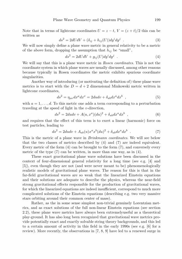
Plane Wave Geometry and Quantum Physics 199
Note that in terms of lightcone coordinates U = z − t, V = (z + t)/2 this can bewritten as
ds2 = 2dUdV + (δij + hij(U))dyidyj . (3)We will now simply define a plane wave metric in general relativity to be a metricof the above form, dropping the assumption that hij be “small”,
ds2 = 2dUdV + gij(U)dyidyj . (4)
We will say that this is a plane wave metric in Rosen coordinates. This is not thecoordinate system in which plane waves are usually discussed, among other reasonsbecause typically in Rosen coordinates the metric exhibits spurious coordinatesingularities.
Another way of introducing (or motivating the definition of) these plane wavemetrics is to start with the D = d + 2 dimensional Minkowski metric written inlightcone coordinates,
ds2 = ημνdxμdxν = 2dudv + δabdx
adxb , (5)
with a = 1, . . . , d. To this metric one adds a term corresponding to a perturbationtraveling at the speed of light in the v-direction,
ds2 = 2dudv + A(u, xa)(du)2 + δabdxadxb , (6)
and requires that the effect of this term is to exert a linear (harmonic) force ontest particles, leading to
ds2 = 2dudv + Aab(u)xaxb(du)2 + δabdxadxb . (7)
This is the metric of a plane wave in Brinkmann coordinates. We will see belowthat the two classes of metrics described by (4) and (7) are indeed equivalent.Every metric of the form (4) can be brought to the form (7), and conversely everymetric of the type (7) can be written, in more than one way, as in (4).
These exact gravitational plane wave solutions have been discussed in thecontext of four-dimensional general relativity for a long time (see e.g. [4] and[5]), even though they are not (and were never meant to be) phenomenologicallyrealistic models of gravitational plane waves. The reason for this is that in thefar-field gravitational waves are so weak that the linearized Einstein equationsand their solutions are adequate to describe the physics, whereas the near-fieldstrong gravitational effects responsible for the production of gravitational waves,for which the linearized equations are indeed insufficient, correspond to much morecomplicated solutions of the Einstein equations (describing e.g. two very massivestars orbiting around their common center of mass).
Rather, as the in some sense simplest non-trivial genuinely Lorentzian met-rics, and as exact solutions of the full non-linear Einstein equations (see section2.2), these plane wave metrics have always been extremelyuseful as a theoreticalplay-ground. It has also long been recognized that gravitational wave metrics pro-vide potentially exact and exactly solvable string theory backgrounds, and this ledto a certain amount of activity in this field in the early 1990s (see e.g. [6] for areview). More recently, the observations in [7, 8, 9] have led to a renewed surge in
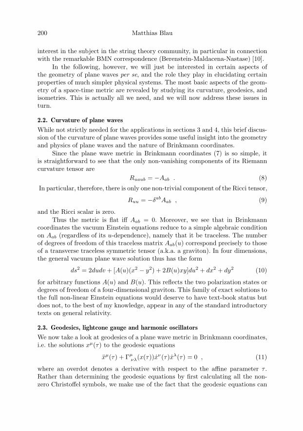
200 Matthias Blau
interest in the subject in the string theory community, in particular in connectionwith the remarkable BMN correspondence (Berenstein-Maldacena-Nastase) [10].
In the following, however, we will just be interested in certain aspects ofthe geometry of plane waves per se, and the role they play in elucidating certainproperties of much simpler physical systems. The most basic aspects of the geom-etry of a space-time metric are revealed by studying its curvature, geodesics, andisometries. This is actually all we need, and we will now address these issues inturn.
2.2. Curvature of plane waves
While not strictly needed for the applications in sections 3 and 4, this brief discus-sion of the curvature of plane waves provides some useful insight into the geometryand physics of plane waves and the nature of Brinkmann coordinates.
Since the plane wave metric in Brinkmann coordinates (7) is so simple, itis straightforward to see that the only non-vanishing components of its Riemanncurvature tensor are
Ruaub = −Aab . (8)
In particular, therefore, there is only one non-trivial component of the Ricci tensor,
Ruu = −δabAab , (9)
and the Ricci scalar is zero.Thus the metric is flat iff Aab = 0. Moreover, we see that in Brinkmann
coordinates the vacuum Einstein equations reduce to a simple algebraic conditionon Aab (regardless of its u-dependence), namely that it be traceless. The numberof degrees of freedom of this traceless matrix Aab(u) correspond precisely to thoseof a transverse traceless symmetric tensor (a.k.a. a graviton). In four dimensions,the general vacuum plane wave solution thus has the form
ds2 = 2dudv + [A(u)(x2 − y2) + 2B(u)xy]du2 + dx2 + dy2 (10)
for arbitrary functions A(u) and B(u). This reflects the two polarization states ordegrees of freedom of a four-dimensional graviton. This family of exact solutions tothe full non-linear Einstein equations would deserve to have text-book status butdoes not, to the best of my knowledge, appear in any of the standard introductorytexts on general relativity.
2.3. Geodesics, lightcone gauge and harmonic oscillators
We now take a look at geodesics of a plane wave metric in Brinkmann coordinates,i.e. the solutions xμ(τ) to the geodesic equations
xμ(τ) + Γμνλ(x(τ))xν (τ)xλ(τ) = 0 , (11)
where an overdot denotes a derivative with respect to the affine parameter τ .Rather than determining the geodesic equations by first calculating all the non-zero Christoffel symbols, we make use of the fact that the geodesic equations can

Plane Wave Geometry and Quantum Physics 201
be obtained more efficiently, and in a way that allows us to directly make use ofthe symmetries of the problem, as the Euler-Lagrange equations of the Lagrangian
L = 12gμν x
μxν
= uv + 12Aab(u)xaxbu2 + 1
2 �x2 , (12)
supplemented by the constraint 2L = ε, where ε = 0 (ε = −1) for massless(massive) particles. Since nothing depends on v, the lightcone momentum
pv =∂L∂v
= u (13)
is conserved. For pv = 0, the particle obviously does not feel the curvature termAab, and the geodesics are straight lines. When pv �= 0, one has u = pvτ + u0, andby an affine transformation of τ one can always choose the lightcone gauge
u = τ . (14)
Then the geodesic equations for the transverse coordinates are the Euler-Lagrangeequations
xa(τ) = Aab(τ)xb(τ) . (15)These are the equation of motion of a non-relativistic harmonic oscillator with(possibly time-dependent) frequency matrix ω2
ab(τ) = −Aab(τ). The constraint2L = ε, or
2v(τ) + Aab(τ)xa(τ)xb(τ) + δabxa(τ)xb(τ) = ε, (16)
is then a first integral of the equation of motion for the remaining coordinate v(τ),and is readily integrated to give v(τ) in terms of the solutions to the harmonicoscillator equation for xa(τ).
By definition the lightcone Hamiltonian is (minus!) the momentum pu con-jugate to u (in the lightcone gauge u = τ),
Hlc = −pu . (17)
Usingpu = guμx
μ = v + Aab(τ)xaxb (18)and the constraint, one finds that the lightcone Hamiltonian is just (for ε �= 0 upto an irrelevant constant) the Hamiltonian of the above harmonic oscillator,
Hlc = 12 (δabx
axb −Aab(τ)xaxb)− 12ε ≡ Hho − 1
2ε . (19)
Note also that, in the lightcone gauge, the complete relativistic particle Lagrangian
L = v + 12Aab(τ)xaxb + 1
2 �x2 = Lho + v (20)
differs from the harmonic oscillator Lagrangian only by a total time-derivative.In summary, we note that in the lightcone gauge the equations of motion of
a relativistic particle in the plane wave metric reduce to those of a non-relativisticharmonic oscillator. This harmonic oscillator equation plays a central role in thefollowing and will reappear several times below in different contexts, e.g. whendiscussing the transformation from Rosen to Brinkmann coordinates, or whenanalyzing the isometries of a plane wave metric.
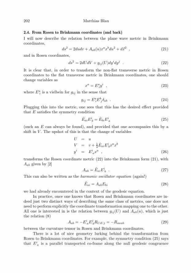
202 Matthias Blau
2.4. From Rosen to Brinkmann coordinates (and back)
I will now describe the relation between the plane wave metric in Brinkmanncoordinates,
ds2 = 2dudv + Aab(u)xaxbdu2 + d�x2 , (21)
and in Rosen coordinates,
ds2 = 2dUdV + gij(U)dyidyj . (22)
It is clear that, in order to transform the non-flat transverse metric in Rosencoordinates to the flat transverse metric in Brinkmann coordinates, one shouldchange variables as
xa = Eaiy
i , (23)
where Eai is a vielbein for gij in the sense that
gij = EaiE
bjδab . (24)
Plugging this into the metric, one sees that this has the desired effect providedthat E satisfies the symmetry condition
EaiEib = EbiE
ia (25)
(such an E can always be found), and provided that one accompanies this by ashift in V . The upshot of this is that the change of variables
U = u
V = v + 12 EaiE
ibx
axb
yi = Eiax
a , (26)
transforms the Rosen coordinate metric (22) into the Brinkmann form (21), withAab given by [2]
Aab = EaiEib . (27)
This can also be written as the harmonic oscillator equation (again!)
Eai = AabEbi (28)
we had already encountered in the context of the geodesic equation.In practice, once one knows that Rosen and Brinkmann coordinates are in-
deed just two distinct ways of describing the same class of metrics, one does notneed to perform explicitly the coordinate transformation mapping one to the other.All one is interested in is the relation between gij(U) and Aab(u), which is justthe relation (8)
Aab = −EiaE
jbRUiUj = −Ruaub (29)
between the curvature tensor in Rosen and Brinkmann coordinates.There is a lot of nice geometry lurking behind the transformation from
Rosen to Brinkmann coordinates. For example, the symmetry condition (25) saysthat Ei
a is a parallel transported co-frame along the null geodesic congruence
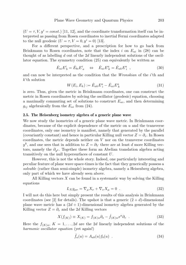
Plane Wave Geometry and Quantum Physics 203
(U = τ, V, yi = const.) [11, 12], and the coordinate transformation itself can be in-terpreted as passing from Rosen coordinates to inertial Fermi coordinates adaptedto the null geodesic (U = τ, V = 0, yi = 0) [13].
For a different perspective, and a prescription for how to go back fromBrinkmann to Rosen coordinates, note that the index i on Eai in (28) can bethought of as labelling d out of the 2d linearly independent solutions of the oscil-lator equation. The symmetry condition (25) can equivalently be written as
EaiEib = EbiE
ia ⇔ EaiE
ak = EakE
ai , (30)
and can now be interpreted as the condition that the Wronskian of the i’th andk’th solution
W (Ei, Ek) := EakEai − EaiE
ak (31)
is zero. Thus, given the metric in Brinkmann coordinates, one can construct themetric in Rosen coordinates by solving the oscillator (geodesic) equation, choosinga maximally commuting set of solutions to construct Eai, and then determininggij algebraically from the Eai from (24).
2.5. The Heisenberg isometry algebra of a generic plane wave
We now study the isometries of a generic plane wave metric. In Brinkmann coor-dinates, because of the explicit dependence of the metric on u and the transversecoordinates, only one isometry is manifest, namely that generated by the parallel(covariantly constant) and hence in particular Killing null vector Z = ∂v. In Rosencoordinates, the metric depends neither on V nor on the transverse coordinatesyk, and one sees that in addition to Z = ∂V there are at least d more Killing vec-tors, namely the ∂yk . Together these form an Abelian translation algebra actingtransitively on the null hypersurfaces of constant U .
However, this is not the whole story. Indeed, one particularly interesting andpeculiar feature of plane wave space-times is the fact that they generically possess asolvable (rather than semi-simple) isometry algebra, namely a Heisenberg algebra,only part of which we have already seen above.
All Killing vectors X can be found in a systematic way by solving the Killingequations
LXgμν = ∇μXν +∇νXμ = 0 . (32)
I will not do this here but simply present the results of this analysis in Brinkmanncoordinates (see [2] for details). The upshot is that a generic (2 + d)-dimensionalplane wave metric has a (2d + 1)-dimensional isometry algebra generated by theKilling vector Z = ∂v and the 2d Killing vectors
X(f(K)) ≡ X(K) = f(K)a∂a − f(K)axa∂v . (33)
Here the f(K)a, K = 1, . . . , 2d are the 2d linearly independent solutions of theharmonic oscillator equation (yet again!)
fa(u) = Aab(u)fb(u) . (34)

204 Matthias Blau
These Killing vectors satisfy the algebra
[X(J), X(K)] = −W (f(J), f(K))Z (35)[X(J), Z] = 0 , (36)
where the Wronskian W (f(J), f(K)) is, exactly as in (31), given by
W (f(J), f(K)) =∑
a
(f(J)af(K)a − f(K)af(J)a) . (37)
It is of course constant (independent of u) as a consequence of the harmonicoscillator equation. This is already the Heisenberg algebra. To make this moreexplicit, one can make a convenient choice of basis for the solutions f(J) by splittingthe f(J) into two sets of solutions
{f(J)} → {q(a), p(a)} (38)
characterized by the initial conditions
q(a)b(u0) = δab q(a)b(u0) = 0p(a)b(u0) = 0 p(a)b(u0) = δab . (39)
Since the Wronskian of these functions is independent of u, it can be determinedby evaluating it at u = u0. Then one can immediately read off that
W (q(a), q(b)) = W (p(a), p(b)) = 0W (q(a), p(b)) = δab . (40)
Therefore the corresponding Killing vectors
Q(a) = X(q(a)) , P(a) = X(p(a)) (41)
and Z satisfy the canonically normalized Heisenberg algebra
[Q(a), Z] = [P(a), Z] = 0[Q(a), Q(b)] = [P(a), P(b)] = 0[Q(a), P(b)] = −δabZ . (42)
As we had noted before, in Rosen coordinates, the (d+1) translational isome-tries in the V and yk directions, generated by the Killing vectors Z = ∂V andQ(k) = ∂yk , are manifest. One can check that the “missing” d Killing vectors P(k)
are given by
P(k) = −yk∂V +∫ u
du′ gkm(u′)∂ym . (43)
It is straightforward to verify that together they also generate the Heisenbergalgebra (42).
These considerations also provide yet another perspective on the transfor-mation from Brinkmann to Rosen coordinates, and the vanishing Wronskian con-dition discussed at the end of section 2.4. Indeed, passing from Brinkmann toRosen coordinates can be interpreted as passing to coordinates in which half ofthe translational Heisenberg algebra symmetries are manifest. This is achieved by

Plane Wave Geometry and Quantum Physics 205
choosing the (transverse) coordinate lines to be the integral curves of these Killingvectors. This is of course only possible if these Killing vectors commute, i.e. theWronskian of the corresponding solutions of the harmonic oscillator equation iszero, and results in a metric which is independent of the transverse coordinates,namely the plane wave metric in Rosen coordinates.
2.6. Geodesics, isometries, and conserved charges
We can now combine the results of the previous sections to determine the conservedcharges carried by particles moving geodesically in the plane wave geometry. Ingeneral, given any Killing vector X , there is a corresponding conserved chargeC(X),
C(X) = gμνXμxμ . (44)
That C(X) is indeed constant along the trajectory of the geodesic xμ(τ) can easilybe verified by using the geodesic and Killing equations.
The conserved charge corresponding to the Killing vector Z = ∂v, the centralelement of the Heisenberg algebra, is, none too surprisingly, nothing other thanthe conserved lightcone momentum pv (13) of section 2.3,
C(Z) = gvμxμ = u = pv . (45)
In addition to Z, for any solution f of the harmonic oscillator equation we have aKilling vector X(f) (33),
X(f) = fa∂a − faxa∂v . (46)
The associated conserved charge is
C(X(f)) = fapa − fax
a . (47)
(here we have used the, now more appropriate, phase space notation pa = xa).This is rather trivially conserved (constant), since both fa and xa are solutions ofthe same ubiquitous harmonic oscillator equation and C(X(f)) is nothing otherthan their constant Wronskian,
C(X(f)) = W (f, x) . (48)
Thus these somewhat tautological conserved charges are not helpful in integratingthe geodesic or harmonic oscillator equations. Nevertheless, the very fact that theyexist, and that they satisfy a (Poisson bracket) Heisenberg algebra, will turn outto be conceptually important in section 3. We will denote the conserved chargescorresponding to the Killing vectors Q(a) and P(a) (41) by
C(Q(a)) ≡ Q(a) C(P(a)) ≡ P(a) . (49)
The Poisson brackets among the charges C(X(f)) can be determined from thecanonical Poisson brackets {xa, pb} = δab to be
{X(f1), X(f2)} = {f1apa − f1ax
a, f2apa − f2ax
a} = W (f1, f2) (50)
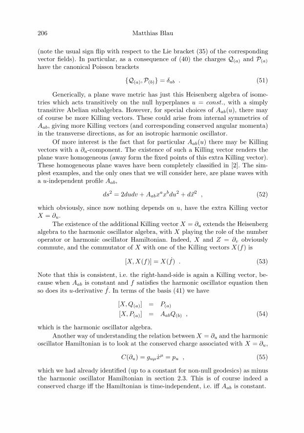
206 Matthias Blau
(note the usual sign flip with respect to the Lie bracket (35) of the correspondingvector fields). In particular, as a consequence of (40) the charges Q(a) and P(a)
have the canonical Poisson brackets
{Q(a),P(b)} = δab . (51)
Generically, a plane wave metric has just this Heisenberg algebra of isome-tries which acts transitively on the null hyperplanes u = const., with a simplytransitive Abelian subalgebra. However, for special choices of Aab(u), there mayof course be more Killing vectors. These could arise from internal symmetries ofAab, giving more Killing vectors (and corresponding conserved angular momenta)in the transverse directions, as for an isotropic harmonic oscillator.
Of more interest is the fact that for particular Aab(u) there may be Killingvectors with a ∂u-component. The existence of such a Killing vector renders theplane wave homogeneous (away form the fixed points of this extra Killing vector).These homogeneous plane waves have been completely classified in [2]. The sim-plest examples, and the only ones that we will consider here, are plane waves witha u-independent profile Aab,
ds2 = 2dudv + Aabxaxbdu2 + d�x2 , (52)
which obviously, since now nothing depends on u, have the extra Killing vectorX = ∂u.
The existence of the additional Killing vector X = ∂u extends the Heisenbergalgebra to the harmonic oscillator algebra, with X playing the role of the numberoperator or harmonic oscillator Hamiltonian. Indeed, X and Z = ∂v obviouslycommute, and the commutator of X with one of the Killing vectors X(f) is
[X,X(f)] = X(f) . (53)
Note that this is consistent, i.e. the right-hand-side is again a Killing vector, be-cause when Aab is constant and f satisfies the harmonic oscillator equation thenso does its u-derivative f . In terms of the basis (41) we have
[X,Q(a)] = P(a)
[X,P(a)] = AabQ(b) , (54)
which is the harmonic oscillator algebra.Another way of understanding the relation between X = ∂u and the harmonic
oscillator Hamiltonian is to look at the conserved charge associated with X = ∂u,
C(∂u) = guμxμ = pu , (55)
which we had already identified (up to a constant for non-null geodesics) as minusthe harmonic oscillator Hamiltonian in section 2.3. This is of course indeed aconserved charge iff the Hamiltonian is time-independent, i.e. iff Aab is constant.
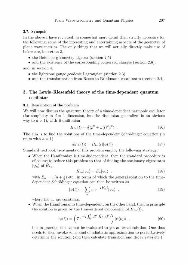
Plane Wave Geometry and Quantum Physics 207
2.7. Synopsis
In the above I have reviewed, in somewhat more detail than strictly necessary forthe following, some of the interesting and entertaining aspects of the geometry ofplane wave metrics. The only things that we will actually directly make use ofbelow are, in section 3,• the Heisenberg isometry algebra (section 2.5)• and the existence of the corresponding conserved charges (section 2.6),
and, in section 4,• the lightcone gauge geodesic Lagrangian (section 2.3)• and the transformation from Rosen to Brinkmann coordinates (section 2.4).
3. The Lewis–Riesenfeld theory of the time-dependent quantumoscillator
3.1. Description of the problem
We will now discuss the quantum theory of a time-dependent harmonic oscillator(for simplicity in d = 1 dimension, but the discussion generalizes in an obviousway to d > 1), with Hamiltonian
Hho(t) = 12 (p2 + ω(t)2x2) . (56)
The aim is to find the solutions of the time-dependent Schrodinger equation (inunits with � = 1)
i∂t|ψ(t)〉 = Hho(t)|ψ(t)〉 . (57)Standard textbook treatments of this problem employ the following strategy:• When the Hamiltonian is time-independent, then the standard procedure is
of course to reduce this problem to that of finding the stationary eigenstates|ψn〉 of Hho,
Hho|ψn〉 = En|ψn〉 , (58)with En = ω(n+ 1
2 ) etc., in terms of which the general solution to the time-dependent Schrodinger equation can then be written as
|ψ(t)〉 =∑
n
cne−iEnt|ψn〉 , (59)
where the cn are constants.• When the Hamiltonian is time-dependent, on the other hand, then in principle
the solution is given by the time-ordered exponential of Hho(t),
|ψ(t)〉 =(T e−i
∫ t
t0dt′ Hho(t′)
)|ψ(t0)〉 , (60)
but in practice this cannot be evaluated to get an exact solution. One thusneeds to then invoke some kind of adiabatic approximation to perturbativelydetermine the solution (and then calculate transition and decay rates etc.).
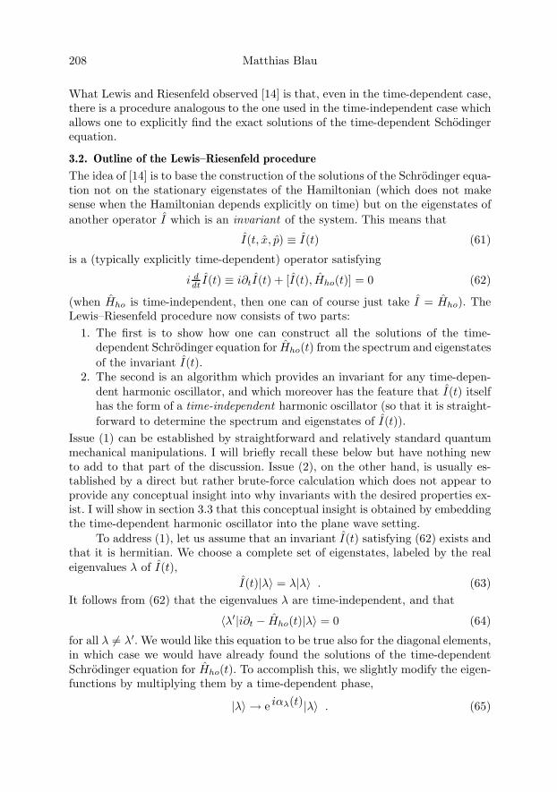
208 Matthias Blau
What Lewis and Riesenfeld observed [14] is that, even in the time-dependent case,there is a procedure analogous to the one used in the time-independent case whichallows one to explicitly find the exact solutions of the time-dependent Schodingerequation.
3.2. Outline of the Lewis–Riesenfeld procedure
The idea of [14] is to base the construction of the solutions of the Schrodinger equa-tion not on the stationary eigenstates of the Hamiltonian (which does not makesense when the Hamiltonian depends explicitly on time) but on the eigenstates ofanother operator I which is an invariant of the system. This means that
I(t, x, p) ≡ I(t) (61)
is a (typically explicitly time-dependent) operator satisfying
i ddt I(t) ≡ i∂tI(t) + [I(t), Hho(t)] = 0 (62)
(when Hho is time-independent, then one can of course just take I = Hho). TheLewis–Riesenfeld procedure now consists of two parts:
1. The first is to show how one can construct all the solutions of the time-dependent Schrodinger equation for Hho(t) from the spectrum and eigenstatesof the invariant I(t).
2. The second is an algorithm which provides an invariant for any time-depen-dent harmonic oscillator, and which moreover has the feature that I(t) itselfhas the form of a time-independent harmonic oscillator (so that it is straight-forward to determine the spectrum and eigenstates of I(t)).
Issue (1) can be established by straightforward and relatively standard quantummechanical manipulations. I will briefly recall these below but have nothing newto add to that part of the discussion. Issue (2), on the other hand, is usually es-tablished by a direct but rather brute-force calculation which does not appear toprovide any conceptual insight into why invariants with the desired properties ex-ist. I will show in section 3.3 that this conceptual insight is obtained by embeddingthe time-dependent harmonic oscillator into the plane wave setting.
To address (1), let us assume that an invariant I(t) satisfying (62) exists andthat it is hermitian. We choose a complete set of eigenstates, labeled by the realeigenvalues λ of I(t),
I(t)|λ〉 = λ|λ〉 . (63)It follows from (62) that the eigenvalues λ are time-independent, and that
〈λ′|i∂t − Hho(t)|λ〉 = 0 (64)
for all λ �= λ′. We would like this equation to be true also for the diagonal elements,in which case we would have already found the solutions of the time-dependentSchrodinger equation for Hho(t). To accomplish this, we slightly modify the eigen-functions by multiplying them by a time-dependent phase,
|λ〉 → e iαλ(t)|λ〉 . (65)
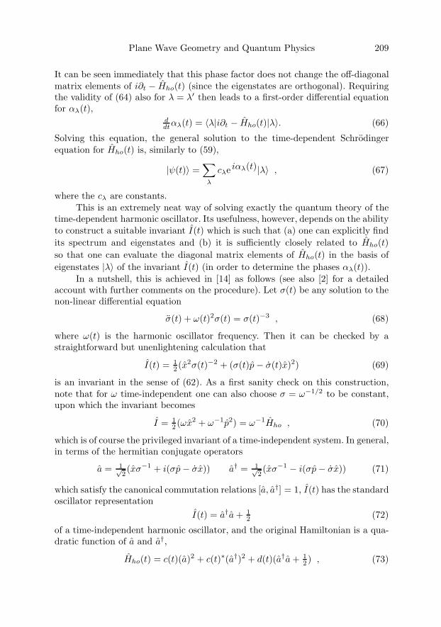
Plane Wave Geometry and Quantum Physics 209
It can be seen immediately that this phase factor does not change the off-diagonalmatrix elements of i∂t − Hho(t) (since the eigenstates are orthogonal). Requiringthe validity of (64) also for λ = λ′ then leads to a first-order differential equationfor αλ(t),
ddtαλ(t) = 〈λ|i∂t − Hho(t)|λ〉. (66)
Solving this equation, the general solution to the time-dependent Schrodingerequation for Hho(t) is, similarly to (59),
|ψ(t)〉 =∑
λ
cλe iαλ(t)|λ〉 , (67)
where the cλ are constants.This is an extremely neat way of solving exactly the quantum theory of the
time-dependent harmonic oscillator. Its usefulness, however, depends on the abilityto construct a suitable invariant I(t) which is such that (a) one can explicitly findits spectrum and eigenstates and (b) it is sufficiently closely related to Hho(t)so that one can evaluate the diagonal matrix elements of Hho(t) in the basis ofeigenstates |λ〉 of the invariant I(t) (in order to determine the phases αλ(t)).
In a nutshell, this is achieved in [14] as follows (see also [2] for a detailedaccount with further comments on the procedure). Let σ(t) be any solution to thenon-linear differential equation
σ(t) + ω(t)2σ(t) = σ(t)−3 , (68)
where ω(t) is the harmonic oscillator frequency. Then it can be checked by astraightforward but unenlightening calculation that
I(t) = 12 (x2σ(t)−2 + (σ(t)p− σ(t)x)2) (69)
is an invariant in the sense of (62). As a first sanity check on this construction,note that for ω time-independent one can also choose σ = ω−1/2 to be constant,upon which the invariant becomes
I = 12 (ωx2 + ω−1p2) = ω−1Hho , (70)
which is of course the privileged invariant of a time-independent system. In general,in terms of the hermitian conjugate operators
a = 1√2(xσ−1 + i(σp− σx)) a† = 1√
2(xσ−1 − i(σp− σx)) (71)
which satisfy the canonical commutation relations [a, a†] = 1, I(t) has the standardoscillator representation
I(t) = a†a + 12 (72)
of a time-independent harmonic oscillator, and the original Hamiltonian is a qua-dratic function of a and a†,
Hho(t) = c(t)(a)2 + c(t)∗(a†)2 + d(t)(a†a + 12 ) , (73)

210 Matthias Blau
where e.g. d(t) = 12 (ω(t)2σ(t)2 + σ(t)2 + σ(t)−2). This makes it straightforward
to evaluate e.g. the diagonal matrix elements of Hho(t) in the standard basis ofeigenstates of I(t).
Finally, the general solution to (68) can be written in terms of any two linearlyindependent solutions f1, f2 to the classical harmonic oscillator equation for Hho(t)(this is (68) with zero on the rhs instead of the non-linear term). Normalizing theirWronskian to 1, the general solution σ(t) is [14]
σ = ±[c21f
21 + c22f
22 ± 2(c21c
22 − 1)1/2f1f2
]1/2
, (74)
where ci are constants subject to the condition that the solution is real, and thesigns can be chosen independently.
3.3. Deducing the procedure from the plane wave geometry
While the procedure outlined above provides a concrete (and in practice also veryuseful) algorithm to solve exactly the quantum theory of a time-dependent har-monic oscillator (and certain other time-dependent systems [14]), it remains some-what unsatisfactory from a conceptual point of view. In particular, it is not clearfrom the construction
• why invariants with the desired properties exist in the first place;• why solutions to the classical equations play a role in the construction of
these quantum invariants;• why one should solve the non-linear equation (68) if, in any case, in the end it
all boils down to solutions of the ordinary linear classical harmonic oscillatorequation appearing in (74).
Here is where insight is gained by realizing the harmonic oscillator equation asthe geodesic equation in a plane wave metric. Recall that in section 2.5 we hadfound a Heisenberg isometry algebra which, in particular, includes the “hidden”symmetries generated by the Killing vector fields (33,46)
X(f) = fa∂a − faxa∂v , (75)
where f is a solution of the classical harmonic oscillator equation, and the corre-sponding “hidden” conserved charges (47)
C(X(f)) = fapa − fax
a . (76)
In particular, we had obtained the conserved charges Q(a) and P(a) (49). Theseare linear in the phase space variables xa and pa, and thus we can unambiguouslyassociate to them quantum operators
Q(a) → Q(a) P(a) → P(a) (77)
which, by construction, are invariants in the sense of (62),
ddtQ(a) = d
dt P(a) = 0 , (78)
Plane Wave Geometry and Quantum Physics 211
and which satisfy the canonical commutation relations (cf. (51))
[Q(a), P(b)] = iδab . (79)
Note that to “see” these invariants, one has to extend the harmonic oscillatorconfiguration space not just by the time-direction t = u, but one also has to addyet another dimension, the null direction v.
The rest is now straightforward. Since Q(a) and P(b) are invariants, also anyquadratic operator in these variables (with constant coefficients) is an invariant.In the one-dimensional case (d = 1), we can e.g. consider invariants of the form
I(t) = 12M P2 + MΩ2
2 Q2 , (80)
which we can write in terms of invariant creation and annihilation operators Aand A† (constructed in the usual way from Q and P) as
I(t) = Ω(A†A+ 12 ) . (81)
Let us now compare this in detail with the results of section 3.2. First of all, tomatch with the (arbitrary choice of) normalization of the invariant (72), we chooseΩ = 1. Next we can identify what σ(t)2 is by identifying it with the coefficient of p2
in the expansion of (80) in terms of p and x. The upshot is that σ(t) has preciselythe form given in (74), with c21 = 1 and c22 = 1/M . Finally, one sees that theinvariant oscillators A and A† are related to the oscillators a and a† by a unitarytransformation which is precisely the unitary transformation that implements thephase transformation (65) on the eigenstates of the invariant.
We have thus come full circle. Starting with the conserved charges associatedwith the Heisenberg algebra Killing vectors, we have constructed quadratic quan-tum invariants and have reproduced all the details of the Lewis–Riesenfeld algo-rithm, including the phase factors αλ(t). Constructing the Fock space in the usualway, one then obtains all the solutions (67) to the time-dependent Schrodingerequation.
4. A curious equivalence between two classes of Yang-Mills actions
4.1. Description of the problem
A prototypical non-Abelian Yang-Mills + scalar action in n = p+1 dimensions, ob-tained e.g. by the dimensional reduction of pure Yang-Mills theory (with standardLagrangian L ∼ trFMNFMN ) in D space-time dimensions down to n dimensions,has the form
SY M =∫
dnσTr(− 1
4g−2Y MηαγηβδFαβFγδ − 1
2ηαβDαφ
aDβφa + 1
4g2Y M [φa, φb]2
).
(82)Here the φa, a = 1, . . . , D−n, are hermitian scalar fields arising from the internalcomponents of the gauge field and thus taking values in the adjoint representation
212 Matthias Blau
of the gauge group, the covariant derivative is
Dαφa = ∂αφ
a − i[Aα, φa] , (83)
Aα is the gauge field, Fαβ its curvature, g2Y M denotes the Yang-Mills coupling
constant, Tr a Lie algebra trace, and in writing the above action I have suppressedall Lie algebra labels.
This basic action can of course be modified in various ways, e.g. by addingfurther fields (we will not do this), or by modifying the couplings of the scalarfields. We will consider two such modifications. The first one simply consists ofadding (possibly time-dependent) mass terms for the scalars. Denoting the scalarsin this model by Xa, the action reads
SBC =∫
dnσTr(− 1
4g−2Y MηαγηβδFαβFγδ − 1
2ηαβδabDαX
aDβXb
+ 14g
2Y Mδacδbd[Xa, Xb][Xc, Xd] + 1
2Aab(t)XaXb)
,
(84)
with Aab(t) minus the mass-squared matrix.The second class of actions arises from (82) by replacing the flat metric δab
on the scalar field space (suppressed in (82) but written out explicitly in (84)) bya time-dependent matrix gij(t) of “coupling constants”, but without adding anymass terms. Denoting the scalars in this model by Y i, the action reads
SRC =∫
dnσ Tr(− 1
4g−2Y MηαγηβδFαβFγδ − 1
2ηαβgij(t)DαY
iDβYj
+ 14g
2Y Mgik(t)gjl(t)[Y i, Y j ][Y k, Y l]
).
(85)
The reason for the subscripts BC and RC on the actions will, if not already obviousat this stage, become apparent below. In any case, the claim is now that these two,apparently rather different, classes of Yang-Mills actions are simply related by acertain linear field redefinition Y i = Ei
aXa of the scalar fields,
SRC [Aα, Yi = Ei
aXa] = SBC [Aα, X
a] . (86)
We could straightaway prove this by a brute-force calculation, but this wouldbe rather unenlightening. Instead, we will first consider a much simpler classicalmechanics toy model of this equivalence (section 4.2), and we will then be able toestablish (86) with hardly any calculation at all (section 4.3). At the end, I willbriefly indicate why one is led to consider actions of the type (84,85) in the firstplace, and why from that point of view one can a priori anticipate the validity ofan identity like (86).
4.2. A classical mechanics toy model
As a warm-up exercise, consider the standard harmonic oscillator Lagrangian (nowmysteriously labeled bc)
Lbc(x) = 12 (x2 − ω2x2) , (87)
and the (exotic) Lagrangian
Lrc(y) = 12 sin2 ωt y2 (88)

Plane Wave Geometry and Quantum Physics 213
with a time-dependent kinetic term. Now consider the transformation
y = (sinωt)−1x . (89)
Then one findsLrc(y) = 1
2 (x2 + ω2x2 cot2 ωt− 2ωxx cotωt)
= 12 (x2 − ω2x2)− d
dt (12ωx
2 cotωt)
= Lbc(x) + ddt (. . .)
(90)
Thus, up to a total time-derivative the linear transformation (89) transforms theexotic (and seemingly somewhat singular) Lagrangian (88) to the completely regu-lar “massive” Lagrangian (87), and the corresponding actions are essentially iden-tical. This should be thought of as the counterpart of the statement that the Rosencoordinate plane wave metric
ds2 = 2dUdV + sin2 ωU(dy)2 (91)
can, in Brinkmann coordinates, be written as
2dUdV + sin2 ωU(dy)2 = 2dudv − ω2x2(du)2 + (dx)2 . (92)
We can now generalize this in the following way. Consider the Lagrangian Lbc
corresponding to the lightcone Hamiltonian (19) of a (massless, say) particle in aplane wave in Brinkmann coordinates (in the lightcone gauge u = t),
Lbc(x) = 12 (δabx
axb + Aab(t)xaxb) , (93)
and the corresponding Lagrangian in Rosen coordinates,
Lrc(y) = 12gij(t)yiyj . (94)
The claim is that these two Lagrangians are equal up to a total time-derivative.To see this, recall first of all the coordinate transformation (26)
yi = Eiax
a
V = v + 12 EaiE
ibx
axb , (95)
where Eia satisfies (24) and (25). Substituting yi = Ei
axa in Lrc, one can now
verify that one indeed obtains Lbc up to a total time-derivative. The way to seethis without any calculation is to start from the complete geodesic Lagrangian inRosen coordinates in the lightcone gauge U = t,
L = 12gμν y
μyν = V + 12gij(t)yiyj = V + Lrc(y) . (96)
This Lagrangian is still invariant under coordinate transformations of the remain-ing coordinates, and is hence equal, on the nose, to its Brinkmann coordinatecounterpart (20),
Lbc(x) + v = Lrc(y) + V . (97)This implies that the two Lagrangians Lbc(x) and Lrc(y) differ only by a total time-derivative, namely the derivative of the shift of V in the coordinate transformation(95).
214 Matthias Blau
4.3. The explanation: from plane wave metrics to Yang-Mills actions
We can now come back to the two types of Yang-Mills actions SBC (84) and SRC
(85), which are obviously in some sense non-Abelian counterparts of the classicalmechanics Brinkmann and Rosen coordinate actions Sbc =
∫Lbc and Src =
∫Lrc
discussed above. The claim is that these two actions are related (perhaps up to atotal derivative term) by the linear transformation
Y i = EiaX
a (98)
of the scalar fields (matrix-valued coordinates) Y i and Xa, where Eia is the vielbein
that enters in the relation between Rosen and Brinkmann coordinates.Even though in general non-Abelian coordinate transformations are a tricky
issue, this particular transformation is easy to deal with since it is linear as well asdiagonal in matrix (Lie algebra) space. Consider e.g. the quartic potential termsin (84) and (85). With the substitution (98), one obviously has
gikgjl[Y i, Y j ][Y k, Y l] = gikgjlEiaE
jbE
kcE
ld[X
a, Xb][Xc, Xd]
= δacδbd[Xa, Xb][Xc, Xd] ,(99)
so that the two quartic terms are indeed directly related by (98). Now consider thegauge covariant kinetic term for the scalars in (85). Since Ei
a = Eia(t) depends
only on (lightcone) time t, the spatial covariant derivatives transform as
α �= t : DαYi = Ei
a(t)DαXa , (100)
so that the spatial derivative parts of the scalar kinetic terms are mapped intoeach other. It thus remains to discuss the term Tr gij(t)DtY
iDtYj involving the
covariant time-derivatives. For the ordinary partial derivatives, the argument isidentical to that in section 4.2, and thus one finds
12 Tr gij(t)Y iY j = 1
2 Tr(δabXaXb + Aab(t)XaXb) + d
dt (. . .) . (101)
The only remaining subtlety are terms involving the t-derivative Eia of Ei
a, arisingfrom cross-terms like
Tr gij(t)[At, Yi]∂tY
j = Tr gij(t)Eia[At, X
a]∂t(EjbX
b) . (102)
However, these terms do not contribute at all since
gij(t)EiaE
jb Tr[At, X
a]Xb = gij(t)EiaE
jb TrAt[Xa, Xb] = 0 (103)
by the cyclic symmetry of the trace and the symmetry condition (25). It is pleasingto see that this symmetry condition, which already ensured several cancelationsin the standard transformation from Rosen to Brinkmann coordinates (and thusalso in establishing e.g. (101)), cooperatively also serves to eliminate some termsof genuinely non-Abelian origin.
Putting everything together, we have now established the claimed equivalence(86) between the two apparently quite different classes of Yang-Mills theories,namely standard Yang-Mills theories with (possibly time-dependent) mass-terms

Plane Wave Geometry and Quantum Physics 215
on the one hand, and Yang-Mills theories with non-standard time-dependent scalarcouplings on the other.
I still owe you an explanation of where all of this comes from or what itis good for. The appropriate context for this is provided by a non-perturbativedescription of type IIA string theory in certain backgrounds known as matrixstring theory [15]. In this context, the standard action (82), with p = 1 and D =10, suitably supersymmetrized, and with gauge group U(N), describes IIA stringtheory in a Minkowski background. The Yang-Mills coupling constant gY M isinversely related to the string coupling constant gs. At weak string (strong gauge)coupling, the quartic term forces the non-Abelian coordinates φa, with a = 1, . . . , 8,to commute, so that they can be considered as ordinary coordinates. One canshow that (oversimplifying things a bit, since this should really be thought of as asecond quantized description) in this limit one reproduces the usual weak couplinglightcone quantization of the string.
However, the description of string theory based on the action (82) is equallywell defined at strong string (weak gauge) coupling, where the full non-Abeliandynamics of the gauge theory becomes important. This is one indication that atstrong coupling the target space geometry of a string may be described by a veryspecific kind of (matrix) non-commutative geometry.
The generalized actions (84,85) arise in the matrix string description of stringspropagating in plane wave backgrounds, and the general covariance of this descrip-tion leads one to a priori expect a relation of the kind (86). These kinds of models,generalizations of the Matrix Big Bang model of [16], become particularly inter-esting for singular plane waves with a singularity at strong string coupling (so thata perturbative string description is obviously inadequate), and one can investigatewhat the non-Abelian dynamics (non-commutative geometry) says about whathappens at such a space-time singularity. Some of these issues will be explored in[3], from which also the entire discussion of this section 4 is taken.
References
[1] M. Blau, Lecture Notes on Plane Waves and Penrose Limits (2004, 87 p.), availablefrom http://www.unine.ch/phys/string/Lecturenotes.html.
[2] M. Blau, M. O’Loughlin, Homogeneous Plane Waves, Nucl. Phys. B654 (2003) 135–176, arXiv:hep-th/0212135.
[3] M. Blau, D. Frank, G. Milanesi, M. O’Loughlin, S. Weiss, in preparation.
[4] J. Ehlers, W. Kundt, Exact Solutions of the Gravitational Field Equations, in Gravi-tation: An Introduction to Current Research (ed. L. Witten), Wiley, New York (1962)49–101.
[5] D. Kramer, H. Stephani, E. Herlt, M. MacCallum, Exact solutions of Einstein’s fieldequations, Cambridge University Press, Cambridge (1980).
[6] A.A. Tseytlin, Exact solutions of closed string theory, Class. Quant. Grav. 12 (1995)2365–2410, arXiv:hep-th/9505052.

216 Matthias Blau
[7] M. Blau, J. Figueroa-O’Farrill, C. Hull, G. Papadopoulos, A new maximallysupersymmetric background of IIB superstring theory, JHEP 0201 (2002) 047,arXiv:hep-th/0110242.
[8] R.R.Metsaev, Type IIB Green-Schwarz superstring in plane wave Ramond-Ramondbackground, Nucl. Phys. B625 (2002) 70–96, arXiv:hep-th/0112044.
[9] M. Blau, J. Figueroa-O’Farrill, C. Hull, G. Papadopoulos, Penrose limits and maxi-mal supersymmetry, Class. Quant. Grav. 19 (2002) L87-L95, arXiv:hep-th/0201081.
[10] D. Berenstein, J. Maldacena, H. Nastase, Strings in flat space and pp waves fromN = 4 Super Yang Mills, JHEP 0204 (2002) 013, arXiv:hep-th/0202021.
[11] M. Blau, M. Borunda, M. O’Loughlin, G. Papadopoulos, Penrose Limits and Space-time Singularities, Class. Quant. Grav. 21 (2004) L43–L49, arXiv:hep-th/0312029.
[12] M. Blau, M. Borunda, M. O’Loughlin, G. Papadopoulos, The universality of Penroselimits near space-time singularities, JHEP 0407 (2004) 068, arXiv:hep-th/0403252
[13] M. Blau, D. Frank, S. Weiss, Fermi Coordinates and Penrose Limits, Class. QuantumGrav. 23 (2006) 3993–4010, arXiv:hep-th/0603109.
[14] H.R. Lewis, Class of exact invariants for classical and quantum time-dependent har-monic oscillators, J. Math. Phys. 9 (1968) 1976; H.R. Lewis, W.B. Riesenfeld, Anexact quantum theory of the time dependent harmonic oscillator and of a chargedparticle in a time dependent electromagnetic field, J. Math. Phys. 10 (1969) 1458.
[15] R. Dijkgraaf, E. Verlinde, H. Verlinde, Matrix String Theory, Nucl. Phys. B500(1997) 43-61, arXiv:hep-th/9703030v3; R. Dijkgraaf, E. Verlinde, H. Verlinde,Notes on Matrix and Micro Strings, Nucl. Phys. Proc. Suppl. 62 (1998) 348–362,arXiv:hep-th/9709107v2.
[16] B. Craps, S. Sethi, E. Verlinde, A Matrix Big Bang, JHEP 0510 (2005) 005,arXiv:hep-th/0506180v2; B. Craps, Big Bang Models in String Theory, Class.Quant. Grav. 23 (2006) 849–881, arXiv:hep-th/0605199v2.
Matthias BlauInstitut de PhysiqueUniversite de NeuchatelRue Breguet 1CH–2000 Neuchatele-mail: [email protected]
Quantum Field TheoryB. Fauser, J. Tolksdorf and E. Zeidler, Eds., 217–234c© 2009 Birkhauser Verlag Basel/Switzerland
Canonical Quantum Gravity andEffective Theory
Martin Bojowald
Abstract. Effective actions provide a powerful way to understand low-energy,semiclassical or other regimes of quantum field theories. Although canoni-cal quantum gravity theories, such as loop quantum gravity, are not directlyaccessible to the usual techniques of computing effective actions, equivalentmethods to derive an effective Hamiltonian and effective equations have re-cently been developed. This provides means to study the semiclassical limit ofloop quantum gravity, demonstrating the correct approach to classical behav-ior and including quantum correction terms. Salient features of loop quantumgravity, its effective equations and applications in cosmological regimes arediscussed.
Mathematics Subject Classification (2000). Primary 81Q20; Secondary 81V17.
Keywords. Effective theory, canonical quantum gravity, quantum cosmology,loop quantum gravity, big bang versus big bounce.
1. Loop quantum gravity
Quantization proceeds by turning a chosen basic set of variables, which faithfullyparameterize all phase space points and are chosen such that they form a closed setunder taking Poisson brackets, and representing the resulting algebra on a Hilbertspace. In a local field theory, one usually has a classical formulation of fields ona manifold, whose Poisson relations involve delta functions. The basic variablesone chooses to base a quantum theory on, however, must form a well-definedalgebra free of divergences. Only then does one have a well-defined algebra whoserepresentations on a Hilbert space can be used as candidates for a quantizationThis can be achieved by not using local field values but rather integrated, so-calledsmeared, versions where spatial integrations over arbitrary 3-dimensional regionsremove the delta functions. (Such integrations are also used in the definition ofcreation and annihilation operators via Fourier transformation, which then can be
218 Martin Bojowald
used to construct the Fock representation of local quantum field theory from thecyclic vacuum state.)
Gravity, like any other field theory, requires such smearings of its canonicalfields before they are quantized. The difficulty here is that an integration measureor other structures are required to make the integrations well-defined, but in grav-ity the metric itself is dynamical and to be smeared before quantization. If onetries to use the metric for its own smearing, non-linear objects without any chanceof forming a closed algebra under Poisson brackets result. The other option is touse a separate, non-physical background metric with the sole purpose of definingthe integration used in the smearing of the physical metric. But then the quanti-zation is likely to depend on this chosen background, and it is usually difficult toobtain background independent statements. Moreover, strong field effects as theyare presented by space-time singularities of the gravitational field are difficult tocontrol in a setting based on a fixed background.
It is thus advantageous to start the quantization, if possible, without intro-ducing such a metric background in the first place. Loop quantum gravity [1, 2, 3]is the prime example for such an approach. It is based on the basic observation thatconnection variables [4, 5] are available for gravity and allow natural smearingsto holonomies. Similarly, the momentum of the connection is a densitized vectorfield (the metric-independent dual of a 2-form) which can equally naturally beintegrated to fluxes:
he(A) = P exp∫
e
Aiaτie
a dt , FS(E) =∫
S
d2y naEai τi (1.1)
with tangent vectors ea to curves in space, co-normals na to surfaces, and Paulimatrices τi. For these variables, the Poisson bracket relations result in an algebrawhich has a unique cyclic and (spatial) diffeomorphism covariant representation[6, 7]. (Cyclicity of the representation is crucial for the uniqueness as demonstratedin [8].)
Curves and surfaces are to be taken as submanifolds of space, not space-time,because the formulation is canonical. Thus, also diffeomorphisms used for covari-ance of the representation are only spatial, while a further constraint will have tobe imposed to recover space-time covariance. At this stage, an auxiliary structurebecomes relevant which one can also view as a kind of background – the space-time foliation on which any canonical quantization is based. The classical canonicaltheory is independent of the foliation once the constraints of general relativity areimposed. After quantization, independence of this structure is not guaranteed au-tomatically and has to be verified explicitly for the suggested quantum theory: Thequantized constraints as operators have to form a first class algebra under commu-tation such that the number of gauge symmetries is preserved by the quantization.One thus has to test the anomaly issue for the quantum constraints, an importantproblem also for loop quantum gravity. Only an anomaly-free quantization – or aconsistent deformation of the classical theory by quantum corrections – could beregarded background independent also from the space-time point of view.

Canonical Quantum Gravity and Effective Theory 219
The connection formulation is of first order, where at first the spatial metricqab is replaced by a co-triad ei
a such that qab = eiae
ib. The momentum conjugate to
the connection is directly related to the co-triad: it is the densitized triad Eai =∣∣∣det(ej
b)∣∣∣ ea
i . By itself it already defines a unique connection, the spin connection,by requiring that it is covariantly constant under this derivative. Explicitly, thespin connection is given in terms of the triad components by
Γia = −εijkeb
j(∂[aekb] + 1
2ecke
la∂[ce
lb]) . (1.2)
As a functional of eia, it has vanishing Poisson brackets with Ea
i and cannot serveas the canonical connection. But from the spin connection we can define anotherconnection, the Ashtekar connection Ai
a = Γia +γKi
a [4] which, due to the presenceof extrinsic curvature Kab in Ki
a := ebiKab, is canonically conjugate to Ea
i . (Addi-tional torsion components not present in (1.2) would occur when fermionic matteris coupled to gravity.) This connection is no longer uniquely defined; it rather con-tains a 1-parameter ambiguity labeled by the Barbero–Immirzi parameter γ > 0[5, 9]. Classical dynamics does not depend on its value since it can be changed by asimple canonical transformation. Nevertheless, this parameter will have meaningin quantum gravity, where no unitary transformation is available to change thevalue. (This is related to a compactification which arises in the transition from theclassical to the quantum configuration space.)
Loop quantum gravity is based on a canonical quantization of the phase spacespanned by Ai
a and Eai using holonomies and fluxes as the separating and smeared
set of functions. Even though holonomies are not linear in the basic fields, theiralgebra with fluxes under Poisson brackets is in fact linear and sufficiently simpleto lead to direct representations. The representation space is most convenientlyexpressed as consisting of states in the connection representation, i.e. as functionalson the space of connections. After quantization, the quantum configuration spaceis an extension of the classical configuration space by distributional connections.This quantum configuration space turns out to be compact as a consequence ofthe loop quantization: Holonomies are used to represent the connection and, fora given edge, take values in a compact group, SU(2). The quantum configurationspace remains compact even when all curves in space are allowed as necessary tocapture all field theoretical degrees of freedom [10].
Spatial geometry is given through flux operators quantizing the densitizedtriad through invariant vector fields on SU(2). Since those operators have discretespectra, spatial geometry reconstructed from flux operators is discrete [11, 12,13]. In this non-perturbative quantization, states describe the excitations of all ofspatial quantum geometry. As the classical spatial geometry is determined solelyin terms of Ea
i , so is quantum geometry determined by expectation values of fluxoperators in a given state as a solution. By construction, there is no backgroundmetric which could contribute to the geometrical structure. Thus, what one canconsider to be the “vacuum” of this theory has no fluxes excited, and no non-degenerate mean geometry at all. Every nearly smooth geometry must be a highly
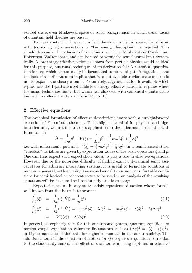
220 Martin Bojowald
excited state, even Minkowski space or other backgrounds on which usual vacuaof quantum field theories are based.
To make contact with quantum field theory on a curved spacetime, or evenwith (cosmological) observations, a “low energy description” is required. Thisshould determine the behavior of excitations near local Minkowski or Friedmann–Robertson–Walker space, and can be used to verify the semiclassical limit dynam-ically. A low energy effective action as known from particle physics would be idealfor this purpose, but usual techniques of its derivation fail: A canonical quantiza-tion is used which cannot easily be formulated in terms of path integrations, andthe lack of a useful vacuum implies that it is not even clear what state one coulduse to expand the theory around. Fortunately, a generalization is available whichreproduces the 1-particle irreducible low energy effective action in regimes wherethe usual techniques apply, but which can also deal with canonical quantizationsand with a different state structure [14, 15, 16].
2. Effective equations
The canonical formulation of effective descriptions starts with a straightforwardextension of Ehrenfest’s theorem. To highlight several of its physical and alge-braic features, we first illustrate its application to the anharmonic oscillator withHamiltonian
H =1
2mp2 + V (q) =
12m
p2 +12mω2q2 +
13λq3
i.e. with anharmonic potential V (q) = 12mω2q2 + 1
3λq3. In a semiclassical state,
“classical” variables are given by expectation values of the basic operators q and p.One can thus expect such expectation values to play a role in effective equations.However, due to the notorious difficulty of finding explicit dynamical semiclassi-cal states for arbitrary interacting systems, it is useful to formulate equations ofmotion in general, without using any semiclassicality assumptions. Suitable condi-tions for semiclassical or coherent states to be used in an analysis of the resultingequations will be discussed self-consistently at a later stage.
Expectation values in any state satisfy equations of motion whose form iswell-known from the Ehrenfest theorem:
ddt〈q〉 =
1i�〈[q, H ]〉 =
1m〈p〉 (2.1)
ddt〈p〉 =
1i�〈[p, H ]〉 = −mω2〈q〉 − λ〈q2〉 = −mω2〈q〉 − λ〈q〉2 − λ(Δq)2
= −V ′(〈q〉)− λ(Δq)2 . (2.2)
In general, as explicitly seen for this anharmonic system, quantum equations ofmotion couple expectation values to fluctuations such as (Δq)2 = 〈(q − 〈q〉)2〉,or higher moments of the state for higher monomials in the anharmonicity. Theadditional term in the equation of motion for 〈p〉 requires a quantum correctionto the classical dynamics. The effect of such terms is being captured in effective
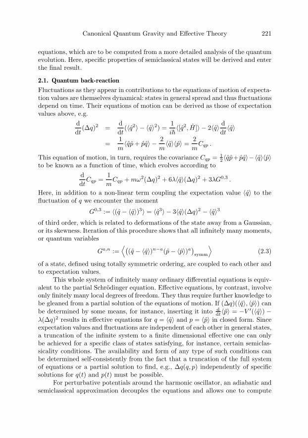
Canonical Quantum Gravity and Effective Theory 221
equations, which are to be computed from a more detailed analysis of the quantumevolution. Here, specific properties of semiclassical states will be derived and enterthe final result.
2.1. Quantum back-reaction
Fluctuations as they appear in contributions to the equations of motion of expecta-tion values are themselves dynamical: states in general spread and thus fluctuationsdepend on time. Their equations of motion can be derived as those of expectationvalues above, e.g.
ddt
(Δq)2 =ddt
(〈q2〉 − 〈q〉2) =1i�〈[q2, H ]〉 − 2〈q〉 d
dt〈q〉
=1m〈qp + pq〉 − 2
m〈q〉〈p〉 =
2mCqp .
This equation of motion, in turn, requires the covariance Cqp = 12 〈qp+ pq〉−〈q〉〈p〉
to be known as a function of time, which evolves according toddt
Cqp =1mCqp + mω2(Δq)2 + 6λ〈q〉(Δq)2 + 3λG0,3 .
Here, in addition to a non-linear term coupling the expectation value 〈q〉 to thefluctuation of q we encounter the moment
G0,3 := 〈(q − 〈q〉)3〉 = 〈q3〉 − 3〈q〉(Δq)2 − 〈q〉3
of third order, which is related to deformations of the state away from a Gaussian,or its skewness. Iteration of this procedure shows that all infinitely many moments,or quantum variables
Ga,n :=⟨(
(q − 〈q〉)n−a(p− 〈p〉)a)symm
⟩(2.3)
of a state, defined using totally symmetric ordering, are coupled to each other andto expectation values.
This whole system of infinitely many ordinary differential equations is equiv-alent to the partial Schrodinger equation. Effective equations, by contrast, involveonly finitely many local degrees of freedom. They thus require further knowledge tobe gleaned from a partial solution of the equations of motion. If (Δq)(〈q〉, 〈p〉) canbe determined by some means, for instance, inserting it into d
dt〈p〉 = −V ′(〈q〉) −λ(Δq)2 results in effective equations for q = 〈q〉 and p = 〈p〉 in closed form. Sinceexpectation values and fluctuations are independent of each other in general states,a truncation of the infinite system to a finite dimensional effective one can onlybe achieved for a specific class of states satisfying, for instance, certain semiclas-sicality conditions. The availability and form of any type of such conditions canbe determined self-consistently from the fact that a truncation of the full systemof equations or a partial solution to find, e.g., Δq(q, p) independently of specificsolutions for q(t) and p(t) must be possible.
For perturbative potentials around the harmonic oscillator, an adiabatic andsemiclassical approximation decouples the equations and allows one to compute
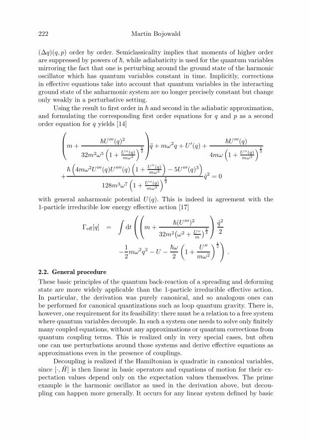
222 Martin Bojowald
(Δq)(q, p) order by order. Semiclassicality implies that moments of higher orderare suppressed by powers of �, while adiabaticity is used for the quantum variablesmirroring the fact that one is perturbing around the ground state of the harmonicoscillator which has quantum variables constant in time. Implicitly, correctionsin effective equations take into account that quantum variables in the interactingground state of the anharmonic system are no longer precisely constant but changeonly weakly in a perturbative setting.
Using the result to first order in � and second in the adiabatic approximation,and formulating the corresponding first order equations for q and p as a secondorder equation for q yields [14]⎛⎜⎝m +
�U ′′′(q)2
32m2ω5(1 + U ′′(q)
mω2
) 52
⎞⎟⎠q + mω2q + U ′(q) +�U ′′′(q)
4mω(1 + U ′′(q)
mω2
) 12
+�(4mω2U ′′′(q)U ′′′′(q)
(1 + U ′′(q)
mω2
)− 5U ′′′(q)3
)128m3ω7
(1 + U ′′(q)
mω2
) 72
q2 = 0
with general anharmonic potential U(q). This is indeed in agreement with the1-particle irreducible low energy effective action [17]
Γeff [q] =∫
dt
⎛⎝⎛⎝m +�(U ′′′)2
32m2(ω2 + U ′′
m
) 52
⎞⎠ q2
2
−12mω2q2 − U − �ω
2
(1 +
U ′′
mω2
) 12)
.
2.2. General procedure
These basic principles of the quantum back-reaction of a spreading and deformingstate are more widely applicable than the 1-particle irreducible effective action.In particular, the derivation was purely canonical, and so analogous ones canbe performed for canonical quantizations such as loop quantum gravity. There is,however, one requirement for its feasibility: there must be a relation to a free systemwhere quantum variables decouple. In such a system one needs to solve only finitelymany coupled equations, without any approximations or quantum corrections fromquantum coupling terms. This is realized only in very special cases, but oftenone can use perturbations around those systems and derive effective equations asapproximations even in the presence of couplings.
Decoupling is realized if the Hamiltonian is quadratic in canonical variables,since [·, H ] is then linear in basic operators and equations of motion for their ex-pectation values depend only on the expectation values themselves. The primeexample is the harmonic oscillator as used in the derivation above, but decou-pling can happen more generally. It occurs for any linear system defined by basic

Canonical Quantum Gravity and Effective Theory 223
variables Ji which (i) form a linear commutator algebra and (ii) have a linearcombination which equals the Hamiltonian H. This will be used later in quantumcosmology.
Given a linear system, one can explicitly solve its equations of motion forquantum variables, determining the moments of its dynamical coherent states.For perturbations around such a system one obtains coupled equations and has toanalyze their form to find suitable conditions and approximations in which theycan be truncated. While one often makes use of a semiclassical approximation tojustify ignoring most of the quantum variables, other steps such as the adiabaticityassumption used for the low energy effective action may not always be valid. Thisassumption is based on more specific properties of the solvable system, namelythe fact that the ground state of the harmonic oscillator has constant quantumvariables. They can thus remain adiabatic even under perturbations of the system.But not all linear systems have a ground (or other) state with constant quantumvariables and there may be no other way to realize adiabaticity. Then, the Ga,n maynot be solvable explicitly as functions of Ji which one could then insert into theequations of motion for expectation values. Still, the semiclassical approximationallows a decoupling of almost all quantum variables; one will, to a given order, onlyhave to keep a finite number of them as independent quantum degrees of freedomin addition to the classical-type expectation values. In this way, one obtains higherdimensional effective systems which are dynamical systems formulated in terms ofmore than just the classical variables. In addition to quantum correction termssuch as those in an effective potential, such systems have additional variables andequations for true quantum degrees of freedom.
This emphasis on observables, i.e. expectation values, fluctuations and othermoments, rather than states provides a more algebraic viewpoint which has ad-ditional advantages beyond the fact that one obtains a good approximation toquantum behavior. By directly solving equations of motion for moments, ratherthan first solving for a state and then integrating out to obtain moments, onecan bypass a calculational step which is often analytically difficult or numericallytime consuming. Especially in semiclassical regimes states are often highly oscilla-tory, which would require numerical integrations in expectation values with veryfine resolutions. This can be avoided by directly using numerical solutions to thecoupled equations for expectation values and some moments. Also analytically,after one successfully truncated the infinite set of equations by semiclassical orother approximations, one has only one step of solving coupled ordinary differen-tial equations instead of solving a partial differential equation for the state andthen still having to integrate it to find observables of real interest.
The procedure has an underlying geometrical picture [18, 19, 20]: The dynam-ics is formulated on the quantum phase space which is given by the (projective)Hilbert space. Points in the phase space are thus states, and so are tangent vec-tors since the Hilbert space is linear. The symplectic form as a 2-form is then anantisymmetric bilinear form which one can define as Ω(·, ·) = 2�Im〈·|·〉 in terms
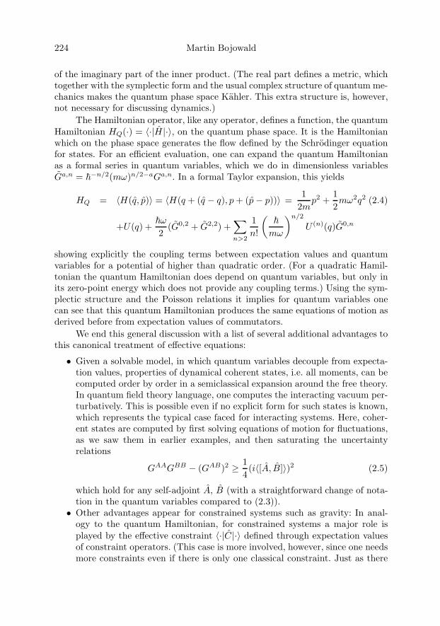
224 Martin Bojowald
of the imaginary part of the inner product. (The real part defines a metric, whichtogether with the symplectic form and the usual complex structure of quantum me-chanics makes the quantum phase space Kahler. This extra structure is, however,not necessary for discussing dynamics.)
The Hamiltonian operator, like any operator, defines a function, the quantumHamiltonian HQ(·) = 〈·|H |·〉, on the quantum phase space. It is the Hamiltonianwhich on the phase space generates the flow defined by the Schrodinger equationfor states. For an efficient evaluation, one can expand the quantum Hamiltonianas a formal series in quantum variables, which we do in dimensionless variablesGa,n = �−n/2(mω)n/2−aGa,n. In a formal Taylor expansion, this yields
HQ = 〈H(q, p)〉 = 〈H(q + (q − q), p + (p− p))〉 =1
2mp2 +
12mω2q2 (2.4)
+U(q) +�ω2
(G0,2 + G2,2) +∑n>2
1n!
(�
mω
)n/2
U (n)(q)G0,n
showing explicitly the coupling terms between expectation values and quantumvariables for a potential of higher than quadratic order. (For a quadratic Hamil-tonian the quantum Hamiltonian does depend on quantum variables, but only inits zero-point energy which does not provide any coupling terms.) Using the sym-plectic structure and the Poisson relations it implies for quantum variables onecan see that this quantum Hamiltonian produces the same equations of motion asderived before from expectation values of commutators.
We end this general discussion with a list of several additional advantages tothis canonical treatment of effective equations:
• Given a solvable model, in which quantum variables decouple from expecta-tion values, properties of dynamical coherent states, i.e. all moments, can becomputed order by order in a semiclassical expansion around the free theory.In quantum field theory language, one computes the interacting vacuum per-turbatively. This is possible even if no explicit form for such states is known,which represents the typical case faced for interacting systems. Here, coher-ent states are computed by first solving equations of motion for fluctuations,as we saw them in earlier examples, and then saturating the uncertaintyrelations
GAAGBB − (GAB)2 ≥ 14(i〈[A, B]〉)2 (2.5)
which hold for any self-adjoint A, B (with a straightforward change of nota-tion in the quantum variables compared to (2.3)).
• Other advantages appear for constrained systems such as gravity: In anal-ogy to the quantum Hamiltonian, for constrained systems a major role isplayed by the effective constraint 〈·|C|·〉 defined through expectation valuesof constraint operators. (This case is more involved, however, since one needsmore constraints even if there is only one classical constraint. Just as there
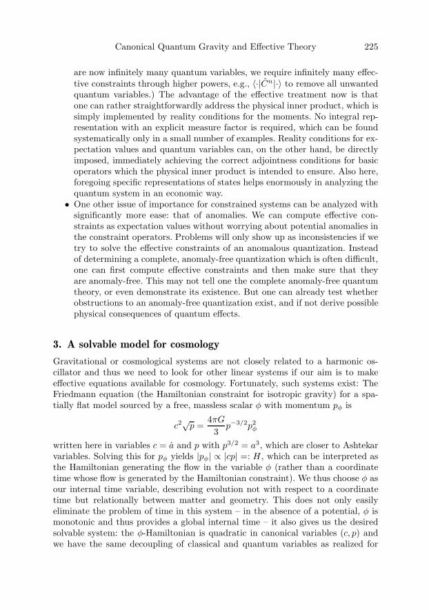
Canonical Quantum Gravity and Effective Theory 225
are now infinitely many quantum variables, we require infinitely many effec-tive constraints through higher powers, e.g., 〈·|Cn|·〉 to remove all unwantedquantum variables.) The advantage of the effective treatment now is thatone can rather straightforwardly address the physical inner product, which issimply implemented by reality conditions for the moments. No integral rep-resentation with an explicit measure factor is required, which can be foundsystematically only in a small number of examples. Reality conditions for ex-pectation values and quantum variables can, on the other hand, be directlyimposed, immediately achieving the correct adjointness conditions for basicoperators which the physical inner product is intended to ensure. Also here,foregoing specific representations of states helps enormously in analyzing thequantum system in an economic way.
• One other issue of importance for constrained systems can be analyzed withsignificantly more ease: that of anomalies. We can compute effective con-straints as expectation values without worrying about potential anomalies inthe constraint operators. Problems will only show up as inconsistencies if wetry to solve the effective constraints of an anomalous quantization. Insteadof determining a complete, anomaly-free quantization which is often difficult,one can first compute effective constraints and then make sure that theyare anomaly-free. This may not tell one the complete anomaly-free quantumtheory, or even demonstrate its existence. But one can already test whetherobstructions to an anomaly-free quantization exist, and if not derive possiblephysical consequences of quantum effects.
3. A solvable model for cosmology
Gravitational or cosmological systems are not closely related to a harmonic os-cillator and thus we need to look for other linear systems if our aim is to makeeffective equations available for cosmology. Fortunately, such systems exist: TheFriedmann equation (the Hamiltonian constraint for isotropic gravity) for a spa-tially flat model sourced by a free, massless scalar φ with momentum pφ is
c2√p =
4πG3
p−3/2p2φ
written here in variables c = a and p with p3/2 = a3, which are closer to Ashtekarvariables. Solving this for pφ yields |pφ| ∝ |cp| =: H , which can be interpreted asthe Hamiltonian generating the flow in the variable φ (rather than a coordinatetime whose flow is generated by the Hamiltonian constraint). We thus choose φ asour internal time variable, describing evolution not with respect to a coordinatetime but relationally between matter and geometry. This does not only easilyeliminate the problem of time in this system – in the absence of a potential, φ ismonotonic and thus provides a global internal time – it also gives us the desiredsolvable system: the φ-Hamiltonian is quadratic in canonical variables (c, p) andwe have the same decoupling of classical and quantum variables as realized for

226 Martin Bojowald
the harmonic oscillator. (In fact, a simple canonical transformation shows that theHamiltonian cp is an upside-down harmonic oscillator.)
The easy availability of a global internal time and the structure of the con-straint equation were exploited in [21, 22] to determine the physical Hilbert spaceof this system by techniques known from the Klein–Gordon particle, and to analyzesome solutions given by Gaussian initial states numerically. The solvable nature ofthis system was realized in [23], which explained several features of the numericalsolutions which were unexpected from general experience of quantum systems.
Quantum equations of motion for the solvable system with Hamiltonian1
H = cp are
c = c , p = p , G0,2 = 2G0,2 , G1,2 = 0 , G2,2 = −2G2,2
and so on for higher moments, which are easily solved by c(t) = c1et, p(t) = c2e
−t,G0,2(t) = c3e
−2t, G1,2(t) = c4 and G2,2(t) = c5e2t. The solution for p directly
shows the classical singularity since p = 0 is reached for φ → ∞ which, as onecan check by gauging the system, corresponds to a finite proper time interval. Oneclearly sees here that the classical singularity is realized in the same way when thesystem is quantized in the Schrodinger representation, as done in Wheeler–DeWittquantum cosmology. In fact, due to the solvability there are no quantum correctionterms whatsoever, and the quantum equations of motion for expectation values areexactly the same as the classical equations of motion.
For semiclassical issues, one can analyze the solutions for fluctuations. Theyare subject to the uncertainty relation
G0,2G2,2 − (G1,2)2 ≥ 14
�2 (3.1)
which for the constants of integration in our general solutions implies c3c5 ≥ �2/4+c24. If a state is initially chosen to be semiclassical, this property is preserved duringevolution: we have constant relative spreads (Δp)/p =
√G2,2/p and (Δc)/c =√
G0,2/c. This also illustrates why the classical singularity cannot be resolved:There are simply no significant quantum effects in this system, no matter howclose we get to the classical singularity.
This is different in a loop formulation. Here, in loop quantum cosmology[25, 26], we do not have an operator for a connection component like c, but onlyfor holonomies as basic operators. While the precise form of a loop quantizedHamiltonian constraint can be complicated, the main effect is that now a periodicfunction such as sin c replaces c in the Friedmann equation. This provides a typeof quantum geometry effect through the addition of higher powers of extrinsiccurvature. We now expect deviations from classical behavior when c becomes large,just when we approach the classical big bang singularity.
But it also means that the loop Hamiltonian H = p sin c now is non-quadraticin canonical variables and thus, in this form, not solvable. The corresponding
1Note that we are dropping the absolute value to have a truly quadratic Hamiltonian. This canbe shown to be a safe procedure when properties of semiclassical states are of interest [24].
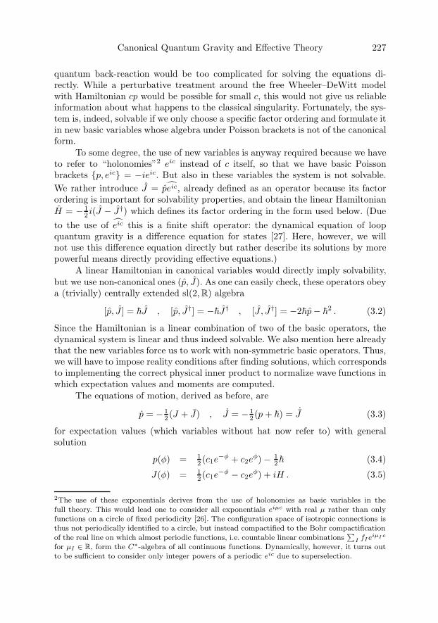
Canonical Quantum Gravity and Effective Theory 227
quantum back-reaction would be too complicated for solving the equations di-rectly. While a perturbative treatment around the free Wheeler–DeWitt modelwith Hamiltonian cp would be possible for small c, this would not give us reliableinformation about what happens to the classical singularity. Fortunately, the sys-tem is, indeed, solvable if we only choose a specific factor ordering and formulate itin new basic variables whose algebra under Poisson brackets is not of the canonicalform.
To some degree, the use of new variables is anyway required because we haveto refer to “holonomies”2 eic instead of c itself, so that we have basic Poissonbrackets {p, eic} = −ieic. But also in these variables the system is not solvable.We rather introduce J = peic, already defined as an operator because its factorordering is important for solvability properties, and obtain the linear HamiltonianH = − 1
2 i(J − J†) which defines its factor ordering in the form used below. (Dueto the use of eic this is a finite shift operator: the dynamical equation of loopquantum gravity is a difference equation for states [27]. Here, however, we willnot use this difference equation directly but rather describe its solutions by morepowerful means directly providing effective equations.)
A linear Hamiltonian in canonical variables would directly imply solvability,but we use non-canonical ones (p, J). As one can easily check, these operators obeya (trivially) centrally extended sl(2,R) algebra
[p, J ] = �J , [p, J†] = −�J† , [J , J†] = −2�p− �2 . (3.2)
Since the Hamiltonian is a linear combination of two of the basic operators, thedynamical system is linear and thus indeed solvable. We also mention here alreadythat the new variables force us to work with non-symmetric basic operators. Thus,we will have to impose reality conditions after finding solutions, which correspondsto implementing the correct physical inner product to normalize wave functions inwhich expectation values and moments are computed.
The equations of motion, derived as before, are
p = − 12 (J + J) , J = − 1
2 (p + �) = ˙J (3.3)
for expectation values (which variables without hat now refer to) with generalsolution
p(φ) = 12 (c1e−φ + c2e
φ)− 12� (3.4)
J(φ) = 12 (c1e−φ − c2e
φ) + iH . (3.5)
2The use of these exponentials derives from the use of holonomies as basic variables in thefull theory. This would lead one to consider all exponentials eiμc with real μ rather than onlyfunctions on a circle of fixed periodicity [26]. The configuration space of isotropic connections isthus not periodically identified to a circle, but instead compactified to the Bohr compactificationof the real line on which almost periodic functions, i.e. countable linear combinations
∑I fIeiμI c
for μI ∈ R, form the C∗-algebra of all continuous functions. Dynamically, however, it turns outto be sufficient to consider only integer powers of a periodic eic due to superselection.

228 Martin Bojowald
In contrast to the Wheeler–DeWitt model, we indeed see a resolution of the clas-sical singularity: There is a “bounce” in the sense that |p| → ∞ for φ → ±∞.However, without further analysis one could not be sure that the state does notenter the quantum regime too deeply, where other quantum geometry correctionsnot included in the solvable model would set in (e.g. those of [28], based on [43] inthe full theory).
The model itself could thus break down, invalidating the naive conclusionabout the bounce. In particular, the solutions show that, for c1c2 < 0, p canbecome zero where the model could no longer be trusted. (Nevertheless, the un-derlying difference equation is non-singular since it extends the wave functionuniquely through the classical singularity [29, 30]. But this behavior of the wavefunction itself does not easily provide an effective or geometrical picture of howthe classical singularity is resolved.) The precise form in which a deep quantumregime could be entered depends, by its very nature, on details of the quantummodel, in particular the factor ordering of the constraint. There may be choicesfor which the expectation value of p never becomes zero, but this does not rule outthat a deep quantum regime can be entered, where the model would break down.In any case one has to provide a detailed analysis if one tries to justify the bounceunder general conditions.
The situation is simpler when one assumes that a state starts out semiclassi-cally at large volume, and then follows its evolution to smaller scales and possiblyback to larger ones after a bounce. As in the Wheeler–DeWitt model, the statewould not change its semiclassicality properties strongly while it is still at ratherlarge volume. Semiclassicality properties can, however, change in the bounce tran-sition between two branches.
For a correct analysis of the corresponding solutions we now have to imposethe reality conditions. Classically we have JJ = p2 for J = p exp(ic). Whenquantized, exp(ic) must become an unitary operator on the physical Hilbert space,which implies reality conditions for our basic operators. Although we use J insteadof eic and cannot directly implement unitarity, there is a similar condition relatedto unitarity for the basic operators: J J† = p2. This is not linear, and so takingan expectation values of this relation provides a condition involving expectationvalues as well as fluctuations,
|J |2 − (p + 12�)2 = 1
4�2 −GJJ + Gpp . (3.6)
(We are now denoting the second order quantum variables by subscripts of theoperators used. This is more convenient than the notation Ga,n because we haveto distinguish between J and J† in addition to p.)
Inserting solutions, this implies c1c2 = H2 +O(�) for the expectation valueswhere we assumed an initial semiclassical state where fluctuations contribute onlyterms of the order �. Since this relation only depends on constants of motion(including the O(�)-terms since one can see easily that GJJ−Gpp is preserved), it is
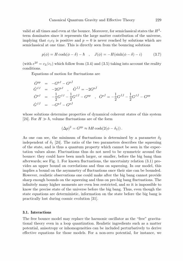
Canonical Quantum Gravity and Effective Theory 229
valid at all times and even at the bounce. Moreover, for semiclassical states the H2-term dominates since it represents the large matter contribution of the universe,implying that c1c2 is positive and p = 0 is never reached by solutions which aresemiclassical at one time. This is directly seen from the bouncing solutions
p(φ) = H cosh(φ− δ)− � , J(φ) = −H(sinh(φ− δ)− i) (3.7)
(with e2δ = c2/c1) which follow from (3.4) and (3.5) taking into account the realityconditions.
Equations of motion for fluctuations are
Gpp = −GpJ −GpJ
GJJ = −2GpJ , GJJ = −2GpJ
GpJ = −12GJJ − 1
2GJJ −Gpp , GpJ = −1
2GJJ − 1
2GJJ −Gpp
GJJ = −GpJ −GpJ
whose solutions determine properties of dynamical coherent states of this system[24]. For H * �, volume fluctuations are of the form
(Δp)2 = Gpp ≈ �H cosh(2(φ− δ2)) .
As one can see, the minimum of fluctuations is determined by a parameter δ2independent of δ1 [24]. The ratio of the two parameters describes the squeezingof the state, and is thus a quantum property which cannot be seen in the expec-tation values alone. Fluctuations thus do not need to be symmetric around thebounce: they could have been much larger, or smaller, before the big bang thanafterwards; see Fig. 1. For known fluctuations, the uncertainty relation (3.1) pro-vides an upper bound on correlations and thus on squeezing. In our model, thisimplies a bound on the asymmetry of fluctuations once their size can be bounded.However, realistic observations one could make after the big bang cannot providesharp enough bounds on the squeezing and thus on pre-big bang fluctuations. Theinfinitely many higher moments are even less restricted, and so it is impossible toknow the precise state of the universe before the big bang. Thus, even though thestate equations are deterministic, information on the state before the big bang ispractically lost during cosmic evolution [31].
3.1. Interactions
The free bounce model may replace the harmonic oscillator as the “free” gravita-tional theory even in a loop quantization. Realistic ingredients such as a matterpotential, anisotropy or inhomogeneities can be included perturbatively to deriveeffective equations for those models. For a non-zero potential, for instance, we
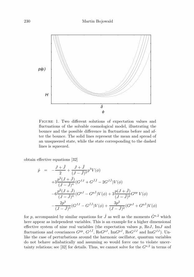
230 Martin Bojowald
H
δ
p( ) φ
φ
Figure 1. Two different solutions of expectation values andfluctuations of the solvable cosmological model, illustrating thebounce and the possible difference in fluctuations before and af-ter the bounce. The solid lines represent the mean and spread ofan unsqueezed state, while the state corresponding to the dashedlines is squeezed.
obtain effective equations [32]
p = −J + J
2+
J + J
(J − J)2p3V (φ)
+3p3(J + J)(J − J)4
(GJJ + GJ J − 2GJJ)V (φ)
−6p2(J + J)(J − J)3
(GpJ −GpJ )V (φ) + 3p(J + J)(J − J)2
Gpp V (φ)
− 2p3
(J − J)3(GJJ −GJ J)V (φ) +
3p2
(J − J)2(GpJ + GpJ )V (φ)
for p, accompanied by similar equations for J as well as the moments Ga,2 whichhere appear as independent variables. This is an example for a higher dimensionaleffective system of nine real variables (the expectation values p, ReJ , ImJ andfluctuations and covariances Gpp, GJJ , ReGpJ , ImGpJ , ReGJJ and ImGJJ ). Un-like the case of perturbations around the harmonic oscillator, quantum variablesdo not behave adiabatically and assuming so would force one to violate uncer-tainty relations; see [32] for details. Thus, we cannot solve for the Ga,2 in terms of

Canonical Quantum Gravity and Effective Theory 231
expectation values directly, and rather have to keep them as independent variablesin a higher dimensional effective system.
4. Effective quantum gravity
Many field theoretical issues present in this approach to effective equations remainto be worked out, which would be required for an application to quantum gravitybeyond cosmological models. In this context, it is encouraging that variables sim-ilar to the Ga,n were used in early (non-canonical) developments of effective fieldtheories in the context of symmetry breaking [33, 34]. Some difficulties may beovercome by using a mode decomposition of fields, made possible by the choice ofa background geometry which enters the effective description as part of the semi-classical states used. This strategy is applied to inflationary structure formationin [35].
For loop quantum gravity, moreover, one may be in a manageable situationbecause the discreteness of graphs implies essentially a finite number of degreesof freedom in any finite volume, in contrast to infinitely many ones in ordinaryquantum field theory. One can thus use moments between all independent graph-associated degrees of freedom, and then perform a continuum approximation forthe resulting effective expressions. Only after performing this limit would the infin-itely many degrees of freedom of the classical theory arise. This procedure, withoutexplicitly computing all quantum correction terms, is outlined in [36].
This allows one to apply existing techniques available for the derivation ofeffective systems to a derivation of cosmological perturbation equations [37, 38, 39,40, 41]. As a result one obtains quantum corrections arising from the loop quanti-zation, which can then be directly analyzed in cosmological phenomenology, or forfundamental questions such as the issue of local Lorentz invariance at low energies.Moreover, from a combination of the perturbation equations one can recover theNewton potential to classical order and also here derive quantum corrections.
As already mentioned, one can also study some part of the anomaly issue ofconstrained systems at the effective level. Effective constraints can first be com-puted from operators which have not yet been checked for possible anomalies. Forthe effective constraints anomalies can then be analyzed much more straightfor-wardly by computing their Poisson algebra. Even before complete effective con-straints have been computed, which is so far not available in inhomogeneous sys-tems, one may include only one type of quantum corrections into an incompleteeffective constraint. In addition to quantum back-reaction effects, whose computa-tion is typically most involved, there are several effects arising from the discrete-ness of quantum geometry. The latter include higher order terms due to the use ofholonomies in the basic representation, and corrections to inverse densitized triadcomponents [42, 43]. Any of these terms can be introduced as part of an effectiveconstraint, and their effect on anomalies studied in separation.

232 Martin Bojowald
There have recently been several results in particular for inverse triad cor-rections: Such non-trivial quantum corrections are possible even for anomaly-freeconstraints. This is rather surprising as it has often been expected that quantumcorrections due to the underlying discreteness necessarily break covariance. As thecalculations show, this may happen for some form of the corrections, and pos-sible quantization ambiguities which may exist at the kinematical level are thusrestricted. But anomaly-freedom does not require such quantum corrections tobe completely absent and allows non-trivial quantum effects in a covariant quan-tum space-time. Specific cases which have been dealt with in this way includethe linearized cosmological mode equations of [39, 40, 44] and the fully non-linearspherically symmetric vacuum sector [45].
A different issue is the performance of the continuum limit for a sector ofthe quantum theory defined by introducing a background via a specific class ofstates (such as those of semiclassical geometries peaked at the given background).Although one would not usually need to perform such a limit, given that thefull theory is already a continuum quantum theory, it is of interest for makingcontact with local quantum field theory on a background. At this point, one expectsthat renormalization would have to be performed, whose role in discrete quantumgravity could thus be studied.
Acknowledgement
Work described here was supported in part by NSF grants PHY-0554771 andPHY-0653127.
References
[1] C. Rovelli, Quantum Gravity, Cambridge University Press, Cambridge, UK, 2004.
[2] A. Ashtekar and J. Lewandowski, Background independent quantum gravity: A statusreport Class. Quantum Grav. 21 (2004), R53–R152, [gr-qc/0404018].
[3] T. Thiemann, Introduction to Modern Canonical Quantum General Relativity, [gr-qc/0110034].
[4] A. Ashtekar, New Hamiltonian Formulation of General Relativity Phys. Rev. D 36(1987), 1587–1602.
[5] J. F. Barbero G., Real Ashtekar Variables for Lorentzian Signature Space-TimesPhys. Rev. D 51 (1995), 5507–5510, [gr-qc/9410014].
[6] J. Lewandowski, A. Oko�low, H. Sahlmann, and T. Thiemann, Uniqueness of dif-feomorphism invariant states on holonomy-flux algebras Commun. Math. Phys. 267(2006), 703–733, [gr-qc/0504147].
[7] C. Fleischhack, Representations of the Weyl Algebra in Quantum Geometry, [math-ph/0407006].
[8] M. Varadarajan, Towards new background independent representations for LoopQuantum Gravity, [arXiv:0709.1680].
[9] G. Immirzi, Real and Complex Connections for Canonical Gravity Class. QuantumGrav. 14 (1997), L177–L181.
Canonical Quantum Gravity and Effective Theory 233
[10] A. Ashtekar, J. Lewandowski, D. Marolf, J. Mourao, and T. Thiemann, Quantizationof Diffeomorphism Invariant Theories of Connections with Local Degrees of FreedomJ. Math. Phys. 36 (1995), 6456–6493, [gr-qc/9504018].
[11] C. Rovelli and L. Smolin, Discreteness of Area and Volume in Quantum GravityNucl. Phys. B 442 (1995), 593–619, [gr-qc/9411005], Erratum: Nucl. Phys. B 456(1995) 753.
[12] A. Ashtekar and J. Lewandowski, Quantum Theory of Geometry I: Area OperatorsClass. Quantum Grav. 14 (1997), A55–A82, [gr-qc/9602046].
[13] A. Ashtekar and J. Lewandowski, Quantum Theory of Geometry II: Volume Opera-tors Adv. Theor. Math. Phys. 1 (1997), 388–429, [gr-qc/9711031].
[14] M. Bojowald and A. Skirzewski, Effective Equations of Motion for Quantum SystemsRev. Math. Phys. 18 (2006), 713–745, [math-ph/0511043].
[15] A. Skirzewski, Effective Equations of Motion for Quantum Systems, PhD thesis,Humboldt-Universitat Berlin, 2006.
[16] M. Bojowald and A. Skirzewski, Quantum Gravity and Higher Curvature ActionsInt. J. Geom. Math. Mod. Phys. 4 (2007), 25–52, [hep-th/0606232].
[17] F. Cametti, G. Jona-Lasinio, C. Presilla, and F. Toninelli, Comparison between quan-tum and classical dynamics in the effective action formalism Proceedings of the In-ternational School of Physics “Enrico Fermi”, Course CXLIII, pages 431–448 (IOSPress, Amsterdam, 2000), [quant-ph/9910065].
[18] T. W. B. Kibble, Geometrization of quantum mechanics Commun. Math. Phys. 65(1979), 189–201.
[19] A. Heslot, Quantum mechanics as a classical theory Phys. Rev. D 31 (1985), 1341–1348.
[20] A. Ashtekar and T. A. Schilling, Geometrical Formulation of Quantum Mechanics,In A. Harvey, editor, On Einstein’s Path: Essays in Honor of Engelbert Schucking,pages 23–65, Springer-Verlag, 1999, [gr-qc/9706069].
[21] A. Ashtekar, T. Pawlowski, and P. Singh, Quantum Nature of the Big Bang Phys.Rev. Lett. 96 (2006), 141301, [gr-qc/0602086].
[22] A. Ashtekar, T. Pawlowski, and P. Singh, Quantum Nature of the Big Bang: An Ana-lytical and Numerical Investigation Phys. Rev. D 73 (2006), 124038, [gr-qc/0604013].
[23] M. Bojowald, Large scale effective theory for cosmological bounces Phys. Rev. D 75(2007), 081301(R), [gr-qc/0608100].
[24] M. Bojowald, Dynamical coherent states and physical solutions of quantum cosmo-logical bounces Phys. Rev. D 75 (2007), 123512, [gr-qc/0703144].
[25] M. Bojowald, Isotropic Loop Quantum Cosmology Class. Quantum Grav. 19 (2002),2717–2741, [gr-qc/0202077].
[26] A. Ashtekar, M. Bojowald, and J. Lewandowski, Mathematical structure of loop quan-tum cosmology Adv. Theor. Math. Phys. 7 (2003), 233–268, [gr-qc/0304074].
[27] M. Bojowald, Loop Quantum Cosmology IV: Discrete Time Evolution Class. Quan-tum Grav. 18 (2001), 1071–1088, [gr-qc/0008053].
[28] M. Bojowald, Inverse Scale Factor in Isotropic Quantum Geometry Phys. Rev. D 64(2001), 084018, [gr-qc/0105067].
234 Martin Bojowald
[29] M. Bojowald, Absence of a Singularity in Loop Quantum Cosmology Phys. Rev. Lett.86 (2001), 5227–5230, [gr-qc/0102069].
[30] M. Bojowald, Singularities and Quantum Gravity AIP Conf. Proc. 910 (2007), 294–333, [gr-qc/0702144].
[31] M. Bojowald, What happened before the big bang? Nature Physics 3 (2007), 523–525.
[32] M. Bojowald, H. Hernandez, and A. Skirzewski, Effective equations forisotropic quantum cosmology including matter Phys. Rev. D 76 (2007), 063511,[arXiv:0706.1057].
[33] K. Symanzik, Renormalizable models with simple symmetry breaking I. Symmetrybreaking by a source term Comm. Math. Phys. 16 (1970), 48–80.
[34] L. Dolan and R. Jackiw, Gauge-invariant signal for gauge-symmetry breaking Phys.Rev. D 9 (1974), 2904–2912.
[35] M. Bojowald and A. Skirzewski, Effective theory for the cosmological generation ofstructure Adv. Sci. Lett., to appear.
[36] M. Bojowald, H. Hernandez, M. Kagan, and A. Skirzewski, Effective constraints ofloop quantum gravity Phys. Rev. D 75 (2007), 064022, [gr-qc/0611112].
[37] M. Bojowald, H. Hernandez, M. Kagan, P. Singh, and A. Skirzewski, Formationand evolution of structure in loop cosmology Phys. Rev. Lett. 98 (2007), 031301,[astro-ph/0611685].
[38] M. Bojowald, H. Hernandez, M. Kagan, P. Singh, and A. Skirzewski, Hamiltoniancosmological perturbation theory with loop quantum gravity corrections Phys. Rev. D74 (2006), 123512, [gr-qc/0609057].
[39] M. Bojowald and G. Hossain, Cosmological vector modes and quantum gravity effectsClass. Quantum Grav. 24 (2007), 4801–4816, [arXiv:0709.0872].
[40] M. Bojowald and G. Hossain, Quantum gravity corrections to gravitational wavedispersion Phys. Rev. D 77 (2008), 023508, [arXiv:0709.2365].
[41] M. Bojowald, G. Hossain, M. Kagan, D. Mulryne, N. Nunes, and S. Shankara-narayanan, in preparation.
[42] T. Thiemann, Quantum Spin Dynamics (QSD) Class. Quantum Grav. 15 (1998),839–873, [gr-qc/9606089].
[43] T. Thiemann, QSD V: Quantum Gravity as the Natural Regulator of Matter Quan-tum Field Theories Class. Quantum Grav. 15 (1998), 1281–1314, [gr-qc/9705019].
[44] M. Bojowald and F. Hinterleitner, Isotropic loop quantum cosmology with matterPhys. Rev. D 66 (2002), 104003, [gr-qc/0207038].
[45] M. Bojowald and J. D. Reyes, in preparation.
Martin BojowaldInstitute for Gravitation and the CosmosThe Pennsylvania State University104 Davey Lab, University Park, PA 16802, USAe-mail: [email protected]
Quantum Field TheoryB. Fauser, J. Tolksdorf and E. Zeidler, Eds., 235–259c© 2009 Birkhauser Verlag Basel/Switzerland
From Discrete Space-Time to Minkowski Space:Basic Mechanisms, Methods and Perspectives
Felix Finster
Abstract. This survey article reviews recent results on fermion systems indiscrete space-time and corresponding systems in Minkowski space. After abasic introduction to the discrete setting, we explain a mechanism of sponta-neous symmetry breaking which leads to the emergence of a discrete causalstructure. As methods to study the transition between discrete space-timeand Minkowski space, we describe a lattice model for a static and isotropicspace-time, outline the analysis of regularization tails of vacuum Dirac seaconfigurations, and introduce a Lorentz invariant action for the masses of theDirac seas. We mention the method of the continuum limit, which allows toanalyze interacting systems. Open problems are discussed.
Mathematics Subject Classification (2000). Primary 83C99; Secondary 70G75.
Keywords. discrete space-time, emergent space-time, special relativity, causal-ity, fermionic projector, Dirac sea.
1. Introduction
It is generally believed that the concept of a space-time continuum (like Minkowskispace or a Lorentzian manifold) should be modified for distances as small as thePlanck length. The principle of the fermionic projector [4] proposes a new modelof space-time, which should be valid down to the Planck scale. This model is in-troduced as a system of quantum mechanical wave functions defined on a finitenumber of space-time points and is referred to as a fermion system in discretespace-time. The interaction is described via a variational principle where we min-imize an action defined for the ensemble of wave functions. A-priori, there are norelations between the space-time points; in particular, there is no nearest-neighborrelation and no notion of causality. The idea is that these additional structures
I would like to thank the organizers of the workshop “Recent Developments in Quantum FieldTheory” (Leipzig, July 2007) for helpful discussions and encouragement. I thank Joel Smoller
and the referee for helpful comments on the manuscript.

236 Felix Finster
should be generated spontaneously. More precisely, in order to minimize the ac-tion, the wave functions form specific configurations; this can be visualized as a“self-organization” of the particles. As a consequence of this self-organization, thewave functions induce non-trivial relations between the space-time points. We thusobtain additional structures in space-time, and it is conjectured that, in a suitablelimit where the number of particles and space-time points tends to infinity, thesestructures should give rise to the local and causal structure of Minkowski space.In this limit, the configuration of the wave functions should go over to a Dirac seastructure.
This conjecture has not yet been proved, but recent results give a detailedpicture of the connection between discrete space-time and Minkowski space. Also,mathematical methods were developed to shed light on particular aspects of theproblem. In this survey article we report on the present status, explain basicmechanisms and outline the analytical methods used so far. The presentation isself-contained and non-technical. The paper concludes with a discussion of openproblems.
2. Fermion systems in discrete space-time
We begin with the basic definitions in the discrete setting (for more details see [5]).Let (H,<.|.>) be a finite-dimensional complex inner product space. Thus <.|.> islinear in its second and anti-linear in its first argument, and it is symmetric,
<Ψ | Φ> = <Φ |Ψ> for all Ψ,Φ ∈ H ,
and non-degenerate,
<Ψ | Φ> = 0 for all Φ ∈ H =⇒ Ψ = 0 .
In contrast to a scalar product, <.|.> need not be positive.A projector A in H is defined just as in Hilbert spaces as a linear operator
which is idempotent and self-adjoint,
A2 = A and <AΨ |Φ> = <Ψ | AΦ> for all Ψ,Φ ∈ H .
Let M be a finite set. To every point x ∈ M we associate a projector Ex. Weassume that these projectors are orthogonal and complete in the sense that
Ex Ey = δxy Ex and∑x∈M
Ex = 11 . (1)
Furthermore, we assume that the images Ex(H) ⊂ H of these projectors are non-degenerate subspaces of H , which all have the same signature (n, n). We referto n as the spin dimension. The points x ∈ M are called discrete space-timepoints, and the corresponding projectors Ex are the space-time projectors. Thestructure (H,<.|.>, (Ex)x∈M ) is called discrete space-time.
We next introduce the so-called fermionic projector P as a projector in Hwhose image P (H) ⊂ H is negative definite. The vectors in the image of P havethe interpretation as the quantum states of the particles of our system. Thus the
From Discrete Space-Time to Minkowski Space 237
rank of P gives the number of particles f := dimP (H). The name “fermionicprojector” is motivated from the correspondence to Minkowski space, where ourparticles should go over to Dirac particles, being fermions (see Section 6 below).We call the obtained structure (H,<.|.>, (Ex)x∈M , P ) a fermion system in discretespace-time. Note that our definitions involve only three integer parameters: the spindimension n, the number of space-time points m, and the number of particles f .
The above definitions can be understood as a mathematical reduction tosome of the structures present in relativistic quantum mechanics, in such a waythat the Pauli Exclusion Principle, a local gauge principle and the equivalenceprinciple are respected (for details see [4, Chapter 3]). More precisely, describingthe many-particle system by a projector P , every vector Ψ ∈ H either lies in theimage of P or it does not. In this way, the fermionic projector encodes for everystate the occupation numbers 1 and 0, respectively, but it is impossible to describehigher occupation numbers. More technically, choosing a basis Ψ1, . . .Ψf of P (H),we can form the anti-symmetric many-particle wave function
Ψ = Ψ1 ∧ · · · ∧Ψf .
Due to the anti-symmetrization, this definition of Ψ is (up to a phase) indepen-dent of the choice of the basis Ψ1, . . . ,Ψf . In this way, we can associate to ev-ery fermionic projector a fermionic many-particle wave function, which clearlyrespects the Pauli exclusion principle. To reveal the local gauge principle, we con-sider unitary operators U (i.e. operators which for all Ψ,Φ ∈ H satisfy the relation<UΨ|UΦ> = <Ψ|Φ>) which do not change the space-time projectors,
Ex = UExU−1 for all x ∈M . (2)
We transform the fermionic projector according to
P → UPU−1 . (3)
Such transformations lead to physically equivalent fermion systems. The condi-tions (2) mean that U maps every subspace Ex(H) onto itself. In other words,U acts “locally” on the subspaces associated to the individual space-time points.The transformations (2, 3) can be identified with local gauge transformations inphysics (for details see [4, §3.1]). The equivalence principle is built into our frame-work in a very general form by the fact that our definitions do not distinguish anordering between the space-time points. Thus our definitions are symmetric underpermutations of the space-time points, generalizing the diffeomorphism invariancein general relativity.
Obviously, important physical principles are missing in our framework. Inparticular, our definitions involve no locality and no causality, and not even rela-tions like the nearest-neighbor relations on a lattice. The idea is that these ad-ditional structures, which are of course essential for the formulation of physics,should emerge as a consequence of a spontaneous symmetry breaking and a self-organization of the particles as described by a variational principle. Before explain-ing in more detail how this is supposed to work (Section 6), we first introduce the

238 Felix Finster
variational principle (Section 3), explain the mechanism of spontaneous symme-try breaking (Section 4), and discuss the emergence of a discrete causal structure(Section 5).
3. A variational principle
In order to introduce an interaction of the particles, we now set up a variationalprinciple. For any u ∈ H , we refer to the projection Exu ∈ Ex(H) as the localiza-tion of u at x. We also use the short notation u(x) = Exu and sometimes call u(x)the wave function corresponding to the vector u. Furthermore, we introduce theshort notation
P (x, y) = Ex P Ey , x, y ∈M . (4)This operator product maps Ey(H) ⊂ H to Ex(H), and it is often useful to regardit as a mapping only between these subspaces,
P (x, y) : Ey(H) → Ex(H) .
Using the properties of the space-time projectors (1), we find
(Pu)(x) = Ex Pu =∑y∈M
Ex P Ey u =∑y∈M
(Ex P Ey) (Ey u) ,
and thus(Pu)(x) =
∑y∈M
P (x, y) u(y) . (5)
This relation resembles the representation of an operator with an integral kernel,and thus we refer to P (x, y) as the discrete kernel of the fermionic projector. Nextwe introduce the closed chain Axy as the product
Axy := P (x, y) P (y, x) = Ex P Ey P Ex ; (6)
it maps Ex(H) to itself. Let λ1, . . . , λ2n be the roots of the characteristic poly-nomial of Axy, counted with multiplicities. We define the spectral weight |Axy|by
|Axy| =2n∑
j=1
|λj | .
Similarly, one can take the spectral weight of powers of Axy, and by summing overthe space-time points we get positive numbers depending only on the form of thefermionic projector relative to the space-time projectors. Our variational principleis to
minimize∑
x,y∈M
|A2xy| (7)
by considering variations of the fermionic projector which satisfy for a given realparameter κ the constraint ∑
x,y∈M
|Axy|2 = κ . (8)
From Discrete Space-Time to Minkowski Space 239
In the variation we also keep the number of particles f as well as discrete space-time fixed. Clearly, we need to choose κ such that there is at least one fermionicprojector which satisfies (8). It is easy to verify that (7) and (8) are invariant underthe transformations (2, 3), and thus our variational principle is gauge invariant.
The above variational principle was first introduced in [4]. In [5] it is analyzedmathematically, and it is shown in particular that minimizers exist:
Theorem 3.1. The minimum of the variational principle (7, 8) is attained.
Using the method of Lagrange multipliers, for every minimizer P there is areal parameter μ such that P is a stationary point of the action
Sμ[P ] =∑
x,y∈M
Lμ[Axy] (9)
with the LagrangianLμ[A] = |A2| − μ |A|2 . (10)
A useful method for constructing stationary points for a given value of the La-grange multiplier μ is to minimize the action Sμ without the constraint (8). Thisso-called auxiliary variational principle behaves differently depending on the valueof μ. If μ < 1
2n , the action is bounded from below, and it is proved in [5] that mini-mizers exist. In the case μ > 1
2n , on the other hand, the action is not bounded frombelow, and thus there are clearly no minimizers. In the remaining so-called criticalcase μ = 1
2n , partial existence results are given in [5], but the general existenceproblem is still open. The critical case is important for the physical applications.For simplicity, we omit the subscript μ = 1
2n and also refer to the auxiliary vari-ational principle in the critical case as the critical variational principle. Writingthe critical Lagrangian as
L[A] =14n
2n∑i,j=1
(|λi| − |λj |)2 , (11)
we get a good intuitive understanding of the critical variational principle: it triesto achieve that for every x, y ∈ M , all the roots of the characteristic polynomialof the closed chain Axy have the same absolute value.
We next derive the corresponding Euler-Lagrange equations (for details see [4,§3.5 and §5.2]). Suppose that P is a critical point of the action (9). We considera variation P (τ) of projectors with P (0) = P . Denoting the gradient of the La-grangian by M,
Mμ[A]αβ :=∂Lμ[A]
∂Aβα
, with α, β ∈ {1, . . . , 2n} , (12)
we can write the variation of the Lagrangian as a trace on Ex(H),
δLμ[Axy] =d
dτLμ[Axy(τ)]
∣∣∣τ=0
= Tr (ExMμ[Axy] δAxy) .

240 Felix Finster
Using the Leibniz rule
δAxy = δP (x, y) P (y, x) + P (x, y) δP (y, x)
together with the fact that the trace is cyclic, after summing over the space-timepoints we find ∑
x,y∈M
δLμ[Axy] =∑
x,y∈M
4 Tr (Ex Qμ(x, y) δP (y, x)) ,
where we set
Qμ(x, y) =14
(Mμ[Axy] P (x, y) + P (x, y)Mμ[Ayx]) . (13)
Thus the first variation of the action can be written as
δSμ[P ] = 4 Tr (Qμ δP ) , (14)
where Qμ is the operator in H with kernel (13). This equation can be simplifiedusing that the operators P (τ) are all projectors of fixed rank. Namely, there is afamily of unitary operators U(τ) with U(τ) = 11 and
P (τ) = U(τ)P U(τ)−1 .
Hence δP = i[B,P ], where we set B = −iU ′(0). Using this relation in (14) andagain using that the trace is cyclic, we find δSμ[P ] = 4iTr ([P,Qμ] B). Since B isan arbitrary self-adjoint operator, we conclude that
[P,Qμ] = 0 . (15)
This commutator equation with Qμ given by (13) are the Euler-Lagrange equationscorresponding to our variational principle.
4. A mechanism of spontaneous symmetry breaking
In the definition of fermion systems in discrete space-time, we did not distinguishan ordering of the space-time points; all our definitions are symmetric under per-mutations of the points of M . However, this does not necessarily mean that a givenfermion system will have this permutation symmetry. The simplest counterexam-ple is to take a fermionic projector consisting of one particle which is localized atthe first space-time point, i.e. in bra/ket-notation
P = −|u><u| with <u |u> = −1 andE1u = u , Exu = 0 for all x = 2, . . . ,m .
Then the fermionic projector distinguishes the first space-time point and thusbreaks the permutation symmetry. In [6] it is shown under general assumptions onthe number of particles and space-time points that, no matter how we choose thefermionic wave functions, it is impossible to arrange that the fermionic projectorrespects the permutation symmetry. In other words, the fermionic projector neces-sarily breaks the permutation symmetry of discrete space-time. We first specify the
From Discrete Space-Time to Minkowski Space 241
result and explain it afterwards. The group of all permutations of the space-timepoints is the symmetric group, denoted by Sm.
Definition 4.1. A subgroup O ⊂ Sm is called outer symmetry group of the fermionsystem in discrete space-time if for every σ ∈ O there is a unitary transformation Usuch that
UPU−1 = P and UExU−1 = Eσ(x) for all x ∈M . (16)
Theorem 4.2. (spontaneous breaking of the permutation symmetry) Suppose that(H,<.|.>, (Ex)x∈M , P ) is a fermion system in discrete space-time of spin dimen-sion n. Assume that the number of space-time points m is sufficiently large,
m >
{3 if n = 1
max(2n + 1, 4 [log2 n] + 6
)if n > 1
(17)
(where [x] is the Gauß bracket), and that the number of particles f lies in the range
n < f < m− 1 . (18)
Then the fermion system cannot have the outer symmetry group O = Sm.
For clarity we note that this theorem does not refer to the variational principleof Section 3. To explain the result, we now give an alternative proof in the simplestsituation where the theorem applies: the case n = 1, f = 2 and m = 4. For systemsof two particles, the following construction from [2] is very useful for visualizing thefermion system. The image of P is a two-dimensional, negative definite subspaceof H . Choosing an orthonormal basis (u1, u2) (i.e. <ui|uj> = −δij), the fermionicprojector can be written in bra/ket-notation as
P = −|u1><u1| − |u2><u2| . (19)
For any space-time point x ∈M we introduce the so-called local correlation matrixFx by
(Fx)ij = −<ui |Exuj> . (20)
The matrix Fx is Hermitian on the standard Euclidean C2. Thus we can decomposeit in the form
Fx =12
(ρx11 + �vx�σ) , (21)
where �σ = (σ1, σ2, σ3) are the Pauli matrices. We refer to the �vx as the Pauli vec-tors. The local correlation matrices are obviously invariant under unitary transfor-mations in H . But they do depend on the arbitrariness in choosing the orthonor-mal basis (u1, u2) of P (H). More precisely, the choice of the orthonormal basisinvolves a U(2)-freedom and, according to the transformation of Pauli spinors innon-relativistic quantum mechanics, this gives rise to orientation preserving rota-tions of all Pauli vectors. Hence the local correlation matrices are unique up to thetransformations
�vx −→ R�vx with R ∈ SO(3) . (22)
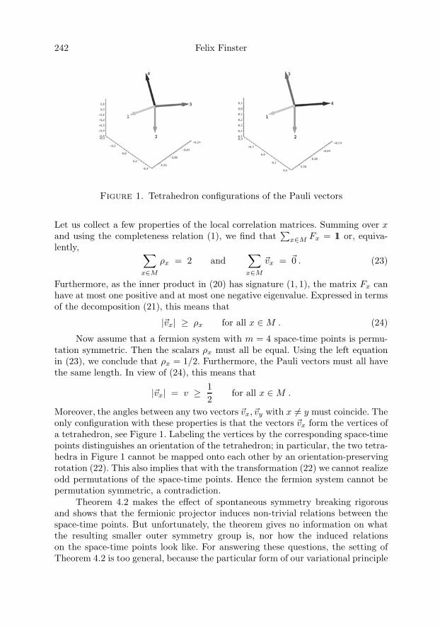
242 Felix Finster
Figure 1. Tetrahedron configurations of the Pauli vectors
Let us collect a few properties of the local correlation matrices. Summing over xand using the completeness relation (1), we find that
∑x∈M Fx = 11 or, equiva-
lently, ∑x∈M
ρx = 2 and∑x∈M
�vx = �0 . (23)
Furthermore, as the inner product in (20) has signature (1, 1), the matrix Fx canhave at most one positive and at most one negative eigenvalue. Expressed in termsof the decomposition (21), this means that
|�vx| ≥ ρx for all x ∈M . (24)
Now assume that a fermion system with m = 4 space-time points is permu-tation symmetric. Then the scalars ρx must all be equal. Using the left equationin (23), we conclude that ρx = 1/2. Furthermore, the Pauli vectors must all havethe same length. In view of (24), this means that
|�vx| = v ≥ 12
for all x ∈M .
Moreover, the angles between any two vectors �vx, �vy with x �= y must coincide. Theonly configuration with these properties is that the vectors �vx form the vertices ofa tetrahedron, see Figure 1. Labeling the vertices by the corresponding space-timepoints distinguishes an orientation of the tetrahedron; in particular, the two tetra-hedra in Figure 1 cannot be mapped onto each other by an orientation-preservingrotation (22). This also implies that with the transformation (22) we cannot realizeodd permutations of the space-time points. Hence the fermion system cannot bepermutation symmetric, a contradiction.
Theorem 4.2 makes the effect of spontaneous symmetry breaking rigorousand shows that the fermionic projector induces non-trivial relations between thespace-time points. But unfortunately, the theorem gives no information on whatthe resulting smaller outer symmetry group is, nor how the induced relationson the space-time points look like. For answering these questions, the setting ofTheorem 4.2 is too general, because the particular form of our variational principle
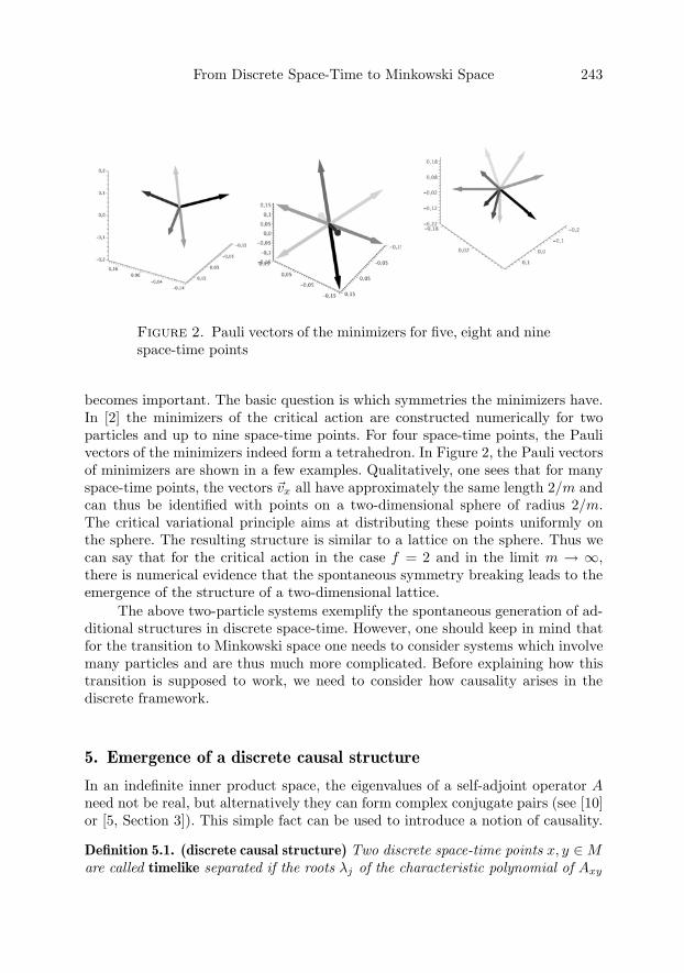
From Discrete Space-Time to Minkowski Space 243
Figure 2. Pauli vectors of the minimizers for five, eight and ninespace-time points
becomes important. The basic question is which symmetries the minimizers have.In [2] the minimizers of the critical action are constructed numerically for twoparticles and up to nine space-time points. For four space-time points, the Paulivectors of the minimizers indeed form a tetrahedron. In Figure 2, the Pauli vectorsof minimizers are shown in a few examples. Qualitatively, one sees that for manyspace-time points, the vectors �vx all have approximately the same length 2/m andcan thus be identified with points on a two-dimensional sphere of radius 2/m.The critical variational principle aims at distributing these points uniformly onthe sphere. The resulting structure is similar to a lattice on the sphere. Thus wecan say that for the critical action in the case f = 2 and in the limit m → ∞,there is numerical evidence that the spontaneous symmetry breaking leads to theemergence of the structure of a two-dimensional lattice.
The above two-particle systems exemplify the spontaneous generation of ad-ditional structures in discrete space-time. However, one should keep in mind thatfor the transition to Minkowski space one needs to consider systems which involvemany particles and are thus much more complicated. Before explaining how thistransition is supposed to work, we need to consider how causality arises in thediscrete framework.
5. Emergence of a discrete causal structure
In an indefinite inner product space, the eigenvalues of a self-adjoint operator Aneed not be real, but alternatively they can form complex conjugate pairs (see [10]or [5, Section 3]). This simple fact can be used to introduce a notion of causality.
Definition 5.1. (discrete causal structure) Two discrete space-time points x, y ∈Mare called timelike separated if the roots λj of the characteristic polynomial of Axy
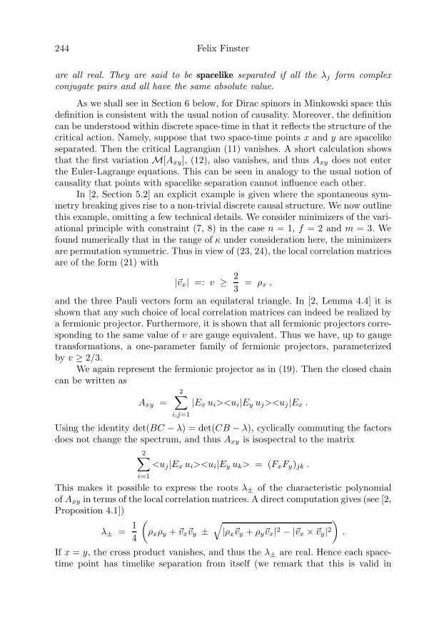
244 Felix Finster
are all real. They are said to be spacelike separated if all the λj form complexconjugate pairs and all have the same absolute value.
As we shall see in Section 6 below, for Dirac spinors in Minkowski space thisdefinition is consistent with the usual notion of causality. Moreover, the definitioncan be understood within discrete space-time in that it reflects the structure of thecritical action. Namely, suppose that two space-time points x and y are spacelikeseparated. Then the critical Lagrangian (11) vanishes. A short calculation showsthat the first variation M[Axy], (12), also vanishes, and thus Axy does not enterthe Euler-Lagrange equations. This can be seen in analogy to the usual notion ofcausality that points with spacelike separation cannot influence each other.
In [2, Section 5.2] an explicit example is given where the spontaneous sym-metry breaking gives rise to a non-trivial discrete causal structure. We now outlinethis example, omitting a few technical details. We consider minimizers of the vari-ational principle with constraint (7, 8) in the case n = 1, f = 2 and m = 3. Wefound numerically that in the range of κ under consideration here, the minimizersare permutation symmetric. Thus in view of (23, 24), the local correlation matricesare of the form (21) with
|�vx| =: v ≥ 23
= ρx ,
and the three Pauli vectors form an equilateral triangle. In [2, Lemma 4.4] it isshown that any such choice of local correlation matrices can indeed be realized bya fermionic projector. Furthermore, it is shown that all fermionic projectors corre-sponding to the same value of v are gauge equivalent. Thus we have, up to gaugetransformations, a one-parameter family of fermionic projectors, parameterizedby v ≥ 2/3.
We again represent the fermionic projector as in (19). Then the closed chaincan be written as
Axy =2∑
i,j=1
|Ex ui><ui|Ey uj><uj |Ex .
Using the identity det(BC − λ) = det(CB − λ), cyclically commuting the factorsdoes not change the spectrum, and thus Axy is isospectral to the matrix
2∑i=1
<uj|Ex ui><ui|Ey uk> = (FxFy)jk .
This makes it possible to express the roots λ± of the characteristic polynomialof Axy in terms of the local correlation matrices. A direct computation gives (see [2,Proposition 4.1])
λ± =14
(ρxρy + �vx�vy ±
√|ρx�vy + ρy�vx|2 − |�vx × �vy|2
).
If x = y, the cross product vanishes, and thus the λ± are real. Hence each space-time point has timelike separation from itself (we remark that this is valid in

From Discrete Space-Time to Minkowski Space 245
Figure 3. Plots of λ+ and λ− in the complex plane for varying v.
general, see [2, Proposition 2.7] and [5, Lemma 4.2]). In the case x �= y, theeigenvalues λ+ and λ− are shown in Figure 3 for different values of v. If v = 2/3,the eigenvalue λ− vanishes, whereas λ+ = 1/9. If v = 4
√3
9 , the values of λ−and λ+ coincide. If v is further increased, the λ± become complex and form acomplex conjugate pair. Hence different space-time points have timelike separationif v ≤ 4
√3
9 , whereas they have spacelike separation if v > 4√
39 . In the latter
case the discrete causal structure is non-trivial, because some pairs of points havespacelike and other pairs timelike separation. Finally, a direct computation of theconstraint (8) gives a relation between v and κ. One finds that v > 4
√3
9 if andonly if κ > 68
81 . We conclude that in the case κ > 6881 , the spontaneous symmetry
breaking leads to the emergence of non-trivial discrete causal structure.We point out that the discrete causal structure of Definition 5.1 differs from
the definition of a causal set (see [1]) in that it does not distinguish between futureand past directed separations. In the above example with three space-time points,the resulting discrete causal structure is also a causal set, albeit in a rather trivialway where each point has timelike separation only from itself.
6. A first connection to Minkowski space
In this section we describe how to get a simple connection between discrete space-time and Minkowski space. In the last Sections 7–9 we will proceed by explainingthe first steps towards making this intuitive picture precise. The simplest methodfor getting a correspondence to relativistic quantum mechanics in Minkowski spaceis to replace the discrete space-time points M by the space-time continuum R4 andthe sums over M by space-time integrals. For a vector Ψ ∈ H , the correspondinglocalization ExΨ should be a 4-component Dirac wave function, and the scalarproduct <Ψ(x) |Φ(x)> on Ex(H) should correspond to the usual Lorentz invariantscalar product on Dirac spinors ΨΦ with Ψ = Ψ†γ0 the adjoint spinor. Since this
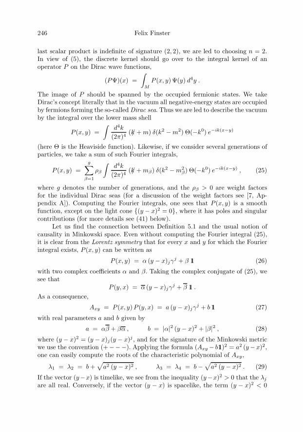
246 Felix Finster
last scalar product is indefinite of signature (2, 2), we are led to choosing n = 2.In view of (5), the discrete kernel should go over to the integral kernel of anoperator P on the Dirac wave functions,
(PΨ)(x) =∫
M
P (x, y)Ψ(y) d4y .
The image of P should be spanned by the occupied fermionic states. We takeDirac’s concept literally that in the vacuum all negative-energy states are occupiedby fermions forming the so-called Dirac sea. Thus we are led to describe the vacuumby the integral over the lower mass shell
P (x, y) =∫
d4k
(2π)4(k/ + m) δ(k2 −m2) Θ(−k0) e−ik(x−y)
(here Θ is the Heaviside function). Likewise, if we consider several generations ofparticles, we take a sum of such Fourier integrals,
P (x, y) =g∑
β=1
ρβ
∫d4k
(2π)4(k/ + mβ) δ(k2 −m2
β) Θ(−k0) e−ik(x−y) , (25)
where g denotes the number of generations, and the ρβ > 0 are weight factorsfor the individual Dirac seas (for a discussion of the weight factors see [7, Ap-pendix A]). Computing the Fourier integrals, one sees that P (x, y) is a smoothfunction, except on the light cone {(y − x)2 = 0}, where it has poles and singularcontributions (for more details see (41) below).
Let us find the connection between Definition 5.1 and the usual notion ofcausality in Minkowski space. Even without computing the Fourier integral (25),it is clear from the Lorentz symmetry that for every x and y for which the Fourierintegral exists, P (x, y) can be written as
P (x, y) = α (y − x)jγj + β 11 (26)
with two complex coefficients α and β. Taking the complex conjugate of (25), wesee that
P (y, x) = α (y − x)jγj + β 11 .
As a consequence,
Axy = P (x, y)P (y, x) = a (y − x)jγj + b 11 (27)
with real parameters a and b given by
a = αβ + βα , b = |α|2 (y − x)2 + |β|2 , (28)
where (y − x)2 = (y − x)j(y − x)j , and for the signature of the Minkowski metricwe use the convention (+−−−). Applying the formula (Axy − b11)2 = a2 (y−x)2,one can easily compute the roots of the characteristic polynomial of Axy,
λ1 = λ2 = b +√a2 (y − x)2 , λ3 = λ4 = b−
√a2 (y − x)2 . (29)
If the vector (y−x) is timelike, we see from the inequality (y−x)2 > 0 that the λj
are all real. Conversely, if the vector (y − x) is spacelike, the term (y − x)2 < 0
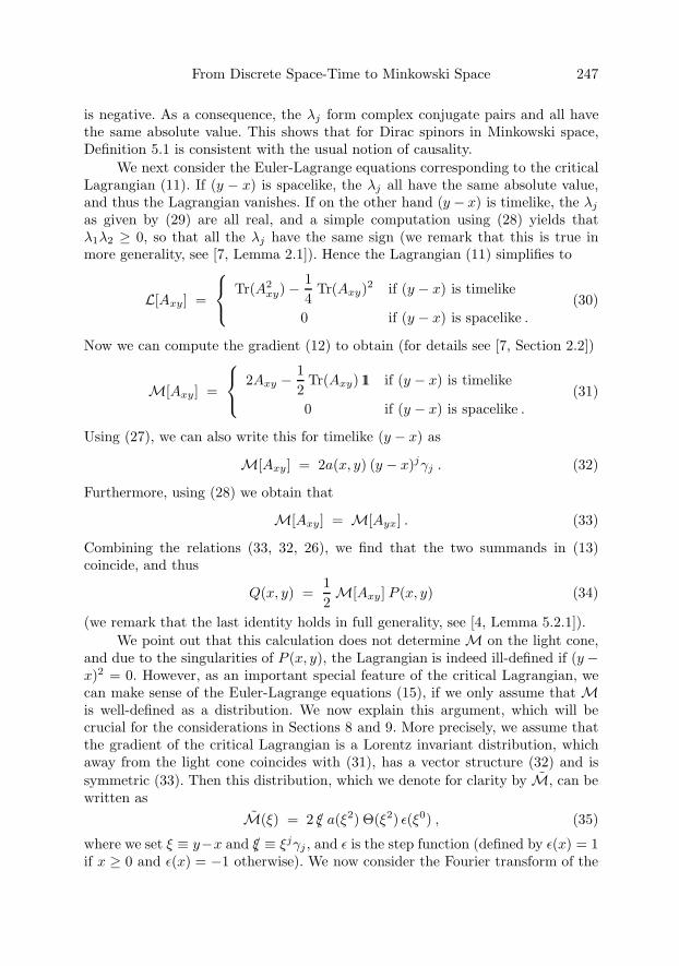
From Discrete Space-Time to Minkowski Space 247
is negative. As a consequence, the λj form complex conjugate pairs and all havethe same absolute value. This shows that for Dirac spinors in Minkowski space,Definition 5.1 is consistent with the usual notion of causality.
We next consider the Euler-Lagrange equations corresponding to the criticalLagrangian (11). If (y − x) is spacelike, the λj all have the same absolute value,and thus the Lagrangian vanishes. If on the other hand (y − x) is timelike, the λj
as given by (29) are all real, and a simple computation using (28) yields thatλ1λ2 ≥ 0, so that all the λj have the same sign (we remark that this is true inmore generality, see [7, Lemma 2.1]). Hence the Lagrangian (11) simplifies to
L[Axy] =
⎧⎨⎩ Tr(A2xy)− 1
4Tr(Axy)2 if (y − x) is timelike
0 if (y − x) is spacelike .(30)
Now we can compute the gradient (12) to obtain (for details see [7, Section 2.2])
M[Axy] =
⎧⎨⎩ 2Axy −12
Tr(Axy) 11 if (y − x) is timelike
0 if (y − x) is spacelike .(31)
Using (27), we can also write this for timelike (y − x) as
M[Axy] = 2a(x, y) (y − x)jγj . (32)
Furthermore, using (28) we obtain that
M[Axy] = M[Ayx] . (33)
Combining the relations (33, 32, 26), we find that the two summands in (13)coincide, and thus
Q(x, y) =12M[Axy] P (x, y) (34)
(we remark that the last identity holds in full generality, see [4, Lemma 5.2.1]).We point out that this calculation does not determine M on the light cone,
and due to the singularities of P (x, y), the Lagrangian is indeed ill-defined if (y−x)2 = 0. However, as an important special feature of the critical Lagrangian, wecan make sense of the Euler-Lagrange equations (15), if we only assume that Mis well-defined as a distribution. We now explain this argument, which will becrucial for the considerations in Sections 8 and 9. More precisely, we assume thatthe gradient of the critical Lagrangian is a Lorentz invariant distribution, whichaway from the light cone coincides with (31), has a vector structure (32) and issymmetric (33). Then this distribution, which we denote for clarity by M, can bewritten as
M(ξ) = 2 ξ/ a(ξ2) Θ(ξ2) ε(ξ0) , (35)
where we set ξ ≡ y−x and ξ/ ≡ ξjγj , and ε is the step function (defined by ε(x) = 1if x ≥ 0 and ε(x) = −1 otherwise). We now consider the Fourier transform of the
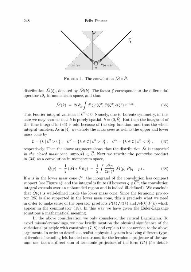
248 Felix Finster
p0
�p
qM(p) P (q − p)
Figure 4. The convolution M ∗ P .
distribution M(ξ), denoted by M(k). The factor ξ/ corresponds to the differentialoperator i∂/k in momentum space, and thus
M(k) = 2i ∂/k
∫d4ξ a(ξ2) Θ(ξ2) ε(ξ0) e−ikξ . (36)
This Fourier integral vanishes if k2 < 0. Namely, due to Lorentz symmetry, in thiscase we may assume that k is purely spatial, k = (0, �k). But then the integrand ofthe time integral in (36) is odd because of the step function, and thus the wholeintegral vanishes. As in [4], we denote the mass cone as well as the upper and lowermass cone by
C = {k | k2 > 0} , C∨ = {k ∈ C | k0 > 0} , C∧ = {k ∈ C | k0 < 0} , (37)
respectively. Then the above argument shows that the distribution M is supportedin the closed mass cone, suppM ⊂ C. Next we rewrite the pointwise productin (34) as a convolution in momentum space,
Q(q) =12
(M ∗ P )(q) =12
∫d4p
(2π)4M(p) P (q − p) . (38)
If q is in the lower mass cone C∧, the integrand of the convolution has compactsupport (see Figure 4), and the integral is finite (if however q �∈ C∧, the convolutionintegral extends over an unbounded region and is indeed ill-defined). We concludethat Q(q) is well-defined inside the lower mass cone. Since the fermionic projec-tor (25) is also supported in the lower mass cone, this is precisely what we needin order to make sense of the operator products P (k)M(k) and M(k) P (k) whichappear in the commutator (15). In this way we have given the Euler-Lagrangeequations a mathematical meaning.
In the above consideration we only considered the critical Lagrangian. Toavoid misunderstandings, we now briefly mention the physical significance of thevariational principle with constraint (7, 8) and explain the connection to the abovearguments. In order to describe a realistic physical system involving different typesof fermions including left-handed neutrinos, for the fermionic projector of the vac-uum one takes a direct sum of fermionic projectors of the form (25) (for details
From Discrete Space-Time to Minkowski Space 249
see [4, §5.1]). On the direct summands involving the neutrinos, the closed chain Axy
vanishes identically, and also the Euler-Lagrange equations are trivially satisfied.On all the other direct summands, we want the operator M to be of the form (35),so that the above considerations apply again. In order to arrange this, the valueof the Lagrange multiplier μ must be larger than the critical value 1
2n . Thus weare in the case μ > 1
2n where the auxiliary variational principle has no minimizers.This is why we need to consider the variational principle with constraint (7, 8).Hence the fermionic projector of fundamental physics should be a minimizer of thevariational principle with constraint (7, 8) corresponding to a value μ > 1
2n of theLagrange multiplier (such minimizers with μ > 1
2n indeed exist, see [2, Proposi-tion 5.2] for a simple example). The physical significance of the critical variationalprinciple lies in the fact that restricting attention to one direct summand of theform (25) (or more generally to a subsystem which does not involve chiral par-ticles), the Euler-Lagrange equations corresponding to (7, 8) coincide with thosefor the critical Lagrangian as discussed above. For more details we refer to [4,Chapter 5].
7. A static and isotropic lattice model
Our concept is that for many particles and many space-time points, the mech-anism explained in Sections 4 and 5 should lead to the spontaneous emergenceof the structure of Minkowski space or a Lorentzian manifold. The transition be-tween discrete space-time and the space-time continuum could be made precise byproving conjectures of the following type.
Conjecture 7.1. In spin dimension (2, 2), there is a series of fermion systems indiscrete space-time (H(l), <.|.>, (E(l)
x )x∈M(l) , P (l)) with the following properties:
(1) The fermionic projectors P (l) are minimizers of the auxiliary variational prin-ciple (9) in the critical case μ = 1
4 .(2) The number of space-time points m(l) and the number of particles f (l) scale
in l as follows,m(l) ∼ l4 , f (l) ∼ l3 .
(3) There are positive constants c(l), embeddings ι(l) : M (l) ↪→ R4 and isomor-phisms α(l) : H(l) → L2(Φ(l)(M (l)), <.|.>) (where <.|.> is the standardinner product on Dirac spinors <Φ|Ψ> = Φ†γ0Ψ), such that for any testwave functions Ψ,Φ ∈ C∞
0 (R4)4,
c(l)∑
x,y∈M(l)
Φ(ιx)†α(l)E(l)x P (l)E(l)
y (α(l))−1Ψ(ιy)
l→∞−→∫
d4x
∫d4y Φ(x)†P (x, y)Ψ(y) ,
where P (x, y) is the distribution (25).
250 Felix Finster
(4) As l →∞, the operators M[A(l)xy] converge likewise to the distribution M(ξ),
(35).
Similarly, one can formulate corresponding conjectures for systems involving sev-eral Dirac seas, where the variational principle (7) with constraint (8) should beused if chiral particles are involved. Moreover, it would be desirable to specify thatminimizers of the above form are in some sense generic. Ultimately, one wouldlike to prove that under suitable generic conditions, every sequence of minimizingfermion systems has a subsequence which converges in the above weak sense to aninteracting physical system defined on a Lorentzian manifold.
Proving such conjectures is certainly difficult. In preparation, it seems a goodidea to analyze particular aspects of the problem. One important task is to under-stand why discrete versions of Dirac sea configurations (25) minimize the criticalaction. A possible approach is to analyze discrete fermion systems numerically. Inorder to compare the results in a reasonable way to the continuum, one clearlyneeds systems involving many space-time points and many particles. Unfortu-nately, large discrete systems are difficult to analyze numerically. Therefore, itseems a good idea to begin the numerical analysis with simplified systems, whichcapture essential properties of the original system but are easier to handle. In [9]such a simplified system is proposed, where we employ a spherically symmetric andstatic Ansatz for the fermionic projector. We now briefly outline the derivation ofthis model and discuss a few results.
For the derivation we begin in Minkowski space with a static and isotropicsystem, which means that the fermionic projector P (x, y) depends only on thedifference ξ = y − x and is spherically symmetric. We take the Fourier transform,
P (ξ) =∫
d4p
(2π)4P (p) eipξ , (39)
and take for P an Ansatz involving a vector-scalar structure, i.e.
P (p) = vj(p) γj + φ(p) 11 (40)
with real functions vj and φ. Using the spherical symmetry, we can choose polarcoordinates and carry out the angular integrals in (39). This leaves us with a two-dimensional Fourier integral from the momentum variables (ω = p0, k = |�p|) to theposition variables (t = ξ0, r = |�ξ|). In order to discretize the system, we restrictthe position variables to a finite lattice L,
(t, r) ∈ L :={0, 2π, . . . , 2π(Nt − 1)
}×{0, 2π, . . . , 2π(Nr − 1)
}.
Here the integer parameters Nt and Nr describe the size of the lattice, and byscaling we arranged that the lattice spacing is equal to 2π. Then the momentumvariables are on the corresponding dual lattice L,
(ω, k) ∈ L :={− (Nt − 1), . . . ,−1, 0
}×{1, . . . , Nr
}.

From Discrete Space-Time to Minkowski Space 251
Figure 5. Action for a lattice system with two occupied states
Defining the closed chain by A(t, r) = P (t, r)P (t, r)∗, we can again introduce thecritical Lagrangian (10) with μ = 1
4 . For the action, we modify (9) to
S[P ] =∑
(t,r)∈L
ρt(t) ρr(r) L(t, r) ,
where the weight factors ρt and ρr take into account that we only consider positive tand that a point (t, r) corresponds to many states on a sphere of radius r. Whenvarying the action we need to take into account two constraints, called the tracecondition and the normalization condition, which take into account that the totalnumber of particles is fixed and that the fermionic projector should be idempotent.
In [9, Proposition 6.1] the existence of minimizers is proved, and we alsopresent first numerical results for a small lattice system. More precisely, we consideran 8 × 6-lattice and occupy one state with k = 1 and one with k = 2. Theabsolute minimum is attained when occupying the lattice points (ω1 = −1, k = 1)and (ω2 = −2, k = 2). Introducing a parameter τ by the requirement that thespatial component of the vector v in (40) should satisfy the relation |�v| = φ sinh τ ,the trace and normalization conditions fix our system up to the free parameters τ1and τ2 at the two occupied space-time points. In Figure 5 the action is shown asa function of these two free parameters. The minimum at the origin correspondsto the trivial configuration where the two vectors vi are both parallel to the ω-axis. However, this is only a local minimum, whereas the absolute minimum ofthe action is attained at the two non-trivial points (τ1 ≈ 1.5, τ2 ≈ 1) and (τ1 ≈−1.5, τ2 ≈ −1).
Obviously, a system of two occupied states on an 8 × 6-lattice is much toosmall for modeling a Dirac sea structure. But at least, our example shows thatour variational principle generates a non-trivial structure on the lattice where the
252 Felix Finster
occupied points distinguish specific lattice points, and the corresponding vectors vare not all parallel.
8. Analysis of regularization tails
Another important task in making the connection to Minkowski space rigorous isto justify the distribution M in (35). To explain the difficulty, let us assume that wehave a family of fermion systems (H(l), <.|.>, (E(l)
x )x∈M(l) , P (l)) having the prop-erties (1)-(3) of Conjecture 7.1. We can then regard the operators α(l)P (l)(α(l))−1
as regularizations of the continuum fermionic projector (25). It is easier to considermore generally a family of regularizations (P ε)ε>0 in Minkowski space with
P ε(x, y) ε↘0−→ P (x, y) in the distributional sense.
The parameter ε should be the length scale of the regularization. In order tojustify (35) as well as the convolution integral (38), our regularization should havethe following properties:
Definition 8.1. The fermionic projector satisfies the assumption of a distributionalMP -product if the following conditions are satisfied:
(i) There is a distribution M(ξ) of the form (35) such that limε↘0M[Aεxy] =
M(ξ) in the distributional sense.(ii) For every k for which limε↘0 Q
ε(k) exists, the convolution integral (38) iswell-defined and limε↘0 Q
ε(k) = Q(k).
This notion was introduced in [4, §5.6] and used as an ad-hoc assumption onthe regularization. Justifying this assumption is not just a technicality, but seemsessential for getting a detailed understanding of how the connection between dis-crete space-time and Minkowski space is supposed to work. Namely, if one takesa simple ultraviolet regularization (for example a cutoff in momentum space),then, due to the distributional singularity of P (x, y) on the light cone, the prod-uct Aε
xy = P ε(x, y)P ε(y, x) will in the limit ε↘ 0 develop singularities on the lightcone, which are ill-defined even in the distributional sense. Thus, in order to satisfythe conditions of Definition 8.1, we need to construct special regularizations, suchthat the divergences on the light cone cancel. In [7] it is shown that this can in-deed be accomplished. The method is to consider a class of spherically symmetricregularizations involving many free parameters, and to adjust these parameterssuch that all the divergences on the light cone and near the origin compensateeach other. It seems miraculous that it is possible to cancel all the divergencies;this can be regarded as a confirmation for our approach. If one believes that theregularized fermionic projector describes nature, we get concrete hints on how thevacuum should look like on the Planck scale. More specifically, the admissible reg-ularizations give rise to a multi-layer structure near the light cone involving severallength scales.

From Discrete Space-Time to Minkowski Space 253
In this survey article we cannot enter into the constructions of [7]. Instead,we describe a particular property of Dirac sea configurations which is crucial formaking the constructions work. Near the light cone, the distribution P (x, y) hasan expansion of the following form
P (x, y) = +iC0 ξ/PPξ4
+ C1PPξ2
+ iC2 ξ/PPξ2
+ C3 log(ξ2) + · · ·
+ε(ξ0)(D0 ξ/δ
′(ξ2) + iD1 δ(ξ2) + D2 ξ/δ(ξ2) + iD3 Θ(ξ2) + · · ·)
(41)
with real constants Cj and Dj (PP denotes the principal part; for more detailssee [7, Section 3]). Let us consider the expression M[Axy], (31), for timelike ξ.Computing the closed chain by Axy = P (x, y)P (x, y)∗, from (41) we obtain awayfrom the light cone the expansion
Axy =C2
0
ξ6+
C21 + 2C0C2
ξ4+ 2C0D3
ξ/ ε(ξ0)ξ4
+ · · · (ξ2 > 0). (42)
It is remarkable that there is no contribution proportional to ξ//ξ6. This is becausethe term ∼ C0C1 is imaginary, and because the contributions corresponding to D0,D1 and D2 are supported on the light cone. Taking the trace-free part, we find
M[Axy] = 4C0D3ξ/ ε(ξ0)ξ4
+ · · · (ξ2 > 0). (43)
The important point is that, due to the specific form of the Dirac sea configuration,the leading pole of M[Axy] on the light cone is of lower order than expected froma naive scaling. This fact is extremely useful in the constructions of [7]. Namely,if we consider regularizations of the distribution (41), the terms correspondingto C0, C1 and C2 will be “smeared out” and will thus no longer be supportedon the light cone. In particular, the contribution ∼ C0D1 no longer vanishes, andthis vector contribution can be used to modify (43). In simple terms, this effectmeans that the contributions by the regularization are amplified, making it possibleto modify M[Aε
xy] drastically by small regularization terms. In [7] we work withregularization tails, which are very small but spread out on a large scale εγ with γ <1. Taking many tails with different scales gives rise to the above-mentioned multi-layer structure. Another important effect is that the regularization yields bilinearcontributions to M[Aε
xy] of the form ∼ iC0D0γtγr (with γr = �ξ�γ/|�ξ|), which are
even more singular on the light cone than the vector contributions. The bilinearcontributions tend to make the roots λj complex (as can be understood alreadyfrom the fact that (iγtγr)2 = −11). This can be used to make a neighborhood ofthe light cone space-like; more precisely,
M[Aεxy] ≡ 0 if |ξ0| < |�ξ|+ εγ |�ξ|− 1
α with γ < 1 and α > 1. (44)
The analysis in [7] also specifies the singularities of the distribution M on thelight cone (recall that by (31), M is determined only away from the light cone).

254 Felix Finster
We find that M is unique up to the contributions
M(x, y) - c0 ξ/ δ′(ξ2) ε(ξ0) + c1 ξ/ δ(ξ2) ε(ξ0) (45)
with two free parameters c0, c1 ∈ R. Moreover, the regularization tails give usadditional freedom to modify M[Aε
xy] near the origin ξ = 0. This makes it possibleto go beyond the distributional MP -product by arranging extra contributionssupported at the origin. Expressed in momentum space, we may modify Q(q) bya polynomial in Q; namely (see [7, Theorem 2.4])
Q(q) := limε↘0
Qε(q) =12
(M ∗ P )(q) + c2 + c3 q/ + c4 q2 (q ∈ C∧) (46)
with additional free parameters c2, c3, c4 ∈ R.
9. A variational principle for the masses of the Dirac seas
With the analysis of the regularization tails in the previous section we have giventhe Euler-Lagrange equations for a vacuum Dirac sea configuration a rigorousmathematical meaning. All the formulas are well-defined in Minkowski space with-out any regularization. The freedom to choose the regularization of the fermionicprojector is reflected by the free real parameters c0, . . . , c4 in (45) and (46). Thisresult is the basis for a more detailed analysis of the Euler-Lagrange equations forvacuum Dirac sea configurations as carried out recently in [8]. We now outline themethods and results of this paper.
We first recall the notion of state stability as introduced in [4, §5.6]. We wantto analyze whether the vacuum Dirac sea configuration is a stable local minimumof the critical variational principle within the class of static and homogeneousfermionic projectors in Minkowski space. Thus we consider variations where wetake an occupied state of one of the Dirac seas and bring the corresponding particleto any other unoccupied state q ∈ Q∧. Taking into account the vector-scalarstructure in the Ansatz (25) and the negative definite signature of the fermionicstates, we are led to the variations (for details see [4, §5.6])
δP = −c(k/ + m) e−ik(x−y) + c(l/ + m) e−iq(x−y) (47)
with m ∈ {m1, . . . ,mg} � √q2, k2 = l2 = m2 and k0, l0 < 0. We demand that
such variations should not decrease the action,
S[P + δP ] ≥ S[P ] for all variations (47).
For the proper normalization of the fermionic states, we need to consider thesystem in finite 3-volume. Since the normalization constant c in (47) tends to zeroin the infinite volume limit, we may treat δS as a first order perturbation. Hencecomputing the variation of the action by (14), we obtain the condition stated inthe next definition. Note that, according to (45), (46) and (38), we already know

From Discrete Space-Time to Minkowski Space 255
that Q is well-defined inside the lower mass cone and has a vector scalar structure,i.e.
Q(k) = ak/
|k| + b , k ∈ C∧ , (48)
where we set |k| =√k2, and a = a(k2), b = b(k2) are two real-valued, Lorentz
invariant functions.
Definition 9.1. The fermionic projector of the vacuum is called state stable if thefunctions a and b in the representation (48) of Q(k) have the following properties:(1) a is non-negative.(2) The function a + b is minimal on the mass shells,
(a + b)(m2α) = inf
q∈C∧(a + b)(q2) for all α ∈ {1, . . . , g}. (49)
It is very helpful for the understanding and the analysis of state stabilitythat the condition (49) can be related to the Euler-Lagrange equations of a cor-responding variational principle. This variational principle was introduced in [8]for unregularized Dirac sea configurations of the form (25) and can be regardedas a Lorentz invariant analog of the critical variational principle. To define thisvariational principle, we expand the trace-free part of the closed chain inside thelight cone similar to (41, 42) as follows,
A0(ξ) := Axy −14
Tr(Axy) = ξ/ ε(ξ0)(
m3
ξ4+
m5
ξ2+O(log ξ2)
),
where the coefficients m3 and m5 are functions of the parameters ρβ and mβ in (25).Using the simplified form (30) of the critical Lagrangian, we thus obtain for ξ inthe interior of the light cone the expansion
L = Tr(A0(ξ)2) =m3
ξ6+
2m3m5
ξ4+O(ξ−2 log ξ2) (ξ2 > 0).
The naive adaptation of the critical action (9) would be to integrate L over theset {ξ2 > 0} (for details see [8, Section 2]). However, this integral diverges becausethe hyperbolas {ξ2 = const}, where L is constant, have infinite measure. To avoidthis problem, we introduce the variable z = ξ2 and consider instead the one-dimensional integral
∫∞0L(z) z dz, which has the same dimension of length as the
integral∫L d4ξ. Since this new integral is still divergent near z = 0, we subtract
suitable counter terms and set
S = limε↘0
(∫ ∞
ε
L(z) z dz − m23
ε+ 2 m3 m5 log ε
). (50)
In order to build in the free parameters c0, c1 in (45) and c2, c3 in (46), we introducethe extended action by adding extra terms,
Sext = S + F (m3,m5) + c3
g∑β=1
ρβ m4β + c4
g∑β=1
ρβ m5β , (51)

256 Felix Finster
0 5 10 15 20 25q
282 800
282 900
283 000
283 100
283 200
�a�b��q2�
Figure 6. A state stable Dirac sea structure with three generations
where F is an arbitrary real function (note that the parameter c2 in (46) is ir-relevant for state stability because it merely changes the function b in (48) by aconstant). In our Lorentz invariant variational principle we minimize (51), varyingthe parameters ρβ and mβ under the constraint
g∑β=1
mβ ρ3β = const .
This constraint is needed to rule out trivial minimizers; it can be understood asreplacing the condition in discrete space-time that the number of particles is fixed.
In [8] it is shown that, allowing for an additional “test Dirac sea” of massmg+1 and weight ρg+1 (with ρg+1 = 0 but δρg+1 �= 0), the corresponding Euler-Lagrange equations coincide with (49). The difficult point in the derivation isto take the Fourier transform of the Lorentz invariant action and to reformulatethe ε-regularization in (50) in momentum space. In [8] we proceed by constructingnumerical solutions of the Euler-Lagrange equations which in addition satisfy thecondition (1) in Definition 9.1. We thus obtain state stable Dirac sea configurations.Figure 6 shows an example with three generations and corresponding values of theparameters m1 = 1, m2 = 5, m3 = 20 and ρ1 = 1, ρ2 = 10−4, ρ3 = 9.696× 10⁻⁶.
10. The continuum limit
The continuum limit provides a method for analyzing the Euler-Lagrange equa-tions (15) for interacting systems in Minkowski space. For details and results werefer to [4, Chapters 6-8]; here we merely put the procedure of the continuum limitin the context of the methods outlined in Sections 6–9. As explained in Section 8,the regularization yields bilinear contributions to Aε
xy, which make a neighbor-hood of the light cone spacelike (44). Hence near the light cone, the roots λj of
From Discrete Space-Time to Minkowski Space 257
the characteristic polynomial form complex conjugate pairs and all have the sameabsolute value,
|λi| = |λj | for all i, j, (52)so that the critical Lagrangian (11) vanishes identically. If we introduce an interac-tion (for example an additional Dirac wave function or a classical gauge field), thecorresponding perturbation of the fermionic projector will violate (52). We thusobtain corresponding contributions to M[Aε
xy] in a strip of size ∼ ε around thelight cone. These contributions diverge if the regularization is removed. For small ε,they are much larger than the contributions by the regularization tails as discussedin Section 8; this can be understood from the fact that they are much closer tothe light cone. The formalism of the continuum limit is obtained by an expansionof these divergent contributions in powers of the regularization length ε. The de-pendence of the expansion coefficients on the regularization is analyzed using themethod of variable regularization; we find that this dependence can be describedby a small number of free parameters, which take into account the unknown struc-ture of space-time on the Planck scale. The dependence on the gauge fields can beanalyzed explicitly using the method of integration along characteristics or, moresystematically, by performing a light-cone expansion of the fermionic projector. Inthis way, one can relate the Euler-Lagrange equations to an effective interactionin the framework of second quantized Dirac fields and classical bosonic fields.
11. Outlook and open problems
In this paper we gave a detailed picture of the transition from discrete space-timeto the usual space-time continuum. Certain aspects have already been workedout rigorously. But clearly many questions are still open. Generally speaking, themain task for making the connection between discrete space-time and Minkowskispace rigorous is to clarify the symmetries and the discrete causal structure ofthe minimizers for discrete systems involving many particles and many space-timepoints. More specifically, we see the following directions for future work:
1. Numerics for large lattice models: The most direct method to clarify the con-nection between discrete and continuous models is to the static and isotropiclattice model [9] for systems which are so large that they can be comparedin a reasonable way to the continuum. Important questions are whether theminimizers correspond to Dirac sea configurations and what the resultingdiscrete causal structure is. The next step will be to analyze the connectionto the regularization effects described in [7]. In particular, does the latticemodel give rise to a multi-layer structure near the light cone? What are theresulting values of the constants c0, . . . , c4 in (45, 46)?
2. Numerics for fermion systems in discrete space-time: For more than twoparticles, almost nothing is known about the minimizers of our variationalprinciples. A systematic numerical study could answer the question whetherfor many particles and many space-time points, the minimizers have outer
258 Felix Finster
symmetries which can be associated to an underlying lattice structure. Anumerical analysis of fermion systems in discrete space-time could also justifythe spherically symmetric and static Ansatz in [9].
3. Analysis and estimates for discrete systems: In the critical case, the generalexistence problem for minimizers is still open. Furthermore, using methodsof [6], one can study fermion systems with prescribed outer symmetry analyt-ically. One question of interest is whether for minimizers the discrete causalstructure is compatible with the structure of a corresponding causal set. Itwould be extremely useful to have a method for analyzing the minimizersasymptotically for a large number of space-time points and many particles.As a first step, a good approximation technique (maybe using methods fromquantum statistics?) would be very helpful.
4. Analysis of the Lorentz invariant variational principle: In [8] the variationalprinciple for the masses of the vacuum Dirac seas is introduced and analyzed.However, the existence theory has not yet been developed. Furthermore, thestructure of the minimizers still needs to be worked out systematically.
5. Analysis of the continuum limit: It is a major task to analyze the continuumlimit in more detail. The next steps are the derivation of the field equationsand the analysis of the spontaneous symmetry breaking of the chiral gaugegroup. Furthermore, except for [3, Appendix B], no calculations for gravita-tional fields have been made so far. The analysis of the continuum limit shouldalso give constraints for the weight factors ρβ in (25) (see [8, Appendix A]).
6. Field quantization: As explained in [4, §3.6], the field quantization effectsshould be a consequence of a “discreteness” of the interaction described byour variational principle. This effect could be studied and made precise forsmall discrete systems.
Apart from being a challenge for mathematics, these problems have the physicalperspective of clarifying the microscopic structure of our universe and explainingthe emergence of space and time.
References
[1] L. Bombelli, J. Lee, D. Meyer, R. Sorkin, “Space-time as a causal set,” Phys. Rev.Lett. 59 (1987) 521-524
[2] A. Diethert, F. Finster, D. Schiefeneder, “Fermion systems in discrete space-timeexemplifying the spontaneous generation of a causal structure,” arXiv:0710.4420[math-ph] (2007)
[3] F. Finster, “Light-cone expansion of the Dirac sea to first order in the externalpotential,” hep-th/9707128, Michigan Math. J. 46 (1999) 377-408
[4] F. Finster, “The Principle of the Fermionic Projector,” AMS/IP Studies in AdvancedMathematics 35 (2006)
[5] F. Finster, “A variational principle in discrete space-time – existence of minimizers,”math-ph/0503069, Calc. Var. and Partial Diff. Eq. 29 (2007) 431-453

From Discrete Space-Time to Minkowski Space 259
[6] F. Finster, “Fermion systems in discrete space-time – outer symmetries and spon-taneous symmetry breaking,” math-ph/0601039, Adv. Theor. Math. Phys. 11 (2007)91-146
[7] F. Finster, “On the regularized fermionic projector of the vacuum,” math-ph/0612003v2, to appear in J. Math. Phys. (2008)
[8] F. Finster, S. Hoch, “An action principle for the masses of Dirac particles,”arXiv:0712.0678 [math-ph] (2007)
[9] F. Finster, W. Plaum, “A lattice model for the fermionic projector in a static andisotropic space-time,” arXiv:0712.0676 [math-ph], to appear in Math. Nachr. (2008)
[10] I. Gohberg, P. Lancaster, L. Rodman, “Matrices and Indefinite Scalar Products,”Birkhauser Verlag (1983)
Felix FinsterNWF I – MathematikUniversitat RegensburgD–93040 Regensburge-mail: [email protected]


Quantum Field TheoryB. Fauser, J. Tolksdorf and E. Zeidler, Eds., 261–283c© 2009 Birkhauser Verlag Basel/Switzerland
Towards a q-Deformed Quantum Field Theory
Hartmut Wachter
In memory of Julius Wess.
Abstract. The formalism of q-deformation seems to enable the formulation ofphysical theories on discrete spacetime structures that do not suffer from theabsence of well-known spacetime symmetries. In this manner q-deformationcan lead to a new regularization mechanism in quantum field theory andrequires a substantial revision of the mathematical formalism quantum theoryis based on. The article gives a review of the motivation for q-deformationin physics, describes the main ideas of the new formalism and outlines thecurrent status of its application to quantum theory.
Mathematics Subject Classification (2000). Primary 81R50; Secondary 16W30;17B37.
Keywords. q-deformation, quantum groups, quantum spaces, q-deformed freeSchrodinger particle, q-calculus.
1. Introduction
I would like to start with some historical notes. From the great mathematicianBernhard Riemann we know that the answer to the question for the right geometryof spacetime is essential to physics. The founders of modern quantum theory, i.e.people like Bohr, Born, Dirac, or Heisenberg were of the opinion that the deeperreason for the infinities in quantum field theory lies in an inadequate description ofthe geometry of spacetime at very small distances. They believed that spacetimeitself had to be incorporated into a quantization scheme. On these grounds itis not very astonishing that the idea of quantizing spacetime is nearly as old asmodern quantum theory itself [1,2]. Up to the present day many researchers tookup this idea over and over again [3–8] (for a survey see, for example, Ref. [9]) buttheir approaches often suffer from conceptual difficulties such as the breakdown ofLorentz symmetry or the prediction of new, rather unusual phenomena.

262 Hartmut Wachter
Feynman, Schwinger, and Tomonaga suggested a different method to over-come the difficulties with infinities in quantum field theory. Their approach isknown as renormalization theory [10–12]. With the great experimental success ofrenormalization theory after the Second World War most efforts towards quantiz-ing spacetime came to an end. Although theoreticians at first felt rather uncom-fortable with renormalization theory they began to accept it since it gave them atool at hand by which they could make numerical predictions that were in aston-ishing agreement with experiment. Nowadays the ideas of renormalization theoryare well understood and much progress in quantum field theory was due to theassumption that any sensible physical theory should be renormalizable.
Nevertheless, theoreticians are convinced that renormalizable theories areonly a low-energy approximation to a more fundamental, possibly non-renormaliza-ble theory. This belief is nourished by the following observation. Renormalizabilityallows us to neglect certain quantum processes yielding divergent diagrams in aperturbative treatment. The reason for this lies in the fact that such quantumprocesses should be highly suppressed at accessible energies. They only have aninfluence on the masses and charges that are actually measured. However, whenquantum corrections to the gravitational field become important these assumptionsseem no longer acceptable. This claim is underpinned by the continued failure tofind a renormalizable theory of gravitation.
As renormalizability seems to be not a fundamental physical requirement, theold idea of quantizing spacetime enjoys a revival. In this respect, quantum groupsand quantum spaces that arise from q-deformation provide a suitable frameworkfor formulating physical theories on quantized spaces [13–23]. They imply dis-cretizations of well-known spacetime structures [24–29], which, in turn, lead to avery powerful regularization mechanism, as is demonstrated in Sec. 2 of this article.
The attractiveness of q-deformed quantum groups and quantum spaces stemsfrom the fact that they describe discrete spaces that do not suffer from the ab-sence of the well-known spacetime symmetries. However, there is a high price wehave to pay for this feature, since the usage of quantum groups and quantumspaces requires a complete revision of the mathematics important physical ideasare formulated by. In Sec. 3 we show how the elements of analysis like partialderivatives, integrals, and so on change under q-deformation. On the other handthe mathematics of q-deformed quantum groups and quantum spaces is sophisti-cated enough to ensure that well-established physical laws pertain. The treatmentof the free non-relativistic q-deformed particle underlines this statement as will beseen in section 4.
2. q-Regularization
In this section we would like to illustrate the regularization mechanism inducedby q-deformation. First of all, let us recall that quantizing spacetime can singleout a lattice which, in turn, implies the existence of a smallest length given by the

Towards a q-Deformed Quantum Field Theory 263
lattice spacing. On such a discrete spacetime plane-waves of wave-length smallerthan twice the lattice spacing could not propagate. Since wave-length and mo-mentum of a plane-wave are inversely proportional to each other it then followsthat momentum space would be bounded. As a consequence all integrals over loopmomenta should take on finite values.
As we will see below, q-deformation realizes these general ideas in a moresubtle way. To this end, let us consider the following q-analogs of trigonometricalfunctions [30]:
cosq(x) ≡∞∑
k =0
(−1)kx2k
[2k]q!, sinq(x) ≡ q1/2
∞∑k =0
(−1)kx2k+1
[2k + 1]q!. (2.1)
The symmetrical q-numbers and their factorials are respectively given by [31]
[n]q ≡qn − q−n
q − q−1, q > 1, (2.2)
and[n]q! ≡ [n]q [n− 1]q . . . [1]q, [0]q! ≡ 1. (2.3)
From Fig. 1 we see that the q-trigonometrical functions are more or less pe-riodic, but their maxima and minima increase in height exponentially.
32.521.510.50
5
2.5
0
-2.5
-5
x
y
x
y
Figure 1. Fig. 1: Plot of the q-trigonometrical functioncosq(x/(q − q−1)), section at q = 1.1
The q-regularization mechanism is based on the following very remarkableproperty of q-trigonometrical functions [32, 33]: There are real constants a and bsuch that
limn→∞ cosq(aq2n) = lim
n→∞ sinq(bq2n+1) = 0. (2.4)

264 Hartmut Wachter
If the q-trigonometrical functions are given by the expressions in (2.1) these con-stants take on the values
a =q−1/2
q − q−1, b =
q1/2
q − q−1. (2.5)
The deeper reason for this behavior of q-trigonometrical functions lies in thefact that their sequence of roots approach the values aq2n or bq2n+1 if n tendsto infinity. Table 1 contains the absolute values of cosq(aq2n) one obtains when nruns through all integers from 1 to 20. A short glance at the table tells us thatthey are decreasing very rapidly with increasing n (notice that the smallest valuesappear in the top line and the biggest ones in the bottom line).
Tab. 1: The absolute values of cosq(aq2n) for n = 1, . . . , 20, q = 1.1
1.0954837827, 0.3806453606, 1.3002562658, 0.7466139278,0.2073439674, 0.0332735098, 0.0033145196, 0.0002126316,8.97256×10-6, 2.52305×10⁻⁷, 4.76707×10⁻⁹, 6.08464×10⁻¹¹,
5.26538×10⁻¹³, 3.09651×10⁻¹⁵, 1.23955×10⁻¹⁷, 3.38126×10-20,6.28977×10-23, 7.98276×10⁻²⁶, 6.91482×10⁻²⁹, 4.08903×10⁻³².
In complete analogy to the undeformed case the q-trigonometrical functionsin (2.1) represent the real and imaginary part of q-deformed plane-waves. Transi-tion amplitudes in a q-deformed quantum field theory are then given by Fouriertransforms that are formulated by means of q-trigonometrical functions and so-called Jackson integrals. The latter are given by [34]∫ ∞
0
dqx f(x) ≡∞∑
k =−∞(q − 1)(c qk)f(c qk), (2.6)
where c stands for an undetermined real constant. In this manner, the followingexpressions are viewed as q-analogs of one-dimensional Fourier transforms:∫ ∞
0
dq2x f(x) · cosq(x p) ≡∞∑
k =−∞(q2 − 1) (aq2k) f(aq2k) · cosq(aq2kp), (2.7)
∫ ∞
0
dq2x f(x) · sinq(x p) ≡∞∑
k =−∞(q2 − 1) (bq2k+1) f(bq2k+1) · sinq(bq2k+1p).
(2.8)
Notice that in (2.7) and (2.8) we set c equal to a and b, respectively [cf. Eq. (2.5)].Essential for us is the following observation. If we require that the value of the
momentum variable p takes on even powers of q, the sums on the right-hand sideof (2.7) and (2.8) even converge for functions f(x) that have no classical Fouriertransform. To illustrate this point let us turn our attention to the expression∫ ∞
a
dq2xx10 · cosq(x) =∞∑
k = 0
(q2 − 1) (a11q22k) · cosq(aq2k). (2.9)
Towards a q-Deformed Quantum Field Theory 265
It is part of the calculation of a q-deformed Fourier transform of the functionf(x) = x10. Table 2 contains the numerical values of all partial sums of the Jacksonintegral in (2.9) that contain no more than twenty summands. Once again, we seethat their sequence converges so fast that we are allowed to truncate the sum in(2.9) after twenty summations. It should finally be mentioned that this observationis a consequence of the property in (2.4).
Tab. 2: Partial sums with no more than twenty summands , q = 1.1
8.57483×10⁷, 2.96844×10⁸, -5.03939×10⁹, 1.76356×10¹⁰,-2.89647×10¹⁰, 2.63758×10¹⁰, -1.44196×10¹⁰, 4.94746×10⁹,-1.10037×10⁹, 1.58134×10⁸, -1.78318×10⁷, -1.21080×10⁶,-2.27518×10⁶, -2.22886×10⁶, -2.23023×10⁶, -2.23021×10⁶,-2.23021×10⁶, -2.23021×10⁶, -2.23021×10⁶, -2.23021×10⁶.
The considerations so far should now enable us to understand the regular-ization mechanism in a q-deformed field theory. It can be described as follows:The Jackson integral is determined by the values its integrand takes on for thepoints c q2n or c q2n+1, where n ∈ Z. These points establish a so-called q-latticewith offset c. A suitable choice for c guarantees that the values of the q-deformedtrigonometrical functions rapidly diminish on the q-lattice points with increasingdistance from the origin. This feature carries over to the integrands of q-deformedFourier integrals and so insures their convergency.
3. Basic ideas of the mathematical formalism
This section is devoted to mathematical ideas which are indispensable for under-standing q-deformed versions of physical theories. The presentation gives a briefoutline of the subject, only. In this respect, it shall serve as a kind of ’appetizer’.For details, we refer the reader to Refs. [35–42].
3.1. What are quantum groups and quantum spaces?
Let us first recall that spacetime symmetries are normally described by Lie groups.Roughly speaking, quantum groups are nothing other than natural generalizationsof such groups. To understand this assertion in more detail let us also recall thata group G is a set on which an associative product is defined such that a unitelement e exists and such that every element u has an inverse u−1. Instead ofworking with the group elements itself, it is possible to restrict attention to linearfunctions on the group. The latter constitute an algebra which is often denotedby F(G). One finds that the group multiplication induces on F(G) an algebraicstructure making F(G) into a so-called Hopf algebra. To each group we can con-struct a Hopf algebra but the converse does not hold in general, since the varietyof Hopf algebras is larger than that of groups. Quantum groups, for example, areHopf algebras, but they show a non-commutative algebraic structure that preventsus from identifying them with an algebra of linear functions on an ordinary group.

266 Hartmut Wachter
�
�
� �
acts on co-acts on
is dual to
is dual to
V
g
F(V )
F(g)
Figure 2. Relation between a group g and its function algebra F(g)
Nevertheless, quantum groups show features that are reminiscent of function al-gebras on a group. In this sense, it should become clear that quantum groups canbe viewed as generalizations of groups.
Perhaps, the reader may have realized that the notion of a quantum grouparises from a process of dualization in which the group structure is replaced bya Hopf structure. There is a similar relationship between ordinary spaces andquantum spaces. To this end let us recall that a physical space such as a coordinatespace is often described as a vector space V some group G acts upon. In otherwords, physical spaces are representations of their symmetry groups and are oftenreferred to as modules. Interestingly, the vector space F(V ) being dual to a givenmodule V contains the same information as the module itself. In mathematicalterms, this observation amounts to the assertion that F(V ) becomes a so-calledco-representation or co-module of F(G) (see Fig. 2).
Quantum spaces are generalizations of ordinary spaces insofar as they are de-fined as co-modules of quantum groups. In this respect, they are non-commutativespaces whose symmetry is governed by quantum groups. To sum up, dualizing thenotion of a group and that of its representations we arrive at generalizations ofordinary physical spaces and their symmetries.
The simplest example of a quantum space is given by the famous Maninplane, which is spanned by the coordinates X1 and X2 subject to
X1X2 = qX2X1, q > 1. (3.1)
The Manin plane is a co-representation of the quantum group SLq(2). The latter isa Hopf algebra generated by four non-commuting elements which we can arrange

Towards a q-Deformed Quantum Field Theory 267
in matrix form:
M ij =
(a bc d
). (3.2)
If we do so, the coactions of SLq(2) on quantum plane coordinates become
β(X i) = M ij ⊗Xj . (3.3)
The requirement of covariance, i.e.
β(X1)β(X2) = qβ(X2)β(X1), (3.4)
implies the relations
ab = qba, ac = qca, bc = cb, bd = qdb,
cd = qdc, ad− da = (q − q−1)bc. (3.5)
3.2. How do we multiply on quantum spaces?
From the example in the last subsection we saw that quantum spaces are spannedby non-commuting elements. The essential feature of our approach is that we real-ize the non-commutative structure of our quantum space algebras on commutativecoordinate spaces. To achieve this, we make use of the fact that there are vectorspace isomorphisms that map normal ordered monomials of the non-commutingquantum space generators to the corresponding monomials of ordinary coordinates,i.e.
W−1 : Vq −→ V,
W−1((X1)i1 . . . (Xn)in) ≡ (x1)i1 . . . (xn)in . (3.6)
Notice that we denote quantum space generators by capital letters. It should alsobe clear that the vector space isomorphism W is completely determined by (3.6),since each quantum space element can be written as a formal power series ofnormal ordered monomials.
Interestingly, one can extend the above vector space isomorphism to an al-gebra isomorphism by introducing a non-commutative product in V , the so-calledstar product [43–45]. This product is defined via the relation
W(f � g) = W(f) · W(g), (3.7)
being tantamount tof � g ≡ W−1 (W (f) · W (g)) , (3.8)
where f and g are formal power series in the commutative coordinate algebra V .In the case of the Manin plane, for example, the star product can be calculated
from the operator expression
f(xi) � g(xj) = [ q−nx2 ny1 f(xi) g(yj)]y→x
= f(xi) g(xj) + O(h), with h = ln q, (3.9)
where we introduced the operators
nxi ≡ xi ∂
∂xi, i = 1, 2. (3.10)

268 Hartmut Wachter
The second equality in (3.9) tells us that the star product modifies the commutativeproduct by terms depending on h = ln q. Evidently, this modifications vanish inthe classical limit q → 1.
3.3. What are q-deformed translations?
Translations in spacetime play a very important role in physics as the fundamentalphysical laws have to be invariant under translations. From a mathematical pointof view, translations are described by a mapping (We use alternatively X ∼= X⊗1and Y ∼= 1⊗X)
Δ : Vq → Vq ⊗ Vq, (3.11)with
Δ(X i) ≡ [X i](1) ⊗ [X i](2) = X i ⊗ 1 + 1⊗X i = X i + Y i. (3.12)
The expressions Δ(X i), i = 1, . . . , n, are the components of a vector obtainedfrom two other vectors with components X i and Y i via vector addition. For thisreason the vector components Δ(X i) should obey the same algebraic propertiesas the quantum space coordinates X i. Concretely, we require
Δ(X iZj) = Δ(X i)Δ(Zj), Δ(β(X i)) = β(Δ(X i)), (3.13)
i.e. the mapping in (3.11) has to be a co-module algebra homomorphism.The first relation in (3.13) implies that the components Δ(X i) again fulfil the
commutation relations between quantum space coordinates. The second relation in(3.13) tells us that the components Δ(X i) behave under symmetry transformationsin very much the same way as quantum space coordinates X i.
However, to satisfy the requirements in (3.13) we have to introduce a non-commutative tensor product by
(1⊗X i) · (Xj ⊗ 1) = kRijkl X
k ⊗X l, k ∈ R, (3.14)
or, alternatively, by
(1⊗X i) · (Xj ⊗ 1) = k−1(R−1)ijkl X
k ⊗X l, (3.15)
where R denotes the so-called R-matrix of the quantum space under consideration.It should be clear that for ordinary spaces the R-matrix and its inverse degenerateto the twist matrix δi
kδjl .
In principle, we have everything together to calculate translations of mono-mials of quantum space generators. This can be achieved in the following manner:
Δ((X1)i1 . . . (Xn)in) = ((Δ(X1))i1 . . . (Δ(Xn))in)
= (X1 ⊗ 1 + 1⊗X1)i1 . . . (Xn ⊗ 1 + 1⊗Xn)in
= [(X1)i1 . . . (Xn)in ](1) ⊗ [(X1)i1 . . . (Xn)in ](2). (3.16)
The first step is the homomorphism property of Δ and the second step makesuse of (3.12). For the last step we have to apply (3.14) and end up with a kindof binomial theorem. Instead of (3.14) we could also work with (3.15). Doing sowould lead us to a second q-analog of the binomial theorem.

Towards a q-Deformed Quantum Field Theory 269
In the case of Manin plane these considerations yield, for example,
Δ((X1)n1(X2)n2) =n1∑
k1=0
n2∑k2=0
q−(n1− k1)k2
[n1
k1
]q−2
[n2
k2
]q−2
× (X1)k1(X2)k2 ⊗ (X1)n1− k1(X2)n2− k2 , (3.17)
where the q-deformed binomial coefficients are defined in analogy to their unde-formed counterparts:[
α
m
]qb
≡[[α]]qb [[α− 1]]qb . . . [[α−m + 1]]qb
[[m]]qb !, b ∈ C,m ∈ N. (3.18)
If we want to deal with inverse translations we need a further mapping givenby
S : Vq → Vq, S(X i) ≡ −X i. (3.19)This mapping is an anti-algebra homomorphism. The values of S on monomialsare determined in such a way that it holds
m◦ (1⊗S)◦Δ((X1)i1 . . . (Xn)in) = m◦ (S⊗1)◦Δ((X1)i1 . . . (Xn)in) = 0. (3.20)
Without going into the details, it should be mentioned that the operations in(3.11), (3.14), (3.15), and (3.19) again have realizations on commutative coordinatespaces. For these realizations we introduce the following notation:
Δ → f(xi ⊕A yj), S → f(.A xi),
(1⊗ a) · (b⊗ 1) → f(xi)x|y/A g(yj). (3.21)
Notice that we have two different versions of each of the above operations accordingto the two possible choices for the non-commutative tensor product [cf. Eqs. (3.14)and (3.15)]. To distinguish them we introduced the label A ∈ {L, L}.
It should also be mentioned that q-translations fulfil some interesting calcula-tional rules. In terms of the operations on the commutative spaces they take a formthat is strongly reminiscent of the group axioms satisfied by ordinary translations.We wish to illustrate this statement by the identities
f((xi ⊕A yj)⊕ (.A yk)) = f(xi ⊕A (yj ⊕ (.A yk)))
= f(xi ⊕A 0) = f(xi). (3.22)
The first equality in (3.22) means associativity of q-deformed translations and thesecond equality concerns the existence of inverse elements.
Finally, we would like to point out for the mathematically oriented readerthat q-deformed translations are connected with braided Hopf algebras [46, 47].In this respect, the equalities in (3.22) follow from the axioms of a braided Hopfalgebra.

270 Hartmut Wachter
3.4. How to differentiate and integrate on quantum spaces
Partial derivatives on quantum spaces should generate infinitesimal q-translations.In this sense, we can introduce q-deformed partial derivatives by
∂i f(xj) ≡ limyk→0
f(yk ⊕L xj)− f(xj)yi
,
∂i f(xj) ≡ limyk→0
f(yk ⊕L xj)− f(xj)yi
, (3.23)
f(xj) ! ∂i ≡ limyk→0
f(xj)− f(xj ⊕L yk)yi
,
f(xj) ! ∂i ≡ limyk→0
f(xj)− f(xj ⊕L yk)yi
. (3.24)
The symbols , , !, and ! denote left and right actions. Objects with lower andupper indices transform into each other via a quantum metric (for the details, seeRef. [48]).
There are operator representations for the action of partial derivatives. Theycan be read off from the operator expressions for q-deformed translations, sincewe have
f(xi ⊕L yj) = 1⊗ f(yj) + xk ⊗ ∂k f(yj) + O(x2),
f(xi ⊕L yj) = 1⊗ f(yj) + xk ⊗ ∂k f(yj) + O(x2), (3.25)
f(yi ⊕L xj) = f(yi)⊗ 1− f(yi) ! ∂k ⊗ xk + O(x2),
f(yi ⊕L xj) = f(yi)⊗ 1− f(yi) ! ∂k ⊗ xk + O(x2), (3.26)
where repeated indices are to be summed over.As representations of partial derivatives on the Manin plane we obtain, for
example,
∂1 f(x1, x2) = D1q2f(x1, q2x2),
∂2 f(x1, x2) = D2q2f(qx1, x2). (3.27)
In the above formulae we introduced the so-called Jackson derivatives [49], whichare given by
Diqaf(xi) ≡ f(qaxi)− f(xi)
(qa − 1)xi. (3.28)
Being difference operators the Jackson derivatives represent discretized versions ofordinary derivatives.
Next, we come to integrals on quantum spaces. They can be seen as operationsbeing inverse to partial derivatives. More concretely, an integral gives a solutionto the equation
∂i F = f, (3.29)
Towards a q-Deformed Quantum Field Theory 271
where f is a given function. The following reasonings about calculating integralsapply to all types of partial derivatives introduced in (3.23) and (3.24).
To find solutions to Eq. (3.29) it is helpful to realize that the operator ex-pressions for partial derivatives on quantum spaces split into a classical part ∂i
cl
and corrections ∂icor vanishing in the undeformed limit q → 1, i.e.
∂i F =(∂icl + ∂i
cor
) F. (3.30)
The classical part is always invertible, so we have
F = (∂i)−1 f =1
∂icl + ∂i
cor
f
=1
∂icl
(1 + (∂i
cl)−1∂icor
) f =1
1 + (∂icl)−1∂i
cor
· 1∂icl
f
=∞∑
k=0
(−1)k [(∂icl)
−1∂icor
]k(∂i
cl)−1 f. (3.31)
Once again, we wish to demonstrate our considerations by a simple example.Comparing the expressions in (3.27) with the right-hand side of Eq. (3.30) we findthat
(∂1)cl f = D1q2f(q2x2), (∂1)cor f = 0,
(∂2)cl f = D2q2f(qx1), (∂2)cor f = 0, (3.32)
which, in turn, leads to
(∂1)−1 f = (∂1)−1cl f = (D1
q2)−1f(q−2x2),
(∂2)−1 f = (∂2)−1cl f = (D2
q2)−1f(q−1x1), (3.33)
where (Diqa)−1 denotes the Jackson integral operator[cf. Eq. (2.6)].
Partial derivatives and integrals on quantum spaces lead us into the realmof multi-dimensional q-analysis. This subject was completely worked out in Ref.[41], where we derived various calculational rules such as Leibniz rules for partialderivatives, rules for integration by parts or q-analogs of the fundamental theoremof calculus.
3.5. Fourier transformations on quantum spaces
Fourier transformations play a very important role in quantum physics. Thus, itarises the question what are Fourier transformations on quantum spaces. To an-swer this question we first introduce q-analogs of plane-waves. In complete analogyto the undeformed case they are defined to be eigenfunctions of q-deformed partialderivatives [38,50,51]. Notice that q-deformed partial derivatives can act in differ-ent ways on a function and for this reason there are different versions of q-deformed
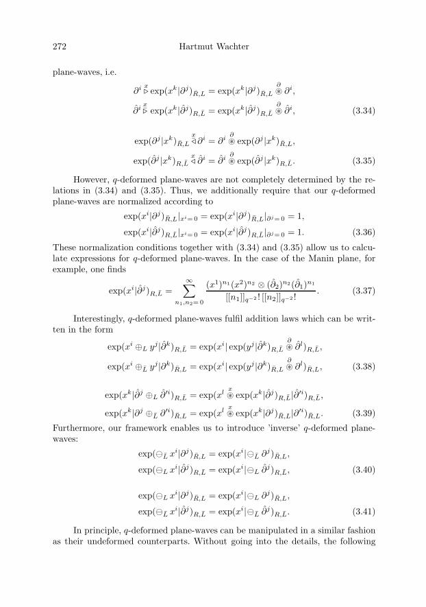
272 Hartmut Wachter
plane-waves, i.e.
∂i x exp(xk|∂j)R,L = exp(xk|∂j)R,L
∂� ∂i,
∂ix exp(xk|∂j)R,L = exp(xk|∂j)R,L
∂� ∂i, (3.34)
exp(∂j |xk)R,L
x! ∂i = ∂i
∂� exp(∂j |xk)R,L,
exp(∂j |xk)R,L
x! ∂i = ∂i
∂� exp(∂j |xk)R,L. (3.35)
However, q-deformed plane-waves are not completely determined by the re-lations in (3.34) and (3.35). Thus, we additionally require that our q-deformedplane-waves are normalized according to
exp(xi|∂j)R,L|xi=0 = exp(xi|∂j)R,L|∂j=0 = 1,
exp(xi|∂j)R,L|xi=0 = exp(xi|∂j)R,L|∂j=0 = 1. (3.36)
These normalization conditions together with (3.34) and (3.35) allow us to calcu-late expressions for q-deformed plane-waves. In the case of the Manin plane, forexample, one finds
exp(xi|∂j)R,L =∞∑
n1,n2= 0
(x1)n1(x2)n2 ⊗ (∂2)n2(∂1)n1
[[n1]]q−2 ! [[n2]]q−2 !. (3.37)
Interestingly, q-deformed plane-waves fulfil addition laws which can be writ-ten in the form
exp(xi ⊕L yj|∂k)R,L = exp(xi| exp(yj |∂k)R,L
∂� ∂l)R,L,
exp(xi ⊕L yj|∂k)R,L = exp(xi| exp(yj |∂k)R,L
∂� ∂l)R,L, (3.38)
exp(xk|∂j ⊕L ∂′i)R,L = exp(xlx� exp(xk|∂j)R,L|∂′i)R,L,
exp(xk|∂j ⊕L ∂′i)R,L = exp(xlx� exp(xk|∂j)R,L|∂′i)R,L. (3.39)
Furthermore, our framework enables us to introduce ’inverse’ q-deformed plane-waves:
exp(.L xi|∂j)R,L = exp(xi|.L ∂j)R,L,
exp(.L xi|∂j)R,L = exp(xi|.L ∂j)R,L, (3.40)
exp(.L xi|∂j)R,L = exp(xi|.L ∂j)R,L,
exp(.L xi|∂j)R,L = exp(xi|.L ∂j)R,L. (3.41)
In principle, q-deformed plane-waves can be manipulated in a similar fashionas their undeformed counterparts. Without going into the details, the following

Towards a q-Deformed Quantum Field Theory 273
calculation shall serve as an example:
exp(xi|x� exp(.L xj |∂k)R,L
∂� ∂l)R,L = exp(xi ⊕L (.L xj)|∂k)R,L
= exp(xi|∂l)R,L|xi=0 = 1. (3.42)
It should be obvious that the above result justifies to identify the expressions in(3.40) and (3.41) with inverse q-deformed plane-waves.
Now, we have everything together to introduce Fourier transformations onquantum spaces. Due to the different versions of q-deformed plane-waves, thereare the following possibilities for defining Fourier transformations on quantumspaces [52, 53]:
FL(f)(pk) ≡∫ +∞
−∞dn1x f(xi)
x� exp(xj |i−1pk)R,L,
FL(f)(pk) ≡∫ +∞
−∞dn2x f(xi)
x� exp(xj |i−1pk)R,L, (3.43)
FR(f)(pk) ≡∫ +∞
−∞dn1x exp(i−1pk|xj)R,L
x� f(xi),
FR(f)(pk) ≡∫ +∞
−∞dn2x exp(i−1pk|xj)R,L
x� f(xi). (3.44)
Let us make some comments on these definitions. First of all, we appliedthe substitution ∂k = i−1pk to our q-deformed plane-waves. The integrals over thewhole space are obtained by applying one-dimensional integrals in succession. Thevolume elements of the integrals carry an index which is a consequence of the factthat we have two q-deformed differential calculi.
There is a second set of q-deformed Fourier transformations. They are givenby
F∗L(f)(xk) ≡ 1
vol1
∫ +∞
−∞dn1p exp(i−1pl|.L xk)R,L
x|p/ L f(pj),
F ∗L(f)(xk) ≡ 1
vol2
∫ +∞
−∞dn2p exp(i−1pl|.L xk)R,L
x|p/L f(pj), (3.45)
F∗R(f)(xk) ≡ 1
vol2
∫ +∞
−∞dn2p f(pj)
p|x/R exp(.R xk|i−1pl)R,L,
F ∗R(f)(xk) ≡ 1
vol1
∫ +∞
−∞dn1p f(pj)
p|x/R exp(.R xk|i−1pl)R,L. (3.46)
Notice that we introduced some sort of normalization constants (volα)−1, α ∈{1, 2}. They are determined in such a way that the Fourier transforms in (3.45)

274 Hartmut Wachter
and (3.46) are inverse to those in (3.43) and (3.44). To be more specific, we have
(F ∗R ◦ FL)(f)(xk) = f(κxk), (FL ◦ F ∗
R)(f)(xk) = κ−nf(κ−1xk),
(F∗R ◦ FL)(f)(xk) = f(κ−1xk), (FL ◦ F∗
R)(f)(xk) = κnf(κxk), (3.47)
(F ∗L ◦ FR)(f)(xk) = f(κ−1xk), (FR ◦ F ∗
L)(f)(xk) = κnf(κxk),
(F∗L ◦ FR)(f)(xk) = f(κxk), (FR ◦ F∗
L)(f)(xk) = κ−nf(κ−1xk), (3.48)
where κ denotes a certain constant.From the undeformed case we know that taking the Fourier transform of unity
yields a delta function. In this manner, q-analogs of the delta function should begiven by
δn1 (pk) ≡ FL(1)(pk) =
∫ +∞
−∞dn1x exp(xj |i−1pk)R,L,
δn2 (pk) ≡ FL(1)(pk) =
∫ +∞
−∞dn2x exp(xj |i−1pk)R,L. (3.49)
In analogy to their undeformed counterparts q-deformed delta functions fulfilas characteristic properties∫ +∞
−∞dn
αy f(yi)y� δn
β (yj ⊕C (.C xk)) = volα,β f(κ−1C xk), (3.50)
and ∫ +∞
−∞dn
αy δnβ ((.C xk)⊕C yj)
y� f(yi) = volα,β f(κ−1
C xk), (3.51)
where
volα,β ≡∫ +∞
−∞dn
αx δnβ (xk), α, β ∈ {1, 2}, (3.52)
andκL = κR = κ, κL = κR = κ−1. (3.53)
Moreover, one can show that the Fourier transform of a q-deformed delta functionyields a q-deformed plane-wave and vice versa.
Finally, let us mention that q-deformed Fourier transformations interchangethe star-product with q-deformed differentiation. The following identities shallserve as example:
FL(fx! ∂j)(pk) = FL(f)(pk)
p� (i−1pj),
FL(fx� xj)(pk) = FL(f)(pk)
p! (i∂j). (3.54)
4. Applications to physics
In the last section we gave a short introduction into analysis on q-deformed quan-tum spaces. It is now our aim to show how the new formalism applies to the
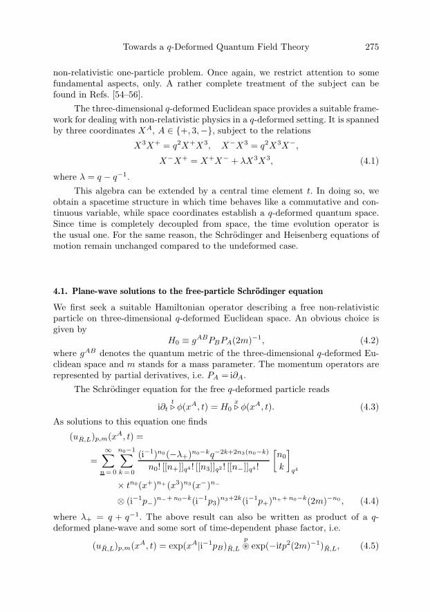
Towards a q-Deformed Quantum Field Theory 275
non-relativistic one-particle problem. Once again, we restrict attention to somefundamental aspects, only. A rather complete treatment of the subject can befound in Refs. [54–56].
The three-dimensional q-deformed Euclidean space provides a suitable frame-work for dealing with non-relativistic physics in a q-deformed setting. It is spannedby three coordinates XA, A ∈ {+, 3,−}, subject to the relations
X3X+ = q2X+X3, X−X3 = q2X3X−,
X−X+ = X+X− + λX3X3, (4.1)
where λ = q − q−1.
This algebra can be extended by a central time element t. In doing so, weobtain a spacetime structure in which time behaves like a commutative and con-tinuous variable, while space coordinates establish a q-deformed quantum space.Since time is completely decoupled from space, the time evolution operator isthe usual one. For the same reason, the Schrodinger and Heisenberg equations ofmotion remain unchanged compared to the undeformed case.
4.1. Plane-wave solutions to the free-particle Schrodinger equation
We first seek a suitable Hamiltonian operator describing a free non-relativisticparticle on three-dimensional q-deformed Euclidean space. An obvious choice isgiven by
H0 ≡ gABPBPA(2m)−1, (4.2)where gAB denotes the quantum metric of the three-dimensional q-deformed Eu-clidean space and m stands for a mass parameter. The momentum operators arerepresented by partial derivatives, i.e. PA = i∂A.
The Schrodinger equation for the free q-deformed particle reads
i∂tt φ(xA, t) = H0
x φ(xA, t). (4.3)
As solutions to this equation one finds
(uR,L)p,m(xA, t) =
=∞∑
n = 0
n0−1∑k = 0
(i−1)n0(−λ+)n0−kq−2k+2n3(n0−k)
n0! [[n+]]q4 ! [[n3]]q2 ! [[n−]]q4 !
[n0
k
]q4
× tn0(x+)n+(x3)n3(x−)n−
⊗ (i−1p−)n−+ n0−k(i−1p3)n3+2k(i−1p+)n++ n0−k(2m)−n0 , (4.4)
where λ+ = q + q−1. The above result can also be written as product of a q-deformed plane-wave and some sort of time-dependent phase factor, i.e.
(uR,L)p,m(xA, t) = exp(xA|i−1pB)R,L
p� exp(−itp2(2m)−1)R,L, (4.5)

276 Hartmut Wachter
with
exp(−itp2(2m)−1)R,L ≡∞∑
n =0
(−it)n
n!
n∑k=0
q−2k(−λ+)n−k
[n
k
]q4
× (p−)n−k(p3)2k(p+)n−k(2m)−n. (4.6)
Our solutions to the Schrodinger equation of the free q-deformed particlecan be regarded as q-analogs of momentum eigenfunctions of definite energy. Thisobservation follows from the identities
PAx (uR,L)p,m(xA, t) = i∂A
x (uR,L)p,m(xA, t)
= (uR,L)p,m(xA, t)p� pA, (4.7)
H0x (uR,L)p,m(xA, t) = (2m)−1P 2 x
(uR,L)p,m(xA, t)
= (uR,L)p,m(xA, t)p� p2(2m)−1. (4.8)
The above relations tell us that the wave function (uR,L)p,m corresponds to aparticle with momentum components pA, A ∈ {+, 3,−}, and energy
E = p2(2m)−1 = gABpB
p� pA(2m)−1. (4.9)
In complete analogy to the undeformed case, the time-evolution of our q-deformed momentum eigenfunctions is given by
(uR,L)p,m(xA, t) = exp(−itH0)H0|x exp(xA|i−1pB)R,L, (4.10)
i.e. we simply have to apply the usual time-evolution operator to a q-deformedplane-wave of three-dimensional q-deformed Euclidean space. It is not very difficultto check that (4.10) indeed gives a solution to the Schrodinger equation of the freeq-deformed particle. To this end, one inserts the expression in (4.10) into Eq. (4.3)and then applies the time derivative to the time evolution operator.
Our q-analogs of momentum eigenfunctions are normalized to q-deformeddelta functions. In this manner, they establish an orthonormal set of functions.Concretely, we have∫ +∞
−∞d31x (uR,L)�Lp,m(xA,−q−ζt)
p|x/ L (uR,L)p,m(xB , t) =
= (vol1)−1 δ31((.L pC)⊕L pD), (4.11)
with
vol1 ≡∫ +∞
−∞d31x
∫ +∞
−∞d31p exp(xA|i−1pB)R,L. (4.12)
It should be mentioned that the tensor multiplication /L on the left-hand side ofEq. (4.11) is due to the fact that q-deformed momentum eigenfunctions live in thetensor product of a position space with a momentum space.

Towards a q-Deformed Quantum Field Theory 277
Our q-deformed momentum eigenfunctions also fulfil a completeness relation.It reads ∫ +∞
−∞d31p (uR,L)p,m(xA, t)
p|y/L (uR,L)�Lp,m(yB ,−q−ζt) =
= (vol1)−1 δ31(x
A ⊕L (.L yB)). (4.13)
Notice that the time variable of the momentum eigenfunction with negative mo-mentum is affected by a scaling. This scaling ensures that the completeness rela-tion for q-deformed momentum eigenfunctions is time-independent. For the samereason the orthonormality relation in Eq. (4.11) does not vary with time.
Now, we are in a position to write down expressions for q-deformed wavepackets. As usual, they arise from superposition of q-deformed momentum eigen-functions. In this manner, we have
(φ∗1)m(xi) = (vol1)1/2
∫ +∞
−∞d31p (uR,L)p,m(xi)
p� (c∗1)κ−1p. (4.14)
The reader should not be confused about the different labels like the asterisk, sincetheir meaning is not important in this context. The volume integral in Eq. (4.14) isa q-deformed one and for the sake of simplicity we took the convention xi ≡ (xA, t).
Conversely, the completeness relations for q-deformed momentum eigenfunc-tions together with the properties of q-deformed delta functions allow us to regainthe expansion coefficients (c∗1)p from the wave packet (φ∗
1)m. This can be achievedby means of the formula
(c∗1)p =1
(vol1)1/2
∫ +∞
−∞d31x (uR,L)�Lp,m(xA,−q−ζt)
p|x/ L (φ∗
1)m(xi). (4.15)
The q-deformed wave-packets are again solutions to the free-particle Schro-dinger equation in (4.3), i.e.
i∂tt (φ∗
1)m(xi) = H0x (φ∗
1)m(xi). (4.16)
This observation is a direct consequence of the fact that a q-deformed wave-packetis a superposition of q-deformed momentum eigenfunctions. For the same reasonEq. (4.10) implies that
(φ∗1)m(xA, t) = exp(−itH0)
H0|x (φ∗
1)m(xA, t = 0). (4.17)
4.2. The propagator of the free q-deformed particle
Once the wave function of a quantum system is known at a certain time thetime-evolution operator enables us to find the wave function at any later time.However, there is another way to solve the time-evolution problem. It requires toknow the so-called propagator. It is now our aim to discuss the propagator of thefree non-relativistic q-deformed particle.
To this end, we insert the expression for the expansion coefficients givenby Eq. (4.15) into the expansion in Eq. (4.14). In doing so, we obtain an integral
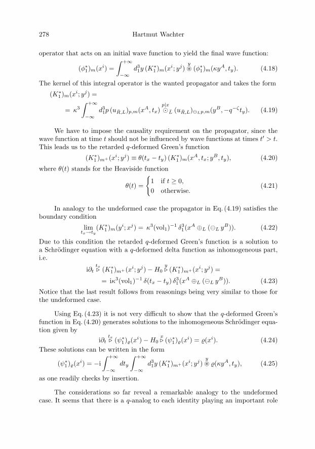
278 Hartmut Wachter
operator that acts on an initial wave function to yield the final wave function:
(φ∗1)m(xi) =
∫ +∞
−∞d31y (K∗
1 )m(xi; yj)y� (φ∗
1)m(κyA, ty). (4.18)
The kernel of this integral operator is the wanted propagator and takes the form
(K∗1 )m(xi; yj) =
= κ3
∫ +∞
−∞d31p (uR,L)p,m(xA, tx)
p|x/ L (uR,L)�Lp,m(yB,−q−ζty). (4.19)
We have to impose the causality requirement on the propagator, since thewave function at time t should not be influenced by wave functions at times t′ > t.This leads us to the retarded q-deformed Green’s function
(K∗1 )m+(xi; yj) ≡ θ(tx − ty) (K∗
1 )m(xA, tx; yB, ty), (4.20)
where θ(t) stands for the Heaviside function
θ(t) =
{1 if t ≥ 0,0 otherwise.
(4.21)
In analogy to the undeformed case the propagator in Eq. (4.19) satisfies theboundary condition
limtx→ty
(K∗1 )m(yi;xj) = κ3(vol1)−1 δ3
1(xA ⊕L (.L yB)). (4.22)
Due to this condition the retarded q-deformed Green’s function is a solution toa Schrodinger equation with a q-deformed delta function as inhomogeneous part,i.e.
i∂ttx (K∗
1 )m+(xi; yj)−H0y (K∗
1 )m+(xi; yj) =
= iκ3(vol1)−1 δ(tx − ty) δ31(xA ⊕L (.L yB)). (4.23)
Notice that the last result follows from reasonings being very similar to those forthe undeformed case.
Using Eq. (4.23) it is not very difficult to show that the q-deformed Green’sfunction in Eq. (4.20) generates solutions to the inhomogeneous Schrodinger equa-tion given by
i∂ttx (ψ∗
1)�(xi)−H0x (ψ∗
1)�(xi) = �(xi). (4.24)These solutions can be written in the form
(ψ∗1)�(xi) = −i
∫ +∞
−∞dty
∫ +∞
−∞d31y (K∗
1 )m+(xi; yj)y� �(κyA, ty), (4.25)
as one readily checks by insertion.
The considerations so far reveal a remarkable analogy to the undeformedcase. It seems that there is a q-analog to each identity playing an important role
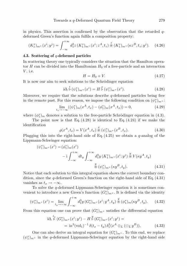
Towards a q-Deformed Quantum Field Theory 279
in physics. This assertion is confirmed by the observation that the retarded q-deformed Green’s function again fulfils a composition property:
(K∗1 )m+(xi; yj) =
∫ +∞
−∞d31z (K∗
1 )m+(xi; zA, tz)z� (K∗
1 )m+(κzB, tz; yj). (4.26)
4.3. Scattering of q-deformed particles
In scattering theory one typically considers the situation that the Hamilton opera-tor H can be divided into the Hamiltonian H0 of a free-particle and an interactionV , i.e.
H = H0 + V. (4.27)It is now our aim to seek solutions to the Schrodinger equation
i∂tt (ψ∗
1)m+(xi) = Hx (ψ∗
1)m+(xi). (4.28)
Moreover, we require that the solutions describe q-deformed particles being freein the remote past. For this reason, we impose the following condition on (ψ∗
1)m+ :
limtx→−∞((ψ∗
1)m(xA, tx)− (φ∗1)m(xA, tx)) = 0, (4.29)
where (φ∗1)m denotes a solution to the free-particle Schrodinger equation in (4.3).
The point now is that Eq. (4.28) is identical to Eq. (4.24) if we make theidentification
�(xA, tx) = V (xA, tx)x� (ψ∗
1)m+(xB, tx). (4.30)Plugging this into the right-hand side of Eq. (4.25) we obtain a q-analog of theLippmann-Schwinger equation:
(ψ∗1)m+(xi) = (φ∗
1)m(xi)
− i∫ +∞
−∞dty
∫ +∞
−∞d31y (K∗
1 )m+(xi; yj)y� V (κyA, ty)
y� (ψ∗
1)m+(κyB, ty). (4.31)
Notice that each solution to this integral equation shows the correct boundary con-dition, since the q-deformed Green’s function on the right-hand side of Eq. (4.31)vanishes as tx → −∞.
To solve the q-deformed Lippmann-Schwinger equation it is sometimes con-venient to introduce a new Green’s function (G∗
1)m+ . It is defined via the identity
(ψ∗1)m+(xi) = lim
ty→−∞
∫ +∞
−∞d31y (G∗
1)m+(xi; yA, ty)y� (φ∗
1)m(κyB, ty). (4.32)
From this equation one can prove that (G∗1)m+ satisfies the differential equation
i∂t
ty
(G∗1)m+(xi; yj)−H
y (G∗
1)m+(xi; yj) =
= iκ3(vol1)−1 δ(tx − ty) δ31(xA ⊕L (.L yB)), (4.33)
One can also derive an integral equation for (G∗1)m+ . To this end, we replace
(ψ∗1)m+ in the q-deformed Lippmann-Schwinger equation by the right-hand side
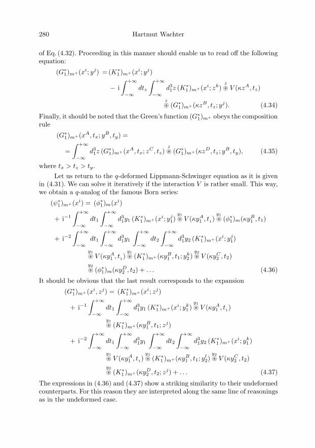
280 Hartmut Wachter
of Eq. (4.32). Proceeding in this manner should enable us to read off the followingequation:
(G∗1)m+(xi; yj) = (K∗
1 )m+(xi; yj)
− i∫ +∞
−∞dtz
∫ +∞
−∞d31z (K∗
1 )m+(xi; zk)z� V (κzA, tz)
z� (G∗
1)m+(κzB, tz; yj). (4.34)
Finally, it should be noted that the Green’s function (G∗1)m+ obeys the composition
rule
(G∗1)m+(xA, tx; yB, ty) =
=∫ +∞
−∞d31z (G∗
1)m+(xA, tx; zC , tz)z� (G∗
1)m+(κzD, tz ; yB, ty), (4.35)
where tx > tz > ty.Let us return to the q-deformed Lippmann-Schwinger equation as it is given
in (4.31). We can solve it iteratively if the interaction V is rather small. This way,we obtain a q-analog of the famous Born series:
(ψ∗1)m+(xi) = (φ∗
1)m(xi)
+ i−1
∫ +∞
−∞dt1
∫ +∞
−∞d31y1 (K∗
1 )m+(xi; yj1)
y1� V (κyA
1 , t1)y1� (φ∗
1)m(κyB1 , t1)
+ i−2
∫ +∞
−∞dt1
∫ +∞
−∞d31y1
∫ +∞
−∞dt2
∫ +∞
−∞d31y2 (K∗
1 )m+(xi; yj1)
y1� V (κyA1 , t1)
y1� (K∗1 )m+(κyB
1 , t1; yk2 )
y2� V (κyC2 , t2)
y2� (φ∗
1)m(κyD2 , t2) + . . . (4.36)
It should be obvious that the last result corresponds to the expansion
(G∗1)m+(xi, zj) = (K∗
1 )m+(xi; zj)
+ i−1
∫ +∞
−∞dt1
∫ +∞
−∞d31y1 (K∗
1 )m+(xi; yk1 )
y1� V (κyA
1 , t1)
y1� (K∗
1 )m+(κyB1 , t1; zj)
+ i−2
∫ +∞
−∞dt1
∫ +∞
−∞d31y1
∫ +∞
−∞dt2
∫ +∞
−∞d31y2 (K∗
1 )m+(xi; yk1 )
y1� V (κyA1 , t1)
y1� (K∗1 )m+(κyB
1 , t1; yl2)
y2� V (κyC2 , t2)
y2� (K∗
1 )m+(κyD2 , t2; zj) + . . . (4.37)
The expressions in (4.36) and (4.37) show a striking similarity to their undeformedcounterparts. For this reason they are interpreted along the same line of reasoningsas in the undeformed case.
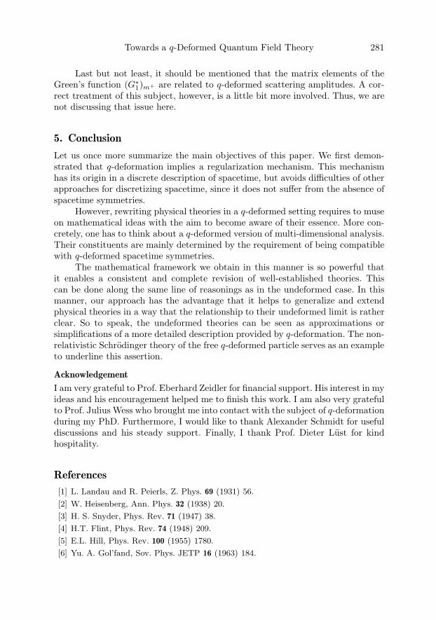
Towards a q-Deformed Quantum Field Theory 281
Last but not least, it should be mentioned that the matrix elements of theGreen’s function (G∗
1)m+ are related to q-deformed scattering amplitudes. A cor-rect treatment of this subject, however, is a little bit more involved. Thus, we arenot discussing that issue here.
5. Conclusion
Let us once more summarize the main objectives of this paper. We first demon-strated that q-deformation implies a regularization mechanism. This mechanismhas its origin in a discrete description of spacetime, but avoids difficulties of otherapproaches for discretizing spacetime, since it does not suffer from the absence ofspacetime symmetries.
However, rewriting physical theories in a q-deformed setting requires to museon mathematical ideas with the aim to become aware of their essence. More con-cretely, one has to think about a q-deformed version of multi-dimensional analysis.Their constituents are mainly determined by the requirement of being compatiblewith q-deformed spacetime symmetries.
The mathematical framework we obtain in this manner is so powerful thatit enables a consistent and complete revision of well-established theories. Thiscan be done along the same line of reasonings as in the undeformed case. In thismanner, our approach has the advantage that it helps to generalize and extendphysical theories in a way that the relationship to their undeformed limit is ratherclear. So to speak, the undeformed theories can be seen as approximations orsimplifications of a more detailed description provided by q-deformation. The non-relativistic Schrodinger theory of the free q-deformed particle serves as an exampleto underline this assertion.
Acknowledgement
I am very grateful to Prof. Eberhard Zeidler for financial support. His interest in myideas and his encouragement helped me to finish this work. I am also very gratefulto Prof. Julius Wess who brought me into contact with the subject of q-deformationduring my PhD. Furthermore, I would like to thank Alexander Schmidt for usefuldiscussions and his steady support. Finally, I thank Prof. Dieter Lust for kindhospitality.
References
[1] L. Landau and R. Peierls, Z. Phys. 69 (1931) 56.
[2] W. Heisenberg, Ann. Phys. 32 (1938) 20.
[3] H. S. Snyder, Phys. Rev. 71 (1947) 38.
[4] H.T. Flint, Phys. Rev. 74 (1948) 209.
[5] E.L. Hill, Phys. Rev. 100 (1955) 1780.
[6] Yu. A. Gol’fand, Sov. Phys. JETP 16 (1963) 184.

282 Hartmut Wachter
[7] D. Finkelstein, Int. J. Theor. Phys. 28 (1989) 441.
[8] C.J. Isham, in H. Lee, ed., Proceedings of the Advanced Summer Institute on Physics,Geometry and Topology, Plenum, New York (1990).
[9] E. Prugovecki, Principles of Quantum General Relativity, World Scientific, Singa-pore, 1995.
[10] S. Tomonaga, Prog. Theor. Phys. 1 (1946) 27; Phys. Rev. 74 (1948) 224.
[11] J. Schwinger, Phys. Rev. 75 (1949) 651; Phys. Rev. 76 (1949) 790.
[12] R.P. Feynman, Phys. Rev. 76 (1949) 749.
[13] P.P. Kulish and N. Yu. Reshetikin, J. Sov. Math. 23 (1983) 2345.
[14] V.G. Drinfeld, Sov. Math. Dokl. 32 (1985) 254.
[15] M. Jimbo, Lett. Math. Phys. 10 (1985) 63.
[16] V.G. Drinfeld, in A.M. Gleason, ed., Proceedings of the International Congress ofMathematicians, Amer. Math. Soc. (1986).
[17] Yu. I. Manin, Quantum Groups and Non-Commutative Geometry, Centre deRecherche Mathematiques, Montreal (1988).
[18] S.L. Woronowicz, Commun. Math. Phys. 111 (1987) 613.
[19] M. Takeuchi, Israel J. Math. 72 (1990) 232.
[20] N. Yu. Reshetikhin, L.A. Takhtadzhyan and L.D. Faddeev, Leningrad Math. J. 1(1990) 193.
[21] J. Wess and B. Zumino, Nucl. Phys. B. Suppl. 18 (1991) 302.
[22] S. Majid, Foundations of Quantum Group Theory, University Press, Cambridge(1995).
[23] M. Chaichian and A.P. Demichev, Introduction to Quantum Groups, World Scientific,Singapore, 1996.
[24] M. Fichtenmuller, A. Lorek and J. Wess, Z. Phys. C 71 (1996) 533, [hep-th/9511106].
[25] J. Wess, Int. J. Mod. Phys. A 12 (1997) 4997.
[26] B.L. Cerchiai and J. Wess, Eur. Phys. J. C 5 (1998) 553, [math.qa/9801104].
[27] H. Grosse, C. Klimcik and P. Presnajder, Int. J. Theor. Phys. 35 (1996) 231, [hep-th/9505175].
[28] S. Majid, Int. J. Mod. Phys. A 5 (1990) 4689.
[29] R. Oeckl, Commun. Math. Phys. 217 (2001) 451.
[30] T.H. Koornwinder, R.F. Swarttouw, Trans. AMS 333, 445 (1992).
[31] V. Kac and P. Cheung, Quantum Calculus, Springer-Verlag, Berlin (2000).
[32] J. Wess, q-deformed Heisenberg Algebras, in H. Gausterer, H. Grosse and L. Pit-tner, eds., Proceedings of the 38. Internationale Universitatswochen fur Kern- undTeilchenphysik, no. 543 in Lect. Notes in Phys., Springer-Verlag, Schladming (2000),[math-ph/9910013].
[33] J. Seifert, q-Deformierte Einteilchen-Quantenmechanik, Ph.D. thesis, Ludwig-Maximilians-Universitat Munchen, Fakultat fur Physik, Munchen (1996).
[34] F.H. Jackson, Proc. Durham Phil. Soc. 7 (1927) 182.
[35] H. Wachter and M. Wohlgenannt, Eur. Phys. J. C 23 (2002) 761, [hep-th/0103120].
[36] C. Bauer and H. Wachter, Eur. Phys. J. C 31 (2003) 261, [math-ph/0201023].

Towards a q-Deformed Quantum Field Theory 283
[37] H. Wachter, Eur. Phys. J. C 32 (2004) 281, [hep-th/0206083].
[38] H. Wachter, Eur. Phys. J. C 37 (2004) 379, [hep-th/0401113].
[39] H. Wachter, q-Translations on quantum spaces, preprint, [hep-th/0410205].
[40] H. Wachter, Braided products for quantum spaces, preprint, [math-ph/0509018].
[41] H. Wachter, Int. J. Mod. Phys. A 22 (2007) 95, [math-ph/0604028].
[42] H. Wachter, Quantum kinematics on q-deformed quantum spaces I, preprint, [quant-ph/0612173].
[43] F. Bayen, M. Flato, C. Frønsdal, A. Lichnerowicz and D. Sternheimer, Ann. Phys.111 (1978) 61.
[44] J.E. Moyal, Proc. Camb. Phil. Soc. 45 (1949) 99.
[45] J. Madore, S. Schraml, P. Schupp and J. Wess, Eur. Phys. J. C 16 (2000) 161,[hep-th/0001203].
[46] S. Majid, Introduction to Braided Geometry and q-Minkowski Space, preprint (1994),[hep-th/9410241].
[47] S. Majid, Beyond Supersymmetry and Quantum Symmetry (an introduction tobraided groups and braided matrices), in M.L. Ge and H.J. de Vega, eds., Quan-tum Groups, Integrable Statistical Models and Knot Theory, World Scientific, 231(1993).
[48] A. Lorek, W. Weich and J. Wess, Non-commutative Euclidean and Minkowski Struc-tures, Z. Phys. C 76 (1997) 375, [q-alg/9702025].
[49] F.H. Jackson, trans. Roy. Edin. 46 (1908) 253.
[50] S. Majid, J. Math. Phys. 34 (1993) 4843.
[51] A. Schirrmacher, J. Math. Phys. 36 (3) (1995) 1531.
[52] A. Kempf and S. Majid, J. Math. Phys. 35 (1994) 6802.
[53] H. Wachter, Quantum kinematics on q-deformed quantum spaces II, preprint, [quant-ph/0612174].
[54] H. Wachter, Non-relativistic Schrodinger theory on q-deformed quantum spaces I,preprint, quant-ph/0703070.
[55] H. Wachter, Non-relativistic Schrodinger theory on q-deformed quantum spaces II,preprint, quant-ph/0703072.
[56] H. Wachter, Non-relativistic Schrodinger theory on q-deformed quantum spaces III,preprint, quant-ph/0703073.
Hartmut WachterMax Planck Institute for Mathematics in the SciencesInselstrasse 22DE–04103 Leipzige-mail: [email protected]


Quantum Field TheoryB. Fauser, J. Tolksdorf and E. Zeidler, Eds., 285–302c© 2009 Birkhauser Verlag Basel/Switzerland
Towards a q-Deformed Supersymmetric FieldTheory
Alexander Schmidt
In memory of Julius Wess.
Abstract. This article intends to show the possibility of building noncommu-tative, q-deformed structures in a way that is analog to the commutative case.Especially, some aspects concerning q-deformed superspaces and q-deformedsuperalgebras are considered.
Mathematics Subject Classification (2000). Primary 81R50; Secondary 16W30;17B37.
Keywords. noncommutative geometry, quantum groups, supersymmetry, q-deformation, quantum field theory.
1. Introduction
The idea that one should change the continuous nature of space-time at extremelysmall length-scales, like the Planck scale, to a discrete structure has a long andprominent history in physics [1, 2]. Let me give two nice quotes to confirm thestatement about the long and prominent history of the idea to change geometry.Bernhard Riemann already thought about this possibility in his inaugural lecturefrom 1854:
Now it seems that the empirical notions on which the metric determina-tions of Space are based, the concept of a solid body and light ray, losetheir validity in the infinitely small; it is therefore quite definitely con-ceivable that the metric relations of Space in the infinitely small do notconform the hypothesis of geometry; and in fact, one ought to assumethis as soon as it permits a simpler way of explaining phenomena
Albert Einstein made the observation [3]...that the introduction of a space-time continuum may be consideredas contrary to nature in view of the molecular structure of everything
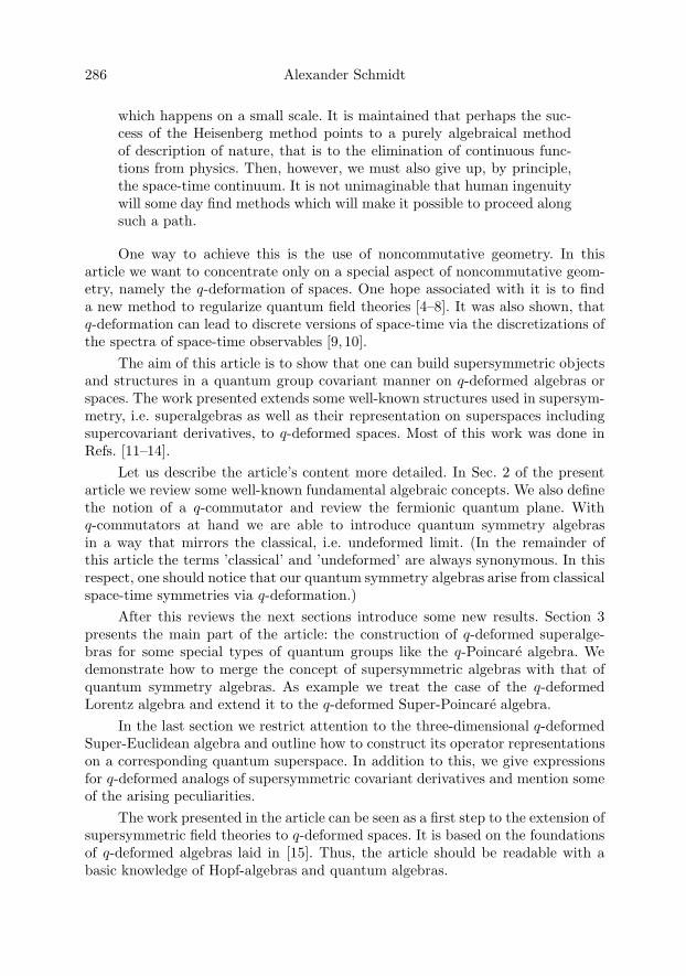
286 Alexander Schmidt
which happens on a small scale. It is maintained that perhaps the suc-cess of the Heisenberg method points to a purely algebraical methodof description of nature, that is to the elimination of continuous func-tions from physics. Then, however, we must also give up, by principle,the space-time continuum. It is not unimaginable that human ingenuitywill some day find methods which will make it possible to proceed alongsuch a path.
One way to achieve this is the use of noncommutative geometry. In thisarticle we want to concentrate only on a special aspect of noncommutative geom-etry, namely the q-deformation of spaces. One hope associated with it is to finda new method to regularize quantum field theories [4–8]. It was also shown, thatq-deformation can lead to discrete versions of space-time via the discretizations ofthe spectra of space-time observables [9, 10].
The aim of this article is to show that one can build supersymmetric objectsand structures in a quantum group covariant manner on q-deformed algebras orspaces. The work presented extends some well-known structures used in supersym-metry, i.e. superalgebras as well as their representation on superspaces includingsupercovariant derivatives, to q-deformed spaces. Most of this work was done inRefs. [11–14].
Let us describe the article’s content more detailed. In Sec. 2 of the presentarticle we review some well-known fundamental algebraic concepts. We also definethe notion of a q-commutator and review the fermionic quantum plane. Withq-commutators at hand we are able to introduce quantum symmetry algebrasin a way that mirrors the classical, i.e. undeformed limit. (In the remainder ofthis article the terms ’classical’ and ’undeformed’ are always synonymous. In thisrespect, one should notice that our quantum symmetry algebras arise from classicalspace-time symmetries via q-deformation.)
After this reviews the next sections introduce some new results. Section 3presents the main part of the article: the construction of q-deformed superalge-bras for some special types of quantum groups like the q-Poincare algebra. Wedemonstrate how to merge the concept of supersymmetric algebras with that ofquantum symmetry algebras. As example we treat the case of the q-deformedLorentz algebra and extend it to the q-deformed Super-Poincare algebra.
In the last section we restrict attention to the three-dimensional q-deformedSuper-Euclidean algebra and outline how to construct its operator representationson a corresponding quantum superspace. In addition to this, we give expressionsfor q-deformed analogs of supersymmetric covariant derivatives and mention someof the arising peculiarities.
The work presented in the article can be seen as a first step to the extension ofsupersymmetric field theories to q-deformed spaces. It is based on the foundationsof q-deformed algebras laid in [15]. Thus, the article should be readable with abasic knowledge of Hopf-algebras and quantum algebras.

Towards a q-Deformed Supersymmetric Field Theory 287
Let us close with some remarks concerning our notation. Throughout thearticle it is understood that λ ≡ q−q−1 and λ+ ≡ q+q−1. The symbol εαβ denotesthe two-dimensional q-deformed spinor metric with nonzero entries ε12 = −q−1/2
and ε21 = q1/2. It holds εαβ = −εαβ.
Similarly, gAB is the metric of three-dimensional q-deformed Euclidean spacewith gAB = gAB. Its nonzero entries are g+− = −q, g33 = 1, and g−+ = −q−1.
2. Fundamental Algebraic Concepts
In this section we want to review some of the fundamental notions we need forour further explanations. In Sec. 3.1 of Ref. [16] the general idea behind matrixquantum groups was shortly explained [18,19]. The following considerations, how-ever, are based on so-called quantum enveloping algebras as they were proposedby Drinfeld and Jimbo [20–22]. It should be mentioned that both approaches areequivalent in a similar manner as one can deal either with Lie groups or Lie alge-bras.
The most relevant mathematical structure all of our reasonings are basedon is that of a q-deformed symmetry algebra. Let us take as example the sym-metry algebra for three-dimensional q-deformed Euclidean space [23, 25–27]. Forthe sake of completeness and to introduce our conventions we write down all rel-evant formulas, though this is a well-known example. It is given by the quan-tum algebra Uq(su(2)) [23–27], which can be viewed as q-analog of the algebra ofthree-dimensional angular momentum. The algebra is generated by the elementsL+, L−, L3, and τ3 subject to the relations
L±τ3 = q±4τ3L±, L3τ3 = τ3L3,
L−L+ − L+L− = (τ3)−1/2L3,
L±L3 − L3L± = q±1L±(τ3)−1/2. (2.1)
If we recognize that τ3 tends to 1 for q → 1, we regain the common algebra ofthree-dimensional angular momentum in the classical limit.
Finally, let us mention that the quantum algebra Uq(su(2)) is a Hopf algebra.On its generators the corresponding Hopf structure is given by
Δ(L±) = L± ⊗ (τ3)−1/2 + 1⊗ L±,
Δ(L3) = L3 ⊗ (τ3)−1/2 + (τ3)1/2 ⊗ L3,
+ λ(τ3)1/2(q−1L− ⊗ L+ + qL+ ⊗ L−), (2.2)
S(L±) =− L±(τ3)1/2,
S(L3) = (τ3)1/2(q2L+L− − q−2L−L+), (2.3)
ε(LA) = 0, A ∈ {+, 3,−}. (2.4)
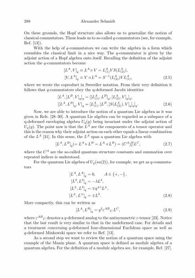
288 Alexander Schmidt
On these grounds, the Hopf structure also allows us to generalize the notion ofclassical commutators. These leads us to so-called q-commutators (see, for example,Ref. [13]).
With the help of q-commutators we can write the algebra in a form whichresembles the classical limit in a nice way. The q-commutator is given by theadjoint action of a Hopf algebra onto itself. Recalling the definition of the adjointaction the q-commutators become
[LA, V ]q ≡ LA V = LA(1)V S(LA
(2)),
[V, LA]q ≡ V ! LA = S−1(LA(2))V LA
(1), (2.5)
where we wrote the coproduct in Sweedler notation. From their very definition itfollows that q-commutators obey the q-deformed Jacobi identities
[LA, [LB, V ]q]q = [[LA(1), L
B]q, [LA(2), V ]q]q,
[[LA, LB]q, V ]q = [LA(1), [L
B, [S(LA(2)), V ]q]q]q. (2.6)
Now, we are able to introduce the notion of a quantum Lie algebra as it wasgiven in Refs. [28–30]. A quantum Lie algebra can be regarded as a subspace of aq-deformed enveloping algebra Uq(g) being invariant under the adjoint action ofUq(g). The point now is that the LA are the components of a tensor operator andthis is the reason why their adjoint action on each other equals a linear combinationof the LA [31]. In this sense, the LA span a quantum Lie algebra with
[LA, LB]q(= LA LB = LA ! LB) = (CA)BCLC , (2.7)
where the CA are the so-called quantum structure constants and summation overrepeated indices is understood.
For the quantum Lie algebra of Uq(su(2)), for example, we get as q-commuta-tors
[LA, LA]q = 0, A ∈ {+,−} ,[L3, L3]q = −λL3,
[L±, L3]q = ∓q±1L±,
[L±, L∓]q = ∓L3. (2.8)
More compactly, this can be written as
[LA, LB]q = q2εABC LC , (2.9)
where εABC denotes a q-deformed analog to the antisymmetric ε-tensor [23]. Notice
that the last result is very similar to that in the undeformed case. For details anda treatment concerning q-deformed four-dimensional Euclidean space as well asq-deformed Minkowski space we refer to Ref. [13].
As a second step we want to review the notion of a quantum space using theexample of the Manin plane. A quantum space is defined as module algebra of aquantum algebra. For the definition of a module algebra see, for example, Ref. [27].

Towards a q-Deformed Supersymmetric Field Theory 289
A physical relevant example for such a module algebra is the quantum plane [32].Its algebra is generated by the elements x1 and x2 subject to the condition
x1x2 = qx2x1. (2.10)
This relation determines what is called the two-dimensional bosonic quantumplane.
In addition to this, there is an antisymmetric variant of the two-dimensionalquantum plane, the so-called fermionic quantum plane. It is generated by thespinor coordinates θ1 and θ2 that satisfy the relations
(θ1)2 = (θ2)2 = 0, θ1θ2 = −q−1θ2θ1, (2.11)
showing the correct classical limit for q → 1. Alternatively, these relations can bewritten with the R-matrix of Uq(su(2)) [15]:
θαθβ = −q−1Rαβγδ θ
γθδ, (2.12)
where
Rαβγδ =
⎛⎜⎜⎝q 0 0 00 λ 1 00 1 0 00 0 0 q
⎞⎟⎟⎠ . (2.13)
For later purposes we introduce conjugate spinor coordinates θα. They againobey the commutation relations in (2.12). There is a braiding between the uncon-jugate and the conjugate quantum plane given by
θ αθβ = −q−1Rαβγδ θ
γ θδ. (2.14)
We can merge the quantum plane and its symmetry algebra resulting in acrossed product. For this, we have to fix relations between the spinor coordinatesand the Uq(su(2))-generators. These are
L+θ1 = θ1L+ − q1/2λ−1/2+ θ2(τ3)−1/2,
L+θ2 = θ2L+, (2.15)
L3θ1 = qθ1L3 − q−1/2λλ−1/2+ θ2L− − qλ−1
+ θ1(τ3)−1/2,
L3θ2 = q−1θ2L3 + q1/2λλ−1/2+ θ1L+ + q−1λ−1
+ θ2(τ3)−1/2, (2.16)
L−θ1 = θ1L−,
L−θ2 = θ2L− + q−1/2λ−1/2+ θ1(τ3)−1/2. (2.17)
We have to take into account the scaling operators Λs which have to be addedas additional generators to the algebra generated by the LA’s. They have triv-ial commutation relations with the LA’s, with spinor coordinates they commuteaccording to
Λsθα = −q1/2θαΛs, Λsθ
α = −q1/2θαΛs. (2.18)

290 Alexander Schmidt
The spinor coordinates carry a Hopf structure, too. Their coproduct reads as
Δ(θ1) = θ1 ⊗ 1 + Λs(τ3)−1/4 ⊗ θ1,
Δ(θ2) = θ2 ⊗ 1 + Λs(τ3)1/4 ⊗ θ2 + q1/2λλ1/2+ Λs(τ3)1/4L+ ⊗ θ1, (2.19)
Δ(θ1) = θ1 ⊗ 1 + Λ−1s (τ3)1/4 ⊗ θ1 + q−1/2λλ
1/2+ Λ−1
s (τ3)1/4L− ⊗ θ2,
Δ(θ2) = θ
2 ⊗ 1 + Λ−1s (τ3)−1/4 ⊗ θ
2. (2.20)
With the help of these coproducts we are in a position to generate the braidingrelations in (2.14), since we have
θαθβ = (θα(1) � θ
β)θα
(2) = θβ
(2)(θα � θ
β
(1)),
θαθβ = (θα(1) � θβ)θα
(2) = θβ(2)(θ
α � θβ(1)). (2.21)
The symbol � and � denote the right- and left adjoint action, respectively. Theleft- and right-adjoint actions are defined as given in (2.5).
3. q-Deformed Superalgebras
In this section we show that it is even possible to extend the symmetry algebras ofq-deformed quantum spaces to q-deformed analogs of superalgebras. If not statedotherwise, in this section we restrict attention to q-deformed Minkowski space andits symmetry algebras, since they are most interesting from a physical point ofview. We build the superalgebra in several steps. At first we extend the q-Lorentzalgebra adding the momentum generators in a consistent way. Doing so we get thewell-known q-Poincare algebra. In a second step we add supergenerators Qα, Qα toget a q-deformed Super-Poincare algebra. The resulting algebra will be an exampleof what we call a q-deformed superalgebra. In the classical limit it turns over intothe well-known Super-Poincare algebra.
Now let us first introduce the subalgebra generated by the components offour-momentum. The momentum algebra of q-deformed Minkowski space isspanned by the momentum components Pμ, μ ∈ {0,+,−, 3} subject to
PμP 0 = P 0Pμ, μ ∈ {0,+,−, 3},P 3P± − q±2P±P 3 = −qλP 0P±,
P−P+ − P+P− = λ(P 3P 3 − P 0P 3). (3.1)
Let us recall that the Pμ, μ ∈ {0,+,−, 3}, behave as a four-vector operatorunder q-deformed Lorentz transformations. This property is a consequence of thecommutation relations between generators of the q-deformed Lorentz algebra andthe corresponding momentum components. They take the form (see also Ref. [13])
[V μν , P ρ]q = −q−1(PA)μνν′ρ′ ηρ′ρP ν′
, (3.2)

Towards a q-Deformed Supersymmetric Field Theory 291
where PA is a q-analog of an antisymmetrizer for q-Minkowski space. The V μν arethe generators of the q-Lorentz algebra written as tensor generators. A detailedtreatment of this algebra can be found in [13].
As a matter of principle the procedure to construct a deformed superalgebrais quite simple. The non-supersymmetric part of the algebra is already known. Itis just the quantum symmetry algebra for the space under consideration combinedwith the corresponding momentum algebra.
What remains is to include spinorial generators in a consistent way. We re-strict ourselves to the case of N = 1 supersymmetry. In complete analogy to theundeformed case we introduce the new generators
Q1, Q2, Q1, Q2. (3.3)
How the spinorial generators commute with the Lorentz algebra generators V μν
is described in Ref. [13]. The result written down in terms of q-commutators is
[V μν , Qα]q = q−1λ−1+ (σμν)β
αQβ ,
[V μν , Qα]q = q−1λ−1+ (σμν)β
αQβ . (3.4)
For the definition of the Pauli matrices see appendix A. Note that the aboverelations are equivalent to the commutation relations in (2.15)-(2.17).
Next we have to fix some sets of relations. These are the relations the super-charges fulfil among themselves, the relations between the supercharges and thegenerators of the symmetry algebra, and finally the relations between momentaand supercharges. This has to be done in a way that the complete algebra gener-ated from V μν , Pμ, Qα, and Qα is consistent with all relations among them, i.e.,every relation remains unchanged after acting with any generator on it.
Since the two types of supercharges Qα and Qα transform as spinors, werequire for them to span quantum planes. In this manner, the supercharges haveto fulfil
QαQα = QαQα = 0, α, α = 1, 2, (3.5)
Q1Q2 = −q−1Q2Q1, Q1Q2 = −q−1Q2Q1. (3.6)
Introducing the q-anticommutator
{θα, θβ}k ≡ θαθβ + kRαβα′β′ θα′
θβ′, (3.7)
the relations in (3.6) become
{Qα, Qβ}q = {Qα, Qβ}q = 0. (3.8)
What remains is to determine the sets of relations QαQβ, PμQα and PμQβ
for μ ∈ {0,+, 3,−} as well as α, β ∈ {1, 2}. For these relations we first makegeneral Ansatze. Then we multiply each relation from the right with a generator,commute the generator to the left, and determine the unknown coefficients fromthe requirement that the relation remains unchanged.

292 Alexander Schmidt
Proceeding this way, we get for the QQ-relations of the q-deformed Super-Poincare algebra
Q1Q1 + Q1Q1 = c q−1P−,
Q1Q2 + q−1Q2Q1 = −q−1λQ1Q2 + c q−1/2λ−1/2+ (P 3 + q−2P 0),
Q2Q1 + q−1Q1Q2 = −c q−3/2λ−1/2+ (P 0 − P 3),
Q2Q2 + Q2Q2 = c q−1P+. (3.9)
For the PQ- and PQ-relations we likewise have
P+Q1 = q−2Q1P+, P+Q2 = Q2P+,
P 0Q1 = q−1Q1P 0, P 0Q2 = q−1Q2P 0,
P 3Q1 = q−1Q1P 3,
P 3Q2 = q−1Q2P 3 + q−3/2λλ1/2+ Q1P+,
P−Q1 = Q1P−,
P−Q2 = q−2Q2P− + q−3/2λλ1/2+ Q1P 3, (3.10)
and
P 0Q1 = qQ1P 0, P 0Q2 = qQ2P 0,
P−Q1 = Q1P−, P−Q2 = q2Q1P−,
P 3Q1 = qQ1P 3 − q3/2λλ1/2+ Q2P−,
P 3Q2 = qQ2P 3,
P+Q1 = q2Q1P+ − q3/2λλ1/2+ Q2P 3,
P+Q2 = Q2P+. (3.11)
Notice that the relations in (3.9) are determined up to a constant c, only. One cancheck that all of the above relations in (3.6), (3.9), (3.10), and (3.11) are compatiblewith the relations concerning the generators V μν of the q-Lorentz algebra.
At last, we list the complete q-deformed supersymmetric Poincare algebra.To this end, we apply our q-commutators introduced earlier since they enable us
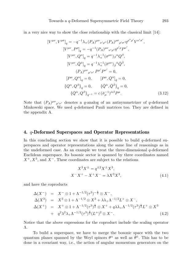
Towards a q-Deformed Supersymmetric Field Theory 293
in a very nice way to show the close relationship with the classical limit [14]:
[V μν , V ρσ]q = −q−1λ+(PA)μνν′ρ′′ (PA)ρσ
ρ′σ′ηρ′′ρ′V ν′σ′
,
[V μν , P ρ]q = −q−1(PA)μνν′ρ′ηρ′ρP ν′
,
[V μν , Qα]q = q−1λ−1+ (σμν)β
αQβ ,
[V μν , Qα]q = q−1λ−1+ (σμν)β
αQβ ,
(PA)μνμ′ν′ Pμ′
P ν′= 0,
[Pμ, Qα]q = 0, [Pμ, Qα]q = 0,
{Qα, Qβ}q = 0, {Qα, Qβ}q = 0,
{Qα, Qβ}q−1 = c (σ−1μ )αβPμ. (3.12)
Note that (PA)μνμ′ν′ denotes a q-analog of an antisymmetrizer of q-deformed
Minkowski space. We used q-deformed Pauli matrices too. They are defined inthe appendix A.
4. q-Deformed Superspaces and Operator Representations
In this concluding section we show that it is possible to build q-deformed su-perspaces and operator representations along the same line of reasonings as inthe undeformed case. As an example we treat the three-dimensional q-deformedEuclidean superspace. Its bosonic sector is spanned by three coordinates namedX+, X3, and X−. These coordinates are subject to the relations
X3X± = q±2X±X3,
X−X+ −X+X− = λX3X3, (4.1)
and have the coproducts
Δ(X−) = X− ⊗ 1 + Λ−1/2(τ3)−12 ⊗X−,
Δ(X3) = X3 ⊗ 1 + Λ−1/2 ⊗X3 + λλ+Λ−1/2L+ ⊗X−,
Δ(X+) = X+ ⊗ 1 + Λ−1/2(τ3)12 ⊗X+ + qλλ+Λ−1/2(τ3)
12L+ ⊗X3
+ q2λ2λ+Λ−1/2(τ3)12 (L+)2 ⊗X−. (4.2)
Notice that the above expressions for the coproduct include the scaling operatorΛ.
To build a superspace, we have to merge the bosonic space with the twoquantum planes spanned by the Weyl spinors θα as well as θα. This has to bedone in a covariant way, i.e., the action of angular momentum generators on the

294 Alexander Schmidt
relations should be zero. Using reasonable Ansatze, we end up with
X+θ1 = qθ1X+ − q1/2λλ1/2+ θ2X3,
X+θ2 = q−1θ2X+,
X3θ1 = θ1X3 − q1/2λλ1/2+ θ2X−,
X3θ2 = θ2X3,
X−θ1 = q−1θ1X−, X−θ2 = qθ2X−. (4.3)
These relations can also be generated from the coproducts in (4.2) as well as fromthe coproducts in (2.20) via
XAθα = (XA(1) � θ
α)XA
(2) = θα
(2)(XA � θ
α
(1)). (4.4)
Applying these identities requires to take account of the fact that Λ acts triviallyon spinor coordinates:
Λ � θα
= θα, (4.5)
as well as Λs on bosonic coordinates
Λs � XA = XA. (4.6)
In Ref. [35] a second construction for the XA was presented, which givesrise to a second set of new, consistent commutation relations between the XA
and the unconjugate spinor coordinates θα. Alternatively, this second set followsfrom conjugating the relations in (4.3) if we take into account the conjugationassignment [15]
θα = −εαβ θβ , θα = εαβθ
β ,
XA = gABXB. (4.7)
Finally, it should be noted that the coproducts in (2.20) and (4.2) respect thecommutation relations in (4.3), i.e. they are consistent with the homomorphismproperty
Δ(XAθα) = Δ(XA)Δ(θα). (4.8)
The coproducts in (4.2) can be extended to q-analogs of supercoproducts. Toachieve this we have to add fermionic parts Δf (XA) to the bosonic coproductsΔ(XA). These fermionic parts are completely determined by making some reason-able claims. First, the new supercoproducts Δs(XA) = Δ(XA) + Δf (XA) shouldbehave under symmetry transformations in the same way as the vector compo-nents XA. In formulas this means Δs(LA � XB) = Δ(LA) � Δs(XB). Further,the supercoproducts should respect the XX-relations in (4.1). Finally, we demandthat the relations in (4.3) are consistent with supercoproducts and the coproductsin (2.20).
To fulfil these requirements we are enforced to introduce a new scaling oper-ator Λk, which helps to adapt the fermionic parts of our supercoproducts to their
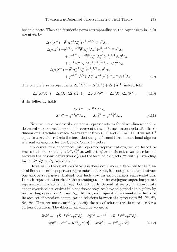
Towards a q-Deformed Supersymmetric Field Theory 295
bosonic parts. Then the fermionic parts corresponding to the coproducts in (4.2)are given by
Δf (X+) =θ2Λ−1s Λ−1
k (τ3)−1/4 ⊗ θ2Λk,
Δf (X3) =q1/2λ−1/2+ θ1Λ−1
s Λ−1k (τ3)−1/4 ⊗ θ2Λk
+ q−1/2λ−1/2+ θ2Λ−1
s Λ−1k (τ3)1/4 ⊗ θ1Λk
+ q−1λθ2Λ−1s Λ−1
k (τ3)1/4L− ⊗ θ2Λk,
Δf (X−) = θ1Λ−1s Λ−1
k (τ3)1/4 ⊗ θ1Λk
+ q−1/2λ1/2+ θ1Λ−1
s Λ−1k (τ3)1/4L− ⊗ θ2Λk. (4.9)
The complete supercoproducts Δs(XA) = Δ(XA) + Δf (XA) indeed fulfil
Δs(XμXν) = Δs(Xμ)Δs(Xν), Δs(Xμθα) = Δs(Xμ)Δs(θα), (4.10)
if the following holds:
ΛkXμ = q−2XμΛk,
Λkθα = q−1θαΛk, Λkθ
α = q−1θαΛk. (4.11)
Now we want to describe operator representations for three-dimensional q-deformed superspace. They should represent the q-deformed superalgebra for three-dimensional Euclidean space. We regain it from (3.1) and (3.8)-(3.11) if we set P 0
equal to zero. This reflects the fact, that the q-deformed three-dimensional algebrais a real subalgebra for the Super-Poincare algebra.
To construct a superspace with operator representations, we are forced torepresent the super charges Qα, Qα as well as to give consistent, covariant relationsbetween the bosonic derivatives ∂A
X and the fermionic objects fα, with fα standingfor θα, θα, ∂α
θ or ∂αθ , respectively.
However, in the quantum space case there occur some differences to the clas-sical limit concerning operator representations. First, it is not possible to constructone unique superspace. Instead, one finds two distinct operator representations.In each representation either the unconjugate or the conjugate supercharges arerepresented in a nontrivial way, but not both. Second, if we try to incorporatesuper covariant derivatives in a consistent way, we have to extend the algebra bynew scaling operators Λn and Λm. At last, each operator representation leads toits own set of covariant commutation relations between the generators ∂A
X , θα, θα,∂α
θ , ∂αθ . Thus, we must carefully specify the set of relations we have to use for a
certain operation. The differential calculus we use is
∂αθ θ
β = −(R−1)αβγδθ
γ∂δθ , ∂α
θ θβ = εαβ − (R−1)αβ
γδ θγ∂δ
θ ,
∂αθ θ
β = εαβ − Rαβγδθ
γ ∂ δθ , ∂α
θ θβ = −Rαβ
γδ θγ ∂ δ
θ . (4.12)

296 Alexander Schmidt
Now we turn to the explicit form of the operator representation with conju-gate supercharges being represented trivially:
Q1 = q−1∂1θΛ−1
m + q3/2θ1∂3XΛm − q3λ+θ
2∂−XΛm,
Q2 = q−1∂2θΛ−1
m − q7/2θ2∂3XΛm + q2λ+θ
1∂+XΛm, (4.13)
Q1 = q−1∂1θΛn, Q2 = q−1∂2
θΛn. (4.14)
Using the q-deformed Pauli matrices (for their explicit form see App. A) we areable to rewrite the above result as
Qα = q−1∂αθ Λ−1
m − q2(σA)αβθ
β∂AXΛm,
Qα = q−1∂αθ Λn. (4.15)
The relations of the q-deformed superalgebra given in Eq. (3.12) are satis-fied by the expressions in (4.15) together with PA = ∂A
XΛnΛm if we assume ascommutation relations
∂+Xθ1 = θ1∂+
X − q−1/2λλ1/2+ θ2∂3
X ,
∂+Xθ2 = q−2θ2∂+
X ,
∂3Xθ1 = q−1θ1∂3
X − q−1/2λλ1/2+ θ2∂−
X ,
∂3Xθ2 = q−1θ2∂3
X ,
∂−Xθ1 = q−2θ1∂−
X , ∂−Xθ2 = θ2∂−
X , (4.16)
and
∂+X θ1 = q2θ1∂+
X − q3/2λλ1/2+ θ2∂3
X ,
∂+X θ2 = θ2∂+
X ,
∂3X θ1 = qθ1∂3
X − q3/2λλ1/2+ θ2∂−
X ,
∂3X θ2 = qθ2∂3
X ,
∂−X θ1 = θ1∂−
X , ∂−X θ2 = q2θ2∂−
X , (4.17)
as well as
∂+X∂1
θ = q−2∂1θ∂
+X , ∂+
X∂2θ = ∂2
θ∂+X ,
∂3X∂1
θ = q−1∂1θ∂
3X ,
∂3X∂2
θ = q−1∂2θ∂
3X + q−3/2λλ+∂
1θ∂
+X ,
∂−X∂1
θ = ∂1θ∂
−X ,
∂−X∂2
θ = q−2∂2θ∂
−X + q−3/2λλ+∂
2θ∂
−X . (4.18)
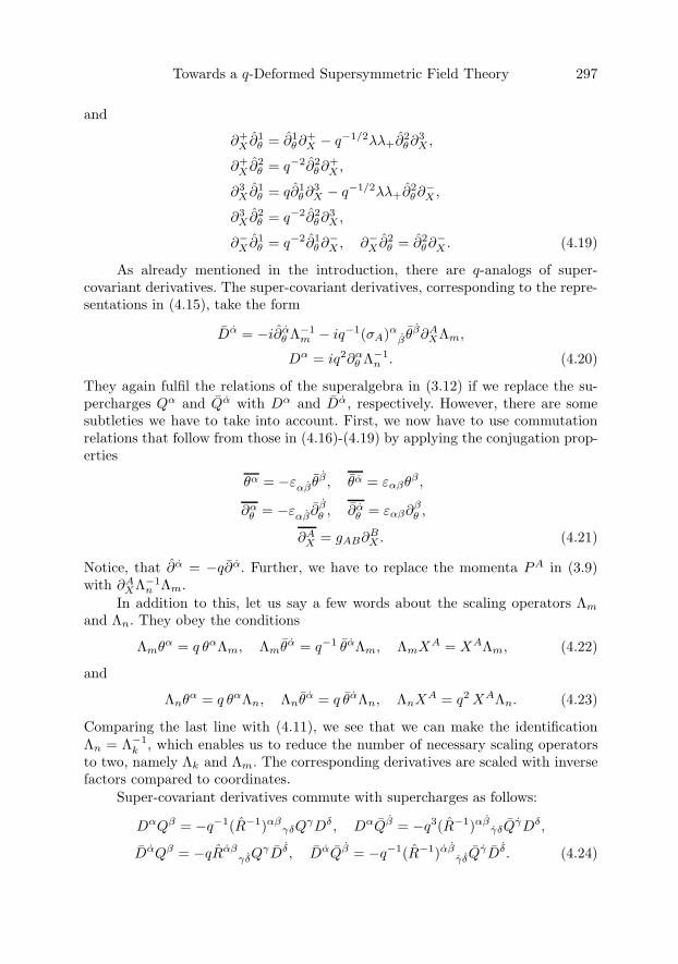
Towards a q-Deformed Supersymmetric Field Theory 297
and
∂+X ∂1
θ = ∂1θ∂
+X − q−1/2λλ+∂
2θ∂
3X ,
∂+X ∂2
θ = q−2∂2θ∂
+X ,
∂3X ∂1
θ = q∂1θ∂
3X − q−1/2λλ+∂
2θ∂
−X ,
∂3X ∂2
θ = q−2∂2θ∂
3X ,
∂−X ∂1
θ = q−2∂1θ∂
−X , ∂−
X ∂2θ = ∂2
θ∂−X . (4.19)
As already mentioned in the introduction, there are q-analogs of super-covariant derivatives. The super-covariant derivatives, corresponding to the repre-sentations in (4.15), take the form
Dα = −i∂αθ Λ−1
m − iq−1(σA)αβ θ
β∂AXΛm,
Dα = iq2∂αθ Λ−1
n . (4.20)
They again fulfil the relations of the superalgebra in (3.12) if we replace the su-percharges Qα and Qα with Dα and Dα, respectively. However, there are somesubtleties we have to take into account. First, we now have to use commutationrelations that follow from those in (4.16)-(4.19) by applying the conjugation prop-erties
θα = −εαβ θβ , θα = εαβθ
β ,
∂αθ = −εαβ∂
βθ , ∂α
θ = εαβ∂βθ ,
∂AX = gAB∂B
X . (4.21)
Notice, that ∂α = −q∂α. Further, we have to replace the momenta PA in (3.9)with ∂A
XΛ−1n Λm.
In addition to this, let us say a few words about the scaling operators Λm
and Λn. They obey the conditions
Λmθα = q θαΛm, Λmθα = q−1 θαΛm, ΛmXA = XAΛm, (4.22)
and
Λnθα = q θαΛn, Λnθ
α = q θαΛn, ΛnXA = q2 XAΛn. (4.23)
Comparing the last line with (4.11), we see that we can make the identificationΛn = Λ−1
k , which enables us to reduce the number of necessary scaling operatorsto two, namely Λk and Λm. The corresponding derivatives are scaled with inversefactors compared to coordinates.
Super-covariant derivatives commute with supercharges as follows:
DαQβ = −q−1(R−1)αβγδQ
γDδ, DαQβ = −q3(R−1)αβγδQ
γDδ,
DαQβ = −qRαβγδQ
γDδ, DαQβ = −q−1(R−1)αβγδQ
γDδ. (4.24)

298 Alexander Schmidt
Moreover, we have to specify the commutation relations between superchargesand fermionic coordinates as well as the commutation relations between covariantderivatives and fermionic coordinates. The former are
Qαθβ = −q−1(R−1)αβγδθ
γQδ,
Qαθβ = εαβΛ−1m − q(R−1)αβ
γδ θγQδ,
Qαθβ = εαβΛn − qRαβγδθ
γQδ,
Qαθβ = −qRαβγδ θ
γQδ, (4.25)
and, likewise, for the latter
Dαθβ = −q−1(R−1)αβγδθ
γDδ,
Dαθβ = iq−1εαβΛ−1n − q−1(R−1)αβ
γδ θγDδ,
Dαθβ = iq−1εαβΛ−1m − q−1Rαβ
γδθγDδ,
Dαθβ = −qRαβγδ θ
γDδ. (4.26)
The relations in (4.16)-(4.19) guarantee that the operator representationsof supercharges fulfil (4.25). However, the operator representations for super-covariant derivatives are only consistent with (4.26) if we use relations that resultfrom (4.16)-(4.19) via the conjugation (4.7). In both cases, the actions of the scal-ing operators are given by (4.22) and (4.23). Finally, it should be mentioned thatwe can write the relations in (4.25) and (4.26) with the help of q-anticommutators[cf. Eq. (3.7)] as
{Qα, Dβ}q = {Qα, Dβ}q−3 = {Dα, Qβ}q = {Qβ , Dα}q = 0. (4.27)
{θα, Qβ}q = {Qα, θβ}q = 0,
{θβ , Qα}q−1 = εαβΛ−1m , {Qα, θβ}q = εαβΛn. (4.28)
{θα, Dβ}q = {Dα, θβ}q = 0,
{θα, Dβ}q = iq−1εαβΛ−1m , {Dβ , θα}q = iq−1εαβΛ−1
n . (4.29)
Appendix A. q-Analogs of Pauli matrices and spin matrices
In this appendix we collect some essential ideas from Ref. [36] concerning q-deformed spinor calculus. We used q-deformed Pauli matrices in Sects. 3 and 4and showed that they enable us to write identities from q-deformed supersymme-try in a way that reveals a remarkable analogy with the classical case.

Towards a q-Deformed Supersymmetric Field Theory 299
Let us recall that the Pauli matrices tell us how to combine two spinors xα, xβ
to form a four-vector Xμ:
Xμ =2∑
α=1, β=1
xα(σμ)αβ xβ , Xμ =
2∑α=1, β=1
xα(σμ)αβxβ . (A.1)
In order to express tensor products of two spinor components by vector componentswe use so-called inverse Pauli matrices:
Xαβ ≡ xαxβ =4∑
μ=1
Xμ(σ−1μ )αβ ,
X αβ ≡ xαxβ =4∑
μ=1
Xμ(σ−1μ )αβ . (A.2)
Explicitly, the q-deformed Pauli matrices are given by
a) (three-dimensional Euclidean space)
(σ+)αβ = q1/2λ1/2+
(0 00 1
), (σ−)αβ = q1/2λ
1/2+
(1 00 0
),
(σ3)αβ =(
0 q1 0
), (A.3)
b) (four-dimensional Euclidean space)
(σ1)αβ =(
1 00 0
), (σ2)αβ =
(0 01 0
),
(σ3)αβ =(
0 10 0
), (σ4)αβ =
(0 00 1
), (A.4)
c) (Minkowski space)
(σ+)αβ =(
0 00 q
), (σ3)αβ = qλ
−1/2+
(0 q1/2
q−1/2 0
),
(σ−)αβ =(
q 00 0
), (σ0)αβ = λ
−1/2+
(0 −q−1/2
q1/2 0
). (A.5)
In Sec. 4 we use the index convention
(σA)αβ = gA′A(σA′
)α′βεα′α. (A.6)
In the case of three-dimensional q-deformed Euclidean space and q-deformedMinkowski space we have
(σμ)γδ = q−1(R−1)αβγδ(σμ)αβ , (A.7)
where (R−1)αβγδ denotes the inverse of the R-matrix for Uq(su(2)) [cf. Eq. (2.13)].
For four-dimensional q-deformed Euclidean space, however, σμ does not differ from

300 Alexander Schmidt
σμ. Finally, the entries of the inverse Pauli matrices are determined by the orthog-onality relations
(σμ)αβ(σ−1ν )αβ = δμ
ν , (σμ)αβ(σ−1ν )αβ = δμ
ν . (A.8)
In analogy to the undeformed case the q-deformed two-dimensional spin ma-trices are defined by
(σμν)αβ ≡ (PA)μν
κλ(σκ)αα εαα′(σλ)α′β′ εβ′β,
(σμν)αβ ≡ (PA)μν
κλ(σκ)αα εαα′(σλ)α′β′ ε
β′β, (A.9)
(σ−1μν )α
β ≡ (PA)κλμν εαα′(σ−1
κ )α′β′εβ′β(σ−1
λ )ββ ,
(σ−1μν )α
β ≡ (PA)κλμν εαα′(σ−1
κ )α′β′εβ′β(σ−1
λ )ββ . (A.10)
Note that PA stands for q-analogs of antisymmetrizers.
Acknowledgement
I am especially grateful to Prof. Eberhard Zeidler. All the results described in thepresent article could only be achieved because he gave me the ability to applymyself, boundlessly, to research activities for the last years. Nowadays, this isabsolutely not self-evident and was only possible because of his special interest inmy work, his confidence and his financial support.
Most of the work presented here was done with my colleague HartmutWachter. I am very grateful to him for his steady support and years of interestingcollaboration. Finally I thank Prof. Dieter Lust for kind hospitality.
References
[1] W. Heisenberg, 1930 Z. Phys. 64 4 & 1938 Ann. Phys. 32 20.
[2] H.S. Snyder, Quantized space-time, Phys. Rev. 71 (1947) 38-41.
[3] A. Einstein Out of My Later Years
[4] H. Grosse, C. Klimcik, and P. Presnajder, Towards finite quantum field theory innon-commutative geometry, 1996 Int. J. Theor. Phys. 35 231 [hep-th/9505175]
[5] S. Majid, On the q-regularisation, 1990 Int. J. Mod. Phys. A 5 4689
[6] R. Oeckl, Braided Quantum Field Theory, 2001 Commun. Math. Phys. 217 451
[7] M. Chaichian, A.P. Demichev, Phys. Lett. B 320 273 (1994) [hep-th/9310001]
[8] C. Blohmann, Free q-deformed relativistic wave equations by representation theory,2003 Eur. Phys. J. C 30 435 [hep-th/0111172]
[9] M. Fichtmuller, A. Lorek, and J. Wess, q-deformed Phase Space and its Lattice Struc-ture, 1996 Z. Phys. C 71 533 [hep-th/9511106]; J. Wess, q-deformed phase space andits lattice structure, 1997 Int. J. Mod. Phys. A 12 4997
[10] B.L. Cerchiai and J. Wess, q-Deformed Minkowski Space based on a q-Lorentz Al-gebra, 1998 Eur. Phys. J. C 5 553 [math.QA/9801104]
[11] D. Mikulovic, A. Schmidt and H. Wachter, Grassmann variables on quantum spaces,Eur. Phys. J. C 45 (2006) 529, [hep-th/0407273].
Towards a q-Deformed Supersymmetric Field Theory 301
[12] A. Schmidt and H. Wachter, Superanalysis on quantum spaces, JHEP 0601 (2006)84, [hep-th/0411180].
[13] A. Schmidt and H. Wachter, q-Deformed quantum Lie algebras, J. Geom. Phys. 56(2006), [mat-ph/0500932].
[14] A. Schmidt, H. Wachter q-Deformed Superalgebras, preprint [hep-th/0705.1683].
[15] J. Wess, q-deformed Heisenberg Algebras, in H. Gausterer, H. Grosse and L.Pittner,Eds., Proceedings of the 38. Internationale Universitatswochen fur Kern- und Teilchenphysik, no. 543 in Lect. Notes in Phys., Springer-Verlag, Schladming (2000), math-phy/9910013.
[16] H. Wachter Towards a q-Deformed Quantum Field Theory, Printed in this volume.
[17] H. Wachter, Analysis on q-deformed quantum spaces, Int. J. Mod. Phys. A 22 (2007)95.
[18] S. L. Woronowicz, Compact matrix pseudogroups , Commun. Math. Phys. 111 (1987)613.
[19] N. Yu. Reshetikhin, L. A. Takhtadzhyan and L. D. Faddeev, Quantization of LieGroups and Lie Algebras, Leningrad Math. J. 1 (1990) 193.
[20] V. G. Drinfeld, Hopf algebras and the quantum Yang-Baxter equation, Sov. Math.Dokl. 32 (1985) 254.
[21] M. Jimbo, A q-analogue of U(g) and the Yang-Baxter equation, Lett. Math. Phys.10 (1985) 63.
[22] V. G. Drinfeld, Quantum groups, in A. M. Gleason, ed., Proceedings of the Interna-tional Congress of Mathematicians, Amer. Math. Soc., 798 (1986).
[23] A. Lorek, W. Weich and J. Wess, Non-commutative Euclidean and Minkowski Struc-tures, Z. Phys. C 76 (1997) 375, [q-alg/9702025].
[24] P. P. Kulish and N. Yu. Reshetikin, Quantum linear problem for the Sine-Gordonequation and higher representations, J. Sov. Math. 23 (1983) 2345.
[25] S. Majid, Foundations of Quantum Group Theory, University Press, Cambridge(1995).
[26] M. Chaichian and A. P. Demichev, Introduction to Quantum Groups, World Scien-tific, Singapore (1996).
[27] A. Klimyk, K. Schmudgen, Quantum Groups and their Representations, Springer-Verlag, 1997.
[28] P. Schupp, P. Watts and B. Zumino, Bicovariant Quantum Algebras and QuantumLie algebras, Commun. Math. Phys. 157 (1993) 305.
[29] S. Majid, Quantum and Braided Lie algebras, J. Geom. Phys. 13 (1994) 307.
[30] A. Sudbery, Quantum differential calculus and lie algebras, Int. J. Mod. Phys. A(1993) 228.
[31] L.C. Biedenharn, M. Tartini, On q-Tensor Operators for Quantum Groups, Lett.Math. Phys. 20 (1990) 271-278.
[32] Yu. I. Manin, Quantum Groups and Non-Commutative Geometry, Centre deRecherche Mathematiques, Montreal (1988).
[33] S. Majid, Free braided differential calculus, braided binomial theorem and thebraided exponential map, 1993 J. Mat. Phys. 34 4843.

302 Alexander Schmidt
[34] S. Majid, Introduction to Braided Geometry and q-Minkowski Space, Preprint, 1994[hep-th/9410241]
[35] C. Bauer and H. Wachter, Operator representations on quantum spaces, 2003 Eur.Phys. J. C 31 261 [math-ph/0201023]
[36] A. Schmidt and H. Wachter, Spinor calculus for q-deformed quantum spaces I,preprint, [hep-th/0705.1640].
Alexander SchmidtArnold-Sommerfeld-CenterTheresienstr. 37D–80333 Munchene-mail: [email protected]
Quantum Field TheoryB. Fauser, J. Tolksdorf and E. Zeidler, Eds., 303–424c© 2009 Birkhauser Verlag Basel/Switzerland
L∞-Algebra Connections and Applicationsto String- and Chern-Simons n-Transport
Hisham Sati, Urs Schreiber and Jim Stasheff
Abstract. We give a generalization of the notion of a Cartan-Ehresmann con-nection from Lie algebras to L∞-algebras and use it to study the obstructiontheory of lifts through higher String-like extensions of Lie algebras. We find(generalized) Chern-Simons and BF-theory functionals this way and describeaspects of their parallel transport and quantization.
It is known that over a D-brane the Kalb-Ramond background field ofthe string restricts to a 2-bundle with connection (a gerbe) which can beseen as the obstruction to lifting the PU(H)-bundle on the D-brane to aU(H)-bundle. We discuss how this phenomenon generalizes from the ordi-nary central extension U(1) → U(H) → PU(H) to higher categorical centralextensions, like the String-extension BU(1) → String(G) → G. Here theobstruction to the lift is a 3-bundle with connection (a 2-gerbe): the Chern-Simons 3-bundle classified by the first Pontrjagin class. For G = Spin(n)this obstructs the existence of a String-structure. We discuss how to describethis obstruction problem in terms of Lie n-algebras and their correspond-ing categorified Cartan-Ehresmann connections. Generalizations even beyondString-extensions are then straightforward. For G = Spin(n) the next step is“Fivebrane structures” whose existence is obstructed by certain generalizedChern-Simons 7-bundles classified by the second Pontrjagin class.
Mathematics Subject Classification (2000). Primary 83E30; Secondary 55P20;81T30; 55R45.
Keywords. Cartan-Ehresman connection, L∞-algebra, Chern-Simons theory,BF-theory, 2-bundles, Eilenberg-MacLane spaces, differential greded algebras,branes, strings.
1. Introduction
The study of extended n-dimensional relativistic objects which arise in string the-ory has shown that these couple to background fields which can naturally bethought of as n-fold categorified generalizations of fiber bundles with connection.
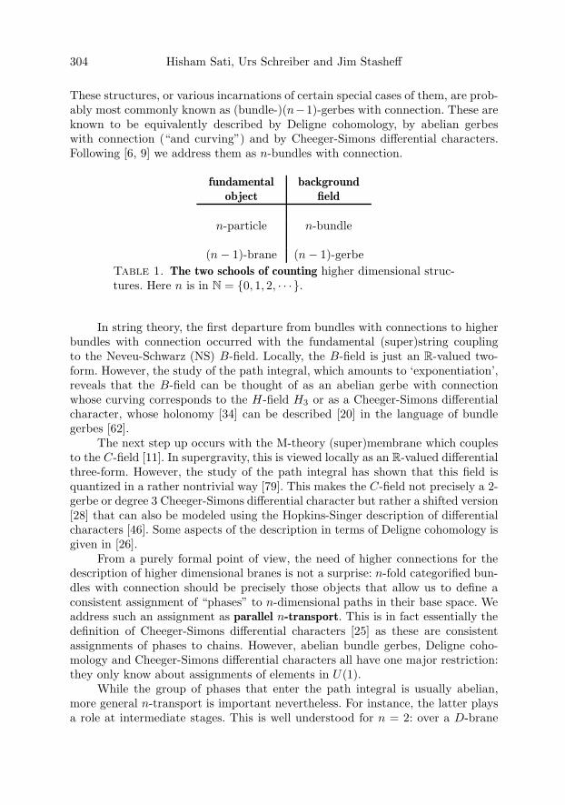
304 Hisham Sati, Urs Schreiber and Jim Stasheff
These structures, or various incarnations of certain special cases of them, are prob-ably most commonly known as (bundle-)(n−1)-gerbes with connection. These areknown to be equivalently described by Deligne cohomology, by abelian gerbeswith connection (“and curving”) and by Cheeger-Simons differential characters.Following [6, 9] we address them as n-bundles with connection.
fundamentalobject
backgroundfield
n-particle n-bundle
(n− 1)-brane (n− 1)-gerbeTable 1. The two schools of counting higher dimensional struc-tures. Here n is in N = {0, 1, 2, · · · }.
In string theory, the first departure from bundles with connections to higherbundles with connection occurred with the fundamental (super)string couplingto the Neveu-Schwarz (NS) B-field. Locally, the B-field is just an R-valued two-form. However, the study of the path integral, which amounts to ‘exponentiation’,reveals that the B-field can be thought of as an abelian gerbe with connectionwhose curving corresponds to the H-field H3 or as a Cheeger-Simons differentialcharacter, whose holonomy [34] can be described [20] in the language of bundlegerbes [62].
The next step up occurs with the M-theory (super)membrane which couplesto the C-field [11]. In supergravity, this is viewed locally as an R-valued differentialthree-form. However, the study of the path integral has shown that this field isquantized in a rather nontrivial way [79]. This makes the C-field not precisely a 2-gerbe or degree 3 Cheeger-Simons differential character but rather a shifted version[28] that can also be modeled using the Hopkins-Singer description of differentialcharacters [46]. Some aspects of the description in terms of Deligne cohomology isgiven in [26].
From a purely formal point of view, the need of higher connections for thedescription of higher dimensional branes is not a surprise: n-fold categorified bun-dles with connection should be precisely those objects that allow us to define aconsistent assignment of “phases” to n-dimensional paths in their base space. Weaddress such an assignment as parallel n-transport. This is in fact essentially thedefinition of Cheeger-Simons differential characters [25] as these are consistentassignments of phases to chains. However, abelian bundle gerbes, Deligne coho-mology and Cheeger-Simons differential characters all have one major restriction:they only know about assignments of elements in U(1).
While the group of phases that enter the path integral is usually abelian,more general n-transport is important nevertheless. For instance, the latter playsa role at intermediate stages. This is well understood for n = 2: over a D-brane
L∞-Algebra Connections and Applications 305
the abelian bundle gerbe corresponding to the NS field has the special propertythat it measures the obstruction to lifting a PU(H)-bundle to a U(H)-bundle, i.e.lifting a bundle with structure group the infinite projective unitary group on aHilbert space H to the corresponding unitary group [15], [16]. Hence, while itselfan abelian 2-structure, it is crucially related to a nonabelian 1-structure.
That this phenomenon deserves special attention becomes clear when wemove up the dimensional ladder: The Green-Schwarz anomaly cancelation [40] inthe heterotic string leads to a 3-structure with the special property that, overthe target space, it measures the obstruction to lifting an E8 × Spin(n)-bundleto a certain nonabelian principal 2-bundle, called a String 2-bundle. Such a 3-structure is also known as a Chern-Simons 2-gerbe [21]. By itself this is abelian,but its structure is constrained by certain nonabelian data. Namely this string 2-bundle with connection, from which the Chern-Simons 3-bundle arises, is itself aninstance of a structure that yields parallel 2-transport. It can be described neitherby abelian bundle gerbes, nor by Cheeger-Simons differential characters, nor byDeligne cohomology.
In anticipation of such situations, previous works have considered nonabeliangerbes and nonabelian bundle gerbes with connection. However, it turns out thatcare is needed in order to find the right setup. For instance, the kinds of non-abelian gerbes with connection studied in [17], [3], although very interesting, arenot sufficiently general to capture String 2-bundles. Moreover, it is not easy tosee how to obtain the parallel 2-transport assignment from these structures. Forthe application to string physics, it would be much more suitable to have a non-abelian generalization of the notion of a Cheeger-Simons differential character, andthus a structure which, by definition, knows how to assign generalized phases ton-dimensional paths.
The obvious generalization that is needed is that of a parallel transport n-functor. Such a notion was described in [9], [72]: a structure defined by the veryfact that it labels n-paths by algebraic objects that allow composition in n differentdirections, such that this composition is compatible with the gluing of n-paths. Onecan show that such transport n-functors encompass abelian and nonabelian gerbeswith connection as special cases [72]. However, these n-functors are more general.For instance, String 2-bundles with connection are given by parallel transport 2-functors. Ironically, the strength of the latter – namely their knowledge aboutgeneral phase assignments to higher dimensional paths – is to some degree also adrawback: for many computations, a description entirely in terms of differentialform data would be more tractable. However, the passage from parallel n-transportto the corresponding differential structure is more or less straightforward: a paralleltransport n-functor is essentially a morphism of Lie n-groupoids. As such, it canbe sent, by a procedure generalizing the passage from Lie groups to Lie algebras,to a morphism of Lie n-algebroids.
The aim of this paper is to describe two topics: First, to set up a formalismfor higher bundles with connections entirely in terms of L∞-algebras, which maybe thought of as a categorification of the theory of Cartan-Ehresmann connections.
306 Hisham Sati, Urs Schreiber and Jim Stasheff
This is supposed to be the differential version of the theory of parallel transportn-functors, but an exhaustive discussion of the differentiation procedure is notgiven here. Instead we discuss a couple of examples and then show how the liftingproblem has a nice description in this language. To do so, we present a family ofL∞-algebras that govern the gauge structure of p-branes, as above, and discuss thelifting problem for them. By doing so, we characterize Chern-Simons 3-forms aslocal connection data on 3-bundles with connection which arise as the obstructionto lifts of ordinary bundles to the corresponding String 2-bundles, governed by theString Lie 2-algebra.
The formalism immediately allows the generalization of this situation tohigher degrees. Indeed we indicate how certain 7-dimensional generalizations ofChern-Simons 3-bundles obstruct the lift of ordinary bundles to certain 6-bundlesgoverned by the Fivebrane Lie 6-algebra. The latter correspond to what we defineas the fivebrane structure, for which the degree seven NS field H7 plays the rolethat the degree three dual NS field H3 plays for the n = 2 case.
The paper is organized in such a way that section 2 serves more or less as aself-contained description of the basic ideas and construction, with the rest of thedocument having all the details and all the proofs.
In this paper we make use of the homotopy algebras usually referred to asL∞-algebras. These algebras also go by other names such as sh-Lie algebras [57].In our context we may also call such algebras Lie ∞-algebras which we think ofas the abstract concept of an ∞-vector space with an antisymmetric bracket ∞-functor on it, which satisfies a Jacobi identity up to coherent equivalence, whereas“L∞-algebra” is concretely a codifferential coalgebra of sorts. In this paper we willnevertheless follow the standard notation of L∞-algebra.
2. The setting and plan
We set up a useful framework for describing higher order bundles with connectionentirely in terms of Lie n-algebras, which can be thought of as arising from acategorification of the concept of an Ehresmann connection on a principal bundle.Then we apply this to the study of Chern-Simons n-bundles with connection asobstructions to lifts of principal G-bundles through higher String-like extensionsof their structure Lie algebra.
2.1. L∞-algebras and their String-like central extensions
A Lie group has all the right properties to locally describe the phase change of acharged particle as it traces out a worldline. A Lie n-group is a higher structurewith precisely all the right properties to describe locally the phase change of acharged (n− 1)-brane as it traces out an n-dimensional worldvolume.
2.1.1. L∞-algebras. Just as ordinary Lie groups have Lie algebras, Lie n-groupshave Lie n-algebras. If the Lie n-algebra is what is called semistrict, these are [5]
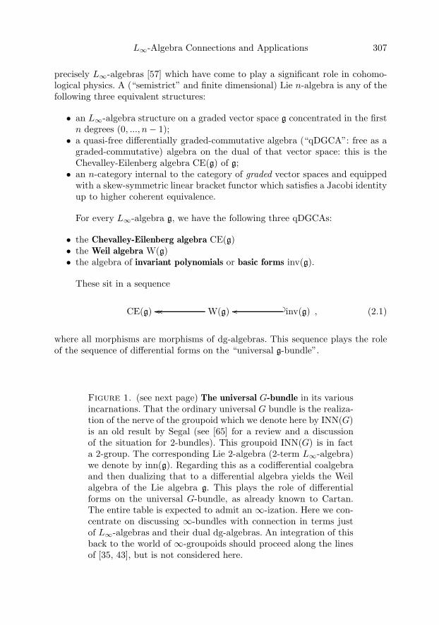
L∞-Algebra Connections and Applications 307
precisely L∞-algebras [57] which have come to play a significant role in cohomo-logical physics. A (“semistrict” and finite dimensional) Lie n-algebra is any of thefollowing three equivalent structures:
• an L∞-algebra structure on a graded vector space g concentrated in the firstn degrees (0, ..., n− 1);
• a quasi-free differentially graded-commutative algebra (“qDGCA”: free as agraded-commutative) algebra on the dual of that vector space: this is theChevalley-Eilenberg algebra CE(g) of g;
• an n-category internal to the category of graded vector spaces and equippedwith a skew-symmetric linear bracket functor which satisfies a Jacobi identityup to higher coherent equivalence.
For every L∞-algebra g, we have the following three qDGCAs:
• the Chevalley-Eilenberg algebra CE(g)• the Weil algebra W(g)• the algebra of invariant polynomials or basic forms inv(g).
These sit in a sequence
CE(g) W(g)���� inv(g)� ��� , (2.1)
where all morphisms are morphisms of dg-algebras. This sequence plays the roleof the sequence of differential forms on the “universal g-bundle”.
Figure 1. (see next page) The universal G-bundle in its variousincarnations. That the ordinary universal G bundle is the realiza-tion of the nerve of the groupoid which we denote here by INN(G)is an old result by Segal (see [65] for a review and a discussionof the situation for 2-bundles). This groupoid INN(G) is in facta 2-group. The corresponding Lie 2-algebra (2-term L∞-algebra)we denote by inn(g). Regarding this as a codifferential coalgebraand then dualizing that to a differential algebra yields the Weilalgebra of the Lie algebra g. This plays the role of differentialforms on the universal G-bundle, as already known to Cartan.The entire table is expected to admit an ∞-ization. Here we con-centrate on discussing ∞-bundles with connection in terms justof L∞-algebras and their dual dg-algebras. An integration of thisback to the world of ∞-groupoids should proceed along the linesof [35, 43], but is not considered here.
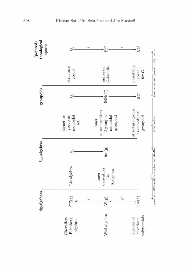
308 Hisham Sati, Urs Schreiber and Jim Stasheff
dg-a
lgeb
ras
L∞
-alg
ebra
sgro
upoid
s(p
oin
ted)
topolo
gic
alsp
aces
Che
valle
y-E
ilenb
erg
alge
bra
CE
(g)
Lie
alge
bra
g� � ��
stru
ctur
egr
oup
asm
onoi
dal
set
G� � ��
stru
ctur
egr
oup
G� � i ��
Wei
lal
gebr
aW
(g)
i∗����
inne
rde
riva
tion
Lie
2-al
gebr
a
inn(
g)
inne
rau
tom
orph
ism
2-gr
oup
asm
onoi
dal
grou
poid
INN
(G)
�� ��
univ
ersa
lG
-bun
dle
EG p �� ��
alge
bra
ofin
vari
ant
poly
nom
ials
inv(
g)
��
p∗
��
stru
ctur
egr
oup
ason
e-ob
ject
grou
poid
BG
clas
sify
ing
spac
efo
rG
BG
�(·)
∗re
gard
as
codiff
ere
nti
alcoalg
ebra
and
dualize
���
Lie
diff
ere
nti
ate
���
|·|ta
ke
nerv
es
and
geom
etr
ically
realize��

L∞-Algebra Connections and Applications 309
2.1.2. L∞-algebras from cocycles: String-like extensions. A simple but importantsource of examples for higher Lie n-algebras comes from the abelian Lie algebrau(1) which may be shifted into higher categorical degrees. We write bn−1u(1) forthe Lie n-algebra which is entirely trivial except in its nth degree, where it lookslike u(1). Just as u(1) corresponds to the Lie group U(1) , so bn−1u(1) correspondsto the iterated classifying space Bn−1U(1), realizable as the topological groupgiven by the Eilenberg-MacLane space K(Z, n). Thus an important source forinteresting Lie n-algebras comes from extensions
0 → bn−1u(1) → g → g → 0 (2.2)
of an ordinary Lie algebra g by such a shifted abelian Lie n-algebra bn−1u(1). Wefind that, for each (n + 1)-cocycle μ in the Lie algebra cohomology of g, we doobtain such a central extension, which we describe by
0 → bn−1u(1) → gμ → g → 0 . (2.3)
Since, for the case when μ = 〈·, [·, ·]〉 is the canonical 3-cocycle on a semisimpleLie algebra g, this gμ is known ([7] and [43]) to be the Lie 2-algebra of the String2-group, we call these central extensions String-like central extensions. (We alsorefer to these as Lie n-algebras “of Baez-Crans type” [5].) Moreover, wheneverthe cocycle μ is related by transgression to an invariant polynomial P on the Liealgebra, we find that gμ fits into a short homotopy exact sequence of Lie (n + 1)-algebras
0 → gμ → csP (μ) → chP (μ) → 0 . (2.4)
Here csP (g) is a Lie (n + 1)-algebra governed by the Chern-Simons term corre-sponding to the transgression element interpolating between μ and P . In a similarfashion chP (g) knows about the characteristic (Chern) class associated with P .
In summary, from elements of the cohomology of CE(g) together with relatedelements in W(g) we obtain the String-like extensions of Lie algebras to Lie 2n-algebras and the associated Chern- and Chern-Simons Lie (2n− 1)-algebras:
Lie algebra cocycle μ Baez-Crans Lie n-algebra gμ
invariant polynomial P Chern Lie n-algebra chP (g)transgression element cs Chern-Simons Lie n-algebra csP (g)
2.1.3. L∞-algebra differential forms. For g an ordinary Lie algebra and Y somemanifold, one finds that dg-algebra morphisms CE(g) → Ω•(Y ) from the Chevally-Eilenberg algebra of g to the DGCA of differential forms on Y are in bijection withg-valued 1-forms A ∈ Ω1(Y, g) whose ordinary curvature 2-form
FA = dA + [A ∧A] (2.5)
vanishes. Without the flatness, the correspondence is with algebra morphisms notrespecting the differentials. But dg-algebra morphisms A : W(g) → Ω•(Y ) are
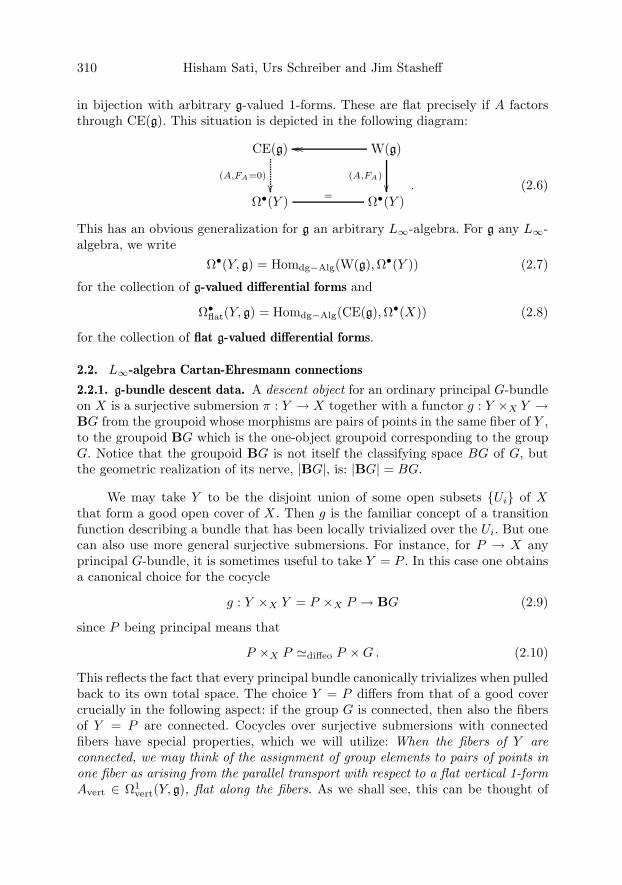
310 Hisham Sati, Urs Schreiber and Jim Stasheff
in bijection with arbitrary g-valued 1-forms. These are flat precisely if A factorsthrough CE(g). This situation is depicted in the following diagram:
CE(g)
(A,FA=0)
��
W(g)����
(A,FA)
��ٕ(Y ) = ٕ(Y )
. (2.6)
This has an obvious generalization for g an arbitrary L∞-algebra. For g any L∞-algebra, we write
Ω•(Y, g) = Homdg−Alg(W(g),Ω•(Y )) (2.7)
for the collection of g-valued differential forms and
Ω•flat(Y, g) = Homdg−Alg(CE(g),Ω•(X)) (2.8)
for the collection of flat g-valued differential forms.
2.2. L∞-algebra Cartan-Ehresmann connections
2.2.1. g-bundle descent data. A descent object for an ordinary principal G-bundleon X is a surjective submersion π : Y → X together with a functor g : Y ×X Y →BG from the groupoid whose morphisms are pairs of points in the same fiber of Y ,to the groupoid BG which is the one-object groupoid corresponding to the groupG. Notice that the groupoid BG is not itself the classifying space BG of G, butthe geometric realization of its nerve, |BG|, is: |BG| = BG.
We may take Y to be the disjoint union of some open subsets {Ui} of Xthat form a good open cover of X . Then g is the familiar concept of a transitionfunction describing a bundle that has been locally trivialized over the Ui. But onecan also use more general surjective submersions. For instance, for P → X anyprincipal G-bundle, it is sometimes useful to take Y = P . In this case one obtainsa canonical choice for the cocycle
g : Y ×X Y = P ×X P → BG (2.9)
since P being principal means that
P ×X P �diffeo P ×G . (2.10)
This reflects the fact that every principal bundle canonically trivializes when pulledback to its own total space. The choice Y = P differs from that of a good covercrucially in the following aspect: if the group G is connected, then also the fibersof Y = P are connected. Cocycles over surjective submersions with connectedfibers have special properties, which we will utilize: When the fibers of Y areconnected, we may think of the assignment of group elements to pairs of points inone fiber as arising from the parallel transport with respect to a flat vertical 1-formAvert ∈ Ω1
vert(Y, g), flat along the fibers. As we shall see, this can be thought of
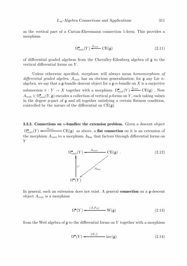
L∞-Algebra Connections and Applications 311
as the vertical part of a Cartan-Ehresmann connection 1-form. This provides amorphism
Ω•vert(Y ) CE(g)
Avert�� (2.11)
of differential graded algebras from the Chevalley-Eilenberg algebra of g to thevertical differential forms on Y .
Unless otherwise specified, morphism will always mean homomorphism ofdifferential graded algebra. Avert has an obvious generalization: for g any Lie n-algebra, we say that a g-bundle descent object for a g-n-bundle on X is a surjective
submersion π : Y → X together with a morphism Ω•vert(Y ) CE(g)
Avert�� . NowAvert ∈ Ω•
vert(Y, g) encodes a collection of vertical p-forms on Y , each taking valuesin the degree p-part of g and all together satisfying a certain flatness condition,controlled by the nature of the differential on CE(g).
2.2.2. Connections on n-bundles: the extension problem. Given a descent object
Ω•vert(Y ) CE(g)
Avert�� as above, a flat connection on it is an extension ofthe morphism Avert to a morphism Aflat that factors through differential forms onY
Ω•vert(Y ) CE(g)
Avert��
Aflat
��ٕ(Y )
i∗
����. (2.12)
In general, such an extension does not exist. A general connection on a g-descentobject Avert is a morphism
ٕ(Y ) W(g)(A,FA)�� (2.13)
from the Weil algebra of g to the differential forms on Y together with a morphism
ٕ(Y ) inv(g){Ki}�� (2.14)

312 Hisham Sati, Urs Schreiber and Jim Stasheff
from the invariant polynomials on g, as in 2.1.1, to the differential forms on X ,such that the following two squares commute:
Ω•vert(Y ) CE(g)
Avert��
Ω•(Y )
i∗
����
W (g)
����
(A,FA)��
ٕ(X)��
π∗
��
inv(g)��
��
{Ki}��
. (2.15)
Whenever we have such two commuting squares, we say
• Avert ∈ Ω•vert(Y, g) is a g-bundle descent object (playing the role of a transi-
tion function);• A ∈ Ω•(Y, g) is a (Cartan-Ehresmann) connection with values in the L∞-
algebra g on the total space of the surjective submersion;• FA ∈ Ω•+1(Y, g) are the corresponding curvature forms;• and the set {Ki ∈ Ω•(X)} are the corresponding characteristic forms, whose
classes {[Ki]} in de Rham cohomology
ٕ(X) inv(g){Ki}��
H•deRham(X) H•(inv(g))
{[Ki]}��
(2.16)
are the corresponding characteristic classes of the given descent object Avert.
Hence we realize the curvature of a g-connection as the obstruction to ex-tending a g-descent object to a flat g-connection.
2.3. Higher string and Chern-Simons n-transport: the lifting problem
Given a g-descent object
CE(g)
Avert�������
����
Ω•vert(Y )
, (2.17)

L∞-Algebra Connections and Applications 313
Ω•vert(Y ) CE(g)
Avert�� descentdata
firstCartan-Ehresmann
condition
Ω•(Y )
i∗
����
W (g)
����
(A,FA)�� connectiondata
secondCartan-Ehresmann
condition
ٕ(X)��
π∗
��
inv(g)��
��
{Ki}�� characteristicforms
H•dR(X) H•(inv(g)){[Ki]}
�� Chern-Weilhomomorphism
Figure 2. A g-connection descent object and its interpretation.For g-any L∞-algebra and X a smooth space, a g-connection onX is an equivalence class of pairs (Y, (A,FA)) consisting of a sur-jective submersion π : Y → X and dg-algebra morphisms formingthe above commuting diagram. The equivalence relation is con-cordance of such diagrams. The situation for ordinary Cartan-Ehresmann (1-)connections is described in 6.2.1.
and given an extension of g by a String-like L∞-algebra
CE(bn−1u(1)) CE(gμ)i���� CE(g)� ��� , (2.18)
we ask if it is possible to lift the descent object through this extension, i.e. to finda dotted arrow in
CE(bn−1u(1)) CE(gμ)����
��
CE(g)� ���
Avert��������
Ω•vert(Y )
. (2.19)
In general this is not possible. We seek a straightforward way to compute theobstruction to the existence of the lift. The strategy is to form the weak (homotopy)
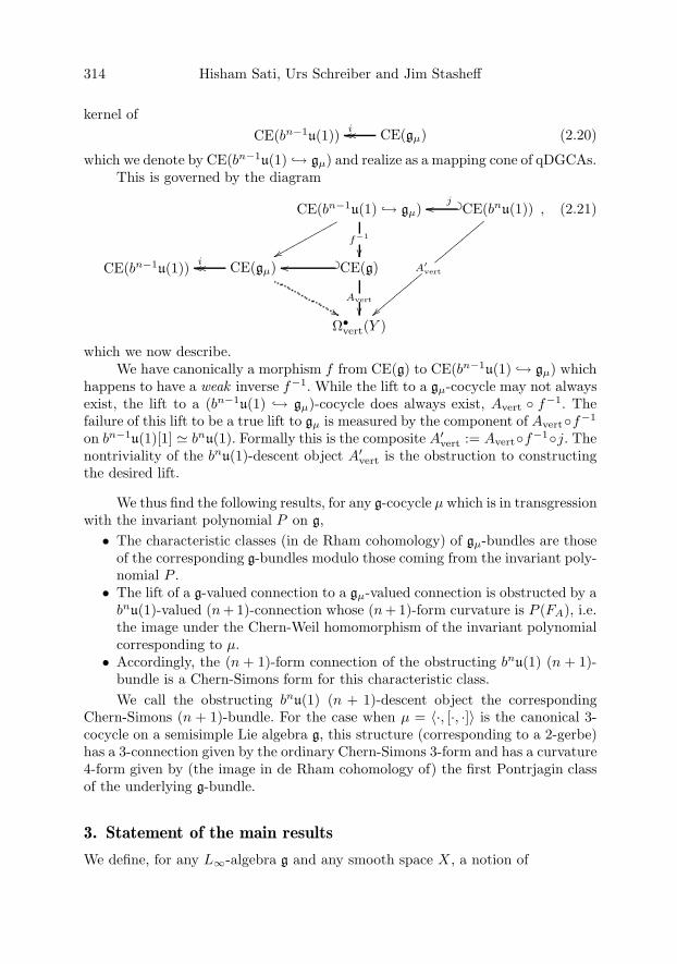
314 Hisham Sati, Urs Schreiber and Jim Stasheff
kernel ofCE(bn−1u(1)) CE(gμ)i���� (2.20)
which we denote by CE(bn−1u(1) ↪→ gμ) and realize as a mapping cone of qDGCAs.This is governed by the diagram
CE(bn−1u(1) ↪→ gμ)
������
����
f−1
��
CE(bnu(1))� �j��
A′vert
���������
���������CE(bn−1u(1)) CE(gμ)i����
��
CE(g)� ���
Avert
��ٕ
vert(Y )
, (2.21)
which we now describe.We have canonically a morphism f from CE(g) to CE(bn−1u(1) ↪→ gμ) which
happens to have a weak inverse f−1. While the lift to a gμ-cocycle may not alwaysexist, the lift to a (bn−1u(1) ↪→ gμ)-cocycle does always exist, Avert ◦ f−1. Thefailure of this lift to be a true lift to gμ is measured by the component of Avert◦f−1
on bn−1u(1)[1] � bnu(1). Formally this is the composite A′vert := Avert◦f−1◦j. The
nontriviality of the bnu(1)-descent object A′vert is the obstruction to constructing
the desired lift.
We thus find the following results, for any g-cocycle μ which is in transgressionwith the invariant polynomial P on g,• The characteristic classes (in de Rham cohomology) of gμ-bundles are those
of the corresponding g-bundles modulo those coming from the invariant poly-nomial P .
• The lift of a g-valued connection to a gμ-valued connection is obstructed by abnu(1)-valued (n+ 1)-connection whose (n+ 1)-form curvature is P (FA), i.e.the image under the Chern-Weil homomorphism of the invariant polynomialcorresponding to μ.
• Accordingly, the (n + 1)-form connection of the obstructing bnu(1) (n + 1)-bundle is a Chern-Simons form for this characteristic class.We call the obstructing bnu(1) (n + 1)-descent object the corresponding
Chern-Simons (n + 1)-bundle. For the case when μ = 〈·, [·, ·]〉 is the canonical 3-cocycle on a semisimple Lie algebra g, this structure (corresponding to a 2-gerbe)has a 3-connection given by the ordinary Chern-Simons 3-form and has a curvature4-form given by (the image in de Rham cohomology of) the first Pontrjagin classof the underlying g-bundle.
3. Statement of the main results
We define, for any L∞-algebra g and any smooth space X , a notion of

L∞-Algebra Connections and Applications 315
• g-descent objects over X ;and an extension of these to• g-connection descent objects over X .
These descent objects are to be thought of as the data obtained from locallytrivializing an n-bundle (with connection) whose structure n-group has the Lie n-algebra g. Being differential versions of n-functorial descent data of such n-bundles,they consist of morphisms of quasi free differential graded-commutative algebras(qDGCAs).
We define for each L∞-algebra g a dg-algebra inv(g) of invariant polynomialson g. We show that every g-connection descent object gives rise to a collection ofde Rham classes on X : its characteristic classes. These are images of the elementsof inv(g). Two descent objects are taken to be equivalent if they are concordant ina natural sense.
Our first main result is
Theorem 3.1 (Characteristic classes). Characteristic classes are indeed character-istic of g-descent objects (but do not necessarily fully characterize them) in thefollowing sense:• Concordant g-connection descent objects have the same characteristic classes.• If the g-connection descent objects differ just by a gauge transformation, they
even have the same characteristic forms.
This is our proposition 6.9 and corollary 6.10.Remark. We expect that this result can be strengthened. Currently our charac-teristic classes are just in de Rham cohomology. One would expect that these areimages of classes in integral cohomology. While we do not attempt here to discussintegral characteristic classes in general, we discuss some aspects of this for thecase of abelian Lie n-algebras g = bn−1u(1) in 6.1.1 by relating g-descent objectsto Deligne cohomology.
The reader should also note that in our main examples to be discussed insection 7 we start with an L∞-connection which happens to be an ordinary Cartan-Ehresmann connection on an ordinary bundle and is hence known to have integralclasses. It follows from our results then that also the corresponding Chern-Simons3-connections in particular have an integral class.
We define String-like extensions gμ of L∞-algebras coming from any L∞-algebra cocycle μ: a closed element in the Chevalley-Eilenberg dg-algebra CE(g)corresponding to g: μ ∈ CE(g). These generalize the String Lie 2-algebra whichgoverns the dynamics of (heterotic) superstrings.
Our second main results is
Theorem 3.2 (String-like extensions and their properties). For every degree (n+1)-cocycle μ on an L∞-algebra g we obtain the String-like extension gμ which sits inan exact sequence
0 → bn−1u(1) → gμ → g → 0 .
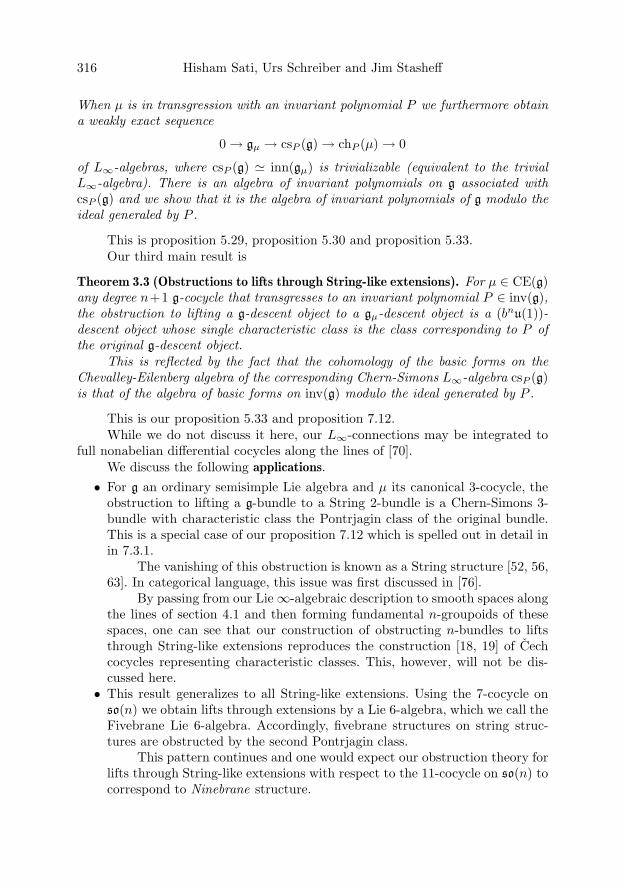
316 Hisham Sati, Urs Schreiber and Jim Stasheff
When μ is in transgression with an invariant polynomial P we furthermore obtaina weakly exact sequence
0 → gμ → csP (g) → chP (μ) → 0
of L∞-algebras, where csP (g) � inn(gμ) is trivializable (equivalent to the trivialL∞-algebra). There is an algebra of invariant polynomials on g associated withcsP (g) and we show that it is the algebra of invariant polynomials of g modulo theideal generaled by P .
This is proposition 5.29, proposition 5.30 and proposition 5.33.Our third main result is
Theorem 3.3 (Obstructions to lifts through String-like extensions). For μ ∈ CE(g)any degree n+1 g-cocycle that transgresses to an invariant polynomial P ∈ inv(g),the obstruction to lifting a g-descent object to a gμ-descent object is a (bnu(1))-descent object whose single characteristic class is the class corresponding to P ofthe original g-descent object.
This is reflected by the fact that the cohomology of the basic forms on theChevalley-Eilenberg algebra of the corresponding Chern-Simons L∞-algebra csP (g)is that of the algebra of basic forms on inv(g) modulo the ideal generated by P .
This is our proposition 5.33 and proposition 7.12.While we do not discuss it here, our L∞-connections may be integrated to
full nonabelian differential cocycles along the lines of [70].We discuss the following applications.
• For g an ordinary semisimple Lie algebra and μ its canonical 3-cocycle, theobstruction to lifting a g-bundle to a String 2-bundle is a Chern-Simons 3-bundle with characteristic class the Pontrjagin class of the original bundle.This is a special case of our proposition 7.12 which is spelled out in detail inin 7.3.1.
The vanishing of this obstruction is known as a String structure [52, 56,63]. In categorical language, this issue was first discussed in [76].
By passing from our Lie ∞-algebraic description to smooth spaces alongthe lines of section 4.1 and then forming fundamental n-groupoids of thesespaces, one can see that our construction of obstructing n-bundles to liftsthrough String-like extensions reproduces the construction [18, 19] of Cechcocycles representing characteristic classes. This, however, will not be dis-cussed here.
• This result generalizes to all String-like extensions. Using the 7-cocycle onso(n) we obtain lifts through extensions by a Lie 6-algebra, which we call theFivebrane Lie 6-algebra. Accordingly, fivebrane structures on string struc-tures are obstructed by the second Pontrjagin class.
This pattern continues and one would expect our obstruction theory forlifts through String-like extensions with respect to the 11-cocycle on so(n) tocorrespond to Ninebrane structure.
L∞-Algebra Connections and Applications 317
The issue of p-brane structures for higher p was discussed before in [60].In contrast to the discussion there, we here see p-brane structures only forp = 4n+1, corresponding to the list of invariant polynomials and cocycles forso(n). While our entire obstruction theory applies to all cocycles on all Lie∞-algebras, it is only for those on so(n) and maybe e8 for which the physicalinterpretation in the sense of p-brane structures is understood.
• We discuss how the action functional of the topological field theory known asBF-theory arises from an invariant polynomial on a strict Lie 2-algebra, in ageneralization of the integrated Pontrjagin 4-form of the topological term inYang-Mills theory. See proposition 5.26 and the example in 5.6.1.
This is similar to but different from the Lie 2-algebraic interpretationof BF theory indicated in [38, 39], where the “cosmological” bilinear in theconnection 2-form is not considered and a constraint on the admissible strictLie 2-algebras is imposed.
• We indicate in 8.1 the notion of parallel transport induced by a g-connection,relate it to the n-functorial parallel transport of [9, 72, 73, 74] and point outhow this leads to σ-model actions in terms of dg-algebra morphisms. Seesection 8.
• We indicate in 8.3.1 how by forming configuration spaces by sending DGCAsto smooth spaces and then using the internal hom of smooth space, we obtainfor every g-connection descent object configuration spaces of maps equippedwith an action functional induced by the transgressed g-connection. We showthat the algebra of differential forms on these configuration spaces naturallysupports the structure of the corresponding BRST-BV complex, with theiterated ghost-of-ghost structure inherited from the higher degree symmetriesinduced by g.
This construction is similar in spirit to the one given in [1], reviewed in[66], but also, at least superficially, a bit different.
• We indicate also in 8.3.1 how this construction of configuration spaces inducesthe notion of transgression of n-bundles on X to (n−k)-bundles on spaces ofmaps from k-dimensional spaces into X . An analogous integrated descriptionof transgression in terms of inner homs is in [73]. We show in 8.3.1 in partic-ular that this transgression process relates the concept of String-structuresin terms of 4-classes down on X with the corresponding 3-classes on LX , asdiscussed for instance in [56]. Our construction immediately generalizes tofivebrane and higher classes.
All of our discussion here pertains to principal L∞-connections. One canalso discuss associated g-connections induced by (∞-)representations of g (for in-stance as in [58]) and then study the collections of “sections” or “modules” of suchassociated g-connections.
The extended quantum field theory of a (n − 1)-brane charged under an n-connection (“a charged n-particle”, definition 8.5) should (see for instance [32,33, 76, 45]) assign to each d-dimensional part Σ of the brane’s parameter space

318 Hisham Sati, Urs Schreiber and Jim Stasheff
(“worldvolume”) the collection (an (n−d−1)-category, really) of sections/modulesof the transgression of the n-bundle to the configuration space of maps from Σ.
For instance, the space of sections of a Chern-Simons 3-connection trans-gressed to maps from the circle should yield the representation category of theKac-Moody extension of the corresponding loop group.
Our last proposition 8.6 points in this direction. But a more detailed discus-sion will not be given here.
4. Differential graded-commutative algebra
Differential N-graded commutative algebras (DGCAs) play a prominent role in ourdiscussion. One way to understand what is special about DGCAs is to realize thatevery DGCA can be regarded, essentially, as the algebra of differential forms onsome generalized smooth space.
We explain what this means precisely in section 4.1. The underlying phenom-enon is essentially the familiar governing principle of Sullivan models in rationalhomotopy theory [44, 77], but instead of working with simplicial spaces, we hereconsider presheaf categories. This will not become relevant, though, until the dis-cussion of configuration spaces, parallel transport and action functionals in section8.
4.1. Differential forms on smooth spaces
We can think of every differential graded commutative algebra essentially as beingthe algebra of differential forms on some space, possibly a generalized space.
Definition 4.1. Let S be the category whose objects are the open subsets of R∪R2∪R3 ∪ · · · and whose morphisms are smooth maps between these. We write
S∞ := SetSop(4.1)
for the category of set-valued presheaves on S.
So an object X in S∞ is an assignment of sets U �→ X(U) to each opensubset U , together with an assignment
( Uφ �� V ) �→ ( X(U) ��
φ∗X
X(V ) ) (4.2)
of maps of sets to maps of smooth subsets which respects composition. A morphism
f : X → Y (4.3)
of smooth spaces is an assignment U �→ ( X(U)fU �� Y (U) ) of maps of sets to
open subsets, such that for all smooth maps of subsets Uφ �� V we have that
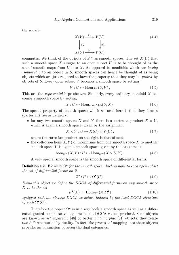
L∞-Algebra Connections and Applications 319
the square
X(V )fV ��
φ∗X
��
Y (V )
φ∗Y
��X(U)
fU �� Y (U)
(4.4)
commutes. We think of the objects of S∞ as smooth spaces. The set X(U) thatsuch a smooth space X assigns to an open subset U is to be thought of as theset of smooth maps from U into X . As opposed to manifolds which are locallyisomorphic to an object in S, smooth spaces can hence be thought of as beingobjects which are just required to have the property that they may be probed byobjects of S. Every open subset V becomes a smooth space by setting
V : U �→ HomS∞(U, V ) . (4.5)
This are the representable presheaves. Similarly, every ordinary manifold X be-comes a smooth space by setting
X : U �→ Hommanifolds(U,X) . (4.6)
The special property of smooth spaces which we need here is that they form a(cartesian) closed category:• for any two smooth spaces X and Y there is a cartesian product X × Y ,
which is again a smooth space, given by the assignment
X × Y : U �→ X(U)× Y (U) ; (4.7)
where the cartesian product on the right is that of sets;• the collection hom(X,Y ) of morphisms from one smooth space X to another
smooth space Y is again a smooth space, given by the assignment
homS∞(X,Y ) : U �→ HomS∞(X × U, Y ) . (4.8)
A very special smooth space is the smooth space of differential forms.
Definition 4.2. We write Ω• for the smooth space which assigns to each open subsetthe set of differential forms on it
Ω• : U �→ Ω•(U) . (4.9)
Using this object we define the DGCA of differential forms on any smooth spaceX to be the set
Ω•(X) := HomS∞(X,Ω•) (4.10)equipped with the obvious DGCA structure induced by the local DGCA structureof each Ω•(U).
Therefore the object Ω• is in a way both a smooth space as well as a differ-ential graded commutative algebra: it is a DGCA-valued presheaf. Such objectsare known as schizophrenic [48] or better ambimorphic [81] objects: they relatetwo different worlds by duality. In fact, the process of mapping into these objectsprovides an adjunction between the dual categories:
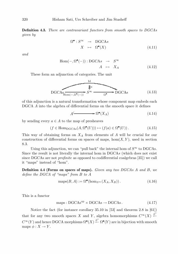
320 Hisham Sati, Urs Schreiber and Jim Stasheff
Definition 4.3. There are contravariant functors from smooth spaces to DGCAsgiven by
Ω• : S∞ → DGCAs
X �→ Ω•(X) (4.11)
and
Hom(−,Ω•(−)) : DGCAs → S∞
A �→ XA (4.12)
These form an adjunction of categories. The unit
DGCAs
Id
��
Hom(−,Ω•(−))�� S∞
ٕ�� DGCAs
u
(4.13)
of this adjunction is a natural transformation whose component map embeds eachDGCA A into the algebra of differential forms on the smooth space it defines
A� � �� ٕ(XA) (4.14)
by sending every a ∈ A to the map of presheaves
(f ∈ HomDGCAs(A,Ω•(U))) �→ (f(a) ∈ Ω•(U)) . (4.15)
This way of obtaining forms on XA from elements of A will be crucial for ourconstruction of differential forms on spaces of maps, hom(X,Y ), used in section8.3.
Using this adjunction, we can “pull back” the internal hom of S∞ to DGCAs.Since the result is not literally the internal hom in DGCAs (which does not existsince DGCAs are not profinite as opposed to codifferential coalgebras [35]) we callit “maps” instead of “hom”.
Definition 4.4 (Forms on spaces of maps). Given any two DGCAs A and B, wedefine the DGCA of “maps” from B to A
maps(B,A) := Ω•(homS∞(XA, XB)) . (4.16)
This is a functor
maps : DGCAsop ×DGCAs → DGCAs . (4.17)
Notice the fact (for instance corollary 35.10 in [53] and theorem 2.8 in [61])
that for any two smooth spaces X and Y , algebra homomorphisms C∞(X)φ∗←
C∞(Y ) and hence DGCA morphisms Ω•(X)φ∗← Ω•(Y ) are in bijection with smooth
maps φ : X → Y .
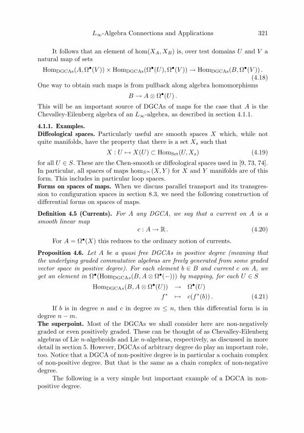
L∞-Algebra Connections and Applications 321
It follows that an element of hom(XA, XB) is, over test domains U and V anatural map of sets
HomDGCAs(A,Ω•(V ))×HomDGCAs(Ω•(U),Ω•(V )) → HomDGCAs(B,Ω•(V )) .(4.18)
One way to obtain such maps is from pullback along algebra homomorphisms
B → A⊗ Ω•(U) .
This will be an important source of DGCAs of maps for the case that A is theChevalley-Eilenberg algebra of an L∞-algebra, as described in section 4.1.1.
4.1.1. Examples.Diffeological spaces. Particularly useful are smooth spaces X which, while notquite manifolds, have the property that there is a set Xs such that
X : U �→ X(U) ⊂ HomSet(U,Xs) (4.19)
for all U ∈ S. These are the Chen-smooth or diffeological spaces used in [9, 73, 74].In particular, all spaces of maps homS∞(X,Y ) for X and Y manifolds are of thisform. This includes in particular loop spaces.Forms on spaces of maps. When we discuss parallel transport and its transgres-sion to configuration spaces in section 8.3, we need the following construction ofdifferential forms on spaces of maps.
Definition 4.5 (Currents). For A any DGCA, we say that a current on A is asmooth linear map
c : A→ R . (4.20)
For A = Ω•(X) this reduces to the ordinary notion of currents.
Proposition 4.6. Let A be a quasi free DGCAs in positive degree (meaning thatthe underlying graded commutative algebras are freely generated from some gradedvector space in positive degree). For each element b ∈ B and current c on A, weget an element in Ω•(HomDGCAs(B,A⊗ Ω•(−))) by mapping, for each U ∈ S
HomDGCAs(B,A⊗ Ω•(U)) → Ω•(U)f∗ �→ c(f∗(b)) . (4.21)
If b is in degree n and c in degree m ≤ n, then this differential form is indegree n−m.The superpoint. Most of the DGCAs we shall consider here are non-negativelygraded or even positively graded. These can be thought of as Chevalley-Eilenbergalgebras of Lie n-algebroids and Lie n-algebras, respectively, as discussed in moredetail in section 5. However, DGCAs of arbitrary degree do play an important role,too. Notice that a DGCA of non-positive degree is in particular a cochain complexof non-positive degree. But that is the same as a chain complex of non-negativedegree.
The following is a very simple but important example of a DGCA in non-positive degree.

322 Hisham Sati, Urs Schreiber and Jim Stasheff
Definition 4.7 (Superpoint). The “algebra of functions on the superpoint” is theDGCA
C(pt) := (R⊕ R[−1], dpt) (4.22)
where the product on R ⊕ R[−1] is the tensor product over R, and where the dif-ferential dpt : R[−1] → R is the canonical isomorphism.
The smooth space associated to this algebra according to definition 4.3 isjust the ordinary point, because for any test domain U the set
HomDGCAs(C(pt),Ω•(U)) (4.23)
contains only the morphism which sends 1 ∈ R to the constant unit function onU , and which sends R[−1] to 0. However, as is well known from the theory ofsupermanifolds, the algebra C(pt) is important in that morphisms from any otherDGCA A into it compute the (shifted) tangent space corresponding to A. Fromour point of view here this manifests itself in particular by the fact that for X anymanifold, we have a canonical injection
Ω•(TX) ↪→ Ω•(maps(C∞(X), C(pt))) (4.24)
of the differential forms on the tangent bundle of X into the differential forms onthe smooth space of algebra homomorphisms of C∞(X) to C(pt):
for every test domain U an element in HomDGCAs(C∞(X), C(pt ⊗ Ω•(U)))comes from a pair consisting of a smooth map f : U → X and a vector fieldv ∈ Γ(TX). Together this constitutes a smooth map f : U → TX and hencefor every form ω ∈ Ω•(TX) we obtain a form on maps(C∞(X), C(pt)) by theassignment
((f, v) ∈ HomDGCAs(C∞(X), C(pt⊗ Ω•(U)))) �→ (f∗ω ∈ Ω•(U)) (4.25)
over each test domain U .In section 5.1.1 we discuss how in the analogous fashion we obtain the Weil
algebra W(g) of any L∞-algebra g from its Chevalley-Eilenberg algebra CE(g) bymapping that to C(pt). This says that the Weil algebra is like the space of functionson the shifted tangent bundle of the “space” that the Chevalley-Eilenberg algebrais the space of functions on. See also figure 3.
4.2. Homotopies and inner derivations
When we forget the algebra structure of DGCAs, they are simply cochain com-plexes. As such they naturally live in a 2-category Ch• whose objects are cochaincomplexes (V •, dV ), whose morphisms
(V •, dV ) (W •, dW )f∗
�� (4.26)
are degree preserving linear maps V • W •f∗�� that do respect the differentials,
[d, f∗] := dV ◦ f∗ − f∗ ◦ dW = 0 , (4.27)

L∞-Algebra Connections and Applications 323
and whose 2-morphisms
(V •, dV ) (W •, dW )
f∗
��
g∗
��ρ
(4.28)
are cochain homotopies, namely linear degree -1 maps ρ : W • → V • with theproperty that
g∗ = f∗ + [d, ρ] = f∗ + dV ◦ ρ + ρ ◦ dW . (4.29)Later in section 5.2 we will also look at morphisms that do preserve the algebrastructure, and homotopies of these. Notice that we can compose a 2-morphismfrom left and right with 1-morphisms, to obtain another 2-morphism
(U•, dU ) (V •, dV )h∗�� (W •, dW )
f∗
��
g∗
��(X•, dX)
j∗��ρ
(4.30)whose component map now is
h∗ ◦ ρ ◦ j∗ : X• j∗ �� W • ρ �� V • h∗�� U• . (4.31)
This will be important for the interpretation of the diagrams we discuss, of thetype (4.40) and (4.46) below.
Of special importance are linear endomorphisms V • V •ρ�� of DGCAswhich are algebra derivations. Among them, the inner derivations in turn play aspecial role:
Definition 4.8 (Inner derivations). On any DGCA (V •, dV ), a degree 0 endomor-phism
(V •, dV ) (V •, dV )L�� (4.32)
is called an inner derivation if• it is an algebra derivation of degree 0;• it is connected to the 0-derivation, i.e. there is a 2-morphims
(V •, dV ) (V •, dV )
0
��
L=[dV ,ρ]
��ρ
, (4.33)
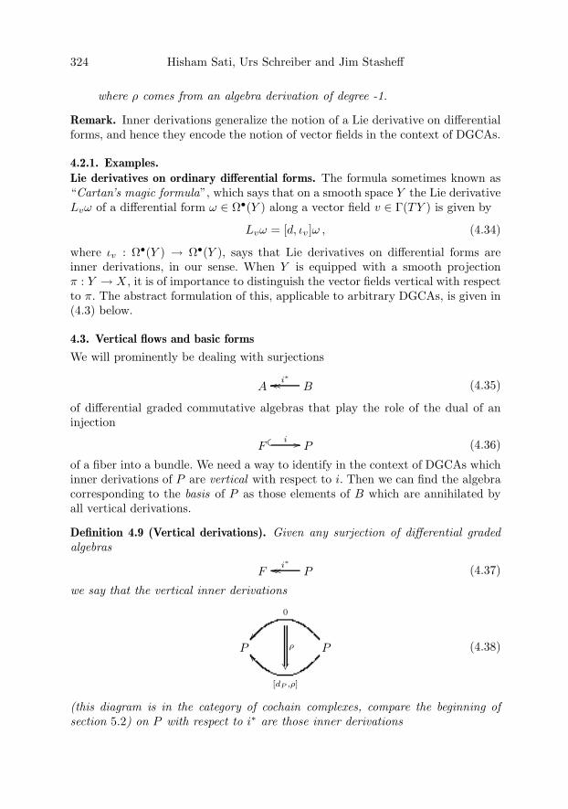
324 Hisham Sati, Urs Schreiber and Jim Stasheff
where ρ comes from an algebra derivation of degree -1.
Remark. Inner derivations generalize the notion of a Lie derivative on differentialforms, and hence they encode the notion of vector fields in the context of DGCAs.
4.2.1. Examples.
Lie derivatives on ordinary differential forms. The formula sometimes known as“Cartan’s magic formula”, which says that on a smooth space Y the Lie derivativeLvω of a differential form ω ∈ Ω•(Y ) along a vector field v ∈ Γ(TY ) is given by
Lvω = [d, ιv]ω , (4.34)
where ιv : Ω•(Y ) → Ω•(Y ), says that Lie derivatives on differential forms areinner derivations, in our sense. When Y is equipped with a smooth projectionπ : Y → X , it is of importance to distinguish the vector fields vertical with respectto π. The abstract formulation of this, applicable to arbitrary DGCAs, is given in(4.3) below.
4.3. Vertical flows and basic forms
We will prominently be dealing with surjections
A Bi∗���� (4.35)
of differential graded commutative algebras that play the role of the dual of aninjection
F� � i �� P (4.36)
of a fiber into a bundle. We need a way to identify in the context of DGCAs whichinner derivations of P are vertical with respect to i. Then we can find the algebracorresponding to the basis of P as those elements of B which are annihilated byall vertical derivations.
Definition 4.9 (Vertical derivations). Given any surjection of differential gradedalgebras
F Pi∗���� (4.37)
we say that the vertical inner derivations
P P
0
��
[dP ,ρ]
��ρ
(4.38)
(this diagram is in the category of cochain complexes, compare the beginning ofsection 5.2) on P with respect to i∗ are those inner derivations

L∞-Algebra Connections and Applications 325
• for which there exists an inner derivation of F
F F
0
��
[dP ,ρ′]
�� ρ′
(4.39)
such that
F F
[d,ρ′]
��
0
P
����
P
����
[d,ρ]
��
0
ρ′
ρ
; (4.40)
• and where ρ′ is a contraction, ρ′ = ιx, i.e. a derivation which sends inde-composables to degree 0.
Definition 4.10 (Basic elements). Given any surjection of differential graded alge-bras
F Pi∗���� (4.41)
we say that the algebra
Pbasic =⋂
ρ vertical
ker(ρ) ∩ ker(ρ ◦ dp) (4.42)
of basic elements of P (with respect to the surjection i∗) is the subalgebra of P ofall those elements a ∈ P which are annihilated by all i∗-vertical derivations ρ, inthat
ρ(a) = 0 (4.43)ρ(dP a) = 0 . (4.44)
We have a canonical inclusion
P Pbasic� �
p∗�� . (4.45)
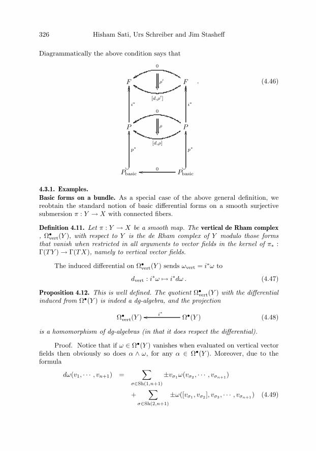
326 Hisham Sati, Urs Schreiber and Jim Stasheff
Diagrammatically the above condition says that
F F
[d,ρ′]
��
0
��
P
i∗
����
P
i∗
����
[d,ρ]
��
0
��
Pbasic
��
p∗
��
Pbasic
��
p∗
��
0��
ρ′
ρ
. (4.46)
4.3.1. Examples.
Basic forms on a bundle. As a special case of the above general definition, wereobtain the standard notion of basic differential forms on a smooth surjectivesubmersion π : Y → X with connected fibers.
Definition 4.11. Let π : Y → X be a smooth map. The vertical de Rham complex, Ω•
vert(Y ), with respect to Y is the de Rham complex of Y modulo those formsthat vanish when restricted in all arguments to vector fields in the kernel of π∗ :Γ(TY ) → Γ(TX), namely to vertical vector fields.
The induced differential on Ω•vert(Y ) sends ωvert = i∗ω to
dvert : i∗ω �→ i∗dω . (4.47)
Proposition 4.12. This is well defined. The quotient Ω•vert(Y ) with the differential
induced from Ω•(Y ) is indeed a dg-algebra, and the projection
Ω•vert(Y ) Ω•(Y )i∗�� (4.48)
is a homomorphism of dg-algebras (in that it does respect the differential).
Proof. Notice that if ω ∈ Ω•(Y ) vanishes when evaluated on vertical vectorfields then obviously so does α ∧ ω, for any α ∈ Ω•(Y ). Moreover, due to theformula
dω(v1, · · · , vn+1) =∑
σ∈Sh(1,n+1)
±vσ1ω(vσ2 , · · · , vσn+1)
+∑
σ∈Sh(2,n+1)
±ω([vσ1 , vσ2 ], vσ3 , · · · , vσn+1) (4.49)

L∞-Algebra Connections and Applications 327
and the fact that for v, w vertical so is [v, w] and hence dω is also vertical. Thisgives that vertical differential forms on Y form a dg-subalgebra of the algebra ofall forms on Y . Therefore if i∗ω = i∗ω′ then
di∗ω′ = i∗dω′ = i∗d(ω + (ω′ − ω)) = i∗dω + 0 = di∗ω . (4.50)
Hence the differential is well defined and i∗ is then, by construction, a morphismof dg-algebras.
�
Recall the following standard definition of basic differential forms.
Definition 4.13 (Basic forms). Given a surjective submersion π : Y → X, thebasic forms on Y are those with the property that they and their differentials areannihilated by all vertical vector fields
ω ∈ Ω•(Y )basic ⇔ ∀v ∈ ker(π) : ιvω = ιvdω = 0 . (4.51)
It is a standard result that
Proposition 4.14. If π : Y → X is locally trivial and has connected fibers, then thebasic forms are precisely those coming from pullback along π
Ω•(Y )basic � Ω•(X) . (4.52)
Remark. The reader should compare this situation with the definition of invariantpolynomials in section 5.3.
The next proposition asserts that these statements about ordinary basic dif-ferential forms are indeed a special case of the general definition of basic elementswith respect to a surjection of DGCAs, definition 4.10.
Proposition 4.15. Given a surjective submersion π : Y → X with connected fibers,then
• the inner derivations of Ω•(Y ) which are vertical with respect to
Ω•vert(Y ) Ω•(Y )i∗���� according to the general definition 4.9, come precisely
from contractions ιv with vertical vector fields v ∈ ker(π∗) ⊂ Γ(TY );• the basic differential forms on Y according to definition 4.13 coincide with
the basic elements of Ω•(Y ) relative to the above surjection
Ω•vert(Y ) Ω•(Y )i∗���� (4.53)
according to the general definition 4.10.
Proof. We first show that if Ω•(Y ) Ω•(Y )ρ�� is a vertical algebra deriva-
tion, then ρ has to annihilate all forms in the image of π∗. Let α ∈ Ω•(Y ) be any
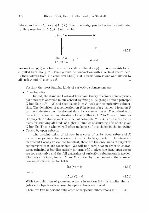
328 Hisham Sati, Urs Schreiber and Jim Stasheff
1-form and ω = π∗β for β ∈ Ω1(X). Then the wedge product α ∧ ω is annihilatedby the projection to Ω•
vert(Y ) and we find
ρ(ω) ∧ α 0���
ρ(ω) ∧ α+ρ(α) ∧ ω
�
i∗
��
α ∧ ω�
i∗
��
�ρ��
. (4.54)
We see that ρ(ω) ∧ α has to vanish for all α. Therefore ρ(ω) has to vanish for allω pulled back along π∗. Hence ρ must be contraction with a vertical vector field.It then follows from the condition (4.40) that a basic form is one annihilated byall such ρ and all such ρ ◦ d. �
Possibly the most familiar kinds of surjective submersions are• Fiber bundles.
Indeed, the standard Cartan-Ehresmann theory of connections of princi-pal bundles is obtained in our context by fixing a Lie group G and a principalG-bundle p : P → X and then using Y = P itself as the surjective submer-sion. The definition of a connection on P in terms of a g-valued 1-form on Pcan be understood as the descent data for a connection on P obtained withrespect to canonical trivialization of the pullback of P to Y = P . Using forthe surjective submersion Y a principal G-bundle P → X is also most conve-nient for studying all kinds of higher n-bundles obstructing lifts of the givenG-bundle. This is why we will often make use of this choice in the following.
• Covers by open subsets.The disjoint union of all sets in a cover of X by open subsets of X
forms a surjective submersion π : Y → X . In large parts of the literatureon descent (locally trivialized bundles), these are the only kinds of surjectivesubmersions that are considered. We will find here, that in order to charac-terize principal n-bundles entirely in terms of L∞-algebraic data, open coversare too restrictive and the full generality of surjective submersions is needed.The reason is that, for π : Y → X a cover by open subsets, there are nonontrivial vertical vector fields
ker(π) = 0, (4.55)
henceΩ•
vert(Y ) = 0 . (4.56)
With the definition of g-descent objects in section 6.1 this implies that allg-descent objects over a cover by open subsets are trivial.There are two important subclasses of surjective submersions π : Y → X :

L∞-Algebra Connections and Applications 329
• those for which Y is (smoothly) contractible;• those for which the fibers of Y are connected.
We say Y is (smoothly) contractible if the identity map Id : Y → Y is(smoothly) homotopic to a map Y → Y which is constant on each connectedcomponent. Hence Y is a disjoint union of spaces that are each (smoothly) con-tractible to a point. In this case the Poincare lemma says that the dg-algebraΩ•(Y ) of differential forms on Y is contractible; each closed form is exact:
Ω•(Y ) Ω•(Y )
0
[d,τ ]
��τ
. (4.57)
Here τ is the familiar homotopy operator that appears in the proof of the Poincarelemma. In practice, we often make use of the best of both worlds: surjective submer-sions that are (smoothly) contractible to a discrete set but still have a sufficientlyrich collection of vertical vector fields. The way to obtain these is by refinement:starting with any surjective submersion π : Y → X which has good vertical vec-tor fields but might not be contractible, we can cover Y itself with open balls,whose disjoint union, Y ′, then forms a surjective submersion Y ′ → Y over Y . Thecomposite π′
Y ′
�
����
���
�� Y
��
X
(4.58)
is then a contractible surjective submersion of X . We will see that all our descentobjects can be pulled back along refinements of surjective submersions this way, sothat it is possible, without restriction of generality, to always work on contractiblesurjective submersions. Notice that for these the structure of
ٕvert(Y ) ٕ(Y )���� ٕ(X)� ��� (4.59)
is rather similar to that of
CE(g) W(g)���� inv(g)� ��� , (4.60)
since W(g) is also contractible, according to proposition 5.7.Vertical derivations on universal g-bundles. The other important example of ver-tical flows, those on DGCAs modeling universal g-bundle for g an L∞-algebra, isdiscussed at the beginning of section 5.3.
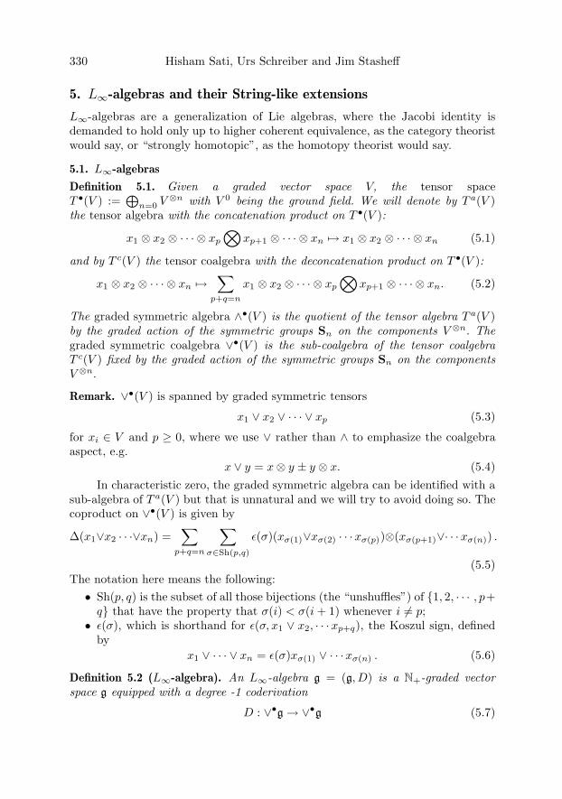
330 Hisham Sati, Urs Schreiber and Jim Stasheff
5. L∞-algebras and their String-like extensions
L∞-algebras are a generalization of Lie algebras, where the Jacobi identity isdemanded to hold only up to higher coherent equivalence, as the category theoristwould say, or “strongly homotopic”, as the homotopy theorist would say.
5.1. L∞-algebras
Definition 5.1. Given a graded vector space V, the tensor spaceT •(V ) :=
⊕n=0 V
⊗n with V 0 being the ground field. We will denote by T a(V )the tensor algebra with the concatenation product on T •(V ):
x1 ⊗ x2 ⊗ · · · ⊗ xp
⊗xp+1 ⊗ · · · ⊗ xn �→ x1 ⊗ x2 ⊗ · · · ⊗ xn (5.1)
and by T c(V ) the tensor coalgebra with the deconcatenation product on T •(V ):
x1 ⊗ x2 ⊗ · · · ⊗ xn �→∑
p+q=n
x1 ⊗ x2 ⊗ · · · ⊗ xp
⊗xp+1 ⊗ · · · ⊗ xn. (5.2)
The graded symmetric algebra ∧•(V ) is the quotient of the tensor algebra T a(V )by the graded action of the symmetric groups Sn on the components V ⊗n. Thegraded symmetric coalgebra ∨•(V ) is the sub-coalgebra of the tensor coalgebraT c(V ) fixed by the graded action of the symmetric groups Sn on the componentsV ⊗n.
Remark. ∨•(V ) is spanned by graded symmetric tensors
x1 ∨ x2 ∨ · · · ∨ xp (5.3)
for xi ∈ V and p ≥ 0, where we use ∨ rather than ∧ to emphasize the coalgebraaspect, e.g.
x ∨ y = x⊗ y ± y ⊗ x. (5.4)In characteristic zero, the graded symmetric algebra can be identified with a
sub-algebra of T a(V ) but that is unnatural and we will try to avoid doing so. Thecoproduct on ∨•(V ) is given by
Δ(x1∨x2 · · ·∨xn) =∑
p+q=n
∑σ∈Sh(p,q)
ε(σ)(xσ(1)∨xσ(2) · · ·xσ(p))⊗(xσ(p+1)∨· · ·xσ(n)) .
(5.5)The notation here means the following:• Sh(p, q) is the subset of all those bijections (the “unshuffles”) of {1, 2, · · · , p+q} that have the property that σ(i) < σ(i + 1) whenever i �= p;
• ε(σ), which is shorthand for ε(σ, x1 ∨ x2, · · ·xp+q), the Koszul sign, definedby
x1 ∨ · · · ∨ xn = ε(σ)xσ(1) ∨ · · ·xσ(n) . (5.6)
Definition 5.2 (L∞-algebra). An L∞-algebra g = (g, D) is a N+-graded vectorspace g equipped with a degree -1 coderivation
D : ∨•g → ∨•g (5.7)

L∞-Algebra Connections and Applications 331
on the graded co-commutative coalgebra generated by g, such that D2 = 0. Thisinduces a differential
dCE(g) : Sym•(g) → Sym•+1(g) (5.8)
on graded-symmetric multilinear functions on g. When g is finite dimensional thisyields a degree +1 differential
dCE(g) : ∧•g∗ → ∧•g∗ (5.9)
on the graded-commutative algebra generated from g∗. This is the Chevalley-Eilen-berg dg-algebra corresponding to the L∞-algebra g. If g∗ is concentrated in degree1, . . . , n, we also say that g is a Lie n-algebra.
Remark. That the original definition of L∞-algebras in terms of multibracketsyields a codifferential coalgebra as above was shown in [57]. That every such cod-ifferential comes from a collection of multibrackets this way is due to [58].Example. For (g[−1], [·, ·]) an ordinary Lie algebra (meaning that we regard thevector space g to be in degree 1), the corresponding Chevalley-Eilenberg qDGCAis
CE(g) = (∧•g∗, dCE(g)) (5.10)
with
dCE(g) : g∗[·,·]∗ �� g∗ ∧ g∗ . (5.11)
If we let {ta} be a basis of g and {Cabc} the corresponding structure constants of
the Lie bracket [·, ·], and if we denote by {ta} the corresponding basis of g∗, thenwe get
dCE(g)ta = −1
2Ca
bctb ∧ tc . (5.12)
Notice that built in we have a shift of degree for convenience, which makes ordinaryLie 1-algebras be in degree 1 already. In much of the literature a Lie n-algebrawould be based on a vector space concentrated in degrees 0 to n− 1. An ordinaryLie algebra is a Lie 1-algebra. Here the coderivation differential D = [·, ·] is justthe Lie bracket, extended as a coderivation to ∨•g, with g regarded as being indegree 1.
In the rest of the paper we assume, just for simplicity and since it is sufficientfor our applications, all g to be finite-dimensional. Then, by the above, these L∞-algebras are equivalently conceived of in terms of their dual Chevalley-Eilenbergalgebras, CE(g), as indeed every quasi-free differential graded commutative algebra(“qDGCA”, meaning that it is free as a graded commutative algebra) correspondsto an L∞-algebra. We will find it convenient to work entirely in terms of qDGCAs,which we will usually denote as CE(g).
While not very interesting in themselves, truly free differential algebras area useful tool for handling quasi-free differential algebras.
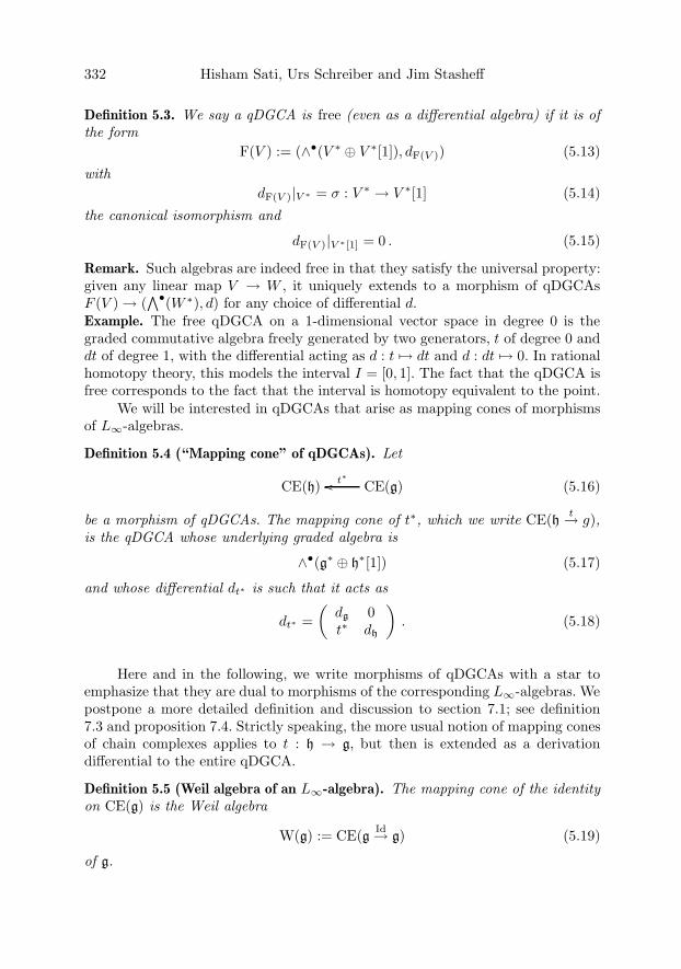
332 Hisham Sati, Urs Schreiber and Jim Stasheff
Definition 5.3. We say a qDGCA is free (even as a differential algebra) if it is ofthe form
F(V ) := (∧•(V ∗ ⊕ V ∗[1]), dF(V )) (5.13)
withdF(V )|V ∗ = σ : V ∗ → V ∗[1] (5.14)
the canonical isomorphism and
dF(V )|V ∗[1] = 0 . (5.15)
Remark. Such algebras are indeed free in that they satisfy the universal property:given any linear map V → W , it uniquely extends to a morphism of qDGCAsF (V ) → (
∧•(W ∗), d) for any choice of differential d.Example. The free qDGCA on a 1-dimensional vector space in degree 0 is thegraded commutative algebra freely generated by two generators, t of degree 0 anddt of degree 1, with the differential acting as d : t �→ dt and d : dt �→ 0. In rationalhomotopy theory, this models the interval I = [0, 1]. The fact that the qDGCA isfree corresponds to the fact that the interval is homotopy equivalent to the point.
We will be interested in qDGCAs that arise as mapping cones of morphismsof L∞-algebras.
Definition 5.4 (“Mapping cone” of qDGCAs). Let
CE(h) CE(g)t∗�� (5.16)
be a morphism of qDGCAs. The mapping cone of t∗, which we write CE(h t→ g),is the qDGCA whose underlying graded algebra is
∧•(g∗ ⊕ h∗[1]) (5.17)
and whose differential dt∗ is such that it acts as
dt∗ =(
dg 0t∗ dh
). (5.18)
Here and in the following, we write morphisms of qDGCAs with a star toemphasize that they are dual to morphisms of the corresponding L∞-algebras. Wepostpone a more detailed definition and discussion to section 7.1; see definition7.3 and proposition 7.4. Strictly speaking, the more usual notion of mapping conesof chain complexes applies to t : h → g, but then is extended as a derivationdifferential to the entire qDGCA.
Definition 5.5 (Weil algebra of an L∞-algebra). The mapping cone of the identityon CE(g) is the Weil algebra
W(g) := CE(g Id→ g) (5.19)
of g.

L∞-Algebra Connections and Applications 333
Proposition 5.6. For g an ordinary Lie algebra this does coincide with the ordinaryWeil algebra of g.
Proof. See the example in section 5.1.1. �
The Weil algebra has two important properties.
Proposition 5.7. The Weil algebra W(g) of any L∞-algebra g
• is isomorphic to a free differential algebra
W(g) � F(g) , (5.20)
and hence is contractible;• has a canonical surjection
CE(g) W(g)i∗���� . (5.21)
Proof. Define a morphism
f : F(g) → W(g) (5.22)
by setting
f : a �→ a (5.23)f : (dF(V )a = σa) �→ (dW(g)a = dCE(g)a + σa) (5.24)
for all a ∈ g∗ and extend as an algebra homomorphism. This clearly respects thedifferentials: for all a ∈ V ∗ we find
a � dF (g) ���
f
��
σa�
f��
a �dW(g)
�� dCE(g)a + σa
and
σa � dF (g) ���
f
��
0�f
��dW(g)a
�dW(g)
�� 0
. (5.25)
One checks that the strict inverse exists and is given by
f−1|g∗ : a �→ a (5.26)
f−1|g∗[1] : σa �→ dF (g)a− dCE(g)a . (5.27)
Here σ : g∗ → g∗[1] is the canonical isomorphism that shifts the degree. The
surjection CE(g) W(g)i∗���� simply projects out all elements in the shifted copyof g:
i∗|∧•g∗ = id (5.28)i∗|g∗[1] = 0 . (5.29)
This is an algebra homomorphism that respects the differential. �
As a corollary we obtain
Corollary 5.8. For g any L∞-algebra, the cohomology of W(g) is trivial.
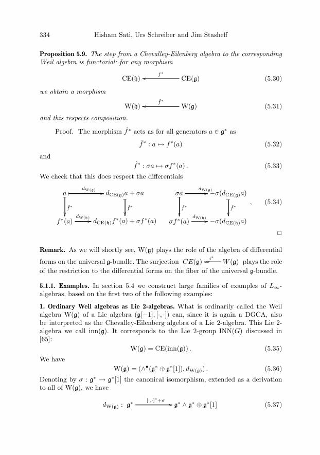
334 Hisham Sati, Urs Schreiber and Jim Stasheff
Proposition 5.9. The step from a Chevalley-Eilenberg algebra to the correspondingWeil algebra is functorial: for any morphism
CE(h) CE(g)f∗
�� (5.30)
we obtain a morphism
W(h) W(g)f∗
�� (5.31)
and this respects composition.
Proof. The morphism f∗ acts as for all generators a ∈ g∗ as
f∗ : a �→ f∗(a) (5.32)
andf∗ : σa �→ σf∗(a) . (5.33)
We check that this does respect the differentials
a�
f∗
��
� dW(g) �� dCE(g)a + σa�
f∗
��f∗(a)
dW(h) �� dCE(h)f∗(a) + σf∗(a)
σa�
f∗
��
� dW(g)�� −σ(dCE(g)a)�
f∗
��σf∗(a)
dW(h) �� −σ(dCE(h)a)
, (5.34)
�
Remark. As we will shortly see, W(g) plays the role of the algebra of differential
forms on the universal g-bundle. The surjection CE(g) W (g)i∗���� plays the roleof the restriction to the differential forms on the fiber of the universal g-bundle.
5.1.1. Examples. In section 5.4 we construct large families of examples of L∞-algebras, based on the first two of the following examples:
1. Ordinary Weil algebras as Lie 2-algebras. What is ordinarily called the Weilalgebra W(g) of a Lie algebra (g[−1], [·, ·]) can, since it is again a DGCA, alsobe interpreted as the Chevalley-Eilenberg algebra of a Lie 2-algebra. This Lie 2-algebra we call inn(g). It corresponds to the Lie 2-group INN(G) discussed in[65]:
W(g) = CE(inn(g)) . (5.35)
We haveW(g) = (∧•(g∗ ⊕ g∗[1]), dW(g)) . (5.36)
Denoting by σ : g∗ → g∗[1] the canonical isomorphism, extended as a derivationto all of W(g), we have
dW(g) : g∗[·,·]∗+σ �� g∗ ∧ g∗ ⊕ g∗[1] (5.37)
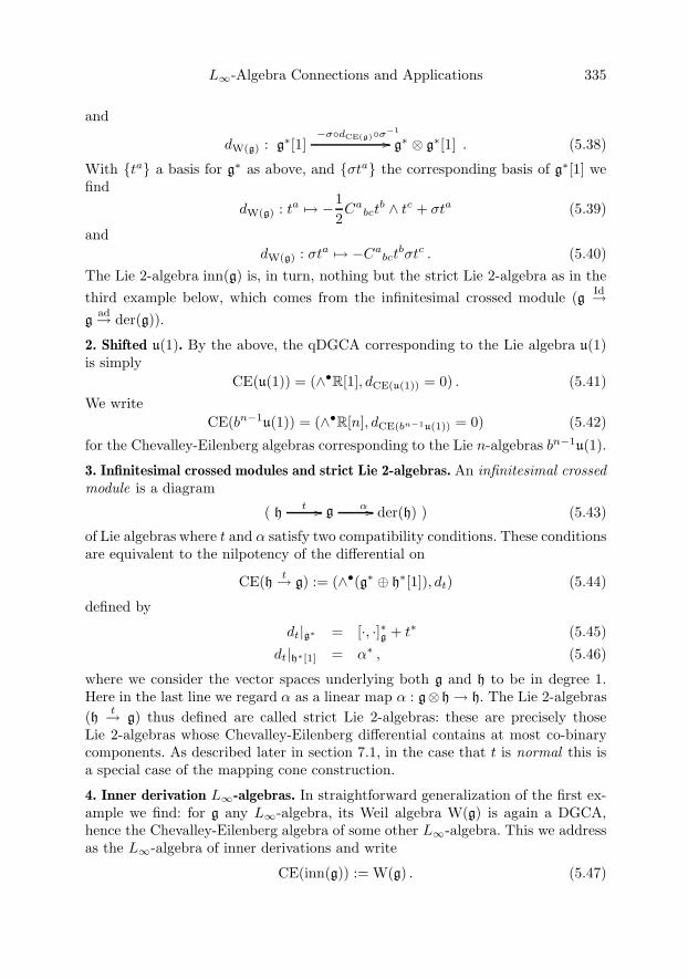
L∞-Algebra Connections and Applications 335
and
dW(g) : g∗[1]−σ◦dCE(g)◦σ−1
�� g∗ ⊗ g∗[1] . (5.38)
With {ta} a basis for g∗ as above, and {σta} the corresponding basis of g∗[1] wefind
dW(g) : ta �→ −12Ca
bctb ∧ tc + σta (5.39)
anddW(g) : σta �→ −Ca
bctbσtc . (5.40)
The Lie 2-algebra inn(g) is, in turn, nothing but the strict Lie 2-algebra as in thethird example below, which comes from the infinitesimal crossed module (g Id→g
ad→ der(g)).
2. Shifted u(1). By the above, the qDGCA corresponding to the Lie algebra u(1)is simply
CE(u(1)) = (∧•R[1], dCE(u(1)) = 0) . (5.41)We write
CE(bn−1u(1)) = (∧•R[n], dCE(bn−1u(1)) = 0) (5.42)
for the Chevalley-Eilenberg algebras corresponding to the Lie n-algebras bn−1u(1).
3. Infinitesimal crossed modules and strict Lie 2-algebras. An infinitesimal crossedmodule is a diagram
( ht �� g α �� der(h) ) (5.43)
of Lie algebras where t and α satisfy two compatibility conditions. These conditionsare equivalent to the nilpotency of the differential on
CE(h t→ g) := (∧•(g∗ ⊕ h∗[1]), dt) (5.44)
defined by
dt|g∗ = [·, ·]∗g + t∗ (5.45)
dt|h∗[1] = α∗ , (5.46)
where we consider the vector spaces underlying both g and h to be in degree 1.Here in the last line we regard α as a linear map α : g⊗ h → h. The Lie 2-algebras(h t→ g) thus defined are called strict Lie 2-algebras: these are precisely thoseLie 2-algebras whose Chevalley-Eilenberg differential contains at most co-binarycomponents. As described later in section 7.1, in the case that t is normal this isa special case of the mapping cone construction.
4. Inner derivation L∞-algebras. In straightforward generalization of the first ex-ample we find: for g any L∞-algebra, its Weil algebra W(g) is again a DGCA,hence the Chevalley-Eilenberg algebra of some other L∞-algebra. This we addressas the L∞-algebra of inner derivations and write
CE(inn(g)) := W(g) . (5.47)
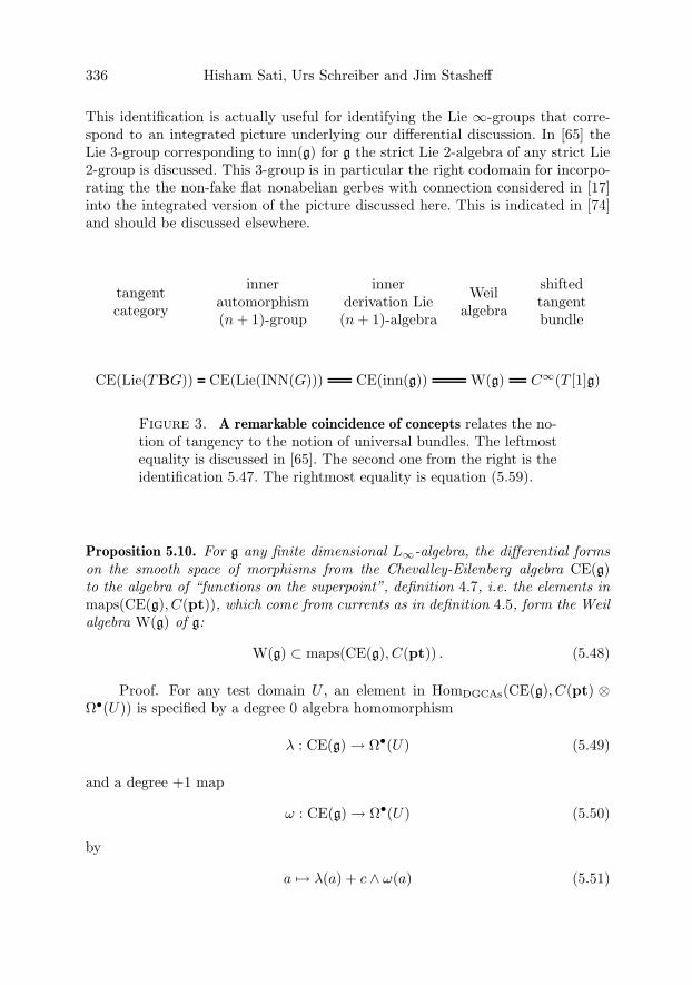
336 Hisham Sati, Urs Schreiber and Jim Stasheff
This identification is actually useful for identifying the Lie ∞-groups that corre-spond to an integrated picture underlying our differential discussion. In [65] theLie 3-group corresponding to inn(g) for g the strict Lie 2-algebra of any strict Lie2-group is discussed. This 3-group is in particular the right codomain for incorpo-rating the the non-fake flat nonabelian gerbes with connection considered in [17]into the integrated version of the picture discussed here. This is indicated in [74]and should be discussed elsewhere.
tangentcategory
innerautomorphism(n + 1)-group
innerderivation Lie(n + 1)-algebra
Weilalgebra
shiftedtangentbundle
CE(Lie(TBG)) CE(Lie(INN(G))) CE(inn(g)) W(g) C∞(T [1]g)
Figure 3. A remarkable coincidence of concepts relates the no-tion of tangency to the notion of universal bundles. The leftmostequality is discussed in [65]. The second one from the right is theidentification 5.47. The rightmost equality is equation (5.59).
Proposition 5.10. For g any finite dimensional L∞-algebra, the differential formson the smooth space of morphisms from the Chevalley-Eilenberg algebra CE(g)to the algebra of “functions on the superpoint”, definition 4.7, i.e. the elements inmaps(CE(g), C(pt)), which come from currents as in definition 4.5, form the Weilalgebra W(g) of g:
W(g) ⊂ maps(CE(g), C(pt)) . (5.48)
Proof. For any test domain U , an element in HomDGCAs(CE(g), C(pt) ⊗Ω•(U)) is specified by a degree 0 algebra homomorphism
λ : CE(g) → Ω•(U) (5.49)
and a degree +1 map
ω : CE(g) → Ω•(U) (5.50)
by
a �→ λ(a) + c ∧ ω(a) (5.51)

L∞-Algebra Connections and Applications 337
for all a ∈ g∗ and for c denoting the canonical degree -1 generator of C(pt); suchthat the equality in the bottom right corner of the diagram
a � dCE(g) ���
��
dCE(g)a�
��λ(a) + c ∧ ω(a) � dpt+dU �� λ(dCE(g)a)+c∧ω(dCE(g)a)
=d(λ(a))+ω(a)−c∧d(ω(a))
(5.52)
holds. Under the two canonical currents on C(pt) of degree 0 and degree 1, respec-tively, this gives rise for each a ∈ g∗ of degree |a| to an |a|-form and an (|a| + 1)form on maps(CE(g), C(pt)) whose values on a given plot are λ(a) and ω(a),respectively.
By the above diagram, the differential of these forms satisfies
dλ(a) = λ(dCE(g)a)− ω(a) (5.53)
anddω(a) = −ω(dCE(g)a) . (5.54)
But this is precisely the structure of W(g). �
To see the last step, it may be helpful to consider this for a simple case in termsof a basis:
let g be an ordinary Lie algebra, {ta} a basis of g∗ and {Cabc} the corre-
sponding structure constants. Then, using the fact that, since we are dealing withalgebra homomorphisms, we have
λ(ta ∧ tb) = λ(ta) ∧ λ(tb) (5.55)
andω(ta ∧ tb) = c ∧ (ω(ta) ∧ λ(tb)− λ(ta) ∧ ω(tb)) (5.56)
we finddλ(ta) = −1
2Ca
bcλ(tb) ∧ λ(tc)− ω(ta) (5.57)
anddω(ta) = −Ca
bcλ(tb) ∧ ω(tc) . (5.58)This is clearly just the structure of W(g).Remark. As usual, we may think of the superpoint as an “infinitesimal interval”.The above says that the algebra of inner derivations of an L∞-algebra consists ofthe maps from the infinitesimal interval to the supermanifold on which CE(g) isthe “algebra of functions”. On the one hand this tells us that
W(g) = C∞(T [1]g) (5.59)
in supermanifold language. On the other hand, this construction is clearly anal-ogous to the corresponding discussion for Lie n-groups given in [65]: there the3-group INN(G) of inner automorphisms of a strict 2-group G was obtained by
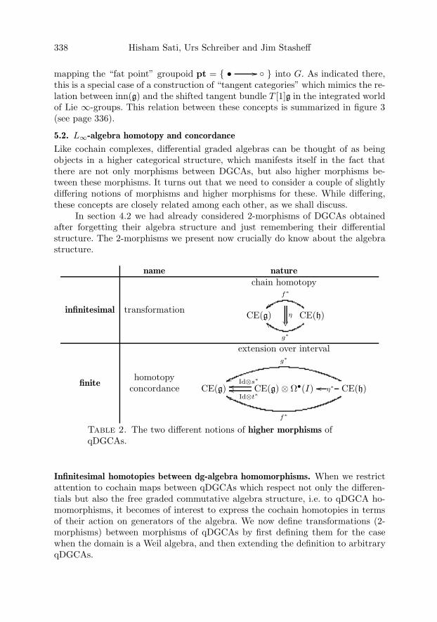
338 Hisham Sati, Urs Schreiber and Jim Stasheff
mapping the “fat point” groupoid pt = { • �� ◦ } into G. As indicated there,this is a special case of a construction of “tangent categories” which mimics the re-lation between inn(g) and the shifted tangent bundle T [1]g in the integrated worldof Lie ∞-groups. This relation between these concepts is summarized in figure 3(see page 336).
5.2. L∞-algebra homotopy and concordance
Like cochain complexes, differential graded algebras can be thought of as beingobjects in a higher categorical structure, which manifests itself in the fact thatthere are not only morphisms between DGCAs, but also higher morphisms be-tween these morphisms. It turns out that we need to consider a couple of slightlydiffering notions of morphisms and higher morphisms for these. While differing,these concepts are closely related among each other, as we shall discuss.
In section 4.2 we had already considered 2-morphisms of DGCAs obtainedafter forgetting their algebra structure and just remembering their differentialstructure. The 2-morphisms we present now crucially do know about the algebrastructure.
name nature
infinitesimal transformation
chain homotopy
CE(g) CE(h)
g∗
��
f∗
η
finitehomotopy
concordance
extension over interval
CE(g) CE(g)⊗ Ω•(I)Id⊗t∗
��Id⊗s∗
�� CE(h)η∗��
g∗
��
f∗
��
Table 2. The two different notions of higher morphisms ofqDGCAs.
Infinitesimal homotopies between dg-algebra homomorphisms. When we restrictattention to cochain maps between qDGCAs which respect not only the differen-tials but also the free graded commutative algebra structure, i.e. to qDGCA ho-momorphisms, it becomes of interest to express the cochain homotopies in termsof their action on generators of the algebra. We now define transformations (2-morphisms) between morphisms of qDGCAs by first defining them for the casewhen the domain is a Weil algebra, and then extending the definition to arbitraryqDGCAs.
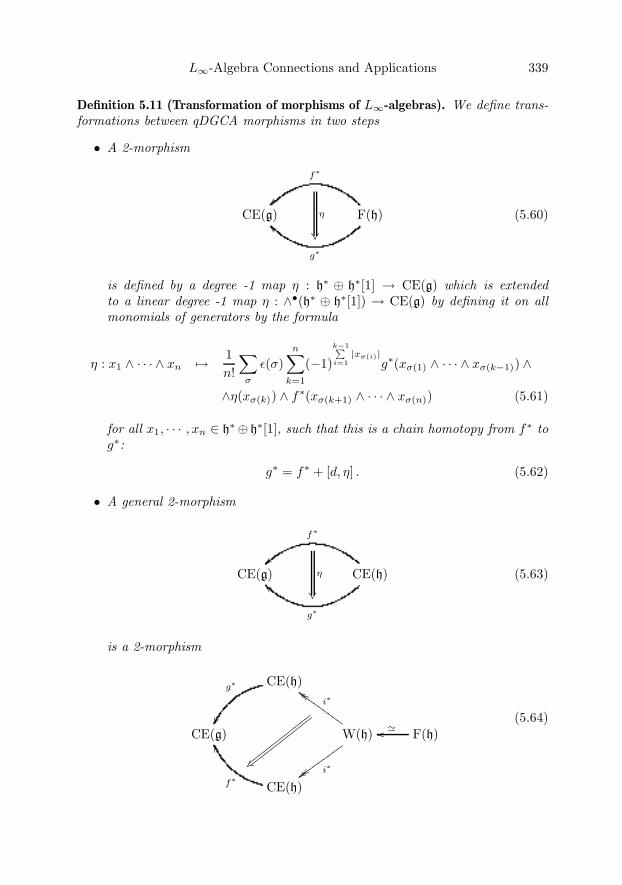
L∞-Algebra Connections and Applications 339
Definition 5.11 (Transformation of morphisms of L∞-algebras). We define trans-formations between qDGCA morphisms in two steps
• A 2-morphism
CE(g) F(h)
g∗
��
f∗
��η
(5.60)
is defined by a degree -1 map η : h∗ ⊕ h∗[1] → CE(g) which is extendedto a linear degree -1 map η : ∧•(h∗ ⊕ h∗[1]) → CE(g) by defining it on allmonomials of generators by the formula
η : x1 ∧ · · · ∧ xn �→ 1n!
∑σ
ε(σ)n∑
k=1
(−1)k−1∑i=1
|xσ(i)|g∗(xσ(1) ∧ · · · ∧ xσ(k−1)) ∧
∧η(xσ(k)) ∧ f∗(xσ(k+1) ∧ · · · ∧ xσ(n)) (5.61)
for all x1, · · · , xn ∈ h∗⊕ h∗[1], such that this is a chain homotopy from f∗ tog∗:
g∗ = f∗ + [d, η] . (5.62)
• A general 2-morphism
CE(g) CE(h)
g∗
��
f∗
η
(5.63)
is a 2-morphism
CE(h)g∗
��CE(g) W(h)
i∗����
i∗����������
���
F(h)���
CE(h)f∗
��
� ������������
������������ (5.64)

340 Hisham Sati, Urs Schreiber and Jim Stasheff
of the above kind that vanishes on the shifted generators, i.e. such that
CE(h)g∗
��CE(g) W(h)
i∗����
i∗������������
�h∗[1]� ���
CE(h)f∗
��
� ������������
������������ (5.65)
vanishes.
Proposition 5.12. Formula 5.61 is consistent in that g∗|h∗⊕h∗[1] =(f∗ + [d, η])|h∗⊕h∗[1] implies that g∗ = f∗ + [d, η] on all elements of F (h).
Remark. Definition 5.11, which may look ad hoc at this point, has a practical anda deep conceptual motivation.
• Practical motivation. While it is clear that 2-morphisms of qDGCAs shouldbe chain homotopies, it is not straightforward, in general, to characterizethese by their action on generators. Except when the domain qDGCA is free,in which case our formula (5.11) makes sense. The prescription (5.64) thenprovides a systematic algorithm for extending this to arbitrary qDGCAs.
In particular, using the isomorphism W(g) � F(g) from proposition 5.7,the above yields the usual explicit description of the homotopy operator τ :W(g) → W(g) with IdW(g) = [dW(g), τ ]. Among other things, this computesfor us the transgression elements (“Chern-Simons elements”) for L∞-algebrasin section 5.3.
• Conceptual motivation. As we will see in sections 5.3 and 5.5, the qDGCAW(g) plays an important twofold role: it is both the algebra of differentialforms on the total space of the universal g-bundle – while CE(g) is that offorms on the fiber –, as well as the domain for g-valued differential forms,where the shifted component, that in g∗[1], is the home of the correspondingcurvature.
In the light of this, the above restriction (5.65) can be understood assaying either that
– vertical transformations induce transformations on the fibers;or
– gauge transformations of g-valued forms are transformations underwhich the curvatures transform covariantly.
Finite transformations between qDGCA morphisms: concordances. We now con-sider the finite transformations of morphisms of DGCAs. What we called 2-mor-phisms or transformations for qDGCAs above would in other contexts possibly becalled a homotopy. Also the following concept is a kind of homotopy, and appearsas such in [75] which goes back to [14]. Here we wish to clearly distinguish these
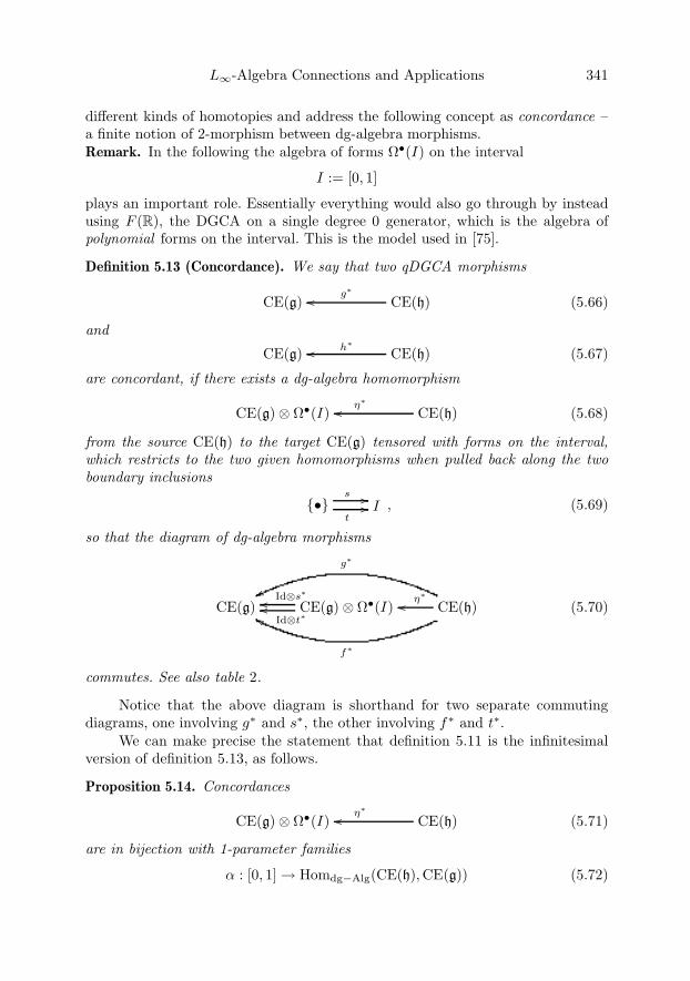
L∞-Algebra Connections and Applications 341
different kinds of homotopies and address the following concept as concordance –a finite notion of 2-morphism between dg-algebra morphisms.Remark. In the following the algebra of forms Ω•(I) on the interval
I := [0, 1]
plays an important role. Essentially everything would also go through by insteadusing F (R), the DGCA on a single degree 0 generator, which is the algebra ofpolynomial forms on the interval. This is the model used in [75].
Definition 5.13 (Concordance). We say that two qDGCA morphisms
CE(g) CE(h)g∗
�� (5.66)
and
CE(g) CE(h)h∗�� (5.67)
are concordant, if there exists a dg-algebra homomorphism
CE(g)⊗ Ω•(I) CE(h)η∗
�� (5.68)
from the source CE(h) to the target CE(g) tensored with forms on the interval,which restricts to the two given homomorphisms when pulled back along the twoboundary inclusions
{•}s ��t
�� I , (5.69)
so that the diagram of dg-algebra morphisms
CE(g) CE(g)⊗ Ω•(I)Id⊗t∗
��Id⊗s∗
�� CE(h)η∗
��
g∗
��
f∗
��(5.70)
commutes. See also table 2.
Notice that the above diagram is shorthand for two separate commutingdiagrams, one involving g∗ and s∗, the other involving f∗ and t∗.
We can make precise the statement that definition 5.11 is the infinitesimalversion of definition 5.13, as follows.
Proposition 5.14. Concordances
CE(g)⊗ Ω•(I) CE(h)η∗
�� (5.71)
are in bijection with 1-parameter families
α : [0, 1] → Homdg−Alg(CE(h),CE(g)) (5.72)

342 Hisham Sati, Urs Schreiber and Jim Stasheff
of morphisms whose derivatives with respect to the parameter is a chain homotopy,i.e. a 2-morphism
∀t ∈ [0, 1] : CE(g) CE(h)
ddt α(t)=[d,ρ]
��
0
ρ
(5.73)
in the 2-category of cochain complexes. For any such α, the morphisms f∗ andg∗ between which it defines a concordance are defined by the value of α on theboundary of the interval.
Proof. Writing t : [0, 1] → R for the canonical coordinate function on theinterval I = [0, 1] we can decompose the dg-algebra homomorphism η∗ as
η∗ : ω �→ (t �→ α(ω)(t) + dt ∧ ρ(ω)(t)) . (5.74)
α is itself a degree 0 dg-algebra homomorphism, while ρ is degree -1 map. Thenthe fact that η∗ respects the differentials implies that for all ω ∈ CE(h) we have
ω � dh ���
η∗
��
dhω�
η∗
��
(t �→ (α(ω)(t) + dt ∧ ρ(ω)(t))) � dg+dt��(t �→ (α(dhω)(t) + dt ∧ ρ(dhω)(t))= (t �→ (dg(α(ω))(t)+dt ∧ ( d
dtα(ω)− dgρ(ω))(t))(5.75)
The equality in the bottom right corner says that
α ◦ dh − dg ◦ α = 0 (5.76)
and
∀ω ∈ CE(g) :d
dtα(ω) = ρ(dhω) + dg(ρ(ω)) . (5.77)
But this means that α is a chain homomorphism whose derivative is given by achain homotopy. �
5.2.1. Examples.Transformations between DGCA morphisms. We demonstrate two examples forthe application of the notion of transformations of DGCA morphisms from defini-tion 5.11 which are relevant for us.

L∞-Algebra Connections and Applications 343
Computation of transgression forms. As an example for the transformation in def-inition 5.11, we show how the usual Chern-Simons transgression form is computedusing formula (5.61). The reader may wish to first skip to our discussion of Lie ∞-algebra cohomology in section 5.3 for more background. So let g be an ordinary Liealgebra with invariant bilinear form P , which we regard as a dW(g)-closed elementP ∈ ∧2g∗[1] ⊂ W(g). We would like to compute τP , where τ is the contractinghomotopy of W(g), such that
[d, τ ] = IdW(g) , (5.78)
which according to proposition 5.7 is given on generators by
τ : a �→ 0 (5.79)τ : dW(g)a �→ a (5.80)
for all a ∈ g∗. Let {ta} be a chosen basis of g∗ and let {Pab} be the componentsof P in that basis, then
P = Pab(σta) ∧ (σtb) . (5.81)
In order to apply formula (5.61) we need to first rewrite this in terms of monomialsin {ta} and {dW(g)t
a}. Hence, using σta = dW(g)ta + 1
2Ca
bctb ∧ tc, we get
τP = τ(Pab(dW(g)t
a) ∧ (dW(g)ta)− Pab(dW(g)t
a) ∧Cbcdt
c ∧ td
+14PabC
acdC
bef t
c ∧ td ∧ tc ∧ td). (5.82)
Now equation (5.61) can be applied to each term. Noticing the combinatorialprefactor 1
n! , which depends on the number of factors in the above terms, andnoticing the sum over all permutations, we find
τ(Pab(dW(g)t
a) ∧ (dW(g)ta))
= Pab(dW(g)ta) ∧ tb
τ(−Pab(dW(g)t
a) ∧ Cbcdt
c ∧ td)
=13!· 2 PabC
bcdt
b ∧ tc ∧ td
=13Cabct
a ∧ tb ∧ tc (5.83)
where we write Cabc := PadCd
bc as usual. Finally τ(
14PabC
acdC
bef t
c ∧ td ∧ tc ∧ td)
= 0 . In total this yields
τP = Pab(dW(g)ta) ∧ tb +
13Cabct
a ∧ tb ∧ tc . (5.84)
By again using dW(g)ta = − 1
2Ca
bctb ∧ tc + σta together with the invariance of P
(hence the dW(g)-closedness of P which implies that the constants Cabc are skewsymmetric in all three indices), one checks that this does indeed satisfy
dW(g)τP = P . (5.85)
In section 5.5 we will see that after choosing a g-valued connection on the space Ythe generators ta here will get sent to components of a g-valued 1-form A, while
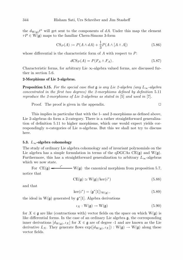
344 Hisham Sati, Urs Schreiber and Jim Stasheff
the dW(g)ta will get sent to the components of dA. Under this map the element
τP ∈ W(g) maps to the familiar Chern-Simons 3-form
CSP (A) := P (A ∧ dA) +13P (A ∧ [A ∧A]) (5.86)
whose differential is the characteristic form of A with respect to P :
dCSP (A) = P (FA ∧ FA) . (5.87)
Characteristic forms, for arbitrary Lie ∞-algebra valued forms, are discussed fur-ther in section 5.6.
2-Morphisms of Lie 2-algebras.
Proposition 5.15. For the special case that g is any Lie 2-algebra (any L∞-algebraconcentrated in the first two degrees) the 2-morphisms defined by definition 5.11reproduce the 2-morphisms of Lie 2-algebras as stated in [5] and used in [7].
Proof. The proof is given in the appendix. �
This implies in particular that with the 1- and 2-morphisms as defined above,Lie 2-algebras do form a 2-category. There is a rather straightforward generaliza-tion of definition 5.11 to higher morphisms, which one would expect yields cor-respondingly n-categories of Lie n-algebras. But this we shall not try to discusshere.
5.3. L∞-algebra cohomology
The study of ordinary Lie algebra cohomology and of invariant polynomials on theLie algebra has a simple formulation in terms of the qDGCAs CE(g) and W(g).Furthermore, this has a straightforward generalization to arbitrary L∞-algebraswhich we now state.
For CE(g) W(g)i∗���� the canonical morphism from proposition 5.7,notice that
CE(g) � W(g)/ker(i∗) (5.88)
and thatker(i∗) = 〈g∗[1]〉W(g) , (5.89)
the ideal in W(g) generated by g∗[1]. Algebra derivations
ιX : W(g) → W(g) (5.90)
for X ∈ g are like (contractions with) vector fields on the space on which W(g) islike differential forms. In the case of an ordinary Lie algebra g, the correspondinginner derivations [dW(g), ιX ] for X ∈ g are of degree -1 and are known as the Liederivative LX . They generate flows exp([dW(g), ιX ]) : W(g) → W(g) along thesevector fields.

L∞-Algebra Connections and Applications 345
Definition 5.16 (Vertical derivations). We say an algebra derivation τ : W(g) →W(g) is vertical if it vanishes on the shifted copy g∗[1] of g∗ inside W(g),
τ |g∗[1] = 0 . (5.91)
Proposition 5.17. The vertical derivations are precisely those that come from con-tractions
ιX : g∗ �→ R (5.92)for all X ∈ g, extended to 0 on g∗[1] and extended as algebra derivations to all of∧•(g∗ ⊕ g∗[1]).
The reader should compare this and the following definitions to the theory ofvertical Lie derivatives and basic differential forms with respect to any surjectivesubmersion π : Y → X . This is discussed in section 4.3.1.
Definition 5.18 (Basic forms and invariant polynomials). The algebra W(g)basic ofbasic forms in W(g) is the intersection of the kernels of all vertical derivations andLie derivatives. i.e. all the contractions ιX and Lie derivatives LX for X ∈ g. SinceLX = [dW(g), ιX ], it follows that in the kernel of ιX , the Lie derivative vanishesonly if ιXdW(g) vanishes.
As will be discussed in a moment, basic forms in W(g) play the role of in-variant polynomials on the L∞-algebra g. Therefore we often write inv(g) forW(g)basic:
inv(g) := W(g)basic . (5.93)
Using the obvious inclusion W(g) inv(g)� �p∗
�� we obtain the sequence
CE(g) W(g)i∗���� inv(g)� �p∗
�� (5.94)
of dg-algebras that plays a major role in our analysis: it can be interpreted ascoming from the universal bundle for the Lie ∞-algebra g. As shown in figure 4,we can regard vertical derivations on W(g) as derivations along the fibers of thecorresponding dual sequence.
Definition 5.19 (Cocycles, invariant polynomials and transgression elements). Letg be an L∞-algebra. Then• An L∞-algebra cocycle on g is a dCE(g)-closed element of CE(g).
μ ∈ CE(g) , dCE(g)μ = 0 . (5.95)
• An L∞-algebra invariant polynomial on g is an element P ∈ inv(g) :=W(g)basic.
• An L∞-algebra g-transgression element for a given cocycle μ and an invariantpolynomial P is an element cs ∈ W(g) such that
dW(g)cs = p∗P (5.96)
i∗cs = μ . (5.97)
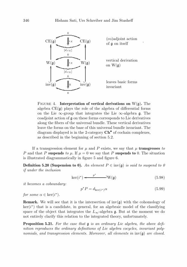
346 Hisham Sati, Urs Schreiber and Jim Stasheff
CE(g) CE(g)
[d,ιX ]
��
0
�� (co)adjoint actionof g on itself
W(g)
����
W(g)
����
[d,ιX ]
��
0
�� vertical derivationon W(g)
inv(g)��
��
inv(g)��
��
0
��
0
�� leaves basic formsinvariant
ιX
0
ιX
.
Figure 4. Interpretation of vertical derivations on W(g). Thealgebra CE(g) plays the role of the algebra of differential formson the Lie ∞-group that integrates the Lie ∞-algebra g. Thecoadjoint action of g on these forms corresponds to Lie derivativesalong the fibers of the universal bundle. These vertical derivativesleave the forms on the base of this universal bundle invariant. Thediagram displayed is in the 2-category Ch• of cochain complexes,as described in the beginning of section 5.2.
If a transgression element for μ and P exists, we say that μ transgresses toP and that P suspends to μ. If μ = 0 we say that P suspends to 0. The situationis illustrated diagrammatically in figure 5 and figure 6.
Definition 5.20 (Suspension to 0). An element P ∈ inv(g) is said to suspend to 0if under the inclusion
ker(i∗) W(g)� �p∗
�� (5.98)
it becomes a coboundary:p∗P = dker(i∗)α (5.99)
for some α ∈ ker(i∗).
Remark. We will see that it is the intersection of inv(g) with the cohomology ofker(i∗) that is a candidate, in general, for an algebraic model of the classifyingspace of the object that integrates the L∞-algebra g. But at the moment we donot entirely clarify this relation to the integrated theory, unfortunately.
Proposition 5.21. For the case that g is an ordinary Lie algebra, the above defi-nition reproduces the ordinary definitions of Lie algebra cocycles, invariant poly-nomials, and transgression elements. Moreover, all elements in inv(g) are closed.

L∞-Algebra Connections and Applications 347
cocycle transgression element inv. polynomial
G� � i �� EG
p �� �� BG
0
0 p∗P�
d
��
P�
p∗��
μ�
d
��
cs�i∗
�� �d
��
Figure 5. Lie algebra cocycles, invariant polynomials and trans-gression forms in terms of cohomology of the universal G-bundle.Let G be a simply connected compact Lie group with Lie al-gebra g. Then invariant polynomials P on g correspond to ele-ments in the cohomology H•(BG) of the classifying space of G.When pulled back to the total space of the universal G-bundleEG→ BG, these classes become trivial, due to the contractabil-ity of EG: p∗P = d(cs). Lie algebra cocycles, on the other hand,correspond to elements in the cohomology H•(G) of G itself. A co-cycle μ ∈ H•(G) is in transgression with an invariant polynomialP ∈ H•(BG) if μ = i∗cs.
Proof. That the definitions of Lie algebra cocycles and transgression ele-ments coincides is clear. It remains to be checked that inv(g) really contains theinvariant polynomials. In the ordinary definition a g-invariant polynomial is adW(g)-closed element in ∧•(g∗[1]). Hence one only needs to check that all elementsin ∧•(g∗[1]) with the property that their image under dW(g) is again in ∧•(g∗[1])are in fact already closed. This can be seen for instance in components, using thedescription of W(g) given in section 5.1.1. �
Remark. For ordinary Lie algebras g corresponding to a simply connected compactLie group G, the situation is often discussed in terms of the cohomology of theuniversal G-bundle. This is recalled in figure 5 and in section 5.3.1. The generaldefinition above is a precise analog of that familiar situation: W(g) plays the roleof the algebra of (left invariant) differential forms on the universal g-bundle andCE(g) plays the role of the algebra of (left invariant) differential forms on its fiber.Then inv(g) plays the role of differential forms on the base, BG = EG/G. In fact,

348 Hisham Sati, Urs Schreiber and Jim Stasheff
cocycle transgression element inv. polynomial
CE(g) W(g)i∗���� inv(g)� �p∗
��
0
0 p∗P�
dW(g)
��
τ
��
P�
p∗��
μ�
dCE(g)
��
cs�i∗�� �dW(g)
��
Figure 6. The homotopy operator τ is a contraction homotopyfor W(g). Acting with it on a closed invariant polynomial P ∈inv(g) ⊂ ∧•g[1] ⊂ W(g) produces an element cs ∈ W (g) whose“restriction to the fiber” μ := i∗cs is necessarily closed and hencea cocycle. We say that cs induces the transgression from μ to P ,or that P suspends to μ.
for G a compact and simply connected Lie group and g its Lie algebra, we have
H•(inv(g)) � H•(BG,R) . (5.100)
In summary, the situation we thus obtain is that depicted in figure 1. Comparethis to the following fact.
Proposition 5.22. For p : P → X a principal G-bundle, let vert(P ) ⊂ Γ(TP ) bethe vertical vector fields on P . The horizontal differential forms on P which areinvariant under vert(P ) are precisely those that are pulled back along p from X.
These are called the basic differential forms in [41].Remark. We will see that, contrary to the situation for ordinary Lie algebras,in general invariant polynomials of L∞ algebras are not dW(g)-closed (the dW(g)-differential of them is just horizontal). We will also see that those indecomposableinvariant polynomials in inv(g), i.e. those that become exact in ker(i∗), are notcharacteristic for the corresponding g-bundles. This probably means that the realcohomology of the classifying space of the Lie ∞-group integrating g is spanned byinvariant polynomials modulo those suspending to 0. But here we do not attemptto discuss this further.
Proposition 5.23. For every invariant polynomial P ∈ ∧•g[1] ⊂ W(g) on an L∞-algebra g such that dW(g)p
∗P = 0, there exists an L∞-algebra cocycle μ ∈ CS(g)that transgresses to P .
L∞-Algebra Connections and Applications 349
Proof. This is a consequence of proposition 5.7 and proposition 5.8. LetP ∈ W (g) be an invariant polynomial. By proposition 5.7, p∗P is in the kernel
of the restriction homomorphism CE(g) W(g)i∗���� : i∗P = 0. By proposition5.8, p∗P is the image under dW(g) of an element cs := τ(p∗P ) and by the algebrahomomorphism property of i∗ we know that its restriction, μ := i∗cs, to the fiberis closed, because
dCE(g)i∗cs = i∗dW(g)cs = i∗p∗P = 0 . (5.101)
Therefore μ is an L∞-algebra cocycle for g that transgresses to the invariant poly-nomial P . �
Remark. Notice that this statement is useful only for indecomposable invariantpolynomials. All others trivially suspend to the 0 cocycle.
Proposition 5.24. An invariant polynomial which suspends to a Lie ∞-algebracocycle that is a coboundary also suspends to 0.
Proof. Let P be an invariant polynomial, cs the corresponding transgres-sion element and μ = i∗cs the corresponding cocycle, which is assumed to be acoboundary in that μ = dCE(g)b for some b ∈ CE(g). Then by the definition ofdW(g) it follows that μ = i∗(dW(g)b).
Now notice thatcs′ := cs− dW(g)b (5.102)
is another transgression element for P , since
dW(g)cs′ = p∗P . (5.103)
But nowi∗(cs′) = i∗(cs− dW(g)b) = 0 . (5.104)
Hence P suspends to 0. �
5.3.1. Examples.The cohomologies of G and of BG in terms of qDGCAs. To put our generalconsiderations for L∞-algebras into perspective, it is useful to keep the followingclassical results for ordinary Lie algebras in mind.
A classical result of E. Cartan [22] [23] (see also [49]) says that for a connectedfinite dimensional Lie group G, the cohomology H•(G) of the group is isomorphicto that of the Chevalley-Eilenberg algebra CE(g) of its Lie algebra g:
H•(G) � H•(CE(g)) , (5.105)
namely to the algebra of Lie algebra cocycles on g. If we denote by QG the spaceof indecomposable such cocycles, and form the qDGCA ∧•QG = H•(∧•QG) withtrivial differential, the above says that we have an isomorphism in cohomology
H•(G) � H•(∧•QG) = ∧•QG (5.106)

350 Hisham Sati, Urs Schreiber and Jim Stasheff
which is realized by the canonical inclusion
i : ∧•QG� � �� CE(g) (5.107)
of all cocycles into the Chevalley-Eilenberg algebra.Subsequently, we have the classical result of Borel [13]: For a connected finite
dimensional Lie group G, the cohomology of its classifying space BG is a finitelygenerated polynomial algebra on even dimensional generators:
H•(BG) � ∧•PG . (5.108)
Here PG is the space of indecomposable invariant polynomials on g, hence
H•(BG) � H•(inv(g)) . (5.109)
In fact, PG and QG are isomorphic after a shift:
PG � QG[1] (5.110)
and this isomorphism is induced by transgression between indecomposable co-cycles μ ∈ CE(g) and indecomposable invariant polynomials P ∈ inv(g) via atransgression element cs = τP ∈ W(g).Cohomology and invariant polynomials of bn−1u(1).
Proposition 5.25. For every integer n ≥ 1, the Lie n-algebra bn−1u(1) (the (n−1)-folded shifted version of ordinary u(1)) from section 5.1.1) we have the following:
• there is, up to a scalar multiple, a single indecomposable Lie∞-algebra cocyclewhich is of degree n and linear,
μbn−1u(1) ∈ R[n] ⊂ CE(bn−1u(1)) , (5.111)
• there is, up to a scalar multiple, a single indecomposable Lie ∞-algebra in-variant polynomial, which is of degree (n + 1)
Pbn−1u(1) ∈ R[n + 1] ⊂ inv(bn−1u(1)) = CE(bnu(1)) . (5.112)
• The cocycle μbn−1u(1) is in transgression with Pbn−1u(1).
These statements are an obvious consequence of the definitions involved, butthey are important. The fact that bn−1u(1) has a single invariant polynomial ofdegree (n + 1) will immediately imply, in section 6, that bn−1u(1)-bundles havea single characteristic class of degree (n + 1): known (at least for n = 2, as theDixmier-Douady class). Such a bn−1u(1)-bundle classes appear in 7 as the obstruc-tion classes for lifts of n-bundles through String-like extensions of their structureLie n-algebra.

L∞-Algebra Connections and Applications 351
Cohomology and invariant polynomials of strict Lie 2-algebras. Let g(2) = (h t→g
α→ der(h)) be a strict Lie 2-algebra as described in section 5.1. Notice that thereis a canonical projection homomorphism
CE(g) CE(h t→ g)j∗���� (5.113)
which, of course, extends to the Weil algebras
W(g) W(h t→ g)j∗���� . (5.114)
Here j∗ is simply the identity on g∗ and on g∗[1] and vanishes on h∗[1] and h∗[2].
Proposition 5.26. Every invariant polynomial P ∈ inv(g) of the ordinary Lie alge-bra g lifts to an invariant polynomial on the Lie 2-algebra (h t→ g):
W(h t→ g)
i∗
����W(g) inv(g)� ���
� �
��
. (5.115)
However, a closed invariant polynomial will not necessarily lift to a closed one.
Proof. Recall that dt := dCE(h
t→g)acts on g∗ as
dt|g∗ = [·, ·]∗g + t∗ . (5.116)
By definition 5.4 and definition 5.5 it follows that dW(h
t→g)acts on g∗[1] as
dW(h
t→g)|g∗[1] = −σ ◦ [·, ·]∗g − σ ◦ t∗ (5.117)
and on h∗[1] as
dW(h
t→g)|h∗[1] = −σ ◦ α∗ . (5.118)
Then notice that
(σ ◦ t∗) : g∗[1] → h∗[2] . (5.119)
But this means that dW(h
t→g)differs from dW(g) on ∧•(g∗[1]) only by elements that
are annihilated by vertical ιX . This proves the claim. �
It may be easier to appreciate this proof by looking at what it does in termsof a chosen basis.
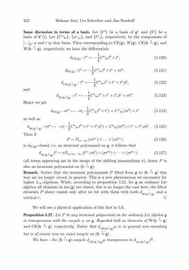
352 Hisham Sati, Urs Schreiber and Jim Stasheff
Same discussion in terms of a basis. Let {ta} be a basis of g∗ and {bi} be abasis of h∗[1]. Let {Ca
bc}, {αiaj}, and {tai}, respectively, be the components of
[·, ·]g, α and t in that basis. Then corresponding to CE(g), W(g), CE(h t→ g), andW(h t→ g), respectively, we have the differentials
dCE(g) : ta �→ −12Ca
bctb ∧ tc, (5.120)
dW(g) : ta �→ −12Ca
bctb ∧ tc + σta, (5.121)
dCE(h
t→g): ta �→ −1
2Ca
bctb ∧ tc + taib
i, (5.122)
anddW(h
t→g): ta �→ −1
2Ca
bctb ∧ tc + taib
i + σta. (5.123)
Hence we get
dW(g) : σta �→ −σ(−12Ca
bctb ∧ tc) = Ca
bc(σtb) ∧ tc (5.124)
as well as
dW(h
t→g): σta �→ −σ(−1
2Ca
bctb ∧ tc + taib
i) = Cabc(σtb) ∧ tc + taiσb
i . (5.125)
Then ifP = Pa1···an(σta1) ∧ · · · ∧ (σtan) (5.126)
is dW(g)-closed, i.e. an invariant polynomial on g, it follows that
dW(h
t→g)P = nPa1,a2,···an(ta1
iσbi) ∧ (σta2 ) ∧ · · · ∧ (σtan) . (5.127)
(all terms appearing are in the image of the shifting isomorphism σ), hence P isalso an invariant polynomial on (h t→ g).Remark. Notice that the invariant polynomials P lifted from g to (h t→ g) thisway are no longer closed, in general. This is a new phenomenon we encounter forhigher L∞-algebras. While, according to proposition 5.21, for g an ordinary Liealgebra all elements in inv(g) are closed, this is no longer the case here: the liftedelements P above vanish only after we hit with them with both d
W(ht→g)
and avertical τ . �
We will see a physical application of this fact in 5.6.
Proposition 5.27. Let P be any invariant polynomial on the ordinary Lie algebra g
in transgression with the cocycle μ on g. Regarded both as elements of W(h t→ g)and CE(h t→ g) respectively. Notice that d
CE(ht→g)
μ is in general non-vanishing
but is of course now an exact cocycle on (h t→ g).We have : the (h t→ g)-cocycle d
CE(ht→g)
μ transgresses to dinv(h
t→g)P .

L∞-Algebra Connections and Applications 353
0
0 p∗dinv(h
t→g)P
�
τW(h t→g)
��
�
dW(h t→g)
��
dinv(h
t→g)P�
p∗W(h t→g)��
dCE(h
t→g)μ
�
dCE(h t→g)
��
τp∗dinv(h
t→g)P
�
dW(h t→g)
��
�i∗�� P�
dinv(h t→g)
��
.
Figure 7. Cocycles and invariant polynomials on strict Lie 2-
algebras (h t→ g), induced from cocycles and invariant polynomi-als on g. An invariant polynomial P on g in transgression with acocycle μ on g lifts to a generally non-closed invariant polynomialon (h t→ g). The diagram says that its closure, d
inv(ht→g)
P , sus-
pends to the dCE(h
t→g)-closure of the cocycle μ. Since this (h t→ g)-
cocycle d(h
t→g)μ is hence a coboundary, it follows from proposition
5.24 that dinv(h
t→g)P suspends also to 0. Nevertheless the situa-
tion is of interest, in that it governs the topological field theoryknown as BF theory. This is discussed in section 5.6.1.
The situation is illustrated by the diagram in figure 7.
Concrete Example: su(5) → sp(5). It is known that the cohomology of theChevalley-Eilenberg algebras for su(5) and sp(5) are generated, respectively, byfour and five indecomposable cocycles,
H•(CE(su(5))) = ∧•[a, b, c, d] (5.128)
and
H•(CE(sp(5))) = ∧•[v, w, x, y, z] , (5.129)
which have degree as indicated in the following table:
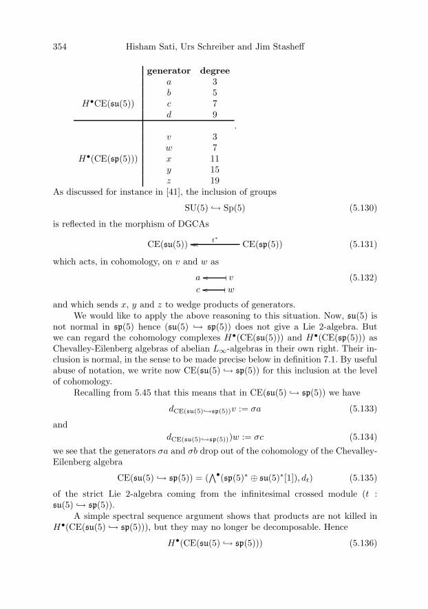
354 Hisham Sati, Urs Schreiber and Jim Stasheff
generator degreea 3b 5
H•CE(su(5)) c 7d 9
v 3w 7
H•(CE(sp(5))) x 11y 15z 19
.
As discussed for instance in [41], the inclusion of groups
SU(5) ↪→ Sp(5) (5.130)
is reflected in the morphism of DGCAs
CE(su(5)) CE(sp(5))t∗���� (5.131)
which acts, in cohomology, on v and w as
a v���
c w���(5.132)
and which sends x, y and z to wedge products of generators.We would like to apply the above reasoning to this situation. Now, su(5) is
not normal in sp(5) hence (su(5) ↪→ sp(5)) does not give a Lie 2-algebra. Butwe can regard the cohomology complexes H•(CE(su(5))) and H•(CE(sp(5))) asChevalley-Eilenberg algebras of abelian L∞-algebras in their own right. Their in-clusion is normal, in the sense to be made precise below in definition 7.1. By usefulabuse of notation, we write now CE(su(5) ↪→ sp(5)) for this inclusion at the levelof cohomology.
Recalling from 5.45 that this means that in CE(su(5) ↪→ sp(5)) we have
dCE(su(5)↪→sp(5))v := σa (5.133)
anddCE(su(5)↪→sp(5)))w := σc (5.134)
we see that the generators σa and σb drop out of the cohomology of the Chevalley-Eilenberg algebra
CE(su(5) ↪→ sp(5)) = (∧•(sp(5)∗ ⊕ su(5)∗[1]), dt) (5.135)
of the strict Lie 2-algebra coming from the infinitesimal crossed module (t :su(5) ↪→ sp(5)).
A simple spectral sequence argument shows that products are not killed inH•(CE(su(5) ↪→ sp(5))), but they may no longer be decomposable. Hence
H•(CE(su(5) ↪→ sp(5))) (5.136)
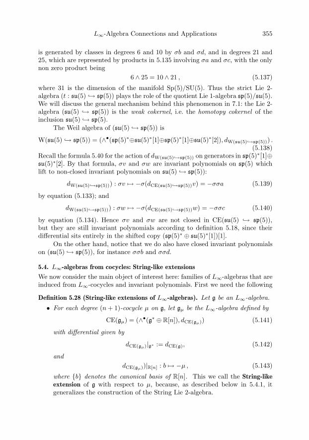
L∞-Algebra Connections and Applications 355
is generated by classes in degrees 6 and 10 by σb and σd, and in degrees 21 and25, which are represented by products in 5.135 involving σa and σc, with the onlynon zero product being
6 ∧ 25 = 10 ∧ 21 , (5.137)
where 31 is the dimension of the manifold Sp(5)/SU(5). Thus the strict Lie 2-algebra (t : su(5) ↪→ sp(5)) plays the role of the quotient Lie 1-algebra sp(5)/su(5).We will discuss the general mechanism behind this phenomenon in 7.1: the Lie 2-algebra (su(5) ↪→ sp(5)) is the weak cokernel, i.e. the homotopy cokernel of theinclusion su(5) ↪→ sp(5).
The Weil algebra of (su(5) ↪→ sp(5)) is
W(su(5) ↪→ sp(5)) = (∧•(sp(5)∗⊕su(5)∗[1]⊕sp(5)∗[1]⊕su(5)∗[2]), dW(su(5)↪→sp(5))) .(5.138)
Recall the formula 5.40 for the action of dW(su(5)↪→sp(5)) on generators in sp(5)∗[1]⊕su(5)∗[2]. By that formula, σv and σw are invariant polynomials on sp(5) whichlift to non-closed invariant polynomials on su(5) ↪→ sp(5)):
dW(su(5)↪→sp(5))) : σv �→ −σ(dCE(su(5)↪→sp(5))v) = −σσa (5.139)
by equation (5.133); and
dW(su(5)↪→sp(5))) : σw �→ −σ(dCE(su(5)↪→sp(5))w) = −σσc (5.140)
by equation (5.134). Hence σv and σw are not closed in CE(su(5) ↪→ sp(5)),but they are still invariant polynomials according to definition 5.18, since theirdifferential sits entirely in the shifted copy (sp(5)∗ ⊕ su(5)∗[1])[1].
On the other hand, notice that we do also have closed invariant polynomialson (su(5) ↪→ sp(5)), for instance σσb and σσd.
5.4. L∞-algebras from cocycles: String-like extensions
We now consider the main object of interest here: families of L∞-algebras that areinduced from L∞-cocycles and invariant polynomials. First we need the following
Definition 5.28 (String-like extensions of L∞-algebras). Let g be an L∞-algebra.
• For each degree (n + 1)-cocycle μ on g, let gμ be the L∞-algebra defined by
CE(gμ) = (∧•(g∗ ⊕ R[n]), dCE(gμ)) (5.141)
with differential given by
dCE(gμ)|g∗ := dCE(g), (5.142)
anddCE(gμ))|R[n] : b �→ −μ , (5.143)
where {b} denotes the canonical basis of R[n]. This we call the String-likeextension of g with respect to μ, because, as described below in 5.4.1, itgeneralizes the construction of the String Lie 2-algebra.

356 Hisham Sati, Urs Schreiber and Jim Stasheff
• For each degree n invariant polynomial P on g, let chP (g) be the L∞-algebradefined by
CE(chP (g)) = (∧•(g∗ ⊕ g∗[1]⊕ R[2n− 1]), dCE(chP (g))) (5.144)
with the differential given by
dCE(chP (g))|g∗⊕g∗[1] := dW(g) (5.145)
anddCE(chP (g)))|R[2n−1] : c �→ P , (5.146)
where {c} denotes the canonical basis of R[2n− 1]. This we call the ChernL∞-algebra corresponding to the invariant polynomial P , because, as de-scribed below in 5.5.1, connections with values in it pick out the Chern-formcorresponding to P .
• For each degree 2n−1 transgression element cs, let csP (g) be the L∞-algebradefined by
CE(csP (g)) = (∧•(g∗ ⊕ g∗[1]⊕ R[2n− 2]⊕ R[2n− 1]), dCE(chP (g))) (5.147)
withdCE(csP (g))|∧•(g∗⊕g∗[1]) = dW(g) (5.148)dCE(csP (g))|R[2n−2] : b �→ −cs + c (5.149)
dCE(chp(g))|R[2n−1] : c �→ P , (5.150)where {b} and {c} denote the canonical bases of R[2n − 2] and R[2n − 1],respectively. This we call the Chern-Simons L∞-algebra with respect to thetransgression element cs, because, as described below in 5.5.1, connectionswith values in these come from (generalized) Chern-Simons forms.
The nilpotency of these differentials follows directly from the very definitionof L∞-algebra cocycles and invariant polynomials.
Proposition 5.29 (The String-like extensions). For each L∞-cocycle μ ∈ ∧n(g∗) ofdegree n, the corresponding String-like extension sits in an exact sequence
0 CE(bn−1u(1))�� CE(gμ)���� CE(g)� ��� 0�� (5.151)
Proof. The morphisms are the canonical inclusion and projection. �
Proposition 5.30. For cs ∈ W(g) any transgression element interpolating betweenthe cocycle μ ∈ CE(g) and the invariant polynomial P ∈ ∧•(g[1]) ⊂ W(g), weobtain a homotopy-exact sequence
CE(gμ) CE(csP (g))����
�
CE(chP (g))� ���
W(gμ)
. (5.152)
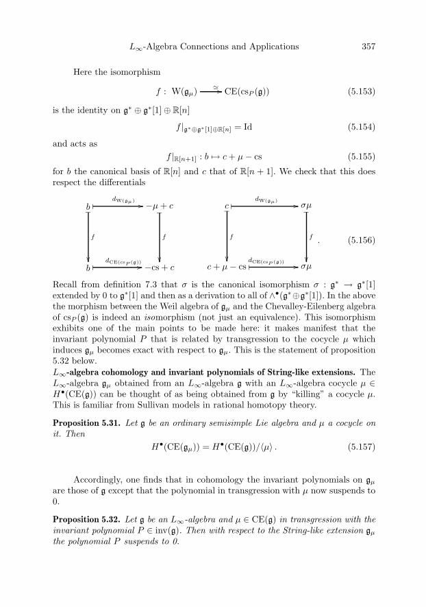
L∞-Algebra Connections and Applications 357
Here the isomorphism
f : W(gμ) � �� CE(csP (g)) (5.153)
is the identity on g∗ ⊕ g∗[1]⊕ R[n]
f |g∗⊕g∗[1]⊕R[n] = Id (5.154)
and acts asf |R[n+1] : b �→ c + μ− cs (5.155)
for b the canonical basis of R[n] and c that of R[n + 1]. We check that this doesrespect the differentials
b� dW(gμ) ��
�
f
��
−μ + c�
f
��b� dCE(csP (g)) �� −cs + c
c � dW(gμ) ���
f
��
σμ�
f
��c + μ− cs �dCE(csP (g)) �� σμ
. (5.156)
Recall from definition 7.3 that σ is the canonical isomorphism σ : g∗ → g∗[1]extended by 0 to g∗[1] and then as a derivation to all of ∧•(g∗⊕g∗[1]). In the abovethe morphism between the Weil algebra of gμ and the Chevalley-Eilenberg algebraof csP (g) is indeed an isomorphism (not just an equivalence). This isomorphismexhibits one of the main points to be made here: it makes manifest that theinvariant polynomial P that is related by transgression to the cocycle μ whichinduces gμ becomes exact with respect to gμ. This is the statement of proposition5.32 below.L∞-algebra cohomology and invariant polynomials of String-like extensions. TheL∞-algebra gμ obtained from an L∞-algebra g with an L∞-algebra cocycle μ ∈H•(CE(g)) can be thought of as being obtained from g by “killing” a cocycle μ.This is familiar from Sullivan models in rational homotopy theory.
Proposition 5.31. Let g be an ordinary semisimple Lie algebra and μ a cocycle onit. Then
H•(CE(gμ)) = H•(CE(g))/〈μ〉 . (5.157)
Accordingly, one finds that in cohomology the invariant polynomials on gμ
are those of g except that the polynomial in transgression with μ now suspends to0.
Proposition 5.32. Let g be an L∞-algebra and μ ∈ CE(g) in transgression with theinvariant polynomial P ∈ inv(g). Then with respect to the String-like extension gμ
the polynomial P suspends to 0.
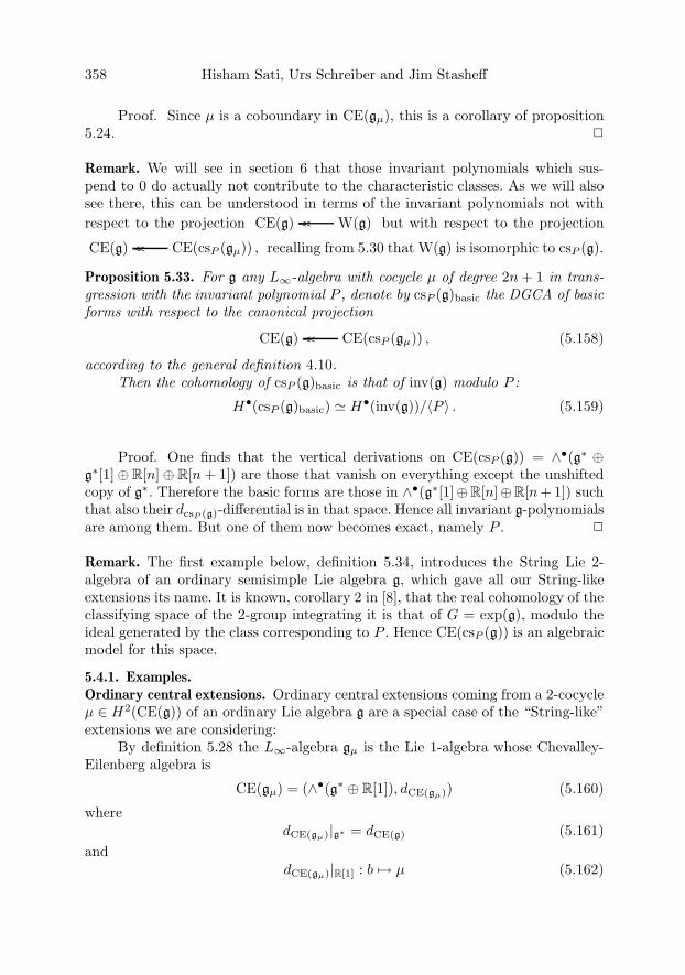
358 Hisham Sati, Urs Schreiber and Jim Stasheff
Proof. Since μ is a coboundary in CE(gμ), this is a corollary of proposition5.24. �
Remark. We will see in section 6 that those invariant polynomials which sus-pend to 0 do actually not contribute to the characteristic classes. As we will alsosee there, this can be understood in terms of the invariant polynomials not withrespect to the projection CE(g) W(g)���� but with respect to the projection
CE(g) CE(csP (gμ)) ,���� recalling from 5.30 that W(g) is isomorphic to csP (g).
Proposition 5.33. For g any L∞-algebra with cocycle μ of degree 2n + 1 in trans-gression with the invariant polynomial P , denote by csP (g)basic the DGCA of basicforms with respect to the canonical projection
CE(g) CE(csP (gμ)) ,���� (5.158)
according to the general definition 4.10.Then the cohomology of csP (g)basic is that of inv(g) modulo P :
H•(csP (g)basic) � H•(inv(g))/〈P 〉 . (5.159)
Proof. One finds that the vertical derivations on CE(csP (g)) = ∧•(g∗ ⊕g∗[1]⊕ R[n]⊕ R[n + 1]) are those that vanish on everything except the unshiftedcopy of g∗. Therefore the basic forms are those in ∧•(g∗[1]⊕R[n]⊕R[n+ 1]) suchthat also their dcsP (g)-differential is in that space. Hence all invariant g-polynomialsare among them. But one of them now becomes exact, namely P . �
Remark. The first example below, definition 5.34, introduces the String Lie 2-algebra of an ordinary semisimple Lie algebra g, which gave all our String-likeextensions its name. It is known, corollary 2 in [8], that the real cohomology of theclassifying space of the 2-group integrating it is that of G = exp(g), modulo theideal generated by the class corresponding to P . Hence CE(csP (g)) is an algebraicmodel for this space.
5.4.1. Examples.Ordinary central extensions. Ordinary central extensions coming from a 2-cocycleμ ∈ H2(CE(g)) of an ordinary Lie algebra g are a special case of the “String-like”extensions we are considering:
By definition 5.28 the L∞-algebra gμ is the Lie 1-algebra whose Chevalley-Eilenberg algebra is
CE(gμ) = (∧•(g∗ ⊕ R[1]), dCE(gμ)) (5.160)
wheredCE(gμ)|g∗ = dCE(g) (5.161)
anddCE(gμ)|R[1] : b �→ μ (5.162)
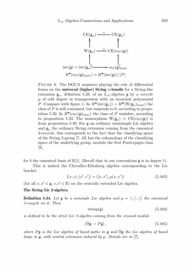
L∞-Algebra Connections and Applications 359
CE(gμ) = CE(gμ)
W(gμ) �
����
CE(csP (g))
����
inv(g) = inv(gμ) � � ��� �
��
csP (g)basic
� �
��
H•(csP (g)basic) � H•(inv(g))/〈P 〉
Figure 8. The DGCA sequence playing the role of differentialforms on the universal (higher) String n-bundle for a String-likeextension gμ, definition 5.28, of an L∞-algebra g by a cocycleμ of odd degree in transgression with an invariant polynomialP . Compare with figure 1. In H•(inv(gμ)) = H•(W(gμ)basic) theclass of P is still contained, but suspends to 0, according to propo-sition 5.32. In H•(csP (g)basic) the class of P vanishes, accordingto proposition 5.33. The isomorphism W(gμ) � CE(csP (g)) isfrom proposition 5.30. For g an ordinary semisimple Lie algebraand gμ the ordinary String extension coming from the canonical3-cocycle, this corresponds to the fact that the classifying spaceof the String 2-group [7, 43] has the cohomology of the classifyingspace of the underlying group, modulo the first Pontrajagin class[8].
for b the canonical basis of R[1]. (Recall that in our conventions g is in degree 1).This is indeed the Chevalley-Eilenberg algebra corresponding to the Lie
bracket[(x, c), (x′, c′)] = ([x, x′], μ(x, x′)) (5.163)
(for all x, x′ ∈ g, c, c′ ∈ R) on the centrally extended Lie algebra.
The String Lie 2-algebra.
Definition 5.34. Let g be a semisiple Lie algebra and μ = 〈·, [·, ·]〉 the canonical3-cocycle on it. Then
string(g) (5.164)
is defined to be the strict Lie 2-algebra coming from the crossed module
(Ωg → Pg) , (5.165)
where Pg is the Lie algebra of based paths in g and Ωg the Lie algebra of basedloops in g, with central extension induced by μ. Details are in [7].

360 Hisham Sati, Urs Schreiber and Jim Stasheff
Proposition 5.35 ([7]). The Lie 2-algebra gμ obtained from g and μ as in definition5.28 is equivalent to the strict string Lie 2-algebra
gμ � string(g) . (5.166)
This means there are morphisms gμ → string(g) and string(g) → gμ whosecomposite is the identity only up to homotopy
gμ ��
Id
� string(g) �� gμ
=
string(g) ��
Id
� gμ �� string(g)
η
(5.167)
We call gμ the skeletal and string(g) the strict version of the String Lie2-algebra.The Fivebrane Lie 6-algebra.
Definition 5.36. Let g = so(n) and μ the canonical 7-cocycle on it. Then
fivebrane(g) (5.168)
is defined to be the strict Lie 7-algebra which is equivalent to gμ
gμ � fivebrane(g) . (5.169)
A Lie n-algebra is strict if it corresponds to a differential graded Lie algebraon a vector space in degree 1 to n. (Recall our grading conventions from 5.1.) Thestrict Lie n-algebras corresponding to certain weak Lie n-algebras can be foundby first integrating to strict Lie n-groups and then differentiating the result again.This shall not concern us here, but discussion of this point can be found in [71]and [70].The BF-theory Lie 3-algebra.
Definition 5.37. For g any ordinary Lie algebra with bilinear invariant symmetricform 〈·, ·〉 ∈ inv(g) in transgression with the 3-cocycle μ, and for h
t→ g a strictLie 2-algebra based on g, denote by
μ := dCE(h
t→g)μ (5.170)
the corresponding exact 4-cocycle on (h t→ g) discussed in 5.3.1. Then we call theString-like extended Lie 3-algebra
bf(h t→ g) := (h t→ g)μ (5.171)
the corresponding BF-theory Lie 3-algebra.
The terminology here will become clear once we describe in 7.3.1 and 8.1.1how the BF-theory action functional discussed in 5.6.1 arises as the parallel 4-transport given by the b3u(1)-4-bundle which arises as the obstruction to lifting(h t→ g)-2-descent objects to bf(h t→ g)-3-descent objects.
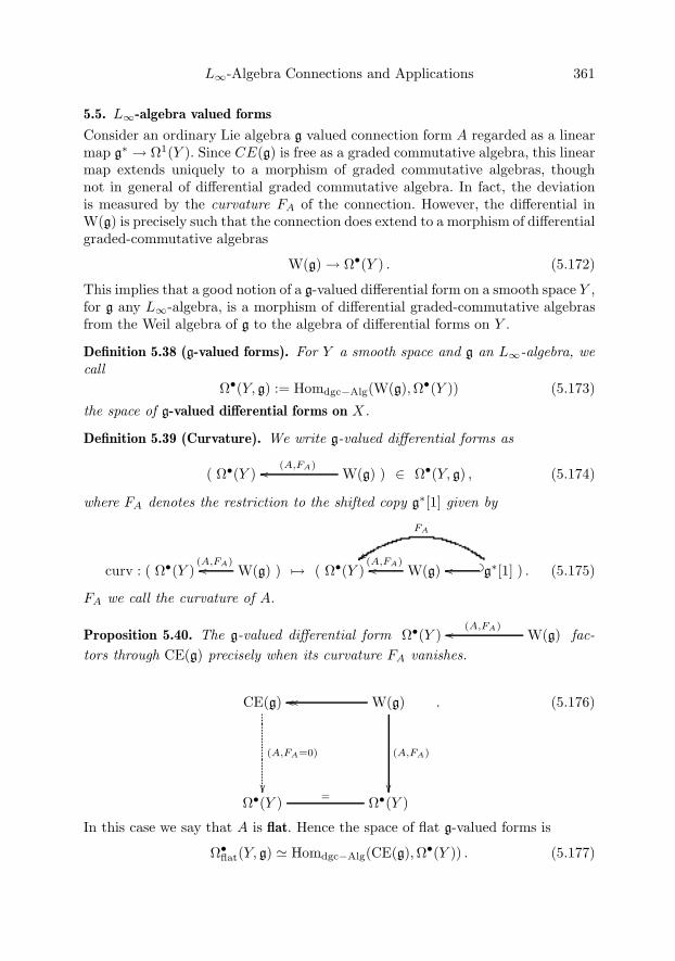
L∞-Algebra Connections and Applications 361
5.5. L∞-algebra valued forms
Consider an ordinary Lie algebra g valued connection form A regarded as a linearmap g∗ → Ω1(Y ). Since CE(g) is free as a graded commutative algebra, this linearmap extends uniquely to a morphism of graded commutative algebras, thoughnot in general of differential graded commutative algebra. In fact, the deviationis measured by the curvature FA of the connection. However, the differential inW(g) is precisely such that the connection does extend to a morphism of differentialgraded-commutative algebras
W(g) → Ω•(Y ) . (5.172)
This implies that a good notion of a g-valued differential form on a smooth space Y ,for g any L∞-algebra, is a morphism of differential graded-commutative algebrasfrom the Weil algebra of g to the algebra of differential forms on Y .
Definition 5.38 (g-valued forms). For Y a smooth space and g an L∞-algebra, wecall
Ω•(Y, g) := Homdgc−Alg(W(g),Ω•(Y )) (5.173)
the space of g-valued differential forms on X.
Definition 5.39 (Curvature). We write g-valued differential forms as
( Ω•(Y ) W(g)(A,FA)�� ) ∈ Ω•(Y, g) , (5.174)
where FA denotes the restriction to the shifted copy g∗[1] given by
curv : ( Ω•(Y ) W(g)(A,FA)�� ) �→ ( Ω•(Y ) W(g)
(A,FA)�� g∗[1]� ���
FA
��) . (5.175)
FA we call the curvature of A.
Proposition 5.40. The g-valued differential form ٕ(Y ) W(g)(A,FA)�� fac-
tors through CE(g) precisely when its curvature FA vanishes.
CE(g)
(A,FA=0)
��
W(g)����
(A,FA)
��ٕ(Y ) = ٕ(Y )
. (5.176)
In this case we say that A is flat. Hence the space of flat g-valued forms is
Ω•flat(Y, g) � Homdgc−Alg(CE(g),Ω•(Y )) . (5.177)

362 Hisham Sati, Urs Schreiber and Jim Stasheff
Bianchi identity. Recall from 5.1 that the Weil algebra W(g) of an L∞-algebra gis the same as the Chevalley-Eilenberg algebra CE(inn(g)) of the L∞-algebra ofinner derivation of g. It follows that g-valued differential forms on Y are the sameas flat inn(g)-valued differential forms on Y :
Ω•(Y, g) = Ω•flat(inn(g)) . (5.178)
By the above definition of curvature, this says that the curvature FA of a g-valued connection (A,FA) is itself a flat inn(g)-valued connection. This is thegeneralization of the ordinary Bianchi identity to L∞-algebra valued forms.
Definition 5.41. Two g-valued forms A,A′ ∈ Ω•(Y, g) are called (gauge) equivalentprecisely if they are related by a vertical concordance, i.e. by a concordance, suchthat the corresponding derivation ρ from proposition 5.14 is vertical, in the senseof definition 4.9.
5.5.1. Examples.1. Ordinary Lie-algebra valued 1-forms. We have already mentioned ordinary Liealgebra valued 1-forms in this general context in 2.1.3.2. Forms with values in shifted bn−1u(1). A bn−1u(1)-valued form is nothing butan ordinary n-form A ∈ Ωn(Y ):
Ω•(bn−1u(1), Y ) � Ωn(Y ) . (5.179)
A flat bn−1u(1)-valued form is precisely a closed n-form.
CE(bn−1u(1))
(A)
dA=0
��
���� W(bn−1u(1))
(A,FA)
A=dA
��ٕ(Y ) = �� ٕ(Y )
3. Crossed module valued forms. Let g(2) = (h t→ g) be a strict Lie 2-algebracoming from a crossed module. Then a g(2)-valued form is an ordinary g-valued1-form A and an ordinary h-valued 2-form B. The corresponding curvature isan ordinary g-valued 2-form β = FA + t(B) and an ordinary h-valued 3-formH = dAB. This is denoted by the right vertical arrow in the following diagram.
CE(h t→ g)
(A,B)
FA+t(B)=0
��
W(h t→ g)����
(A,B,β,H)
β=FA+t(B)H=dAB
��ٕ(Y ) = ٕ(Y )
. (5.180)
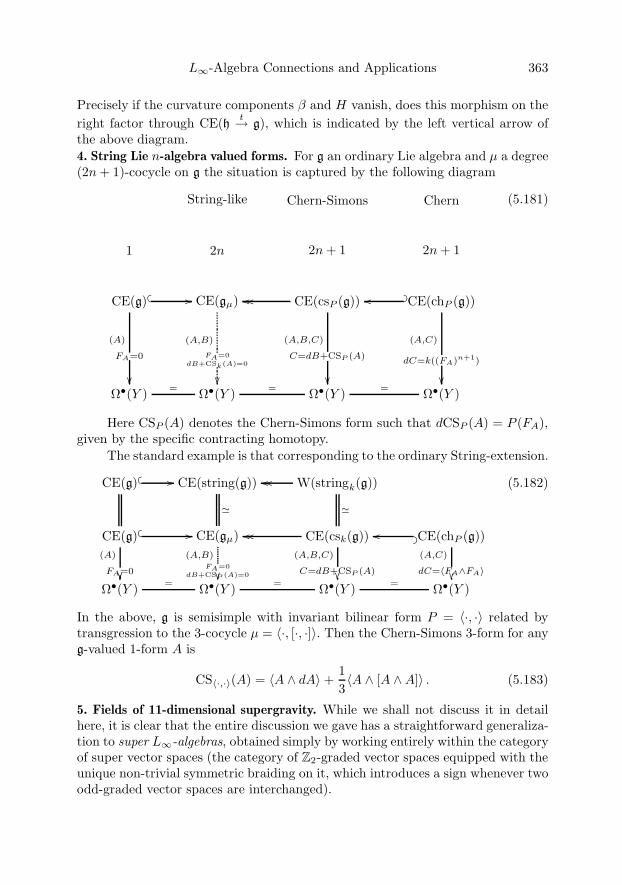
L∞-Algebra Connections and Applications 363
Precisely if the curvature components β and H vanish, does this morphism on theright factor through CE(h t→ g), which is indicated by the left vertical arrow ofthe above diagram.4. String Lie n-algebra valued forms. For g an ordinary Lie algebra and μ a degree(2n + 1)-cocycle on g the situation is captured by the following diagram
String-like Chern-Simons Chern
1 2n 2n + 1 2n + 1
CE(g) CE(gμ)��� � ���� CE(csP (g)) �� � �CE(chP (g))
ٕ(Y ) =��
(A)
FA=0
ٕ(Y ) =��
(A,B)
FA=0dB+CSk(A)=0
ٕ(Y ) =��
(A,B,C)
C=dB+CSP (A)
ٕ(Y )��
(A,C)
dC=k((FA)n+1)
(5.181)
Here CSP (A) denotes the Chern-Simons form such that dCSP (A) = P (FA),given by the specific contracting homotopy.
The standard example is that corresponding to the ordinary String-extension.
CE(g) CE(string(g))��� � ����
�
W(stringk(g))
CE(g) CE(gμ)��� � ���� CE(csk(g))
�
�� �� CE(chP (g))
ٕ(Y ) =��
(A)
FA=0
ٕ(Y ) =��
(A,B)FA=0
dB+CSP (A)=0
ٕ(Y ) =��
(A,B,C)
C=dB+CSP (A)
ٕ(Y )��
(A,C)
dC=〈FA∧FA〉
(5.182)
In the above, g is semisimple with invariant bilinear form P = 〈·, ·〉 related bytransgression to the 3-cocycle μ = 〈·, [·, ·]〉. Then the Chern-Simons 3-form for anyg-valued 1-form A is
CS〈·,·〉(A) = 〈A ∧ dA〉 +13〈A ∧ [A ∧A]〉 . (5.183)
5. Fields of 11-dimensional supergravity. While we shall not discuss it in detailhere, it is clear that the entire discussion we gave has a straightforward generaliza-tion to super L∞-algebras, obtained simply by working entirely within the categoryof super vector spaces (the category of Z2-graded vector spaces equipped with theunique non-trivial symmetric braiding on it, which introduces a sign whenever twoodd-graded vector spaces are interchanged).

364 Hisham Sati, Urs Schreiber and Jim Stasheff
A glance at the definitions shows that, up to mere differences in terminology,the theory of “FDA”s (“free differential algebras”) considered in [4, 24] is nothingbut that of what we call qDGCAs here: quasi-free differential graded commutativealgebras.
Using that and the interpretation of qDGCAs in terms of L∞-algebras, onecan translate everything said in [4, 24] into our language here to obtain the fol-lowing statement:
The field content of 11-dimensional supergravity is nothing but a g-valuedform, for
g = sugra(10, 1) (5.184)
the Lie 3-algebra which is the String-like extension
0 → b2u(1) → sugra(10, 1) → siso(10, 1) → 0 (5.185)
of the super-Poincare Lie algebra in 10+1 dimensions, coming from a certain 4-cocycle on that.
CE(sugra(10, 1))
(flat connection,parallel gravitino,
vanishing supertorsion)
��
W(sugra(10, 1))����
(graviton g,gravitino Ψ,3-form C3)
��ٕ(Y ) = ٕ(Y )
(5.186)
While we shall not further pursue this here, this implies the following twointeresting issues.
• It is known in string theory [28] that the supergravity 3-form in fact consists ofthree parts: two Chern-Simons parts for an e8 and for a so(10, 1)-connection,as well as a further fermionic part, coming precisely from the 4-cocycle thatgoverns sugra(10, 1). As we discuss in 7 and 8, the two Chern-Simons com-ponents can be understood in terms of certain Lie 3-algebra connectionscoming from the Chern-Simons Lie 3-algebra csP (g) from definition 5.28. Ithence seems that there should be a Lie n-algebra which nicely unifies csP (e8),csP (so(10, 1)8) and sugra(10, 1). This remains to be discussed.
• The discussion in section 6 shows how to obtain from g-valued forms globallydefined connections on possibly nontrivial g-n-bundles. Applied tosugra(10, 1) this should yield a global description of the supergravity fieldcontent, which extends the local field content considered in [4, 24] in the waya connection in a possibly nontrivial Yang-Mills bundle generalizes a Lie al-gebra valued 1-form. This should for instance allow to discuss supergravityinstanton solutions.

L∞-Algebra Connections and Applications 365
5.6. L∞-algebra characteristic forms
Definition 5.42. For g any L∞ algebra and
ٕ(Y ) W(g)(A,FA)�� (5.187)
any g-valued differential form, we call the composite
ٕ(Y ) W(g)(A,FA)�� inv(g)� ���
{P (FA)}
��(5.188)
the collection of invariant forms of the g-valued form A. We call the de Rhamclasses [P (FA)] of the characteristic forms arising as the image of closed invariantpolynomials
ٕ(Y ) W(g)(A,FA)�� inv(g)� ���
{Pi(FA)}
��
H•dR(Y ) H•(inv(g))
{[P (FA)]}��
(5.189)
the collection of characteristic classes of the g-valued form A.
Recall from section 5.3 that for ordinary Lie algebras all invariant polynomialsare closed, while for general L∞-algebras it is only true that their dW(g)-differentialis horizontal. Notice that Y will play the role of a cover of some space X soon, andthat characteristic forms really live down on X . We will see shortly a constraintimposed which makes the characteristic forms descend down from the Y here tosuch an X .
Proposition 5.43. Under gauge transformations as in definition 5.41, characteristicclasses are invariant.
Proof. This follows from proposition 5.14: By that proposition, the derivativeof the concordance form A along the interval I = [0, 1] is a chain homotopy
d
dtA(P ) = [d, ιX ]P = dτ(P ) + ιX(dW(g)P ) . (5.190)
By definition of gauge-transformations, ιX is vertical. By definition of basic forms,P is both in the kernel of ιX as well as in the kernel of ιX ◦ d. Hence the righthand vanishes. �
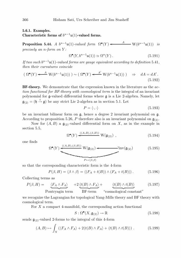
366 Hisham Sati, Urs Schreiber and Jim Stasheff
5.6.1. Examples.Characteristic forms of bn−1u(1)-valued forms.
Proposition 5.44. A bn−1u(1)-valued form Ω•(Y ) W(bn−1u(1))A�� isprecisely an n-form on Y :
Ω•(Y, bn−1u(1)) � Ωn(Y ) . (5.191)
If two such bn−1u(1)-valued forms are gauge equivalent according to definition 5.41,then their curvatures coincide
( Ω•(Y ) W(bn−1u(1))A�� ) ∼ ( Ω•(Y ) W(bn−1u(1))A′�� ) ⇒ dA = dA′ .
(5.192)
BF-theory. We demonstrate that the expression known in the literature as the ac-tion functional for BF-theory with cosmological term is the integral of an invariantpolynomial for g-valued differential forms where g is a Lie 2-algebra. Namely, letg(2) = (h t→ g) be any strict Lie 2-algebra as in section 5.1. Let
P = 〈·, ·〉 (5.193)
be an invariant bilinear form on g, hence a degree 2 invariant polynomial on g.According to proposition 5.26, P therefore also is an invariant polynomial on g(2).
Now for (A,B) a g(2)-valued differential form on X , as in the example insection 5.5,
Ω•(Y ) W(g(2))((A,B),(β,H))�� , (5.194)
one finds
Ω•(Y ) W(g(2))((A,B),(β,H))�� inv(g(2))� ���
P �→〈β,β〉
! (5.195)
so that the corresponding characteristic form is the 4-form
P (β,H) = 〈β ∧ β〉 = 〈(FA + t(B)) ∧ (FA + t(B))〉 . (5.196)
Collecting terms as
P (β,H) = 〈FA ∧ FA〉︸ ︷︷ ︸Pontryagin term
+2 〈t(B) ∧ FA〉︸ ︷︷ ︸BF-term
+ 〈t(B) ∧ t(B)〉︸ ︷︷ ︸“cosmological constant”
(5.197)
we recognize the Lagrangian for topological Yang-Mills theory and BF theory withcosmological term.
For X a compact 4-manifold, the corresponding action functional
S : Ω•(X, g(2)) → R (5.198)
sends g(2)-valued 2-forms to the integral of this 4-form
(A,B) �→∫
X
(〈FA ∧ FA〉+ 2〈t(B) ∧ FA〉+ 〈t(B) ∧ t(B)〉) . (5.199)

L∞-Algebra Connections and Applications 367
The first term here is usually not considered an intrinsic part of BF-theory, butits presence does not affect the critical points of S.
The critical points of S, i.e. the g(2)-valued differential forms on X that satisfythe equations of motion defined by the action S, are given by the equation
β := FA + t(B) = 0 . (5.200)
Notice that this impliesdAt(B) = 0 (5.201)
but does not constrain the full 3-curvature
H = dAB (5.202)
to vanish. In other words, the critical points of S are precisely the fake flat g(2)-valued forms which precisely integrate to strict parallel transport 2-functors [38,73, 9].
While the 4-form 〈β ∧ β〉 looks similar to the Pontrjagin 4-form 〈FA ∧ FA〉for an ordinary connection 1-form A, one striking difference is that 〈β ∧ β〉 is, ingeneral, not closed. Instead, according to equation (5.127), we have
d〈β ∧ β〉 = 2〈β ∧ t(H)〉 . (5.203)
Remark. Under the equivalence [7] of the skeletal String Lie 2-algebra to itsstrict version, recalled in proposition 5.35, the characteristic forms for strict Lie2-algebras apply also to one of our central objects of interest here, the String 2-connections. But a little care needs to be exercised here, because the strict versionof the String Lie 2-algebra is no longer finite dimensional.Remark. Our interpretation above of BF-theory as a gauge theory for Lie 2-algebras is not unrelated to, but different from the one considered in [38, 39].There only the Lie 2-algebra coming from the infinitesimal crossed module (|g| 0→g
ad→ der(g)) (for g any ordinary Lie algebra and |g| its underlying vector space,regarded as an abelian Lie algebra) is considered, and the action is restricted tothe term
∫〈FA∧B〉. We can regard the above discussion as a generalization of this
approach to arbitrary Lie 2-algebras. Standard BF-theory (with “cosmological”term) is reproduced with the above Lagrangian by using the Lie 2-algebra inn(g)corresponding to the infinitesimal crossed module (g Id→ g
ad→ der(g)) discussed insection 5.1.1.
6. L∞-algebra Cartan-Ehresmann connections
We will now combine all of the above ingredients to produce a definition of g-valued connections. As we shall explain, the construction we give may be thoughtof as a generalization of the notion of a Cartan-Ehresmann connection, which isgiven by a Lie algebra-valued 1-form on the total space of a bundle over base spacesatisfying two conditions:

368 Hisham Sati, Urs Schreiber and Jim Stasheff
• first Cartan-Ehresmann condition: on the fibers the connection form restrictsto a flat canonical form
• second Cartan-Ehresmann condition: under vertical flows the connectionstransforms nicely, in such a way that its characteristic forms descend downto base space.We will essentially interpret these two conditions as a pullback of the universal
g-bundle, in its DGC-algebraic incarnation as given in equation (5.94).The definition we give can also be seen as the Lie algebraic image of a similar
construction involving locally trivializable transport n-functors [9, 74], but thisshall not be further discussed here.
6.1. g-bundle descent data
Definition 6.1 (g-bundle descent data). Given a Lie n-algebra g, a g-bundle descentobject on X is a pair (Y,Avert) consisting of a choice of surjective submersionπ : Y → X with connected fibers (this condition will be dropped when we extendto g-connection descent objects in (6.2) together with a morphism of dg-algebras
Ω•vert(Y ) CE(g)
Avert�� . (6.1)
Two such descent objects are taken to be equivalent
( Ω•vert(Y ) CE(g)
Avert�� ) ∼ ( Ω•vert(Y
′) CE(g)A′
vert�� ) (6.2)
precisely if their pullbacks π∗1Avert and π∗
2A′vert to the common refinement
Y ×X Y ′ π1 ��
π2
��
Y
π
��Y ′ π′
�� X
(6.3)
are concordant in the sense of definition 5.13.
Thus two such descent objects Avert, A′vert on the same Y are equivalent if
there is η∗vert such that
Ω•vert(Y ) Ω•
vert(Y × I)s∗��t∗�� CE(g)
η∗vert��
Avert
!"
A′vert
��. (6.4)
Recall from the discussion in section 2.2.1 that the surjective submersionshere play the role of open covers of X .
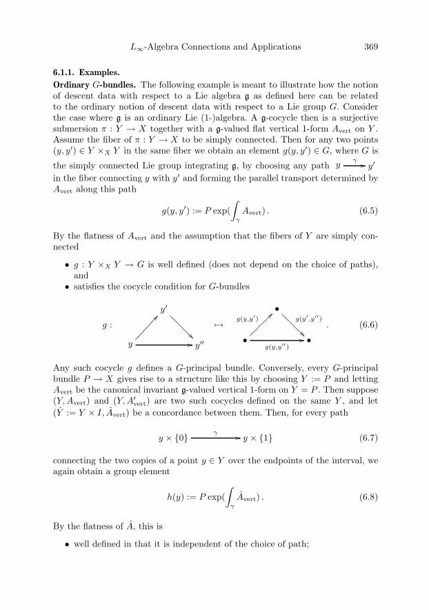
L∞-Algebra Connections and Applications 369
6.1.1. Examples.
Ordinary G-bundles. The following example is meant to illustrate how the notionof descent data with respect to a Lie algebra g as defined here can be relatedto the ordinary notion of descent data with respect to a Lie group G. Considerthe case where g is an ordinary Lie (1-)algebra. A g-cocycle then is a surjectivesubmersion π : Y → X together with a g-valued flat vertical 1-form Avert on Y .Assume the fiber of π : Y → X to be simply connected. Then for any two points(y, y′) ∈ Y ×X Y in the same fiber we obtain an element g(y, y′) ∈ G, where G is
the simply connected Lie group integrating g, by choosing any path yγ �� y′
in the fiber connecting y with y′ and forming the parallel transport determined byAvert along this path
g(y, y′) := P exp(∫
γ
Avert) . (6.5)
By the flatness of Avert and the assumption that the fibers of Y are simply con-nected
• g : Y ×X Y → G is well defined (does not depend on the choice of paths),and
• satisfies the cocycle condition for G-bundles
g :
y′
"#���
����
y ��
#$��������y′′
�→•
g(y′,y′′)
"#���
����
•g(y,y′′)
��
g(y,y′)$%������� •
. (6.6)
Any such cocycle g defines a G-principal bundle. Conversely, every G-principalbundle P → X gives rise to a structure like this by choosing Y := P and lettingAvert be the canonical invariant g-valued vertical 1-form on Y = P . Then suppose(Y,Avert) and (Y,A′
vert) are two such cocycles defined on the same Y , and let(Y := Y × I, Avert) be a concordance between them. Then, for every path
y × {0} γ �� y × {1} (6.7)
connecting the two copies of a point y ∈ Y over the endpoints of the interval, weagain obtain a group element
h(y) := P exp(∫
γ
Avert) . (6.8)
By the flatness of A, this is
• well defined in that it is independent of the choice of path;
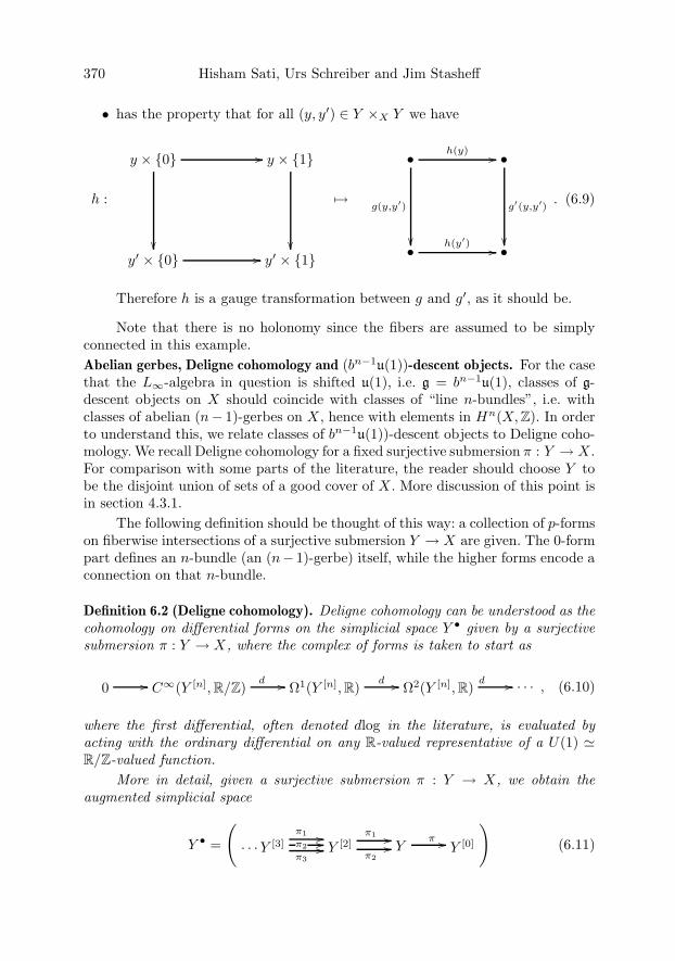
370 Hisham Sati, Urs Schreiber and Jim Stasheff
• has the property that for all (y, y′) ∈ Y ×X Y we have
h :
y × {0}
��
�� y × {1}
��y′ × {0} �� y′ × {1}
�→
•
g(y,y′)
��
h(y) �� •
g′(y,y′)
��• h(y′) �� •
. (6.9)
Therefore h is a gauge transformation between g and g′, as it should be.
Note that there is no holonomy since the fibers are assumed to be simplyconnected in this example.Abelian gerbes, Deligne cohomology and (bn−1u(1))-descent objects. For the casethat the L∞-algebra in question is shifted u(1), i.e. g = bn−1u(1), classes of g-descent objects on X should coincide with classes of “line n-bundles”, i.e. withclasses of abelian (n− 1)-gerbes on X , hence with elements in Hn(X,Z). In orderto understand this, we relate classes of bn−1u(1))-descent objects to Deligne coho-mology. We recall Deligne cohomology for a fixed surjective submersion π : Y → X .For comparison with some parts of the literature, the reader should choose Y tobe the disjoint union of sets of a good cover of X . More discussion of this point isin section 4.3.1.
The following definition should be thought of this way: a collection of p-formson fiberwise intersections of a surjective submersion Y → X are given. The 0-formpart defines an n-bundle (an (n− 1)-gerbe) itself, while the higher forms encode aconnection on that n-bundle.
Definition 6.2 (Deligne cohomology). Deligne cohomology can be understood as thecohomology on differential forms on the simplicial space Y • given by a surjectivesubmersion π : Y → X, where the complex of forms is taken to start as
0 �� C∞(Y [n],R/Z)d �� Ω1(Y [n],R)
d �� Ω2(Y [n],R)d �� · · · , (6.10)
where the first differential, often denoted dlog in the literature, is evaluated byacting with the ordinary differential on any R-valued representative of a U(1) �R/Z-valued function.
More in detail, given a surjective submersion π : Y → X, we obtain theaugmented simplicial space
Y • =
(· · ·Y [3]
π1 ��π2 ��π3
�� Y [2]π1 ��π2
�� Yπ �� Y [0]
)(6.11)
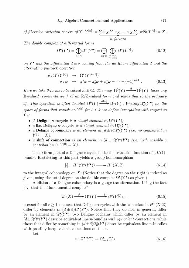
L∞-Algebra Connections and Applications 371
of fiberwise cartesian powers of Y , Y [n] := Y ×X Y ×X · · · ×X Y︸ ︷︷ ︸n factors
, with Y [0] := X.
The double complex of differential forms
Ω•(Y •) =⊕n∈N
Ωn(Y •) =⊕n∈N
⊕r,s∈N
r+s=n
Ωr(Y [s]) (6.12)
on Y • has the differential d ± δ coming from the de Rham differential d and thealternating pullback operation
δ : Ωr(Y [s]) → Ωr(Y [s+1])δ : ω �→ π∗
1ω − π∗2ω + π∗
3ω + · · · − (−1)s+1 . (6.13)
Here we take 0-forms to be valued in R/Z. The map Ω0(Y ) d �� Ω1(Y ) takes anyR-valued representative f of an R/Z-valued form and sends that to the ordinary
df . This operation is often denoted Ω0(Y )dlog �� Ω1(Y ) . Writing Ω•
k(Y •) for the
space of forms that vanish on Y [l] for l < k we define (everything with respect toY ):• A Deligne n-cocycle is a closed element in Ωn(Y •);• a flat Deligne n-cocycle is a closed element in Ωn
1 (Y •);• a Deligne coboundary is an element in (d± δ)Ω•
1(Y •) (i.e. no component inY [0] = X);
• a shift of connection is an element in (d ± δ)Ω•(Y •) (i.e. with possibly acontribution in Y [0] = X).
The 0-form part of a Deligne cocycle is like the transition function of a U(1)-bundle. Restricting to this part yields a group homomorphism
[·] : Hn(Ω•(Y •)) �� �� Hn(X,Z) (6.14)
to the integral cohomology on X . (Notice that the degree on the right is indeed asgiven, using the total degree on the double complex Ω•(Y •) as given.)
Addition of a Deligne coboundary is a gauge transformation. Using the fact[62] that the “fundamental complex”
Ωr(X) δ �� Ωr(Y ) δ �� Ωr(Y [2]) · · · (6.15)
is exact for all r ≥ 1, one sees that Deligne cocycles with the same class in Hn(X,Z)differ by elements in (d ± δ)Ω•(Y •). Notice that they do not, in general, differby an element in Ω•
1(Y •): two Deligne cochains which differ by an element in(d±δ)Ω•
1(Y•) describe equivalent line n-bundles with equivalent connections, while
those that differ by something in (d± δ)Ω•0(Y
•) describe equivalent line n-bundleswith possibly inequivalent connections on them.
Letv : Ω•(Y •) → Ω•
vert(Y ) (6.16)
372 Hisham Sati, Urs Schreiber and Jim Stasheff
be the map which sends each Deligne n-cochain a with respect to Y to the verticalpart of its (n− 1)-form on Y [1]
ν : a �→ a|Ωn−1vert (Y [1]) . (6.17)
(Recall the definition 4.11 of Ω•vert(Y ).) Then we have
Proposition 6.3. If two Deligne n-cocycles a and b over Y have the same class inHn(X,Z), then the classes of ν(a) and ν(b) coincide.
Proof. As mentioned above, a and b have the same class in Hn(X,Z) if andonly if they differ by an element in (d± δ)(Ω•(Y •)). This means that on Y [1] theydiffer by an element of the form
dα + δβ = dα + π∗β . (6.18)
Since π∗β is horizontal, this is exact in Ω•vert(Y [1]). �
Proposition 6.4. If the (n − 1)-form parts B,B′ ∈ Ωn−1(Y ) of two Deligne n-cocycles differ by a d± δ-exact part, then the two Deligne cocycles have the sameclass in Hn(X,Z).
Proof. If the surjective submersion is not yet contractible, we pull every-thing back to a contractible refinement, as described in section 4.3.1. So assumewithout restriction of generality that all Y [n] are contractible. This implies thatH•
deRham(Y [n]) = H0(Y [n]), which is a vector space spanned by the connectedcomponents of Y [n]. Now assume
B −B′ = dβ + δα (6.19)
on Y . We can immediately see that this implies that the real classes in Hn(X,R)coincide: the Deligne cocycle property says
d(B −B′) = δ(H −H ′) (6.20)
hence, by the exactness of the de Rham complex we have now,
δ(H −H ′) = δ(dα) (6.21)
and by the exactness of δ we get [H ] = [H ′].To see that also the integral classes coincide we use induction over k in Y [k].
For instance on Y [2] we have
δ(B −B′) = d(A−A′) (6.22)
and henceδdβ = d(A−A′) . (6.23)
Now using again the exactness of the de Rham differential d this implies
A−A′ = δβ + dγ . (6.24)
This way we work our way up to Y [n], where it then follows that the 0-form cocy-cles are coboundant, hence that they have the same class in Hn(X,Z). �

L∞-Algebra Connections and Applications 373
Proposition 6.5. bn−1u(1)-descent objects with respect to a given surjective sub-mersion Y are in bijection with closed vertical n-forms on Y :{
Ω•vert(Y ) CE(bn−1u(1))
Avert��}
↔ {Avert ∈ Ωnvert(Y ) , dAvert = 0} .
(6.25)Two such bn−1u(1) descent objects on Y are equivalent precisely if these formsrepresent the same cohomology class
(Avert ∼ A′vert) ⇔ [Avert] = [A′
vert] ∈ Hn(Ω•vert(Y )) . (6.26)
Proof. The first statement is a direct consequence of the definition of bn−1u(1)in section 5.1. The second statement follows from proposition 5.14 using the rea-soning as in proposition 5.43. �
Hence two Deligne cocycles with the same class in Hn(X,Z) indeed specifythe same class of bn−1u(1)-descent data.
6.2. Connections on g-bundles: the extension problem
It turns out that a useful way to conceive of the curvature on a non-flat g n-bundleis, essentially, as the (n + 1)-bundle with connection obstructing the existence ofa flat connection on the original g-bundle. This superficially trivial statement iscrucial for our way of coming to grips with non-flat higher bundles with connection.
Definition 6.6 (Descent object for g-connection). Given g-bundle descent object
Ω•vert(Y ) CE(g)
Avert�� (6.27)
as above, a g-connection on it is a completion of this morphism to a diagram
Ω•vert(Y ) CE(g)
Avert��
Ω•(Y )
i∗
����
W (g)
����
(A,FA)��
ٕ(X)��
π∗
��
inv(g)��
��
{Ki}��
. (6.28)
As before, two g-connection descent objects are taken to be equivalent, if theirpullbacks to a common refinement are concordant.
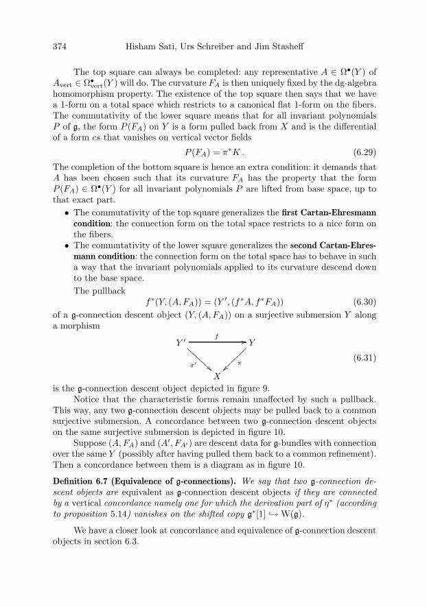
374 Hisham Sati, Urs Schreiber and Jim Stasheff
The top square can always be completed: any representative A ∈ Ω•(Y ) ofAvert ∈ Ω•
vert(Y ) will do. The curvature FA is then uniquely fixed by the dg-algebrahomomorphism property. The existence of the top square then says that we havea 1-form on a total space which restricts to a canonical flat 1-form on the fibers.The commutativity of the lower square means that for all invariant polynomialsP of g, the form P (FA) on Y is a form pulled back from X and is the differentialof a form cs that vanishes on vertical vector fields
P (FA) = π∗K . (6.29)
The completion of the bottom square is hence an extra condition: it demands thatA has been chosen such that its curvature FA has the property that the formP (FA) ∈ Ω•(Y ) for all invariant polynomials P are lifted from base space, up tothat exact part.• The commutativity of the top square generalizes the first Cartan-Ehresmann
condition: the connection form on the total space restricts to a nice form onthe fibers.
• The commutativity of the lower square generalizes the second Cartan-Ehres-mann condition: the connection form on the total space has to behave in sucha way that the invariant polynomials applied to its curvature descend downto the base space.The pullback
f∗(Y, (A,FA)) = (Y ′, (f∗A, f∗FA)) (6.30)of a g-connection descent object (Y, (A,FA)) on a surjective submersion Y alonga morphism
Y ′
π′���
����
���
f �� Y
π��
X
(6.31)
is the g-connection descent object depicted in figure 9.Notice that the characteristic forms remain unaffected by such a pullback.
This way, any two g-connection descent objects may be pulled back to a commonsurjective submersion. A concordance between two g-connection descent objectson the same surjective submersion is depicted in figure 10.
Suppose (A,FA) and (A′, FA′) are descent data for g-bundles with connectionover the same Y (possibly after having pulled them back to a common refinement).Then a concordance between them is a diagram as in figure 10.
Definition 6.7 (Equivalence of g-connections). We say that two g-connection de-scent objects are equivalent as g-connection descent objects if they are connectedby a vertical concordance namely one for which the derivation part of η∗ (accordingto proposition 5.14) vanishes on the shifted copy g∗[1] ↪→ W(g).
We have a closer look at concordance and equivalence of g-connection descentobjects in section 6.3.
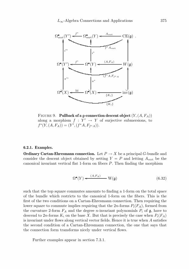
L∞-Algebra Connections and Applications 375
Ω•vert(Y
′) Ω•vert(Y )
f∗�� CE(g)
Avert��
f∗Avert
%&
Ω•(Y ′)
i′∗
����
Ω•(Y )f∗
��
i∗
����
W (g)
����
(A,FA)��
(f∗A,Ff∗A
%&
ٕ(X)��
π′∗
��
ٕ(X)Id����
π∗
��
inv(g)��
��
{Ki}��
{Ki}
%&
.
Figure 9. Pullback of a g-connection descent object (Y, (A,FA))along a morphism f : Y ′ → Y of surjective submersions, tof∗(Y, (A,FA)) = (Y ′, (f∗A,Ff∗A)).
6.2.1. Examples.
Ordinary Cartan-Ehresmann connection. Let P → X be a principal G-bundle andconsider the descent object obtained by setting Y = P and letting Avert be thecanonical invariant vertical flat 1-form on fibers P . Then finding the morphism
ٕ(Y ) W(g)(A,FA)�� (6.32)
such that the top square commutes amounts to finding a 1-form on the total spaceof the bundle which restricts to the canonical 1-form on the fibers. This is thefirst of the two conditions on a Cartan-Ehresmann connection. Then requiring thelower square to commute implies requiring that the 2n-forms Pi(FA), formed fromthe curvature 2-form FA and the degree n-invariant polynomials Pi of g, have todescend to 2n-forms Ki on the base X . But that is precisely the case when Pi(FA)is invariant under flows along vertical vector fields. Hence it is true when A satisfiesthe second condition of a Cartan-Ehresmann connection, the one that says thatthe connection form transforms nicely under vertical flows.
Further examples appear in section 7.3.1.

376 Hisham Sati, Urs Schreiber and Jim Stasheff
Ω•vert(Y ) Ω•
vert(Y )⊗ Ω•(I)s∗��t∗�� CE(g)
η∗vert��
Avert
&'
A′vert
!
Ω•(Y )
����
Ω•(Y )⊗ Ω•(I)
����
s∗��t∗�� W(g)
η∗��
����
(A,FA)
!"
(A′,FA′ )
!
ٕ(X)��
��
Ω•(X)⊗ Ω•(I)��
��
s∗��t∗�� inv(g)��
��
��
{Ki}
&'
{K′i}
!
Figure 10. Concordance between g-connection descent objects(Y, (A,FA)) and (Y, (A′, FA′)) defined on the same surjective sub-mersion π : Y → X . Concordance between descent objects not onthe same surjective submersion is reduced to this case by pullingboth back to a common refinement, as in figure 9.
6.3. Characteristic forms and characteristic classes
Definition 6.8. For any g-connection descent object (Y, (A,FA)) we say that in
Ω•vert(Y ) CE(g)
Avert��
Ω•(Y )
i∗����
W (g)
����
(A,FA)��
ٕ(X)��
π∗
��
inv(g)��
��
{Ki}��
H•dR(X) H•(inv(g)){[Ki]}
��
(6.33)
the {Ki} are the characteristic forms, while their de Rham classes [Ki] ∈H•
deRham(X) are the characteristic classes of (Y, (A,FA)).
Proposition 6.9. If two g-connection descent objects (Y, (A,FA)) and (Y ′, (A′, FA′))are related by a concordance as in figure 9 and figure 10 then they have the same
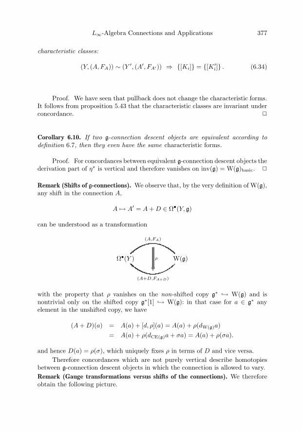
L∞-Algebra Connections and Applications 377
characteristic classes:
(Y, (A,FA)) ∼ (Y ′, (A′, FA′)) ⇒ {[Ki]} = {[K ′i]} . (6.34)
Proof. We have seen that pullback does not change the characteristic forms.It follows from proposition 5.43 that the characteristic classes are invariant underconcordance. �
Corollary 6.10. If two g-connection descent objects are equivalent according todefinition 6.7, then they even have the same characteristic forms.
Proof. For concordances between equivalent g-connection descent objects thederivation part of η∗ is vertical and therefore vanishes on inv(g) = W(g)basic. �
Remark (Shifts of g-connections). We observe that, by the very definition of W(g),any shift in the connection A,
A �→ A′ = A + D ∈ Ω•(Y, g)
can be understood as a transformation
Ω•(Y ) W(g)
(A,FA)
��
(A+D,FA+D)
��ρ
with the property that ρ vanishes on the non-shifted copy g∗ ↪→ W(g) and isnontrivial only on the shifted copy g∗[1] ↪→ W(g): in that case for a ∈ g∗ anyelement in the unshifted copy, we have
(A + D)(a) = A(a) + [d, ρ](a) = A(a) + ρ(dW(g)a)= A(a) + ρ(dCE(g)a + σa) = A(a) + ρ(σa).
and hence D(a) = ρ(σ), which uniquely fixes ρ in terms of D and vice versa.Therefore concordances which are not purely vertical describe homotopies
between g-connection descent objects in which the connection is allowed to vary.Remark (Gauge transformations versus shifts of the connections). We thereforeobtain the following picture.

378 Hisham Sati, Urs Schreiber and Jim Stasheff
• Vertical concordances relate gauge equivalent g-connections (compare defini-tion 5.41 of gauge transformations of g-valued forms)
(A,F
A)
and
(A′ ,F
A′ )
are
equi
vale
ntas
g-c
onne
ctio
ns
⇔ ∃
Ω•vert(Y ) Ω•
vert(Y )⊗ Ω•(I)s∗��t∗�� CE(g)
η∗vert��
Avert
&'
A′vert
!
Ω•(Y )
����
Ω•(Y )⊗ Ω•(I)
����
s∗��t∗�� W(g)
η∗��
����
(A,FA)
!"
(A′,FA′ )
!
ٕ(X)��
��
Ω•(X)⊗ Ω•(I)��
��
s∗��t∗�� inv(g)��
��
��(6.35)
• Non-vertical concordances relate g-connection descent objects whose underly-ing g-descent object – the underlying g-n-bundles – are equivalent, but whichpossibly differ in the choice of connection on these g-bundles:
(A′ ,F
A′ )
isob
tain
edfr
om(A
,FA)
bya
shift
ofg-c
onne
ctio
ns
⇔ ∃
Ω•vert(Y ) Ω•
vert(Y )⊗ Ω•(I)s∗��t∗�� CE(g)
η∗vert��
Ω•(Y )
����
Ω•(Y )⊗ Ω•(I)
����
s∗��t∗�� W(g)
η∗��
����
(A,FA)
!"
(A′,FA′ )
!
ٕ(X)��
��
Ω•(X)⊗ Ω•(I)��
��
s∗��t∗�� inv(g)��
��
��
{Ki}
&'
{K′i}
!
(6.36)
Remark. This in particular shows that for a given g-descent object
Ω•vert(Y ) CE(g)
Avert��
the corresponding characteristic classes obtained by choosing a connection (A,FA)does not depend on continuous variations of that choice of connection.
In the case of ordinary Lie (1-)algebras g it is well known that any twoconnections on the same bundle may be continuously connected by a path of
L∞-Algebra Connections and Applications 379
connections: the space of 1-connections is an affine space modeled on Ω1(X, g). Ifwe had an analogous statement for g-connections for higher L∞-algebras, we couldstrengthen the above statement.
6.3.1. Examples.
Ordinary characteristic classes of g-bundles. Let g be an ordinary Lie algebra and(Y, (A,FA)) be a g-descent object corresponding to an ordinary Cartan-Ehresmannconnection as in section 6.2.1. Using proposition 5.21 we know that inv(g) containsall the ordinary invariant polynomials P on g. Hence the characteristic classes[P (FA)] are precisely the standard characteristic classes (in de Rham cohomology)of the G-bundle with connection.
Characteristic classes of bn−1u(1)-bundles. For g = bn−1u(1) we have, accordingto proposition 5.25, inv(bn−1u(1)) = CE(bnu(1)) and hence a single degree n + 1characteristic class: the curvature itself.
This case we had already discussed in the context of Deligne cohomology insection 6.1.1. In particular, notice that in definition 6.2 we had already encounteredthe distinction between homotopies of L∞-algebra that are or are not pure gaugetransformations, in that they do or do not shift the connection: what is calleda Deligne coboundary in definition 6.2 corresponds to an equivalence of bn−1u-connection descent objects as in (6.35), while what is called a shift of connectionthere corresponds to a concordance that involves a shift as in (6.36).
6.4. Universal and generalized g-connections
We can generalize the discussion of g-bundles with connection on spaces X , by
• allowing all occurrences of the algebra of differential forms to be replacedwith more general differential graded algebras; this amounts to admittinggeneralized smooth spaces as in section 4.1;
• by allowing all Chevalley-Eilenberg and Weil algebras of L∞-algebras to bereplaced by DGCAs which may be nontrivial in degree 0. This amounts toallowing not just structure ∞-groups but also structure ∞-groupoids.
Definition 6.11 (Generalized g-connection descent objects). Given any L∞-algebrag, and given any DGCA A, we say a g-connection descent object for A is
• a surjection F Pi∗���� such that A � Pbasic;

380 Hisham Sati, Urs Schreiber and Jim Stasheff
• a choice of horizontal morphisms in the diagram
F CE(g)Avert��
P
i∗
����
W (g)
����
(A,FA)��
A��
��
inv(g)��
��
{Ki}��
; (6.37)
The notion of equivalence of these descent objects is as before.Horizontal forms. Given any algebra surjection
F
P
i∗
��
we know from definition 4.9 what the “vertical directions” on P are. After we havechosen a g-connection on P , we obtain also notion of horizontal elements in P :
Definition 6.12 (Horizontal elements). Given a g-connection (A,FA) on P , thealgebra of horizontal elements
horA(P ) ⊂ P
of P with respect to this connection are those elements not in the ideal generatedby the image of A.
Notice that horA(P ) is in general just a graded-commutative algebra, not adifferential algebra. Accordingly the inclusion horA(P ) ⊂ P is meant just as aninclusion of algebras.
6.4.1. Examples.The universal g-connection. The tautological example is actually of interest: forany L∞-algebra g, there is a canonical g-connection descent object on inv(g). Thiscomes from choosing
( F Pi∗���� ) := ( CE(g) W(g)i∗���� ) (6.38)
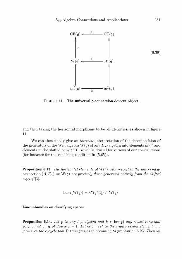
L∞-Algebra Connections and Applications 381
CE(g) CE(g)Id��
W(g)
i∗
����
W (g)
����
Id��
inv(g)��
��
inv(g)��
��
Id��
(6.39)
Figure 11. The universal g-connection descent object.
and then taking the horizontal morphisms to be all identities, as shown in figure11.
We can then finally give an intrinsic interpretation of the decomposition ofthe generators of the Weil algebra W(g) of any L∞-algebra into elements in g∗ andelements in the shifted copy g∗[1], which is crucial for various of our constructions(for instance for the vanishing condition in (5.65)).
Proposition 6.13. The horizontal elements of W(g) with respect to the universal g-connection (A,FA) on W(g) are precisely those generated entirely from the shiftedcopy g∗[1]:
horA(W(g)) = ∧•(g∗[1]) ⊂ W(g) .
Line n-bundles on classifying spaces.
Proposition 6.14. Let g be any L∞-algebra and P ∈ inv(g) any closed invariantpolynomial on g of degree n + 1. Let cs := τP be the transgression element andμ := i∗cs the cocycle that P transgresses to according to proposition 5.23. Then we

382 Hisham Sati, Urs Schreiber and Jim Stasheff
canonically obtain a bn−1u(1)-connection descent object in inv(g):
CE(g) CE(bn−1u(1))μ��
W(g)
i∗
����
W (bn−1u(1))
����
(cs,P )��
inv(g)��
��
inv(bnu(1)) = CE(bn−1u(1))��
��
P��
(6.40)
Remark. For instance for g an ordinary semisimple Lie algebra and μ its canonical3-cocylce, we obtain a descent object for a Lie 3-bundle which plays the role ofwhat is known as the canonical 2-gerbe on the classifying space BG of the simplyconnected group G integrating g [21]. From the above and using section 5.5.1 weread off that its connection 3-form is the canonical Chern-Simons 3-form. We willsee this again in 8.3.1, where we show that the 3-particle (the 2-brane) coupled tothe above g-connection descent object indeed reproduces Chern-Simons theory.
7. Higher string- and Chern-Simons n-bundles: the lifting problem
We discuss the general concept of weak cokernels of morphisms of L∞-algebras.Then we apply this to the special problem of lifts of differential g-cocycles throughString-like extensions.
7.1. Weak cokernels of L∞-morphisms
After introducing the notion of a mapping cone of qDGCAs, the main point hereis proposition 7.8, which establishes the existence of the weak inverse f−1 that wasmentioned in section 2.3. It will turn out to be that very weak inverse which picksup the information about the existence or non-existence of the lifts discussed insection 7.3. We can define the weak cokernel for normal L∞-subalgebras :
Definition 7.1 (Normal L∞-subalgebra). We say a Lie ∞-algebra h is a normalsub L∞-algebra of the L∞-algebra g if there is a morphism
CE(h) CE(g)t∗���� (7.1)
which the property that
• on g∗ it restricts to a surjective linear map h∗ g∗t∗1���� ;
• if a ∈ ker(t∗) then dCE(g)a ∈ ∧•(ker(t∗1)).

L∞-Algebra Connections and Applications 383
Proposition 7.2. For h and g ordinary Lie algebras, the above notion of normalsub L∞-algebra coincides with the standard notion of normal sub Lie algebras.
Proof. If a ∈ ker(t∗) then for any x, y ∈ g the condition says that(dCE(g)a)(x ∨ y) = −a(D[x ∨ y]) = −a([x, y]) vanishes when x or y are in theimage of t. But a([x, y]) vanishes when [x, y] is in the image of t. Hence the con-dition says that if at least one of x and y is in the image of t, then their bracket is. �
Definition 7.3 (Mapping cone of qDGCAs; Crossed module of normal sub L∞-al-
gebras). Let t : h ↪→ g be an inclusion of a normal sub L∞-algebra h into g. Themapping cone of t∗ is the qDGCA whose underlying graded algebra is
∧•(g∗ ⊕ h∗[1]) (7.2)
and whose differential dt is such that it acts on generators schematically as
dt =(
dg 0t∗ dh
). (7.3)
In more detail, dt∗ is defined as follows. We write σt∗ for the degree +1derivation on ∧•(g∗ ⊕ h∗[1]) which acts on g∗ as t∗ followed by a shift in degreeand which acts on h∗[1] as 0. Then, for any a ∈ g∗, we have
dta := dCE(g)a + σt∗(a) . (7.4)
anddtσt
∗(a) := −σt∗(dCE(g)a) = −dtdCE(g)a . (7.5)
Notice that the last equation
• defines dt on all of h∗[1] since t∗ is surjective;• is well defined in that it agrees for a and a′ if t∗(a) = t∗(a′), since t is normal.
Proposition 7.4. The differential dt defined this way indeed satisfies (dt)2 = 0.
Proof. For a ∈ g∗ we have
dtdta = dt(dCE(g)a + σt∗(a)) = σt∗(dCE(g)a)− σt∗(dCE(g)a) = 0 . (7.6)
Hence (dt)2 vanishes on ∧•(g∗). Since
dtdtσt∗(a) = −dtdtdCE(g)a (7.7)
and since dCE(g)a ∈ ∧•(g∗) this implies (dt)2 = 0. �
We write CE(ht↪→ g) := (∧•(g∗ ⊕ h∗[1]), dt) for the resulting qDGCA and
(ht↪→ g) for the corresponding L∞-algebra.
The next proposition asserts that CE(ht↪→ g) is indeed a (weak) kernel of t∗.

384 Hisham Sati, Urs Schreiber and Jim Stasheff
Proposition 7.5. There is a canonical morphism CE(g) CE(ht↪→ g)�� with
the property that
CE(h) CE(g)t∗�� CE(ht↪→ g)��
0
'( ()τ
. (7.8)
Proof. On components, this morphism is the identity on g∗ and 0 on h∗[1].One checks that this respects the differentials. The homotopy to the 0-morphismsends
τ : σt∗(a) �→ t∗(a) . (7.9)
Using definition 5.11 one checks that then indeed
[d, τ ] : a �→ τ(dCE(g)a + σt∗a) = a (7.10)
and
[d, τ ] : σt∗a �→ dCE(g)a + τ(−σt∗(dCE(g)a)) = 0 . (7.11)
Here the last step makes crucial use of the condition (5.65) which demands that
τ(dW(h
t↪→g)
σt∗a− dCE(h
t↪→g)
σt∗a) = 0 (7.12)
and the formula (5.61) which induces precisely the right combinatorial factors. �
Notice that not only is CE(ht↪→ g) in the kernel of t∗, it is indeed the universal
object with this property, hence is the kernel of t∗ (of course up to equivalence).
Proposition 7.6. Let CE(h) CE(g)t∗���� CE(f)� �u∗�� be a sequence of qDGCAs
with t∗ normal, as above, and with the property that u∗ restricts, on the underlyingvector spaces of generators, to the kernel of the linear map underlying t∗. Thenthere is a unique morphism f : CE(f) → CE(h
t↪→ g) such that
CE(h) CE(g)t∗�� CE(ht↪→ g)��
CE(f)
u∗
��
f
)*��
��
�
. (7.13)
Proof. The morphism f has to be in components the same as CE(g) ←CE(f). By the assumption that this is in the kernel of t∗, the differentials are re-spected. �
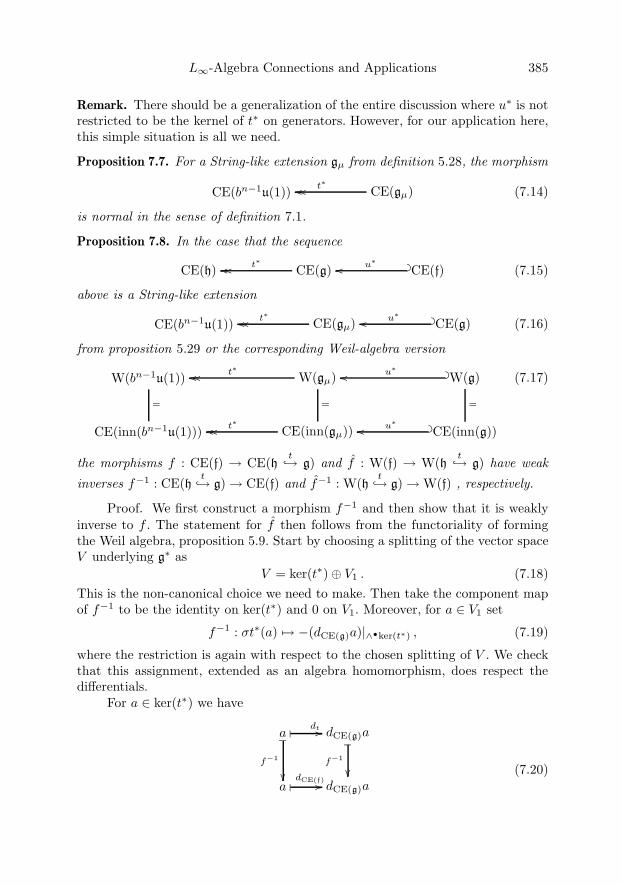
L∞-Algebra Connections and Applications 385
Remark. There should be a generalization of the entire discussion where u∗ is notrestricted to be the kernel of t∗ on generators. However, for our application here,this simple situation is all we need.
Proposition 7.7. For a String-like extension gμ from definition 5.28, the morphism
CE(bn−1u(1)) CE(gμ)t∗���� (7.14)
is normal in the sense of definition 7.1.
Proposition 7.8. In the case that the sequence
CE(h) CE(g)t∗���� CE(f)� �u∗�� (7.15)
above is a String-like extension
CE(bn−1u(1)) CE(gμ)t∗���� CE(g)� �u∗�� (7.16)
from proposition 5.29 or the corresponding Weil-algebra version
W(bn−1u(1))
=
W(gμ)
=
t∗���� W(g)
=
� �u∗��
CE(inn(bn−1u(1))) CE(inn(gμ))t∗���� CE(inn(g))� �u∗��
(7.17)
the morphisms f : CE(f) → CE(ht↪→ g) and f : W(f) → W(h
t↪→ g) have weak
inverses f−1 : CE(ht↪→ g) → CE(f) and f−1 : W(h
t↪→ g) → W(f) , respectively.
Proof. We first construct a morphism f−1 and then show that it is weaklyinverse to f . The statement for f then follows from the functoriality of formingthe Weil algebra, proposition 5.9. Start by choosing a splitting of the vector spaceV underlying g∗ as
V = ker(t∗)⊕ V1 . (7.18)This is the non-canonical choice we need to make. Then take the component mapof f−1 to be the identity on ker(t∗) and 0 on V1. Moreover, for a ∈ V1 set
f−1 : σt∗(a) �→ −(dCE(g)a)|∧•ker(t∗) , (7.19)
where the restriction is again with respect to the chosen splitting of V . We checkthat this assignment, extended as an algebra homomorphism, does respect thedifferentials.
For a ∈ ker(t∗) we have
a � dt ���
f−1
��
dCE(g)a�
f−1
��a � dCE(f)�� dCE(g)a
(7.20)

386 Hisham Sati, Urs Schreiber and Jim Stasheff
using the fact that t∗ is normal. For a ∈ V1 we have
a � dt ���
f−1
��
dCE(g)a + σt∗(a)�
f−1
��0 � dCE(f)�� (dCE(g)a)|∧•ker(t∗) − (dCE(g)a)|∧•ker(t∗)
. (7.21)
and
σt∗(a) � dt ���
f−1
��
−σt∗(dCE(g)a)�
f−1
��−(dCE(g)a)|∧•ker(t∗)
� dCE(f)�� −dCE(f)((dCE(g)a)|ker(t∗)). (7.22)
This last condition happens to be satisfied for the examples stated in the proposi-tion. The details for that are discussed in 7.1.1 below. By the above, f−1 is indeeda morphism of qDGCAs.
Next we check that f−1 is a weak inverse of f . Clearly
CE(f) CE(ht↪→ g)�� CE(f)�� (7.23)
is the identity on CE(f). What remains is to construct a homotopy
CE(ht↪→ g) CE(f)�� CE(h
t↪→ g)��
Id
'(τ
. (7.24)
One checks that this is accomplished by taking τ to act on σV1 as τ : σV1�→ V1
and extended suitably. �
7.1.1. Examples.
Weak cokernel for the String-like extension. Let our sequence
CE(h) CE(g)t∗���� CE(f)� �u∗�� (7.25)
be a String-like extension
CE(bn−1u(1)) CE(gμ)t∗���� CE(g)� �u∗�� (7.26)
from proposition 5.29. Then the mapping cone Chevalley-Eilenberg algebra
CE(bn−1u(1) ↪→ gμ) (7.27)
is∧•(g∗ ⊕ R[n]⊕ R[n + 1]) (7.28)

L∞-Algebra Connections and Applications 387
with differential given by
dt|g∗ = dCE(g) (7.29)dt|R[n] = −μ + σ (7.30)
dt|R[n+1] = 0 . (7.31)
(As always, σ is the canonical degree shifting isomorphism on generators extendedas a derivation.) The morphism
CE(g) CE(bn−1u(1) ↪→ gμ)f−1
��� (7.32)
acts as
f−1|g∗ = Id (7.33)
f−1|R[n] = 0 (7.34)
f−1|R[n+1] = μ . (7.35)
To check the condition in equation (7.22) explicitly in this case, let b ∈ R[n] andwrite b := t∗b for simplicity (since t∗ is the identity on R[n]). Then
σb� dt ��
f−1
��
0
f−1
��μ �dCE(g) �� 0
(7.36)
does commute.Weak cokernel for the String-like extension in terms of the Weil algebra. We willalso need the analogous discussion not for the Chevalley-Eilenberg algebras, butfor the corresponding Weil algebras. To that end consider now the sequence
W(bn−1u(1)) W(gμ)t∗���� W(g)� �u∗�� . (7.37)
This is handled most conveniently by inserting the isomorphism
W(gμ) � CE(csP (g)) (7.38)
from proposition 5.30 as well as the identification
W(g) = CE(inn(g)) (7.39)
such that we get
CE(inn(bn−1u(1))) CE(csP (g))t∗���� CE(inn(g))� �u∗�� . (7.40)
Then we find that the mapping cone algebra CE(bn−1u(1) ↪→ csP (g)) is
∧•(g∗ ⊕ g∗[1]⊕ (R[n]⊕ R[n + 1])⊕ (R[n + 1]⊕ R[n + 2])) . (7.41)
Write b and c for the canonical basis elements of R[n]⊕R[n+1], then the differentialis characterized by
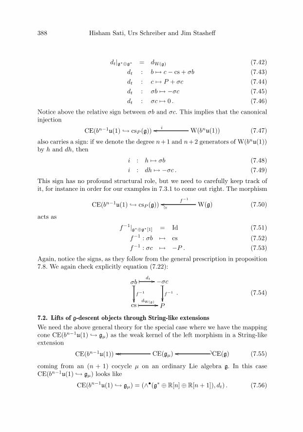
388 Hisham Sati, Urs Schreiber and Jim Stasheff
dt|g∗⊕g∗ = dW(g) (7.42)dt : b �→ c− cs + σb (7.43)dt : c �→ P + σc (7.44)dt : σb �→ −σc (7.45)dt : σc �→ 0 . (7.46)
Notice above the relative sign between σb and σc. This implies that the canonicalinjection
CE(bn−1u(1) ↪→ csP (g)) W(bnu(1))i�� (7.47)
also carries a sign: if we denote the degree n+1 and n+2 generators of W(bnu(1))by h and dh, then
i : h �→ σb (7.48)i : dh �→ −σc . (7.49)
This sign has no profound structural role, but we need to carefully keep track ofit, for instance in order for our examples in 7.3.1 to come out right. The morphism
CE(bn−1u(1) ↪→ csP (g)) W(g)f−1
��� (7.50)
acts as
f−1|g∗⊕g∗[1] = Id (7.51)
f−1 : σb �→ cs (7.52)f−1 : σc �→ −P . (7.53)
Again, notice the signs, as they follow from the general prescription in proposition7.8. We again check explicitly equation (7.22):
σb� dt ��
�
f−1
��
−σc�
f−1
��cs � dW(g) �� P
. (7.54)
7.2. Lifts of g-descent objects through String-like extensions
We need the above general theory for the special case where we have the mappingcone CE(bn−1u(1) ↪→ gμ) as the weak kernel of the left morphism in a String-likeextension
CE(bn−1u(1)) CE(gμ)���� CE(g)� ��� (7.55)
coming from an (n + 1) cocycle μ on an ordinary Lie algebra g. In this caseCE(bn−1u(1) ↪→ gμ) looks like
CE(bn−1u(1) ↪→ gμ) = (∧•(g∗ ⊕ R[n]⊕ R[n + 1]), dt) . (7.56)

L∞-Algebra Connections and Applications 389
By chasing this through the above definitions, we find
Proposition 7.9. The morphism
f−1 : CE(bn−1u(1) ↪→ gμ) → CE(g) (7.57)
acts as the identity on g∗
f−1|g∗ = Id , (7.58)vanishes on R[n]
f−1|R[n] : b �→ 0, (7.59)and satisfies
f−1|R[n+1] : σt∗b �→ μ . (7.60)
Therefore we find the (n + 1)-cocycle
Ω•vert(Y ) CE(bnu(1))
Avert�� (7.61)
obstructing the lift of a g-cocycle
Ω•vert(Y ) CE(g)
Avert�� , (7.62)
according to 2.3 given by
CE(bn−1u(1) ↪→ gμ)
������
����
f−1
��
CE(bnu(1))� �j��
Avert���������
���������CE(bn−1u(1)) CE(gμ)i∗����
��
CE(g)� ���
Avert
��ٕ
vert(Y )
, (7.63)
to be the (n + 1)-formμ(Avert) ∈ Ωn+1
vert (Y ) . (7.64)
Proposition 7.10. Let Avert ∈ Ω1vert(Y, g) be the cocycle of a G-bundle P → X
for g semisimple and let μ = 〈·, [·, ·]〉 be the canonical 3-cocycle. Then gμ is thestandard String Lie 3-algebra and the obstruction to lifting P to a String 2-bundle,i.e. lifting to a gμ-cocycle, is the Chern-Simons 3-bundle with cocycle given by thevertical 3-form
〈Avert ∧ [Avert ∧Avert]〉 ∈ Ω3vert(Y ) . (7.65)
In the following we will express these obstruction in a more familiar way interms of their characteristic classes. In order to do that, we first need to generalizethe discussion to differential g-cocycle. But that is now straightforward.
7.2.1. Examples. The continuation of the discussion of 5.3.1 to coset spaces givesa classical illustration of the lifting construction considered here.
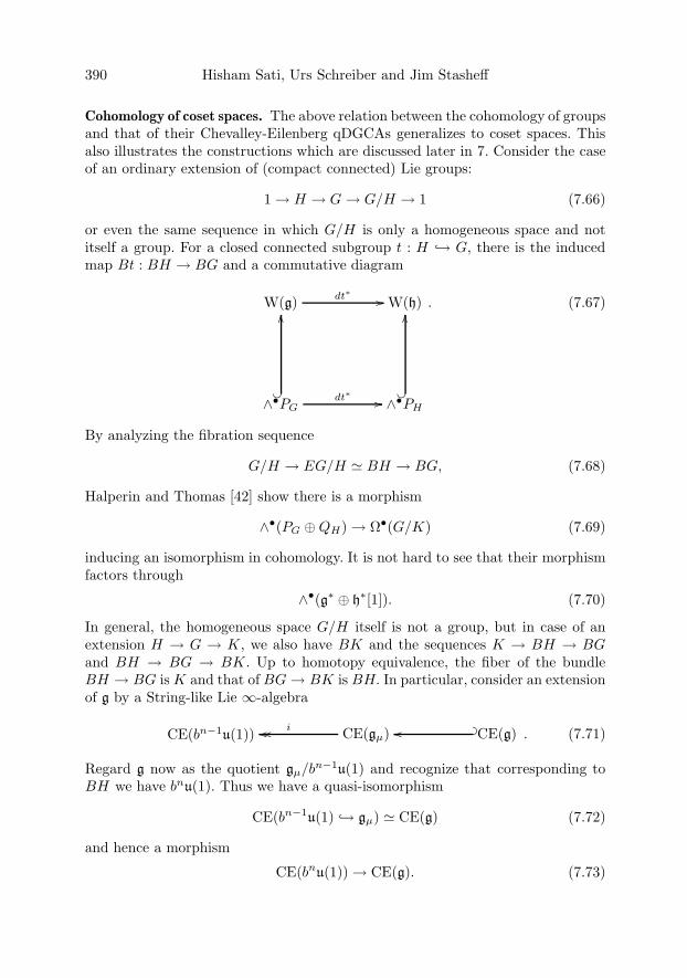
390 Hisham Sati, Urs Schreiber and Jim Stasheff
Cohomology of coset spaces. The above relation between the cohomology of groupsand that of their Chevalley-Eilenberg qDGCAs generalizes to coset spaces. Thisalso illustrates the constructions which are discussed later in 7. Consider the caseof an ordinary extension of (compact connected) Lie groups:
1 → H → G→ G/H → 1 (7.66)
or even the same sequence in which G/H is only a homogeneous space and notitself a group. For a closed connected subgroup t : H ↪→ G, there is the inducedmap Bt : BH → BG and a commutative diagram
W(g) dt∗ �� W(h)
∧•PGdt∗ ����
��
∧•PH
��
��. (7.67)
By analyzing the fibration sequence
G/H → EG/H � BH → BG, (7.68)
Halperin and Thomas [42] show there is a morphism
∧•(PG ⊕QH) → Ω•(G/K) (7.69)
inducing an isomorphism in cohomology. It is not hard to see that their morphismfactors through
∧•(g∗ ⊕ h∗[1]). (7.70)
In general, the homogeneous space G/H itself is not a group, but in case of anextension H → G → K, we also have BK and the sequences K → BH → BGand BH → BG → BK. Up to homotopy equivalence, the fiber of the bundleBH → BG is K and that of BG→ BK is BH. In particular, consider an extensionof g by a String-like Lie ∞-algebra
CE(bn−1u(1)) CE(gμ)i���� CE(g)� ��� . (7.71)
Regard g now as the quotient gμ/bn−1u(1) and recognize that corresponding to
BH we have bnu(1). Thus we have a quasi-isomorphism
CE(bn−1u(1) ↪→ gμ) � CE(g) (7.72)
and hence a morphism
CE(bnu(1)) → CE(g). (7.73)
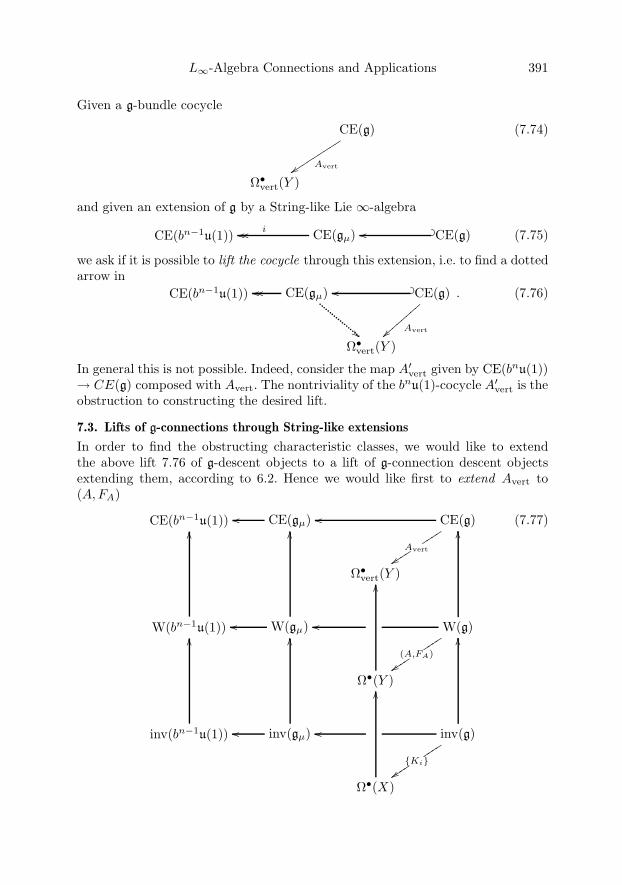
L∞-Algebra Connections and Applications 391
Given a g-bundle cocycle
CE(g)
Avert�������
����
Ω•vert(Y )
(7.74)
and given an extension of g by a String-like Lie ∞-algebra
CE(bn−1u(1)) CE(gμ)i���� CE(g)� ��� (7.75)
we ask if it is possible to lift the cocycle through this extension, i.e. to find a dottedarrow in
CE(bn−1u(1)) CE(gμ)����
��
CE(g)� ���
Avert��������
Ω•vert(Y )
. (7.76)
In general this is not possible. Indeed, consider the map A′vert given by CE(bnu(1))
→ CE(g) composed with Avert. The nontriviality of the bnu(1)-cocycle A′vert is the
obstruction to constructing the desired lift.
7.3. Lifts of g-connections through String-like extensions
In order to find the obstructing characteristic classes, we would like to extendthe above lift 7.76 of g-descent objects to a lift of g-connection descent objectsextending them, according to 6.2. Hence we would like first to extend Avert to(A,FA)
CE(bn−1u(1)) ����
CE(gμ) ����
CE(g)��
Ω•vert(Y )
��Avert����
����
��
W(bn−1u(1)) ����
W(gμ) ����
W(g)��
ٕ(Y )��
(A,FA)����
����
��
inv(bn−1u(1)) �� inv(gμ) �� inv(g)
ٕ(X)��
{Ki}����
����
(7.77)
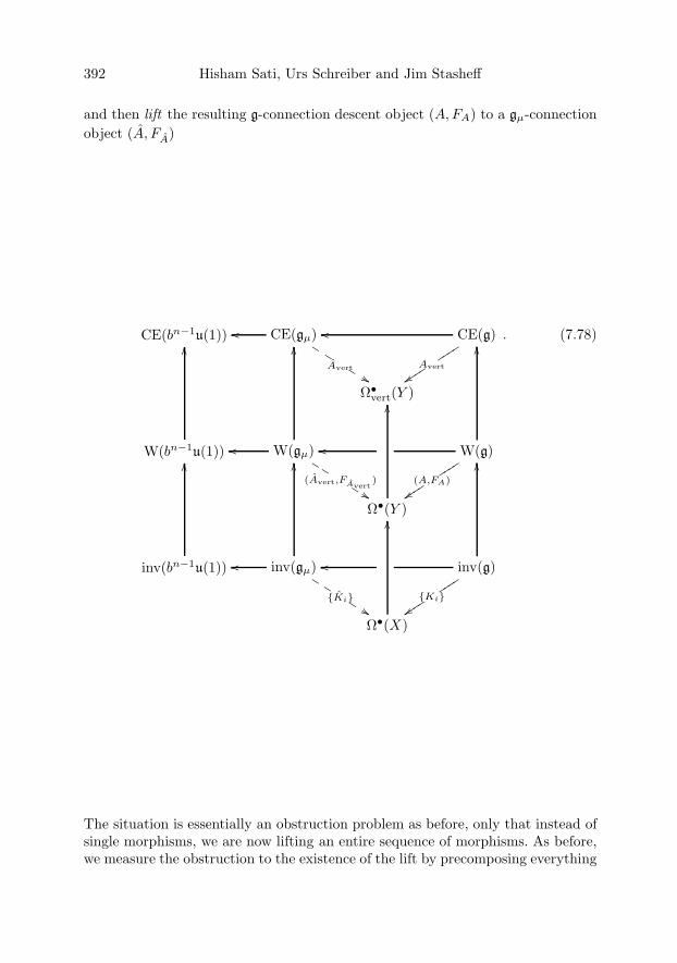
392 Hisham Sati, Urs Schreiber and Jim Stasheff
and then lift the resulting g-connection descent object (A,FA) to a gμ-connectionobject (A, FA)
CE(bn−1u(1)) ����
CE(gμ) ����
CE(g)��
Ω•vert(Y )
��Avert����
����
��
*+Avert�
�
��
W(bn−1u(1)) ����
W(gμ) ����
W(g)��
ٕ(Y )��
(A,FA)����
����
��
*+(Avert,FAvert
)� �
� �
inv(bn−1u(1)) �� inv(gμ) �� inv(g)
ٕ(X)��
{Ki}����
����
*+{Ki}�
�
� �
. (7.78)
The situation is essentially an obstruction problem as before, only that instead ofsingle morphisms, we are now lifting an entire sequence of morphisms. As before,we measure the obstruction to the existence of the lift by precomposing everything
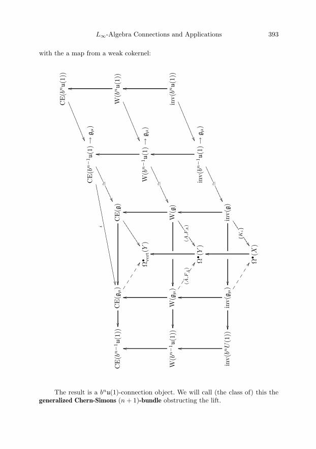
L∞-Algebra Connections and Applications 393
with the a map from a weak cokernel:C
E(b
nu(1
))��
CE
(bn−
1u(1
)→
gμ)
!"
� � � � � � � � � � � � �
��
CE
(bn−
1u(1
))��
��C
E(g
μ)��
��+,
i� � � � � � � � � � � � � � � � � � � � � � � � � � � � � � �
CE
(g)
��
��� � � � � � �
� � � � �
W(b
nu(1
))��
Ω• vert(Y
)��
� � � � � � � � � �*+
��
��
�
��W
(bn−
1u(1
)→
gμ)
!"
� � � � � � � � � � � � �
��
W(b
n−
1u(1
))��
��W
(gμ)��
��W
(g)��
� � � � � � �
� � � � �
��in
v(bn
u(1
))
Ω• (Y
)��(A
,FA
)� � � �
� � � �
*+(A
,FA
) ��
��
��in
v(bn
−1u(1
)→
gμ)
!"
� � � � � � � � � � � � �
inv(bnU
(1))
��in
v(g
μ)��
inv(
g)��
� � � � � � �
� � � � �
Ω• (X
)��{K
i}
� � � �
� � � �
*+
��
��
�
The result is a bnu(1)-connection object. We will call (the class of) this thegeneralized Chern-Simons (n + 1)-bundle obstructing the lift.

394 Hisham Sati, Urs Schreiber and Jim Stasheff
CE
(bnu(1
))��
CS(A
) ver
t
,-
CE
(bn−
1u(1
)→
gμ)
!"
� � � � � � � � � � � � �
��
CE
(bn−
1u(1
))��
��C
E(g
μ)��
��+,
i� � � � � � � � � � � � � � � � � � � � � � � � � � � � � � �
CE
(g)
��
��� � � � � � �
� � � � �
W(b
nu(1
))��
(CS(A
),P
(FA
))
,-
Ω• vert(Y
)��
� � � � � � � � � �*+
��
��
�
��W
(bn−
1u(1
)→
gμ)
!"
� � � � � � � � � � � � �
��
W(b
n−
1u(1
))��
��W
(gμ)��
��W
(g)��
� � � � � � �
� � � � �
��in
v(bn
u(1
))
{P(F
A)}
,-
Ω• (Y
)��(A
,FA
)� � � �
� � � �
*+(A
,FA
) ��
��
��in
v(bn
−1u(1
)→
gμ)
!"
� � � � � � � � � � � � �
inv(bnU
(1))
��in
v(g
μ)��
inv(
g)��
� � � � � � �
� � � � �
Ω• (X
)��{K
i}
� � � �
� � � �
*+
��
��
�
Figure 12. The generalized Chern-Simons bnu(1)-bundle thatobstructs the lift of a given g-bundle to a gμ-bundle, or ratherthe descent object representing it.

L∞-Algebra Connections and Applications 395
In order to construct the lift it is convenient, for similar reasons as in the proofof proposition 5.32, to work with CE(csP (g)) instead of the isomorphic W(gμ),using the isomorphism from proposition 5.30. Furthermore, using the identity
W(g) = CE(inn(g)) (7.79)
mentioned in 5.1, we can hence consider instead of
W(bn−1) W(gμ)���� W(g)� ��� (7.80)
the sequence
CE(inn(bn−1)) CE(csP (g))���� CE(inn(g))� ��� . (7.81)
Fortunately, this still satisfies the assumptions of proposition 7.6. So in completeanalogy, we find the extension of proposition 7.9 from g-bundle cocycles to differ-ential g-cocycles:
Proposition 7.11. The morphism
f−1 : CE(inn(bn−1u(1)) ↪→ CE(csP (g)) → CE(inn(g)) (7.82)
constructed as in proposition 7.9 acts as the identity on g∗ ⊕ g∗[1]
f−1|g∗⊕g∗[1] = Id (7.83)
and satisfiesf−1|R[n+2] : c �→ P . (7.84)
This means that, as an extension of proposition 7.10, we find the differentialbnu(1) (n + 1)-cocycle
ٕ(Y ) W(bnu(1))A�� (7.85)
obstructing the lift of a differential g-cocycle
ٕ(Y ) W(g)(A,FA)�� , (7.86)
according to the above discussion
CE(inn(bn−1u(1)) ↪→ inn(gμ))
!"������
������
�f−1
��
W(bnu(1))� �j��
(A,FA)����������
������������
W(bn−1u(1)) W(gμ)i∗����
-.
W(g)� ���
(A,FA)
��ٕ(Y )
,
(7.87)to be the connection (n + 1)-form
A = CS(A) ∈ Ωn+1(Y ) (7.88)
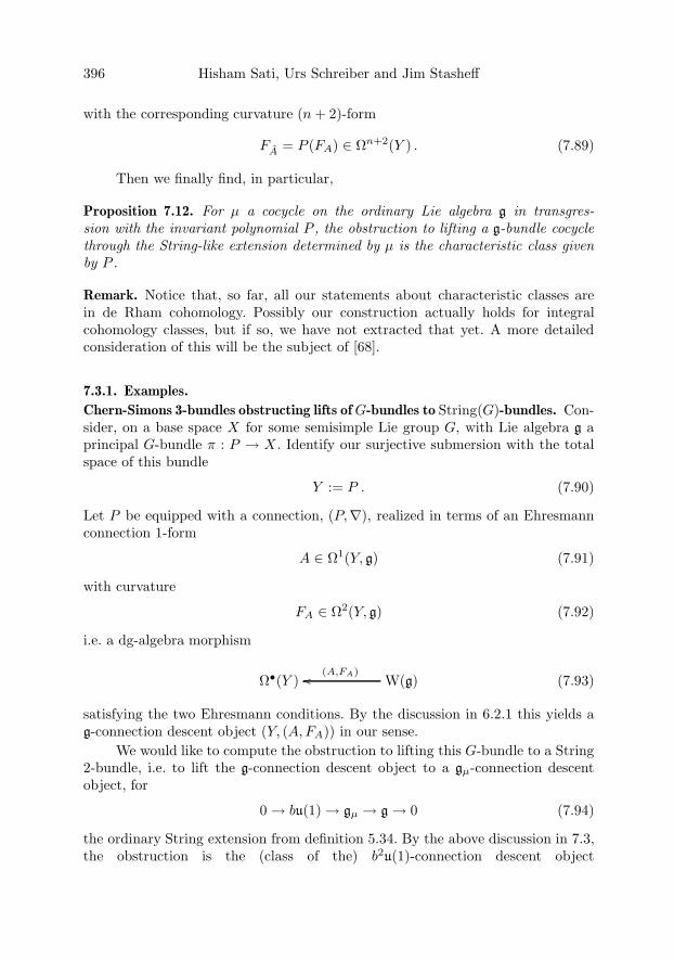
396 Hisham Sati, Urs Schreiber and Jim Stasheff
with the corresponding curvature (n + 2)-form
FA = P (FA) ∈ Ωn+2(Y ) . (7.89)
Then we finally find, in particular,
Proposition 7.12. For μ a cocycle on the ordinary Lie algebra g in transgres-sion with the invariant polynomial P , the obstruction to lifting a g-bundle cocyclethrough the String-like extension determined by μ is the characteristic class givenby P .
Remark. Notice that, so far, all our statements about characteristic classes arein de Rham cohomology. Possibly our construction actually holds for integralcohomology classes, but if so, we have not extracted that yet. A more detailedconsideration of this will be the subject of [68].
7.3.1. Examples.
Chern-Simons 3-bundles obstructing lifts ofG-bundles to String(G)-bundles. Con-sider, on a base space X for some semisimple Lie group G, with Lie algebra g aprincipal G-bundle π : P → X . Identify our surjective submersion with the totalspace of this bundle
Y := P . (7.90)
Let P be equipped with a connection, (P,∇), realized in terms of an Ehresmannconnection 1-form
A ∈ Ω1(Y, g) (7.91)
with curvature
FA ∈ Ω2(Y, g) (7.92)
i.e. a dg-algebra morphism
ٕ(Y ) W(g)(A,FA)�� (7.93)
satisfying the two Ehresmann conditions. By the discussion in 6.2.1 this yields ag-connection descent object (Y, (A,FA)) in our sense.
We would like to compute the obstruction to lifting this G-bundle to a String2-bundle, i.e. to lift the g-connection descent object to a gμ-connection descentobject, for
0 → bu(1) → gμ → g → 0 (7.94)
the ordinary String extension from definition 5.34. By the above discussion in 7.3,the obstruction is the (class of the) b2u(1)-connection descent object

L∞-Algebra Connections and Applications 397
(Y, (H(3), G(4))) whose connection and curvature are given by the composite
W(b2u(1))
(H(3),G(4))
./
(W(bu(1)) → CE(csP (g)))&'
��������������
W(g)!"
��������
������
ٕ(Y )��(A,FA)���
���
, (7.95)
where, as discussed above, we are making use of the isomorphism W(gμ) �CE(csP (g)) from proposition 5.30. The crucial aspect of this composite is theisomorphism
W(g) (W(bu(1)) → CEP (g))f−1
��� (7.96)
from proposition 7.8. This is where the obstruction data is picked up. The im-portant formula governing this is equation (7.19), which describes how the shiftedelements coming from W(bu(1)) in the mapping cone (W(bu(1)) → CEP (g)) aremapped to W(g).
Recall that W(b2u(1)) = F(R[3]) is generated from elements (h, dh) of degree3 and 4, respectively, that W(bu(1)) = F(R[2]) is generated from elements (c, dc)of degree 2 and 3, respectively, and that CE(csP (g)) is generated from g∗ ⊕ g∗[1]together with elements b and c of degree 2 and 3, respectively, with
dCE(csP (g))b = c− cs (7.97)
and
dCE(csP (g))c = P , (7.98)
where cs ∈ ∧3(g∗ ⊕ g∗[1]) is the transgression element interpolating between thecocycle μ = 〈·, [·, ·]〉 ∈ ∧3(g∗) and the invariant polynomial P = 〈·, ·〉 ∈ ∧2(g∗[1]).Hence the map f−1 acts as
f−1 : σb �→ −(dCE(csP (g))b)|∧•(g∗⊕g∗[1]) = +cs (7.99)
and
f−1 : σc �→ −(dCE(csP (g))c)|∧•(g∗⊕g∗[1]) = −P . (7.100)

398 Hisham Sati, Urs Schreiber and Jim Stasheff
Therefore the above composite (H(3), G(4)) maps the generators (h, dh) ofW(b2u(1)) as
h�
(H(3),G(4))
./
σb&'
�����������������
cs &'����������
������
CSP (FA)��(A,FA)���
�����
(7.101)
and
dh�
(H(3),G(4))
./
-σc&'
����������������
P&'
����������
�������
P (FA)��(A,FA)���
����
. (7.102)
Notice the signs here, as discussed around equation (7.47). We then have that theconnection 3-form of the Chern-Simons 3-bundle given by our obstructing b2u(1)-connection descent object is the Chern-Simons form
H(3) = −CS(A,FA) = −〈A ∧ dA〉 − 13〈A ∧ [A ∧A]〉 ∈ Ω3(Y ) (7.103)
of the original Ehresmann connection 1-form A, and its 4-form curvature is there-fore the corresponding 4-form
G(4) = −P (FA) = 〈FA ∧ FA〉 ∈ Ω4(Y ) . (7.104)
This descends down to X , where it constitutes the characteristic form which clas-sifies the obstruction. Indeed, noticing that inv(b2u(1)) = ∧•(R[4]), we see that(this works the same for all line n-bundles, i.e., for all bn−1u(1)-connection descent

L∞-Algebra Connections and Applications 399
objects) the characteristic forms of the obstructing Chern-Simons 3-bundle
inv(b2u(1))
{G(4)}
./
inv(bu(1) → gμ)!"
������������
inv(g)��
�!!!!!
!!!!!
ٕ(X)��
{Ki}���
���
(7.105)
consist only and precisely of this curvature 4-form: the second Chern-form of theoriginal G-bundle P .
8. L∞-algebra parallel transport
One of the main points about a connection is that it allows to do parallel transport.Connections on ordinary bundles give rise to a notion of parallel transport alongcurves, known as holonomy if these curves are closed.
Higher connections on n-bundles should yield a way to obtain a notion ofparallel transport over n-dimensional spaces. In physics, this assignment plays therole of the gauge coupling term in the non-kinetic part of the action functional:the action functional of the charged particle is essentially its parallel transportwith respect to an ordinary (1-)connection, while the action functional of thestring contains the parallel transport of a 2-connection (the Kalb-Ramond field).Similarly the action functional of the membrane contains the parallel transport ofa 3-connection (the supergravity “C-field”).
There should therefore be a way to assign to any one of our g-connectiondescent objects for g any Lie n-algebra
• a prescription for parallel transport over n-dimensional spaces;• a configuration space for the n-particle coupled to that transport;• a way to transgress the transport to an action functional on that configuration
space;• a way to obtain the corresponding quantum theory.
Each point deserves a separate discussion, but in the remainder we shallquickly give an impression for how each of these points is addressed in our context.
8.1. L∞-parallel transport
In this section we indicate briefly how our notion of g-connections give rise to anotion of parallel transport over n-dimensional spaces. The abelian case (meaning
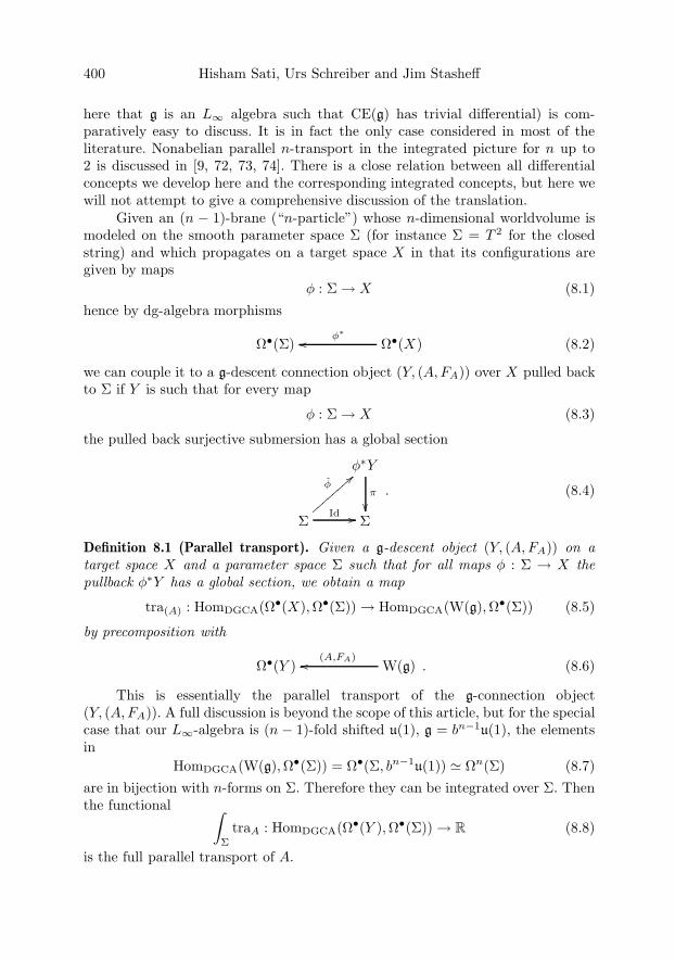
400 Hisham Sati, Urs Schreiber and Jim Stasheff
here that g is an L∞ algebra such that CE(g) has trivial differential) is com-paratively easy to discuss. It is in fact the only case considered in most of theliterature. Nonabelian parallel n-transport in the integrated picture for n up to2 is discussed in [9, 72, 73, 74]. There is a close relation between all differentialconcepts we develop here and the corresponding integrated concepts, but here wewill not attempt to give a comprehensive discussion of the translation.
Given an (n − 1)-brane (“n-particle”) whose n-dimensional worldvolume ismodeled on the smooth parameter space Σ (for instance Σ = T 2 for the closedstring) and which propagates on a target space X in that its configurations aregiven by maps
φ : Σ → X (8.1)
hence by dg-algebra morphisms
Ω•(Σ) Ω•(X)φ∗
�� (8.2)
we can couple it to a g-descent connection object (Y, (A,FA)) over X pulled backto Σ if Y is such that for every map
φ : Σ → X (8.3)
the pulled back surjective submersion has a global section
φ∗Y
π
��Σ
Id ��
φ/0��������Σ
. (8.4)
Definition 8.1 (Parallel transport). Given a g-descent object (Y, (A,FA)) on atarget space X and a parameter space Σ such that for all maps φ : Σ → X thepullback φ∗Y has a global section, we obtain a map
tra(A) : HomDGCA(Ω•(X),Ω•(Σ)) → HomDGCA(W(g),Ω•(Σ)) (8.5)
by precomposition with
ٕ(Y ) W(g)(A,FA)�� . (8.6)
This is essentially the parallel transport of the g-connection object(Y, (A,FA)). A full discussion is beyond the scope of this article, but for the specialcase that our L∞-algebra is (n − 1)-fold shifted u(1), g = bn−1u(1), the elementsin
HomDGCA(W(g),Ω•(Σ)) = Ω•(Σ, bn−1u(1)) � Ωn(Σ) (8.7)are in bijection with n-forms on Σ. Therefore they can be integrated over Σ. Thenthe functional ∫
Σ
traA : HomDGCA(Ω•(Y ),Ω•(Σ)) → R (8.8)
is the full parallel transport of A.
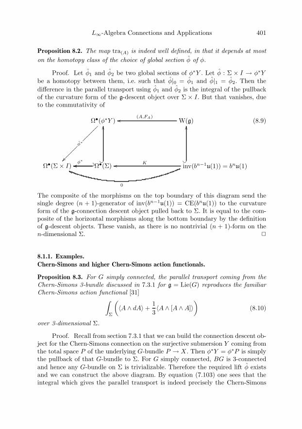
L∞-Algebra Connections and Applications 401
Proposition 8.2. The map tra(A) is indeed well defined, in that it depends at moston the homotopy class of the choice of global section φ of φ.
Proof. Let φ1 and φ2 be two global sections of φ∗Y . Let φ : Σ × I → φ∗Ybe a homotopy between them, i.e. such that φ|0 = φ1 and φ|1 = φ2. Then thedifference in the parallel transport using φ1 and φ2 is the integral of the pullbackof the curvature form of the g-descent object over Σ × I. But that vanishes, dueto the commutativity of
Ω•(φ∗Y )
φ∗�������
01�������
W(g)(A,FA)��
Ω•(Σ× I) Ω•(Σ)� �����
��
φ∗�� inv(bn−1u(1)) = bnu(1)
0
12
��
��
K��
(8.9)
The composite of the morphisms on the top boundary of this diagram send thesingle degree (n + 1)-generator of inv(bn−1u(1)) = CE(bnu(1)) to the curvatureform of the g-connection descent object pulled back to Σ. It is equal to the com-posite of the horizontal morphisms along the bottom boundary by the definitionof g-descent objects. These vanish, as there is no nontrivial (n + 1)-form on then-dimensional Σ. �
8.1.1. Examples.
Chern-Simons and higher Chern-Simons action functionals.
Proposition 8.3. For G simply connected, the parallel transport coming from theChern-Simons 3-bundle discussed in 7.3.1 for g = Lie(G) reproduces the familiarChern-Simons action functional [31]∫
Σ
(〈A ∧ dA〉+
13〈A ∧ [A ∧A]〉
)(8.10)
over 3-dimensional Σ.
Proof. Recall from section 7.3.1 that we can build the connection descent ob-ject for the Chern-Simons connection on the surjective submersion Y coming fromthe total space P of the underlying G-bundle P → X . Then φ∗Y = φ∗P is simplythe pullback of that G-bundle to Σ. For G simply connected, BG is 3-connectedand hence any G-bundle on Σ is trivializable. Therefore the required lift φ existsand we can construct the above diagram. By equation (7.103) one sees that theintegral which gives the parallel transport is indeed precisely the Chern-Simons
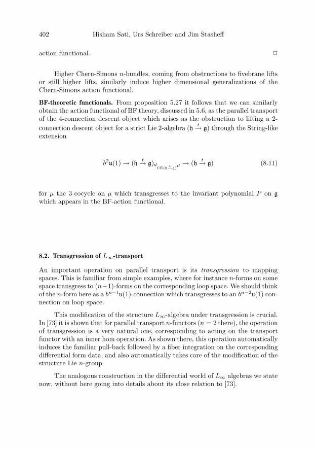
402 Hisham Sati, Urs Schreiber and Jim Stasheff
action functional. �
Higher Chern-Simons n-bundles, coming from obstructions to fivebrane liftsor still higher lifts, similarly induce higher dimensional generalizations of theChern-Simons action functional.
BF-theoretic functionals. From proposition 5.27 it follows that we can similarlyobtain the action functional of BF theory, discussed in 5.6, as the parallel transportof the 4-connection descent object which arises as the obstruction to lifting a 2-connection descent object for a strict Lie 2-algebra (h t→ g) through the String-likeextension
b2u(1) → (h t→ g)dCE(h t→g)
μ → (h t→ g) (8.11)
for μ the 3-cocycle on μ which transgresses to the invariant polynomial P on gwhich appears in the BF-action functional.
8.2. Transgression of L∞-transport
An important operation on parallel transport is its transgression to mappingspaces. This is familiar from simple examples, where for instance n-forms on somespace transgress to (n−1)-forms on the corresponding loop space. We should thinkof the n-form here as a bn−1u(1)-connection which transgresses to an bn−2u(1) con-nection on loop space.
This modification of the structure L∞-algebra under transgression is crucial.In [73] it is shown that for parallel transport n-functors (n = 2 there), the operationof transgression is a very natural one, corresponding to acting on the transportfunctor with an inner hom operation. As shown there, this operation automaticallyinduces the familiar pull-back followed by a fiber integration on the correspondingdifferential form data, and also automatically takes care of the modification of thestructure Lie n-group.
The analogous construction in the differential world of L∞ algebras we statenow, without here going into details about its close relation to [73].
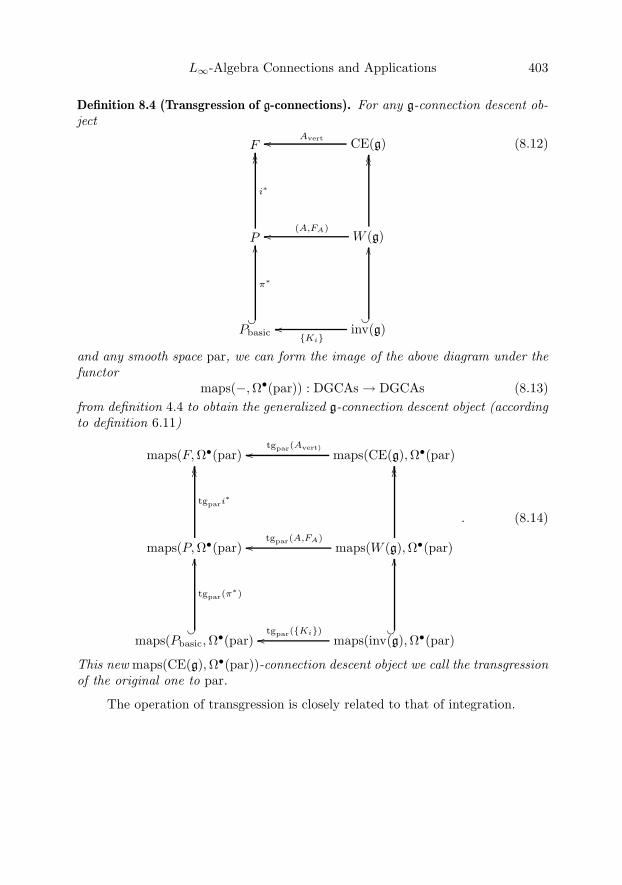
L∞-Algebra Connections and Applications 403
Definition 8.4 (Transgression of g-connections). For any g-connection descent ob-ject
F CE(g)Avert��
P
i∗
����
W (g)
����
(A,FA)��
Pbasic
��
π∗
��
inv(g)��
��
{Ki}��
(8.12)
and any smooth space par, we can form the image of the above diagram under thefunctor
maps(−,Ω•(par)) : DGCAs → DGCAs (8.13)from definition 4.4 to obtain the generalized g-connection descent object (accordingto definition 6.11)
maps(F,ٕ(par) maps(CE(g),ٕ(par)tgpar(Avert)��
maps(P,Ω•(par)
tgpari∗
����
maps(W (g),Ω•(par)
����
tgpar(A,FA)��
maps(Pbasic,ٕ(par)��
tgpar(π∗)
��
maps(inv(g),ٕ(par)��
��
tgpar({Ki})��
. (8.14)
This new maps(CE(g),Ω•(par))-connection descent object we call the transgressionof the original one to par.
The operation of transgression is closely related to that of integration.

404 Hisham Sati, Urs Schreiber and Jim Stasheff
8.2.1. Examples.Transgression of bn−1u(1)-connections. Let g be an L∞-algebra of the form shiftedu(1), g = bn−1u(1). By proposition 5.25 the Weil algebra W(bn−1u(1)) is the freeDGCA on a single degree n-generator b with differential c := db. Recall from 5.5.1that a DGCA morphism W(bn−1u(1)) → Ω•(Y ) is just an n-form on Y . For everypoint y ∈ par and for every multivector v ∈ ∧nTypar we get a 0-form on thesmooth space
maps(W(bn−1u(1)),Ω•(par)) (8.15)
of all n-forms on par, which we denote
A(v) ∈ Ω(maps(W(bn−1u(1)),Ω•(par))) . (8.16)
This is the 0-form on this space of maps obtained from the element b ∈ W(bn−1u(1))and the current δy (the ordinary delta-distribution on 0-forms) according to propo-sition 4.6. Its value on any n-form ω is the value of that form evaluated on v.
Since this, and its generalizations which we discuss in 8.3.1, is crucial formaking contact with standard constructions in physics, it may be worthwhile torepeat that statement more explicitly in terms of components: Assume that par =Rk and for any point y let v be the unit in ∧T nRn � R. Then A(v) is the 0-formon the space of forms which sends any form ω = ωμ1μ2...μndx
μ1 ∧ · · · ∧ dxμn to itscomponent
A(v) : ω �→ ω(y)12···n . (8.17)
This implies that when a bn−1u(1)-connection is transgressed to the space of mapsfrom an n-dimensional parameter space par, it becomes a map that pulls backfunctions on the space of n-forms on par to the space of functions on maps fromparameter space into target space. But such pullbacks correspond to functions(0-forms) on the space of maps par → tar with values in the space of n-forms ontra.
8.3. Configuration spaces of L∞-transport
With the notion of g-connections and their parallel transport and transgressionin hand, we can say what it means to couple an n-particle/(n − 1)-brane to ag-connection.
Definition 8.5 (The charged n-particle/(n−1)-brane). We say a charged n-particle/(n− 1)-brane is a tuple (par, (A,FA)) consisting of• parameter space par: a smooth space• a background field (A,FA): a g-connection descent object involving
– target space tar: the smooth space– space!target that the g-connection (A,FA) lives over;– space of phases phas: the smooth space such that Ω•(phas) � CE(g)
From such a tuple we form• configuration space• configuration space conf = homS∞(par, tar);
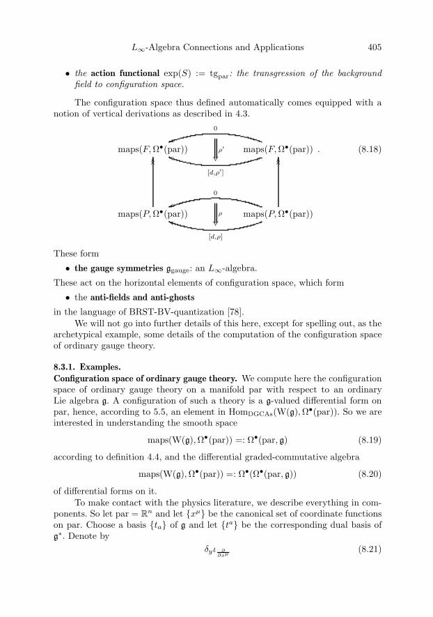
L∞-Algebra Connections and Applications 405
• the action functional exp(S) := tgpar: the transgression of the backgroundfield to configuration space.
The configuration space thus defined automatically comes equipped with anotion of vertical derivations as described in 4.3.
maps(F,Ω•(par)) maps(F,Ω•(par))
[d,ρ′]
12
0
&'
maps(P,Ω•(par))
����
maps(P,Ω•(par))
����
[d,ρ]
12
0
&'
ρ′
ρ
. (8.18)
These form
• the gauge symmetries ggauge: an L∞-algebra.
These act on the horizontal elements of configuration space, which form
• the anti-fields and anti-ghosts
in the language of BRST-BV-quantization [78].We will not go into further details of this here, except for spelling out, as the
archetypical example, some details of the computation of the configuration spaceof ordinary gauge theory.
8.3.1. Examples.
Configuration space of ordinary gauge theory. We compute here the configurationspace of ordinary gauge theory on a manifold par with respect to an ordinaryLie algebra g. A configuration of such a theory is a g-valued differential form onpar, hence, according to 5.5, an element in HomDGCAs(W(g),Ω•(par)). So we areinterested in understanding the smooth space
maps(W(g),Ω•(par)) =: Ω•(par, g) (8.19)
according to definition 4.4, and the differential graded-commutative algebra
maps(W(g),Ω•(par)) =: Ω•(Ω•(par, g)) (8.20)
of differential forms on it.To make contact with the physics literature, we describe everything in com-
ponents. So let par = Rn and let {xμ} be the canonical set of coordinate functionson par. Choose a basis {ta} of g and let {ta} be the corresponding dual basis ofg∗. Denote by
δyι ∂∂xμ
(8.21)
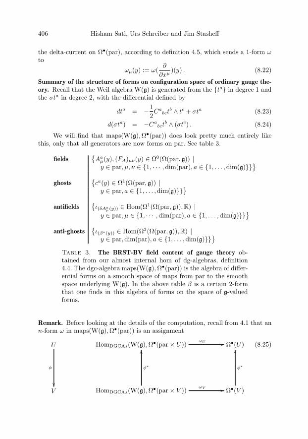
406 Hisham Sati, Urs Schreiber and Jim Stasheff
the delta-current on Ω•(par), according to definition 4.5, which sends a 1-form ωto
ωμ(y) := ω(∂
∂xμ)(y) . (8.22)
Summary of the structure of forms on configuration space of ordinary gauge the-ory. Recall that the Weil algebra W(g) is generated from the {ta} in degree 1 andthe σta in degree 2, with the differential defined by
dta = −12Ca
bctb ∧ tc + σta (8.23)
d(σta) = −Cabct
b ∧ (σtc) . (8.24)
We will find that maps(W(g),Ω•(par)) does look pretty much entirely likethis, only that all generators are now forms on par. See table 3.
fields{Aa
μ(y), (FA)μν(y) ∈ Ω0(Ω(par, g)) |y ∈ par, μ, ν ∈ {1, · · · , dim(par), a ∈ {1, . . . ,dim(g)}}
}ghosts
{ca(y) ∈ Ω1(Ω(par, g)) |y ∈ par, a ∈ {1, . . . ,dim(g)}}
}antifields
{ι(δAa
μ(y)) ∈ Hom(Ω1(Ω(par, g)),R) |y ∈ par, μ ∈ {1, · · · , dim(par), a ∈ {1, . . . ,dim(g)}}
}anti-ghosts
{ι(βa(y)) ∈ Hom(Ω2(Ω(par, g)),R) |y ∈ par, dim(par), a ∈ {1, . . . ,dim(g)}}
}Table 3. The BRST-BV field content of gauge theory ob-tained from our almost internal hom of dg-algebras, definition4.4. The dgc-algebra maps(W(g),Ω•(par)) is the algebra of differ-ential forms on a smooth space of maps from par to the smoothspace underlying W(g). In the above table β is a certain 2-formthat one finds in this algebra of forms on the space of g-valuedforms.
Remark. Before looking at the details of the computation, recall from 4.1 that ann-form ω in maps(W(g),Ω•(par)) is an assignment
U
φ
��
HomDGCAs(W(g),Ω•(par× U))ωU �� Ω•(U)
V HomDGCAs(W(g),Ω•(par× V ))ωV ��
φ∗
��
Ω•(V )
φ∗
��(8.25)
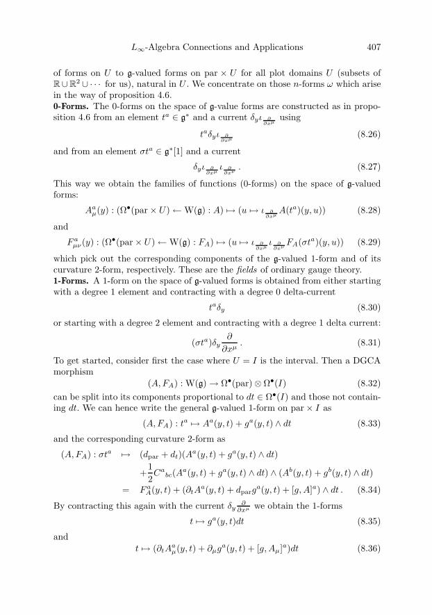
L∞-Algebra Connections and Applications 407
of forms on U to g-valued forms on par × U for all plot domains U (subsets ofR∪R2 ∪ · · · for us), natural in U . We concentrate on those n-forms ω which arisein the way of proposition 4.6.0-Forms. The 0-forms on the space of g-value forms are constructed as in propo-sition 4.6 from an element ta ∈ g∗ and a current δyι ∂
∂xμusing
taδyι ∂∂xμ
(8.26)
and from an element σta ∈ g∗[1] and a current
δyι ∂∂xμ
ι ∂∂xν
. (8.27)
This way we obtain the families of functions (0-forms) on the space of g-valuedforms:
Aaμ(y) : (Ω•(par× U) ← W(g) : A) �→ (u �→ ι ∂
∂xμA(ta)(y, u)) (8.28)
and
F aμν(y) : (Ω•(par× U) ← W(g) : FA) �→ (u �→ ι ∂
∂xμι ∂
∂xνFA(σta)(y, u)) (8.29)
which pick out the corresponding components of the g-valued 1-form and of itscurvature 2-form, respectively. These are the fields of ordinary gauge theory.1-Forms. A 1-form on the space of g-valued forms is obtained from either startingwith a degree 1 element and contracting with a degree 0 delta-current
taδy (8.30)
or starting with a degree 2 element and contracting with a degree 1 delta current:
(σta)δy∂
∂xμ. (8.31)
To get started, consider first the case where U = I is the interval. Then a DGCAmorphism
(A,FA) : W(g) → Ω•(par)⊗ Ω•(I) (8.32)can be split into its components proportional to dt ∈ Ω•(I) and those not contain-ing dt. We can hence write the general g-valued 1-form on par× I as
(A,FA) : ta �→ Aa(y, t) + ga(y, t) ∧ dt (8.33)
and the corresponding curvature 2-form as
(A,FA) : σta �→ (dpar + dt)(Aa(y, t) + ga(y, t) ∧ dt)
+12Ca
bc(Aa(y, t) + ga(y, t) ∧ dt) ∧ (Ab(y, t) + gb(y, t) ∧ dt)
= F aA(y, t) + (∂tA
a(y, t) + dparga(y, t) + [g,A]a) ∧ dt . (8.34)
By contracting this again with the current δy∂
∂xμ we obtain the 1-forms
t �→ ga(y, t)dt (8.35)
andt �→ (∂tA
aμ(y, t) + ∂μg
a(y, t) + [g,Aμ]a)dt (8.36)
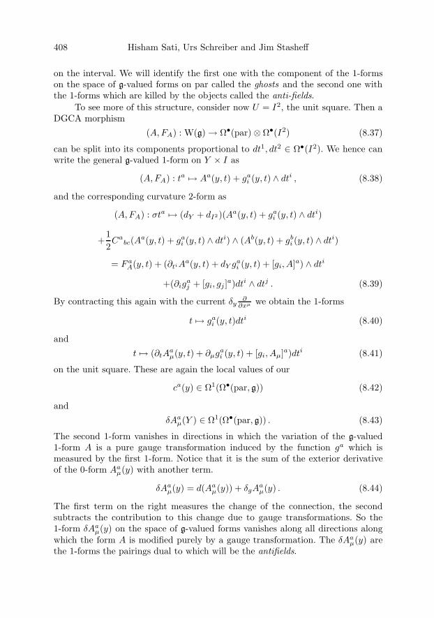
408 Hisham Sati, Urs Schreiber and Jim Stasheff
on the interval. We will identify the first one with the component of the 1-formson the space of g-valued forms on par called the ghosts and the second one withthe 1-forms which are killed by the objects called the anti-fields.
To see more of this structure, consider now U = I2, the unit square. Then aDGCA morphism
(A,FA) : W(g) → Ω•(par)⊗ Ω•(I2) (8.37)
can be split into its components proportional to dt1, dt2 ∈ Ω•(I2). We hence canwrite the general g-valued 1-form on Y × I as
(A,FA) : ta �→ Aa(y, t) + gai (y, t) ∧ dti , (8.38)
and the corresponding curvature 2-form as
(A,FA) : σta �→ (dY + dI2)(Aa(y, t) + gai (y, t) ∧ dti)
+12Ca
bc(Aa(y, t) + gai (y, t) ∧ dti) ∧ (Ab(y, t) + gb
i (y, t) ∧ dti)
= F aA(y, t) + (∂tiAa(y, t) + dY ga
i (y, t) + [gi, A]a) ∧ dti
+(∂igaj + [gi, gj ]a)dti ∧ dtj . (8.39)
By contracting this again with the current δy∂
∂xμ we obtain the 1-forms
t �→ gai (y, t)dti (8.40)
and
t �→ (∂tAaμ(y, t) + ∂μg
ai (y, t) + [gi, Aμ]a)dti (8.41)
on the unit square. These are again the local values of our
ca(y) ∈ Ω1(Ω•(par, g)) (8.42)
and
δAaμ(Y ) ∈ Ω1(Ω•(par, g)) . (8.43)
The second 1-form vanishes in directions in which the variation of the g-valued1-form A is a pure gauge transformation induced by the function ga which ismeasured by the first 1-form. Notice that it is the sum of the exterior derivativeof the 0-form Aa
μ(y) with another term.
δAaμ(y) = d(Aa
μ(y)) + δgAaμ(y) . (8.44)
The first term on the right measures the change of the connection, the secondsubtracts the contribution to this change due to gauge transformations. So the1-form δAa
μ(y) on the space of g-valued forms vanishes along all directions alongwhich the form A is modified purely by a gauge transformation. The δAa
μ(y) arethe 1-forms the pairings dual to which will be the antifields.

L∞-Algebra Connections and Applications 409
2-Forms. We have already seen the 2-form appear on the standard square. We callthis 2-form
βa ∈ Ω2(Ω•(par, g)) , (8.45)
corresponding on the unit square to the assignment
βa : (Ω•(par× I2) ← W(g) : A) �→ (∂igaj + [gi, gj]a)dti ∧ dtj . (8.46)
There is also a 2-form coming from (σta)δy. Then one immediately sees that ourforms on the space of g-valued forms satisfy the relations
dca(y) = −12Ca
bccb(y) ∧ cc(y) + βa(y) (8.47)
dβa(y) = −Cabcc
b(y) ∧ βc(y) . (8.48)
The 2-form β on the space of g-valued forms is what is being contracted by thehorizontal pairings called the antighosts. We see, in total, that Ω•(Ω•(par, g)) isthe Weil algebra of a DGCA, which is obtained from the above formulas by settingβ = 0 and δA = 0. This DGCA is the algebra of the gauge groupoid, that wherethe only morphisms present are gauge transformations.
The computation we have just performed are over U = I2. However, it shouldbe clear how this extends to the general case.
Chern-Simons theory. One can distinguish two ways to set up Chern-Simons the-ory. In one approach one regards principal G-bundles on abstract 3-manifolds, inthe other approach one fixes a given principal G-bundle P → X on some basespace X , and pulls it back to 3-manifolds equipped with a map into X . Physically,the former case is thought of as Chern-Simons theory proper, while the latter casearises as the gauge coupling part of the membrane propagating on X . One tendsto want to regard the first case as a special case of the second, obtained by lettingX = BG be the classifying space for G-bundles and P the universal G-bundle onthat.
In our context this is realized by proposition 6.14, which gives the canonicalChern-Simons 3-bundle on BG in terms of a b2u(1)-connection descent object onW(g). Picking some 3-dimensional parameter space manifold par, we can transgressthis b2u(1)-connection to the configuration space maps(W(g),Ω•(par)), which we
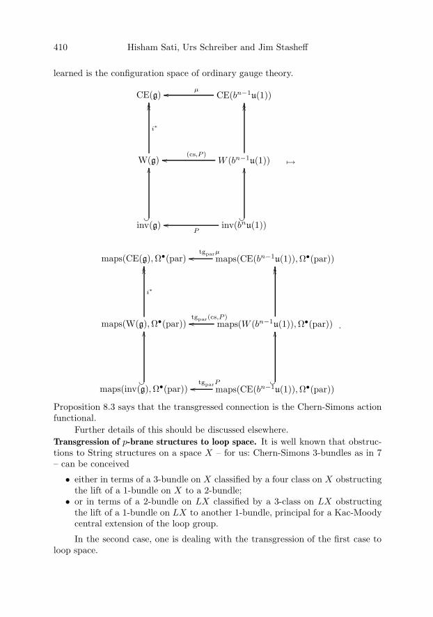
410 Hisham Sati, Urs Schreiber and Jim Stasheff
learned is the configuration space of ordinary gauge theory.
CE(g) CE(bn−1u(1))μ��
W(g)
i∗
����
W (bn−1u(1))
����
(cs,P )��
inv(g)��
��
inv(bnu(1))��
��
P��
�→
maps(CE(g),Ω•(par) maps(CE(bn−1u(1)),Ω•(par))tgparμ��
maps(W(g),Ω•(par))
i∗
����
maps(W (bn−1u(1)),Ω•(par))
����
tgpar(cs,P )��
maps(inv(g),ٕ(par))��
��
maps(CE(bn−1u(1)),Ω•(par))��
��
tgparP��
.
Proposition 8.3 says that the transgressed connection is the Chern-Simons actionfunctional.
Further details of this should be discussed elsewhere.Transgression of p-brane structures to loop space. It is well known that obstruc-tions to String structures on a space X – for us: Chern-Simons 3-bundles as in 7– can be conceived
• either in terms of a 3-bundle on X classified by a four class on X obstructingthe lift of a 1-bundle on X to a 2-bundle;
• or in terms of a 2-bundle on LX classified by a 3-class on LX obstructingthe lift of a 1-bundle on LX to another 1-bundle, principal for a Kac-Moodycentral extension of the loop group.
In the second case, one is dealing with the transgression of the first case toloop space.

L∞-Algebra Connections and Applications 411
The relation between the two points of views is carefully described in [56].Essentially, the result is that rationally both obstructions are equivalent.
Remark. Unfortunately, there is no universal agreement on the convention of thedirection of the operation called transgression. Both possible conventions are usedin the literature relevant for our purpose here. For instance [18] say transgressionfor what [2] calls the inverse of transgression (which, in turn, should be calledsuspension).
We will demonstrate in the context of L∞-algebra connections how Lie al-gebra (n + 1)-cocycles related to p-brane structures on X transgress to loop Liealgebra n-cocycles on loop space. One can understand this also as an alternativeproof of the strictification theorem of the String Lie 2-algebra (proposition 5.35),but this will not be further discussed here.
So let g be an ordinary Lie algebra, μ an (n + 1)-cocycle on it in transgres-sion with an invariant polynomial P , where the transgression is mediated by thetransgression element cs as described in section 5.3.
According to proposition 6.14 the corresponding universal obstruction struc-ture is the bnu(1)-connection
CE(g) CE(bnu(1))�
W(g)
����
W(bnu(1))(cs,P )��
����
inv(g)� �
��
inv(bnu(1)) = CE(bn+1u(1)){P}��
� �
�� (8.49)
to be thought of as the universal higher Chern-Simons (n + 1)-bundle with con-nection on the classifying space of the simply connected Lie group integratingg.
We transgress this to loops by applying the functor maps(−,Ω•(S1)) fromdefinition 4.4 to it, which can be thought of as computing for all DGC algebrasthe DGC algebra of differential forms on the space of maps from the circle into
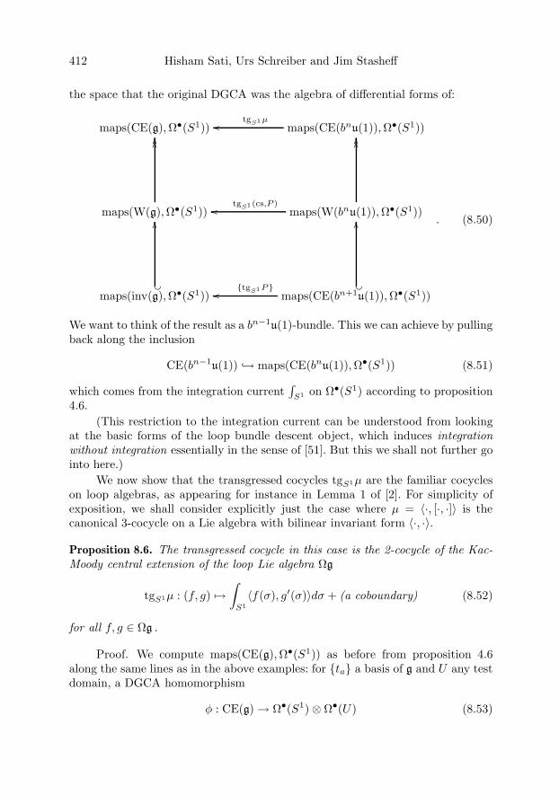
412 Hisham Sati, Urs Schreiber and Jim Stasheff
the space that the original DGCA was the algebra of differential forms of:
maps(CE(g),ٕ(S1)) maps(CE(bnu(1)),ٕ(S1))tgS1�
maps(W(g),Ω•(S1))
����
maps(W(bnu(1)),ٕ(S1))tgS1(cs,P )��
����
maps(inv(g),Ω•(S1))� �
��
maps(CE(bn+1u(1)),ٕ(S1)){tgS1P}��
� �
�� . (8.50)
We want to think of the result as a bn−1u(1)-bundle. This we can achieve by pullingback along the inclusion
CE(bn−1u(1)) ↪→ maps(CE(bnu(1)),Ω•(S1)) (8.51)
which comes from the integration current∫
S1 on Ω•(S1) according to proposition4.6.
(This restriction to the integration current can be understood from lookingat the basic forms of the loop bundle descent object, which induces integrationwithout integration essentially in the sense of [51]. But this we shall not further gointo here.)
We now show that the transgressed cocycles tgS1μ are the familiar cocycleson loop algebras, as appearing for instance in Lemma 1 of [2]. For simplicity ofexposition, we shall consider explicitly just the case where μ = 〈·, [·, ·]〉 is thecanonical 3-cocycle on a Lie algebra with bilinear invariant form 〈·, ·〉.
Proposition 8.6. The transgressed cocycle in this case is the 2-cocycle of the Kac-Moody central extension of the loop Lie algebra Ωg
tgS1μ : (f, g) �→∫
S1〈f(σ), g′(σ)〉dσ + (a coboundary) (8.52)
for all f, g ∈ Ωg .
Proof. We compute maps(CE(g),Ω•(S1)) as before from proposition 4.6along the same lines as in the above examples: for {ta} a basis of g and U any testdomain, a DGCA homomorphism
φ : CE(g) → Ω•(S1)⊗ Ω•(U) (8.53)

L∞-Algebra Connections and Applications 413
sends
ta� φ ��
�
dCE(g)
��
ca + Aaθ�
dS1+dU
��
− 12C
abct
b ∧ tc� φ �� θ∧( ∂
∂σ ca)+dUca+dU Aa∧θ
=− 12 Ca
bccb∧cc−Cabccb∧Ab∧θ
. (8.54)
Here θ ∈ Ω1(S1) is the canonical 1-form on S1 and ∂∂σ the canonical vector field;
moreover ca ∈ Ω0(S1)⊗ Ω1(U) and Aaθ ∈ Ω1(S1)⊗ Ω0(U).By contracting with δ-currents on S1 we get 1-forms ca(σ), ∂
∂σ ca(σ) and
0-forms Aa(σ) for all σ ∈ S1 on maps(CE(g),Ω•(S1)) satisfying
dmaps(··· )ca(σ) +12Ca
bccb(σ) ∧ cc(σ) = 0 (8.55)
and
dmaps(··· )Aa(σ)− CabcA
b(σ) ∧ cc(σ) =∂
∂σca(σ) . (8.56)
Notice the last term appearing here, which is the crucial one responsible for theappearance of derivatives in the loop cocycles, as we will see now.
So Aa(σ) (a “field”) is the function on (necessarily flat) g-valued 1-forms onS1 which sends each such 1-form for its ta-component along θ at σ, while ca(σ) (a“ghost”) is the 1-form which sends each tangent vector field to the space of flatg-valued forms to the gauge transformation in ta direction which it induces on thegiven 1-form at σ ∈ S1.
Notice that the transgression of our 3-cocycle
μ = μabcta ∧ tb ∧ tc = Cabct
a ∧ tb ∧ tc ∈ H3(CE(g)) (8.57)
is
tgS1μ =∫
S1CabcA
a(σ)cb(σ) ∧ cc(σ) dσ ∈ Ω2(Ω1flat(S
1, g) . (8.58)
We can rewrite this using the identity
dmaps(··· )
(∫S1
PabAa(σ)cb(σ)dσ
)=
∫S1
Pab (∂σca(σ)) ∧ cb(σ)
+12
∫S1
CabcAa(σ)cb(σ) ∧ cc(σ),(8.59)
which follows from 8.55 and 8.56, as
tgS1μ =∫
S1Pab (∂σc
a(σ)) ∧ cb(σ) + dmaps(··· )(· · · ) . (8.60)
Then notice that• equation (8.55) is the Chevalley-Eilenberg algebra of the loop algebra Ωg;
414 Hisham Sati, Urs Schreiber and Jim Stasheff
• the term∫
S1 Pab(∂σca(σ))∧cb(σ) is the familiar 2-cocycle on the loop algebra
obtained from transgression of the 3-cocycle μ = μabcta ∧ tb ∧ tc = Cabct
a ∧tb ∧ tc .
�
9. Physical applications: string-, fivebrane- and p-brane structures
We can now discuss physical applications of the formalism that we have developed.What we describe is a useful way to handle obstructing n-bundles of various kindsthat appear in string theory. In particular, we can describe generalizations of stringstructure in string theory. In the context of p-branes, such generalizations havebeen suggested based on p-loop spaces [30] [10] [64] and, more generally, on thespace of maps Map(M,X) from the brane worldvolume M to spacetime X [60].The statements in this section will be established in detail in [68].
From the point of view of supergravity, all branes, called p-branes in thatsetting, are a priori treated in a unified way. In tracing back to string theory, how-ever, there is a distinction in the form-fields between the Ramond-Ramond (RR)and the Neveu-Schwarz (NS) forms. The former live in generalized cohomologyand the latter play two roles: they act as twist fields for the RR fields and they arealso connected to the geometry and topology of spacetime. The H-field H3 playsthe role of a twist in K-theory for the RR fields [50] [15] [59]. The twist for thedegree seven dual field H7 is observed in [67] at the rational level.
The ability to define fields and their corresponding partition functions putsconstraints on the topology of the underlying spacetime. The most commonly un-derstood example is that of fermions where the ability to define them requiresspacetime to be spin, and the ability to describe theories with chiral fermionsrequires certain restrictions coming from the index theorem. In the context of het-erotic string theory, the Green-Schwarz anomaly cancelation leads to the conditionthat the difference between the Pontrjagin classes of the tangent bundle and that ofthe gauge bundle be zero. This is called the string structure, which can be thoughtof as a spin structure on the loop space of spacetime [52] [27]. In M-theory, theability to define the partition function leads to an anomaly given by the integralseventh-integral Stiefel-Whitney class of spacetime [29] whose cancelation requiresspacetime to be orientable with respect to generalized cohomology theories beyondK-theory [55] .
In all cases, the corresponding structure is related to the homotopy groupsof the orthogonal group: the spin structure amounts to killing the first homotopygroup, the string structure and – to some extent– the W7 condition to killing thethird homotopy group. Note that when we say that the n-th homotopy group iskilled, we really mean that all homotopy groups up to and including the n-th

L∞-Algebra Connections and Applications 415
one are killed. For instance, a String structure requires killing everything up toand including the third, hence everything through the sixth, since there are nohomotopy groups in degrees four, five or six.
The Green-Schwarz anomaly cancelation condition for the heterotic stringcan be translated to the language of n-bundles as follows. We have two bundles,the spin bundle with structure group G = Spin(10), and the gauge bundle withstructure group G′ being either SO(32)/Z2 or E8×E8. Considering the latter, wehave one copy of E8 on each ten-dimensional boundary component, which can beviewed as an end-of-the-world nine-brane, or M9-brane [47]. The structure of thefour-form on the boundary which we write as
G4|∂ = dH3 (9.1)
implies that the 3-bundle (2-gerbe) becomes the trivializable lifting 2-gerbe of aString(Spin(10) × E8) bundle over the M9-brane. As the four-form contains thedifference of the Pontrjagin classes of the bundles with structure groups G andG′, the corresponding three-form will be a difference of Chern-Simons forms. Thebundle aspect of this has been studied in [12] and will be revisited in the currentcontext in [68].
The NS fields play a special role in relation to the homotopy groups of theorthogonal group. The degree three class [H3] plays the role of a twist for a spinstructure. Likewise, the degree seven class plays a role of a twist for a higherstructure related to BO〈9〉, the 8-connected cover of BO, which we might call aFivebrane-structure on spacetime. We can talk about such a structure once thespacetime already has a string structure. The obstructions are given in table 4,where A is the connection on the G′ bundle and ω is a connection on the G bundle.
n2
= 4 · 0 + 26
= 4 · 1 + 2fundamental object
(n− 1)-branen-particle
string 5-brane
target spacestructure
string structurech2(A)− p1(ω) = 0
fivebrane structurech4(A)− 1
48p2(ω) = 0
Table 4. Higher dimensional extended objects and the corre-sponding topological structures.
In the above we alluded to how the brane structures are related to obstruc-tions to having spacetimes with connected covers of the orthogonal groups asstructures. The obstructing classes here may be regarded as classifying the corre-sponding obstructing n-bundles, after we apply the general formalism that we out-lined earlier. The main example of this general mechanism that will be of interest

416 Hisham Sati, Urs Schreiber and Jim Stasheff
to us here is the case where g is an ordinary semisimple Lie algebra. In particular,we consider g = spin(n). For g = spin(d) and μ a (2n + 1)-cocycle on spin(d), wecall spin(d)μ the (skeletal version of the) (2n− 1)-brane Lie (2n)− algebra. Thus,the case of String structure and Fivebrane structure occurring in the fundamentalstring and NS fivebrane correspond to the cases n = 1 and n = 3 respectively. Nowapplying our formalism for g = spin(d), and μ3, μ7 the canonical 3- and 7-cocycle,respectively, we have:• the obstruction to lifting a g-bundle descent object to a String 2-bundle (a
gμ3 -bundle descent object) is the first Pontryagin class of the original g-bundlecocycle;
• the obstruction to lifting a String 2-bundle descent object to a Fivebrane 6-bundle cocycle (a gμ7 -bundle descent object) is the second Pontryagin classof the original g-bundle cocycle.The cocyles and invariant polynomials corresponding to the two structures
are given in the following table
p-brane cocycle invariantpolynomial
p = 1 = 4 · 0 + 1 μ3 = 〈·, [·, ·]〉 P1 = 〈·, ·〉 first Pontrjaginp = 5 = 4 · 1 + 1 μ7 = 〈·, [·, ·], [·, ·], [·, ·]〉 P2 = 〈·, ·, ·, ·〉 second Pontrjagin
Table 5. Lie algebra cohomology governing NS p-branes.
In case of the fundamental string, the obstruction to lifting the PU(H) bun-dles to U(H) bundles is measured by a gerbe or a line 2-bundle. In the language ofE8 bundles this corresponds to lifting the loop group LE8 bundles to the centralextension LE8 bundles [59]. The obstruction for the case of the String structureis a 2-gerbe and that of a Fivebrane structure is a 6-gerbe. The structures aresummarized in the following table
obstruction → G-bundle ⇒ G-bundle1-gerbes / line 2-bundles2-gerbes / line 3-bundles6-gerbes / line 7-bundles
→PU(H)-bundlesSpin(n)-bundles
String(n)-2-bundles⇒
U(H)-bundlesString(n)-2-bundles
FiveBrane(n)-6-bundles
Table 6. Obstructing line n-bundles appearing in string theory,where→ equals the phrase “obstruct the lift of”, and⇒ equals the phrase “to”.
A description can also be given in terms of (higher) loop spaces, generalizingthe known case where a String structure on a space X can be viewed as a Spinstructure on the loop space LX . A fuller discussion of the ideas of this section isgiven in [68] and [69].
L∞-Algebra Connections and Applications 417
Appendix A. Explicit formulas for 2-morphisms of L∞-algebras
To the best of our knowledge, the only place in the literature where 2-morphismsbetween 1-morphisms of L∞-algebras have been spelled out in detail is [5], whichgives a definition of 2-morphisms for Lie 2-algebras, i.e. for L∞-algebras concen-trated in the lowest two degrees. Our definition 5.11 provides an algorithm forcomputing 2-morphisms between morphisms of arbitrary (finite dimensional) L∞-algebras. We had already demonstrated in 5.2 one application of that algorithm,showing explicitly how it allows to compute transgression elements (Chern-Simonsforms).
For completeness, we demonstrate that the formulas given in [5] for the specialcase of Lie 2-algebras also follow as a special case from our general definition5.11. This is of relevance to our discussion of the String Lie 2-algebra, since theequivalence of its strict version with its weak skeletal version, mentioned in ourproposition 5.35, has been established in [7] using these very formulas. First wequickly recall the relevant definitions from [5, 7]: A “2-term” L∞-algebra is anL∞-algebra concentrated in the lowest two degrees. A morphism
ϕ : g → h (A.1)
of 2-term L∞-algebras g and h is a pair of maps
φ0 : g1 → h1 (A.2)φ1 : g2 → h2 (A.3)
together with a skew-symmetric map
φ2 : g1 ⊗ g1 → h2 (A.4)
satisfying
φ0(d(h)) = d(φ1(h)) (A.5)
as well as
d(φ2(x, y)) = φ0(l2(x, y))− l2(φ0(x), φ0(y)) (A.6)φ2(x, dh) = φ1(l2(x, h))− l2(φ0(x), φ1(h)) (A.7)
and finally
l3(φ0(x), φ0(y), φ0(z))− φ1(l3(x, y, z)) = φ2(x, l2(y, z)) + φ2(y, l2(z, x))+φ2(z, l2(x, y)) + l2(φ0(x), φ2(y, z)) + l2(φ0(y), φ2(z, x)) + l2(φ0(z), φ2(x, y)) .
for all x, y, z ∈ g1 and h ∈ g2. This follows directly from the requirement thatmorphisms of L∞-algebras be homomorphisms of the corresponding codifferentialcoalgebras, according to definition 5.2. The not quite so obvious aspect are theanalogous formulas for 2-morphisms:
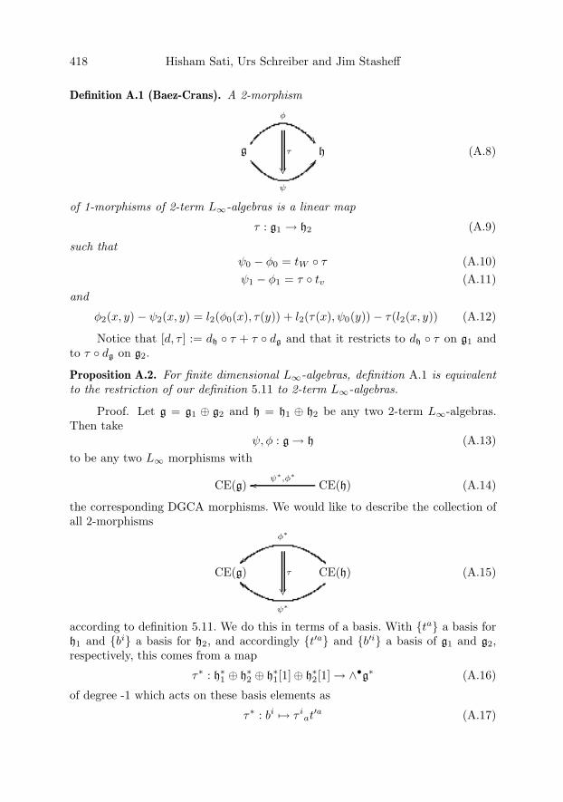
418 Hisham Sati, Urs Schreiber and Jim Stasheff
Definition A.1 (Baez-Crans). A 2-morphism
g
φ
23
ψ
34 hτ
(A.8)
of 1-morphisms of 2-term L∞-algebras is a linear map
τ : g1 → h2 (A.9)
such thatψ0 − φ0 = tW ◦ τ (A.10)ψ1 − φ1 = τ ◦ tv (A.11)
and
φ2(x, y)− ψ2(x, y) = l2(φ0(x), τ(y)) + l2(τ(x), ψ0(y))− τ(l2(x, y)) (A.12)
Notice that [d, τ ] := dh ◦ τ + τ ◦ dg and that it restricts to dh ◦ τ on g1 andto τ ◦ dg on g2.
Proposition A.2. For finite dimensional L∞-algebras, definition A.1 is equivalentto the restriction of our definition 5.11 to 2-term L∞-algebras.
Proof. Let g = g1 ⊕ g2 and h = h1 ⊕ h2 be any two 2-term L∞-algebras.Then take
ψ, φ : g → h (A.13)to be any two L∞ morphisms with
CE(g) CE(h)ψ∗,φ∗
�� (A.14)
the corresponding DGCA morphisms. We would like to describe the collection ofall 2-morphisms
CE(g) CE(h)
φ∗
ψ∗
��τ
(A.15)
according to definition 5.11. We do this in terms of a basis. With {ta} a basis forh1 and {bi} a basis for h2, and accordingly {t′a} and {b′i} a basis of g1 and g2,respectively, this comes from a map
τ∗ : h∗1 ⊕ h∗2 ⊕ h∗1[1]⊕ h∗2[1] → ∧•g∗ (A.16)
of degree -1 which acts on these basis elements as
τ∗ : bi �→ τ iat
′a (A.17)

L∞-Algebra Connections and Applications 419
andτ∗ : aa �→ 0 (A.18)
for some coefficients {τ ia}. Now the crucial requirement (5.65) of definition 5.11
is that (5.64) vanishes when restricted
CE(h)φ∗
��CE(g) W(h)
����
������������
�h∗[1]� ���
CE(h)ψ∗
��
� ������������
������������
(A.19)
to generators in the shifted copy of the Weil algebra. This implies the following. Forτ∗ to vanish on all σta we find that its value on dW(h)t
a = − 12C
abct
a∧tb−taibi+σta
is fixed to beτ∗ : dW(g)t
a �→ −taiτibt
′b (A.20)and on dW(h)b
i = −αiajt
a ∧ bj + ci to be
τ∗(dbi) = τ∗(−αiajt
a ∧ bj) . (A.21)
The last expression needs to be carefully evaluated using formula (5.61). Doing sowe get
[d, τ∗] : ta �→ −taiτibt
′b (A.22)and
[d, τ∗] : bi �→ −12τ i
aC′a
bct′bt′c − τ i
at′a
jb′j + αi
aj12(φ + ψ)a
bτjct
′bt′c . (A.23)
Then the expressionφ∗ − ψ∗ = [d, τ∗] (A.24)
is equivalent to the following ones
(ψab − φa
b)t′b = taiτibt
′b (A.25)
(ψij − φi
j)b′j = τ iat
′ajb
′j (A.26)12(φi
ab − ψiab)t′at′b = −1
2τ i
aC′a
bct′bt′c + αi
aj12(φ + ψ)a
bτjct
′bt′c .(A.27)
The first two equations express the fact that τ is a chain homotopy with respectto t and t′. The last equation is equivalent to
φ2(x, y)− ψ2(x, y) = −τ([x, y]) + [q(x) +12t(τ(x)), τ(y)]
−[q′(y)− 12t(τ(y)), τ(x)]
= −τ([x, y]) + [q(x), τ(y)] + [τ(x), q′(y)] (A.28)
This is indeed the Baez-Crans condition on a 2-morphism. �
420 Hisham Sati, Urs Schreiber and Jim Stasheff
Acknowledgements
We thank Danny Stevenson for many helpful comments. Among other things, thediscussion of the cohomology of the string Lie 2-algebra has been greatly influencedby conversation with him. We acknowledge stimulating remarks by John Baez oncharacteristic classes of string bundles. H.S. thanks Matthew Ando and U.S. thanksStephan Stolz and Peter Teichner for discussions at an early stage of this work.
U.S. thankfully acknowledges invitations to the University of Oxford by NigelHitchin; to the conference “Lie algebroids and Lie groupoids in differential geome-try” in Sheffield by Kirill Mackenzie and Ieke Moerdijk; to the Erwin SchrodingerInstitute in the context of the program “Poisson σ-models, Lie algebroids, defor-mations and higher analogues”; to “Categories in Geometry and Physics” by ZoranSkoda and Igor Bakovic; and to Yale University which led to collaboration withH.S. and to useful discussions with Mikhail Kapranov. U.S. thanks Todd Trimblefor discussion of DGCAs, and their relation to smooth spaces, thanks MathieuDupont and Larry Breen for discussion about weak cokernels and thanks SimonWillerton and Bruce Bartlett for helpful discussion of the notion of transgression.H.S. thanks Akira Asada and Katsuhiko Kuribayashi for useful correspondence ontheir work on (higher) string structures.
We thank the contributors to the weblog The n-Category Cafe for much inter-esting, often very helpful and sometimes outright invaluable discussion concerningthe ideas presented here and plenty of related issues.
We have gratefully received useful comments on earlier versions of this doc-ument from Gregory Ginot and David Roberts. Evan Jenkins and Todd Trimblehave provided useful help with references to literature on smooth function algebras.
While this article was being written, the preprints [80], [54] and [36] (basedon [37]) appeared, which are closely related to our discussion here in that theyaddress the issues of characteristic classes and extensions of n-bundles in one wayor another. We are thankful to Amnon Yekutieli and to Gregory Ginot for pointingout their work to us and for further discussion.
Finally, we thank Bertfried Fauser and the organizers of the conference “Re-cent developments in QFT” in Leipzig.
U.S. thankfully acknowledges financial support from the DAAD German-Croatian bilateral project “Nonabelian cohomology and applications”.
References
[1] M. Alexandrov, M. Kontsevich, A. Schwarz and O. Zaboronsky, The Ge-ometry of the Master Equation and Topological Quantum Field Theory,[http://arxiv.org/refs/hep-th/0608150]
[2] A. Asada, Characteristic classes of loop group bundles and generalized stringclasses, Differential geometry and its applications (Eger, 1989), 33-66, Colloq.Math. Soc. Janos Bolyai, 56, North-Holland, Amsterdam, (1992)
L∞-Algebra Connections and Applications 421
[3] P. Aschieri and B. Jurco, Gerbes, M5-brane anomalies and E8 gauge theory J.High Energy Phys. 0410 (2004) 068, [arXiv:hep-th/0409200v1].
[4] R. D’Auria and P. Fre, Geometric supergravity in D = 11 and its hidden super-group, Nuclear Physics B, 201 (1982)
[5] J. Baez and A. Crans, Higher-dimensional algebra VI: Lie 2-algebras, Theory andApplications of Categories 12 (2004) 492–528, [arXiv:math/0307263v5].
[6] T. Bartels, 2-Bundles, [arXiv:math/0410328v3]
[7] J. Baez, A. Crans, U. Schreiber and D. Stevenson, From Loop Groups to 2-Groups, Homology, Homotopy and Applications, Vol. 9 (2007), No. 2, pp.101–135,[arXiv:math/0504123v2].
[8] J. Baez and D. Stevenson, The Classifying Space of a Topological 2-Group,[arXiv:0801.3843v1]
[9] J. Baez and U. Schreiber, Higher gauge theory, in Contemporary Math-ematics, 431, Categories in Algebra, Geometry and Mathematical Physics,[arXiv:math/0511710].
[10] E. Bergshoeff, R. Percacci, E. Sezgin, K.S. Stelle, and P.K. Townsend, U(1)-extended gauge algebras in p-loop space, Nucl. Phys. B 398 (1993) 343,[arXiv:hep-th/9212037v1].
[11] E. Bergshoeff, E. Sezgin, and P.K. Townsend, Properties of the eleven-dimensionalsuper membrane theory, Annals Phys.185 (1988) 330.
[12] L. Bonora, P. Cotta-Ramusino, M. Rinaldi, and J. Stasheff, The evaluation mapin field theory, sigma-models and strings I, Commun. Math. Phys. 112 (1987) 237.
[13] A. Borel, Sur la cohomologie des espaces fibres principaux et des espaces homognesde groupes de Lie compacts, Ann. Math. (2) 57 (1953), 115–207.
[14] A.K. Bousfield and V.K.A.M. Gugenheim, On PL de Rham theory and rationalhomotopy type, Mem. Amer. Math. Soc.8 (1976), no. 179.
[15] P. Bouwknegt and V. Mathai, D-branes, B-fields and twisted K-theory, J. HighEnergy Phys. 03 (2000) 007, [arXiv:hep-th/0002023].
[16] P. Bouwknegt, A. Carey, V. Mathai, M. Murray and D. Stevenson, Twisted K-theory and K-theory of bundle gerbes, Commun. Math. Phys. 228 (2002) 17,[arXiv:hep-th/0106194].
[17] L. Breen and W. Messing, Differential geometry of gerbes, Adv. Math. 198 (2005),no. 2, 732–846, [arXiv:math/0106083v3].
[18] J.-L. Brylinski and D.A. McLaughlin, Cech cocycles for characteristic classes,Comm. Math. Phys. 178, 225–236 (1996)
[19] J.-L. Brylinski and D.A. McLaughlin, A geometric construction of the first Pon-tryagin class, Quantum Topology, 209-220, World Scientific (1993)
[20] A. Carey, S. Johnson, and M. Murray, Holonomy on D-branes, J. Geom. Phys. 52(2004), no. 2, 186–216, [arXiv:hep-th/0204199v3].
[21] A. Carey, S. Johnson, M. Murray, D. Stevenson, and B.-L. Wang, Bundle gerbesfor Chern-Simons and Wess-Zumino-Witten theories , Commun. Math. Phys. 259(2005) 577, [arXiv:math/0410013].
422 Hisham Sati, Urs Schreiber and Jim Stasheff
[22] H. Cartan, Notions d’algebre differentielle; application aux groupes de Lie et auxvarietes ou opere un groupe de Lie, Colloque de topologie (espaces fibrs), Bruxelles,1950, pp. 15–27.
[23] H. Cartan, Cohomologie reelle d’un espace fibre principal diffrentielle I, II,Seminaire Henri Cartan, 1949/50, pp. 19-01 – 19-10 and 20-01 – 20-11, CBRM,1950.
[24] L. Castellani, R. D’Auria and P. Fre, Supergravity and superstrings: a geometricperspective, World Scientific, Singapore (1991)
[25] J. Cheeger and J. Simons, Differential characters and geometric invariants, inGeometry and Topology, 50–80, Lecture Notes in Math., 1167, Springer-Verlag,1985.
[26] A. Clingher, Heterotic string data and theta functions, Adv. Theor. Math. Phys.9 (2005) 173, [arXiv:math/0110320v2].
[27] R. Coquereaux and K. Pilch, String structures on loop bundles, Commun. Math.Phys. 120 (1989) 353.
[28] E. Diaconescu, D. Freed, and G. Moore, The M theory three form and E8 gaugetheory,[arXiv:hep-th/0312069].
[29] E. Diaconescu, G. Moore and E. Witten, E8 gauge theory, and a deriva-tion of K-theory from M-theory Adv. Theor. Math. Phys. 6 (2003) 1031,[arXiv:hep-th/0005090].
[30] J.A. Dixon, M.J. Duff, and E. Sezgin, The coupling of Yang-Mills to extendedobjects, Phys. Lett. B 279 (1992) 265, [arXiv:hep-th/9201019v1].
[31] D.S. Freed, Classical Chern-Simons Theory, Part I, [hep-th/9206021v1]
[32] D.S. Freed, Higher algebraic structures and quantization,[arXiv:hep-th/9212115v2]
[33] D.S. Freed, Quantum groups from path integrals, [arXiv:q-alg/9501025v1]
[34] D.S. Freed and E. Witten, Anomalies in string theory with D-Branes, Asian J.Math. 3 (1999) 819, [arXiv:hep-th/9907189].
[35] E. Getzler, Lie theory for nilpotent L∞-algebras, Ann. Math.[arXiv:math/0404003v4]
[36] G. Ginot and M. Stienon, Groupoid extensions, principal 2-group bundles andcharacteristic classes, [arXiv:0801.1238v1].
[37] G. Ginot and P. Xu Cohomology of Lie 2-groups, [arXiv:0712.2069v1].
[38] F. Girelli and H. Pfeiffer, Higher gauge theory – differential versus integral formu-lation, J. Math. Phys. 45 (2004) 3949-3971, [arXiv:hep-th/0309173v2].
[39] F. Girelli, H. Pfeiffer, and E. Popescu, Topological higher gauge theory - from BFto BFCG theory, [arXiv:0708.3051v1].
[40] M.B. Green and J.H. Schwarz, Anomaly cancellation in supersymmetric D = 10gauge theory and superstring theory, Phys. Lett. B149 (1984) 117.
[41] W. Greub, S. Halperin, and R. Vanstone, Connections, curvature, and cohomology.Vol. II: Lie groups, principal bundles, and characteristic classes, Academic Press,New York-London, 1973.
L∞-Algebra Connections and Applications 423
[42] S. Halperin and J.-C. Thomas, Rational equivalence of fibrations with fibre G/K,Canad. J. Math. 34 (1982), no. 1, 31–43.
[43] A. Henriques, Integrating L∞ algebras, [arXiv:math/0603563v2].
[44] K. Hess, Rational Homotopy Theory: A Brief Introduction,[http://www.math.uic.edu/~bshipley/hess_ratlhtpy.pdf]
[45] M.J. Hopkins, Topological aspects of topological field theories, Andrejewski lecture,Gottingen (2006)
[46] M.J. Hopkins, I.M. Singer, Quadratic functions in geometry, topology, and M-theory, J. Diff. Geom. 70 (2005) 329-452, [arXiv:math.AT/0211216].
[47] P. Horava and E. Witten, Eleven-dimensional supergravity on a manifold withboundary, Nucl.Phys. B475 (1996) 94, [arXiv:hep-th/9603142].
[48] P.T. Johnstone, Stone Spaces, Cambridge studies in advanced mathematica (1986)
[49] J. Kalkman, BRST model for equivariant cohomology and representatives for theequivariant Thom class, Comm. Math. Phys. 153 (1993), no. 3, 447–463.
[50] A. Kapustin, D-branes in a topologically nontrivial B-field, Adv. Theor.Math. Phys. 4 (2000) 127, [arXiv:hep-th/9909089].
[51] L.H. Kauffman, Vassiliev invariants and functional integration without integration,in Stochastic analysis and mathematical physics, p 91-114
[52] T.P. Killingback, World-sheet anomalies and loop geometry, Nucl. Phys. B 288(1987) 578.
[53] I. Kolav r, J. Slova k and P.W. Michor, Natural operations in differential geometry,Springer-Verlag (1993)
[54] A. Kotov and Th. Strobl, Characteristic classes associated to Q-bundles,[arXiv:0711.4106v1]
[55] I. Kriz and H. Sati, M Theory, type IIA superstrings, and elliptic cohomology, Adv.Theor. Math. Phys. 8 (2004) 345, [arXiv:hep-th/0404013].
[56] K. Kuribayashi, On the vanishing problem of String classes, J. Austr. Math. Soc.(Series A) 61, 258-266 (1996)
[57] T. Lada and J. Stasheff, Introduction to sh Lie algebras for physicists, Int. J.Theor. Phys. 32 (1993) 1087, [arXiv:hep-th/9209099].
[58] T. Lada, M. Markl, Strongly homotopy Lie algebras, Comm. Algebra 23 (1995),no. 6, 2147–2161, [arXiv:hep-th/9406095v1].
[59] V. Mathai and H. Sati, Some relations between twisted K-theory and E8 gaugetheory, J. High Energy Phys. 0403 (2004) 016, [arXiv:hep-th/0312033v4].
[60] J. Mickelsson and R. Percacci, Global aspects of p-branes, J. Geom. and Phys. 15(1995) 369-380, [arXiv:hep-th/9304054v1].
[61] I. Moerdijk and G. Reyes, Models for smooth infinitesimal analysis, Springer-Verlag (1991)
[62] M. Murray, Bundle gerbes, J. London Math. Soc. (2) 54 (1996), no. 2, 403–416.
[63] M. Murray and D. Stevenson, Higgs fields, bundle gerbes and string structures,Commun. Math. Phys. 243 (2003) 541–555, [arXiv:math/0106179v1].
[64] R. Percacci and E. Sezgin, Symmetries of p-branes, Int. J. Theor. Phys. A 8 (1993)5367, [arXiv:hep-th/9210061v1].
424 Hisham Sati, Urs Schreiber and Jim Stasheff
[65] D. Roberts and U. Schreiber, The inner automorphism 3-group of a strict 2-group,to appear in Journal of Homotopy and Related Structures, [arXiv:0708.1741].
[66] D. Roytenberg, AKSZ-BV Formalism and Courant Algebroid-induced TopologicalField Theories, [http://arxiv.org/abs/hep-th/0608150]
[67] H. Sati, On Higher twists in string theory, [arXiv:hep-th/0701232v2 ].
[68] H. Sati, U. Schreiber, J. Stasheff Fivebrane structures: topology, [arXiv:0805.0564]
[69] H. Sati, U. Schreiber, J. Stasheff Fivebrane structures: geometry, (in preparation)
[70] U. Schreiber, On nonabelian differential cohomology, lecture notes,[http://www.math.uni-hamburg.de/home/schreiber/ndclecture.pdf]
[71] U. Schreiber, On ∞-Lie theory,[http://www.math.uni-hamburg.de/home/schreiber/action.pdf]
[72] U. Schreiber and K. Waldorf, Parallel transport and functors,[arXiv:0705.0452v1].
[73] U. Schreiber and K. Waldorf, 2-Functors vs. differential forms,[arXiv:0802.0663v1]
[74] U. Schreiber and K. Waldorf, Connections on non-abelian Gerbes and their Holo-nomy, to appear.
[75] J. Stasheff and M. Schlessinger, Deformation Theory and Rational Homotopy Type,unpublished.
[76] St. Stolz and P. Teichner, What is an elliptic object? in Topology, geometry andquantum field theory, London Math. Soc. LNS 308, Cambridge University Press2004, 247-343.
[77] Sullivan, Infinitesimal computations in topology , Publications mathematique de l
I.H.E.S., tome 47 (1977), p. 269–331
[78] C. Teitelboim and M. Henneaux, Quantization of gauge systems Princeton Uni-versity Press, 1992.
[79] E. Witten, On Flux quantization in M-Theory and the effective action, J. Geom.Phys. 22 (1997) 1–13, [arXiv:hep-th/9609122].
[80] A. Yekutieli, Central Extensions of Gerbes, [arXiv:0801.0083v1].
[81] T. Trimble, private communication
Hisham SatiDepartment of MathematicsYale University10 Hillhouse AvenueNew Haven, CT 06511e-mail: [email protected]
Jim StasheffDepartment of MathematicsUniversity of Pennsylvania209 South 33rd StreetPhiladelphia, PA 19104-6395e-mail: [email protected]
Urs SchreiberFachbereich MathematikUniversitat HamburgBundesstraße 55DE–20146 Hamburge-mail: [email protected]
Index
G-bundle
universal, 307
L∞-algebra
Chern-Simons, 356L∞-algebra, 303
2-term, 417
and differential forms, 309
Cartan-Ehresmann connection, 310
cohomology, 344
concordance, 338
definition, 306, 330from cocycles, 309, 355
homotopy, 338
normal subalgebra, 382
other names for, 306
parallel transport, 399
σ-model actions
from n-functorial parallel transport, 317n-bundle
with connection, 304
1-particle-irreducible diagrams, 184
2-morphism, 339
motivation
conceptual, 340practical, 340
of Lie 2-algebras, 344
Abrahamic heaven, 6
actionclassical, 50, 193
extended, 255
functional, 405
proper total, 193
AdS space
(anti de Sitter space), 68
Euclidean, 68half-space model of, 68
AdS/CFT
generating functional
alternative representation, 73
limiting functional, 73
AdS/CFT correspondence, 67
“German”, 20and string theory, 71
for models in statistical mechanics, 74
Airy integrals, 49
algebra
Chevalley-Eilenberg dg-, 331
of differential forms as DGCA, 318
single, as a structureless monad, 22
Weil, 336
Weil, as Lie 2-algebra, 334
Weil, of an L∞-algebra, 332algebraic renormalization
for non-expert readers, 194
recursiveness via the orders in �, 194
amplitude
renormalized, 141
anharmonic oscillator
effective equations for, 220
annihilation operatormass-shell, 2
anomalies
in loop quantum gravity, 232
anthropic principle, 18
anti de Sitter, see also AdS
approximation
adiabatic, 222semiclassical, 222
area density formula, 11
area law
for entropy localization, 10
for localization entropy, 22
of Bekenstein, 13
origin of, 4
Ashtekar connection, 219axioms of QFT
test of soundness of, 17
background field, 404
Barbero-Immirzi parameter, 219
Belavkin equation, 59β-function
of gravity, 160
of QED, 158
BF-term, 366
BF-theory, 317, 360, 366
functional, 402
interpreted as a Lie 2-algebragauge theory, 367
with cosmological term, 366Bianchi identity, 362
big bang
bounce, 228
bouncing solution, 229
singularity
classical, 226
Birkhoff decomposition, 146

426 Index
as renormalization, 146
for graded connected commutative Hopfalgebras, 147
Bogoliubov formula, 183
Boolean algebra
topological interpretation of, 28
Boolean topos, 28
Borel subgroup
of SU(3, C), 110
Born series
q-deformed, 280
boundary CFT
generating functional of, 75
boundary field
finite dimensional approximation of, 72
BPHZ-procedure, 141
BPHZ-renormalization
as Birkhoff decomposition, 147
brane
(n − 1)-, 404
higher dimensional, 304
BRST-field content, 406
Buddhist nirvana, 6
bundle
basic forms on a, 326
Caldeira-Legget model
for quantum Brownian motion, 59
Cartan’s magic formula, 324
Cartan-Ehresmann
condition, 368
condition, generalized, 374
connection, 310, 312, 367
ordinary, 375
category
context, 33
state object, 32
terminal object, 27
causal factorization, 183
causal perturbation theory, 178, 182
causal structure
discrete, definition of, 243
emergence of, 243
causality
in Minkowski space, 246
leakage, 14
central extension, 358
parameter, 11
CFT, see also conformal field theory
characteristic class, 315, 365, 376
as obstruction for String-like extension,396
invariance of, 365
characteristic function, 28
charged n-particle, 404
charges
conserved, 205
Chen’s iterated integral, 99
Chern class
first, 102
Chern-Simons
L∞-algebra, 356
n-transport, 312
2-gerbe, 305
3-bundle, 389
action functional, higher, 401
element, 340
generalized (n + 1)-bundle, 393
theory, 382, 409
vertical 3-form, as lifting obstruction, 389
Chevalley-Eilenberg algebra
of the loop algebra, 413
Chevalley-Eilenberg dg-algebra, 331
chiral field
transverse extended, 7
classical interaction, 186
classical physics
as a realist theory, 30
classical quantum transition asphase transition, 121
coarse-graining, 35
cocycle, 345
cohomological field theory
conjecture about, 90
cohomology, 350
Deligne, 370
in terms of qDGCAs, 349
of L∞-algebras, 344
of coset spaces, 390
commutant
as zeroth Hochschild cohomology, 130
commutation relations
for noncommutative coordinatefunctions, 118
plectonic (braid group), 8
concordance, 340
configuration space
of L∞-transport, 404
conformal boundary
for hyperbolic space, 69
conformal field theory
boundary conditions in, 68
conformal boundary, 68
conformal group action
Index 427
induced from AdS Lorentz transforma-tions, 69
conjecture
on the algebraic structure of cohomologi-cal field theory, 90
connection
Ashtekar, 219
Cartan-Ehresmann, 367
equivalence of g-, 374
extension problem for, 373
globally defined, 364
shift of, 371
spin, 219
variables, 218
conserved charges
“hidden”, 210
consistency equation
as a cocycle condition, 194
constraint
effective, 224
context category, 33, 34
of abelian von Neumann subalgebras, 25
continuum limit
in loop quantum gravity, 232
of the fermionic projector, 256
contractible
smoothly, 329
convolution
in momentum space, 248
coordinates
Brinkmann, 198, 202
Fermi, 203
Rosen, 198, 202
correlations
implemented by cumulants, 172
cosmological constant, 366
cosmological model
solvable, 225
counterterm, 141
boundary, 79
bulk, 79
coupling constant
dependent on the energy scale, 143
running, 143
covariance splitting formula, 69
Coxeter number
of SU(n), 107
creation operator
mass-shell, 2
critical manifold, 51
cross-ratio
conformal invariant, 12
current, 321
curvature, 361
3-, 367
4-form, 399
components β and H, 363
extrinsic, 219
of plane waves, 200
cut rule, 31
daseinisation
and Heidegger’s existential philosophy, 36
definition of, 36
inner and outer, 36
de Rham complex
vertical, 326
decoupling
for quadratic Hamiltonian, 222
deformation
equivalence of, 124
deformation quantization
definition of, 123
equivalence of, 127
existence of, 129
of a Hermitian fibre metric, 123
of a principal G-bundle, 126
degree of divergence, 156
degrees of freedom
cardinality of, 3
Deligne cohomology, 370
n-cocycle, 371
coboundary, 371
density matrix, 166
minimizing the energy, 171
derivation
inner, 323
encoding vector fields, 324
of L∞-algebras, 335
vertical, 324
derivative
Lie, 344
descent data
g-bundle, 368
descent object, 312
for g-connection, 373
in bijection with closed vertical n-forms,373
DGCA
(differential gradedcommutative algebra), 318
freeness of, 332
in non-positive degree, 321
mapping cone of, 332
428 Index
quasi free (≡ qDGCA), 321
diffeomorphism group
of the circle, 13
diffeomorphism invariance
generalized, 237
differential algebra
free, as qDGCA, 364
differential form
as DGCA, 319
basic, 348
on a smooth space, 319
differential forms, 318
differential graded commutativealgebra (DGCA), 318
differential operator
vertical, 130
Dirac sea, 246
with three generations, 256
discrete space-time, 235
fermion system, 237
divergence
cancellation of, 252
degree of, 156
Dixmier-Douady class, 350
Donaldson-Thaddeus-Witten
on SU(2) moduli space, 108
Dyson equation, 165
as generalized by Hall, 165
generalized, 169
Dyson-Schwinger equations
in QED4, 156
effective action
1-particle irreducible, 222
Ehrenfest theorem, 220
eigenstates
stationary, 207
Eilenberg-MacLane space, 309
Einstein, Albert
citation on the space-time continuum, 285
element
abstract notion of, 29
generalized, 29
global
of the presheaf of sieves, 43
horizontal, 380
of a category, 29
elliptic curves, 84
noncommutative, 83, 85
elliptic gamma function, 87
emergence
of causal structure, 243
of space-time, 258
energy
proportional to transverse area, 11
entanglement
entropy, 12
hot/cold, 7
intrinsic, 7
entropy
proportional to transverse area, 11
quantum, from Bekenstein’sinterpretation, 14
entropy localization
logarithmic divergence of, 11
Euclidean time, 72
Euler-Zagier multiple zeta functions, 98
existence proof
for QFT in 1 + 1 dimensions, 2
extension
central, 358
String-like, 309
properties of, 315
String-like, 315, 355, 356
obstructions to lifts, 316
weak cokernel in terms of theWeil algebra, 387
string-like
weak cokernel, 386
extensive quantity
transverse additivity of, 11
factorization property, 180
fc-multicategory, 90
fermion system
in discrete space-time, 237
fermionic projector, 236
discrete kernel, 238
regularization of, 252
state stable, 255
Feynman
on string theory, 21
Feynman diagram
1-particle irreducible, 184
generalized, 165
quantum part of a, 184
Feynman graph, 156
automorphism of, 144
definition of, 143
graded by loop number, 145
Hopf algebra for, 143
number of insertion points, 144
one-particle irreducible (1PI), 144
origin of, 139

Index 429
residue of, 144
Feynman path integral
approach to quantum mechanics, 50
convergence of using cancelation, 52
for the Schrodinger equation, 56
mathematical realization of, 52
not integrable in a Lebesgue sense, 53
Feynman rules
example amplitude, 140
for quantum electrodynamics (QED), 139
inducing an algebra map, 147
Feynman’s heuristic calculus
difficulties of, 51
Feynman-Vernon influence functional, 59
fiber bundle
as example of surjective submersions, 328
field
anti-, 405
field equation
off-shell, 182, 188
field independence, 183
filter, maximal, 42
Floer homology, 88
flow
vertical, 324
form
L∞-algebra valued, 361
g-valued, 361
flat, 361
basic, 327, 345
basic differential, 348
characteristic, 312, 376
curvature, 312
differential, 318
exmaples of, 362
invariant, 365
Neveu-Schwarz (NS), 414
Ramond-Ramond (RR), 414
formal language, 31
formfactor, multi-particle, 8
Fredholm determinant, 55
Fresnel integral, 49
Fukaya category
as a generalization, 89
deformation of, 88
functional integrals
on AdS, 68
functor
“maps”, 320
from smooth space to DGCA, 320
gamma function
elliptic, 86, 87
gauge
lightcone, 200
gauge coupling term, 399
gauge field
enveloping algebra valued, 132
gauge fixing, 142
gauge symmetry, 405
gauge theory, 141
fields of, 407
in the noncommutative framework, 125
gauge transformation, 370
as covariant transformation of curvature,340
Gauss linking number, 61
Gauss-Bonnet theorem, 160
Gaussian white noise measure, 56
Gel’fand spectrum, 33
as ‘local state space’, 26
Gel’fand transform, 34
Gell-Mann Low formula, 166
general relativity
linearized theory, 198
generating function
for free Green functions, 167
for Green function, 166
generator
coordinatizing, 3
Geodesics, 205
geodesics, 200
geometric Langlands correspondence, 84
gerbes
Abelian, 370
ghost
anti-, 405
Glaser-Lehmann-Zimmermann (GLZ)representation, 8
convergence status of, 9
gravity, 218
powercounting, 161
pure, 159
Green’s function, 139
diagrammatic expansion of, 168
for QED, 156
generating function of, 166
Hopf algebra of, 147
inverse of, 148
retarded, 180
Green-Schwarz
anomaly cancelation, 415
Gromov-Witten invariants
elliptic, definition of, 88

430 Index
noncommutative extension of, 84
group
and its function algebra, 266
Gutzwiller trace formula, 58
Haag, Rudolf, 2
Haag-Kastler theory, 2
Hagedorn temperature, 19
Hall’s equation
algebraic proof of, 170
Hamiltonian
effective, 171
harmonic oscillator, 206
time-dependent, 197
exact solution, 209
quadratic invariants, 211
Heisenberg algebra, 203
canonically normalized, 204
Heisenberg isometry algebra, 203
Hermitian fibre metric
as inner product, 123
Heyting algebra, 27
of subobjects, 38
Hirzebruch-Riemann-Roch formula, 97
Hochschild cohomology, 156
cochain, 128
holographic projection
of bulk fields, 5
of interacting pointlike bulk fields, 7
holography
algebraic, after Rehren, 15
algebraic, using operator algebras, 16
as a tool, 13
conceptual status of, 9
lightcone, 4
lightfront
gain of, 16
not a physical principle, 19
on null-surfaces, 4
projective, using Wightmann fields, 16
spirit of, 8
symmetry enhancement by, 13
holonomy, 399
Holy Grail
of a theory of everything, 2
HOMFLY polynomial, 60
homotopy
and inner derivations, 322
infinitesimal, 338
operator, 348
homotopy algebra
refered to as L∞-algebra, 306
homotopy group
related to string structure, 414
Hopf algebra, 152
antipode, 152
character, 146
coassociativity, 152
coproduct, 152
counit, 152
definition of a, 152
of Feynman graphs, 143
of Green’s functions, 147
Hopf fibration, 126
Hopf-Galois extension, 125
Hurwitz partition function, 85
hyperbolic space, 68
infra-red problem, 75
inner derivation, 323
encoding vector fields, 324
of L∞-algebras, 335
inner product
physical, 225
strongly non-degenerate, 123
insertion
in terms of R-products, 194
intellectual leader
role model of a, 20
interacting models
existence of, 22
interaction
classical, 186
gluon self-, 139
localized, 178
modified, 170
non localized, 178
of an exterior field, 75
photon with electron, 139
proper, 186
intersection pairing
computation of, 111
invariant charge, 158
invariant polynomial, 345
indecomposable, 350
lifted, closedness failure, 352
of bn−1u(1), 350
of String-like extensions, 357
suspened to 0, 358
IR problem, 67
Isham, Chris, 25
isometry algebra
Heisenberg, 203
solvable, 203

Index 431
iterated integral, 99
Jackson derivative, 270Jackson integral, 264
as operator, 271Jacobi
theta function, 87
triple product, 87Jacobi identity
q-deformed, 288Jones polynomial, 60Jordan, Pascual, 2
Kac-Weyl character formula, 104Kalb-Ramond field, 399Kauffman polynomial, 60
Keldysh formalism, 164Killing vector, 205
Kochen-Specker theorem, 26equivalent to element free presheaf, 34
Koszul sign, 330
Kripke-Joyal semantics, 38
Lagrangian
counter terms, 255lightcone gauge, 201
language
formal, 31representation of, in a topos, 32
latticedistributive, 27
lattice model
numerics, 257static and isotropic, 249
law of the excluded middle
not present in intuitionistic logic, 27legs
external, 156lengthscale
varying, 252
Leray-Hirsch theorem, 112Lewis-Riesenfeld procedure, 208
Lewis-Riesenfeld theory, 207Lie 2-algebra, 417
strict, 335
Lie 3-algebra, 360Lie 7-algebra, 360
Lie algebra, 331Lie derivative, 132, 324, 344lifting
obstruction to, 314lifting problem, 382
lightfront algebra
for interacting systems, 9
lightfront holography
for structural investigations, 10
line n-bundles
with equivalent connection, 371
linked cluster theorem, 185
Lippmann-Schwinger equation
q-deformed, 279
local correlation matrix, 241
logic
connectives “and”, “or”, “not”, 31
contextual, 25
cut rule, 31
intuitionistic, 27
quantifiers “it exists” and “for all”, 31
representation of propositions, 37
rule of inferences (entailment), 31
loop quantum gravity, 217
continuum limit, 232
low energy description, 220
quantization of, 218
representation space of, 219
Lorentz manifold
generic, 119
with ambient metric, 68
M-theory, 304
Maldacena conjecture, 15
maps
versus hom, 320
mass cone, 248
master Ward identity
anomalous, 188
for a violating term, 192
for connected tree diagrams, 187
in off-shell formalism, 181
in terms of proper vertices, 186
off-shell in classical field theory, 179
violateable only by insertion terms, 194
matrix string theory, 215
matter filed
as section of a vector bundle, 121
mental exercise
image a scenario with Feynman beforeHeisenberg, 16
method of variable regularization, 257
metric
Hermitian fibre metric, 122
linearized, 198
non-physical background, 218
plane wave
as theoretical playground, 199
432 Index
geometry of, 198smeared out, 218
microscopic structureof universe, 258
Minkowski space
emergent from discrete structure, 245Minkowski space-time
noncommutative, 118mirror symmetry, 83
relating elliptic curves, 84model space, 171modular parameter q, 86module
infinitesimal crossed, 335Mobius group, 13morphism
2-, 339name of an, 43
multiple zeta functions, 98multiple zeta values
relations among them, 98
name, of a map, 43Narasimhan-Seshadri theorem, 103
Neveu-Schwarz (NS) B-field, 304noncommutative geometry, 172
as approach to quantum gravity, 117noncommutative quantum field theory
motivated by string theory, 3noncommutativity
implementing uncertainty relations, 120norm
of a function, 53
number operator, 206
objectambimorphic, 319descent, 368power, 43
quantity-value object, 32shizophrenic, 319state, 32
operator
time evolution, 165operator algebra
standard pair, 9oscillator algebra
harmonic, 206oscillatory integral, 49
as quantization method, 50defined as limit, 52finite dimensional approximation of, 54
for stochastic Schrodinger equation, 59
in nonrelativistic quantum mechanics, 50
in quantum mechanics, 56
properties of, 55
Osterwalder-Schrader reconstructiontheorem, 68
pairing
cohomological
for SU(3), 109
intersection
computation of, 111
parallel n-transport, 304
parallel transport, 399
L∞-algebra, 399
2-functor, 305
Chern-Simons n-, 312
of a 2-connection, 399
parameter space, 404
Parseval formula, 53
particle
q-deformed, scattering of a, 279
free non-relativistic, 275
partition function
evaluated, 85
Hurwitz, 85
path
n-dimenional, 304
Pauli matrices
q-deformed, 293
Pauli principle, 237
Peierls bracket
off-shell version, 181
periodic orbits
classical, 58
perturbation theory
causal, 178, 182
phase space, 404
Planck area, 119
Planck length, 235
plane wave
curvature, 200
exact solution, 199
gravitational, 199
invariant operator, 208
isometries of metric, 203
metric, 198
and Yang-Mills action, 214
Heisenberg algebra of isometries of, 206
in Brinkmann coordinates, 213
in Rosen coordinates, 213
solution, 198
Wronskian, 203
Index 433
Poisson bracket, 120
Poisson structure
physical role of, 120
polylogarithms
relations among, 99
Pontriagin term, 366
positive elements
convex cone of, 123
positivity
reflection, 69, 72
of Schwinger functions, 74
stochastic, 69
power object, 43
presheaf
of order pre- and reversing functions, 35
representable, 319
set-valued, 318
principal bundle
deformed, 125
product
shuffle, 99
stuffle, 98
time-ordered, 183, 185
Weyl-Moyal, 119
projector
to a space-time point, 236
propagator
as a resolvent function, 69
boundary-to-boundary, 69
bulk-to-boundary, 69
bulk-to-bulk, 69
proper interaction, 186
propositions
representation of, 37
q-commutators, 288
quantity-value object, 32
for quantum theory, 35
quantization
Lagrangian method of, 2
lightcone, 4
of the coupling constant, 61
using oscillatory integrals, 50
quantum action principle, 177, 186, 188
quantum anomalies, 225
quantum back-reaction, 221
quantum corrections, 220
multiplicative, 156
quantum field theory
interface to quantum gravity, 14
noncommutative, 3
nonequilibrium, 164
regularization using q-deformation, 286
with a general state, 166
with degenerate vacuum, 164
quantum gravity
effective, 231
topos theoretic implications for modelingof, 30
quantum Hamiltonian, 224
quantum harmonic oscillator
time-dependent, 197, 207
quantum logic
obtained form an internal language, 38
of Birkhoff-von Neumann kind, 38
quantum phase space, 223
quantum plane
bosonic, 289
fermionic, 289
Manin, 288
quantum space, 288
quantum statistical mechanics, 164
quantum theory
‘neo-realist’ formulation, 26
formulation of
within the presheaf topos SetV(r)op, 45
instrumentalism in, 30
quantity-value object for, 35
quantum theta function
as a linear category, 91
random field
canonical associated with μG+ , 70
rapidity, 5
realism
in classical physics, 29
Reeh-Schlieder theorem, 7
refinement, 329
reflection positivity, 69
regularization
method of variable, 257
regularization parameter, 140
Rehren
algebraic holography, 15
Reidemeister torsion, 100
relativistic particle
equations of motion of, 201
renormalization, 140
algebraic
recursiveness via the orders in �, 194
as Birkhoff decomposition, 146
conditions, 183
finite, 194
of coupling constants, 79

434 Index
on the level of 1PI Green’s functions, 138
recursive BPHZ approach, 141
subtraction of counter terms, 141
Ricci tensor
for plane waves, 200
Riemann tensor
for plane waves, 200
Riemann zeta function, 98
Riemann, Bernhard, 261
citation about geometry of space-time, 285
rule of inference, 31
running coupling constant, 143
S-matrix
definition, 166
scaling, 183
scaling degree, 184, 194
scaling operator, 289
scattering
elastic, without particle creation, 3
Schrodinger equation
q-deformed inhomogeneous, 278
for a free q-deformed particle, 275
stochastic, 59
time-dependent, 207
Schwinger functions
reflection positivity of, 74
scientific production
coupled to “Zeitgeist”, 19
secular terms, 172
Seiberg-Witten map
global version, 129
Serre-Swan theorem, 121
as motivation for noncommutativegeometry, 122
shuffle product, 99
Slavnov-Taylor identities, 142, 158
smooth geometry
as excited state in loop quantumgravity, 219
smooth space
probed by objects of S, 319
sources
additional external, 170
space
diffeological, 321
having no points, 26
parameter, 404
simplicial, 370
space-like commutativity
violation of, 3
space-time
continuum, 257
discrete, 235, 257
emergence of, 258
locally noncommutative, 121
noncommutative, 118
points in discrete, 236
quantization of, using a lattice, 262
space-time foliation
as auxiliary structure, 218
spacelike separated, 244
spectral order
on self-adjoint operators, 35
spectral presheave
definition, 34
spectral weight, 238
spin connection, 219
spin dimension, 236
spin structure
on loop space, 414
spinor metric
q-deformed, 287
spontaneous symmetry breaking, 240
star product, 182, 267
bidifferential operators for, 120
formal, 119
Hermitian, 122
on a generic manifold, 120
state
described by cumulants, 167
generalized
from generalized elements, 38
KMS thermal, radiating, 6
KMS thermal, related to entropy, 6
mixed, 166
object, 32, 34
quantum mechanical
factorizing, 6
space, in connection representation, 219
stability, 255
transfered into interaction, 170
stationary phase method, 51
stochastic processes
theory of, 52
string
fundamental, 416
string 2-bundle, 305
string Lie 2-algebra, 359
skeletal, 360
strict, 360
string structure, 414, 415
string theory, 197, 304
application of L∞-algebras, 414
Index 435
obstructing n-bundle, 414
structure constants
quantum, 288
stuffle product, 98
subobject classifier
definition, 28
Sullivan model, 357
sum over histories, 50
super Poincare algebra
q-deformed, 292
supergravity
C-filed, 399
11-dimensional, fields of, 363
3-form, 364
from String-like extensions, 364
global description of, 364
instaton solutions, 364
superpoint, 322
superspace
Euclidean, q-deformed, 293
suspension to 0, 346
symbol calculus, 119
symmetry algebra
q-deformed, 287
symmetry breaking
spontaneous, 240
symmetry factor, 144
systems
in discrete space time
numerics, 257
tensor algebra, 330
tensor coalgebra, 330
tensor factorization
of operator algebras, 11
terminal object, 27
Thaddeus formula, 109
theory of everything, 19
theta function
Jacobi, 87
quantum, as linear category, 91
thruth-values
for propositions in Set, 28
time
Euclidean, 72
global internal, 226
time evolution operator, 165
related to Fubini theorem, 55
time-like separated, 243
time-ordered
exponential, 207
product, 183
topos
appropriate for quantum theory, 34
as a mathematical universe, 27
Boolean, 28
choice of
in relation to modeling theories, 29
of presheaves, 33
smooth, 45
what is a, 26
topos programme
idea of, 26
topos theory
and physics, 29
as a new mathematical frameworkfor physical theories, 26
in the foundation of physics, 25
torus
noncommutative, 83
trace formula
Gutzwiller, 58
Selberg, 58
transgression
of g-connections, 402
transgression element, 340, 345
transgression form
computation of, 343
translation invariance, 183
trigonometric function
q-analog of, 263
triviality, 75
for Φ4 theory, 78
obstacle of, 79
truth object, 38
construction of, 39
definition, 40
without reference to a Hilbert space, 41
truth-values, 38
assignment of, 42, 44
in the internal logic of a topos, 29
properties of their assignment, 44
type symbol, 32
u(1), shifted, 335
unification
of quantum field theory andquantum chemistry, 171
unitary group
infinite projective, 305
universe
microscopic structure of, 258
Unruh effect
inverse, 12
436 Index
vacuumchimeric, 6in loop quantum gravity, 219
vacuum polarizationchiral, 6
valuation map, 43variation principle
as source of interaction, 238critical, 239for the fermionic projector, 238for the masses of the Dirac seas, 254Lorentz invariant, 256
vector bundlestable, 102
Verlinde formula, 96for SU(3), 97generalized allowing marked points, 99
volumeof the SU(3) moduli space, 98
volume divergenceof the energy and entropy, 11
Ward identity, 142, 158, 177wave front set, 179wave function
many-particle, 237wave operator
retarded, 180wave, traveling, 198Weil algebra, 336
and String-like extension, 387as Lie 2-algebra, 334in supermanifold language, 337of an L∞-algebra, 332
Wess, Julius, 121Wess-Zumino-Witten model
on a Riemann surface, 96Weyl alcove, 107
Weyl-Moyal product, 119Wick rotation, 68Wick theorem, 164Wightman axioms, 2Wightman, Arthur, 2Witt-Virasoro algebra, 11Witten’s volume formula
for SU(3) moduli space, 113
Yang-Mills theory, 211