Quantum field theoretical methods in the theoryof turbulence

Martin Scholtz

Institute of Theoretical PhysicsCharles University in Prague

scholtz@utf.mff.cuni.cz

May 31st, Ondrejov

Overview

1 Kolmogorov theoryFully developed turbulence

2 Quantum field theory

3 QFT and stochastic dynamics

4 Without conclusion

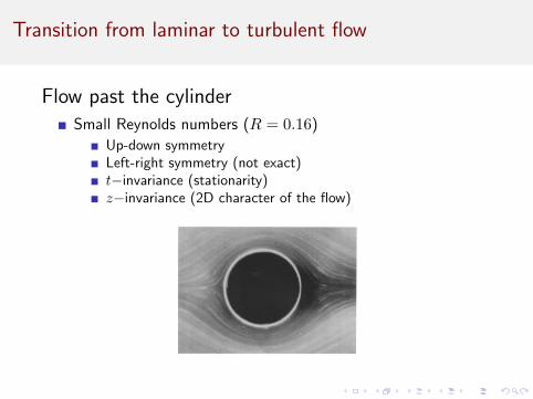
Transition from laminar to turbulent flow

Flow past the cylinderSmall Reynolds numbers (R = 0.16)

Up-down symmetryLeft-right symmetry (not exact)t−invariance (stationarity)z−invariance (2D character of the flow)

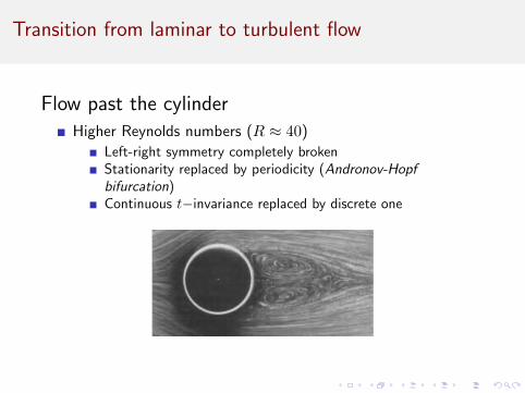
Transition from laminar to turbulent flow

Flow past the cylinderHigher Reynolds numbers (R ≈ 40)

Left-right symmetry completely brokenStationarity replaced by periodicity (Andronov-Hopfbifurcation)Continuous t−invariance replaced by discrete one

Transition from laminar to turbulent flow

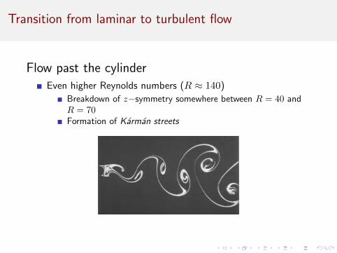
Flow past the cylinderEven higher Reynolds numbers (R ≈ 140)

Breakdown of z−symmetry somewhere between R = 40 andR = 70Formation of Karman streets

Transition from laminar to turbulent flow

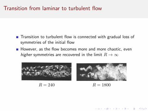
Transition to turbulent flow is connected with gradual loss ofsymmetries of the initial flow

However, as the flow becomes more and more chaotic, evenhigher symmetries are recovered in the limit R→∞

R = 240 R = 1800

Fully developed turbulence

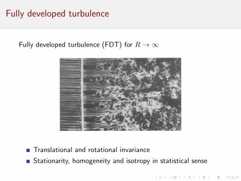
Fully developed turbulence (FDT) for R→∞

Translational and rotational invariance

Stationarity, homogeneity and isotropy in statistical sense

Kolmogorov theory

Phenomenological picture of FDT

Three scales

Dissipation scale rdDissipation of energy by viscosityMolecular scale

External scale rlScale of energy injectionCreation of large eddies

Inertial range rd � r � rl

Transfer of energy from large scales to the smaller onesGoverned by non-linearity of the NS equation

Kolmogorov theory

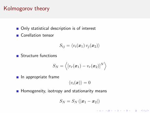
Only statistical description is of interest

Corellation tensor

Sij = 〈vi(x1) vj(x2)〉

Structure functions

SN =⟨

[vr(x1)− vr(x2)]N⟩

In appropriate frame〈vi(x)〉 = 0

Homogeneity, isotropy and stationarity means

SN = SN (|x1 − x2|)

Kolmogorov theory

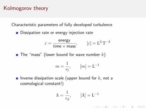
Characteristic parameters of fully developed turbulence

Dissipation rate or energy injection rate

ε =energy

time×mass, [ε] = L2 T−3

The “mass” (lower bound for wave number k)

m =1

rl, [m] = L−1

Inverse dissipation scale (upper bound for k, not acosmological constant!)

Λ =1

rd, [Λ] = L−1

Kolmogorov theory

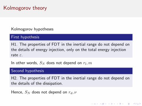
Kolmogorov hypotheses

First hypothesis

H1. The properties of FDT in the inertial range do not depend onthe details of energy injection, only on the total energy injectionrate ε.

In other words, SN does not depend on rl,m

Second hypothesis

H2. The properties of FDT in the inertial range do not depend onthe details of the dissipation.

Hence, SN does not depend on rd, ν

Kolmogorov theory

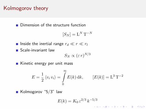
Dimension of the structure function

[SN ] = LN T−N

Inside the inertial range rd � r � rl

Scale-invariant lawSN ∝ (ε r)N/3

Kinetic energy per unit mass

E =1

2〈vi vi〉 =

∞∫0

E(k) dk, [E(k)] = L3 T−2

Kolmogorov “5/3” law

E(k) = K0 ε2/3 k−5/3

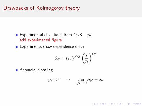
Drawbacks of Kolmogorov theory

Experimental deviations from “5/3” lawadd experimental figure

Experiments show dependence on rl

SN = (ε r)N/3(r

rl

)qNAnomalous scaling

qN < 0 → limr/rl→0

SN =∞

Path integrals: a brief review

Quantum mechanics in 1D

Propagator is the amplitude of probablity of

|q0〉 at time 0 −→ |q1〉 at time t

Definition

K(q1, t; q0, 0) =⟨q1 | e−i t H | q0

⟩Path integral expression

K(q1, t; q0, 0) =

∫Dq(t) ei S[q]

where S[q] is classical action

S[q] =

∫ [1

2m q2 − V (q)

]dt

Quantum field theory

Action for free scalar field

S0[φ] =

∫ [1

2(∂µφ) (∂µφ)− 1

2m2 φ2

]d4x

Green’s correlation functions

G(n)(x1, . . . xn) =⟨

0 | Tφ(x1) · · · φ(xn) | 0⟩

Path integral expression

G(n)(x1, . . . xn) =1

Z

∫φ(x1) . . . φ(xn) eiS[φ]Dφ

Quantum field theory

Generating functional for Green functions

G0[J ] =

∫eiS0[φ]+iJφDφ∫eiS0[φ]Dφ , Jφ ≡

∫φ(x) J(x) d4x

Generating functional

G0[J ] = eiS0[φc]+iJφc = e−12J ∆F J

where φc is classical solution of (� +m2)φc = J :

φc(x) = i

∫∆F (x, x′) J(x′) d4x′

Quantum field theory

Green functions can be derived from G0

G(n)(x1, . . . xn) =1

inδnG0[J ]

δJ(x1) . . . δJ(xn)

∣∣∣∣J=0

Taylor expansion

G0[J ] = e−12J∆F J = 1− 1

2J ∆F J +

1

8(J ∆F J)2 + . . .

One-point Green function

G(1)(x) =⟨

0 | φ(x) | 0⟩

=δG0

δJ(x)

∣∣∣∣J=0

= 0

Quantum field theory

Two-point Green function

G(2)(x1, x2) =⟨

0 | φ(x1) φ(x2) | 0⟩

= ∆F (x1, x2)

or diagramatically

G(2)(x1, x2) = x1 x2

Quantum field theory

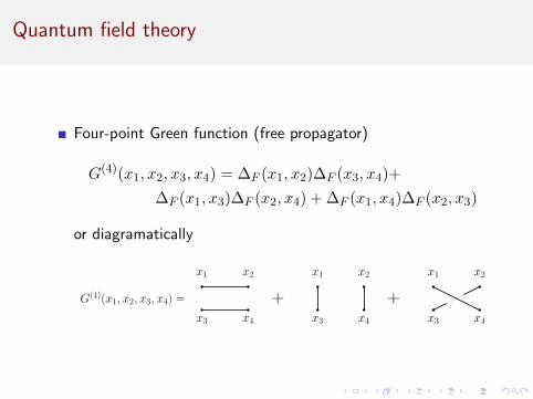
Four-point Green function (free propagator)

G(4)(x1, x2, x3, x4) = ∆F (x1, x2)∆F (x3, x4)+

∆F (x1, x3)∆F (x2, x4) + ∆F (x1, x4)∆F (x2, x3)

or diagramatically

G(4)(x1, x2, x3, x4) =

x1 x2

x3 x4

x1 x2

x3 x4

x1 x2

x3 x4

+ +

Quantum field theory

Self-interacting scalar field

S[φ] =

∫ [1

2(∂µφ)(∂µφ)− 1

2m2 φ2 − λ

4!φ4

]2-point Green’s function (to linear order in λ)

G(2) = ∆F (x1, x2)− i λ2

∫∆F (x1, x) ∆F (x, x) ∆F (x, x2) dx

Diagramatically

G(2)(x1, x2) =x1 x2 x1 x x2

+

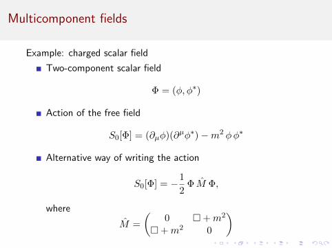
Multicomponent fields

Example: charged scalar field

Two-component scalar field

Φ = (φ, φ∗)

Action of the free field

S0[Φ] = (∂µφ)(∂µφ∗)−m2 φφ∗

Alternative way of writing the action

S0[Φ] = −1

2Φ M Φ,

where

M =

(0 � +m2

� +m2 0

)

Multicomponent fields

Generating functional

G0[J ] =1

Z

∫DΦ e−

i2

ΦMΦ+iJΦ

Again we introduce classical field Φc and find

G0[J ] = e−12

ΦcMΦc+iJΦc

where classical equations of motion are

MαβΦβ = Jα

{(� +m2)φ = Jφ(� +m2)φ∗ = Jφ∗

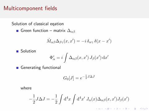
Multicomponent fields

Solution of classical eqation

Green function – matrix ∆αβ

Mαβ∆βγ(x, x′) = −i δαγ δ(x− x′)

Solution

Φcα = i

∫∆αβ(x, x′) Jβ(x′) dx′

Generating functional

G0[J ] = e−12J∆J

where

−1

2J∆J = −1

2

∫d4x

∫d4x′ Jα(x)∆αβ(x, x′)Jβ(x′)

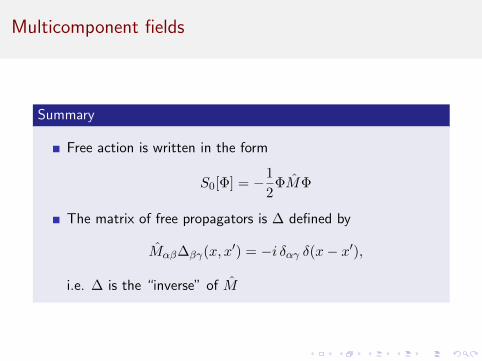
Multicomponent fields

Summary

Free action is written in the form

S0[Φ] = −1

2ΦMΦ

The matrix of free propagators is ∆ defined by

Mαβ∆βγ(x, x′) = −i δαγ δ(x− x′),

i.e. ∆ is the “inverse” of M

QFT formulation

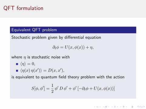
Equivalent QFT problem

Stochastic problem given by differential equation

∂tφ = U(x, φ(x)) + η,

where η is stochastic noise with

〈η〉 = 0,

〈η(x) η(x′)〉 = D(x, x′),

is equivalent to quantum field theory problem with the action

S[φ, φ′] =1

2φ′Dφ′ + φ′ [−∂tφ+ U(x, φ(x))]

QFT formulation

Stochastic incompressible Navier-Stokes equation

∂tvi + vj∂jvi = −∂iP + ν∆vi + fi

f is stochastic stirring force

Incompressibility implies

P = −∂i∂j∆

(vivj)

so that the transversal part of Navier-Stokes equation is

∂tvi + vj∂jvi = ν∆vi + fi

QFT formulation

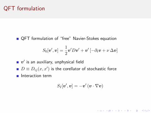
QFT formulation of “free” Navier-Stokes equation

S0[v′,v] =1

2v′Dv′ + v′ [−∂tv + ν∆v]

v′ is an auxiliary, unphysical field

D ≡ Dij(x, x′) is the corellator of stochastic force

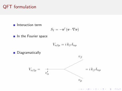
Interaction term

SI [v′,v] = −v′ (v · ∇v)

QFT formulation

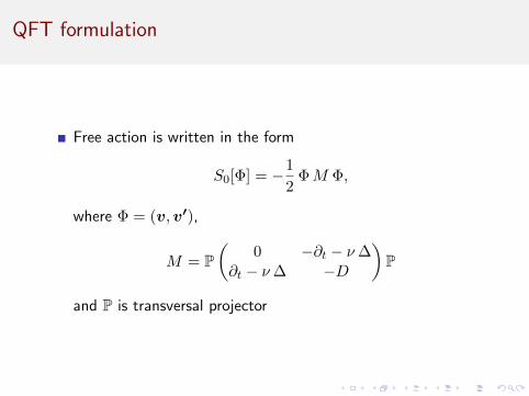
Free action is written in the form

S0[Φ] = −1

2ΦM Φ,

where Φ = (v,v′),

M = P(

0 −∂t − ν∆∂t − ν∆ −D

)P

and P is transversal projector

QFT formulation

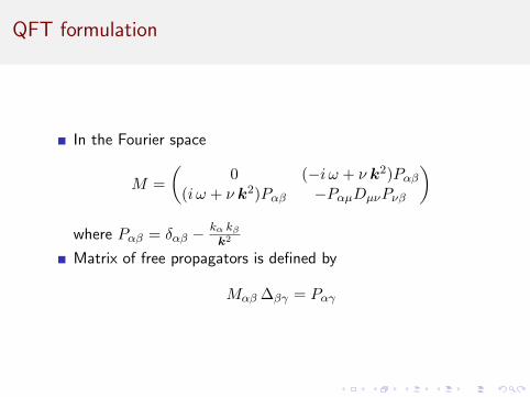
In the Fourier space

M =

(0 (−i ω + ν k2)Pαβ

(i ω + ν k2)Pαβ −PαµDµνPνβ

)where Pαβ = δαβ − kα kβ

k2

Matrix of free propagators is defined by

Mαβ ∆βγ = Pαγ

QFT formulation

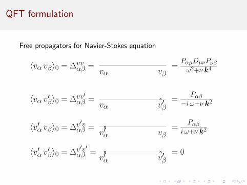
Free propagators for Navier-Stokes equation

=PαµDµνPνβω2+ν k4〈vα vβ〉0 = ∆vv

αβ =vα vβ

=Pαβ

−i ω+ν k2〈vα v′β〉0 = ∆vv′αβ =

vα v′β

=Pαβ

i ω+ν k2〈v′α vβ〉0 = ∆v′vαβ =

v′α vβ

= 0〈v′α v′β〉0 = ∆v′v′αβ =

v′α v′β

QFT formulation

Interaction termSI = −v′ (v · ∇v)

In the Fourier space

Vαβµ = i kβ δαµ

Diagramatically

v′α

vβ

vµ

Vαβµ = = i kβ δαµ

QFT formulation

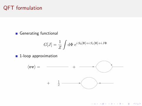
Generating functional

G[J ] =1

Z

∫dΦ ei S0[Φ]+i SI [Φ]+i JΦ

1-loop approximation

〈vv〉 = +

+ 12

QFT formulation

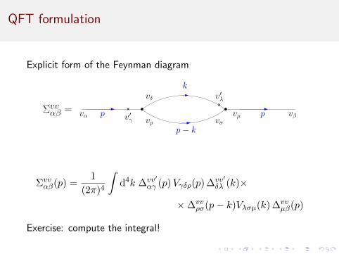
Explicit form of the Feynman diagram

vα v′γp

k

p− kp

vδ

vρ

v′λ

vσvβvµ

Σvvαβ =

Σvvαβ(p) =

1

(2π)4

∫d4k ∆vv′

αγ (p)Vγδρ(p) ∆vv′δλ (k)×

×∆vvρσ(p− k)Vλσµ(k) ∆vv

µβ(p)

Exercise: compute the integral!

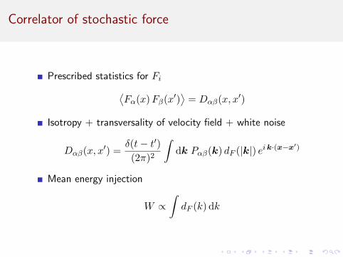
Correlator of stochastic force

Prescribed statistics for Fi⟨Fα(x)Fβ(x′)

⟩= Dαβ(x, x′)

Isotropy + transversality of velocity field + white noise

Dαβ(x, x′) =δ(t− t′)

(2π)2

∫dk Pαβ(k) dF (|k|) eik·(x−x′)

Mean energy injection

W ∝∫dF (k) dk

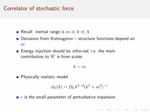
Correlator of stochastic force

Recall: inertial range is m� k � Λ

Deviation from Kolmogorov – structure functions depend onm

Energy injection should be infra-red, i.e. the maincontribution to W is from scales

k ∼ m

Physically realistic model

dF (k) = D0 k4−d(k2 +m2)−ε

ε is the small parameter of perturbative expansion

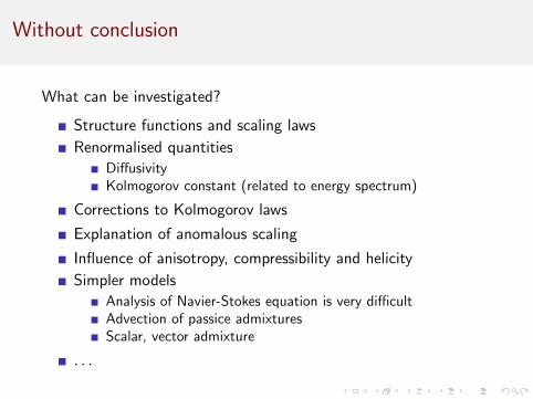
Without conclusion

What can be investigated?

Structure functions and scaling laws

Renormalised quantities

DiffusivityKolmogorov constant (related to energy spectrum)

Corrections to Kolmogorov laws

Explanation of anomalous scaling

Influence of anisotropy, compressibility and helicity

Simpler models

Analysis of Navier-Stokes equation is very difficultAdvection of passice admixturesScalar, vector admixture

. . .