quantitative macroeconomics: an introduction (2).pdf · quantitative macroeconomics: an...

Quantitative Macroeconomics: An Introduction

Dirk Krueger1

Department of EconomicsUniversity of Pennsylvania

April 2007

1The Author thanks Jesus Fernandez Villaverde for sharing much of his materialon the same issue. This book is dedicated to my son Nicolo. c by Dirk Krueger.

Contents

I Motivation and Data 1

1 Introduction 31.1 The Questions . . . . . . . . . . . . . . . . . . . . . . . . . . . . 31.2 The Approach and the Structure of the Book . . . . . . . . . . . 3

2 Basic Business Cycle Facts 52.1 Decomposition of Growth Trend and Business Cycles . . . . . . . 52.2 Basic Facts . . . . . . . . . . . . . . . . . . . . . . . . . . . . . . 15

II The Real Business Cycle (RBC) Model and Its Ex-tensions 17

3 Set-Up of the Basic Model 213.1 Households . . . . . . . . . . . . . . . . . . . . . . . . . . . . . . 213.2 Firms . . . . . . . . . . . . . . . . . . . . . . . . . . . . . . . . . 243.3 Aggregate Resource Constraint . . . . . . . . . . . . . . . . . . . 273.4 Competitive Equilibrium . . . . . . . . . . . . . . . . . . . . . . . 273.5 Characterization of Equilibrium . . . . . . . . . . . . . . . . . . . 30

4 Social Planner Problem and Competitive Equilibrium 334.1 The Social Planner Problem . . . . . . . . . . . . . . . . . . . . . 334.2 Characterization of Solution . . . . . . . . . . . . . . . . . . . . . 344.3 The Welfare Theorems . . . . . . . . . . . . . . . . . . . . . . . . 354.4 Appendix: More Rigorous Math . . . . . . . . . . . . . . . . . . 36

5 Steady State Analysis 395.1 Characterization of the Steady State . . . . . . . . . . . . . . . . 395.2 Golden Rule and Modi�ed Golden Rule . . . . . . . . . . . . . . 40

6 Dynamic Analysis 436.1 An Example with Analytical Solution . . . . . . . . . . . . . . . 446.2 Linearization of the Euler Equation . . . . . . . . . . . . . . . . . 47

6.2.1 Preliminaries . . . . . . . . . . . . . . . . . . . . . . . . . 476.2.2 Doing the Linearization . . . . . . . . . . . . . . . . . . . 48

iii

iv CONTENTS

6.3 Analysis of the Results . . . . . . . . . . . . . . . . . . . . . . . . 546.3.1 Plotting the Policy Function . . . . . . . . . . . . . . . . 546.3.2 Impulse Response Functions . . . . . . . . . . . . . . . . . 546.3.3 Simulations . . . . . . . . . . . . . . . . . . . . . . . . . . 54

6.4 Summary . . . . . . . . . . . . . . . . . . . . . . . . . . . . . . . 56

7 A Note on Economic Growth 577.1 Preliminary Assumptions and De�nitions . . . . . . . . . . . . . 577.2 Reformulation of Problem in E¢ ciency Units . . . . . . . . . . . 587.3 Analysis . . . . . . . . . . . . . . . . . . . . . . . . . . . . . . . . 607.4 The Balanced Growth Path . . . . . . . . . . . . . . . . . . . . . 60

8 Calibration 638.1 Long Run Growth Rates . . . . . . . . . . . . . . . . . . . . . . . 638.2 Capital and Labor Share . . . . . . . . . . . . . . . . . . . . . . . 648.3 The Depreciation Rate . . . . . . . . . . . . . . . . . . . . . . . . 648.4 The Technology Constant A . . . . . . . . . . . . . . . . . . . . . 658.5 Preference Parameters . . . . . . . . . . . . . . . . . . . . . . . . 658.6 Summary . . . . . . . . . . . . . . . . . . . . . . . . . . . . . . . 66

9 Adding Labor Supply 679.1 The Modi�ed Social Planner Problem . . . . . . . . . . . . . . . 679.2 Labor Lotteries . . . . . . . . . . . . . . . . . . . . . . . . . . . . 689.3 Analyzing the Model with Labor . . . . . . . . . . . . . . . . . . 699.4 A Note on Calibration . . . . . . . . . . . . . . . . . . . . . . . . 729.5 Intertemporal Substitution of Labor Supply: A Simple Example 739.6 A Remark on Decentralization . . . . . . . . . . . . . . . . . . . 74

10 Stochastic Technology Shocks: The Full RBC Model 7710.1 The Basic Idea . . . . . . . . . . . . . . . . . . . . . . . . . . . . 7710.2 Specifying a Process for Technology Shocks . . . . . . . . . . . . 7810.3 Analysis . . . . . . . . . . . . . . . . . . . . . . . . . . . . . . . . 8010.4 What are these Technology Shocks and How to Measure Them? . 82

III Evaluating the Model 85

11 Technology Shocks and Business Cycles 8911.1 Impulse Response Functions . . . . . . . . . . . . . . . . . . . . . 8911.2 Comparing Business Cycle Statistics of Model and Data . . . . . 9211.3 Counterfactual Experiments . . . . . . . . . . . . . . . . . . . . . 94

IV Welfare and Policy Questions 95

12 The Cost of Business Cycles 99

List of Figures

2.1 Natural Logarithm of real GDP for the US, in constant 2000 prices. 62.2 Deviations of Real GDP from Linear Trend, 1947-2004 . . . . . . 92.3 Growth Rates of Real GDP for the US, 1947-2004 . . . . . . . . 102.4 Trend Component of HP-Filtered Real GDP for the US, 1947-2004 132.5 Cyclical Component of HP-Filtered Real GDP for the US, 1947-

2004 . . . . . . . . . . . . . . . . . . . . . . . . . . . . . . . . . . 14

6.1 Dynamics of the Neoclassical Growth Model . . . . . . . . . . . . 466.2 Impulse Response Function for Capital . . . . . . . . . . . . . . . 55

11.1 Impulse Response Function for the Hansen Model, Shock to Capital 9011.2 Implulse Response for the Hansen Model, Technology Shock . . . 9111.3 Simulated Data from the Hansen Model . . . . . . . . . . . . . . 93

v

vi LIST OF FIGURES

List of Tables

2.1 Cyclical Behavior of Real GDP, US, 1947-2004 . . . . . . . . . . 15

8.1 Parameter Values . . . . . . . . . . . . . . . . . . . . . . . . . . 66

9.1 Labor and Consumption Allocations . . . . . . . . . . . . . . . . 74

11.1 Business Cycles: Data and Model . . . . . . . . . . . . . . . . . 93

vii

viii LIST OF TABLES

Preface

In these notes I will describe how to use standard neoclassical theory to explainbusiness cycle �uctuations.

ix

x LIST OF TABLES

Part I

Motivation and Data

1

Chapter 1

Introduction

1.1 The Questions

Business cycles are both important and, despite a large amount of economicresearch, still incompletely understood. While we made progress since the fol-lowing quote

The modern world regards business cycles much as the ancientEgyptians regarded the over�owing of the Nile. The phenomenonrecurs at intervals, it is of great importance to everyone, and naturalcauses of it are not in sight. (John Bates Clark, 1898)

there is still a lot that remains to be learned. In this class we will ask, andtry to at least try to partially answer the following questions

� What are them empirical characteristics of business cycles?

� What brings business cycles about?

� What propagates them?

� Who is most a¤ected and how large would be the welfare gains of elimi-nating them?

� What can economic policy, both �scal and monetary policy do in order tosoften or eliminate business cycles?

� Should the government try to do so?

1.2 The Approach and the Structure of the Book

Our methodological approach will be to use economic theory and empiricaldata to answer these questions. We will proceed in four basic steps with our

3

4 CHAPTER 1. INTRODUCTION

analysis. First we will document the stylized facts that characterize businesscycles in modern societies. Using real data, mostly for the US where the datasituation is most favorable we will �rst discuss how to separate business cycle�uctuations and economic growth from the data on economic activity, especiallyreal gross domestic product. The method for doing so is called �ltering. Ourstylized facts will be quantitative in nature, that is, we will not be content withsaying that the growth rate of real GDP goes up and down, but we want toquantify these �uctuations, we want to document how long a business cyclelasts, whether recessions and expansions last equally long, and how large andsmall growth rates of real GDP or deviations from the long run growth trend are.In a second step we will then construct a theoretical business cycle model thatwe will use to explain business cycles. We will build up this model up in severalsteps, starting as a benchmark with the neoclassical growth model. At each stepwe will evaluate how well the model does in explaining business cycles from aquantitative point. In the process we will also have to discuss how our modelis best parameterized (a process we will either call calibration or estimation,depending on the exact procedure) and how it is solved (it will turn out that wewill not always be able to deal with our model analytically, but sometimes willhave to resort to numerical techniques to solve the model). Into the basic growthmodel we will �rst introduce technology shocks and endogenous labor supply,which leads us to the canonical Real Business Cycle Model. Further extensionswill include capital adjustment costs, two sector models and sticky prices andmonopolistic competition. Once the last two elements are incorporated intothe model we have arrived at the New Keynesian business cycle model. Ina third step we will then evaluate the ability of the di¤erent versions of themodel to generate business cycles of realistic magnitude. Once the model(s)do a satisfactory job in explaining the data, we can go on and ask normativequestions. The �nal fourth step of our analysis will �rst quantify how largethe welfare costs of business cycles are and then analyze, within our models,how e¤ective monetary and �scal policy is to tame cyclical �uctuations of theeconomy.

Chapter 2

Basic Business Cycle Facts

In this chapter we want to accomplish two things. First we will discuss how todistill business cycle facts from the data. The main object of macroeconomistsis aggregate economic activity, that is, total production in an economy. This isusually measured by real GDP or, if one is more interested in living standardsof households, by real GDP per capita or worker. But plotting the time seriesof real GDP we see that not only does it �uctuate over time, but it also has asecular growth trend, that it, is goes up on average. For the study of businesscycle we have to purge the data from this long run trend, that is, take it out ofthe data. The procedure for doing so is called �ltering, and we will discuss howto best �lter the data in order to divide the data into a long run growth trendand business cycle �uctuations.Second, after having de-trended the data, we want to take the business cycle

component of the data and document the main stylized facts of business cycles,that is, study what are the main characteristics of business cycles. We wantto document the length of a typical business cycle, whether the business cycleis symmetric, the size of deviations from the long run growth trend, and thepersistence of deviations from the long-run growth trend.

2.1 Decomposition of Growth Trend and Busi-ness Cycles

In Figure 2.1 we plot the natural logarithm of real GDP for the US from 1947to 2004. The reason we start with US data, besides it representing the biggesteconomy in the world, is that the data situation for this country is quite favor-able. There are no obvious trend breaks, due to, say, major wars, change inthe geographic structure of the country (such as the German uni�cation), andreal data are available with consistent de�ation for price changes over the entiresample period. In exercises you will have the opportunity to study your countryof choice, but you should be warned already that for Germany consistent datafor real GDP are available only for much shorter time periods (not least because

5

6 CHAPTER 2. BASIC BUSINESS CYCLE FACTS

of the German uni�cation).

1950 1960 1970 1980 1990 2000

7.4

7.6

7.8

8

8.2

8.4

8.6

8.8

9

9.2

9.4

Time

Nat

ural

Log

Rea

l GD

P, i

n $

Real GDP, in 2000 Prices, Quaterly Frequency

DataLinear Trend

Figure 2.1: Natural Logarithm of real GDP for the US, in constant 2000 prices.

A short discussion of the data themselves. The frequency of the data is quar-terly, that is, we have one observation fro real GDP in each quarter. However,the observation is for real GDP for the preceding twelve months, not just thelast three months. In that way seasonal in�uences on GDP are controlled for.The base year for the data is 2000, that is, all numbers are in 2000 US dollars.In terms of units, the data are in billion US dollars (Milliarden). For examplefor 2004 real GDP is about

exp(9:3) � $10:000 Billion = $10 Trillion

or about $36; 000 per capita. Finally, why would we plot the natural logarithmof the data, rather than the data themselves. Here is the reason: suppose aneconomic variable, say real GDP, denoted by Y; grows at a constant rate, say g,

2.1. DECOMPOSITION OF GROWTH TREND AND BUSINESS CYCLES7

over time. Then we haveYt = (1 + g)

tY0 (2.1)

where Y0 is real GDP at some starting date of the data, and Yt is real GDP inperiod t: Now let us take logs (and whenever I say logs, I mean natural logs, thatis, the logarithm with base e; where e � 2:781 is Euler�s constant) of equation(2:1): This yields

log(Yt) = log�(1 + g)tY0

�= log(Y0) + log

�(1 + g)t

�= log(Y0) + t � log [1 + g]

where we made use of some basic rules for logarithms.What is important about this is that if a variable, say real GDP, grows at

a constant rate g over time, then if we plot the logarithm of that variable it isexactly a straight line with intercept Y0 and slope

slope = log(1 + g) � g

where the approximation in the last equation is quite accurate as long as g isnot too large.1 Similarly, we need not start at time s = 0: Suppose our datastarts at an arbitrary date s (in the example s = 1947). Then if our data growsat a constant rate g; the �gure for log(Yt) is given by

log(Yt) = log(Ys) + (t� s) log(1 + g);

and if s = 1947; then

log(Yt) = log(Y1947) + (t� 1947) log(1 + g)

Thus, if real GDP grew at a constant rate, a plot of the natural logarithm ofreal GDP should be straight line, with slope equal to the constant growth rate.Figure 2.1 shows that this is not too bad of a �rst approximation.In this course, however, we are mostly interested in the deviations of actual

real GDP from its long run growth trend. First we want to mention that thedecision what part of the data is considered a growth phenomenon and whatis considered a business cycle phenomenon is somewhat arbitrary. To quoteCooley and Prescott (1995)

1The fact that log(1 + g) � g can be seen from the Taylor series expansion of log(1 + g)around g = 0: This yields

log(1 + g) = log(1) +g � 01

� 1

2(g � 0)2 + 1

6(g � 0)3 + : : :

= g � 1

2g2 +

1

6g3 + : : :

� g

because the terms where g is raised to a power are small relative to g; whenever g is nottoo big.


Every researcher who has studied growth and/or business cycle�uctuations has faced the problem of how to represent those featuresof economic data that are associated with long-term growth andthose that are associated with the business cycle - the deviationfrom the growth path. Kuznets, Mitchell and Burns and Mitchell[early papers on business cycles] all employed techniques (movingaverages, piecewise trends etc.) that de�ne the growth componentof the data in order to study the �uctuations of variables around thelong-run growth path de�ned by the growth component. Whateverchoice one makes about this is somewhat arbitrary. There is nosingle correct way to represent these components. They ares implydi¤erent features of the same observed data.

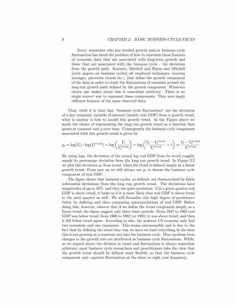
Thus, while it is clear that �business cycle �uctuations� are the deviationof a key economic variable of interest (mostly real GDP) from a growth trend,what is unclear is how to model this growth trend. In the Figure above wemade the choice of representing the long run growth trend as a function thatgrows at constant rate g over time. Consequently the business cycle componentassociated with this growth trend is given by

yt = log(Yt)�log(Y trendt ) = log

�Yt

Y trendt

�= log

�Yt � Y trendt

Y trendt

+ 1

�� Yt � Y trendt

Y trendt

By using logs, the deviation of the actual log real GDP from its trend roughlyequals its percentage deviation from the long run growth trend. In Figure 2.2we plot this deviation yt from trend, when the trend is de�ned simply as a lineargrowth trend. From now on we will always use yt to denote the business cyclecomponent of real GDP.The �gure shows that business cycles, so de�ned, are characterized by fairly

substantial deviations from the long run growth trend. The deviations havemagnitudes of up to 10%; and they are quite persistent: if in a given quarter realGDP is above trend, it looks as if it is more likely that real GDP is above trendin the next quarter as well. We will formalize this high degree of persistencebelow by de�ning and then computing autocorrelations of real GDP. Beforedoing this, however, observe that if we de�ne the trend component simply as alinear trend, the �gure suggest only three basic periods. From 1947 to 1965 realGDP was below trend, from 1966 to 1982 (or 1991) it was above trend, and thenit fell below trend again. According to this, the postwar US economy only hadtwo recessions and one expansion. This seems unreasonable and is due to thefact that by de�ning the trend they way we have we load everything in the datathis is not growing at a constant rate into the business cycle. More medium termchanges in the growth rate are attributed as business cycle �uctuations. While,as we argued above the division in trend and �uctuations is always somewhatarbitrary, most business cycle researchers and practitioners take the view thatthe growth trend should be de�ned more �exibly, so that the business cyclecomponent only captures �uctuations at the three to eight year frequency.


1950 1960 1970 1980 1990 2000

10

8

6

4

2

0

2

4

6

8

Time

Perc

enta

ge D

evia

tion

from

Tre

nd

Real GDP, Deviation from Trend, Quaterly Frequency

Zero LineDeviation from Trend

Figure 2.2: Deviations of Real GDP from Linear Trend, 1947-2004

So in practice most business cycle researchers measure business cycle �uctu-ations using one of three statistics: a) growth rates of real GDP, b) the cyclicalcomponent of Hodrick-Prescott �ltered data, c) the data component of the ap-propriate frequency of a band pass �lter. We will discuss the �rst two of thesemethods, and only brie�y mention the third, because its understanding requiresa discussion of spectral methods which you may know if you studied physics ora particular area of �nance, but which I do not want to teach in this class.

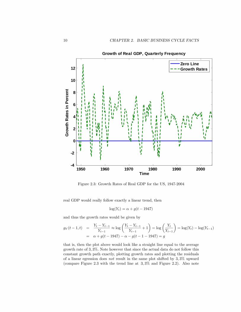
Figure 2.3 plots growth rates of real GDP for the US. Remember that eventhough the data frequency is quarterly, these are growth rates for yearly realGDP. The average growth rate over the sample period is 3; 3%: As a side remark,about one third of this growth is due to population and thus labor force growth,and two thirds are due to higher real GDP per capita. Note that if the log of


1950 1960 1970 1980 1990 20004

2

0

2

4

6

8

10

12

Time

Gro

wth

Rat

es in

Per

cent

Growth of Real GDP, Quarterly Frequency

Zero LineGrowth Rates

Figure 2.3: Growth Rates of Real GDP for the US, 1947-2004

real GDP would really follow exactly a linear trend, then

log(Yt) = �+ g(t� 1947)

and thus the growth rates would be given by

gY (t� 1; t) =Yt � Yt�1Yt�1

� log�Yt � Yt�1Yt�1

+ 1

�= log

�YtYt�1

�= log(Yt)� log(Yt�1)

= �+ g(t� 1947)� �� g(t� 1� 1947) = g

that is, then the plot above would look like a straight line equal to the averagegrowth rate of 3; 3%: Note however that since the actual data do not follow thisconstant growth path exactly, plotting growth rates and plotting the residualsof a linear egression does not result in the same plot shifted by 3; 3% upward(compare Figure 2.3 with the trend line at 3; 3% and Figure 2.2). Also note


that, when dealing with yt = log(Yt); computing the growth rate

gY (t� 1; t) = log(Yt)� log(Yt�1) = yt � yt�1

amounts to plotting the data in deviations from its value in the previous quarter.Thus e¤ectively all variations of the data longer than one quarter are �ltered outby this procedure, leaving only the very highest frequency �uctuations behind.This is why the plot looks very �jumpy�, and observations in successive quartersnot very correlated. We will document this fact more precisely below.While the popular discussion mostly uses growth rates to talk about the

state of the business cycle, academic economists tend to separate growth andcycle components of the data by applying a �lter to the data. In fact, specifyingthe deterministic constant growth trend above and interpreting the deviationsas cycle was nothing else than applying one such, fairly heuristic �lter to thedata. One �lter that has enjoyed widespread popularity is the so-called Hodrick-Prescott �lter, or HP-�lter, for short. The goal of the �lter is as before : specifya growth trend such that the deviations from that trend can be interpreted asbusiness cycle �uctuations. Let us describe this �lter in more detail and tryto interpret what it does. As always we want to decompose the raw data,log(Yt) into a growth trend ytrendt = log(Y trendt ) and a cyclical componentyt = log(Y

cyclet ) such that

log(Yt) = log(Y trendt ) + log(Y cyclet )

yt = log(Yt)� ytrendt

Of course the key question is how to pick yt and ytrendt from the data? The HP-�lter proposes to make this decomposition by solving the following minimizationproblem

minfyt;ytrendt g

TXt=1

(yt)2+ �

TXt=1

�(ytrendt+1 � ytrendt )� (ytrendt � ytrendt�1 )

�2(2.2)

subject to

yt + ytrendt = log(Yt) (2.3)

where T is the last period of the data. Note that we are given the dataflog(Yt)gTt=0, so the right hand side of 2.3 is a known and given number, foreach time period. Implicit in this minimization problem is the following trade-o¤ in choosing the trend. We may want the trend component to be a smoothfunction, but we also may want to make the trend component track the actualdata to some degree, in order to capture also some �uctuations in the data thatare of lower frequency than business cycles. These two considerations are tradedo¤ by the parameter �: If � is big, we want to make the terms�

(ytrendt+1 � ytrendt )� (ytrendt � ytrendt�1 )�2


small. But the term

(ytrendt+1 � ytrendt )� (ytrendt � ytrendt�1 )

=�log(Y trendt+1 )� log(Y trendt )

��log(Y trendt )� log(Y trendt�1 )

�= gY trend(t; t+ 1)� gY trend(t� 1; t)

is nothing else but the change in the growth rate of the trend component. Thusa high � makes it optimal to have a trend component with fairly constant slope.In the extreme as � ! 1; the weight on the second term is so big that it isoptimal to set this term to 0 for all time periods, that is,

gY trend(t; t+ 1)� gY trend(t� 1; t) = 0

gY trend(t; t+ 1) = gY trend(t� 1; t) = g

and thus

ytrendt � ytrendt�1 = g

ytrendt = ytrendt�1 + g

for all time periods t: But this is nothing else but our constant growth lineartrend that we started with. This is, the HP-�lter has the linear trend as aspecial case.Now consider the other extreme, in which we value a lot the ability of the

trend to follow the real data. Suppose we set � = 0; then the objective functionto minimize becomes

minfyt;ytrendt g

TXt=1

(yt)2 subject to yt + ytrendt = log(Yt)

or substituting in for yt

minfytrendt g

TXt=1

�log(Yt)� ytrendt

�2and the solution evidently is

ytrendt = log(Yt)

that is, the trend is equal to the actual data series and the deviations fromthe trend, our business cycle �uctuations, are identically equal to zero. Theseextremes show that we want to pick a � bigger than zero (otherwise there areno business cycle �uctuations and all of the data are due to the long run trend)and smaller than 1 (so that the trend picks up some medium run variation inaddition to long run growth and does not leave everything but the longest runmovements to the �uctuations part).Thus which � to choose must be guided by our objective of �ltering out

business cycle �uctuations, that is, �uctuations in the data with frequency of


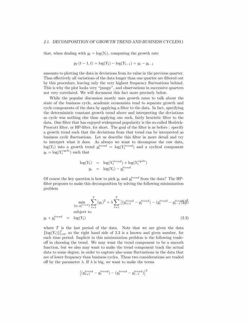
between three to �ve years. Which choice of � accomplishes this depends cru-cially on the frequency of the data; for quarterly data a value of � = 1600 iscommonly used, which loads into the trend component �uctuations that occurat frequencies of roughly eight years or longer. Note that for any � 2 (0;1) itis not completely straightforward to solve the minimization problem associatedwith the HP-�lter. But luckily there exists pre-programed computer code injust about any software package to do this.Figure 2.4 shows the trend component of the data, derived from the HP-

�lter with a smoothing parameter � = 1600: That is, the �gure plots ytrendt

against time. We observe that, in contrast to a simply constant growth trendthe HP-trend captures some of the medium frequency variation of the data,which was the goal of applying the HP-�lter in the �rst place. But the HPtrend component is still much smoother than the data themselves.

1950 1960 1970 1980 1990 2000

7.4

7.6

7.8

8

8.2

8.4

8.6

8.8

9

9.2

9.4

Time

Nat

ural

Log

Rea

l GD

P, i

n $

Real GDP in 2000 Prices, Quaterly Frequency

DataHodrickPrescott Trend

Figure 2.4: Trend Component of HP-Filtered Real GDP for the US, 1947-2004

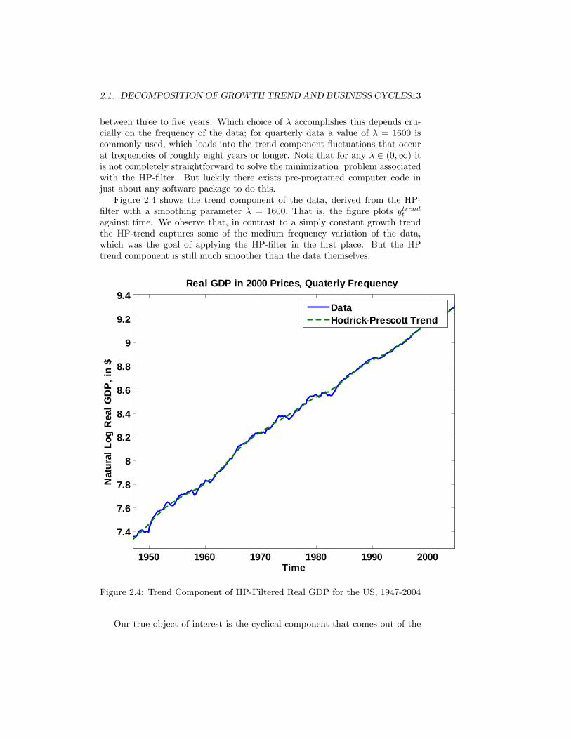
Our true object of interest is the cyclical component that comes out of the


HP �ltering Figure 2.5 displays the business cycle component of the HP-�ltereddata, yt: As in Figures 2.3 and 2.2 this �gure shows that the cyclical variationin real GDP can be sizeable, up to 4�6% in both directions from trend. Clearlyvisible are the mid-seventies and early eighties recessions, both partially due tothe two oil price shocks, the recession of the early 90�s that cost George W.Bush�s dad his job and the fairly mild (by historical standard) recent recessionin 2001.

1950 1960 1970 1980 1990 2000

6

4

2

0

2

4

Time

Perc

enta

ge D

evia

tions

Fro

m T

rend

Deviations of Real per Capita GDP, Quarterly Frequency

Zero LineHodrickPrescott Cycle

Figure 2.5: Cyclical Component of HP-Filtered Real GDP for the US, 1947-2004

But now we want to proceed with a more systematic collection of businesscycle facts. We �rst focus on our main variable of interest, real GDP. In laterchapters, once we enrich our benchmark model with labor supply and otherrealistic features, we will augment these facts with facts about other variablesof interest.

2.2. BASIC FACTS 15

Variable Mean St. Dv. A(1) A(2) A(3) A(4) A(5) min max %(>0) %(>0,033)Growth Rate 3:3% 2; 6% 0; 83 0; 54 0; 21 �0; 09 �0; 20 �3; 1% 12; 6% 88; 6% 54; 0%HP Filter 0% 1:7% 0; 84 0; 60 0; 32 0; 08 �0; 10 �6; 2% 3; 8% 53; 9% N=A

Table 2.1: Cyclical Behavior of Real GDP, US, 1947-2004

2.2 Basic Facts

Now that we have discussed how to be measure business cycle facts, let usdocument the main regularities of business cycles. Sometimes the resulting factsare called stylized facts, that is, facts one gets from (sophisticatedly) eyeballingthe data. These facts will be the targets of comparison for our quantitativemodels to be constructed in the next part of this class. The goal of the modelsis to generate business cycles of realistic magnitude, and to explain what bringsthem about. In order to do so, we need empirical benchmark facts.

Table 2.1 summarizes the main stylized facts or quarterly real GDP for theUS between 1947 and 2004, both when using growth rates and when using thecyclical component of the HP-�ltered series. The mean and standard deviationof a time series fxtgTt=0 are de�ned as

mean(x) =1

T

TXt=0

xt

std(x) =

1

T

TXt=0

(xt �mean(x))2! 1

2

The autocorrelations are de�ned as follows

A(i) = corr(xt; xt�1) =1

T�iPt(xt �mean(x))(xt�i �mean(x))

std(x) � std(x)

and measure how persistent a time series is. For time series with high �rst orderautocorrelation tomorrow�s value is likely to be of similar magnitude as today�svalue. Finally the table gives the maximum and minimum of the time series andthe fraction of observations above zero, and, for the growth rate, the fraction ofobservations bigger than its mean, 3; 3%:We make the following observations. First, besides the fact that the mean

growth rate is 3; 3% whereas the cyclical component of the HP-�ltered serieshas a mean of 0; the main stylized facts derived from taking growth rates andHP-�ltering are about the same. They are:

1. Real GDP has a volatility of about 2% around trend, or more concretely,1; 7% when considering the HP-�ltered series.


2. The cyclical component of real GDP is highly persistent (that is, positivedeviations are followed with high likelihood with positive deviations). Theautocorrelation declines with the order and turns negative for the �fthorder (that is if real GDP is above trend this quarter, it is more likely tobe below than above trend in �ve quarters from now).

3. Positive deviations from trend are more likely than negative deviationsfrom trend. This suggests that recessions are short but sharp, whereasexpansions are long but gradual.

4. It is rare that the growth rate of real GDP actually becomes negative, atleast for the US between 1947 and 2004.

It is an instructive exercise (that you will do with Philip�s help) to carry outthe same empirical exercise described in these notes for an alternative countryof your choice. All you need is a su¢ ciently long time series for real GDP fora country (preferably seasonably adjusted), a little knowledge of MATLAB (orsome equivalent software package) and a pre-programed HP �lter subroutine(which for MATLAB I will give you). But now we want to start constructingour theoretical model that we will use to explain existence and magnitude ofthe business cycles documented above.

Part II

The Real Business Cycle(RBC) Model and Its

Extensions

17

19

In this part we describe the basic real business cycle model. We start withits simplest version, in which endogenous labor supply and technology shocksare absent. That version of the model is also known in the literature as theCass-Koopmanns neoclassical growth model. After setting up the model we willargue that the equilibrium of the model can be solved for by instead solving themaximization problem of a �ctitious benevolent social planner (and we will arguewhy this is much easier than solving for the equilibrium directly). We then willderive and study the basic optimality conditions from this model. We will startwith the explicit solution of the model by carrying out a steady state analysis,that is, we look for a special equilibrium in which the economic variables ofinterest (GDP, consumption, investment, the capital stock) are constant overtime. Since this steady state is also the starting point of our general discussion ofthe solution of the model, it is a natural starting point for the analysis. We thendiscuss how to solve for the entire dynamic behavior of the model, which requiressome mathematical and/or computational tricks. Then we quickly address howwe can, in a straightforward manner and without further complications, addtechnological progress and population growth to the model. This will concludethe basic theoretical discussion of the benchmark model.In order to make the model into an operational tool for business cycle analysis

we have to choose parameter values that specify the elements of the model(that is, the utility function of the household and the production technologyof the �rms). The rigorous method for doing so within the RBC traditionis called calibration (if time permits I will transgress into a discussion of themain di¤erences and relative advantages of calibration and formal econometricestimation). After parameterizing the model we are ready to use it. However,we will see that the benchmark model by construction does not deliver businesscycles nor �uctuations of employment over time. In order to rectify this wein turn introduce a labor supply decision and stochastic (random) productivityshocks into the model.

Chapter 3

Set-Up of the Basic Model

In the benchmark model there are two types of economic actors, private house-holds and �rms. Time is discrete and the economy lasts for T periods, whereT =1 (the economy lasts forever) is allowed. A typical time period is denotedby t: We now describe in turn private households and �rms in this economy.

3.1 Households

Households live for T periods. All households are completely identical, andfor simplicity we normalize the total number of households to 1: While thisspares us to divide all macroeconomic variables by the number of people toobtain per-capita values, you should think about the economy being populatedby many households that just happen to sum to 1: Where the assumption ofmany households is crucial is that it allows us to treat households as behavingcompetitively, that is, households believe that their actions do not a¤ect marketprices in the economy (because they have it in their head that there are so manyhouseholds in the economy that weight in the population is negligibly small).In the simple version of the model households simply decide in each period howmuch of their income to consume, and how much to save for tomorrow. Weassume that per period households can work a total of 1 unit of time, and sincethey don�t care about leisure they do work all the time.Let by ct denote the household�s consumption at time t:We assume that the

household has a utility function of the form

U(c0; c1; : : : ; cT ) = u(c0) + �u(c1) + �2u(c2) + : : :+ �

Tu(cT )

=TXt=0

�tu(ct)

where � 2 (0; 1) is the time discount factor. The fact that we assume � < 1indicates that our consumer is impatient; she derives less utility from the sameconsumption level if that consumption occurs later, rather than earlier in life.

21

22 CHAPTER 3. SET-UP OF THE BASIC MODEL

Sometime we will also measure the degree of the household�s impatience by thetime discount rate �: The time discount rate and the time discount factor arerelated via the equation

� =1

1 + �

We will make assumptions on the period utility function u later; for now weassume that is is at least twice di¤erentiable, strictly increasing and strictlyconcave (that is, u0(c) > 0 and u00(c) < 0 for all c). In applications we will oftenassume that the utility function is logarithmic, that is, u(c) = log(c); where logdenotes the natural logarithm. This assumption is made partially because itgives us simple solutions, partly because the solution we will get has some veryplausible properties.Now that we know what people like (consumption in all periods of their life),

we have to discuss what people can a¤ord to buy. Besides working one unit oftime per period and earning a wage wt; households are born with initial assetsa0 > 0: Their budget constraint in period t reads as

ct + at+1 = wt + (1 + rt)at

This equation tells us several things. First, we assume that the numeraire goodis the consumption good, and normalize its price to 1: Consequently assets arereal assets, that is, they pay out in terms of the consumption good, ratherthan in terms of money (the term money will be largely absent in this class).Similarly, wt is the real wage and rt is the real interest rate. The equation saysthat expenditures for consumption plus expenditures for purchases of assets thatpay out in period t+1; at+1; have to equal labor income wt �1 plus the principalplus interest of assets purchased yesterday and coming due today, (1 + rt)at:Another way of writing this is

ct + at+1 � at = wt + rtat

with the interpretation that labor income wt and capital income rtat are spenton consumption ct and savings at+1 � at (which is nothing else but the changein the asset position of the household between today and tomorrow). Finallynote that we allow the household to purchase only one asset, a real asset withmaturity of one period. In this simple model the introduction of other, morecomplicated assets would not change matters (i.e. the consumption allocation),but we leave the discussion of this to the many excellent asset pricing classesat Frankfurt). The household starts with assets a0 that are given exogenously(the household is simply born with it). But what about the end of life. Ifwe allow the household to die in debt, she would certainly decide to do so; infact, without any limit the household optimization problem has no solution asthe household would run up in�nitely high debt. We assume instead that thehousehold cannot die in debt, that is, we require aT+1 � 0: Since there is nopoint in leaving any assets unspent (the household is sel�sh and does not careabout potential descendants, plus she knows exactly when she is dying), weimmediately have aT+1 = 0: If the household lives forever, that is, T =1; then

3.1. HOUSEHOLDS 23

the terminal condition for assets is slightly more complicated; one has to ruleout that household debt does not grow to fast far in the future.1 We will skipthe details here; if interested, please refer to my Ph.D. lecture notes on the sameissue.This leaves us with the following household maximization problem: given

a time path of wages and interest rates fwt; rtgTt=0 and initial assets a0; thehousehold solves

maxfct;at+1gTt=0

TXt=0

�tu(ct)

subject to

ct + at+1 = wt + (1 + rt)at

ct � 0

aT+1 = 0

For future reference let us derive the necessary (and if T is �nite, these are alsothe su¢ cient) condition for an optimal consumption choice. First let us ignorethe non-negativity constraints on consumption and the terminal condition onassets (the latter one we will use below, and it is easy to make assumptions on theutility function that guarantees ct > 0 for all periods, such as limc!0 u

0(c) =1).Setting up the Lagrangian, with �t denoting the Lagrange multiplier on theperiod t budget constraint gives

L =

TXt=0

�tu(ct) +

TXt=0

�t (wt + (1 + rt)at � ct � at+1)

Taking �rst order conditions with respect to ct with respect to ct+1 and withrespect to at+1 and setting them to zero yields

�tu0(ct) = �t

�t+1u0(ct+1) = �t+1

�t = �t+1(1 + rt+1)

Combining these equations yields the standard intertemporal consumption Eulerequation

u0(ct) = �(1 + rt+1)u0(ct+1) (3.1)

This equation has the standard interpretation that if the household choosesconsumption optimally, she exactly equates the cost from saving one more unittoday (the loss of u0(ct) utils) to the bene�t (saving one more unit of con-sumption today gives 1 + rt+1 more units of consumption tomorrow, and thus(1 + rt+1) � �u0(ct+1) more utils).

1A condition to rule this out is sometimes called a no Ponzi condition, in honor of a Bostonbusiness man and criminal that e¤ectively tied to borrow without bounds. His so-called Ponzischeme eventually exploded.


We will often be interested in a situation where the economic variables ofinterest, here consumption and the interest rate, are constant over time, thatis, ct = ct+1 = c and rt+1 = r: Such a situation is often called a steady state.From the previous equation we see right away that a steady state requires

u0(c) = �(1 + r)u0(c)

or1 = �(1 + r)

That is, in a steady state the time discount rate � necessarily has to equalthe interest rate, � = r; because only at that interest rate will households �ndit optimal to set consumption constant over time (what happens if � > r or� < r?). Of course the reverse is also true: if rt = � for all time periods, itfollows that consumption is constant over time.Finally we can characterize the entire dynamics of consumption, savings

and asset holdings of the household, even though we may need assumptions,mathematical tricks or a computer to solve for them explicitly. Solving thebudget constraint for consumption yields

ct = wt + (1 + rt)at � at+1ct+1 = wt+1 + (1 + rt+1)at+1 � at+2

Inserting these into equation (3:1) yields

u0(wt + (1 + rt)at � at+1) = �(1 + rt+1)u0(wt+1 + (1 + rt+1)at+1 � at+2) (3.2)

Remember that the household takes wages and interest rates fwt; rtgTt=0 as givennumbers; thus the only choice variables in this equation are at; at+1; at+2:Math-ematically, this is a second order di¤erence equation (unfortunately a nonlinearone in general). But we have an initial condition (since a0 is exogenously given)and a terminal condition, aT+1 = 0; so in principle we can solve this secondorder di¤erence equation (in practice, as mentioned above, we either pick theutility function and thus u0 well), rely on some mathematical approximationsor switch on a computer and program an algorithm that solves this di¤erenceequation boundary problem. We will return to this problem below.

3.2 Firms

As with households we assume that all �rms are identical and normalize thenumber of �rms to 1: Again we still assume that �rms believe to be so smallthat their hiring decisions do not a¤ect the wages they have to pay their workersand the rental price they have to pay for their capital. The representative �rm ineach period produces the consumption good households like to eat. Let yt denotethe output of the �rm of this consumption good, and nt denote the number ofworkers being hired by the �rm, and kt the amount of physical capital (machines,

3.2. FIRMS 25

buildings) being used in production at period t: The production technology isdescribed by a standard neoclassical Cobb-Douglas production function

yt = Atk�t n

1��t

Here At is a technology parameter that determines, for a given input, how muchoutput is being produced. For now we assume that At = A > 0 is constant overtime. Below we will then introduce shocks to At to generate business cycles.The fact that these shocks are shocks to the production technology and thus�real�shocks (as opposed to, say, monetary shocks), gives the resulting businesscycle theory its name Real Business Cycle Theory. But for now the productiontechnology is given by

yt = Ak�t n1��t

The parameter � measures the importance of the capital input in production2 ;we will link it to the capital share of income below. In addition, when the �rmuses kt machines in period t; a fraction � of them wear down. This process iscalled depreciation. Also note that this production function exhibits constantreturns to scale: doubling both inputs results in doubled output.The �rm hires workers at a wage wt per unit of time; for simplicity we also

assume that the �rm rents the capital it uses in the production process fromthe households, rather than owning the capital stock itself. This turns out to bean inconsequential assumption and makes our life easier when stating the �rm�sproblem. Thus from now on we identify the asset the household saves with asthe physical capital stock of the economy. Let the rental price per unit of capitalbe denoted by �t: Note that because of depreciation, whenever a household rentsone machine to the �rm, she receives �t� � as e¤ective rental payment (since afraction � of the machine disappears in the production process and thus is notreturned back to the household). The rental rate of capital and the real interestrate then satisfy the relation

rt = �t � �:

The �rm takes wages and rental rates of capital as given and maximizes periodby period pro�ts (there is nothing dynamic about the �rm, as it rents all inputs

2Note that � is in fact the elasticity of output with respect to the capital input. Take logsof the production function to obtain

log(yt) = log(A) + � log(kt) + (1� �) log(nt)

and thusd log(yt)

d log(kt)= �:

Similarlyd log(yt)

d log(nt)= 1� �


period by period and sells output period by period):

maxnt;kt

(yt � wtnt � �tkt)

subject to


kt; nt � 0

Again ignoring the nonnegativity constraints on inputs (given the form of theproduction function, these are never binding -why?) the maximization problembecomes

maxnt;kt

�Ak�t n

1��t � wtnt � �tkt

�with �rst order conditions

wt = (1� �)A�ktnt

��t = �A

�ktnt

��1: (3.3)

That is, �rms set their inputs such that they equate the wage rate (which theytake as exogenously given) to the marginal product of labor. Likewise the rentalrate of capital is equated to the marginal product of capital. An easy calculationshows that the pro�ts of the �rm equal

�t = Ak�t n1��t � wtnt � �tkt

= Ak�t n1��t � (1� �)A

�ktnt

��nt � �A

�ktnt

��1kt

= 0:

In fact, knowing this beforehand in the household problem above I never in-cluded pro�ts of �rms in the budget constraint. Likewise I never discussed whoowns these �rms. Given that their pro�ts happen to equal zero, this is irrelevant.Note that the zero pro�t result does not hinge on the Cobb-Douglas productionfunction: any constant returns to scale production function, together with pricetaking behavior by �rms will deliver this result.For the Cobb-Douglas production function it is also straightforward to com-

pute the labor share and the capital share. De�ne the labor share as thatfraction of output (GDP) that is paid as labor income, that is, the ratio of totallabor income wtnt (the product of the wage and the amount of labor used inproduction) to output yt:

labor share =wtntyt

A simple calculation shows that

wtntyt

=(1� �)A

�ktnt

�� nt

Ak�t n1��t

= 1� �:

3.3. AGGREGATE RESOURCE CONSTRAINT 27

Similarly, capital income is given by the product of the rental rate of capitaland the total amount of capital used in production, and thus the capital shareequals

capital share =�tktyt

= �:

Thus, if the production technology is given by a Cobb-Douglas production func-tion, the labor share and capital share are constant over time and pinned downby the parameter �: Since we can measure capital and labor shares in the data,this relationship will be helpful in choosing a number for the parameter � whenwe will parameterize the economy.

3.3 Aggregate Resource Constraint

Total output produced in this economy is given by yt = Ak�t n1��t : This output

can be used for two purposes, for consumption and for investment (we ignore,for the moment, the government sector and assume that our economy is a closedeconomy). Both of these assumptions can be relaxed, but this leads to additionalcomplications, as we will see below. Private consumption was denoted by ctabove (remember, there is only one household in this economy). Let investmentbe denoted by it: Then the resource constraint in this economy becomes

ct + it = yt

But now let�s investigate investment a bit further. In the data investment takestwo forms: a) the replacement of depreciated capital, replacement investmentor depreciation, and b) net investment, that is, the net increase of the existingcapital stock. In our model, depreciation is given by �kt; since by assumptiona fraction � of the capital stock get broken in production. The net increase inthe capital stock between today and tomorrow, on the other hand, is given bykt+1 � kt; so that total investment equals

it = �kt + kt+1 � kt= kt+1 � (1� �)kt

Thus the aggregate resource constraint becomes

ct + kt+1 � (1� �)kt = Ak�t n1��t (3.4)

3.4 Competitive Equilibrium

Our ultimate goal is to study how allocations (consumption, investment output,labor etc.) in the model compare to the data. But as we have seen, theseallocations are chosen by households and �rms, taking prices as given. Now wehave to �gure out how prices (that is, wages and interest rates) are determined.We have assumed above that all agents in thee economy behave competitively,


that is, take prices as given. So it is natural to have prices be determined in whatis called a competitive equilibrium. In a competitive equilibrium householdsand �rms maximize their objective functions, subject to their constraints, andmarkets clear. The markets in this economy consists of a market for labor,a market for the rental of capital, and a market for goods. In a competitiveequilibrium all these markets have to clear in all periods.Let us start with the goods market. The supply of goods by �rms equals

its output yt (it is never optimal for the �rm to store output if there is anycost associated with it, so we�ll ignore the possibilities of inventories for thetime being). Demand in the goods market is given by consumption demandand investment demand of households, ct + it: Thus the market clearing in thegoods markets boils down exactly to equation (3:4): The labor market clearingcondition simply states that the demand for labor by our representative �rm,nt; equals the supply of labor by our representative household. But we haveassumed above that the household can and does supply one unit of labor ineach period, so that the labor market clearing condition reads as

nt = 1

Finally we have to state the equilibrium condition for the capital rental market.Firms�demand for capital rentals is given by kt: The household�s asset holdingsat the beginning of period t are denoted by at: But physical capital is the onlyasset in this economy, so the assets held by households have to equal the capitalthat the �rm desires to rent, or

at = kt

All these equilibrium conditions, of course, have to hold for all periods t =0; : : : ; T: But how does an equilibrium in all these markets come about? That�sthe role of prices (wages and interest rates): they adjust such that markets clear.We now can de�ne a competitive equilibrium as follows:

De�nition 1 Given initial assets a0; a competitive equilibrium are allocationsfor the representative household, fct; at+1gTt=0; allocations for the representative�rm, fkt; ntgTt=0 and prices frt; �t; wtgTt=0 such that

1. Given frt; wtgTt=0; the household allocation solves the household problem

maxfct;at+1gTt=0

TXt=0

�tu(ct)

subject to

ct + at+1 = wt + (1 + rt)at

ct � 0

aT+1 = 0

3.4. COMPETITIVE EQUILIBRIUM 29

2. Given f�t; wtgTt=0; with �t = rt � � for all t = 0; : : : ; T the �rm allocationsolves the �rm problem

maxnt;kt

(yt � wtnt � �tkt)

subject to


kt; nt � 0

3. Markets clear: for all t = 0; : : : ; T

ct + kt+1 � (1� �)kt = Ak�t n1��t

nt = 1

at = kt

Note that the de�nition of equilibrium is completely silent about how theequilibrium prices come about; the de�nition simply states that at the equilib-rium prices markets clear. Also note something surprising: there are 3(T + 1)market clearing conditions (there are T + 1 time periods and 3 markets openper period), but we have only 2(T + 1) prices that can be used to bring aboutmarket clearing (wages wt and interest rates rt for each period t = 0; : : : ; T ;note that �t does not count, since it always equals �t + rt � �): But it turnsout that whenever, in a given period, two markets clear, then the third mar-ket clears automatically. In fact, this is an important general result in GeneralEquilibrium Theory (as the research �eld that deals with competitive equilibriaand their properties is called). The result is commonly referred to as Walras�law.

Theorem 2 Suppose that at prices frt; �t; wtgTt=0; allocations fct; at+1gTt=0 andfkt; ntgTt=0 solve the household problem and the �rm problem and suppose thatall periods t the labor and the asset markets clear, nt = 1 and at = kt for all t:Then the goods market clears, for all t:

Proof. Since the allocation solves the household problem, it has to satisfy thehousehold budget constraint

ct + at+1 = wt + (1 + rt)at

By market clearing in the asset market, at = kt and at+1 = kt+1; and thus

ct + kt+1 = wt + (1 + rt)kt

orct + kt+1 � kt = wt + rtkt

But since rt = �t � �; we have

ct + kt+1 � kt = wt + (�t � �)kt


or

ct + kt+1 � (1� �)kt = wt + �tkt

= 1 � wt + �tkt= ntwt + �tkt (3.5)

where the last equality uses the labor market clearing condition nt = 1: Butfrom the �rst order conditions of the �rms� problem (remember we assumedthat the allocation solves the �rms problem)


��t = �A

�ktnt

��1and thus

wtnt + �tkt = (1� �)A�ktnt

��nt + �A

�ktnt

��1kt

= (1� �)Ak�t n1��t + �Ak�t n1��t

= Ak�t n1��t : (3.6)

Combining (3:5) and (3:6) yields

ct + kt+1 � (1� �)kt = Ak�t n1��t

that is, the goods market clearing condition.

3.5 Characterization of Equilibrium

What we want to do with this model is to characterize equilibrium allocationsand assess how well the model describes reality. We already found the optimalitycondition of the household as

u0(wt + (1 + rt)at � at+1) = �(1 + rt+1)u0(wt+1 + (1 + rt+1)at+1 � at+2)

Now we can make use of further optimality conditions to simplify matters fur-ther. First, we realize that from the asset market clearing condition we havekt = at; kt+1 = at+1 and kt+2 = at+2: Then we know that


��= (1� �)Ak�t

rt = �t � � = �A (kt)��1 � �

and similar results hold for wt+1 and rt+1: Inserting all this in the Euler equationof the household yields

u0((1� �)Ak�t + (1 + �A (kt)��1 � �)kt � kt+1)

= �(1 + �A (kt+1)��1 � �)u0((1� �)Ak�t+1 + (1 + �A (kt+1)

��1 � �)kt+1 � kt+2)

3.5. CHARACTERIZATION OF EQUILIBRIUM 31

or

u0(Ak�t +(1��)kt�kt+1) = �(1+�A (kt+1)��1��)u0(Ak�t+1+(1��)kt+1�kt+2)

(3.7)Arguably this is a mess, but this equation has as arguments only (kt; kt+1; kt+2).All the remaining elements in this equation are the parameters (�;A; �; �) andof course the derivative of the utility function that needs to be speci�ed (and bydoing so we may need additional parameters). But mathematically speaking,this now really is simply a second order di¤erence equation (there are no pricesthere anymore). What is more, we have an initial condition k0 = a0; equalto some pre-speci�ed number, and kT+1 = aT+1 = 0: Below we will studytechniques (mostly numerical in nature) to solve an equation like this.

Chapter 4

Social Planner Problem andCompetitive Equilibrium

In this section we will show something that, at �rst sight, should be fairly sur-prising. Namely that we can solve for the allocation of a competitive equilibriumby solving the maximization problem of a benevolent social planner. In fact,this is a very general principle that often applies (and as such is called a the-orem, in fact, two theorems, namely the �rst and second fundamental welfaretheorems of general equilibrium). Envision a social planner that can tell agentsin the economy (households, �rms) what to do, i.e. how much to consume, howmuch to work, how much to produce etc. The social planner is benevolent, thatis, likes the households in the economy and thus maximizes their lifetime utilityfunction. The only constraints the social planner faces are the physical resourceconstraints of the economy (even the social planner cannot make consumptionout of nothing).

4.1 The Social Planner Problem

The problem of the social planner is given by

maxfct;kt+1;ntgTt=0

TXt=0

�tu(ct)

subject to

ct + kt+1 � (1� �)kt = Ak�t n1��t

ct � 0; 0 � nt � 1k0 > 0 given

We make two simple observations before characterizing the optimal solution tothe social planner problem. First, households only value consumption in theirutility function, and don�t mind working. Since more work means higher output,

33

34CHAPTER 4. SOCIAL PLANNER PROBLEMANDCOMPETITIVE EQUILIBRIUM

and thus higher consumption today, or via higher investment tomorrow, it isalways optimal to set nt = 1: Second, we have not imposed any constraint onkt+1; but evidently kt+1 < 0 can never happen since then production is notwell-de�ned (try to raise a negative number to some power � 2 (0; 1) and seewhat your pocket calculator tells you). In addition, even kt+1 = 0 can be ruledout under fairly mild condition on the utility function, since kt+1 = 0 meansthat output in period t+1 is zero, thus consumption in that period is zero andkt+2 = 0 and so forth. Thus it is never optimal to set kt+1 = 0 for any timeperiod, unless the household does not mind too much consuming 0 (in all ourapplications this will never happen). Exploiting these facts the social plannersproblem becomes

maxfct;kt+1gTt=0

TXt=0

�tu(ct)

subject to

ct + kt+1 � (1� �)kt = Ak�t

ct � 0 and k0 > 0 given

Note that this maximization problem is an order of magnitude less complexthan solving for a competitive equilibrium, because in the later we have to solvemaximization problems of households and �rms and �nd equilibrium prices thatlead to market clearing. The social planner problem is a simple maximizationproblem, although that problem still has many choice variables, namely 2(T+1);which is a big number as T becomes large. Thus it would be really useful toknow that by solving the social planner problem we have in fact also found thecompetitive equilibrium.

4.2 Characterization of Solution

The Lagrangian, ignoring the non-negativity constraints for consumption (whichwill not be binding under the appropriate conditions on the utility function), isgiven by

L =TXt=0

�tu(ct) +TXt=0

�t [Ak�t � ct � kt+1 + (1� �)kt]

The �rst order conditions, set to 0; are

@L

@ct= �tu0(ct)� �t = 0

@L

@ct+1= �t+1u0(ct+1)� �t+1 = 0

@L

@kt+1= ��t + �t+1

��Ak��1t+1 + (1� �)

�= 0

4.3. THE WELFARE THEOREMS 35

Rewriting these conditions yields

�tu0(ct) = �t

�t+1u0(ct+1) = �t+1

�t+1��Ak��1t+1 + (1� �)

�= �t

and thus

�tu0(ct) = �t = �t+1��Ak��1t+1 + (1� �)

�= �t+1u0(ct+1)

��Ak��1t+1 + (1� �)

�u0(ct) = �u0(ct+1)

��Ak��1t+1 + (1� �)

�(4.1)

which is, of course, the intertemporal Euler equation. The social planner equatesthe marginal rate of substitution of the representative household between con-sumption today and tomorrow, u0(ct)

�u0(ct+1)to the the marginal rate of transforma-

tion between today and tomorrow. Letting the household consume one unit ofconsumption less today allows for one more unit investment and thus one moreunit of capital tomorrow. But this additional unit of capital yields additionalproduction equal to the marginal product of capital, �Ak�t+1; and after produc-tion 1�� units of the capital are still left over. Thus the marginal rate of trans-formation between consumption today and tomorrow equals �Ak�t+1 + (1� �):Making use of the resource constraints

ct = Ak�t � kt+1 + (1� �)ktct+1 = Ak�t+1 � kt+2 + (1� �)kt+1

the Euler equation becomes

u0(Ak�t �kt+1+(1��)kt) = �u0(Ak�t+1�kt+2+(1��)kt+1)��Ak��1t+1 + (1� �)

�(4.2)

Comparing equations (4:2) and (3:7) we see that they are exactly the same. Thisobservation will be the basis of our proof of the two welfare theorems. Note againthat this is a second order di¤erence equation, and we have an initial condition,because k0 is given to us. As long as T <1 we also have a terminal condition,since it is evidently optimal for the planner to set kT+1 = 0 (why invest intocapital that is productive in the period after the world ends). If T =1 thingsare a bit more complicated as there is no last period.

4.3 The Welfare Theorems

Now we can state the two fundamental theorems of welfare economics,. We willrestrict the proof to the case that T < 1 since this avoids some tricky issueswith in�nite-dimensional optimization (if T = 1; the social planner as wellas the household in the competitive equilibrium has to choose in�nitely manyconsumption levels and capital stocks).


Theorem 3 (First Welfare Theorem) Suppose we have a competitive equilib-rium with allocation fct; kt+1gTt=0: Then the allocation is socially optimal (in thesense that it solves the social planner problem).

Proof. Since fct; kt+1gTt=0 is part of a competitive equilibrium, it has to satisfythe necessary conditions for household and �rm optimality. We showed thatthis implies that the allocation solves the Euler equation (3:7): But then the al-location satis�es the necessary and su¢ cient conditions (why are the conditionssu¢ cient?) of the social planners problem (4:2):

Theorem 4 (Second Welfare Theorem) Suppose an allocation fct; kt+1gTt=0 solvesthe social planners problem and hence is socially optimal. Then there exist pricesfrt; �t; wtgTt=0 that, together with the allocation fct; kt+1gTt=0 and fnt; at+1gTt=0;where nt + 1 and at+1 = kt+1 for all t; forms a competitive equilibrium.

Proof. The proof is by construction. First we note that all market clearingconditions for a competitive equilibrium are satis�ed (the labor market andasset market equilibrium conditions by construction, the goods market clearingcondition since the allocation, by assumption, solves the social planner problemand thus satis�es the resource feasibility condition, for all t: Now constructprices as functions of the allocation, as follows


��rt = �A

�ktnt

��1� �

�t = rt + �

It remains to be shown that at these prices the allocation solves the �rms�andhouseholds�maximization problem. Looking at the �rms �rst order conditions,they are obviously satis�ed. And the necessary and su¢ cient conditions forthe households�maximization problem were shown to boil down to (3:7); whichthe allocation satis�es, since it solves the social planner problem and hence theconditions (4:2):These two results come in handy, because they allow us to solve the much

simpler social planner problem and be sure to have automatically solved for thecompetitive equilibrium, the ultimate object of interest, also.

4.4 Appendix: More Rigorous Math

More speci�cally, here is how the logic works in precise mathematical terms.

1. Suppose the social planner problem has a unique solution (since it is a�nite-dimensional maximization with a strictly concave objective functionand a convex constraint set). The second theorem tells us that we canmake this solution a competitive equilibrium, and the proof of the secondtheorem even tells us how to construct the prices.

4.4. APPENDIX: MORE RIGOROUS MATH 37

2. Can there be another competitive equilibrium allocation? No, since the�rst theorem tells us that that other equilibrium allocation would also bea solution to the social planner problem, contradicting the fact that thisproblem has a unique solution.

The last steps also should indicate to you that the case T = 1 is harderto deal with mainly because arguing for uniqueness of the solution to the socialplanners problem and for the su¢ ciency of the Euler equations for optimalityis harder if the problem is in�nite-dimensional.

Chapter 5

Steady State Analysis

A steady state is a competitive equilibrium or a solution to the social plannersproblem where all the variables are constant over time. Let (c�; k�) denote thesteady state consumption level and capital stock. Then, if the economy startswith the steady state capital stock k0 = k�, it never leaves that steady state.And even if it starts at some k0 6= k�; it may over time approach the steadystate (and once it hits it, of course it never leaves again. We will see below thatthe steady state may also an important starting point of the dynamic analysisof the model; if there is hope that the solution of the model never gets too faraway from the steady state, one can linearize the dynamic system around thesteady state and hope to obtain a good approximation to the optimal decisions.More on this below.

5.1 Characterization of the Steady State

Since the previous section showed that we can interchangeably analyze sociallyoptimal and equilibrium allocations, let us focus on equation (4:2); or equiva-lently, equation (4:1)

u0(ct) = �u0(ct+1)��Ak��1t+1 + (1� �)

�(5.1)

In the steady state we require ct = ct+1 = c� and kt+1 = k�: But then u0(ct) =u0(ct+1) and thus

1 = �haA (k�)

��1+ (1� �)

ior, remembering � + 1

1+� ;

� = aA (k�)��1 � �

�+ � = aA (k�)��1 (5.2)

This rule for choosing the steady state capital stock is sometimes called themodi�ed golden rule: the optimal steady state capital stock is such that the

39

40 CHAPTER 5. STEADY STATE ANALYSIS

associated marginal product of capital equals the depreciation rate plus thetime discount rate. We will see very soon why this is called the modi�ed goldenrule. Obviously we can solve for the steady state capital stock explicitly as

k� =

��+ �

aA

� 1��1

=

��A

�+ �

� 11��

That is, the optimal steady state capital stock is the higher the more productivethe production technology (that is, the higher A); the more important capitalis relative to labor in the production process (the higher is �); the lower isthe depreciation rate of capital (the lower �) and the lower the impatienceof individuals (the lower �). Also note that the steady state capital stock iscompletely independent of the utility function of the household (as long as it isstrictly concave, why?)The steady state consumption level can now be determined from the resource

constraint (3:4)ct + kt+1 � (1� �)kt = Ak�t

In steady state this becomes

c� + �k� = A (k�)�

c� = A (k�)� � �k�

that is, steady state consumption equals steady state output minus depreciation,since in the steady state capital is constant and thus net investment kt+1 � ktis equal to 0:

5.2 Golden Rule and Modi�ed Golden Rule

Now we can also see why the modi�ed golden rule is called that way. In thesteady state, consumption equals

c = A (k)� � �k:

Let kg denote the (traditional) golden rule capital stock that maximizes steadystate consumption, i.e. the capital stock that solves

maxk

A (k)� � �k

Taking �rst order conditions and setting to 0 yields

�A (kg)��1

= � or (5.3)

kg =

��A

�

� 11��

(5.4)

Let cg denote the (traditional) golden rule consumption level

cg = A (kg)� � �kg:

We have the following

5.2. GOLDEN RULE AND MODIFIED GOLDEN RULE 41

Proposition 5 The modi�ed golden rule capital stock and consumption levelare lower than the (traditional) golden rule capital stock and consumption level,strictly so whenever � > 0 (and or course A > 0; � > 0; � > 0:

Proof. Obviously

kg =

��A

�

� 11��

� k� =

��A

� + �

� 11��

with strict inequality if � > 0: But kg is the unique capital stock that max-imizes steady state consumption, whereas k� does not maximize steady stateconsumption. Thus, evidently, cg � c�; with strict inequality if kg > k� (i.e. if� > 0).What is the intuition for the result? Why is the perfectly benevolent plan-

ner choosing a steady state capital and consumption level lower than the onethat would maximize steady state consumption. Note that the planners objec-tive is to maximize lifetime utility, not lifetime consumption. And since thehousehold is impatient if � > 0; the planner should take this into account byletting the household consume more today, as the expense of lower steady stateconsumption in the future.

42 CHAPTER 5. STEADY STATE ANALYSIS

Chapter 6

Dynamic Analysis

Now we want to analyze how the economy, from an arbitrary starting conditionk0; evolves over time. Again we exploit the welfare theorems and go for thesolution of the social planner problem directly. It is somewhat easier to dothis analysis for the case T = 1; that is, for the case in which the economyruns forever. The reason is simple: if the economy ends at a �nite T; we knowthat kT+1 = 0: On the other hand it is never optimal to have kt = 0 for anytime t � T; because otherwise consumption from that point on would have toequal 0; which is never optimal under some fairly mild conditions on the utilityfunction.1 Therefore it is unlikely that in the �nite time case the economy willsettle down to a steady state with constant capital and consumption. In thecase T =1 this will happen, as we will see below.We already know that if by coincidence we have k0 = k�; then the capital

stock would remain constant over time in the T = 1 case, so would be theinterest rate, consumption and all other variables of interest. This can be seenfrom the Euler equation of the social planners problem, equation (4:2):

u0(Ak�t � kt+1 + (1� �)kt) = �u0(Ak�t+1 � kt+2 + (1� �)kt+1)��Ak��1t+1 + (1� �)

�=

u0(Ak�t+1 � kt+2 + (1� �)kt+1)��Ak��1t+1 + (1� �)

�1 + �

(6.1)

Plugging in kt = kt+1 = kt+2 = k� we see that this equation holds (simply

realize that �A(k�)��1+(1��)1+� = 1 and that the left had side for kt = kt+1 = k�

equals the right hand side for kt+1 = kt+2 = k�), so that setting kt = k� for allperiods is a solution to the social planners problem (in fact the only solution,since the optimal solution to the social planner problem is unique, because it is

1Besides strict concavity (i.e. u00(c) < 0) what is needed is a so-called Inada condition

limc!0

u0(c) =1;

that is, one assumes that at zero consumption the marginal utility from consuming the �rstunit is really large. The utility function u(c) = log(c) satis�es this assumption.

43

44 CHAPTER 6. DYNAMIC ANALYSIS

a maximization problem with strictly concave objective function and a convexconstraint set).But what happens if we start with k0 6= k�? We assume that k0 > 0;

since otherwise there is no production, no consumption and no investment inperiod 0 or in any period from that point on. What we are looking for is asequence of numbers fktg1t=1 that solves equation (6:1): This is in general hardto do, so let�s try to simplify. The economy starts with initial capital k0 andthe social planner has to decide how much of this to let the agent consume, c0and how much to accumulate for tomorrow, k1: But in period 1 the planner hasexactly the same problem: given the current capital stock k1; how much to letthe agent consume, c1 and how much to accumulate for tomorrow, k2: This isin fact a general principle (which one can make very general using the generaltheory of dynamic programming): we can �nd our solution fktg1t=1 by �ndingthe unknown function g giving kt+1 = g(kt): If we would know this function,then we can determine how the capital stock evolves over time by starting withthe given k0; and then

k1 = g(k0)

k2 = g(k1)

k3 = g(k2)

and so forth. Of course the challenge is to �nd this function g: There are twoapproaches to do this. For some examples we can guess a particular form of gand then verify that our guess was correct. Second, and this is a very generalapproach that (almost) always works and for which the use of a computer comesin handy, one can try to turn equation (6:1) into a linear equation, which onethen can always solve.

6.1 An Example with Analytical Solution

Suppose that the utility function is logarithmic, u(c) = log(c) (and thus u0(c) =1c ) and also assume that capital completely depreciates after one period, that is� = 1: Then equation (6:1) becomes

1

Ak�t � kt+1=

��Ak��1t+1

Ak�t+1 � kt+2(6.2)

Remember that we look for a function g telling us how big kt+1 is, given today�scapital stock kt: Now lets make a wild guess (maybe not so wild: let us guessthat the social planner �nds it optimal to take output Ak�t and split it betweenconsumption ct and capital tomorrow, kt+1 in �xed proportions, independent ofthe level of the current capital stock and thus output of the economy (rememberthe Solow model?). That is, let us guess that

kt+1 = g(kt) = sAk�t

6.1. AN EXAMPLE WITH ANALYTICAL SOLUTION 45

where s is a �xed number. Thus, applying the same guess for period t+1 yields

kt+2 = g(kt+1) = sAk�t+1:

Given these guesses we have

Ak�t � kt+1 = (1� s)Ak�tAk�t+1 � kt+2 = (1� s)Ak�t+1

Using these two equations in (6:2) yields

1

(1� s)Ak�t=

��Ak��1t+1

(1� s)Ak�t+1

=��

(1� s)kt+1and thus

kt+1 = ��Ak�t

But we had guessedkt+1 = sAk�t

and thus with s = �� and therefore kt+1 = ��Ak�t equation (6:2) is satis�edfor every kt: That is, no matter how big kt is, if we set

kt+1 = ��Ak�t

kt+2 = ��Ak�t+1

the Euler equation is satis�ed. Thus we found exactly what we were lookingfor, namely a function that tells us that if the planner gets into the period withcapital kt; how much does she take out of the period. And since we know theinitial capital stock k0; we can compute the entire sequence of capital stocksfrom period 0 on (of course always conditional on parameter values �; �). Acomputer is very good carrying out such a calculation, as you will see in one ofPhilip�s tutorials. Finally, it is obvious that from the resource constraint

ct = Ak�t � kt+1 + (1� �)ktwe can compute consumption over time, once we know how capital evolves overtime.We now want to brie�y analyze the dynamics of the capital stock, starting

from k0 and being described by the so-called policy function

kt+1 = ��Ak�t

There are two steady states of this policy function in which kt+1 = kt = k: The�rst is, trivially, k = 0: The second is our steady state from above, k = k�;solving

k� = ��A (k�)� or

k� = (��A)1

1�� =

��A

�+ 1

� 11��


k(0) k(1) k* k(t)

k(t)=k(t+1)

αk(t+1)=αβAk(t)

k(1)

k(2)

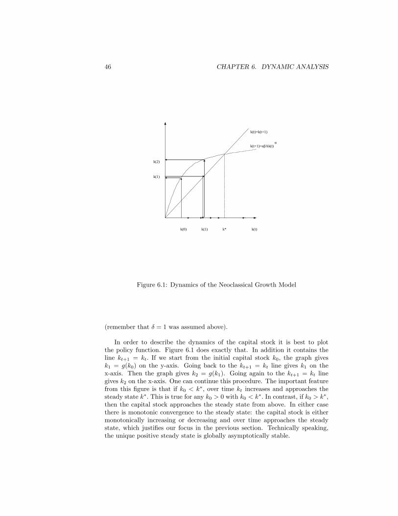
Figure 6.1: Dynamics of the Neoclassical Growth Model

(remember that � = 1 was assumed above).

In order to describe the dynamics of the capital stock it is best to plotthe policy function. Figure 6.1 does exactly that. In addition it contains theline kt+1 = kt: If we start from the initial capital stock k0; the graph givesk1 = g(k0) on the y-axis. Going back to the kt+1 = kt line gives k1 on thex-axis. Then the graph gives k2 = g(k1). Going again to the kt+1 = kt linegives k2 on the x-axis. One can continue this procedure. The important featurefrom this �gure is that if k0 < k�; over time kt increases and approaches thesteady state k�: This is true for any k0 > 0 with k0 < k�: In contrast, if k0 > k�;then the capital stock approaches the steady state from above. In either casethere is monotonic convergence to the steady state: the capital stock is eithermonotonically increasing or decreasing and over time approaches the steadystate, which justi�es our focus in the previous section. Technically speaking,the unique positive steady state is globally asymptotically stable.

6.2. LINEARIZATION OF THE EULER EQUATION 47

6.2 Linearization of the Euler Equation

In general the Euler equation is not a linear equation, and thus we can�t easilysolve it. But what we can do is to make the Euler equation linear by approximat-ing the nonlinear equation linearly around its steady state. Roughly speakingthis is nothing else but doing a Taylor series approximation around the steadystate of the model, which we have solved before. The resulting approximatedEuler equation is linear, and hence easy to solve for the policy function g ofinterest. Keep in mind, however, that we only solve for an approximate solution(unless of course we assume quadratic utility and linear production, as above).While there are numerical methods to solve for the exact nonlinear solution,these are not easy to implement and thus not discussed in this class.Let c�; k�; y� denote the steady state values of consumption, capital and

output. We have already discussed above how to �nd this steady state. Theidea is to replace the nonlinear Euler equation

u0(ct) = �u0(ct+1)��Ak��1t+1 + (1� �)

�(6.3)

where

ct = Ak�t � kt+1 + (1� �)ktct+1 = Ak�t+1 � kt+2 + (1� �)kt+1

with a linear version, because linear equations are much easier to solve.

6.2.1 Preliminaries

There is one crucial tool for turning the nonlinear Euler equation into a linearequation: Taylor�s theorem. This theorem states that we can approximate afunction f(x) around a point a by writing

f(x) = f(a) + f 0(a)(x� a) + 12f 00(a)(x� a)2 + 1

6f 000(a)(x� a)3 + : : :

Note that the approximation is only exact by using an in�nite number of terms.But in order to make a nonlinear equation into a linear equation we will use theapproximation

f(x) � f(a) + f 0(a)(x� a) (6.4)

and hope we will not make too big of an error. Note however that for all x 6= awe will make an error; how severe this error is depends on the application andcan only exactly be answered for examples in which we know the true solution.In our application we will use as point of approximation a the steady state ofthe economy. As long as the economy does not move too far away from thesteady state, we can hope that the approximation in (6:4) is accurate.Similarly, for a function of two variables we have

f(x; y) � f(a; b) +@f(a; b)

@x(x� a) + @f(a; b)

@y(y � b) (6.5)


Finally, often researchers prefer to express deviations of a variable xt from itssteady state x� not in its deviation (xt � x�); but in its percentage deviationxt =

xt�x�xt

; since this is easier to interpret. For future reference note that

log(xt)� log(x�) = log� xtx�

�= log

�xt � x�x�

+ 1

�� xt =

xt � x�x�

Also for future reference note that

xt � x� =xt � x�x�

x� = xtx�

We will use these facts repeatedly below.

6.2.2 Doing the Linearization

We want to linearize

u0(ct) = �u0(ct+1)��Ak��1t+1 + (1� �)

�where (6.6)

ct = Ak�t � kt+1 + (1� �)kt (6.7)

ct+1 = Ak�t+1 � kt+2 + (1� �)kt+1 (6.8)

Let�s do this slowly for the �rst time, since this procedure is prone to makingmistakes (believe me, I know what I am talking about). We start with equation(6:7); which can be rewritten as

0 = Ak�t � kt+1 + (1� �)kt � ct (6.9)

Let us do term by term. First, let�s linearize the term Ak�t around the steadystate k�: This yields, using (6:4);

Ak�t � A (k�)�+ �A (k�)

��1 � (kt � k�)= A (k�)

�+ �A (k�)

��1 � k�kt= A (k�)

�+ �A (k�)

�kt

Note that the only variable here is kt; since k� is the steady state capital stock,and hence a �xed number, and the rest is just a bunch of parameters. Nowconsider the term �kt+1; again using (6:4) we get

�kt+1 � �k� � (kt+1 � k�) = �k� � k�kt+1

where in this case the linear approximation is exact, since the function f(kt+1) =�kt+1 is linear to start with. Similarly

(1� �)kt � (1� �)k� + (1� �)k�kt�ct � �c� � c�ct


and thus the linear approximation of (6:9) reads as

0 � A (k�)�+ �A (k�)

�kt � k� � k�kt+1 + (1� �)k� + (1� �)k�kt � c� � c�ct

= A (k�)� � k� + (1� �)k� � c� + �A (k�)� kt � k�kt+1 + (1� �)k�kt � c�ct:

(6.10)

Finally realize that, at the steady state (c�; k�), the resource constraint (6:9)holds. Thus we can simplify (6:10) to (replacing the � with an equality sign)

0 � �A (k�)�kt � k�kt+1 + (1� �)k�kt � c�ct

c�ct = �A (k�)�kt � k�kt+1 + (1� �)k�kt

=h�A (k�)

��1+ (1� �)

ik�kt � k�kt+1 (6.11)

which is a linear equation with the three variables (ct; kt; kt+1): Using exactlythe same logic we can linearize (6:8) to obtain

c�ct+1 = �A (k�)�kt+1 � k�kt+2 + (1� �)k�kt+1

=h�A (k�)

��1+ (1� �)

ik�kt+1 � k�kt+2 (6.12)

The really painful equation is equation (6:6)

0 = �u0(ct) + �u0(ct+1)��Ak��1t+1 + (1� �)

�= �u0(ct) + (1� �)�u0(ct+1) + �u0(ct+1)�Ak��1t+1 (6.13)

Again proceeding term by term we have, using (6:4);

�u0(ct) � �u0(c�)� u00(c�)(ct � c�)= �u0(c�)� u00(c�)c�ct

and(1� �)�u0(ct+1) = (1� �)�u0(c�) + (1� �)�u00(c�)c�ct+1

The last term is more complicated, since it involves a function of two variables,(ct+1; kt+1): Using (6:5) we have

�u0(ct+1)�Ak��1t+1

� �u0(c�)�A (k�)��1

+ �u00(c�)�A (k�)��1

(ct+1 � c�) + �u0(c�)�(�� 1)A (k�)��2 (kt+1 � k�)= �u0(c�)�A (k�)

��1+ �u00(c�)�A (k�)

��1c�ct+1 + �u

0(c�)�(�� 1)A (k�)��1 kt+1

Inserting all terms into (6:13) and re-grouping yields

0 = �u0(c�) + (1� �)�u0(c�) + �u0(c�)�A (k�)��1

�u00(c�)c�ct + (1� �)�u00(c�)c�ct+1 + �u00(c�)�A (k�)��1 c�ct+1 + �u0(c�)�(�� 1)A (k�)��1 kt+1


But the entire �rst line of this expression equals zero, since equation (6:13) holdsin the steady state (ct = ct+1 = c�; kt+1 = k�): Thus the linearized version ofequation (6:13) becomes

u00(c�)c�ct = (1� �)�u00(c�)c�ct+1 + �u00(c�)�A (k�)��1 c�ct+1 + �u0(c�)�(�� 1)A (k�)��1 kt+1=

h(1� �) + �A (k�)��1

i�u00(c�)c�ct+1 + �u

0(c�)�(�� 1)A (k�)��1 kt+1 (6.14)

which is again a linear function in (ct; ct+1; kt+1): Arguably the system of equa-tions (6:6); (6:7) and (6:8) is a mess, but it is a linear mess. Inserting (6:6) and(6:7) into (6:8) yields

u00(c�)nh�A (k�)

��1+ (1� �)

ik�kt � k�kt+1

o=

h(1� �) + �A (k�)��1

i�u00(c�) �nh

�A (k�)��1

+ (1� �)ik�kt+1 � k�kt+2

o+�u0(c�)�(�� 1)A (k�)��1 kt+1

Collecting terms yieldsnu00(c�)

h�A (k�)

��1+ (1� �)

iok�kt

�(

u00(c�)k� +h(1� �) + �A (k�)��1

i�u00(c�)

h�A (k�)

��1+ (1� �)

ik�

+�u0(c�)�(�� 1)A (k�)��1

)kt+1

+h(1� �) + �A (k�)��1

i�u00(c�)k�kt+2

= 0

orc1kt + c2kt+1 + c3kt+2 = 0 (6.15)

where the three constants (c1; c2; c3) are given by

c1 = u00(c�)k�=� < 0

c2 = �nu00(c�)k� + u00(c�)k�=� + �u0(c�)�(�� 1)A (k�)��1

o> 0

c3 = u00(c�)k� < 0

since in the steady stateh(1� �) + �A (k�)��1

i� = 1: The nice thing about

equation (6:15) is that this, in contrast to (6:3); is a linear second order di¤erenceequation, which we know very well how to solve.Again, what we are looking for is a policy function giving kt+1 = g(kt): Let

us again guess that this function takes the form

kt+1 = g(kt) = skt and thus

kt+2 = skt+1 = s2kt


where s is a constant to be determined. Inserting the guessed policy functioninto equation (6:15) yields2

c1kt + c2skt + c3s2kt = 0 or

c1 + c2s+ c3s2 = 0

s2 +c2c3s+

c1c3

= 0

s2 � 1s+ 2 = 0

where

2 =c1c3=1

�

1 = �c2c3= 1 +

1

�+�u0(c�)�(�� 1)A (k�)��1

u00(c�)k�

This is simply a quadratic equation in s with the two solutions

s1;2 = 12�� 214� 2

� 12

There are some good news here. First we note that, since

1 > 2 + 1 (6.16)

we have that

214� 2 >

1

4(1 + 2)

2 � 2 =1

4

h(1 + 2)

2 � 4 2i=1

4(1� 2)

2 � 0 (6.17)

and thus both roots are real. Second we note that

s1 � s2 = 214� 214+ 2 =

1

�

and since 1 > 0 we know that both roots are positive. The bigger root satis�es,using (6:16) and (6:17)

s1 = 12+

� 214� 2

� 12

> 12+1

2( 2 � 1) =

1 + 2 � 12

>2 22= 2 =

1

�

and thus the smaller root satis�es

s2 = 12�� 214� 2

� 12

< 1:

2The procedure of parameterizing the policy function by a coe¢ cient s and then solvingfor it is sometimes called the method of undetermined coe¢ cients.


What have we accomplished? We guessed that the optimal policy functionsatis�ed

kt+1 = skt

and found that such a function indeed satis�es the log-linearized version of theEuler equation, as long as either s = s1 or s = s2: But what is the right choiceof s? Remember that

kt =kt � k�k�

and thus

kt = (1 + kt)k�:

Also remember that we are dealing with the case T = 1: Therefore we onlyhave the initial condition k0 given, but no terminal condition. Now supposethat we select s1 > 1 and suppose k0 < k�; so that k0 < 0; that is we start withour capital stock below the steady state. But our policy function tells us

k1 = s1k0

k2 = s1k1 = s21k0 and in general

kt = st1k0 (6.18)

Since s1 > 1; as t gets larger and larger, st1 grows exponentially towards in�nity.Consequently kt becomes more and more negative. At some point in time wehave kt < �1; and thus

kt = (1 + kt)k� < 0 (6.19)

which can never be optimal. A similar argument shows that if the economystarts with k0 > k� and thus k0 > 0; then kt ! 1 as time goes to in�nity.Thus kt increases over time (kt+1 > kt) and kt !1 with time. But again thiscannot be optimal since

ct = Ak�t + (1� �)kt � kt+1 < Ak�t � �kt < 0

if kt >�A�

� 11�� ; which happens for large enough t (as long as � < 1). It can

simply not be optimal to drive the capital stock to in�nity, since at some pointsimply replacing the depreciated capital requires all of current production, andnothing is left for consumption. Thus with s = s1 the capital stock eitherbecomes negative or explodes over time which cannot be the optimal policy ofthe social planner. Therefore we can discard this root, and focus on the otherroot s2 2 (0; 1): For this root we have that st1 ! 0 as t becomes large. Thusfrom (6:18) we see that kt goes to 0 over time, and from (6:19) we see thatkt converges to the steady state k� over time. Since the optimal policy of thelinearized problem is

kt+1 = skt

with s 2 fs1; s2g and we have discarded the case s = s1; our optimal policy is

kt+1 = s2kt


where s2 2 (0; 1) is a �xed number that of course depends on the parametervalues of the economy. The dynamics of the capital stock of the economy (andthus output, consumption and the like) is described as monotonic convergence tothe steady state, from above if k0 > k� and from below if k0 < k�: It looks verymuch like the dynamics in �gure 6:1; with the di¤erence that the policy functionin the �gure was nonlinear, whereas now it is linear (in percentage deviations).The root s1 is sometimes called the unstable root, because it leads the capitalstock to explode or implode. The root s2 is called the stable root, since it leadsto monotonic convergence to the steady state. A situation where both roots arereal and exactly one is stable is a very desirable situation, because then we haveone, and only one, optimal policy function. The neoclassical growth model hasthis desired property.Two �nal remarks. First, note that the policy function is linear in percentage

deviations from the steady state. Of course it is easy to derive the policy functionin capital levels. We have

kt+1 = s2kt (6.20)kt+1 � k�

k�= s2 �

kt � k�k�

kt+1 � k� = s2 (kt � k�)kt+1 = (1� s2)k� + s2kt (6.21)

Second, I again want to stress that the so-derived policy function is only anapproximation to the true policy function. We can see this from the example inthe last section where we derived the true policy function as

kt+1 = ��Ak�t (6.22)

Whatever the value for s2 is (of course we can calculate it, it is a messy functionof the parameters of the model), the approximation in (6:21) is not equal to thetrue policy function (6:22); unless of course we are in the steady state: kt = k�:

Note however, since kt � log(kt)� log(k�), we have from (6:20)

log(kt+1) � (1� s2) log(k�) + s2 log(kt):

On the other hand, taking logs of (6:22) yields

log(kt+1) = log (��A) + � log(kt):

Thus, for the particular example our linear (in percentage deviations from thesteady state) approximation is very accurate; in fact the only approximation(which we know is very good for small deviations from steady state) is due tothe fact that

kt � k�k�

� log(kt)� log(k�)

Thus for the parameterization in the previous section (� = 1; u(c) = log(c)), wewould expect s2 = �: It is a useful exercise to verify this.


Obviously all other variables of interest (consumption c; output y and in-vestment i) can be easily computed once we know capital. For this one caneither use the exact equations, e.g.

ct = Ak�t + (1� �)kt � kt+1or the linear approximation, if one prefers this

c�ct =h�A (k�)

��1+ (1� �)

ik�kt � k�kt+1:

6.3 Analysis of the Results

6.3.1 Plotting the Policy Function

One way to represent the results from the previous section is to simply plotkt+1 = g(kt) against kt as in �gure 6:1: Usually the dynamics of the capitalstock can be deduced from such a plot already fairly completely, at least in amodel without stochastic shocks as we have discussed so far.

6.3.2 Impulse Response Functions

The idea of an impulse response function is to plot what happens to our variablesof interest in response to an exogenous shock to the economy, conditional on theeconomy being in the steady state before the shock. While in a model withoutstochastic shocks this is a bid strange, one can still do it. Suppose that theeconomy at time t = 0 is in the steady state (k0 = k�; k0 = 0), and then at thebeginning of period 1 for some reason the capital stock gets reduced by 1% (aterroristic attack, say). We can use the policy function kt+1 = g(kt) to deducewhat happens to the capital stock over time:

k0 = 0; k0 = k�

k1 = �0:01; k1 = 0:99k�

k2 = �0:01s2; k2 = (1� 0:01s2)k� and in generalkt = �0:01st�12 ; kt = (1� 0:01st�12 )k�

A plot of the sequence fktgTt=0 or fktgTt=0 is called an impulse response function,because it plots the response of the capital stock to the initial impulse of a shockover time. Obviously we can do exactly the same with the policy function ofthe nonlinear problem, if we can possibly solve it.Figure 6.2 plots an impulse response function for capital. The impulse is a

1% reduction of the capital stock, and the policy function used is kt+1 = 0:333kt:We observe the quick convergence of the model back to its steady state.

6.3.3 Simulations

In a deterministic model (i.e. a model without stochastic shocks) a simulationis something very similar to an impulse response. In a stochastic model the

6.3. ANALYSIS OF THE RESULTS 55

0 2 4 6 8 10

1

0.8

0.6

0.4

0.2

0

Time

Perc

enta

ge D

evia

tion

from

Ste

ady

Stat

e

Impulse Response for Capital

Figure 6.2: Impulse Response Function for Capital

di¤erence between the two ways to analyze the results of the model will bemore di¤erent. In a simulation one picks some initial condition of the economy,k0; and then uses the policy function g to simulate a long sequence of capitalstocks according to kt+1 = g(kt); that is

k1 = g(k0)

k2 = g(k1)

and so forth. Of course one can again plot the sequence fktg against time.Alternatively, one can compute statistics of interest of these arti�cial data (forexample the standard deviation, autocorrelation and so forth). In order toassess how good the model performs empirically one can then compare thestatistics derived from the arti�cial model data to the statistics computed fromreal data. We do exactly this when taking our model (with stochastic shocks)to the business cycle data.


6.4 Summary

The previous discussion about the linearization approach was very detailed, soit is worth summarizing the main steps involved.

1. Obtain the equations characterizing socially optimal (equivalently, equi-librium allocations)

2. Linearize them

3. Guess a linear policy function and solve for the undetermined coe¢ cientsof this policy function

4. Analyze the results by plotting the policy functions, impulse responses,simulations and compute statistics of the arti�cial data generated by themodel. Finally compare them to real data.

5. Interpret the results.

This sounds very involved, but the nice thing is that a lot of these stepscan be carried out by a computer, since they are purely mechanical. What ismore, there now exists pre-programed software that does it for you, so you don�thave to do it by yourself. The toolkit by Harald Uhlig that Philip is and willbe using in the Tutorials is such freely available software. What still requireshuman work, however, are steps 1.,2. and 5. The painful step 2. of linearizingthe equations will hopefully be somewhat automated soon, but so far you stillhave to do it by yourself.

Chapter 7

A Note on EconomicGrowth

So far the model we described does not display long-run growth, since the econ-omy converges to its steady state. The data, in contrast, shows long-run growthat a positive rate. Part of this growth in the data is due to population growth,but even GDP per capita grows at a positive rate per capita. While long-rungrowth is not our main interest, it still would be nice if our model is consistentwith the long-run growth observations as well. Fortunately this is quite easy toachieve.

7.1 Preliminary Assumptions and De�nitions

Assume that the population and labor force grows at constant net growth raten; so that the number of workers is given by

nt = (1 + n)tn0

= (1 + n)t

where n0 = 1 is the size of the labor force at period 0: Furthermore assume thatthe production function is given by

Yt = AK�t

�(1 + g)tnt

�1��where g is the growth rate of technological, labor augmenting progress. Thusthe aggregate resource constraint is given by

Ct +Kt+1 � (1� �)Kt = AK�t

�(1 + g)tnt

�1��I used capital letters for output and capital now, since now it is important todistinguish between aggregate and per capita variables. All aggregate variableswill now be growing because of population growth and technical progress; thus

57

58 CHAPTER 7. A NOTE ON ECONOMIC GROWTH

our aim is to reformulate the economy in terms of variables that are, at leastpotentially, constant over time.Thus a few tedious, but useful de�nitions: let

ct =Ct

(1 + n)t

yt =Yt

(1 + n)t

kt =Kt

(1 + n)t

denote per capita variables and

~ct =Ct

(1 + n)t(1 + g)t=

ct(1 + g)t

~yt =Yt

(1 + n)t(1 + g)t=

yt(1 + g)t

~kt =Kt

(1 + n)t(1 + g)t=

kt(1 + g)t

denote variables per e¤ective unit of labor.The social planner problem is now given by

maxfct;kt+1gTt=0

TXt=0

�tu(ct)

subject to

Ct +Kt+1 � (1� �)Kt = AK�t

�(1 + g)tnt

�1��ct � 0 and K0 > 0 given

7.2 Reformulation of Problem in E¢ ciency Units

We want to rewrite this problem in terms of variables that are not constantlygrowing over time, that is, in terms of the ~ variables. First note that K0 =k0 = ~k0; since (1 + n)0 = (1 + g)0 = 1: Second, ct � 0 if and only if ~ct � 0; sothe only two things we have to worry about are the resource constraint and theutility function.Divide the resource constraint by (1 + n)t(1 + g)t to obtain

Ct(1 + n)t(1 + g)t

+Kt+1

(1 + n)t(1 + g)t� (1� �)Kt

(1 + n)t(1 + g)t=AK�

t ((1 + g)tnt)

1��

(1 + n)t(1 + g)t

and, using the variable de�nitions

~ct +Kt+1

(1 + n)t(1 + g)t� (1� �)~kt =

AK�t ((1 + g)

tnt)1��

(1 + n)t(1 + g)t:

7.2. REFORMULATION OF PROBLEM IN EFFICIENCY UNITS 59

But now note that

Kt+1

(1 + n)t(1 + g)t=

Kt+1

(1 + n)t+1(1 + g)t+1� (1 + g)(1 + n) = (1 + g)(1 + n)~kt+1

AK�t ((1 + g)

tnt)1��

(1 + n)t(1 + g)t= A

K�t

[(1 + n)t(1 + g)t]� �

((1 + g)tnt)1��

[(1 + n)t(1 + g)t]1�� = A~k�t

and thus the resource constraint becomes

~ct + (1 + g)(1 + n)~kt+1 � (1� �)~kt = A~k�t :

Finally let us work on the lifetime utility function. Assume that the periodutility function of the constant relative risk aversion form

u(c) =c1��

1� �

where � is a parameter.1 If � = 1; we take the utility function to be u(c) =log(c): Note that with this utility function we have that

u(ct) =c1��t

1� � =(~ct(1 + g)

t)1��

1� � = (1 + g)t(1��)~ct1��

1� �

Thus we can rewrite the lifetime utility function of the representative family as

TXt=0

�tu(ct) =

TXt=0

�t(1 + g)t(1��)u(~ct)

=TXt=0

~�tu(~ct)

where ~� = �(1 + g)1��:After all the smoke has settled, the social planner problem is given by

maxfct;kt+1gTt=0

TXt=0

~�tu(~ct)

subject to

~ct + (1 + g)(1 + n)~kt+1 � (1� �)~kt = A~k�t

~ct � 0 and ~k0 > 0 given

1Note that the paramter � is equal to the coe¢ cient of relative risk aversion:

�cu00(c)u0(c)

= �

and thus measures how risk averse the household is. The higher �; the higher is the riskaversion of the household.


7.3 Analysis

Again forming the Lagrangian

L =TXt=0

~�tu(~ct) +

TXt=0

�t

�A~k�t � ~ct � (1 + g)(1 + n)~kt+1 + (1� �)~kt

�= : : :+ ~�

tu(~ct) + ~�

t+1u(~ct+1) + : : :

+�t

�A~k�t � ~ct � (1 + g)(1 + n)~kt+1 + (1� �)~kt

�+�t+1

�A~k�t+1 � ~ct+1 � (1 + g)(1 + n)~kt+2 + (1� �)~kt+1

�+ : : :

Taking �rst order conditions with respect to ~ct; ~ct+1 and ~kt+1 yields

~�tu0(~ct) = �t

~�t+1

u0(~ct+1) = �t+1

(1 + g)(1 + n)�t = �t+1

��A~k��1t+1 + (1� �)

�Dividing the second equation by the �rst yields

�t+1�t

=~�u0(~ct+1)

u0(~ct)

From the third equation we have

�t+1�t

=(1 + g)(1 + n)�

�A~k��1t+1 + (1� �)�

and thus combining the two yields

~�u0(~ct+1)

u0(~ct)=

(1 + g)(1 + n)��A~k��1t+1 + (1� �)

�~�u0(~ct+1)

��A~k��1t+1 + (1� �)

�(1 + g)(1 + n)

= u0(~ct) (7.1)

which is almost exactly the Euler equation we found when abstracting from pop-ulation and productivity growth, with the exception that the marginal productof capital has to be divided by (1 + g)(1 + n):

7.4 The Balanced Growth Path

We can repeat exactly the same analysis of a steady state in the model withgrowth. But if ~ct is constant over time, per capita consumption ct = ~ct(1 + g)t

7.4. THE BALANCED GROWTH PATH 61

grows at constant rate g; thus such a situation is not called a steady state, buta balanced growth path (since all per capita variables grow at constant rates).Now let us characterize the balanced growth path. Since ~ct = ~ct+1; the balancedgrowth path e¤ective capital stock ~k� satis�es

~�

��A~k��1 + (1� �)

�(1 + g)(1 + n)

= 1

or

(1 + g)1��A~k��1 + (1� �)

�(1 + �)(1 + g)(1 + n)

= 1

~k� =

�(1 + �)(1 + g)(1 + n)(1 + g)��1 � (1� �)

�A

� 1��1

=

��A

(1 + �)(1 + g)(1 + n)(1 + g)��1 � (1� �)

� 11��

Note that if the period function is logarithmic, that is � = 1; and the terms�g; �n; gn and �ng are su¢ ciently small (which is the case as long as �; n; g aresmall), then

~k� =

��A

�+ g + n+ �)

� 11��

which is as before, only that the physical depreciation rate � has to be augmentedby the population growth rate and the growth rate of technological progress.From the resource constraint e¤ective consumption is given by

~c� = A~k�t � (1 + g)(1 + n)~kt+1 + (1� �)~kt= A

�~k�� [(1 + g)(1 + n)� (1� �)] ~k�

� A�~k�� [g + n+ �] ~k�

and e¤ective output in the balanced growth path is given by

~y� = A�~k��

which in the log-utility case equals

y� = A

��A

�+ g + n+ �

� �1��

= A1

1��

��

�+ g + n+ �

� �1��

(7.2)

As discussed before, all per-capita variables grow at constant rate g in thebalanced growth path, and all aggregate variables at rate n+ g (approximately,using (1 + n)(1 + g) � 1 + n + g). How about wages and interest rates, alongthe balanced growth path?


As before, the representative �rm solves the maximization

maxAK�t

�(1 + g)tnt

�1�� wtnt � (rt � �)Kt

where Nt and Kt is the number of workers and capital the �rm hires. The �rstolder conditions read as

wt = (1� �)(1 + g)tA�

Kt

(1 + g)tnt

��= (1� �)(1 + g)tA

�~kt

��rt = �A

�Kt

(1 + g)tnt

��1� � = �A

�~kt

��1� �

Along the balanced growth path ~kt is constant, and thus the real interest ratert is constant and the real wage wt is growing at a constant rate g:To summarize, with economic growth it is as easy, or as hard, to solve this

model that without growth. The presence of economic growth a¤ects, however,the choice of the parameter values. How to pick these parameter values indiscussed next.

Chapter 8

Calibration

Let us �rst collect all the parameters of the model. There are three sets ofparameters we need to choose

� Technology parameters: (A;�; �; g)

� Demographic parameters: (n)

� Preference Parameters: (�; �)

The process of choosing these parameters is often called calibration. Theidea is the following: we want to make the model�s predictions to match cer-tain observations from the data. Since we are interested in the business cycleproperties of the model and do not want to cheat by choosing parameter valuesthat help the model deliver good business cycle implications, we rather chooseparameter values such that the long run implications of the model matches longrun average observations from the data. Obviously the long run facts di¤er bycountries. I will present a choice of parameter values calibrated to US data.It is interesting, and a good start for a diploma thesis, to do exactly the sameanalysis for other countries as well.First we have to choose the length of a period, since our growth rates, for

example, refer to growth rates from one period to the next. Therefore it isobviously crucial to specify how long a period lasts. Since most of business cycleresearch is done with quarterly data, we will use as period length a quarter.

8.1 Long Run Growth Rates

In the model n equals the growth rate of the population, which equals the growthrate of the labor force in the model as well. The annual average populationgrowth rate in the US is about 1:1% per year. Thus the quarterly growth rate

63

64 CHAPTER 8. CALIBRATION

of the population (labor force) solves

(1 + n)4= 1:011 or

n = (1:011)14 � 1 � 0:27%

We follow the same logic for the growth rate of technology g; which gives thegrowth rate of output per capita (per worker or per hour worked, all the samein the model). Between 1947 and 2004 the average growth rate of GDP percapita was 2:2% per year, and thus

(1 + g)4 = 1:022 or

g = (1:022)14 � 1 � 0:55%

8.2 Capital and Labor Share

We saw above that the production function parameter � equals the capital sharein the model. Thus we want to choose a value for � that corresponds to thelong run capital share in the data. At �rst this seems straightforward to do,until one realizes that it is not completely obvious how to compute the laborshare and capital share in the data. One important problem is proprietor�sincome, that is, the income that people earn that own and run their business,supplying both their labor and their capital to the business. Another problemis the imputation of rental income for owner-occupied housing. If you own thehouse you live in, conceptually the rent that you should charge yourself for yourhome should count as capital income (since the rent a landlord gets from hertenants counts as capital income). In practice the statistics often do not capturethis.Without going into the dirty details we choose as compromise a � = 1

3 ;re�ecting a long-run labor share in the data of roughly 2

3 : The range of estimatesused in the literature (at least the one I am aware of) is � 2 [0:25; 0:4]:

8.3 The Depreciation Rate

Output is divided between consumption and investment. In the BGP investmentequals ~{� = [g + n+ �] ~k�: Thus the investment share of output equals

I

Y=

~{�

~y�= (g + n+ �)

~k�

~y�= (g + n+ �)

K

Yand thus

(g + n+ �) =I=Y

K=Y

� =I=Y

K=Y� n� g

Thus with long-run averages for the investment-output ratio and the capital-output ratio from the data we can pin down �: In US data the investment-output

8.4. THE TECHNOLOGY CONSTANT A 65

share is roughly 25% in the long run, and the capital-output ratio is roughly2:6 on an annual level. Note that the capital stock is a stock, and thus refersto a variable at a point in time. In contrast, output and investment are �owvariables, and refer to a period of time (and thus depend on the period length).Thus if the annual capital-output ratio is 2:6; the quarterly ratio is 2:6�4 = 10:4;re�ecting the fact that quarterly GDP is one forth of annual GDP.Thus we have as quarterly depreciation rate

� =0:25

10:4� 0:0027� 0:0055 = 1:6%

Here we also see the importance of incorporating or ignoring growth in themodel: abstracting from growth we would have chosen a depreciation rate of� = 2:42% per quarter.

8.4 The Technology Constant A

The choice of A simply pins down the unit of measurement. Doubling A simplydoubles all economic variables, without changing anything else. Often econo-mists set A = 1 or set A such that steady state output ~y = 1 (conditional onall other parameters this is easily done using (7:2)). But it is a good check ofyour answers to questions (or your computer code) that indeed A is simply anormalization, and multiplying it by some number should multiply all economicvariables by the same number (apart from ratios of variables and the interestrate, of course, which should remain unchanged).

8.5 Preference Parameters

The crucial equation for choosing preference parameters is the Euler equation(7:1)

~�u0(~ct+1)

��A~k��1t+1 + (1� �)

�(1 + g)(1 + n)

= u0(~ct)

which in the BGP becomes

~�

��A~k��1t+1 + (1� �)

�(1 + g)(1 + n)

= 1

Using the fact that the real interest rate equals the marginal product of capitalnet of depreciation, this becomes

~�1 + r�

(1 + g)(1 + n)= 1 or

�(1 + g)1�� (1 + r�)

(1 + g)(1 + n)= 1 or

1 + r� = (1 + g)(1 + n)(1 + �)(1 + g)��1

66 CHAPTER 8. CALIBRATION

Parameter A � � � �g = 0; n = 0 1 0:33 2:42% 1 1%

g = 0:55%; n = 0 1 0:33 1:87% 1 0:45%g = 0:55%; n = 0:27% 1 0:33 1:6% 1 0:2%

Table 8.1: Parameter Values

The parameter � is hard to pin down using long-run observations, so economistsoften pick it independently. The preferred choice is � = 1; that is logarithmicutility, in which case

1 + r� = (1 + g)(1 + n)(1 + �)

Finally, the time discount rate is chosen such that, conditional on the choicesfor g and n; the balanced growth path of the model has an interest rate thatmatches its long run average in the data. Of course there are many real interestrates in the data, and the real interest rate in the model is both the risk-freereal interest rate as well as the real return on capital. The former has an annualaverage of about 1%; the latter of about 7� 8%: As a compromise we target anr� of 4% per annum, or 1% quarterly. Conditional on the values of g; n chosenabove this yields � = 0:002 = 0:2% quarterly. Again note that when calibratingan economy without growth, one would choose a � = 1% quarterly.

8.6 Summary

The following Table 8.1 summarizes the common choice of parameters for themodel, both when calibrating a model without and with growth. The periodlength is a quarter.

Chapter 9

Adding Labor Supply

Now we could in principle simulate the economy, compute impulse responsesor any other statistic that characterizes the equilibrium of the model. Beforethat we have to address two shortcomings, however. First, as we saw in thedata section, the amount of labor used in production varies with the businesscycle. In fact, apart from GDP (growth) itself, the unemployment rate is pos-sibly the most important indicator of the business cycle, with high employmentcharacterizing booms and low employment (high unemployment) characterizingrecessions. Therefore in this section we now give households the opportunity toadjust their labor supply. Second, and this will be done in the next subsectionwe will introduce technology shocks that will make our economy to actually dis-play business cycles. The endogenous response of employment to these shockswill then amplify the e¤ects of these shocks on GDP.In the standard real business cycle model the labor market is modelled as

completely frictionless spot market where workers are paid their marginal prod-uct as wage. This wage clears the labor market, and thus at the market wageeveryone that wants to work can do. There is no involuntary unemployment(whatever that means), but certainly households that do not �nd it preferableto work may choose not to supply any labor. Thus in no sense do we rule outunemployment (or better, non-employment).

9.1 The Modi�ed Social Planner Problem

Lifetime preferences of the representative household become

TXt=0

�t [u(ct)� lt]

where lt 2 [0; 1] is the total number of hours the household works. We normalizethe total time the household has available in a given period to 1. The number is a parameter and determines how painful it is for a household to work,

67

68 CHAPTER 9. ADDING LABOR SUPPLY

with higher implying higher disutility from work. The parameter can alsobe interpreted as the marginal utility of leisure.1 The social planner problembecomes2

maxfct;kt+1;ltgTt=0

TXt=0

�t [u(ct)� lt] (9.1)

subject to

ct + kt+1 � (1� �)kt = Ak�t l1��t

ct � 0; lt 2 [0; 1] and k0 > 0 given

The speci�cation of disutility of labor is peculiar, but, as we will see, necessaryto get good business cycle results. It is linear in the disutility of labor, whichwill imply that labor supply reacts quite strongly to changes in wages. Sinceempirically labor input is quite volatile over the business cycle we will need everyhelp we can get to make it volatile in the model as well. A strong response oflabor supply to hours is therefore desirable.

9.2 Labor Lotteries

But how can we justify that the marginal disutility of labor is constant at ,whereas the marginal utility of consumption is strictly decreasing (rememberthat u00 < 0 was assumed)? Here is a trick that goes back to Richard Roger-son (Journal of Monetary Economics, 1988), one of Ed Prescott�s most famousstudents. Suppose that the utility function is given by

TXt=0

�t [u(ct)� v(lt)]

where the function v satis�es v0 > 0 and v00 > 0: That is, working more reducesutility, and the more you work the more hurts an additional hour of work.Assume that households can either work full time, lt = 1 or not at all, lt = 0;

1The restriction to at most one unit of work is a simple normalization. Suppose a householdcan supply at most h hours of work and the utility from leisure h� l is given by

(h� l)

then (h� l) = h� l:

But since h is simply a constant and adding constants to the utility function does not changethe optimal labor (or consumption) choice, both formulation of the utility function give exactlythe same outcomes.

2For simplicity we abstract from technology and population growth here. If the populationis growing and there is technological progress we have exactly the same problem, but theproduction function would read as

AK�t

�(1 + g)tntlt

�1��

9.3. ANALYZING THE MODEL WITH LABOR 69

that is, they either have a job or they don�t. Now assume that the socialplanner (or some unemployment agency) provides full insurance against beingunemployed: no matter whether employed or unemployed, you receive the sameamount of consumption. For this to work obviously it cannot be possible foragents to shirk unobservably, otherwise all people would claim to not be able to�nd a job (because they don�t like to work and still get the same consumptioneven if they don�t work). Finally denote by �t the fraction of the populationthat the planner chooses to work (that is, �t is a choice variable of the socialplanner) and by ct the consumption level that both employed and unemployedget. Finally assume that all people get picked to work the same probability, so�t is also the probability that a particular agent gets picked (remember we havea big number of identical agents of total number equal to 1). What the plannere¤ectively does is to play a labor lottery with full consumption insurance.Then expected utility in the current period is given as

E fu(ct)� v(lt)g = �t [u(ct)� v(lt = 1)] + (1� �t) [u(ct)� v(lt = 0)]= u(ct)� �t [v(1)� v(0)]� v(0)

But note that since v(1); v(0) are just two numbers and we can always ignoreconstants added to the utility function (they don�t change �rst order conditionsand thus optimal choices), we can rewrite the e¤ective utility function as

E fu(ct)� v(lt)g = u(ct)� �t

where = [v(1)� v(0)] > 0 and we simply dropped the constant �v(0): Re-placing the name of the choice variable �t by lt gives back our original utilityfunction. Also note that in the production function total labor input is equalto the fraction of workers working, �t times their time worked (= 1); so totallabor input equals �t = lt: Thus the assumption of labor lotteries plus perfectconsumption insurance justi�es the usage of the particular functional form ofdisutility of labor in the utility function. Below we will describe how one canobtain the same result in a competitive market situation. But �rst we wantto analyze the optimality conditions of the social planner problem with laborsupply.

9.3 Analyzing the Model with Labor

Writing down the Lagrangian and ignoring the inequality constraints yields

L =TXt=0

�t [u(ct)� lt] +TXt=0

�t�Ak�t l

1��t + (1� �)kt � ct � kt+1

�= : : : �t [u(ct)� lt] + �t

�Ak�t l

1��t + (1� �)kt � ct � kt+1

�+

�t+1 [u(ct+1)� lt+1] + �t+1�Ak�t+1l

1��t+1 + (1� �)kt+1 � ct+1 � kt+2

�+ : : :


Taking �rst order conditions with respect to ct; lt; ct+1; kt+1 and setting to zeroyields

�tu0(ct) = �t (9.2)

�t(1� �)A�ktlt

��= �t (9.3)

�t+1u0(ct+1) = �t+1 (9.4)

�t = �t+1

"�A

�lt+1kt+1

�1��+ (1� �)

#(9.5)

Combining equations (9:2); (9:4) and (9:5) yields the familiar intertemporalEuler equation

u0(ct) = �u0(ct+1)

"�A

�lt+1kt+1

�1��+ (1� �)

#(9.6)

whereas combining (9:3) with (9:2) yields a new intratemporal optimality con-dition

(1� �)A�ktlt

��=

u0(ct): (9.7)

This condition has a nice interpretation. It states that the social planner choosesan optimal allocation such that the marginal product of labor (the left hand sideof (9:7)) equals the marginal rate of substitution between leisure and consump-tion (the right hand side). To see that this optimality condition makes sense,observe that it exactly equates the costs and bene�ts of an extra hour of work.The cost, in terms of utility, of a marginal increase in labor, equals : The ben-e�t is to increase production and thus consumption by the marginal product oflabor, and thus utility from consumption by

(1� �)A�ktlt

��u0(ct):

In order to analyze this model one now would do exactly the same steps asin the model without labor-leisure choice:

1. Find the deterministic steady state

2. Log-Linearize the resource constraints and the optimality conditions aroundthat steady state

3. Feed these equations into the software package of your choice, pick pa-rameter values and let the computer �gure out policy functions, makeup impulse responses and simulations. The main di¤erence to the casewithout labor is that now one has to solve for three policy functions

kt+1 = skkt

ct = sckt

lt = slkt

9.3. ANALYZING THE MODEL WITH LABOR 71

instead of two as in the previous model (of course consumption can bededuced from the resource constraint in both cases, so e¤ectively what isnew is the policy function for labor).

Since steps 2 and 3 are tedious and conceptually (but not mechanically)simple, let us just simply determine the steady state. Since in the steady statect = ct+1; from equation (9:6) we have

1 = �

"�A

�l

k

�1��+ (1� �)

#which determines the steady state capital-labor ratio as

k

l=

��A

� + �

� 11��

(9.8)

Equation (9:7) then determines consumption implicitly as

u0(c)= (1� �)A

�k

l

��= (1� �)A

��A

� + �

� �1��

Without an assumption on the utility function we cannot proceed further, ob-viously. But if we assume u(c) = log(c) we get

c =(1� �)A

��A

� + �

� �1��

(9.9)

Finally we employ the resource constraint to solve for (k; l): In the steady statethe resource constraint reads as

c = Ak�l1�� k

= k

"A

�k

l

��1� �#

Using plugging in from equations (9:8) and (9:9) we get

(1� �)A

��A

� + �

� �1��

= k

�� + �

��

or

k =

(1��)A

��A�+�

� �1��h

(1��)�+��

i =�(1� �)A

[(1� �)� + �]

��A

� + �

� �1��

which looks like a big mess, but still allows for nice interpretation. In particular,the steady state capital stock is increasing in the technology constant A anddecreasing in the depreciation rate � and the time discount rate � as well as thedisutility of labor parameter :


Finally, from (9:8) steady state hours worked are given by

l =

��A

� + �

� �11��

k

=�(1� �)A

[(1� �)� + �] �� + �

�A=(1� �)(� + �) [(1� �)� + �] =

=(1� �)(� + �)

[(1� �)(� + �) + ��] =1

h1 + ��

(1��)(�+�)

i=

1

�1 + �

(1��)[ ��+1]

� (9.10)

Therefore the seemingly redundant rewritings were successful: we can unam-biguously conclude that steady state labor supply is decreasing in and �; in-creasing in the depreciation rate � and decreasing in impatience �: Importantly,the optimal amount of work is independent of the technology level parameter A.This somewhat surprising fact is the result of two opposing e¤ects that exactlycancel out in the case in which the utility function for consumption is logarith-mic and disutility of labor is linear. A bigger A makes labor more productive,thus e¤ectively leisure more expensive (because its opportunity costs increase).Thus it is optimal for the planner to substitute leisure for consumption and letthe agent eat more and work more. But on the other hand there is an incomee¤ect: a higher A makes the economy generate the more output with the sameinputs. As a consequence it is optimal to increase both consumption and leisure.Thus while consumption increases unambiguously (both income and substitu-tion e¤ect are positive), for leisure a negative substitution e¤ect stands againsta positive income e¤ect, which in our utility speci�cation they exactly cancelout. This will not be true for other utility functions, however.

9.4 A Note on Calibration

How should we pick ? Using the same principles as before we want our economyto reproduce a total amount of work in the model equal to the long run averagein the data. Empirically people, on average, work about one third of their non-sleeping time, so we want to choose parameters such that l in equation (9:10)equals to 1=3: Thus

1

3=

1

�1 + �

(1��)[ ��+1]

� =

3�1 + �

(1��)[ ��+1]

�

9.5. INTERTEMPORAL SUBSTITUTIONOF LABOR SUPPLY: A SIMPLE EXAMPLE73

Conditional on the other parameter choices discussed in the calibration sec-tion (without growth), a number of = 2:62 is necessary for this.

9.5 Intertemporal Substitution of Labor Sup-ply: A Simple Example

In the previous section we showed that, under certain assumptions, steady statelabor supply does not depend on the productivity parameter A: Now we want todemonstrate how agents respond to temporarily high labor productivity (equalto wages in the competitive equilibrium). We will show that agents will �nd itoptimal to intertemporally substitute labor supply and work hard when theyare productive, and work less hard when they are not. The extent to which thisintertemporal substitution of labor supply occurs depends crucially on the formthe disutility function for labor takes, which controls what is called the laborsupply elasticity.We demonstrate this in a simple example where agents live for two periods,

don�t discount the future and only value consumption in the second period. Fur-thermore we abstract from capital and capital accumulation, but let householdsor the social planner store output between the �rst and the second period. Themain mechanism described here, however, will also be present in our generalmodel.Let A1 denote labor productivity in the �rst period and A2 denote labor

productivity in the second period. The social planner problem becomes

max ln(c2)� l1 � l2s.t. c2 = A1l1 +A2l2

Let us suppose that the constraints l1 � 1 and l2 � 1 are never binding. Onecan show that as long as > 1 this assumption is satis�ed. What does optimallabor supply in both periods look like? If A1 > A2; then the agent should workonly in period 1; and if A2 > A1 she should only work in period 2: This is easyto see: an extra unit of work brings about an extra disutility of work of ; nomatter when it is done and how much the agent already works. Thus she shouldalways work that extra unit in the period in which she is more productive.For concreteness, suppose that A1 > A2: Then l2 = 0: Solving

max ln(c2)� l1s.t. c2 = A1l1

yields l1 = 1 and c2 =

A1

: In general the optimal solution to the Plannerproblem is given by the following table below. In the knife-edge case in whichA1 = A2 the agent is indi¤erent between working in the �rst or second period,as long as total labor supply adds up to 1

: The key observation is the following:suppose that A2 is the normal, long run average labor productivity. Then wesee that when current productivity A1 is higher than normal, the agent worksmore and when it is lower she works less.


Case l1 l2 c2A1 > A2

1 0 A1

A1 < A2 0 1

A2

A1 = A2 = A 2 [0; 1 ] 2 [0; 1 ]A

Table 9.1: Labor and Consumption Allocations

For the utility speci�cation we chose the e¤ects on labor supply of changesin productivity are very strong: even the slightest deviation from normal pro-ductivity results in large changes in labor supply. While this is partially due tothe fact that we abstracted from capital and consumption in the �rst period, italso crucially depends on the fact that disutility of labor is linear. To see this,suppose instead that the utility function is given by

ln(c2) + ln(1� l1) + ln(1� l2)

where 1� l1 is leisure in the �rst period and 1� l2 is leisure in the second period.Maximizing this utility function subject to the resource constraint

c2 = A1l1 +A2l2

yields as one conditionA2A1

=1� l11� l2

While the overall allocation is tedious to solve for, we can readily make twoimportant observations. First, there is again intertemporal substitution of laborsupply: if A1 > A2; then l1 > l2; that is, the agent responds to temporarilyhigher productivity by working more. Second, for this preference speci�cationthe household does not respond as drastically to di¤erences in A1 versus A2:As long as the ratio A2

A1is not too big, she works in both periods, and small

changes in A2

A1do not lead to drastic labor supply responses. Since in the data

labor input varies substantially over the business cycle while real wages (laborproductivity) only moderately so, it is not surprising that the linear disutilityformulation has enjoyed bigger success.We now introduce shocks to our production function constant At; from now

on called Total Factor Productivity (TFP). An important factor of making out-put more volatile than the shocks to At fed into the model is the intertemporalsubstitution of labor supply just described. Before doing so, let us make aquick remark how the solution to the social planner problem translate into acompetitive equilibrium.

9.6 A Remark on Decentralization

So far we have discussed the social planner problem and characterized sociallyoptimal allocations. �Decentralization� refers to the question whether we can

9.6. A REMARK ON DECENTRALIZATION 75

make this socially optimal allocation into a competitive equilibrium with theright choice of prices. Here I will constrain myself to asserting that the welfaretheorems still apply and thus we know that we can �nd prices that decentralizethe socially optimal allocation. In fact we know what these prices are

rt = �A

�ltkt

�1��

wt = (1� �)A�ktlt

��If with these prices, the consumer maximizes her lifetime utility, subject to thebudget constraint

ct + kt+1 = wtlt + (1 + rt)kt

she would choose exactly the same allocation fct; kt+1; ltgTt=0 as the social plan-ner.3

3How would one decentralize these labor lotteries? Now indeed agents indeed would choosea lottery, i.e. a probability �t of working. In addition all agents in the economy would writeinsurance contracts with each other. Those agents who then get to work would earn as laborincome wt � 1; but would only keep �twt and pay the rest to those people that don�t get ajob. Their labor income, inluding the transfer from those that work, amounts to exactly �twtas well. Why? There are 1� �t unemployed and �t employed people. So transfers t have tosolve

(1� �t)t = �t(1� �t)wt

t = �twt:

Thus such a scheme perfectly insures the people that don�t work. Obviously the viability ofsuch a transfer scheme depends crucially on the absence of so-called moral hazard problems.If people with a job could credibly misrepresent their situation and pretend not to have a job,they have every incentive to do so, because then they would not have to work and still receivethe same consumption, on account of the insurance. Thus we need to, implicitly, assume thateither people are honest or can be monitored at no cost.

Chapter 10

Stochastic TechnologyShocks: The Full RBCModel

So far our economy does not display any cyclical �uctuations. Now we introduceexogenous shocks to the production technology parameter At; which we nowallow to vary over time (over and above deterministic growth in productivityconsidered above).

10.1 The Basic Idea

The basic idea is the following. Suppose that in every period At can take thevalue Al or Ah; and does so with probability 1

2 : Thus the average productivityequals �A = 1

2 (Al +Ah) : Remember that our production function takes the form(again for simplicity we abstract from economic growth for the exposition)

yt = Atk�t l1��t :

Thus if current TFP is high, output will be high even if all production inputsstay the same. In addition we saw in the previous chapter that households(or the social planner) will optimally respond to a temporarily higher TFP byworking harder, increasing production even further. The reverse logic appliesto a negative productivity shock, At = Al: The economy starts to display �uc-tuations that look like business cycles, driven by shocks to TFP At and furtherpropagated by the endogenous response of labor supply. This is the basic ideaof real business cycle theory.There is still one obvious shortcoming. In the data we saw that business

cycles were very persistent: good times were more likely followed by furthergood times than by bad times. With technology shocks where the probability ofgood and bad shock is independent of its past realization the model has a hard

77

78CHAPTER 10. STOCHASTIC TECHNOLOGY SHOCKS: THE FULL RBCMODEL

time generating persistence. Why? Because after a good shock At = Ah todaytomorrow�s shock is as likely to be good as bad. Labor supply simply respondsto the current technology, so will not generate higher output tomorrow either.And �nally, what is the dynamics of the capital stock? Investing in the capitalstock today (i.e. increasing investment) only results in a higher capital stockto be used in production tomorrow. But tomorrow At+1 is as likely to be highas it is low, and therefore the social planner (or private households) have noparticularly strong motive to invest if today�s shock is high. Thus there is nopersistent e¤ect on output due to higher capital accumulation either.1

Thus researchers in the RBC literature specify the TFP shocks not as in-dependent over time (the probability of At+1 = Ah does not depend on therealization of At), but rather as a positively correlated process. If At = Ah thenthe probability of At+1 = Ah is higher than if At = Al: With this formulationone gets persistence of business cycles via two channels

� Output tomorrow will be higher if today�s shock is good because tomor-row�s shock is likely to be good as well.

� Looking forward, the planner today knows that if today�s shock is high itis good to invest in the capital stock today because the investment todayresults in a higher capital stock tomorrow and that capital stock tomorrowis very productive because TFP is likely to be high tomorrow.

There is one drawback, however, from the formulation of technology shocksas persistent. We argued above that the labor supply response to a temporarilyfavorable TFP shock ampli�es the business cycle in the model. But the currentlabor supply response will be smaller if the TFP shock is persistent because witha positive TFP shock today it is not only a good time to work harder today, butalso very likely to be a good time to work tomorrow as well. Thus the increasein labor supply is smaller compared to a situation where productivity is as likelyto be low or high tomorrow if is high today.

10.2 Specifying a Process for Technology Shocks

In the light of the previous discussion researchers specify the process for TFP asa persistent process. It is also common to allow for more than just two possiblerealizations of the technology shock; that is, instead of At 2 fAl; Ahg an entirerange of At is permitted.Concretely, with the production function given as

yt = Atk�t l1��t

1There may be a small income e¤ect: higher TFP today increases output and part of thatincreased output will be used for higher future consumption. The way to do this in this modelis to increase saving via higher capital accumulation, creating a little bit of persistence. Butas we will see below this e¤ect is quantitatively insu¢ cient to generate business cycles ofsu¢ cient persistence..

10.2. SPECIFYING A PROCESS FOR TECHNOLOGY SHOCKS 79

we specify

At = Aezt with (10.1)

zt = �zzt�1 + "t (10.2)

where "t is a random shock, drawn in every period from the same normal distri-bution with zero mean and variance �2z: Shocks in di¤erent periods are assumedto be independent, so that, technically speaking, f"tg1t=0 is a sequence of iidnormally distributed random variables. The number �z is a parameter thatmeasures how persistent the technology shock is, that is, how important thepast productivity shock for determining how big it is today. Finally A is theaverage productivity level.At �rst this formulation seems puzzling, but simply take logs of (10:1) to

obtain

log(At) = log(A) + zt

log(At)� log(A) = zt

That is, zt is the (log-)deviation of the actual productivity level from its average.Before analyzing the model with technology shocks we �rst want to collect

some important properties of the process (10:2): From basic time series econo-metrics we recall that this process is called an autoregressive process of order 1,because the value of zt only depends on the value in the last period, zt�1 andan iid shock. We assume that the process starts o¤ with z�1 = 0; alternativelywe could assume it started in the in�nite past, in which case the initial valuedoes not matter.We are interested in the expectation and the variance of zt: There are two

di¤erent ways to measure this, depending on the time at which expectation andvariance are taken. We call the unconditional expectation of zt the expectationof zt at time 0: The only thing we have observed at that point is z�1 = 0: ByE0(zt) denote this unconditional expectation. Similarly denote by

V ar0(zt) = E0

h(zt � E0(zt))2

ithe unconditional variance of zt: More important for our purposes are the con-ditional expectation and variance, conditional on information available at theend of period t � 1: We denote these by Et�1(zt) and V art�1(zt): The condi-tional expectations and variance are easy to derive. Remember that at the endof period t� 1 we know zt�1 and thus

Et�1(zt) = Et�1 [�zzt�1 + "t]

= Et�1 [�zzt�1] + Et�1 ["t]

= �zzt�1 + 0 = �zzt�1

since the shock "t has a zero mean. In addition

V art�1(zt) = V art�1 [�zzt�1] + V art�1("t)

= �2z


since at the end of period t � 1 the term �zzt�1 is known and thus has zerovariance.

From these results we observe the following: when the households (or thesocial planner) make decisions in period t � 1 after having observed zt�1 theyneed to form expectations about TFP in period t; because this is importantfor them for deciding how much to invest and to work, since zt determines howproductive their labor and capital will be in period t: Now we see the importanceof the persistence parameter �z: If �z = 0; then the best estimate of zt at theend of period t�1 is 0 no matter what TFP is in period t�1: This was the casediscussed in the previous section. If, on the other hand �z is close to one, the bestguess of productivity for period t is that it remains at the level of the previousperiod. Then, if TFP is high today it is a great time to invest since the newlypurchased capital will likely be very productive tomorrow. The parameter �zmeasures how risky TFP is and thus may control the extent to which householdsor the social planner want to accumulate capital for precautionary reasons. Butsince our linearization techniques cannot capture this e¤ect I do not want todiscuss it further. The size of �z will also inform us how big the technologyshocks are that we will feed into the model when we simulate it.2

10.3 Analysis

We now want to analyze the model with technology shocks. We will be a bitcasual when dealing with the stochastic shocks and the expectation operatordealing with these shocks, since doing this very formally would require a hostof additional notation. The �nal outcome of our analysis is however, perfectlycorrect, subject to the usual approximation error one makes when employinglinearization techniques.

Again we will restrict attention to the social planner problem since the wel-fare theorems go through completely unchanged and we can easily make thesocial planner solution into a competitive equilibrium. The social planners prob-

2 It is somewhat more tedious to compute the unconditional expectation and variance ofzt; but we �nd

E0(zt) = 0

V ar0(zt) = �2tX

�=0

and �nally, if the economy starts at t = �1

Corr(zt; zt�1) =Cov(zt; zt�1)

Std(zt)Std(zt�1)= �z

and thus we see that also formally �z measures the correlation between zt and zt�1:

10.3. ANALYSIS 81

lem reads as

maxfct;kt+1;ltgTt=0

E0

TXt=0

�t [u(ct)� lt]

subject to

ct + kt+1 � (1� �)kt = Aeztk�t l1��t

zt = �zzt�1 + "t

ct � 0; lt 2 [0; 1] and k0 > 0 given

This problem is almost identical to the one without technology shocks. Theonly di¤erence is that now the production function is subject to technologyshocks whose stochastic process needs to be speci�ed, and that now expectedlifetime utility is being maximized. Note that the resource constraint has tohold under every possible realization of the TFP shock, not just in expectation.The �rst order conditions look almost exactly like the ones without uncer-

tainty. In particular, the intra- and intertemporal optimality conditions become

(1� �)Aezt�ktlt

��=

u0(ct)

and

u0(ct) = �Et

(u0(ct+1)

"�Aezt+1

�lt+1kt+1

�1��+ (1� �)

#)where Et denotes the conditional expectation.3 The key di¤erence to the casewithout technology shocks is that now the Euler equation contains an expec-tation, since at time t when the decision about kt+1 is made the shock zt+1 isnot yet known and the social planner has to form expectations about it whenchoosing kt+1: Expectations are rational in the sense that the stochastic processthe social planner (or the households) perceives coincides exactly with the truestochastic process governing zt: Also note from the resource constraint that sinceoutput yt+1 is random (because zt+1 is random) consumption ct+1 is randomas well, so the expectation is not only to be taken with respect to zt+1; but alsowith respect to ct+1 (and also with respect to lt+1; which is stochastic as well).The procedure to solve for the optimal policy functions is the same as in

the nonstochastic case: log-linearize the intra- and intertemporal optimalityconditions around its steady state (with the shocks zt = 0; this is called thedeterministic steady state and coincides with the steady state of the determin-istic model), the resource constraint and the equation governing the zt-process,stick it into the software package and let the program solve for policy functions.There is one crucial di¤erence to the nonstochastic case. In that case the currentstate of the economy was completely determined by the current capital stock,

3 It would lead us too far astray to explicitly derive the intertemporal Euler equations inthe case of uncertainty, so here I ask you to let me proceed on faith.


but now one also needs to know the current shock zt; because the shock is acrucial part in determining current output. Thus the policy functions take theform

kt+1 = kzt + skkt

ct = czt + sckt

lt = lzt + slkt

where ( k; c; l) and (sk; sc; sl) are the numbers the software is determiningfor you. Note that the steady state value of zt is z� = 0 and thus we write thepolicy functions as functions of zt and not zt:In order to determine the optimal policy functions and simulate the model

we need to pick the parameter values governing the process for zt; that is,we need to choose �z and �z: Since we want to ask whether our model cangenerate business cycles of realistic magnitude for empirically reasonable choicesof �z; �z; we cannot just make them out according to our liking, but rather wantto determine them from the data. The procedure for doing so is described next.

10.4 What are these Technology Shocks and Howto Measure Them?

Output in the model is produced according to the production function

yt = Atk�t

h(1 + g)

tlt

i1��Taking logs we �nd

log(yt) = log(At) + � log(kt) + (1� �) log(lt) + (1� �)t log(1 + g)log(At) = log(yt)� � log(kt)� (1� �) log(lt)� (1� �)t log(1 + g)

Since we can measure yt,lt, kt and g (the long run growth rate of GDP per capita)from the data (measuring the real capital stock is not entirely straightforward),we can, conditional on having picked a value for �; construct a time series forlog(At): The variable At or log(At) so determined from the data is called theSolow residual and measures our infamous technology shocks in the data.Now remember that

log(At)� log(A)= zt = �zzt�1 + "t

= �z (log(At�1)� log(A)) + "t

and thuslog(At) = (1� �z) log(A) + �z log(At�1) + "t

Thus with data on flog(At)g we can run the regression

log(At) = �1 + �2 log(At�1) + "t

10.4. WHAT ARE THESE TECHNOLOGY SHOCKS ANDHOWTOMEASURE THEM?83

and take the OLS estimate �2 as our estimate for �z: Denoting the regressionresiduals as

"t = log(At)� �1 � �2 log(At�1)

we obtain as estimate for �2z

�2z =1

T

TXt=0

"2t

Note that as before the constant A is simply a normalization of units. If onecarries out this exercise with American quarterly data one obtains �z = 0:95and �z = 0:007.Now we are ready to deduce the quantitative business cycle properties of our

model. Before doing this in the results section below, we �rst want to discusswhat these technology shocks could represent in the real world? Everythingthat e¤ects the productivity of inputs in our economy. Positive shocks couldrepresent the advent of new ideas of production, new technologies, good weatherand so forth, negative shocks could represent oil price shocks, terrorist attacksand many other things that reduce total factor productivity below its long rungrowth trend (as given by the term (1 + g)t(1��)).

Part III

Evaluating the Model

85

87

In the previous part we collected all the necessary ingredients to use ourmodel for business cycle analysis. In this part we will derive the quantitativeproperties of the model, with the use of computational techniques. We �rstderive and describe the basic quantitative properties of the model. We thentry to disentangle how much of the business cycles resulting from this model isdue to the exogenous shocks hitting the technology, and how much of is due tothe endogenous response of households and �rms (adjusting their labor supplyand investment decisions). Once we have a satisfactory model of business cycleswe ask to important applied questions. First, how costly are business cycles,that is, how much would citizens of a society gain if they could get rid o¤business cycles. This question is silent about how one possibly would achievegetting rid of business cycles. The last part of these notes then explores towhat extent economic policy (monetary and �scal policy) is suited to reduce orabolish business cycles, and whether it is in fact desirable to do so.

Chapter 11

Technology Shocks andBusiness Cycles

In this chapter we will document the basic business cycle properties of theRBC model, calibrated in the way described above. We will use two basicways to summarize the predictions of the model, impulse response functionsand summary statistics from simulations of the model.

11.1 Impulse Response Functions

The state variables of the Hansen model are the capital stock at the beginning ofthe period, kt; and the current technology shock zt: We now show how a shockto the current capital stock and the current technology level a¤ect the optimalchoices of the social planner (or equivalently, private households and �rms). Thethought experiment is the following: suppose the economy is at its deterministicsteady state and all of a sudden the current capital stock increases by 1% inperiod 0: It is assumed that current and future technology shocks are at theirmean, that is, zt = 0 for all t: The impulse response functions trace out howthe endogenous variables of the model (that is, capital in future periods, labor,consumption, output and investment) respond to the shock to the capital stockthe economy comes into the current period with. We �rst observe from Figure11.1 that in period 0; by construction, only the capital stock goes up, by 1%: Inresponse investment strongly declines, because the capital stock is higher thanoptimal (note that we shock the capital stock, and do not assert that the increasein the capital stock is in any sense optimal). The decline in current investmentleads, over time, to a reduction of the capital stock back to the deterministicsteady state. The exogenous increase in the capital stock makes the economywealthier. In response current consumption and leisure increase. However, itis optimal not to consume this additional output entirely in the current period,but rather to smooth the consumption increases over time. Thus consumptionand leisure are not only higher in the period after the increase in the capital

89

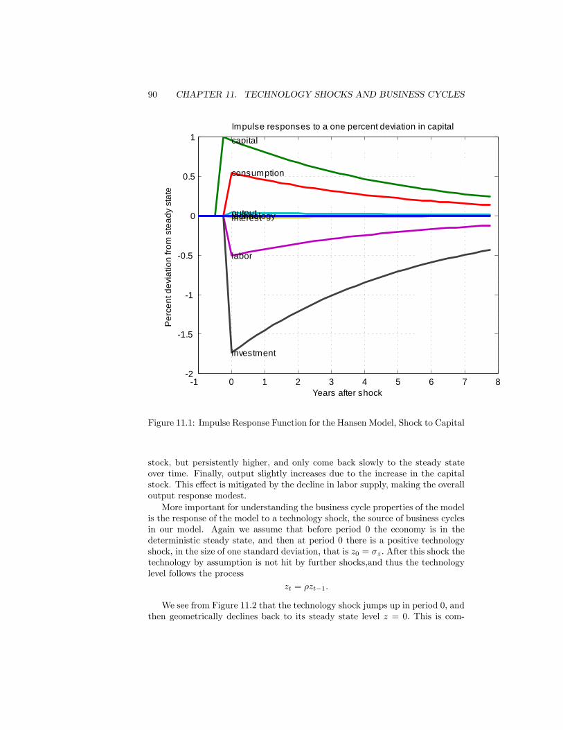
90 CHAPTER 11. TECHNOLOGY SHOCKS AND BUSINESS CYCLES

1 0 1 2 3 4 5 6 7 82

1.5

1

0.5

0

0.5

1Impulse responses to a one percent deviation in capital

Years after shock

Perc

ent d

evia

tion

from

ste

ady

stat

e

capital

consumption

output

labor

interest

investment

technology

Figure 11.1: Impulse Response Function for the Hansen Model, Shock to Capital

stock, but persistently higher, and only come back slowly to the steady stateover time. Finally, output slightly increases due to the increase in the capitalstock. This e¤ect is mitigated by the decline in labor supply, making the overalloutput response modest.More important for understanding the business cycle properties of the model

is the response of the model to a technology shock, the source of business cyclesin our model. Again we assume that before period 0 the economy is in thedeterministic steady state, and then at period 0 there is a positive technologyshock, in the size of one standard deviation, that is z0 = �z: After this shock thetechnology by assumption is not hit by further shocks,and thus the technologylevel follows the process

zt = �zt�1:

We see from Figure 11.2 that the technology shock jumps up in period 0; andthen geometrically declines back to its steady state level z = 0: This is com-

11.1. IMPULSE RESPONSE FUNCTIONS 91

1 0 1 2 3 4 5 6 7 81

0

1

2

3

4

5

6

7

8Impulse responses to a shock in technology

Years after shock

Perc

ent d

evia

tion

from

ste

ady

stat

e

capitalconsumption

outputlabor

interest

investment

technology

Figure 11.2: Implulse Response for the Hansen Model, Technology Shock

pletely by construction, and there is nothing surprising or endogenous aboutthis. The key question is how the endogenous variables of model, capital, con-sumption, consumption etc. respond to the technology shock.The most signi�cant response is in private investment, which on impact

increases by almost 8% on impact. An increase in technology makes capitalmore productive in the future, since future technology is expected to be higher(note that � is close to 1): The social planner responds optimally by immediatelybuilding up the capital stock. Labor supply also responds positively to theincrease in productivity, albeit not as strongly as investment. Consequentlyoutput increases by more than the technology shock: this is the intertemporalsubstitution of labor supply. Consumption also increases, albeit very little, onimpact. The small increase in consumption is due to the fact that it is optimal todevote a lot of the extra production to investment to reap the bene�ts of higherproductivity in the future. Over time investment declines back to the steadystate quite quickly, but consumption remains high for a much longer time, fueled


by the now higher capital stock and the higher productivity. Eventually thetechnology level gets back to the steady state, and so do output, consumption,the capital stock and labor.The key observations from the impulse response analysis for business cycles

is the very strong response of investment on impact of the technology shock,the positive labor supply response, the persistent e¤ect on output due to thepersistence of the technology shock and the increase of the capital stock. Theseproperties of the policy functions will translate into the business cycle propertiesof the model. These properties we will now document by simulating the modeland then comparing the simulated time series from the model to the businesscycle statistics from the data.

11.2 Comparing Business Cycle Statistics of Modeland Data

Once we have the policy functions we can easily simulate the model. Startwith an initial condition for the capital stock, say the steady state level, so thatk0 = 0; and with an initial condition for z; say z0 = 0: Then draw a sequenceof technology shocks1 f"tgTt=0 and construct fztgTt=1 from the equation

zt = �zzt�1 + "t

Once we have the initial condition k0 = 0 and the technology shocks zt; we canuse the policy functions delivered from the software

kt+1 = kzt + skkt

ct = czt + sckt

lt = lzt + slkt

to determine time series fkt+1; ct; ltgTt=1 and thus of course time series forfkt+1; ct; ltgTt=1: Now that we arti�cial data from the model, we can computeexactly the same statistics as we did form the real data. The model is deemedto be a good model of business cycles if the statistics from the model match upfavorably with those from the data.In table 11.1 we summarize the basic business cycle properties of the model,

and, as comparison, of the data, from table 2.1.

We observe that the model is able to generate output volatility of the samemagnitude as found in the data. In addition, the persistence of business cyclesin the model is comparable to that in the data, although the persistence in themodel is somewhat lower than that in the data. Figure 11.3 shows a simulation

1Drawing a seqeunce of independent, normally distributed random variables is a fairlystandard problem for which reliable software exists. The resulting numbers are however, onlypseudo-random numbers, that is, they are generated according to a deterministic function, butlook like random numbers. If you are interested in the mathematical details, I have furtherreferences for you.

11.2. COMPARING BUSINESS CYCLE STATISTICS OFMODEL ANDDATA93

Variable Mean St. Dv. A(1) A(2) A(3) A(4) A(5)Data 0% 1:7% 0; 84 0; 60 0; 32 0; 08 �0; 10Model 0% 2:1% 0; 72 0; 42 0; 16 �0; 05 �0; 21

Table 11.1: Business Cycles: Data and Model

0 5 10 15 20 25 30 35 4020

15

10

5

0

5

10

15

capitalconsumption

outputlabor

interest

investment

technology

Simulated data (HPfiltered)

Year

Per

cent

dev

iatio

n fro

m s

tead

y st

ate

Figure 11.3: Simulated Data from the Hansen Model

of the model for 40 periods, whose summary statistics (for a simulation of longerlength) are displayed in table 11.1. The most outstanding fact from the simu-lation is the high volatility of investment. This is not a surprise, but shows upalready in the impulse response function 11.2. In addition, the high volatility ofinvestment is a salient fact of business cycles in the data: investment demandis by far the most volatile component of GDP.


11.3 Counterfactual Experiments

Set �z = 0Make �z smallerChange utility function for leisure

Part IV

Welfare and PolicyQuestions

95

97

[Next version of these notes]

Chapter 12

The Cost of Business Cycles

99

100 CHAPTER 12. THE COST OF BUSINESS CYCLES

Bibliography

[1] Cooley, T. and E. Prescott (1995), �Economic Growth and Business Cy-cles,� in T. Cooley (ed.), Frontiers of Business Cycle Research, PrincetonUniversity Press, Princeton, N.J.

[2] Hansen and Prescott, Cooley

[3] Kydland and Prescott, Econometrica

[4] Rogerson, R, Journal of Monetary Economics

101

quantitative macroeconomics: an introduction (2).pdf · quantitative macroeconomics: an...

Documents