quantitative imaging biomarkers: a review of statistical methods for

http://smm.sagepub.com/Statistical Methods in Medical Research

http://smm.sagepub.com/content/early/2014/05/30/0962280214537390The online version of this article can be found at:

DOI: 10.1177/0962280214537390

published online 11 June 2014Stat Methods Med ResComparison Working Group)

Daniel P Barboriak, Robert J Gillies, Lawrence H Schwartz, and Daniel C Sullivan and (for the Algorithm Jayashree Kalpathy-Cramer, Tatiyana V Apanasovich, Paul E Kinahan, Kyle J Myers, Dmitry B Goldgof,

(Grace) Kim, Huiman X Barnhart, Edward F Jackson, Maryellen L Giger, Gene Pennello, Alicia Y Toledano, Nancy A Obuchowski, Anthony P Reeves, Erich P Huang, Xiao-Feng Wang, Andrew J Buckler, Hyun J

comparisonsQuantitative imaging biomarkers: A review of statistical methods for computer algorithm

Published by:

http://www.sagepublications.com

can be found at:Statistical Methods in Medical ResearchAdditional services and information for

http://smm.sagepub.com/cgi/alertsEmail Alerts:

http://smm.sagepub.com/subscriptionsSubscriptions:

http://www.sagepub.com/journalsReprints.navReprints:

http://www.sagepub.com/journalsPermissions.navPermissions:

What is This?

- Jun 11, 2014OnlineFirst Version of Record >>

at DUKE UNIV on June 18, 2014smm.sagepub.comDownloaded from at DUKE UNIV on June 18, 2014smm.sagepub.comDownloaded from

http://smm.sagepub.com/

http://smm.sagepub.com/content/early/2014/05/30/0962280214537390

http://www.sagepublications.com

http://smm.sagepub.com/cgi/alerts

http://smm.sagepub.com/subscriptions

http://www.sagepub.com/journalsReprints.nav

http://www.sagepub.com/journalsPermissions.nav

http://smm.sagepub.com/content/early/2014/05/30/0962280214537390.full.pdf

http://online.sagepub.com/site/sphelp/vorhelp.xhtml



XML Template (2014) [27.5.2014–2:59pm] [1–39]//blrnas3/cenpro/ApplicationFiles/Journals/SAGE/3B2/SMMJ/Vol00000/140065/APPFile/SG-SMMJ140065.3d (SMM) [PREPRINTER stage]

Article

Quantitative imagingbiomarkers: A review ofstatistical methods for computeralgorithm comparisons

Nancy A Obuchowski,1 Anthony P Reeves,2

Erich P Huang,3

Xiao-Feng Wang,1 Andrew J Buckler,4 Hyun J (Grace) Kim,5

Huiman X Barnhart,6 Edward F Jackson,7 Maryellen L Giger,8

Gene Pennello,9 Alicia Y Toledano,10

Jayashree Kalpathy-Cramer,11 Tatiyana V Apanasovich,12

Paul E Kinahan,13 Kyle J Myers,9 Dmitry B Goldgof,14

Daniel P Barboriak,6 Robert J Gillies,15 Lawrence H Schwartz,16

and Daniel C Sullivan6 (for the Algorithm Comparison WorkingGroup)

Abstract

Quantitative biomarkers from medical images are becoming important tools for clinical diagnosis, staging,

monitoring, treatment planning, and development of new therapies. While there is a rich history of the

development of quantitative imaging biomarker (QIB) techniques, little attention has been paid to the

validation and comparison of the computer algorithms that implement the QIB measurements. In this

1Cleveland Clinic Foundation, Cleveland, OH, USA2Cornell University, Ithaca, NY, USA3National Institutes of Health, Rockville, MD, USA4Elucid Bioimaging Inc., Wenham, MA, USA5University of California, Los Angeles, CA, USA6Duke University, Durham, NC, USA7University of Wisconsin-Madison, Madison, WI, USA8University of Chicago, Chicago, IL, USA9Food and Drug Administration/CDRH, Silver Spring, MD, USA10Biostatistics Consulting, LLC, Kensington, MD, USA11MGH/Harvard Medical School, Boston, MA, USA12George Washington University, NW Washington, DC, USA13University of Washington, Seattle, WA, USA14University of South Florida, Tampa, FL, USA15H. Moffitt Cancer Center, Tampa, FL, USA16Columbia University, New York, NY, USA

Corresponding author:

Nancy A Obuchowski, Quantitative Health Sciences/JJN 3, Cleveland Clinic Foundation, 9500 Euclid Ave, Cleveland,

OH 44195, USA.

Email: [email protected]

Statistical Methods in Medical Research

0(0) 1–39

! The Author(s) 2014

Reprints and permissions:

sagepub.co.uk/journalsPermissions.nav

DOI: 10.1177/0962280214537390

smm.sagepub.com

at DUKE UNIV on June 18, 2014smm.sagepub.comDownloaded from



paper we provide a framework for QIB algorithm comparisons. We first review and compare various

study designs, including designs with the true value (e.g. phantoms, digital reference images, and zero-

change studies), designs with a reference standard (e.g. studies testing equivalence with a reference

standard), and designs without a reference standard (e.g. agreement studies and studies of algorithm

precision). The statistical methods for comparing QIB algorithms are then presented for various study

types using both aggregate and disaggregate approaches. We propose a series of steps for establishing the

performance of a QIB algorithm, identify limitations in the current statistical literature, and suggest future

directions for research.

Keywords

quantitative imaging, imaging biomarkers, image metrics, bias, precision, repeatability, reproducibility,

agreement

1 Background and problem statement

Medical imaging is an effective tool for clinical diagnosis, staging, monitoring, treatment planning,and assessing response to therapy. In addition it is a powerful tool in the development of newtherapies. Measurements of anatomical, physiological, and biochemical characteristics of thebody through medical imaging, referred to as quantitative imaging biomarkers (QIBs), arebecoming increasingly used in clinical research for drug and medical device development andclinical decision-making.

A biomarker is defined generically as an objectively measured indicator of a normal orpathological process or pharmacologic response to treatment.1,2 In this paper, we focus on QIBs,defined as imaging biomarkers which consist of a measurand only (variable of interest) ormeasurand and other factors (e.g. body weight) that may be held constant and the differencebetween two values of the QIB is meaningful. In many cases there is a clear definition of zerosuch that the ratio of two values of the QIB is meaningful.3,4

Most QIBs requires a computation algorithm, which may be simple or highly complex. Anexample of a simple computation is measurement of a nodule diameter on a 2D x-ray image.A slightly more complex example is the estimation of the value of the voxel with the higheststandardized uptake value (SUV, a measure of relative tracer uptake) within a pre-defined regionof interest in a volumetric positron emission tomography (PET) image. Even more complex methodsexist, such as the estimation of Ktrans, the volume transfer constant between the vascular space andthe extravascular, extracellular space from a dynamic contrast-agent-enhanced magnetic resonanceimaging (MRI) sequence, where an a priori physiological model is used to fit the measured time-dependent contrast enhancement measurements. In this paper, we consider QIBs generated fromcomputer algorithms, whether or not the computer algorithm requires human involvement.

While there is a rich history of the development of QIB techniques, there has been comparativelylittle attention paid to the evaluation and comparison of the algorithms used to produce the QIBresults. Estimation errors in algorithm output can arise from several sources during both imageformation and the algorithmic estimation of the QIB (see Figure 1). These errors combine(additively or non-additively) with the inherent underlying biological variation of the biomarker.Studies are thus needed to evaluate the imaging biomarker assay with respect to bias, defined as theexpected difference between the biomarker measurement (measurand) and the true value,3 and

2 Statistical Methods in Medical Research 0(0)




precision, defined as the closeness of agreement between values of the biomarker measurement onthe same experimental unit.3

There are several challenges in the evaluation and adoption of QIB algorithms. A recurring issueis the lack of reported estimation errors associated with the output of the QIB. One example is theroutine reporting in clinical reports of PET SUVs with no confidence intervals (CIs) to quantifymeasurement uncertainty. If the measure of a patient’s disease progression versus response totherapy is determined based on changes of SUV �30%, for example, then the need to state theSUV measurement uncertainties for each scan becomes apparent.

Another challenge is the inappropriate choice of biomarker metrics and/or parametric statistics.For example, tumor volume doubling time is sometimes used in studies as a QIB. However, it maynot be appropriate to use the mean as the parametric statistic for an inverted, non-normal,measurement space. Since a zero growth rate corresponds to a doubling time of infinity, it is easyto see that parametric statistics based on tumor volume doubling time (e.g. mean doubling time)may be skewed and/or not properly representative of the population. See Yankelevitz5 and Lindellet al.6 for further discussion.

CIs, or some variant thereof, are needed for a valid metrology standard. However, many studiesinappropriately use tests of significance, e.g. p values, in place of appropriate metrics. In addition,there may be discordance between what might be a superior metric statistically and what is clinicallyacceptable or considered clinically relevant. For example, a more precise measuring method willtypically better predict the medical condition, but only until the measurement precision exceedsnormal biological variation; further improvement in precision will offer no significant improvementin efficacy. Finally, when potentially improved algorithms are developed, data from previous studiesare often not in a form that allows new algorithms to be tested against the original data. Publiclyavailable databases of clinical images are being developed to provide a resource of images withappropriate documentation that may be used for computer algorithm evaluation and comparison.Three notable examples are (1) the Lung Imaging Database Consortium (LIDC), which makesavailable a database of computed tomography (CT) images of lung lesions that have beenevaluated by experienced radiologists for comparison of lesion detection and segmentationalgorithms,7 (2) the Reference Image Database for Evaluation of Response (RIDER), whichcontains sets of CT, PET, and PET/CT patient images before and after therapy, as well as test/retest, assumed zero-change, MR data sets from phantoms, human brain and breast8 (https://wiki.nci.nih.gov/display/CIP/RIDER), and (3) the Retrospective Image Registration EvaluationProject (www.insight-journal.org/rire/), which allows open source data retrospective comparisonsof CT-MRI and PET-MRI image registration techniques Other such databases can be found athttp://www.via.cornell.edu/databases/

Figure 1. The role of quantitative medical imaging algorithms and dependency of the estimated QIB on sources

of bias and precision.

Obuchowski et al. 3




This paper is motivated by the activities of the Radiological Society of North America (RSNA)Quantitative Imaging Biomarkers Alliance (QIBA).9 The mission of QIBA is to improve the valueand practicality of QIBs by reducing variability across devices, patients, and time. A cornerstone ofthe QIBA methodology is to produce a description of a QIB in sufficient detail that it can beconsidered a validated assay,4 which means that the measurement bias and variability are bothcharacterized and minimized. This is accomplished through the use of a QIBA ‘Profile’, which isa document intended for a broad audience including scanner and third-party device manufacturers(e.g. display stations), pharmaceutical companies, diagnostic agent manufacturers, medical imagingsites, imaging contract research organizations, physicians, technologists, researchers, professionalorganizations, and accreditation and regulatory authorities. A QIBA Profile has the followingcomponents:

(1) A description of the intended use of, or clinical context for, the QIB.(2) A ‘claim’ of the achievable minimum variability and/or bias.(3) A description of the image acquisition protocol needed to meet the QIBA claim.(4) A description of compliance items needed to meet the QIBA claim.

In a QIBA Profile, the claim is the central result, and describes the QIB as a standardized,reproducible assay in terms of technical performance. The QIBA claim is based on peer-reviewedresults as much as possible, and also represents a consensus opinion by recognized experts in theimaging modality. For example, the QIBA fluorodeoxyglucose (FDG)-PET/CT Profile10 was basedon nine original research studies,11–19 one meta-analysis,20 and two multi-center studies that are inthe process of being submitted for publication, as well as review by over 100 experts. During theinitial development of the profiles from the various QIBA Technical Committees, it was realized thatdifferent metrics were being used to describe the minimum achievable variability and/or bias, andthat quantitative comparisons of the corresponding QIBs required a careful description of the goalsof the comparison, the available data, and the means of comparison. This comparison is animportant precursor to the final goal (Figure 1) of providing information as a tool for clinicalimaging or in clinical trials.

The specific goals of this paper are to provide a framework for QIB algorithm comparisons by areview and critique of study design (Section 2), general statistical hypothesis testing and CI methodsas they commonly apply to QIBs (Section 3), followed by several sections on statistical methods foralgorithm comparison. First we address approaches to estimating and comparing algorithms’ biaswhen the true value or a reference standard is present (Section 4); then we address the more difficulttask of estimating and comparing bias when there is no true value or suitable reference standardavailable (Section 5). In Section 6 we review the statistical methods for assessing agreement andreliability among QIB algorithms. We discuss methods for estimating and comparing algorithms’precision in Section 7. Finally, we link the preceding sections to a process for establishing theeffectiveness of QIBs for implementation or marketing with defined technical performance claims(Section 8). There is a discussion of future directions in Section 9.

2 Study design issues for QIB algorithm comparisons

There are two common types of studies for comparing QIB algorithms: (a) studies to characterizethe bias and precision in the measuring device/imaging algorithm/assay and (b) studies to determinethe clinical efficacy of the biomarker. It is the former that is the main focus of this paper. Clinicalefficacy requires a distinct set of study questions, designs, and statistical approaches to address and is





beyond the scope of this paper. Once a QIB has been optimized to minimize measurement bias andprecision, then traditional clinical studies to evaluate clinical efficacy may be conducted. Efficacy forclinical practice can be evaluated from clinical studies that correlate clinical outcomes to one ormore measurements for the biomarker.

There are several different QIB types (Table 1). When designing a study it is important to evaluateand report the correct measurement type. For example, in measuring lesion size there are at leastthree different measurement types: absolute size assessed from a single image, a change in sizeassessed from a sequential pair of images, and growth rate assessed from two or more imagesrecorded at known time intervals. Each of these has a different measurand and associateduncertainty; characterizing one type does not mean that other types are characterized. A relatedissue is the suitability of a measurand for statistical analysis. For example, if in a set of change-in-size measurements one case has a measured value of no change (i.e. zero) then the doubling time forthat case is infinity. Further estimating the mean doubling time for a set of cases that include thiscase will also have a value of infinity. If the reciprocal scale of growth rate is used for a study thenthese problems do not occur. The results of the study can be translated back to the doubling timesfor presentation in the discussion.

There is a number of common research questions asked in QIB algorithm comparison studies.They range from which algorithms have lower bias and more precision to more complex questionssuch as which algorithms are equivalent to a reference standard. Different study designs are neededto answer these questions. Table 2 lists several common questions addressed in QIB comparisonstudies and the corresponding design requirements needed.

Studies on QIBs face two challenges that may not plague the evaluation of quantitative in vitrobiomarkers: the need for human involvement in extracting the measurement and the lack of the truevalue. For many QIBs, human involvement in making the actual measurement is often permitted orrequired. In some cases fully automated measurement is possible; therefore, both approaches need tobe considered in designing studies. In patient studies of QIBs, the true value of the biomarker isoften not available. Histology or pathology tests are often used as the true value, but these are moreappropriately referred to as reference standards, defined as well-accepted or commonly usedmethods for measuring the biomarker but have associated bias and/or measurement error. Forexample, histology and pathology are known to have sampling errors due to tissue heterogeneityand the non-quantitative nature of histopathology tests, as well as requiring human subjectiveinterpretation. One situation where some data are available is the use of test–retest designs wherepatients are imaged over a short period of time (often less than an hour) when no therapy is beingadministered so that no appreciable biologic change can occur. We discuss both of these issues infurther detail.

Human intervention with a QIB algorithm is a major consideration for the study design. With anautomated algorithm all that is required is the true value for the desired outcome and standardmachine learning methodology may be employed. The algorithm may then be exhaustively evaluatedwith very large documented data sets with many repetitions as long as a valid train/test methodologyis employed. When human intervention is part of the algorithm, then observer study methodologymust be employed. First, the image workstation must meet accepted standards for effective humanimage review. Second, the users/observers must be trained and tested for the correct use of thealgorithm. Third, careful consideration must be given to the workflow and conditions under whichthe human ‘‘subjects’’ perform their tasks in order to minimize the effects of human fatigue. Finally,there is a need to characterize the between- and within-reader effects due to operator variability. Themost serious limitation of the human intervention studies is the high cost of measuring each case;this limits the number of data examples that can be evaluated. Typically the number of cases used for

Obuchowski et al. 5




Table 1. Types of QIB measurements with examples.

Measurement type Parameters Measurand Examples and explanations

Extent Single image V, L, A, D, I, SUV Volume (V), length (L), area (A), diameter in 2D

image (D), intensity (I) of an image or region of

interest (ROI), SUV (a measure of relative tracer

uptake).

Geometric form Single or multiple

images

VX, AX Set of locations of all the pixels or voxels that

comprise an object in an image or ROI; the

overlap of two images.

Geometric location Single or multiple

images

Distance Distance relative to the true value or reference

standard or between two measurements;

distance between two centers of mass; location

of a peak.

Proportional change Two or more repeat

images

2ðV2�V1Þ

ðV1þV2ÞFractional change in A or V or L or D or I measured

from ROIs of two or more images. Response-to-

therapy may be indicated by a lesion increasing in

size (progression of disease¼ PD), not changing

in size (stable disease¼ SD), or decreasing in size

(response to therapy¼RT). The magnitude of

the change may also be important (e.g. cardiac

ejection fraction).

Growth rate Two or more repeat

images and time

intervals

½ðV2=V1Þ1=�t � 1� Proportional change per unit time in A or V or D or I

of an ROI from two or more images with respect

to an interval of time �t. Malignant lesions are

considered to have a high approximately

constant growth rate (i.e. have volumes that

increase exponentially in time). Benign nodules

are usually slow growing.

Morphological and

texture features

Single or multiple

images

CIR, IR, MS,

AF, SGLDM,

FD, FT, EM

Boundary aspects including surface curvature such

as circularity (CIR), irregularity (IR), and

boundary gradients such as margin sharpness

(MS). Texture features of an ROI: grey level

statistics, autocorrelation function (AF), Spatial

Gray Level Dependence Measures (SGLDM),

Fractal dimension measures (FD), Fourier

transform measures (FT), energy measures (EM).

Kinetic response Two or more repeat

images during the

same session

f(t), Ktrans, ROI(t) The values of pixels change due to the response to

an external stimulus, such as the uptake of an

intravenous contrast agent (e.g. yielding Ktrans) or

an uptake of a radioisotope tracer (ROI(t)). The

change in these values is related to a kinetic

model.

Multiple acquisition

protocols

Two or more repeat

images with

different protocols

during same

session

ADC, BMD, fractional

anisotropy

ADC: apparent diffusion coefficient, BMD: bone

mineral density. Unlike other QIBs considered

here, morphological and texture features may

not be evaluable with some of the statistical

methods described since they do not usually

have a well-defined objective function.





observer studies varies from a few 10’s to a few 100’s at most. This is an important limitation whencharacterizing the performance of an algorithm with respect to an abnormal target such as a lesion.Because disease abnormalities have no well-defined morphology and may offer a wide (maybeinfinite) spectrum of image presentations, large sample sizes are often required to fullycharacterize the performance of the algorithm. In contrast, studies on automated methods areessentially unlimited in the number of cases that could be evaluated and are currently typicallylimited by the number of cases that can be made available.

Ideal data that would fully characterize bias and precision and thus validate algorithmperformance is usually not available. For example, no technique exists to validate that an in vivolesion size volume measurement is correct. If we were able to determine lesion size using pathologicalinspection, then we still could not validate a lesion size growth rate measurement since we wouldneed to have a high precision volume measurement at two time points. This is in contrast to otherquantitative biomarkers such as the fever thermometer, which may easily be compared to a superior-quality higher-precision verified reference thermometer. With no direct method for measurementevaluation a number of indirect methods have been developed. The three main indirect approachesare: phantoms (physical test objects) or digital (synthetic) reference images, experienced physicianmarkings, and zero-change data sets. Note, though, that none of these designs can achieve the fullcharacterization of the measurement uncertainty that is desired.

Phantoms are physical models of the target of interest and are imaged using the same machinesettings. Digital reference images are synthetic images that have been created by computersimulations of a target in its environment; the image acquisition device (i.e. scanner) is notinvolved but similar noise artifacts are added to the image. An advantage of these approaches is

Table 2. Common research questions and corresponding design requirements.

Research question: Study design requirements

1. Which algorithm(s) provides measurements such

that the mean of the measurements for an

individual subject is closest to the true value for

that subject (comparison of individual bias)?

The true value, and replicate measurements by each

algorithm for each subject

2. Which algorithm(s) provides the most precise

measurements under identical testing conditions

(comparison of repeatability)?

Replicate measurements by each algorithm for each

subject

3. Which algorithm(s) provides the most precise

measurements under testing conditions that vary

in location, operator, or measurement systema

(comparison of reproducibility)?

One or more replicate measurements for each

testing condition by each algorithm for each

subject

4. Which algorithm provides the closest

measurement to the truth (comparison of

aggregate performance)?

The true value, and one or more replicate

measurements by each algorithm for each subject

5. Which algorithm(s) are interchangeable with a

Reference Standard (assessment of individual

agreement)?

Replicate measurements by the reference standard

for each subject, and one or more replicate

measurements by each algorithm for each subject

6. Which algorithm(s) agree with each other

(assessment of agreement or reliability)?

One or more replicate measurements by each

algorithm for each subject

aMeasurement system refers to how the data were collected prior to analysis by the algorithm(s), e.g. what type of scanning

hardware was used, what settings were applied during the acquisition, what protocol was used by the operator, etc.

Obuchowski et al. 7




that the true value is known. A disadvantage of the synthetic image approach is that currently thesemethods are approximations to the real images and do not faithfully represent all the importantsubtleties encountered in real images, especially the second or higher order moments of the data(e.g. the correlation structure in the image background). Phantoms and digital reference images maybe used to establish a minimum performance requirement for QIB algorithms. That is, anyalgorithm should not make ‘‘large’’ errors on such a simplified data set. However, one danger isthat an algorithm may be optimized for high performance on just the simplified phantom modeldata; such an algorithm may not work at all on real data. Therefore, superior performance of analgorithm on phantom data does not imply superior performance on real in vivo data. For example,phantom pulmonary nodules have several properties that differ from real pulmonary nodulesincluding smooth surfaces, sharp margins, known geometric elemental shapes (spheroids andconics), homogeneous density, no vascular interactions, no micro-vascular artifacts, and nopatient-motion artifacts. An algorithm that is optimized to any of these properties may appear tohave overly optimistic performance when applied to real in vivo data.

The main issue with having experienced physicians set the reference standard by, for example,marking the boundary of a target lesion of interest in the image in order to determine the targetvolume, is that studies have shown that such markings have a very large degree of inter-readervariation.21 Therefore, it is not possible, in general, to use physicians’ marking as the true value.Researchers are working to develop computer algorithms that have less uncertainty than evenexperienced physician judgments.

Zero-change and test/retest studies take advantage of situations where two or moremeasurements may be made of a target lesion when it is known or assumed that there isinsufficient time between measurements for there to be any biological change in the lesion. Oneversion of this is referred to as a ‘‘coffee break’’ study where the subject is scanned, then removedfrom the scanner for a few minutes (‘‘coffee break’’), and then repositioned and scanned again.Hence the true value (e.g. tumor volume) is assumed to be the same for the two measurementsalthough the actual true value is unknown. Frequently, such studies take advantage of opportunisticimage protocols and are limited to a single repeated measure due to possible harms to the patientfrom reimaging. These studies are important when true values are not available since they providesome information of the truth for a special case (i.e. zero-change). When viewed as measurementsfrom a single time point, these studies provide repeated measures to better estimate the precision ofthe measurement method across a range of volumes. When considered in a scenario of two timepoints (where the focus is on measuring change), the coffee break study provides an aggregateestimate of bias and precision at the single measurement point of no change.

While test–retest studies have several advantages over phantom studies, they are often difficult tooperationalize in practice. An example of one that is relatively straightforward is CT measurementsof lung lesions where no contrast agent is used. As noted above, the patient is scanned, leaves thescan table for a short period of time, and then is re-scanned. A more challenging example is the samemeasurement, but in the liver. This is more challenging because contrast agent is often used. If thesame ‘‘coffee break’’ methodology was used, the second scan might have relatively large changes inthe phase of the contrast in the liver so differences in measurement would be convolved with thedesired ‘‘no change’’ condition. To compensate for this, one would have to perform the test–reteststudy using a second injection of contrast following sufficient wash-out time of the first, and thencapture the same phase as in the first measurement. However, such a protocol is unlikely to beacceptable to an Institutional Review Board (IRB), let alone the patients themselves.

A further limitation of the test–retest approach is that it does not address (include) severalsources of measurement error associated with time intervals relevant to clinical practice; these





include: variation in patient state, variation in machine calibration, and possible change in imagingdevice (model or software) between images. Finally, the zero-change method includes the errors ofboth the imaging system and the measurement algorithm. If the error introduced by the imagingsystem is of a similar magnitude to the precision of the algorithm then care must be taken whencomparing multiple algorithms to include the image system error in the comparative analysis.22

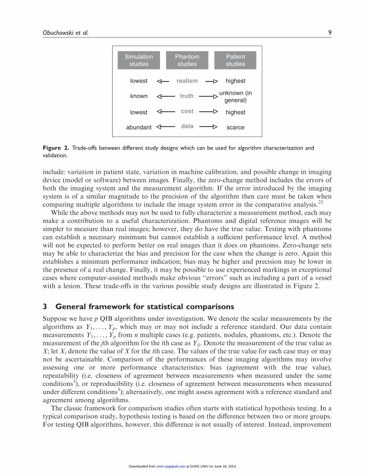
While the above methods may not be used to fully characterize a measurement method, each maymake a contribution to a useful characterization. Phantoms and digital reference images will besimpler to measure than real images; however, they do have the true value. Testing with phantomscan establish a necessary minimum but cannot establish a sufficient performance level. A methodwill not be expected to perform better on real images than it does on phantoms. Zero-change setsmay be able to characterize the bias and precision for the case when the change is zero. Again thisestablishes a minimum performance indication; bias may be higher and precision may be lower inthe presence of a real change. Finally, it may be possible to use experienced markings in exceptionalcases where computer-assisted methods make obvious ‘‘errors’’ such as including a part of a vesselwith a lesion. These trade-offs in the various possible study designs are illustrated in Figure 2.

3 General framework for statistical comparisons

Suppose we have p QIB algorithms under investigation. We denote the scalar measurements by thealgorithms as Y1, . . . ,Yp, which may or may not include a reference standard. Our data containmeasurements Y1, . . . ,Yp from n multiple cases (e.g. patients, nodules, phantoms, etc.). Denote themeasurement of the jth algorithm for the ith case as Yij. Denote the measurement of the true value asX; let Xi denote the value of X for the ith case. The values of the true value for each case may or maynot be ascertainable. Comparison of the performances of these imaging algorithms may involveassessing one or more performance characteristics: bias (agreement with the true value),repeatability (i.e. closeness of agreement between measurements when measured under the sameconditions3), or reproducibility (i.e. closeness of agreement between measurements when measuredunder different conditions3); alternatively, one might assess agreement with a reference standard andagreement among algorithms.

The classic framework for comparison studies often starts with statistical hypothesis testing. In atypical comparison study, hypothesis testing is based on the difference between two or more groups.For testing QIB algorithms, however, this difference is not usually of interest. Instead, improvement

Simulationstudies

Phantomstudies

Patientstudies

highestlowest

unknown (ingeneral)

known

highestlowest

realism

truth

cost

scarceabundant data

Figure 2. Trade-offs between different study designs which can be used for algorithm characterization and

validation.

Obuchowski et al. 9




or equivalence or non-inferiority (NI) is often the interest when comparing QIB algorithms. Forexample, in a phantom or zero-change study, one may want to test improvement or equivalence inabsolute value of bias of the new method versus old method. The former leads to a superiority testand the latter to an equivalence test. In a clinical validity or agreement study, one may be interestedin testing whether two or more algorithms’ repeatability or reproducibility is non-inferior with aclinically meaningful threshold. The statistical hypotheses and corresponding statistical tests aregiven below for each of these situations. We also provide the analogous CI approach, which isoften preferable to statistical hypothesis testing because it provides critical information about themagnitude of the bias and precision of QIB algorithms.

3.1 Testing superiority

A typical scenario in QIB studies is to show improvement of a new or upgraded algorithm over astandard algorithm. The one-sided testing for superiority for a QIB algorithm is described by thenull and alternative hypotheses:

H0 : � � �o vs : HA : �5 �o ð1Þ

where � is the parameter for the difference in performance characteristics (e.g. measures of biasor repeatability) between two algorithms and is estimated by T�S, where T is the estimatedvalue from the proposed algorithm (i.e. estimated from Yij’s) and S is the estimated value from astandard/control or competing algorithm. �o is the pre-defined allowable difference (sometimesset to zero). Typically in QIB algorithm comparison studies, smaller values of T relative to Sindicate that the investigational algorithm is preferred (i.e. less bias, or less uncertainty). Forexample, T might be the estimated absolute value of the percent error of a proposed algorithmand S is the estimated value from a standard algorithm. The test statistic is: t¼ (T�S)/SE(T�S),where SE(T�S) is the sample standard error of T�S calculated assuming the null hypothesis,�¼ 0, is true. We reject H0 and conclude superiority of the proposed algorithm to the standard,if t< t�,� (a one-sided �-level test, � degrees of freedom). Note that testing is not limited to thecase of mean statistics (e.g. mean of the Yij’s) but rather can be applied for metrics ofperformance such as repeatability and reproducibility. If larger values of T, e.g. reliability,relative to S indicate the proposed algorithm is preferred, then the null and alternativehypotheses should be reversed. When the normal assumption is invalid, two choices can beconsidered: (a) transformation of a measurement based on the Box-Cox regression, (b)nonparametric and bootstrap methods.23

In many cases a preferable approach is to use the CI approach. To declare superiority, we need toshow that the one-sided 100� (1� �)% CI, (�1, Cu) for T�S, is included in (�1, 0), or Cu< 0, asshown in the following sketch, where Cu is the upper limit of the CI.





3.2 Testing equivalence

In order to perform an equivalence test, appropriate lower and/or upper equivalence limits on � needto be defined by the researcher prior to the study. The limits are sometimes based on an arbitrarylevel of similarity such as allowing for a 10% difference, or based on prior knowledge of imagingmodalities and algorithms. Schuirmann24 proposed the two one-sided testing (TOST) procedure,which has been widely used for testing bioequivalence in clinical pharmacology. The TOSTprocedure consists of the null and alternative hypotheses:

H0 : � � �L or � � �U vs: HA : �L 5 �5 �U ð2Þ

�L and �U are the lower and upper equivalence limits of �. The limits of � (i.e. �) should be pre-specified based on scientific or clinical judgment. Practically speaking, � should be a meaningfuldifference to the developer of the algorithm or clinically meaningful in algorithm comparison,beyond an arbitrary positive value. It may be sufficient to assume that data from two algorithmsare normally distributed with the same unknown variance, and the equivalence interval issymmetrical about zero, i.e. �¼��L, �U. Thus, the critical region of TOST at the level � is

CR ¼ ðT� S�

Þ � �g= sp 1=n1 þ 1=n2ð Þ1=2

� �� t1��, �

and

ðT� S�

Þ � �g= sp 1=n1 þ 1=n2ð Þ1=2

� �� t�,�

where n1 and n2 are the study sample sizes of a proposed algorithm and standard, respectively, s2p isthe pooled sample variance, and t1� �,� and t�,� are the 100(1� �)% and 100�% percentiles of a tdistribution with �¼ n1þ n2� 2 degrees of freedom.25 If T and S are sample means, then the pooledsample variance is ffiffiffiffiffiffiffiffiffiffiffiffiffiffiffiffiffiffiffiffiffiffiffiffiffiffiffiffiffiffiffiffiffiffiffiffiffiffiffiffiffiffiffiffiffiffiffiffiffiffiffiffiffiffiffiffiffiffiffiffiffiffiffiffiPn1

i¼1ðYi � TÞ2 þPn2

i¼1ðXi � SÞ2

ðn1 þ n2 � 2Þ

s

In the CI approach, we need to show that 100� (1� 2�)% CI, [CL, CU], is included in [��, �], orthat ��<Cu<CL<�, where CL and CU are the lower and upper limits of the CI, respectively.

3.3 Testing NI

When a researcher wants to demonstrate that a QIB algorithm is no less biased or no less reliable orno less reproducible than a standard method or another competing algorithm, testing for NI isappropriate. NI does not simply mean not inferior but rather not inferior by as much as a

Obuchowski et al. 11




predetermined margin, with respect to a particular measurement under study. This may involve anassessment of NI and superiority in a stepwise fashion. Because there is incentive to demonstratesuperior performance beyond NI, the interest is fundamentally one-sided. The procedure consists ofthe null and alternative hypotheses,

H0 : � � �1 vs: HA : �5 �1 ð3Þ

where �1 is a pre-defined NI margin for �. �� 1 represents the proposed algorithm is inferior to thestandard by �1 or more, and � <�1 represents the proposed algorithm is inferior to the standard byless than �1. Again, typically in a QIB study, smaller values of T indicate better performance. Thetest statistic is t¼ [(T�S)� �1]/SE(T�S). We reject H0 and conclude NI of the proposed algorithmto the standard if t> t�,v (a one-sided �-level test, v degrees of freedom). Similarly, to declare NI ofthe proposed algorithm to the standard using the CI approach, we need to show that the one-sided100� (1� �)% CI, (�1, Cu) for T�S is included (�1, �1) as shown below. As the second step, ifNI is demonstrated, superiority can be assessed using a two-sided hypothesis test or CI. To preservethe overall significance level of the study, �, we do not perform such an assessment if NI is notdemonstrated.

Examples of NI are illustrated below:

(1) Point estimate of T�S is 0; NI is demonstrated.(2) Point estimate of T�S favors S; NI is not demonstrated.(3) Point estimate of T�S is 0; NI is not demonstrated.(4) Point estimate of T�S favors T; NI is demonstrated, but superiority is not demonstrated.(5) Point estimate of T�S favors T; NI is demonstrated, and superiority is also demonstrated.(6) Point estimate of T�S favors S; NI is demonstrated. S is statistically superior to T.





In examples 1, 4, 5, and 6, NI is demonstrated and under the stepwise scenario superiority can beassessed without adjusting for multiple comparisons.

The methodology for comparing the performance of QIB algorithms depends on the studydesign, the research question, the availability of the true value of the measurement, and theperformance metric. Figure 3 illustrates the decision-making process for determining theappropriate statistical methodology. Details of the methods are given in Sections 4–7.

4 Evaluating performance when the true value or referencestandard is present

The type of QIB algorithm comparison study can be classified based on whether the true value of ameasurement is available or not.26 Sometimes a reference standard can be treated as the true value if

Is it reasonable to assume a linear relationship between

the true value and the algorithms’ measurements?

Compare algorithms based on precision (Section 7)

No Yes

Assess agreement between algorithms (Section 6)

Do you want to assess the interchangeability of algorithms?

Yes

No

Compare algorithms using Regression without Truth

(Section 5)

Yes

Are there replicate measurements foreach algorithm?

Yes

No

Yes

Do you need to compare algorithms relative to truth?

Is the true value of the measurement available?

Assess bias and precision separately or aggregated. Assess individual agreement to a reference standard*. (Section 4)

Is there a reference standard* available that can be treated as the true value or that you want to test individual equivalence against?

Yes

No

Figure 3. Decision tree for identifying statistical methods for a QIB algorithm comparison study. *Reference

standard, defined as a well-accepted or commonly used method for measuring the biomarker but with recognized bias

and/or measurement error. Examples of reference standards are histology, expert human readers, or a state-of-the-

art QIB algorithm.





it has negligible error, as defined by the clinical need of the QIB.4 Comparison problems inquantitative imaging studies where the true value is present are common. Ardekani et al.27

described a study of motion detection in functional MRI (fMRI) where three motion detectionprograms were compared to simulated fMRI data. Prigent et al.28 induced myocardial infarcts indogs and measured infarct size by two methods versus pathologic examination (reference standardtreated as the true value).

There are two general approaches to evaluate the degree of closeness between measurements byan algorithm and the true value: disaggregated and aggregated approaches. In the disaggregatedapproach, the performance of the algorithm is characterized by two components: bias and precision.We would assert that the algorithm performs well if the algorithm has both small bias and highprecision. In the aggregated approach, the performance of the algorithm is evaluated by a type ofagreement index which aggregates information on bias and precision. With this approach we wouldassert that the algorithm is performing well if there is ‘‘sufficient’’ degree of closeness judged by theagreement index between the algorithm and the true value. If substantial disagreement is found, thenthe sources of disagreement, i.e. bias or precision or both, can be investigated. It is possible that analgorithm may be claimed to perform well in one approach, but not the other; therefore, it isimportant to specify which approach is to be used a priori.

In this section we consider both disaggregate (subsection 4.1) and aggregate (subsection 4.2)approaches to evaluating the degree to which the algorithms agree with the true value. We alsodiscuss methods for comparing algorithms against a reference standard to determine if the algorithmcan replace the reference standard (subsection 4.3).

4.1 Disaggregate approaches to evaluating agreement with truth

We first consider the simple situation of one algorithm compared with the true value withoutreplications. Consider a simple model with equal bias and precision across the n cases

Yi ¼ Xi þ "i ¼ 1, . . . , n ð4Þ

where Yi is the measurement on the ith case using an imaging algorithm, Xi is the corresponding truevalue measurement, and "i is the measurement error that is assumed to be independent of Xi, withmean d and variance �2� .

There are two types of biases: individual bias and population bias. They are equal only if theindividual bias is the same for all cases. Individual bias is defined as the expected difference betweenmeasurements by an algorithm and the true value for a case. It describes a systemic inaccuracy in theindividual due to the characteristics of the imaging process employed in the creation, collection, andcomputer algorithm implementation. An estimate of individual bias for case i is Di, which is themeasurement error of the case, Di ¼ "i ¼ Yi � Xi. The studied cases may have a tendency for thealgorithm to be greater or less than the true value. The population bias is a measure of this tendency,which is defined as the expectation of the difference between the algorithm and the true value in thewhole population. The population bias for the simple model is d, the mean parameter for themeasurement error distribution. It can be estimated by the sample mean difference, �d, the meanof the Di’s. A CI can be constructed for the population bias by using the standard error of thesample mean difference.

Correspondingly, there are also two types of precision: individual precision and populationprecision. They are equal only if the individual precision is the same for all cases. If the precisionunder consideration is repeatability and it is expressed as variance, then the individual precision is





defined as the variability between replications on a case; the population precision is the pooledvariability of individual precision across all cases in the population. In general, if there arereplications on each case, the individual precision for a case can be estimated by the samplevariance of the replications on this case. If there are no replications, then estimation would needto rely on model assumptions. For example, under assumptions of the simple model in equation (4)where there are no replications, the individual precision is ðYi � Xi � d Þ for case i, which can beestimated by n

n�1 ðYi � Xi ��d Þ2. The population precision is represented by �2� , the variance

parameter of the measurement error, which can be estimated as the average of the individualprecisions, 1

n�1

Pni¼1ðYi � Xi �

�d Þ2, which is also the sample variance of the Di’s.If the acceptable levels of bias and precision are d0� 0 and �20 , respectively, then the algorithm

may be claimed to perform well if both jdj � d0 and �2� � �20 (i.e. NI hypotheses as in equation 3).

A CI approach may be used to confirm the claims.The population bias may not be fixed but may be proportional to the true value. This occurs

if there is a linear relationship between the QIB and the true value, i.e. linearity holds, but theslope is not equal to one.4 Linear regression is a commonly used approach which can be appliedfor detecting and quantifying not only fixed but also proportional bias between an algorithm andthe true value. One could fit a simple linear regression from the paired data Xi,Yif g, i ¼ 1, . . . , n: Theleast-square technique is commonly applied to estimate the linear function E YjXð Þ ¼ �0 þ �1X.Under the model in equation (4), the regression of the true value and the QIB algorithmmeasurements should yield a straight line which is not significantly different from the equalityline. If the 95% CI for the intercept �0 does not contain 0, then one can infer that there is fixedbias. If the 95% CI for the slope �1 does not contain 1, then one can infer that there is proportionalbias where bias is a linear function of the true value,4 i.e. E YjXð Þ � X ¼ �0 þ ð�1 � 1ÞX. Note thatthis method requires several assumptions, such as homoscedasticity of error variance and normality.

For comparing algorithms, the model in equation (4) can be extended as follows. Letj ¼ 1, 2, . . . , p index p QIB algorithms. Then

Yij ¼ Xi þ "ij ð5Þ

where Yij and "ij are the observed value and measurement error for the ith case by the jth imagingalgorithm, respectively. The error "ij is assumed to have mean dj and variance �2"j. From Section 3,separate hypotheses may be formed for bias by using �jj0 ¼ dj � dj 0 and for precision by using�jj0 ¼ �

2"j=�

2"j0 where dj and �2"j are the population bias and precision for algorithm j. Repeated

measures analysis (e.g. linear model for repeated measures with normality assumption, orgeneralized estimating equations (GEEs), to account for correlations due to multiplemeasurements on the same experimental unit) can be used to test for equal bias based onoutcomes of Yij � Xi or test for equal precision based on outcomes of n

n�1 ðYij � Xi ��d Þ2. If there

are replications, Yijk, on each case, then the sample variance of the Yijk’s for case i by algorithmj should be used in place of n

n�1 ðYij � Xi ��d Þ2. Homogeneity of variance tests, such as the Bartlett-

Box test,29 for assessing differences in precision can also be performed. If there is a significantalgorithm effect, then one can perform pairwise comparisons using the hypotheses in equations(1) to (3) as appropriate to rank the algorithms.

Note that these models and methods can be misleading in the case where either the bias and/orprecision vary in a systematic way over the range of measurements. For variance stabilization Blandand Altman30 suggested the log transformation. The square root and Box-Cox transformations,which both belong to the power transform family, are also commonly used for positivedata. However, when negative and/or zero values are observed, it is common to produce a set of





non-negative data by adding a constant to all values and then to apply an appropriate powertransformation. If the bias is not constant over the range of the measurements, one may considerthe relative bias, i.e. the difference divided by the true value; then one needs to assume constantrelative bias over the range of the measurements. For QIB algorithms, however, thesetransformations may not be sufficient. In particular, some QIB algorithms perform well in aparticular range but may be biased and/or less precise outside of this range. An example is QIBalgorithms that measure pulmonary nodule volume; these algorithms often perform best formedium-sized lesions and may be biased and imprecise for small and large nodules.31 In thesecases, bias and precision may need to be evaluated in sub-populations, e.g. different ranges of themeasurements where the assumptions are reasonable for the selected range.

When data are continuous but not normally distributed, one may consider generalized linear(mixed) models, or GEEs to compare algorithms’ bias. For comparing algorithms’ precision, onemay consider the analysis on the sample variance, sample standard deviation, or repeatabilitycoefficient (RC). Some other robust methods include nonparametric Wald-type or analysis ofvariance (ANOVA)-type tests for correlated data proposed by Brunner et al.32

For visual evaluation of bias and precision, the bias profile (plot of bias of measurements within anarrow range of true values against the true value) and precision profile (e.g. standard deviation ofmeasurements with the same or similar true value against the true value) can be good visualsummaries of algorithm performance separately for the bias and precision components.33

4.2 Aggregate approaches to evaluating agreement with truth

Aggregate approaches for assessing agreement can be classified as unscaled agreement indices basedon absolute differences of measurements and scaled agreement indices with values between �1 and 1.Unscaled indices include mean squared deviation (MSD), limits of agreement (LOAs), coverageprobability (CP), and total deviation index (TDI); scaled indices include St Laurent’s correlationmeasure, intraclass correlation coefficient (ICC), and the concordance correlation coefficient (CCC).Here we will discuss some of the most popular indices. A detailed review of aggregate approachescan be found in Barnhart et al.’s study.34

A widely accepted method for comparing a QIB algorithm relative to the true value is the 95%LOAs proposed by Bland and Altman30 under the normality assumption on the difference Yi � Xi.An interval that is expected to contain 95% of future differences between the QIB algorithm and thetrue value, centered at the mean difference, is:

�d� 1:96�" 1þ 1=nð Þ

where �d is the mean of (Yi � Xi)’s, an estimate of d, and �" is the sample standard deviation ofðYi � XiÞ’s, an estimate of �". A more appropriate formulation in the case of small samples is

�d� t n�1ð Þ, 0:025�" 1þ 1=nð Þ ð6Þ

where tðn�1Þ,�=2 is the critical value of the t distribution with degree of freedom n� 1. The LOA

contain information on both bias and precision, as it requires both low bias and high precision in

order to have small LOA. The 95% CIs for the estimated LOA are given by Bland and Altman30 and

are used for interpretation, as follows: the algorithm may be claimed to perform well if the absolutevalues of the 95% CIs for LOA are less than or equal to a pre-defined acceptable difference d0. Note





that the claim based on LOA is different from the claim based on bias even though d0 is usedfor judgment. The LOA approach requires 95% of individual differences to be between �d0 andd0 while the bias claim requires only the average of the individual differences to be between �d0 andd0. One of the drawbacks of the LOA approach is that the LOAs are not symmetric around zero ifthe mean difference is not zero. It is possible that 95% of differences are between �d0 and d0, but oneof the absolute values of LOAs exceeds d0. The concept of TDI (see below) can be used to constructlimits that are symmetric around zero with 95% probability.

Note that if we prefer not to assume that the differences are normally distributed, an alternativeto the Bland–Altman LOAs is a nonparametric 95% interval for a future difference

d 0:025 nþ1ð Þð Þ, d 0:975ð Þ nþ1ð Þð Þ

� �where dðkÞ is the kth order statistic, k ¼ 1, 2, . . . and assuming 0:025ðnþ 1Þ and 0:975ðnþ 1Þ areintegers. When any values are tied, we take the average of their ranks.

The Bland–Altman plot provides a graphic representation of agreement in addition to the LOAs.It illustrates the differences of two methods against their mean.35 When one of the methodsrepresents the true value, one may plot the differences between the algorithm and the true valueagainst the true value. This ‘‘modified’’ Bland–Altman plot provides a graphic approach toinvestigate any possible relationship between the discrepancies and the true value.

Another simple unscaled statistic to measure the agreement is the MSD, which is the expectationof the squared difference of measurements from a QIB algorithm with the true value,

MSD ¼ E Y� Xð Þ2

ð7Þ

Here, we assume that the joint distribution of X and Y has finite second moments with means X

and Y, and variances �2X and �2Y, and covariance �XY. In this context, �2X denotes the variance in thetrue value measurements, representing the range of the true values in our random sample of studycases. The MSD can be expressed as

MSD ¼ Y � Xð Þ2þ �2Y þ �

2X � 2�XY

which can be estimated by replacing X,Y, �X, �Y, and �XY with their sample counterparts.Inferences on the MSD can be conducted using a bootstrap method36 or the asymptoticdistribution of the logarithm of the MSD estimate.37

CP and TDI are two other unscaled measures, with equivalent concepts, to measure theproportion of cases within a boundary for allowed differences.37,38 For CP, we need to first setthe predetermined boundary for the difference, e.g. an acceptable difference d0. The CP is definedas the probability that the absolute difference between the algorithm and the true value is lessthan d0, i.e.

¼ Prð Y� Xj j5 d0Þ ð8Þ

For TDI, we need to first set the predetermined boundary for the proportion, 0, to represent themajority of the differences, e.g. 0 ¼ 0:95. The TDI is defined as the difference, TDI0 satisfying theequation 0 ¼ Prð Y� Xj j5TDI0 Þ. Both CP and TDI can be estimated nonparametrically bycomputing the proportion of paired differences with values less than d0 for CP and using quantileregression on the difference for TDI. If we assume that � ¼ Y� X has a normal distribution withmean � ¼ Y � X and variance �2� ¼ �

2Y þ �

2X � 2�XY, then lnð"2Þ follows a noncentral chi-square





distribution with 1 degree of freedom and noncentrality parameter d2=�2� . One can assess satisfactoryagreement by testing

H0 : � 0 vs: H1 : 40 ð9Þ

or equivalently

H0 : TDI0 � d0 vs: H1 : TDI0 5 d0

for pre-specified values of 0 and d0. Lin et al.37 estimate as

¼ �ðð�0 � �d Þ=�"Þ ��ðð��0 � �d Þ=�"Þ ð10Þ

where �ð�Þ is the cumulative normal distribution, �d ¼ �Y� �X, �2� ¼n

n�3 ð�2Y þ �

2X � 2�XYÞ, and �Y, �X,

�2Y, �2X, and �XY represent the usual sample estimates. They suggest performing inference through the

asymptotic distribution of the logit transformation of . Note that the normality assumption isrequired for testing the hypotheses in equation (9). If we are not willing to assume normality, anonparametric estimate of TDI0 is

TDInp

0¼ dj j 0 nþ1ð Þð Þ

assuming 0ðnþ 1Þ is an integer. One could also simply plot and visually compare the coverageprobabilities of the QIB algorithms.

In the above discussion of unscaled agreement measures, we treated the cases as a random samplefrom a population; thus, X is a random variable with no measurement error. In certain studies, onemay consider the cases in a study as a fixed sample. The expressions and their estimates of the aboveagreement measures are slightly different in such a case. The specific formulas for the fixed targetvalues can be found in Lin et al.39

There are several aggregate scaled indices that can be considered. Correlation-type agreementindexes with the true value are popular; however, it should be recognized that the product–momentcorrelation coefficient is useless for detecting bias or measuring precision in method comparisonstudies. Altman and Bland40 showed through several examples that a high value of the correlationcoefficient can coexist in the presence of gross differences. There are several agreement indices thatovercome this problem.

St Laurent41 proposed an agreement measure which can be interpreted as a populationcorrelation coefficient in a constrained bivariate model. We again use the model in equation (4)where Xi is the true value measurement from the ith case randomly selected from the population.Then with the additional assumption of d¼ 0 (no bias), the variance of Yi can be expressed as thesum of the variance components, i.e. �2Y ¼ �

2X þ �

2� . St. Laurent’s reference standard correlation

measure is defined by

�g ¼�2X

�2X þ �2"

ð11Þ

It is the square of the correlation between X and Y under the additive model assumption. Thiscorrelation is the same as the ICC under the model in equation (4) without bias.





Using �g to measure agreement means that agreement is evaluated relative to the variability in thepopulation of the true value measurements. The estimation of �g can be achieved by

�g ¼ 1= 1þn� 1ð Þ

Pni¼1ðYi � XiÞ

2

nPn

i¼1ðXi �Pn

i¼1 Xi=nÞ2

" #ð12Þ

When comparing several algorithms against the true value, a test of superiority, equivalence, orNI can be performed to compare the performance of the multiple algorithms using equations (1)to (3), respectively.

Another well-known agreement index, the CCC, can be calculated under the model in equation(4). The CCC is defined as

�c ¼ 1�EðY� XÞ2

EðY� XÞ2 p¼0

�� ¼2��X�Y

�2X þ �2Y þ ðY � XÞ

2ð13Þ

where X, �X,Y, �Y are the mean and variance of X and Y, respectively; � is the correlationcoefficient between X and Y.42 It represents the expected squared distance of X and Y from the45 line through the origin, scaled to lie between (�1 and 1). The estimator of �c is obtained by

replacing X, �X,Y, �Y, and � with their sample counterparts, that is, �c ¼2��X�Y

�2Xþ�2

Yþ Y�Xð Þ

2. It can be

calculated for each QIB algorithm against the true value to compare the performance of the QIBalgorithms. The hypotheses in Section 3 may be used to compare the CCCs between the multiplealgorithms via GEE approach.43

Lastly, receiver operating characteristic (ROC) curves and summary measures derived from themhave become the standard for evaluating the performance of diagnostic tests.44 A nonparametricmeasure of performance proposed by Obuchowski45 can be used in algorithm comparison studies.The nonparametric estimator is given by

b�0 ¼ 1

nðn� 1Þ

Xnl¼1

Xni¼1

0ðYi � Yl Þ

where i 6¼ l and

0 ¼1 if Xi 4Xl and Yi 4Yl, or Xl 4Xi and Yl 4Yi

0:5 if Xi ¼ Xl, or Yi ¼ Yl

0 otherwise

8<:The index is similar to the c-index used in logistic regression. The interpretation of the index is

similar to the usual ROC area: it is the probability that a case with a higher true value measurementhas a higher algorithm measurement than a case with a lower true value. Methods for algorithmcomparison are described by Obuchowski.45

It is important to point out that measuring agreement only with this ROC-type index could bemisleading since it is, similar to correlation coefficient, only an index of the strength of arelationship. The ROC-type index can be an informative measure of agreement to be reportedwhen the scale of the algorithm measurements is different from the true value measurements.

For comparison of p algorithms in terms of algorithm’s agreement with true value, the indicesmentioned in this section can be computed for each of the p algorithms. A test of superiority,





equivalence, or NI can be performed to compare the performance of the multiple algorithms usingequations (1) to (3). We illustrate the methodology through examples in a separate paper.31

4.3 Evaluating agreement with a reference standard

In this section, we discuss methods for assessing QIB algorithms relative to a reference standardwhere we do not assume that the reference standard measurements represent the true value. A simpleexample is a study of several QIB algorithms to estimate the diameter of a coronary artery, wheremanual measurements by an experienced radiologist is the state-of-the-art approach to measuringthe diameter. Here we ask the question: can we replace the manual measurements with themeasurements from the QIB algorithm.

Barnhart et al.46 developed an index to compare QIB algorithms against a reference standard.The idea is to compare the disagreement in measurements between the QIB algorithm and thereference standard with the disagreement among multiple measurements from the referencestandard. The null and alternative hypotheses are:

Ho : IER ¼E YiT � YiRð Þ

2�E YiR � YiR0ð Þ

2

E YiR � YiR0ð Þ2=2

4 �I versus H1 : IER � �I ð14Þ

where IER stands for individual equivalence ratio, YiT is the measurement for the ith case for analgorithm, YiR is the measurement for the ith case by the reference standard, and �1 is theequivalence limit. Barnhart et al. provide estimates of IER for situations where there is one ormultiple algorithms to compare against a reference standard, and they suggest a bootstrapalgorithm to construct an upper 95% confidence bound for IER.

There are several alternative methods proposed by Choudhary and Nagaraja,47 including theintersection–union test which compares each algorithm against the reference standard for threeaspects of technical performance: bias, within-subject standard deviation, and correlation, and anexact test using probability criteria.48

5 Evaluating performance in the absence of the true value

Investigators typically evaluate the bias of QIB algorithms through simulated data and phantomstudies, where the true value is known and thus the techniques of Section 4 are appropriate.However, such data fail to capture the complexities of actual clinical data, including anatomicvariety and artifacts such as breathing and motion. Thus, to obtain realistic assessments of theperformance of an algorithm, evaluation using clinical data is desirable.

Unfortunately, the true value of biomarker measurements from the vast majority of clinical datasets is extremely difficult, if not impossible, to obtain. When a reference standard is available, it isoften imperfect, meaning that its measurements are often not exactly equal to the true value, but areerror-prone versions of it. Many other situations, meanwhile, lack a suitable reference standardentirely.

In subsections 4.1 and 4.2 we considered situations where measurements by the referencestandard were assumed equivalent to the true value, and we proceeded with inference procedureson algorithm performance. In subsection 4.3 we considered a special situation where we want toassess agreement between algorithms and a particular reference standard that is used in clinicalpractice, acknowledging that the reference standard may not represent the true value. We now





consider the consequences of assuming that an imperfect reference standard’s measurements areequivalent to the true value, and we present several alternative approaches.

Suppose we want to investigate the abilities of one or more imaging algorithms to measure tumorvolume. A common approach is to select the QIB that we believe a priori to have the best agreementwith the true value (based on results from a phantom study, for example) and treat this as a referencestandard. We again use the inference procedures from Section 4 with the reference standardmeasurements in place of the true value. These approaches are adequate if the agreement betweenthe reference standard measurements and the actual true value is sufficiently high. However, thisagreement needs to be close to perfect in order for this approach to produce valid assessments, ascan be seen in the example below.

Consider a synthetic data set where, for each of 200 patients, we have measurements fromtwo new QIB algorithms, Y1 and Y2, and from our reference standard X. The agreementbetween the true value and measurements from either of the QIB measurements was high, butthis agreement is notably higher for Y2 (ICC¼ 0.94, MSD¼ 1.40, TDI0.95¼ 2.32) than for Y1

(ICC¼ 0.84, MSD¼ 4.18, TDI0.95¼ 4.01). For each of the 200 patients, given a simulated truevalue, we generated measurements for the reference standard and the two QIB measurementsfrom normal distributions with mean equal to the true value and variances dictated by thedesired agreement with the true value. We obtained maximum likelihood estimators of theICCs and the differences in the ICCs of the QIB algorithms first using the true value, andthen again using the reference standard X in place of the true value. We repeated this entireprocedure 1000 times. We tried these simulation studies for when X is an imperfect referencestandard (ICC of this reference standard relative to the true value is 0.8, MSD¼ 5.49,TDI0.95¼ 4.59) and again for when X is a nearly perfect one (ICC¼ 0.999, MSD¼ 0.022,TDI0.95¼ 0.29).

Figure 4 shows histograms of the maximum likelihood estimators of the ICCs of Y1 and Y2 andof the difference in these ICCs using the imperfect and nearly perfect reference standards and thetrue value, over 1000 simulations. The bias in the maximum likelihood estimators of the ICC of bothalgorithms and of the difference in their ICC was negligible when we use the true value and nearlyperfect reference standard; coverage probabilities of 95% CIs for these quantities were 0.993, 0.992,and 0.975, respectively, for when we used the nearly perfect reference standards and were 0.992,0.994, and 0.97, respectively, for when we used the true values. However, the bias was substantialwhen we used an imperfect reference standard, despite its relatively strong agreement with the truevalue; coverage probabilities of 95% CIs for the ICC of the two algorithms and the difference intheir ICC were 0.003, 0, and 0.700, respectively.

We obtained similar results when we applied inference techniques for other metrics fromSection 4 including the MSD and TDI0.95 to these simulated data. Coverage probabilities of95% CIs for the MSD of the two algorithms and the ratio of their MSD were 0.96, 0.941, and0.951, respectively, when we used the nearly perfect reference standard and were 0.957, 0.948,and 0.952, respectively, when we used the true values. Coverage probabilities of 95% CIs forTDI0.95 of each algorithm and the ratio of their TDI0.95 were 0.96, 0.941, and 1, respectively,when we used the nearly perfect reference standard and were 0.957, 0.948, and 1, respectively,when we used the true values. However, when we use the imperfect reference standard in placeof the true values, the coverage probabilities for the MSDs of both algorithms and their ratiowere all zero, whereas those for TDI0.95 of each algorithm and the ratio in their TDI0.95 were 0,0, and 0.026, respectively.

Thus, alternative approaches are needed to assess and compare the agreement of QIBs with thetrue value using an imperfect reference standard or no reference standard at all. In subsection 5.1,





we review techniques from the literature for when an imperfect reference standard is available. Insubsection 5.2, we review techniques for when no reference standard is available, and all QIBalgorithms are considered symmetric. In subsection 5.3, we review inference techniques for whenwe want to relax the assumptions for the techniques in subsections 5.1 and 5.2. Finally, in subsection5.4, we remark on the increase in sample sizes necessary to perform these techniques and suggestalternatives for when this increase is not an option.

Figure 4. Histograms of the maximum likelihood estimators of the ICC of two QIB algorithms (left and center

columns) and of the difference in their ICC (right column), estimated using an imperfect reference standard (top row,

ICC of reference standard 0.8), a nearly perfect reference standard (center row, ICC of 0.999), and a perfect

reference standard (bottom row). The red line denotes the true value. Bias in the maximum likelihood estimators is

negligible when we use the nearly perfect reference standard or true value, but is significant when we use imperfect

reference standards.





5.1 Error-in-variable models

First suppose that the QIB algorithms Yi1, . . . ,Yip have zero bias, so zero measurements from theQIB algorithms mean zero value of the unobservable true value i, and that they are on the samescale as the true value. Meanwhile, suppose that the reference standard measurements Xi areimperfect and also have zero bias and are also on the same scale as the true value. Then the QIBalgorithm and reference standard measurements equal the value of the true value i plus noise:

Yij ¼ i þ �ij

Xi ¼ i þ �ið15Þ

�ij and �i are respectively noise terms associated with the QIB and the reference standardmeasurements, which we assume for the time being are mutually independent and homoscedasticacross observations and have zero mean; additionally, we assume Var �ij

� ¼ �2j for each j,

Var �i½ � ¼ !2, Cov½�ij, �ij0 � ¼ 0 for all i and for j 6¼ j0, and Cov �ij, �i

� ¼ 0 for all i and j. We also

assume the values of the true value 1, . . . , N are random variables that are independently andidentically distributed with mean � and variance �2.

For assessing the performance of a single QIB algorithm (i.e. p¼ 1) versus that of the referencestandard, Grubbs describes method of moments estimators obtained from equating samplevariances of Xi and Yij and the sample covariance to the true variances and covariance, namely

1

N� 1

XN

i¼1Xi � �X� �2

¼ Var Xi½ � ¼ �2 þ !2,

1

N� 1

XN

i¼1Yij � �Yj

� �2¼ Var Yij

� ¼ �2 þ �2j and

1

N� 1

XN

i¼1Xi � �X� �

Yij � �Yj

� �¼ Cov Xi,Yij

� ¼ �2

and solving for �2j , !2, an �2,4 producing the Grubbs estimators. We then perform inferences on ,

which denotes the difference between, or ratio of, the value of a selected agreement metric fromSection 4 associated with the two assays; for example, Dunn and Roberts49 suggest inferences on theratio of the error variances �2j =!

2, which is equivalent to the ratio of the population precisions ofthe QIB algorithm and the reference standard as described in Section 4.1. We may construct CIsfor through a bootstrap technique23; for example, we may sample vectors of data pointsX1,Y11ð Þ, . . . , XN,YN1ð Þ N times with replacement to form a bootstrap data set, compute theestimator for using the bootstrap data, and repeat this process B times, taking the 2.5th and97.5th percentiles of the metric estimates from the B bootstrap iterations as the lower and upperlimits of the CI.

To compare the agreement metrics of the QIB algorithm and the reference standard, we couldthen test whether ¼ 1 if is a ratio or ¼ 0 if is a difference, or examine whether the CIscontain these null values. Alternatively, we may be interested in assessing NI of the QIB algorithmrelative to the reference standard, in which case the null hypothesis becomes 4 � for some pre-determined NI threshold �. For the specific case where ¼ �2j =!

2, Maloney and Rastogi alsopropose testing the null hypothesis that ¼ 1 with the test statistic

T ¼ r

ffiffiffiffiffiffiffiffiffiffiffiffiffiN� 2

1� r2

r

where r ¼ Cor Xi � Yi1,Xi þ Yi1½ �; under the null hypothesis, T has a tN�2 distribution.50





Dunn and Roberts49 and Dunn51 also describe a similar method of moments based approach forcomparing multiple competing QIB algorithms under investigation (i.e. p � 2a) against each otherand against the reference standard. Here, assuming that all QIB algorithms have zero bias and areon the same scale as the true value, E Xi½ � ¼ E Yij

� ¼ �, Var Xi½ � ¼ �

2 þ !2, Var Yij

� ¼ �2 þ �2j , and

Cov Xi,Yij

� ¼ Cov Yij,Yij0

� ¼ �2; we obtain estimators by replacing the expectations, variances, and

covariances in the above equations with the sample means, variances, and covariances and solvingfor each of the parameters. Alternatively, we can perform maximum likelihood estimation of theseparameters as described in Kupinski et al.52 and Hoppin et al.53,54 in their regression without truth(RWT) technique. In this context, under the common assumption that the noise terms �ij and �i arenormally distributed with mean zero and variances �2j and !2, respectively, this would entail findingthe values of j and �j that maximize the observed likelihood function

YNi¼1

Z Ypj¼1

1ffiffiffiffiffiffiffiffiffiffi2�2j

q exp �Yij � i� �2

2�2j

( )264375 1ffiffiffiffiffiffiffiffiffiffiffi

2!2p exp �

Xi � ið Þ2

2!2

�� d i ð16Þ

Kupinski et al. obtain these estimators numerically through a quasi-Newton optimizationapproach.52 Alternatively, we can obtain these estimators through an Expectation-Maximization(EM) Algorithm55 similar to the Simultaneous Truth and Performance Level Estimation (STAPLE)approach described in Warfield et al. in 200456 and to the approach described in Warfield et al. in2008.57 Although the context they consider differs from the one we consider here, the authors use anapproach based on the EM Algorithm to determine the agreement between a particular algorithm’sor rater’s segmentation of an image and the true segmentation when the latter is not ascertainable;their methodology is readily adaptable for maximum likelihood estimation of the parameters in thiserror-in-variables model.

Bootstrap techniques similar to the ones for the single QIB algorithm case can also be used toconstruct CIs for pairwise differences or ratios in agreement metrics associated with the QIBalgorithms. Similar to the p¼ 1 case above, we can assess whether the CIs of the differencescontain zero or whether those of the ratio contain one, or whether they lie below some NI threshold.

Dunn and Roberts49 and Dunn51 also propose the more flexible error-in-variable model,58 whichrelaxes the assumptions of zero bias of the QIB algorithms and that the QIB algorithms are on thesame scale as the true value. Here, we assume that measurements from each QIB Yi1, . . . ,Yip areadditive combinations of noise plus a linear function of the true value i, whereas we keep thereference standard measurements Xi as noise plus the true value:

Yij ¼ j þ �j i þ �ij

Xi ¼ i þ �ið17Þ

j and �j are respectively intercept and slope parameters specific to each QIB and Var �ij� ¼ �2j for

each j, Var �i½ � ¼ !2, Cov �ij, �ij0

� ¼ 0 for all i and for j 6¼ j0,Cov �ij, �i

� ¼ 0 for all i and j, and the true

value values 1, . . . , N are independently and identically distributed with mean � and variance �2. Inthis case, however, the number of model parameters exceeds the number of moments, specifically themeans and the variances of Xi and of Yij and the covariance of Xi and Yij. The parameters thus arenot estimable without further constraints. Dunn and Roberts49 list possible constraints based onprior beliefs to circumvent this non-estimability, including known variance of the errors for thereference standard !2, known ICC of the reference standard �2= �2 þ !2

� �, or known ratio of error

variances �2j =!2.





Dunn and Roberts49 describe similar method of moments based techniques to find estimators ofthe slope parameter �j and the QIB measurement error variance �2j in the p¼ 1 case when the ICC ofthe reference standard �2= �2 þ !2

� �or the measurement error of the reference standard !2 are

known. In both of these cases, Var Xi½ � ¼ �2 þ !2, Var Yij

� ¼ �2j �

2 þ �2j , and Cov Xi,Yij

� ¼ �j�

2,we can replace Var Xi½ �, Var Yij

� , and Cov Xi,Yij

� in these equations with their corresponding

sample variances and covariances and solve for these parameters.Because the QIB algorithm is now not necessarily on the same scale as either the reference

standard or the true value, a more appropriate comparison of the two assays would be throughtheir correlation with, rather than their deviation from, the true value. Thus, we use the scaledaggregate metrics from Section 4.2, including the ROC-type index and a modification of the ICC.Under these conditions, the ICC of the QIB algorithm becomes

�j ¼�2j �

2

�2j �2 þ �2j

We can also use bootstrap techniques here to construct CIs for a difference or ratio of thescaled aggregate metrics associated with the QIB algorithm and the reference standard. Meanwhile,under the assumption of known ratio of error variances �2j =!

2 and of joint normality of the truevalue values i and of the measurement errors �ij and �i, Kummel59 and Linnet60 use a similarapproach to derive estimators of the intercept parameter j as well as of �j, �

2, and �2j for thecase of one QIB algorithm and one reference standard; this scenario is often referred to as Deming’sregression.61

The methods Dunn and Roberts49 proposed to compare multiple competing QIB algorithmsunder investigation against each other and against the reference standard are similar. Here,

E Xi½ � ¼ �, E Yij

� ¼ j þ �j�, Var Xi½ � ¼ �

2 þ !2, Var Yij

� ¼ �2j �

2 þ �2j , Cov Xi,Yij

� ¼ �j�

2, and

Cov Yij,Yij0�

¼ �j�j0�2, and again, we obtain estimators by replacing the expectations,

variances, and covariances in the above equations with the sample means, variances, andcovariances and solving for each of the parameters. They propose constructing CIs throughbootstrap techniques similar to the ones for the single QIB algorithm case; again, since thescales of the QIB algorithms may differ, we use scaled aggregate metrics from Section 4.2 inthese inferences.

5.2 Assessing bias with no clear reference standard

We consider the case where we have no clear reference standard and all p QIB algorithms can beconsidered symmetric. The model then becomes

Yij ¼ j þ �j i þ �ij ð18Þ

Again, the model parameters are not identifiable without further constraints. Many of theconstraints for assessing performance in the presence of an imperfect reference standard are alsoapplicable here, such as �j ¼ 1 and j ¼ 0 or constraints on the noise variances �2j . � ¼ 0 and �2 ¼ 1also may be useful in this case.

To estimate the model parameters we may use maximum likelihood estimation as Kupinskiet al.52 and Hoppin et al.53 do in their RWT technique. In this context, under the common





assumption that the noise terms �ij are normally distributed with mean zero and variance �2j , thiswould entail finding the values of j and �j that maximize the observed likelihood function

YNi¼1

Z Ypj¼1

1ffiffiffiffiffiffiffiffiffiffi2�2j

q exp �Yij � j � �j i� �2

2�2j

( )264375d i ð19Þ

Similar to the case described in Section 5.1, we can compute these maximum likelihood estimatorsthrough numerical optimization or through the EM Algorithm.55

The literature contains little on computing CIs for these parameters under this model; however,we may be able to use similar bootstrap techniques as those for when we have an imperfect referencestandard. We sample vectors of data points Y11, . . . ,Y1p

� �, . . . , YN1, . . . ,YNp

� �N times with

replacement to form a bootstrap data set, compute the maximum likelihood estimators for themodel parameters and then, capitalizing on invariance of maximum likelihood estimators,compute those for agreement metrics such as the ICC or the ROC-type index using the bootstrapdata, and repeat this process B times, taking the 2.5th and 97.5th percentiles of the agreement metricestimates from the B bootstrap iterations as the lower and upper limits of the CI. We can also usethese techniques to construct CIs for differences or ratios between the agreement metrics of two QIBalgorithms.

5.3 Nonlinearity and heteroscedasticity

Note that the techniques in subsections 5.1 and 5.2 rely on the assumption of homoscedasticity, anassumption that may not be realistic in practice. Indeed, for many QIB algorithms the variance ofthe measurement errors often increases with the magnitude of the measurements themselves, as seenin PET and SPECT modalities.62 Passing and Bablok describe a nonparametric technique toestimate the intercept and slope parameters j and �j for a single QIB algorithm, in the presenceof an imperfect reference standard, when both the QIB algorithm measurement errors �ij and thereference standard measurement errors �i are heteroscedastic but have variances that remain

proportional, namely Var �ij�

=Var �i½ � equals a constant.63 Their estimator of �j and its CI

�LLj , �ULj

� �are based on order statistics of the quantity

Yij � Yi0j

Xi � Xi0

across all possible pairs of distinct observations, where again, Yij and Yi0j are the QIB algorithm

measurements for the ith and the i0ð Þth cases, respectively, and Xi and Xi0 are respectively thereference standard measurements for the ith and the i0ð Þth cases. As an estimator of j, they use

the median value of Yij � �jXi across all cases, where �j is their estimator of �j; CIs for j simply

equal the median values of Yij � �LLj Xi and of Yij � �

ULj Xi across all cases.

Note too that these approaches assume a linear relationship between the true value and the QIBalgorithm measurements and between the true value and the reference standard (see equation (15)),an assumption that, in many QIB cases, may be adequate for a specified range of values. Passing andBablok also describe a nonparametric test of this linear relationship.63 The premise behind this test isthat if this linear relationship is true, then for the QIB algorithm and the reference standardmeasurements Yij and Xi, Yij ¼ aþ bjXi þ eij for some coefficients a and bj and error terms eij,





and if this linearity between Yij and Xi holds, then we should expect Yij 5 aþ bjXi for approximatelyhalf of the cases, where a and bj are estimators of a and bj, respectively. Unfortunately, methods toassess the performance of QIB algorithms when their relationships with the true value arenonlinear and when the reference standard is imperfect have received very little attention in theliterature thus far.

5.4 Further remarks

Preliminary simulation studies indicate that RWT and the techniques described in Dunn andRoberts49 and Dunn51 alleviate the problems in assessing the performance of QIB algorithms thatwe encountered when we simply used the reference standard in place of the true value. When weapplied these techniques to the data used to simulate the histograms in Figure 3, the coverageprobabilities of the 95% bootstrap CIs for both the ICC values themselves and differences inreliability ratios exceeded 0.95.

However, the unobservable true value results in a reduction in information relative to the knowntrue value case,64,65 which means we will need larger sample sizes to obtain acceptably narrow CIswith these techniques. Application of these techniques to this same simulated data also indicate this;the CIs these techniques produce are substantially wider than those we would have obtained usingthe techniques in Section 4 had the true value been known. The 95% bootstrap CIs for the ICCsthemselves associated with RWT were over 1.2 times as wide whereas those associated with theGrubbs estimators were over twice as wide. The 95% bootstrap CIs for the differences in ICCsassociated with RWT were over 1.5 times as wide and those associated with the Grubbs estimatorswere over twice as wide. Thus, the increase in sample size needed for these techniques may besubstantial.

When such an increase in sample size is not an option, a more feasible approach may be to assessthe agreement between the QIB algorithm and the reference standard as described in Section 4.3above. Although good agreement between the two algorithms may not necessarily mean goodperformance, poor agreement may indicate problems with the QIB algorithm. Poor agreementbetween a QIB algorithm and a reference standard can be a warning about the performance ofthe former.

6 Assessing the agreement among algorithms

In many cases it is of interest to know if the measurements from QIB algorithms are sufficientlyclose, i.e. agree, such that the management of a case on their bases would be the same. In otherwords, we want to know whether the algorithms can be used interchangeably. Here we assume thatno reference standard is available. The statistical methodology for agreement studies has receivedconsiderable attention;30,59,38 however, there is little consensus about what statistical methods arebest. Unfortunately, it seems that much of the confusion lies around conceptual ambiguities with theterms ‘‘reliability’’ and ‘‘agreement’’. There are important differences between these concepts.We use the following definitions for our discussion.3

Agreement is defined as the degree of closeness between measurements made on the sameexperimental unit. Agreement is not used literally as a binary concept (i.e. perfect agreement ornot); rather, it is used to describe the degree of closeness between measurements. Precision of analgorithm is one kind of agreement measure because it evaluates the degree of closeness betweenthose measurements made by the same algorithm on the same experimental unit. To determine ifalgorithms can be used interchangeably, the measurements by different algorithms should be





sufficiently close. Some indices for assessing agreement, e.g. LOA, have unique common sense valuesand are easy to explain to non-statisticians because the indices can be interpreted in terms of the unitof the measurement. Other agreement indices, e.g. ICC, are dimensionless and often depend onpopulation characteristics; they do not have direct interpretation in terms of the unit ofmeasurement. Agreement indices can be used in situations with a reference standard (see Section4) or without a reference standard. In this section we consider agreement indices for the situationwithout a reference standard. A special type of agreement measure is reliability.

Reliability is defined as the ratio of between-subject variance to total variance based on theobserved measurement. Because reliability is scaled relative to between-subject variability, it issometimes interpreted as the ability to differentiate experimental units. Intuitively, this is becausethe larger the between-subject variability, the larger the reliability when the difference betweenmeasurements by algorithms remains the same. The most commonly used measure of reliability isthe original ICC, defined as the ratio of inherent variability in the error-free (true) levels of themeasurand to the total variability of all measurements in the sample. There are several versions ofICCs based on different ANOVA models.66,67 In general, reliability is a dimensionless quantity,which explicitly depends on the heterogeneity of the population in which the measurements aremade. Deciding what value constitutes sufficiently high reliability is always somewhat subjective andpopulation specific.

6.1 Unscaled measures of agreement

The quantification of agreement or reliability involves a model of how measurement uncertaintiesinfluence the agreement/reliability. The model can be explicit as ANOVA where each source ofuncertainty is a separate term (e.g. case-specific, algorithm-specific, case-by-algorithm interaction)or implicit where the observation is a sum of two independent terms: true value and a measurementerror (i.e. as in the model in equation (4)).

Consider a simple general model:

Yijk ¼ ij þ "ijk ð20Þ

where Yijk and "ijk are the observed value and measurement error for the ith case by the jth imagingalgorithm at the kth replication. ij is conditional on the mean of infinite replications made on case iby algorithm j; it is a random variable with mean j. For many applications, there is only oneobservation per algorithm per case; thus, we assume here that k¼ 1. Let �2"j be the variance of themeasurement error for the jth algorithm.

We first consider measures of agreement that have an intuitive interpretation in terms of the unitof measurement. The MSD in equation (7) can be used as a measure of agreement, where instead ofcomparing an algorithm against the true value, one can compare two algorithms with each other.

An alternative approach is the LOA by Bland and Altman,35 which provides a range within whichwe expect 95% of the differences in measurements between two algorithms to lie. Similar to equation(6), the LOA are calculated as

ð �Yi1 � �Yi2Þ � t n�1ð Þ;a=2sd Yi1 � Yi2ð Þ 1þ 1=nð Þ ð21Þ

where sd Yil � Yi2ð Þ is the sample standard deviation of the differences in measurements between twoQIB algorithms and t n�1ð Þ;a=2 is the critical value of the t distribution with degree of freedom n� 1.If the 95% limits of the agreement interval are included in �do, þ do½ �, we conclude that two





algorithms agree. Bland and Altman30 also provide estimates when replicates are available for eachalgorithm (k> 1).

Other agreement measures include the TDI, TDIo, with interval �do, þ do½ � having 95%probability content,38 and the CP, , defined as the probability that the absolute differencebetween two algorithms is less than the acceptable difference o (see subsection 4.1). Theseagreement indices all have intuitive interpretation on the unit of the measurement, but the claimof agreement depends on the choice of the acceptable difference.

6.2 Scaled measures of agreement

There are several dimensionless agreement indices based on various sampling designs. When there isonly a single measurement per case per algorithm, the commonly used explicit model is the one-wayANOVA

Yijk ¼ þ �i þ "ijk ð22Þ

where is the population mean and the �i’s are case-specific random effects, with expected meanzero and variance �2�. "ijk’s are random measurement errors with mean zeros and variance �2" . Themodel assumes that there is no systematic offset in measurements between algorithms within a case,i.e. [E(Yi1�Yi2)¼ 0] and that the within-case variances, var(Yij), are equal for all algorithms.

The original version of ICC is defined as the ratio of the variance between cases to thetotal variance among the QIB algorithms. The variances are derived from the ANOVA modelin equation (22):

ICC ¼�2�

�2� þ �2"

ð23Þ

Other versions of ICC exist with fewer assumptions than the model in equation (22) and forsituations with replicated measurements.30,66,67 The CCC (equation (13)) can also be used to assessagreement, where instead of comparing an algorithm to a reference standard as in Section 4, onecompares two QIB algorithms. Comparisons of ICC and CCC68 show that CCC is the same as theICC if the data are normally distributed. Without the normality assumption, the value of CCC isgenerally smaller than the value of ICC.

We caution that if agreement is measured on different populations for different algorithms, thenagreement indices such as the ICC or CCC should not be used. This situation commonly occurswhen a new algorithm is compared to an established algorithm where the new algorithm is tested ona different population than the established algorithm. The problem is that these indices depend onpopulation characteristics, thus comparisons of ICC or CCC based on different populations are notvalid. Also note that conclusions about agreement reached with a scaled measure may not concurwith the results with an unscaled measure. For example, a high ICC does not guarantee that theLOAs are contained in the interval ½�do, þ do�.

7 Evaluating algorithm precision

If the goal of a study is to select one or a few QIB algorithms among several for further development,comparisons based on the precision of the algorithms can be pivotal when a reference standard is notpresent and we are not willing to make the assumptions in Section 5. Specifically, the algorithms





with high precision are preferred for further development. If replications by algorithms are available(i.e. measurements taken under the same condition on the same experimental unit by eachalgorithm), precision can be assessed as repeatability (see subsection 7.1). If multiplemeasurements are available under different experimental conditions, for example by severalobservers using the same algorithm, precision can be assessed as reproducibility under thereproducibility condition (subsection 7.2). Both types of precision estimates are ultimatelyimportant in characterizing QIB algorithm performance.

7.1 Comparing the repeatability of QIB algorithms

The RC or repeatability limit is a commonly used measure of repeatability,30 which is defined here asthe least significant difference between two repeated measurements on a case taken under the sameconditions:3

RC ¼ 1:96ffiffiffiffiffiffiffiffi2�2"

q¼ 2:77�" ð24Þ

The interpretation of RC is that the difference between any two normally-distributedmeasurements on the case is expected to fall between �RC and RC for 95% of replicatedmeasurements.51 The RC in equation (24) can be estimated through one-way ANOVA by poolingRCs across the cases where RC is assumed to be the same across the cases. An estimate of �2" is

�2" ¼Xni¼1

Xkk¼1

Yik � �Yi

� �2=nðK� 1Þ ð25Þ

where

�Yi ¼XKk¼1

Yik=K

is the average over K replications for case i (i¼ 1, 2,. . . n). The 95% tolerance interval for 95% ofdifferences between replicated measurements is

dRCL, dRCU

� �¼ 2:77�L, 2:77�Uð Þ

where

�L ¼ffiffiffiffiffiffiffiffiffiffiffiffiffiffiffiffiffiffiffiffiffiffiffiffiffiffiffiffiffiffiffiffiffiffiffiffiffiffiffiffiffiffiffiffiffiffiffiffin K� 1ð Þ�2� =�

2nðK�1Þð0:975Þ

q,

�� ¼ffiffiffiffiffiffiffiffiffiffiffiffiffiffiffiffiffiffiffiffiffiffiffiffiffiffiffiffiffiffiffiffiffiffiffiffiffiffiffiffiffiffiffiffiffiffiffiffin K� 1ð Þ�2� =�

2n K�1ð Þð0:025Þ

qand �2n K�1ð Þð�Þ is the 100�th percentile of the �2distribution with nðK� 1Þ degrees of freedom.

Another measure of repeatability is the within-case coefficient of variance (wCV). It is a relativemeasure of repeatability, sometimes called error rate, which is defined as

!CV ¼ �"=x

The estimate of wCV can be obtained by substituting �" and x with their moment estimates:

x ¼ nKð Þ�1Xni¼1

XKk�1

Yik





and �" from equation (25). Alternatively, wCV can be estimated through maximum likelihoodestimation for the normal or log-normal distributions.69

Hypothesis tests in Section 3 can be formed to compare the repeatability among the algorithms.For example, when comparing the repeatability of multiple QIB algorithms, we can use the generalmodel in equation (20). To determine whether the repeatability in terms of RC of one algorithm isdifferent from others, we test the null hypothesis that measurement error (repeatability) variancesare homogeneous (�2"1 ¼ � � � ¼ �

2"p) versus the alternative hypothesis that the repeatability differs

across the algorithms. If this overall hypothesis is rejected, then pairwise comparisons betweenalgorithms can be performed. If the algorithms were applied to different sets of cases (randomlydistributed to the algorithms to avoid bias), then the Levene test for homogeneity of variance on thedifferences Yijk � �Yij

� �’s can be used,70 where �Yij is the sample mean for the ith case and jth

algorithm over the replications. If the algorithms were used to take measurements on the sameset of experimental units, then approaches such as GEE or bootstrap methods would need to beemployed to account for correlations of the estimated variances of the algorithms.

7.2 Comparing the reproducibility of QIB algorithms

Similar to RC, the reproducibility coefficient (RDC) may be defined as the least significant differencebetween two repeated measurements taken under different conditions. For example, the repeatedmeasurements could be taken with different instruments, on different days, and by different readers(if the measurements are subject to reader variability). Notice that the definition of RDC depends onthe conditions being varied in any given study of measurement reproducibility.3

Consider a simple reproducibility study in which for n cases, K� 2 repeated measurements aretaken per day for D� 2 days. In this study design, the condition being varied is day, and days arecrossed with cases. For kth repeated measurement Yidk on day d for case i, i¼ 1,2,. . .n, d¼ 1,2,. . .D,and k¼ 1,2,. . .K, consider the model

Yidk ¼ þ �i þ �d þ ð��Þid þ "idk ð26Þ

with random effects �i Nð0, �2�Þ for cases, �d Nð0, �2� Þ for days, ð��Þid Nð0, �2��Þ for case by dayinteractions, and "idk Nð0, �2" Þ for replicates within day and case.

For this study, RDC is defined as the 1.96 times the standard deviation (SD) of a differencebetween two measurements Yidk and Yid0k0 taken on the same case i but on different days d and d’.The interpretation of this RDC is that the difference between any two normally-distributedmeasurements taken on a case on different days is expected to fall between �RDC and RDC for95% of repeated measurements.

Upon inspection of equation (26), this SD is equal to square root of two times the sum of all thevariance components except for �2� , the random case effects variance. Thus,

RDC ¼ 2:77ffiffiffiffiVp

, V ¼ �2� þ �2�� þ �

2"

For example, an approximate 95% CI on RDC may be obtained by the method by Graybilland Wang.71

In the reproducibility study described above the levels of only one condition (day) are beingvaried. More complex reproducibility studies can be considered, in which variation in the levels ofmultiple conditions are studied simultaneously, with the conditions either nested or crossed witheach other. RDC would then be defined as the 1.96 times the SD of the difference between two





measurements taken under different levels for all of the conditions under study. Defined this way,RDC then represents the largest variation expected in the two measurements for the conditionsbeing considered. More precisely, the interpretation of this RDC is that the difference between anytwo normally-distributed measurements on a case taken under different levels of all conditions isexpected to fall between �RDC and RDC for 95% of repeated measurements.

It is important that the statistical analysis of RDC respects the study design. Specifically,estimation of the variance components depends on whether conditions are nested or crossed witheach other.72

The statistical model (equation (26)) assumes days have random effects on the measurement. Thatis, days are assumed to be a random sample from the ‘‘population’’ of days. Consecutive days maynot constitute a random sample. Non-consecutive days may be preferred to allow for more variationto be introduced into the testing environment. Likewise, for other conditions (e.g. instrument,reader), the levels under study for a condition should be representative of the population of levelsthat could have been studied to the extent possible.

A reproducibility study could be designed to compare the RDCs of two or more algorithms. Forthe same design as described above but with repeated measurements on each of j¼ 1, 2,. . . palgorithms instead of just one, the model in equation (26) would be modified to include fixedeffects for the algorithms, and random effects that depend on j for case, day, and day by case. Inthis mixed effects model, the RDCs for the algorithms could be estimated by extending the methodof moments described. However, for a 95% CI on the difference in RDC between algorithms, theGraybill and Wang method71 would not apply because the coefficients for some of the mean squareswill be negative. Another method would have to be used, such as restricted maximum likelihood.

8 Process for establishing the performance of QIB algorithms

A precondition for the adoption of a QIB algorithm for clinical and or research use should be thedemonstration of its consistent performance across imaging devices and clinical centers and theassessment of the biomarker’s safety and efficacy. In other words, a QIB needs proof that itactually works for its intended use in clinical practice or in clinical trials. In the context ofFigure 1, this is the last step of ‘‘decision or further action’’. In the case of algorithms that aregoing to be commercialized, there is no formal guidance from the Food and Drug Administration(FDA) for this process.

In this section, we suggest a process for establishing the technical performance of a QIB algorithmfor the purpose of clinical acceptance and/or regulatory approval of the algorithm with a definedperformance claim. ‘‘Performance’’ in this context refers to unbiased, repeatable, and reproduciblemeasurements produced by an algorithm in its role (i.e. use) in medical practice. A suggested processfor establishing the performance of a QIB algorithm is summarized as seven steps in Table 3, whichare described in more detail below. Note that the process outlined here is intended for ‘‘mature’’algorithms that have been evaluated in multiple studies such that their performance, sources ofvariability, and limitations are well known. QIBA Profiles, described in Section 1, typically coversteps 1–5 in Table 3 (sometimes referred to as ‘‘technical performance’’), while steps 6 and 7 relate tothe evaluation of the QIB as a useful tool for clinical practice and/or clinical trials (sometimesreferred to as ‘‘clinical performance’’).

Step 1: The QIB algorithm and its measurand must first be defined precisely. The data acquisitionprocess including data review needs to be clearly specified. Many medical imaging devicesare designed for a wide range of different imaging tasks and are provided with a large number





of user-specified settings. It is important that the necessary device setting and image reviewprocess be completely specified and observed. The description of intended role of the assayshould include the specific target patient population and the clinical setting in which thealgorithm would be used. Assumptions about the acquisition and presentation of input datashould be stated using standard terminology,3 as well as an outline of the image processingincorporated into the algorithm itself.

Step 2: Knowledge of the details of the algorithm and early studies of the algorithm typically revealssources of variability and their relative magnitudes. Depending on the source and magnitude ofthe variability, these may need to be included as part of the assessment of the algorithm’sperformance. Examples of sources of variability include acquisition settings on input data,scope and nature of reader interaction, and particular lesion characteristic.73

Step 3: Depending on the specific role of the biomarker in clinical practice, the performance metricscritical to the role of the biomarker must be identified, the sub-populations for which the metricswill be estimated must be defined, and the methods for estimating the metrics must be fullydescribed. If commercialization is planned, the agency granting approval should first agree tothe metrics and the method for their estimation prior to conducting the study.

Step 4: The algorithm’s performance should be compared with other similar algorithms’performance and/or against the performance of humans. This step can help identifyweaknesses of the algorithm and areas needing improvement before continuing with the process.

Step 5: Test sets should represent the target patient population in the target setting and shouldinclude cases that span the range of known sources of variability. The target patient populationshould include patients representing a range of common co-morbidities, disease characteristics,

Table 3. Steps in process for establishing performance of a QIB algorithm.

Steps Examples

1. Define the QIB, specifying the measurand, the

protocol for implementing the QIB and algorithm

in clinical practice, and the clinical context for use

Tumor volume as a measure of tumor burden after 2

weeks of thoracic radiation therapy (TRT) to

determine if TRT should be continued for non-

small cell lung carcinoma (NSCLC)

2. Identify known sources of variability in the

algorithm’s measurements

Lesion characteristics (e.g. location); patient

condition (e.g. dehydrated); scanner manufacturer.

3. Determine the performance metrics critical to the

biomarker’s specific clinical role within an

explicitly identified sub-population

Sensitivity: ability to detect change in tumor volume

since prior measurement;

Specificity: ability to detect absence of change

4. Compare algorithm’s performance to other

algorithms’ performances

Methods described in subsections 4.3 and 6 to assess

level of agreement with available reference

standards/algorithms

5. Identify one or more reference data sets for

evaluation

Physical phantoms; digital reference objects (DROs)

using synthetic data; test–retest clinical data sets

6. Define the minimum acceptable criteria for the

metrics identified in step 3

Derived based on effect size requirements of

randomized clinical trials (RCTs) where

biomarker is used in drug development, or

acceptable error rate on individual basis for

patient care

7. Test the algorithm’s performance using the criteria

in step 6

Statistical tests of superiority or non-inferiority





imaging settings (e.g. sedated vs. non-sedated patients). If human readers are involved in theperformance of the algorithm, then readers become a second study population. Different test setswill likely be needed to evaluate performance including synthesized and clinical data sets.Sequestered data sets and a neutral third party to run, record, and analyze the algorithm’sperformance offer an additional level of confidence in the testing process.

Step 6: In some scenarios, the performance of the QIB algorithm will be compared against theconventional clinical method to determine if the QIB algorithm’s performance is non-inferiorto the existing standard method. In other scenarios, there may be no standard of careagainst which to compare the biomarker. In the latter scenarios, defining minimum acceptablecriteria for the metrics based on the intended clinical use is probably the most difficult step in theprocess.

Step 7: Once minimum acceptable criteria are decided on, formal statistical tests should becarried out. If the goal is to show that the QIB algorithm is superior to a state-of-the-artmethod, then statistical hypotheses for testing superiority are applicable (see equation (1)). Inother scenarios, the goal might be to show that the imaging biomarker’s reproducibility iswithin a minimum acceptable range. Here, we might use the hypotheses stated in equation (3)for testing NI.

It should be noted that these steps, particularly the technical performance steps, generally need tobe followed for any distinct algorithm which produces a QIB measurement, whether a variant of anestablished algorithm or new algorithm by different suppliers. Specifically, the steps must berepeated and/or equivalence testing to an established algorithm must occur (step 4).

9 Discussion and recommendations

QIBs offer tremendous promise for improving disease diagnosis, staging, and treatment, and forexpediting the regulatory approval of new therapies. However, due to the complexity of the QIBmeasurement process and the lack of true values for calibration, QIBs face additional hurdles notfaced by other, e.g. specimen, biomarkers before clinical uses for the quantified measurements can bevalidated. While much progress has been made in the development of QIB algorithms, few have beenrigorously evaluated in terms of technical and clinical performance. This paper summarizes the stateof this science for the statistical evaluation and comparison of computer algorithm technicalperformance. In this section we summarize our findings and recommendations.

In the evaluation of QIB algorithms, an appropriate figure of merit or metric must be selected forthe statistical testing and comparison. We have focused on metrics that summarize the bias andprecision of a QIB algorithm and its agreement with current measurements or clinical tests, becausecomparisons of alternative or competing QIBs are often the questions of interest.

We have noted that automated algorithm methods, as opposed to methods that involve humanintervention, require different study designs and analyses. In general, study designs for automatedmethods are simpler and more robust than those for tests where algorithms involve humanintervention.

Especially valuable in the preclinical stage of QIB evaluations are various indirect methods forassessing performance, such as employing data sets of phantoms or digital reference images, or zero-change clinical data sets. Furthermore, they offer an opportunity to assess test performance withknown truth, and in some cases the methods may be the only avenue to a testing paradigm with the





true value. More work is needed in relating such indirect evaluation methods of QIB performance toexpected test performance in the actual target clinical population. Shared data sets, improvedrealism of phantoms, and hybrid approaches (for example, simulations of realistic pathologies innormal images) are all areas worthy of further investment.

The size range and spectrum of image presentations of lesions should be carefully specified inthe study design and in the use case for a QIB algorithm. The subset of the image spectrum, alongwith the type of measurement, need to be clearly specified before cases for the study can beselected.

In some cases image presentation may be a major factor in QIB measurement and evaluation ofimage quality may permit a study-specific determination of measurement uncertainty; this possibilityhas not been addressed in this paper. Many methods exist for assessing image quality such as usingtest objects (phantoms) to assess device characteristics. The value of performing repeat ‘‘scan–rescan’’ imaging studies in order to measure the non-biological variability has been recognized bynational groups such as QIBA, and the Quantitative Imaging Network (QIN). For example, workhas been performed on evaluating the level of single-patient repeatability in a multi-center clinicaltrial to show the feasibility of reliably detecting a particular level of change in a QIB in a singlepatient.74

We have chosen to emphasize unscaled, or absolute, performance indices which are expressed inthe units of measurement and include CP, TDI, root mean square error, LOAs, and RC. In contrast,scaled or relative indices such as ICC, CCC, and coefficient of variation are unitless. Relative indicesare useful for comparing any two measuring devices, including those measuring different quantities,but are less informative in a given clinical context because their estimates do not provide a directclinical interpretation in the unit of measurement.

When the true value is available, one must choose between disaggregated and aggregatedapproaches. When using a disaggregated approach, investigators should always report both biasand precision. It is important to keep in mind that one algorithm may perform best in terms ofbias, but a different algorithm producing the same measurand may perform best in terms ofprecision. If investigators use an aggregated approach, the algorithm that has the bestagreement with truth is considered to have the best performance. Due to the tradeoff ofagreement between bias and precision, the best performing algorithm by an aggregatedapproach may differ from those identified by a disaggregated approach. In other words, we canhave an algorithm that agrees best with truth, but is not necessarily the best in terms of bias orprecision; the algorithm with least bias as well as highest precision implies the best agreement withtruth, but not vice versa.

We have distinguished between statistical methods based on knowing the true value and methodsfor comparison of algorithms against a reference standard where the reference standard providesvalues measured with error. The latter should not be treated as the true value. Moreover,investigators comparing algorithms to such a reference standard should perform or refer to theappropriate bias and precision studies to fully characterize the reference standard.

In Section 5, we illustrated through simulation studies that using a reference standard in placeof the true values can lead to substantial bias in estimating metrics for evaluating and comparingQIB algorithms, even when the agreement between the reference standard and the true values isrelatively strong. In order for unbiased estimation of these metrics under this setup, the agreementbetween the reference standard and the true values needs to be strong. Although there are manyfactors to consider, it seems that the ICC between the true value and the reference standard wouldhave to be on the order of 0.999 or more in order for unbiased estimation of the ICCs of QIBalgorithms. The agreement between the reference standard and the true values necessary for





unbiased estimation will vary from metric to metric, but will most likely also need to be similarlystrong, as mentioned in Section 5. The assumption would have to be based on beliefs fromscientific theory or prior experience because the true value on real clinical cases is not availablefor testing. Similarly, the assumptions about a linear relationship between QIB algorithms’measurements and the true value would have to be based on scientific theory and/or priorexperience because of the lack of the true value.

For assessing interchangeability of QIB algorithms, one needs to be careful in interpreting thescaled indices such as ICC and CCC. These indices depend on the between-subject differences in thestudy sample. Large between-subject variability implies large values of ICC and CCC even ifthe individual differences remain the same.75 Thus, these relative indices are not generalizable toother populations. We recommend unscaled indices, such as CP, TDI, or LOA, for assessingagreement between QIB algorithms. However, as mentioned in subsection 4.2, one must be awareof heterogeneity in the differences in algorithms’ measurements relative to the true values whencalculating LOAs. If the algorithms have different functional relationships with the truth, then theinterpretation of LOA can be flawed.

The emphasis of this paper has been on uni-dimensional quantitative imaging measures and theirassociated algorithms. The future of QIB will continue to move toward higher dimensionalquantities, including architectures of tissue morphology, microstructure, or architecturemanifested in image textures, vector or tensor measures of fluid flows, localization and distancemeasures, perfusion, diffusion, and so on. Development of such QIBs is an active area ofinvestigation and will require extensions to the methods considered in this paper.

While our emphasis has been on the assessment of the technical performance of QIB algorithms,we have also included in Table 3 the subsequent steps needed for establishing the effectiveness of aQIB algorithm for clinical implementation or regulatory approval with defined performance claims.Table 3 thus provides an overview of the many phases of the process.

In the fourth paper of this series31 the statistical methods described in this paper are illustratedwith three studies of tumor volume or change in tumor volume as measured on multiple CTquantitative computer algorithms. That paper is meant to make the concepts presented here moreconcrete and understandable and provide links to useful software; however, the paper does notrepresent many aspects of QIB performance evaluation and comparisons that might be encounteredin other applications. The comparison of QIB computer algorithms would be facilitated by thedevelopment of large annotated image archives and the batch processing techniques to use forevaluating algorithms.

To obtain useful technical performance with QIBs, quality assurance and the handling ofoutliers beyond that of traditional radiology practice is critically important. Currently, theoverall evaluation of image quality is often heavily dependent on human observers. Automationof this process, using phantoms for example, may be used to quantitatively verify image qualityparameters such as modulation transfer function, noise power spectrum, and signal-to-noise ratio.Often, given the complexity of biomarker derivation, use of a single imaging device, protocol, andanalysis procedure is important for minimizing variability. However, this approach is not alwayspossible; thus, it is important when multiple devices are used to perform studies showing that thedevices and imaging protocols are equivalent for QIB calculation, particularly when thecalculation requires repeat imaging. Even if a single image acquisition device is used, softwareor hardware upgrades may introduce more bias and/or less precision in the derived QIB.

We look forward to a future with increased availability and utilization of statistically validatedquantitative image-based biomarkers for use in both clinical trials and patient-specific clinicalpractice. We hope this paper is a useful contribution toward that goal.





Acknowledgment

The authors acknowledge and appreciate the Radiologic Society of North America (RSNA) and NIH/NIBIB

contract # HHSN268201000050C for supporting two workshops and numerous conference calls for the

authors’ Working Group.

Funding

The Radiologic Society of North America (RSNA) and NIH/NIBIB contract # HHSN268201000050C

supported two workshops and numerous conference calls for the authors’ Working Group.

References

1. Biomarkers Definitions Working Group (2001).Biomarkers and surrogate endpoints: preferred definitionsand conceptual framework. Clin Pharmacol Ther 2001; 69:89–95.

2. Woodcock J and Woosley R. The FDA critical pathinitiative and its influence on new drug development.Annu Rev Med 2008; 59: 1–12.

3. QIBA Metrology Metrology Working Group. Theemerging science of quantitative imaging biomarkers:terminology and definitions for scientific studies and forregulatory submissions. Submitted for publication.

4. Performance Working Group. Quantitative imagingbiomarkers: a review of statistical methods for technicalperformance assessment. Submitted for publication.

5. Yankelevitz DF. Quantifying ‘‘Overdiagnosis’’ in lungcancer screening. Radiology 2008; 246(1): 332–333.

6. Lindell RM, Hartman TE, Swensen SJ, et al. Five-yearlung cancer screening experience: CT appearance, growthrate, location, and histologic features of 61 lung cancers.Radiology 2007; 242(2): 555–562.

7. Amato SG III, McLennan G, Bidaut L, et al. The LungImage Database Consortium (LIDC) and Image DatabaseResource Initiative (IDRI): A completed referencedatabase of lung nodules on CT scans. Med Phys 2011; 38:915–931.

8. Clarke LP, Croft BS, Nordstrom R, et al. Quantitativeimaging for evaluation of response to cancer therapy.Trans Oncol 2009; 2: 195–197.

9. Buckler AJ, Bresolin L, Dunnick NR, et al. Acollaborative enterprise for multi-stakeholder participationin the advancement of quantitative imaging. Radiology2011; 258: 906–914.

10. FGD-PET/CT Technical Committee. FDG-PET/CT as animaging biomarker measuring response to cancer therapy.quantitative imaging biomarkers alliance. Version 1.02.Version for Public Comment. http://rsna.org/qiba/(accessed 11 January 2013)

11. Minn H, Zasadny KR, Quint LE, et al. Lung cancer:reproducibility of quantitative measurements forevaluating 2-[F-18]-fluoro-2-deoxy-D-glucose uptake atPET. Radiology 1995; 196: 167–173.

12. Weber WA, Ziegler SI, Thodtmann R, et al.Reproducibility of metabolic measurements in malignanttumors using FDG PET. J Nucl Med 1999; 40: 1771–1777.

13. Nakamoto Y, Zasadny KR, Minn H, et al.Reproducibility of common semi-quantitative parametersfor evaluating lung cancer glucose metabolism withpositron emission tomography using 2-deoxy-2-[18F]fluoro-D-glucose. Mol Imaging Biol 2002; 4: 171–178.

14. Krak NC, Boellaard R, Hoekstra OS, et al. Effects of ROIdefinition and reconstruction method on quantitative

outcome and applicability in a response monitoring trial.Eur J Nucl Med Mol Imaging 2005; 32: 294–301.

15. Nahmias C and Wahl LM. Reproducibility ofstandardized uptake value measurements determined by18F-FDG PET in malignant tumors. J Nucl Med 2008; 49:1804–1808.

16. Kamibayashi T, Tsuchida T, Demura Y, et al.Reproducibility of semi-quantitative parameters in FDG-PET using two different PET scanners: influence ofattenuation correction method and examination interval.Mol Imaging Biol 2008; 10: 162–166.

17. Velasquez LM, Boellaard R, Kollia G, et al. Repeatabilityof 18F-FDG PET in a multicenter phase 1 study ofpatients with advanced gastrointestinal malignancies.J Nucl Med 2009; 50: 1646–1654.

18. Hatt M, Cheze-Le Rest C, Aboagye EO, et al.Reproducibility of 18F-FDG and 30-deoxy-30-18F-fluorothymidine PET tumor volume measurements. J NuclMed 2010; 51: 1368–1376.

19. Kumar V, Nath K, Berman CG, et al. Variance of SUVsfor FDG-PET/CT is greater in clinical practice than underideal study settings. Clin Nucl Med 2013; 38: 175–182.

20. de Langen AJ, Vincent A, Velasquez LM, et al.Repeatability of 18F-FDG uptake measurements intumors: a metaanalysis. J Nucl Med 2012; 53: 701–708.

21. Reeves AP, Biancardi AM, Apanasovich TV, et al. Thelung image database consortium (LIDC): a comparison ofdifferent size metrics for pulmonary nodule measurements.Acad Radiol 2007; 12: 1475–1485.

22. Reeves AP, Jirapatnakul AC, Biancardi AM, et al. TheVOLCANO’09 challenge: preliminary results. In: Secondinternational workshop of pulmonary image analysis,September 2009, pp.353–364.

23. Efron B and Tibshirani RJ. An introduction to thebootstrap. Boca Raton, FL: Chapman and Hall/CRC,1998.

24. Schuirmann DJ. A comparison of the two one-sided testsprocedure and the power approach for assessing theequivalence of average bioavailability. J PharmacokinetPharmacodyn 1987; 15: 657–680.

25. Wellek S. Testing statistical hypotheses of equivalence.Boca Raton, FL: Chapman and Hall/CRC, 2003.

26. Lewis PA, Jones PW, Polak JW, et al. The problem ofconversion in method comparison studies. Appl Stat 1991;40: 105–112.

27. Ardekani BA, Bachman AH and Helpern JA.A quantitative comparison of motion detection algorithmsin fMRI. Magn Reson Imaging 2001; 19: 959–963.

28. Prigent FM, Maddahi J, Van Train KF, et al. Comparisonof thallium-201 SPECT and planar imaging methods for





quantification of experimental myocardial infarct size.Am Heart J 1991; 122: 972–979.

29. Bartlett MS. Properties of sufficiency and statistical tests.Proc R Stat Soc 1937; 160: 268–282.

30. Bland JM and Altman DG. Measuring agreement inmethod comparison studies. Stat Methods Med Res 1999;8: 135–160.

31. Case Example Working Group. Statistical issues in thecomparison of quantitative imaging biomarker algorithmsusing pulmonary nodule volume as an example. Submittedfor publication.

32. Brunner E, Domhof S and Langer F. Nonparametricanalysis of longitudinal data in factorial experiments.New York, NY: John Wiley and Sons, 2001, Chapter 5.

33. Ekins RP. The precision profile: its use in assay design,assessment and quality control. In: Hunter WM andCorrie JET (eds) Immunoassays for clinical chemistry,2nd ed. Edinburgh: Churchill Livingstone, 1983,pp.76–105.

34. Barnhart HX, Haber MJ and Lin LI. An overview onassessing agreement with continuous measurements.J Biopharm Stat 2007; 17: 529–569.

35. Bland JM and Altman DG. Statistical methods forassessing agreement between two methods of clinicalmeasurement. Lancet 1986; 1: 307–310.

36. Schall R and Luus HG. On population and individualbioequivalence. Stat Med 1993; 12: 1109–1124.

37. Lin L. Total deviation index for measuring individualagreement with applications in laboratory performanceand bioequivalence. Stat Med 2000; 19: 255–270.

38. Lin L, Hedayat AS, Sinha B, et al. Statistical methods inassessing agreement: models, issues, and tools. J Am StatAssoc 2002; 97: 257–270.

39. Lin L, Hedayat AS and Wu W. Statistical tools formeasuring agreement. New York, NY: Springer, 2012.

40. Altman DG and Bland JM. Measurement in medicine: theanalysis of method comparison studies. J R Stat Soc SeriesD Statistian 1983; 32: 307–317.

41. St Laurent RT. Evaluating agreement with a gold standardin method comparison studies. Biometrics 1998; 54:537–545.

42. Lin LI-K. A concordance correlation coefficient toevaluate reproducibility. Biometrics 1989; 45: 255–268.

43. Barnhart HX and Williamson JM. Modeling concordancecorrelation via GEE to evaluate reproducibility. Biometrics2001; 57: 931–940.

44. Zhou X-H, Obuchowski NA and McClish DK. Statisticalmethods in diagnostic medicine, 2nd ed. Hoboken, NJ: JohnWiley and Sons, Inc, 2011.

45. Obuchowski NA. An ROC-type measure of diagnosticaccuracy when the gold standard is continuous-scale.Stat Med 2006; 25: 481–493.

46. Barnhart HX, Haber M and Kosinski AS. Assessingindividual agreement. J Biopharm Stat 2006; 17(4):697–719.

47. Choudhary PK and Nagaraja HN. Tests for assessment ofagreement using probability criteria. J Stat Plan Inference2007; 137: 279–290.

48. Choudhary PK and Nagaraja HN. Assessment ofagreement using intersection-union principle. Biometrical J2005; 47: 674–681.

49. Dunn G and Roberts C. Modelling method comparisondata. Stat Methods Med Res 1999; 8: 161–179.

50. Maloney CJ and Rastogi SC. Significance tests forGrubbs’ estimators. Biometrics 1970; 26: 671–676.

51. Dunn G. Regression models for method comparison data.J Biopharm Stat 2007; 17: 739–756.

52. Kupinski MA, Hoppin JW, Clarkson E, et al. Estimationin medical imaging without a gold standard. Acad Radiol2002; 9: 290–297.

53. Hoppin JW, Kupinski MA, Kastis GA, et al. Objectivecomparison of quantitative imaging modalities without theuse of a gold standard. IEEE Transl Med Imaging 2002; 21:441–449.

54. Hoppin JW, Kupinski MA, Wilson DW, et al. Evaluatingestimation techniques in medical imaging without a goldstandard: experimental validation. Proceedings of the SPIE2003; 5034: 230–237.

55. Dempster AP, Laird NM and Rubin DB.Maximum likelihood from incomplete data via the EMAlgorithm. J Roy Stat Soc Series B Methodological 1977;39: 1–38.

56. Warfield SK, Zou KH and Wells WM. Simultaneous truthand performance level estimation (STAPLE): an algorithmfor the validation of image segmentation. IEEE Trans MedImaging 2004; 23(7): 903–921.

57. Warfield SK, Zou KH and Wells WM. Validation ofimage segmentation by estimating rater bias and variance.Philos Trans A Math Phys Eng Sci 2008; 366(1874):2361–2375.

58. Carroll RJ and Ruppert D. The use and misuse oforthogonal regression in linear errors-in-variables models.Am Stat 1996; 50(1): 1–6.

59. Kummel CH. Reduction of observation equations whichcontain more than one observed quantity. Analyst 1879; 6:97–105.

60. Linnet K. Evaluation of regression proceduresfor method comparison studies. Clin Chem 1993; 39:424–432.

61. Deming WE. Statistical adjustent of data. New York, NY:John Wiley, 1943.

62. Fessler J. Statistical image reconstruction methods fortransmission tomography. Handb Med Imaging 2000; 2:1–70.

63. Passing H and Bablok W. A new biometrical procedure fortesting the equality of measurements from two differentanalytical methods: application of linear regressionprocedures for method comparison studies in clinicalchemistry part I. J Clin Chem Clin Biochem 1983; 21:709–720.

64. Orchard T and Woodbury M. A missing informationprinciple: theory and applications. In: Proceedings of theBerkeley symposium on mathematical statistics andprobability, 1972, pp.697–715.

65. Louis TA. Finding the observed information matrix whenusing the EM algorithm. J Roy Stat Soc Series B(Methodological) 1982; 44(2): 226–233.

66. McGraw KO and Wong SP. Forming inferences aboutsome intraclass correlation coefficients. Psychol Methods1996; 1: 30–46.

67. Chen C-C and Barnhart HX. Comparison of ICC andCCC for assessing agreement for data without and withreplications. Comput Stat Data Anal 2008; 53: 554–564.

68. Grubbs FE. On estimating precision of measuringinstruments and product variability. J Am Stat Assoc 1948;43: 243–264.

69. Quan H and Shih WJ. Assessing reproducibility by thewithin-subject coefficient of variation with random effectsmodels. Biometrics 1996; 52(4): 1195–1203.

70. Levene H. In Ingram Olkin, Harold Hotelling, et al.Contributions to probability and statistics: essays in honorof Harold hotelling. Stanford University Press, MenloPark, CA, 1960, pp.278–292.

71. Graybill and Wang. Confidence intervals on non-negativelinear combinations of variances. J Am Stat Assoc 1980;75: 869–873.

72. Milliken GA and Johnson DE. Analysis of messy data:designed experiments. CRC Press, Boca Raton, FL, Vol. 1,chapter 20, 1993.





73. McNitt-Gray MF, Bidaut LM, Armato SG, et al.Computed tomography assessment of response totherapy: tumor volume change measurement, truth data,and error. Trans Oncol 2009; 2: 216–222.

74. Barnhart HX and Barboriak DP. Applications of therepeatability of quantitative imaging biomarkers: a review

of statistical analysis of repeat data sets. Trans Oncol 2009;2: 231–235.

75. Nevill AM and Atkinson G. Assessing agreementbetween measurements recorded on a ratio scale in sportsmedicine and sports science. Br J Sports Med 1997; 31:314–318.




quantitative imaging biomarkers: a review of statistical methods for

Documents