quantitative easing and liquidity in the japanese ...1 quantitative easing and liquidity in the...

Quantitative Easing and Liquidity

in the Japanese Government Bond Market

Kentaro Iwatsubo

Tomoki Taishi

September 2016

Discussion Paper No.1623

GRADUATE SCHOOL OF ECONOMICS

KOBE UNIVERSITY

ROKKO, KOBE, JAPAN

1

Quantitative Easing and Liquidity in the Japanese

Government Bond Market

Kentaro Iwatsubo,a,*

and Tomoki Taishi a

a

Kobe University, Japan

September 2016

Abstract

The “Quantitative and Qualitative Monetary Easing” enacted immediately after the

inauguration of the Bank of Japan Governor Kuroda brought violent fluctuations in the

prices of government bonds and deteriorated market liquidity. Does a central bank’s

government bond purchasing policy generally reduce market liquidity? Do conditions

exist that can prevent this decrease? This study analyzes how the Bank of Japan’s

purchasing policy changes influenced market liquidity. The results revealed that three

specific policy changes contributed significantly to improving market liquidity: 1)

increased purchasing frequency; 2) a decrease in the purchase amount per transaction;

and 3) a reduced variability in the purchase amounts. These policy changes facilitated

investors’ purchase schedule expectations and helped reduce market uncertainty. The

evidence supports the theory that the effect of government bond purchasing policy on

market liquidity depends on the market’s informational environment.

JEL classification: G14

Keywords: Monetary Policy; Quantitative Easing; Liquidity; Government Bond

*Corresponding author. 2-1 Rokko Nada, Kobe, 657-8501 Japan.

Tel.: +81-78-803-6875 E-mail address: [email protected] (K. Iwatsubo).

mailto:[email protected]

2

1. Introduction

In April 2013, the newly inaugurated Bank of Japan Governor Kuroda accelerated the

quantitative easing program and initiated the purchase of long-term government bonds. This

was called the “Quantitative and Qualitative Monetary Easing (QQE).” Even though the

Japanese financial market responded strongly to this monetary easing, the government bond

market recorded historically violent fluctuations. Rates on mid-term Japanese government

bonds (JGBs), such as two-year and five-year bonds, rose and then slowly decreased over time.

Rates on long-term (10-year) and super long-term (20-year) JGBs fell briefly then rose again.

The market was surprised to see that the significant purchases of government bonds led to a

decrease in bond prices (i.e., a rise in interest rates) rather than an increase (i.e., a decrease in

interest rates). In response to the increases in market rates, banks raised the prime lending rates

to compensate, meaning that the monetary conditions tightened rather than loosened for a short

period of time (Figure 1).

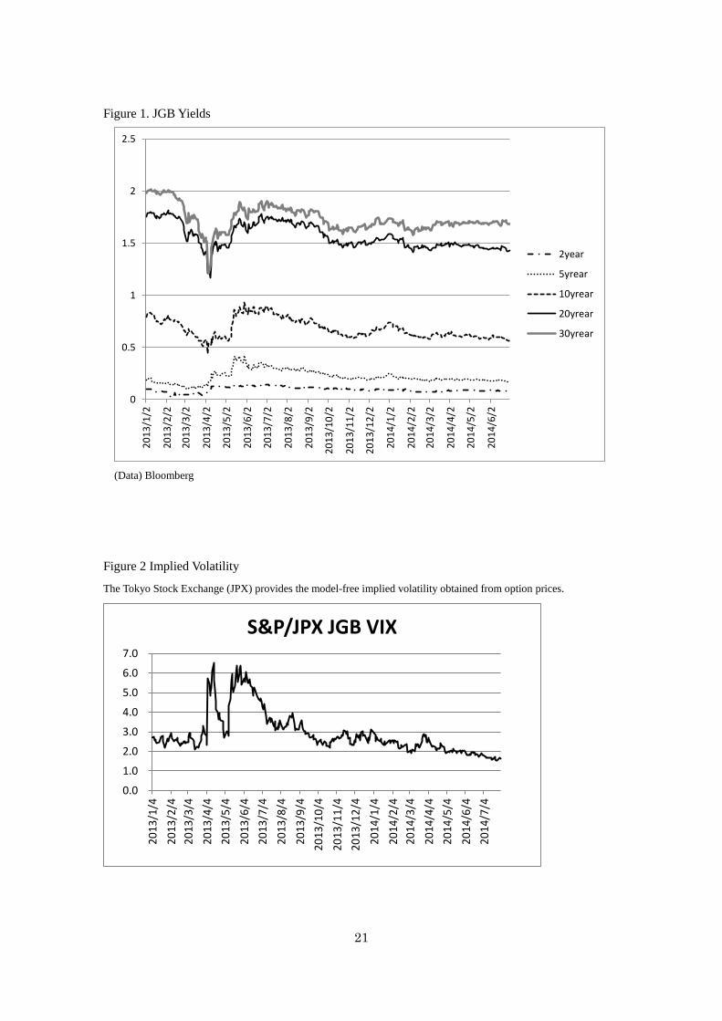
In addition, the implied volatility calculated from option prices of JGBs rose significantly

(Figure 2). The violent fluctuations in government bond prices continued from April into May,

during which the circuit breaker in the JGB futures market was triggered five times in

mid-April and further three times in May.

Possible side effects of large-scale government bond purchasing have been addressed by

many academician and central bankers. Former Federal Reserve Board Chairman Ben

Bernanke stated in his Jackson Hole speech that “if the Federal Reserve became too dominant

a buyer in a market, trading among private agents could dry up, degrading liquidity and price

discovery” (Bernanke, 2012).

Since the introduction of monetary easing, the Bank of Japan's bond holdings have exceeded

giant government bond holders, such as life and non-life insurance firms, due to their rapid

purchasing, resulting in a skewed bond distribution with a focus on 5- , 10- , 20- , and 30-year

newly issued bonds. Accordingly, the market participants became concerned over the possible

lack of floating government bonds in the market.

In general, does outright purchasing of government bonds by financial authorities deteriorate

market liquidity? Do conditions exist that can prevent this decrease? During and post the

second phase of the QQE policy, announced in October 2014, no confusion was evident, nor

was any anxiety around liquidity apparent during the first phase of the April 2013 monetary

easing. What was the difference?

While the motives and effectiveness of large-scale asset purchase programs have been

intensely debated, the effect of these trades on market quality has received much less attention.

Studies from the United States and European countries are split into two views: the theory that

a purchasing policy has a negative effect on market liquidity (Harvey and Huang, 2002;

3

Andersson, 2010; Inoue, 1999) and the theory that it improves market liquidity (Pasquariello,

et al., 2014; Brunetti et al., 2010; Christensen and Gillan, 2014). A consensus has not been

reached on this issue.

In this study, we show that the large change in the Bank of Japan's purchasing policy, since

the start of the monetary easing in April 2013, had an improved influence on market liquidity

in the government bond market, as evidenced by the decrease in quote spreads and Amihud’s

(2002) ILLIQ. The purchasing policy brought about three specific changes: 1) an increase in

the frequency of purchases; 2) a decrease in the purchase amount per transaction; and 3) a

decrease in the variability in the purchase amounts when purchased multiple times in one day.

We argue that these types of policy changes eased investors’ forecast on the purchasing

schedule and helped reduce market uncertainty. We find a significant rise in the adverse

selection component of the effective spread in response to the large-scale government bond

purchases right after the start of the QQE, but the impact gradually decreases and becomes

negative as the purchasing policy changes. The model free implied volatility also shows a

similar pattern. Together with the downward trend of the dispersion of the JGB yield forecasts

among market participants, these pieces of evidence support the theory that central banks’

communication and transparency play a significant role in the large-scale government bond

purchases in terms of market liquidity.

The rest of the paper is organized as follows. Section 2 provides a brief literature review and

a theoretical motivation for asymmetric information frameworks. Section 3 details the

execution of government bond purchases included in the QQE and Section 4 describes the

liquidity measures. Section 5 presents the empirical strategy and results. Section 6 discusses

the endogeneity issues and Section 7 concludes the paper.

2. Literature Review and Hypotheses

Although numerous studies have examined how open market operations (hereafter, OMOs),

a monetary policy used by financial authorities, affect asset value and the macroeconomy, few

studies have investigated its influence on financial market liquidity. Harvey and Huang’s

(2002) research appears to be the earliest study on the subject. Using intraday data on

government bond prices from 1982 to 1988, they show that the OMOs of the United States

increased the volatility of government bond prices. In subsequent studies, Andersson (2010)

confirms a strong upsurge in intraday bond market volatility at the time of the release of the

monetary policy decisions by the Federal Reserve Board, while Inoue (1999) discovers that

Japan’s OMOs increased the trade volume in the government bond market and the volatility of

government bond prices.

However, using data covering 2001 to 2007, Pasquariello et al. (2014) show that the OMOs

4

of the United States lowered the bid-ask spread and question the results of previous studies

claiming that monetary policies worsens market liquidity. In the paper, Pasquariello et al.

(2014) focus on the fact that FRB Chairman Alan Greenspan has made the FOMC increasingly

transparent by announcing the monetary policy intentions and disclosing the federal funds

target rate to the public. This change made OMOs virtually uninformative about the Federal

Reserve’s future monetary policy stance.

Among the recent growing literature on the large-scale asset purchase programs (LSAP),

Kandrac and Schlusche (2013) find no significant liquidity effects associated with Treasury

purchases. In contrast, Christensen and Gillan (2014) analyze the effect the Treasury

inflation-protected securities (TIPS) purchases, included in the Federal Reserve Board Q2

program, had on the functioning of the market for TIPS and the related market for inflation

swaps, and find that the liquidity premium is reduced due to the TIPS purchase.

In this way, it has not been settled whether OMOs worsen or improve government bond

market liquidity. First, let us briefly explain the theory that OMOs reduce market liquidity by

following Chari (2007). The basis of this theory is the adverse selection model, which is used

even in studies on central bank intervention in foreign exchange markets (Bhattacharya and

Weller, 1997; Naranjo and Nimalendran, 2000).

In the microstructure model with strategic informed traders, Chari (2007) assumes that

central banks are informed insiders since they have an informational advantage about the

fundamentals of government bond prices (Bhattacharya and Weller, 1997). Furthermore,

central banks have utility functions different from standard profit maximizing agents in that

they can choose to incur losses on their intervention operations. In doing so, central banks

weigh the expected cost of their bond transactions against their success in achieving target

objectives. On the other hand, rational speculators (i.e., strategic informed traders) in the

government bond market also have private information with respect to central bank objectives.

Furthermore, the following two conditions are set so that information may differ across

participants in the market when central banks intervene (Kyle, 1985; Bhattacharya and Speigel,

1991). First, central banks and speculators as a group can differ in their interpretation of the

fundamentals. Second, individual traders’ private signals about the fundamentals may differ

across traders. These two effects can lead to an increase in market uncertainty if the target price

implied by the intervention signal is not consistent with the fundamentals, causing speculators

facing the central bank’s transactions to trade more cautiously. As a result, uncertainty on the

future prices increases and market liquidity worsens. The uncertainty is especially intensified

when central bank interventions are unexpected. In such case, bid-ask spreads will increase due

to adverse selection risk and price volatility also increases.

Conversely, the theoretical model developed by Pasquariello et al. (2014) shows that the

5

OMOs improve market liquidity and the magnitude of this impact depends on the market’s

informational environment. The critical assumption of this theory is that, even though central

banks are informed traders facing a trade-off between policy motives (a non-public and

uninformed price target) and the expected cost of interventions, there is no information related

to the fundamentals in the OMOs. The reason is that they already release their monetary policy

decisions and policy details to the market before conducting OMOs. Therefore, the central

banks’ OMOs mitigate adverse selection concerns for market makers because they are noise

trades and thus induce speculators to trade more aggressively on their private signals, reducing

uncertainty about future prices. Consequently, price volatility decreases and the bid-ask spread

narrows.

The essential difference in assumptions between the two competing theories is whether

OMOs have any information on fundamentals. Japanese experience allows us to test these

theories since the Bank of Japan changed their JGB purchasing policy to enable traders to

forecast the timing and scale of OMOs and estimate fundamentals easily following the reduced

market liquidity experienced during the April 2013 monetary easing. The Bank of Japan made

their interventions more transparent by pre-announcing the monthly rough schedule of

purchases, increasing the frequency of trades and decreasing the purchase amount per

transaction. Therefore, we expect that government bond purchases do not worsen or even

improve market liquidity after the Bank of Japan changed their policy, as the theory by

Pasquariello et al. (2014) predicts.

3. Changes in the Bank of Japan’s Outright Purchasing Policy

With the aim of overcoming deflation that has lasted for nearly 15 years, the Bank of Japan

entered a new phase of monetary easing in terms of both quantity and quality in April 2013. It

began to double the monetary base and the amounts outstanding of JGBs as well as

exchange-traded funds (ETFs) in two years, and more than double the average remaining

maturity of JGB purchases. The Bank of Japan purchased JGBs from financial institutions in

the secondary market so that their amount outstanding increased at an annual rate of about 50

trillion yen1. In addition, the average remaining maturity of the Bank's JGB purchases was

extended from slightly less than three years to about seven years - equivalent to the average

maturity of the amount outstanding of JGBs issued.

However, the massive JGB purchases increased price volatility and worsened market

liquidity. The Bank of Japan responded to the market turbulence by changing the rate of its

1 The Bank of Japan increased the amount of purchases of JGBs at an annual rate of about 80

trillion yen at the start of the second phase of the QQE policy announced in October 2014.

6

purchases of government bonds. It increased the frequency of its purchases and lowered the

purchase amount per transaction. Table 1 shows that through these measures, the purchase

amount per transaction fell steadily from April 2014. The average number of purchases per day

was fixed at 2.6, the number of days on which bonds were purchased in a month at 10, and the

total number purchases in one month at 26 after June. Another apparent characteristic is that

the variability in the purchasing amount decreased then leveled off in cases where there were

multiple purchases in one day.

Furthermore, the Bank of Japan began to announce the monthly purchasing rate ex ante.

Although the detailed schedule of the Bank of Japan’s auctions is not disclosed in advance, a

broad pattern has been shared with market participants.

The following is an example of actual business procedures of OMOs. At 10:10 in the

morning, the Bank of Japan offers outright purchases of JBGs to eligible counterparties.

Around noon on the same day, it decides on the successful bids for the purchase and notifies

the bidders of the results on the total amounts of the bids, amounts of successful bids, and the

average successful bid rate via the Bank of Japan’s and others’ websites. The purchases are

executed generally two business days after the auction day.

We call the day when the target bond for outright purchasing and the purchase amount are

announced, “auction day,” and the day when the government bond purchase is executed,

“settlement day.” Since all the information about bond purchasing is revealed on the auction

days, it is expected that the impact on market liquidity occurs only on the auction days.

Since the frequency of OMOs has recently increased, it is often the case that the auction day

of new purchases coincides with the settlement day of the previous purchases. During the

sample period from April 4, 2013, to June 30, 2014, there are 307 business days. Among these

days, 74 days are when the auction day and the settlement day coincide.

4. Data

We measure liquidity using bid-ask spreads, effective spreads, one-minute realized spreads,

one-minute adverse selection, and Amihud’s (2002) ILLIQ.

Although the intraday data on the prices of the JGB futures traded on stock exchanges are

available, the intraday price data on over-the-counter trading of active JGBs (spot) are not

wholly available in Japan. Among various OTC brokers dealing with JGBs, the biggest broker,

Japan Bond Trading CO., Ltd. (BB), discloses only execution prices and yields, which makes it

impossible to measure liquidity. As an alternative to the broker’s data, we use intraday data

from Tradeweb, which is one of the top JGB brokers, operating electronic, over-the-counter

market places. The data is provided by Thomson Reuters and covers all bid and ask quotes.

Accordingly, we use the intraday quotes of 5- , 10- , 20- , and 30-year on-the-run JGBs to

7

calculate bid-ask spreads in the spot markets. These bonds reflect the type of long-term

maturity government bonds the Bank of Japan purchased.

We also measure liquidity in the JGB futures market by using the intraday data of the most

actively traded delivery month of JGB futures, particularly the long-term (10-year) government

bond futures, irrespectively the existence of 5- and 20- year bond futures. The data on JGB

futures, which are traded on Osaka Exchanges, are taken from Nikkei Media Marketing. It

includes all bid and ask prices, execution prices, and trading volume, which enables us to

calculate liquidity measures such as various spreads and ILLIQ.

Although intraday data is obtained, we do not focus on the intraday effect of OMOs on

liquidity because our preliminary analysis shows that the instantaneous impacts of the auction

announcements at 10:10 AM are neither significant nor stable. Instead, we analyze the effect

using the daily average of liquidity measures.

The bid-ask (half) spread is defined as

tttt mbidAskspreadaskbid 2/)(

where tm is the quote midpoint. The wider the bid-ask spread, the less liquid the government

bond. We use the daily averages of the spreads taken from one-minute intervals.

The effective (half) spread is defined as

ttttt mmpqspreadeffective /)(

where tq is an indicator variable that equals +1 for buyer-initiated trades and -1 for

seller-initiated trades, tp is the trade price, and tm is the quote midpoint prevailing at the

time of trade. We follow the standard trade-signaling approach of Lee and Ready (1991) and

use the contemporaneous quotes to sign trades and calculate effective spreads. For each day,

we use all JGB futures trades and quotes to calculate the average of all trades that day.

We also calculate Amihud's (2002) ILLIQ using the daily closing prices and daily trading

volume:

t

tt

volume

rILLIQ

|| .

If the effective spreads widen when JGBs are purchased, it is of interest to decompose the

spread along the lines of Glosten (1987) to determine whether the wider spread means

information asymmetry between informed traders and liquidity providers, or more revenue for

8

liquidity providers.

We estimate revenue to liquidity providers using the one-minute realized spread, which

assumes the liquidity provider is able to close her position at the quote midpoint one-minute

after the trade2. The realized spread is defined as

ttttt mmpqspreadrealized /)( 1

where 1tm is the quote midpoint one minute after the trade. In contrast, adverse selection is

measured using the one minute price impact of a trade, defined using the same variables as

ttttt mmmqselectionadverse /)( 1 .

Note that there is an arithmetic identity relating the realized spread, the adverse selection, and

the effective spread:

ttt selectionadversespreadrealizedspreadeffective .

In addition to asymmetric information, we use the dispersion of JGB yield forecasts among

traders as a measure of information heterogeneity and the implied volatility from option prices

as a measure of fundamental uncertainty. These three measures are expected to decrease if the

JGB purchasing policy change mitigates market uncertainty when the Bank of Japan intervenes

in the market.

The JGB yield forecasts are obtained from Quick Survey System (QSS), which conducts a

monthly paper-based survey of forecasts made by professional forecasters as well as their

attributes in Japanese financial markets. The number of respondents is between 130 and 150.

The implied volatility we use is the S&P/JPX VIX, which is provided by the Tokyo Stock

Exchange and it measures a 30-day forecast of the variability of the long-term (10-year) JGB

futures price.

Table 2 contains summary statistics and correlation coefficients for liquidity measures. There

are some points worth mentioning. First, on average the adverse selection is higher than the

realized spread. This is also evident from Figure 3. Both the bid-ask spreads and effective

spreads fluctuated unstably for some months from April 2013, but are stabilized afterwards.

The adverse selection is extremely high at the beginning of the sample period, while the

realized spread takes a negative value. This suggests that the degree of information asymmetry

2 We also analyzed using the same measures at five-minutes realized spreads and adverse

selection and obtained similar results to those one-minute measures.

9

is very high immediately after the QQE started. Further, the correlation between the adverse

selection and the realized spread is negative and close to -1.

Second, as Table 2 shows, the correlations between the Amihud’s (2002) ILLIQ and the

bid-ask spreads on spot and futures markets are positive and high, but the degree of

correlations are higher between JGB VIX and these spreads. Especially the VIX has high

correlations with the bid-ask spread and the effective spread on the futures market, whose

correlation coefficients are 0.86 and 0.78, respectively.

5. Estimation Results

In this section we analyze whether permanent OMOs generally reduce market liquidity and

what conditions prevent this decrease by utilizing the Bank of Japan’s outright JGB purchases.

We proceed in two steps. First, we test whether the change in purchasing policy by the Bank of

Japan contributes to improving market liquidity. Second, we test whether the change mitigates

the information asymmetry between informed traders and liquidity providers and thus

enhances market liquidity.

5-1. Outright JGB Purchases and Market Liquidity

We examine how the Bank of Japan’s purchasing policy had an effect on market liquidity as

their policy changed. To test this, we use an event study methodology following previous

literature (Andersen et al., 2003). Specifically, we set the auction day dummy (day t) and the

settlement day dummy (day t+2) as explanatory variables to compare the effects of bond

purchases; however, the effects may depend on the way that the Bank of Japan purchases.

Hence, we suppose that the coefficients of the auction and the settlement dummies are

dependent on the number of purchases in one day, the purchase amount per transaction, and the

standard deviation of the purchase amounts for one day.

Furthermore, we call the day adjacent to the auction day, “following day,” and include the

following day dummy (day t+1) as an additional explanatory variable to see if the impact on

liquidity lasts beyond a single day. We suppose that the effect of following day also depends on

variables related to the purchasing policy analogously.

Therefore, our estimation regression is as follows.

ti ititt

ttttt

edummydaySettlement

dummydayFollowingdummydayAuctionmeasureLiquidity

10

43

21

Xββ

ββα (1)

233232231303

123122121202

131211101

..

..

..

tttt

tttt

tttt

amountofdsamountaveragedayainnumber



where

βββββ

βββββ

βββββ

10

As liquidity indicators, we use the bid-ask half spreads for current 5- , 10- , 20- , and 30-year

bonds for JGB spot markets and the bid-ask spread, effective spread and ILLIQ for JGB futures.

As control variables, we enter a Bank of Japan policy meeting day dummy, a US Federal Open

Market Committee (FOMC) one-day lag dummy, and a Ministry of Finance (5-, 10-, 20-, and

30-year) tender day dummies. The lagged trading volume in the JGB futures market is also

included as a control variable, although the trading volume data is not available for the JGB

spot market.

Our analysis subject is confined to outright purchases of JGBs, excluding short-term

purchases such as those with sell-back conditions. We also exclude purchases of treasury

discount bills and the securities lending facility operation. The information on JGB auctions,

such as their schedule and volume, is obtained from the website of Tokyo Tanshi Corp.

As Table 2 shows, since a number of liquidity measures are serially correlated, we use

Newey-West estimators in OLS regressions to take into account autocorrelation and

heteroskedasticity in the error terms in the models.

Table 3 reports the results on the bid-ask spreads for 5-, 10-, 20-, and 30-year JGBs. The

estimated coefficients on the cross terms between the day dummies and the variables relating

to the purchasing policy indicate that increasing the frequency of purchases, decreasing the

amount, and leveling off the amounts lead to lower spreads, thus improving market liquidity

both on the auction and following days. The effect of lowering the amount continues to be

significant even on the settlement days. From the coefficients, it is evident that the impacts are

greater for longer maturity bonds. Table 4 shows that the bid-ask spread, the effective spread,

and ILLIQ for JGB futures are also sensitive to the change in purchasing policy. These results

suggest that the way the central bank intervenes has a significant bearing on market liquidity.

These effects do not die out only on the auction days but last at least three days until the

operations are executed.

In order to assess whether permanent OMOs improve or reduce market liquidity, we

calculate the time-varying coefficients representing the liquidity effect ( t1̂ , t2̂ , t3̂ in

Equation (1)) by exploiting the estimated coefficients obtained from the regressions and

monthly averages of the number of purchases in one day, the purchase amount per transaction,

and the standard deviation of the purchase amounts for one day. We rely on all estimated

coefficients even though they are not significant.

Figures 5 and 6 show the time-varying t̂ s from April 2013 to June 2014. All graphs show

that the impacts are positive and high in April 2013 and gradually shift downward. Second, it is

also clear that the impacts on some liquidity measures, such as the bid-ask spread and the

11

effective spreads, become negative in the latter half sub-sample period. Taking into account the

confidence interval, we find that the negative time-varying coefficients in the period are not

significantly different from zero, while those in the beginning of the sample period (from April

to May 2013) are significantly greater than zero3. Therefore, it is reasonable that the

purchasing policy changes contribute to improving liquidity to the degree that the JGB

purchases do not worsen the market liquidity. Lastly, the impact on liquidity is the highest on

the auction days, the second highest on the following days and the lowest on the settlement

days for the bid-ask spread, the effective spread, and ILLIQ.

5-2. The effects on asymmetric information, implied volatility, and dispersion of forecasts

We have shown that the Bank of Japan’s purchasing policy change has an improved

influence on market liquidity. However, what is the mechanism under which this policy change

works? Following the theories by Chari (2007) and Pasquariello et al. (2014), we argue that it

facilitates informed traders to forecast the time and scale of the next JGB purchases and to

estimate the fundamentals, and thus, mitigates market uncertainty so that they can further

engage in risk-arbitrage in the market.

To test this implication, we assess whether the following three variables are affected by the

Bank of Japan’s purchasing policy change: 1) the asymmetric information component of the

effective spread; 2) the implied volatility obtained from option prices; and 3) the dispersion of

forecasts on government bond yields. The asymmetric information and the implied volatility

are obtained on a daily basis, while the forecasts are collected on a monthly basis.

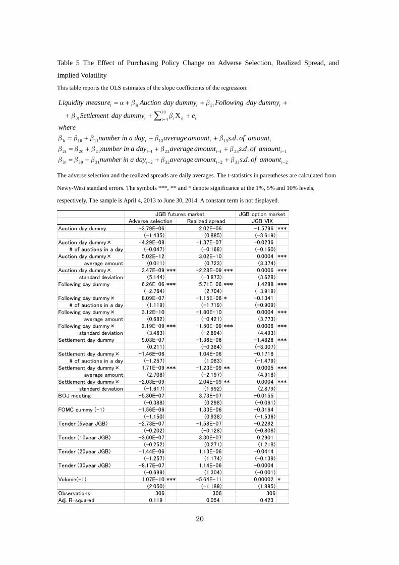
Table 5 reports the results of the regressions whose dependent variables are the adverse

selection, the realized spread, and the implied volatility. Leveling off the amount decreases the

adverse selection and increases the realized spread on the auction and following days. On the

other hand, a small amount interventions decrease the adverse selection on the settlement days.

For the implied volatility, a smaller amount and leveling off the amount decrease the implied

volatility on the auction, following, and settlement days.

In Figure 7, the graphs depict the time-varying coefficients of the three day dummies. The

adverse selection is positive and very high in April 2013 when intervening in the market, while

it becomes negative after September 2013. By contrast, the realized spread is negative but

becomes positive as time goes by. Both effects are evident on the auction and following days,

while the effect is not significant on the settlement days. In addition to this downward trend of

time-varying coefficients of the adverse selection, the effective spread and the adverse

selection has a high correlation (0.67), as shown at Table 2. The above evidence suggests that

3 The empirical results are not displayed in this paper but provided upon request.

12

the adverse selection is the key component in determining the effective spread.

The effect on the JGB VIX gradually becomes negative in March 2014. The impacts of the

three-day dummies are close to each other, but the magnitude is the highest on the auction days,

the second highest on the following days and lowest on the settlement days.

Since the forecasts on government bond yields are collected on a monthly basis, we are not

able to use the survey data in the regression analysis. However, Figure 8 shows that the

standard deviations of both 1-month and 3-month forecasts decline for 5-year, 10-year, and

20-year JGB yields. These pieces of evidence suggest that the Bank of Japan’s purchasing

policy change has a significant contribution to mitigating market uncertainty and enhancing

market liquidity.

6. Endogeneity Issues

A concern regarding the analysis presented above is the possibility that the purchases of JGBs

are endogenous. If the Bank of Japan reacts to worsening liquidity positions by purchasing

JGBs, then coefficient estimates will be biased. We conducted the Granger-causality using

daily data and found that JGB purchases are not caused by yesterday’s liquidity conditions4.

Another possibility is that the Bank of Japan may respond to market liquidity on an intraday

basis. However, this is impractical as purchases are relatively large, occur early in the morning,

and would require a simultaneous response to many different liquidity indicators.

Another concern is that if the purchasing policy change enables traders to forecast the next

intervention exactly, the purchasing day dummies become endogenous. In practice, however,

what the Bank discloses is not the detailed schedule of purchases but rather a monthly rough

schedule. Therefore, the exact timing and size of interventions remains uncertain for traders

when the Bank intervenes in the market.

7. Conclusion

In this study, we investigate how the Bank of Japan’s outright JGB purchases has an effect

on market liquidity. Although there are the two opposing theories on the effect, their critical

differences are whether OMOs have any information related to fundamentals. The large change

in the Bank of Japan's purchasing policy after the monetary easing in April 2013 is a natural

experiment to allow us to test the implication from the theories. The purchasing policy brought

about three specific changes: 1) an increase in the frequency of purchases; 2) a decrease in the

purchase amount per transaction; and 3) a decrease in the variability in the purchase amounts

when purchased multiple times in one day. These types of policy changes eased investors’

4 The empirical results are not displayed in this paper but provided upon request.

13

expectations on the schedule of the next purchases and their estimations of the fundamentals,

reducing market uncertainty. The regression results show that these policy changes

significantly contributed to the improvement of the market liquidity. In addition, the adverse

selection, the implied volatility, and the dispersion of forecasts are all reduced by the policy

change. These pieces of evidence suggest that central banks’ communication and transparency

play an important role in the large-scale government bond purchases in terms of market

liquidity.

Appendix

We thank Takasi Hatakeda, Kazuhito Ikeo, Bernd Hayo, Kazuhiko Ohashi, Wataru Ohta,

Paolo Pasquariello, Jie Qin, Ghon Rhee, Toshio Serita, Hideki Takada, Toyoharu Takahash,

Yasuhiko Tanigawa, Kazuo Ueda, Toshiaki Watanabe, Toshinao Yoshiba, and seminar

participants at the Bank of Japan Finance Workshop, University of Hawaii, the 11th

International Conference on Asian Financial Markets and Economic Development at Nagasaki

University, and Asian Finance Association Meeting. We are also grateful to Editage for English

language editing. This work was supported by JSPS KAKENHI Grant Number 16K03742.

14

References

Amihud, Y. (2002). Illiquidity and stock returns: Cross-section and time series effects, Journal

of Financial Markets, 5, 31–56.

Andersen, T. G., Bollerslev, T. O., Diebold, F. X., and Vega, C. (2003). Micro Effects of Macro

Announcements: Real-Time Price Discovery in Foreign Exchange, American Economic

Rerview, 93,1, 38-62.

Andersson, M. (2010). Using intraday data to gauge financial market responses to Federal

Reserve and ECB monetary policy decisions, International Journal of Central Banking, 6,

2, 117-146.

Bernanke, S. B. (2012), Monetary Policy since the Onset of the Crisis. Remarks at the Federal

Reserve Bank of Kansas City Economic Symposium, Jackson Hole, Wyoming, August 31,

http://www.federalreserve.gov/newsevents/speech/bernanke20120831a.pdf

Bhattacharya, U. and M. Spiegel (1991). Insiders, Outsiders and Market Breakdowns, Review

of Financial Studies, 4, 255-282.

Bhattacharya, U. and P. Weller (1997). The advantage to hiding one’s hand: speculation and

central bank intervention in the foreign exchange market, Journal of Monetary Economics,

39, 251-277.

Brunetti, C., M. Filippo, and J. H. Harris (2010). Effects of central bank intervention on the

interbank market during the subprime crisis, Review of Financial Studies, 24, 6,

2053-2083.

Chari., A. (2007). Heterogeneous market-making in foreign exchange markets: evidence from

individual bank responses to central bank interventions, Journal of Money, Credit and

Banking, 39,5, 1131-1161.

Christensen, J. H. E. and J. M. Gillan. (2014). Does quantitative easing affect market liquidity?,

Federal Reserve Bank of San Francisco Working Paper Series, 2013-26.

Glosten, L. R. (1987). Components of the bid ask spread and the statistical properties of

transaction prices, Journal of Finance 42, 1293-1307.

Harvey, R. C. and R. D. Huang. (2002). The impact of the Federal Reserve Bank’s open market

operations, Journal of Financial Markets, 5, 223-257.

Inoue, H. (1999). The effects of open market operations on the price discovery process in the

Japanese government securities market: an empirical study, Working Paper.

https://www.bis.org/publ/cgfs11ino_c.pdf

Kandrac, J. and B. Schlusche (2014). Flow effects of large-scale asset purchases, Economics

Letters 121, 330-335.

Kyle, A. S. (1985). Continuous Auction and Insider Trading, Econometrica, 53, 1315-1385.

http://www.federalreserve.gov/newsevents/speech/bernanke20120831a.pdf

https://www.bis.org/publ/cgfs11ino_c.pdf

15

Lee, C. M. C., and M. J. Ready (1991). Inferring trade direction from intraday data, Journal of

Finance 46, 733-746.

Naranjo, A. and M. Nimalendran (2000). Government Intervention and adverse selection costs

in foreign exchange markets, Journal of Finance, 13, 2, 453-477.

Pasquariello, P., J. Roush, and C. Vega (2014). Government intervention and strategic trading

in the U.S. treasury market, Working Paper, University of Michigan.

http://webuser.bus.umich.edu/ppasquar/openmarket.pdf

http://webuser.bus.umich.edu/ppasquar/openmarket.pdf

16

Table 1 Changes of Purchasing Strategy of JGB

The units are the number of times, and billion yen. The data is from the website of the Tokyo

Tanshi Corp.

(times, billion yen)

Date of auctionsAveragenumberin a day

Average daysin a month

Averagenumber ina month

Averageamount pertransaction

Amount ina month

Average of standarddeviation of amountin a day

Jan.-March　2013 2.00 4.0 8.0 2,181 17,448 527April 2.50 6.0 15.0 4,426 68,146 1,784May 2.29 7.0 16.0 4,146 65,450 1,690June 2.60 10.0 26.0 3,208 81,709 1,314July 2.60 10.0 26.0 2,716 71,015 1,173August 2.60 10.0 26.0 2,791 71,720 951September 2.60 10.0 26.0 2,853 74,025 917October 2.60 10.0 26.0 2,851 75,262 768November 2.60 10.0 26.0 2,724 72,035 847December 2.60 10.0 26.0 2,626 68,228 714Jan.-June　2014 2.63 10.0 26.3 2,445 65,368 734

17

Table 2 Descriptive Statistics and Correlation Coefficients

This table reports summary statistics for liquidity measures and others from April 4, 2013 to June 30, 2014. Spreads are all unit-free as they are divided by the midquote. The unit of

the JGB VIX is percentage (%). The JGB VIX meaures the market estimate of the price fluctuation of 10-year JGB Futures over the next 30 days.

JGB OptionBid-ask spread(5 year)

Bid-ask spread(10 year)



Bid-ask spread Effective spread ILLIQ Adv. selection Realized spread VIX

Mean 0.00030 0.00059 0.00152 0.00181 0.00004 0.00004 4.05E-08 0.00002 0.00001 3.083 Median 0.00030 0.00058 0.00152 0.00171 0.00004 0.00004 2.84E-08 0.00002 0.00001 2.680 Maximum 0.00039 0.00094 0.00207 0.00274 0.00005 0.00005 3.10E-07 0.00008 0.00002 6.550 Minimum 0.00016 0.00040 0.00087 0.00102 0.00003 0.00003 0.00E+00 0.00001 -0.00003 1.730 Std. Dev. 0.00003 0.00007 0.00021 0.00036 2.45E-06 1.65E-06 4.06E-08 5.84E-06 4.89E-06 1.154 Skewness -0.21506 0.96051 -0.34359 0.80043 2.51802 3.74181 2.17899 3.88369 -2.92610 1.28917 Kurtosis 3.4663 6.3235 3.5283 3.1120 9.8936 24.1694 10.7157 32.6192 22.4761 3.6715 Autocorr. 0.6860 0.6040 0.7860 0.8480 0.7880 0.6490 0.1420 0.2020 0.0990 0.9520 Observations 307 307 307 307 307 307 307 307 307 307Bid-ask (5 yr) 1.000Bid-ask (10yr)

0.187 1.000

Bid-ask (20yr)

0.347 0.522 1.000

Bid-ask (30yr)

0.225 0.453 0.667 1.000

Bid-ask(Futures)

-0.046 -0.151 -0.179 -0.172 1.000

Effectivespred (futures)

0.348 0.222 0.383 0.265 0.903 1.000

ILLIQ (futures) 0.193 0.228 0.283 0.265 0.348 0.432 1.000Adv. Selection(futures)

0.204 0.124 0.274 0.203 0.520 0.669 0.308 1.000

Realized sp.(futures)

-0.126 -0.074 -0.198 -0.153 -0.317 -0.461 -0.221 -0.968 1.000

JGB VIX 0.427 0.312 0.488 0.400 0.856 0.777 0.392 0.378 -0.190 1.000

JGB spot JGB futures

18

Table 3 The Effect of Purchasing Policy Change (JGB Spot)

This table reports the OLS slope coefficients of the following regression with the daily average of bid-ask spreads

for the on-the-run JGBs:

233232231303

123122121202

131211101

9

43

21

..

..

..

X

tttt

tttt

tttt

ti ititt

ttttt




where

edummydaySettlement


βββββ

βββββ

βββββ

ββ

ββα

The t-statistics in parentheses are calculated from Newy-West standard errors. The symbols ***, ** and * denote

significance at the 1%, 5% and 10% levels, respectively. The sample is April 4, 2013 to June 30, 2014. A constant

term is not displayed.

5 years 10 years 20 years 30 yearsAuction day dummy 1.24E-05 -1.25E-05 -2.91E-04 *** -1.81E-04

(0.870) (-0.372) (-4.442) (-1.182)

Auction day dummy× -8.18E-06 * -1.54E-05 -4.90E-05 * -6.49E-05# of auctions in a day (-1.814) (-1.315) (-1.769) (-1.303)

Auction day dummy× 8.18E-10 1.24E-08 * 6.67E-08 *** 1.64E-07 ***average amount (0.197) (1.648) (3.426) (4.530)

Auction day dummy× 9.90E-09 *** 1.11E-08 *** 6.61E-08 *** 1.28E-08standard deviation (2.288) (2.408) (2.859) (0.316)

Following day dummy 2.19E-05 -1.90E-05 -3.33E-04 *** -3.19E-04 **(1.448) (-0.463) (-4.621) (-2.216)

Following day dummy× -1.59E-05 *** -5.73E-06 5.93E-05 ** -2.75E-05# of auctions in a day (-3.297) (-0.482) (2.166) (-0.536)

Following day dummy× 6.37E-09 * 6.86E-09 6.84E-08 *** 1.55E-07 ***average amount (1.851) (0.779) (3.333) (3.943)

Following day dummy× 9.33E-09 ** 7.77E-09 6.69E-08 *** 3.10E-08standard deviation (2.052) (0.970) (2.922) (0.704)

Settlement day dummy -1.23E-05 -2.72E-05 -2.87E-04 *** -3.06E-04(-0.846) (-0.942) (-3.631) (-2.292)

Settlement day dummy× -4.42E-06 -1.35E-05 * 1.72E-05 -3.71E-05# of auctions in a day (-1.188) (-1.704) (0.649) (-0.877)

Settlement day dummy× 1.00E-08 *** 2.41E-08 *** 9.25E-08 *** 1.56E-07 ***average amount (3.016) (3.384) (4.341) (4.244)

Settlement day dummy× -5.97E-10 -7.49E-09 3.26E-08 5.25E-10standard deviation (-0.136) (-0.655) (1.334) (0.011)

BOJ meeting -6.29E-07 2.25E-06 4.65E-06 4.31E-05(-0.064) (0.123) (0.116) (0.617)

FOMC dummy (-1) -1.91E-05 * -5.75E-06 -2.16E-05 -8.89E-05(-1.659) (-0.349) (-0.355) (-1.154)

Tender (5year JGB) -5.75E-06 1.31E-05 1.39E-04 *** 6.33E-05(-0.702) (0.547) (3.381) (0.587)

Tender (10year JGB) 1.23E-05 1.87E-05 9.31E-05 ** 1.80E-04 ***(1.463) (1.264) (2.311) (2.678)

Tender (20year JGB) -1.43E-05 -9.66E-06 9.17E-05 -3.41E-05(-1.241) (-0.528) (1.496) (-0.399)

Tender (30year JGB) 1.48E-05 -1.75E-05 5.48E-05 1.17E-04(1.861) (-0.878) (0.867) (1.085)

Observations 307 307 307 307Adj. R-squared 0.053 0.057 0.203 0.145

Bid-ask spreads of JGB spot markets

19

Table 4 The Effect of Purchasing Policy Change (JGB Futures)

This table reports the OLS slope coefficients of the following regression of daily liquidity measures for JGB futures:

233232231303

123122121202

131211101

10

43

21

..

..

..

X

tttt

tttt

tttt

ti ititt

ttttt




where

edummydaySettlement


βββββ

βββββ

βββββ

ββ

ββα

The bid-ask spreads are calculated by taking the 1 min. average of the bid-ask spreads. The effective spread is the

daily average. ILLIQ is Amihud’s (2002) illiquidity measure. The t-statistics in parentheses are calculated from

Newy-West standard errors. The symbols ***, ** and * denote significance at the 1%, 5% and 10% levels,

respectively. The sample is April 4, 2013 to June 30, 2014. A constant term is not displayed.

Auction day dummy -3.00E-06 *** -1.77E-06 *** -6.93E-08 ***(-3.362) (-2.899) (-3.277)

Auction day dummy× -1.86E-07 -1.80E-07 -1.34E-08 *# of auctions in a day (-0.560) (-0.818) (-1.747)

Auction day dummy× 5.60E-10 ** 3.07E-10 ** 7.92E-12 **average amount (2.409) (2.070) (2.061)

Auction day dummy× 1.99E-09 *** 1.19E-09 *** 1.07E-11 **standard deviation (5.321) (5.267) (1.990)

Following day dummy -1.83E-06 * -5.52E-07 -1.56E-08(-1.868) (-0.920) (-0.718)

Following day dummy× -3.93E-07 -3.44E-07 * -4.05E-09# of auctions in a day (-1.224) (-1.776) (-0.598)

Following day dummy× 5.01E-10 ** 1.32E-10 6.25E-12average amount (2.067) (0.903) (1.254)

Following day dummy× 1.15E-09 *** 6.90E-10 *** 6.69E-12standard deviation (3.653) (3.670) (1.002)

Settlement day dummy -1.57E-06 -4.56E-07 -3.08E-08 *(-1.579) (-0.443) (-1.750)

Settlement day dummy× -4.14E-07 * -4.12E-07 -2.61E-09# of auctions in a day (-1.639) (-1.586) (-0.552)

Settlement day dummy× 7.74E-10 *** 4.77E-10 *** 1.19E-11 **average amount (3.091) (3.225) (2.514)

Settlement day dummy× 3.45E-10 1.18E-11 7.72E-14standard deviation (1.214) (0.038) (0.014)

BOJ meeting dummy 4.51E-08 -1.57E-07 -9.17E-09(0.090) (-0.438) (-1.006)

FOMC dummy (-1) -3.89E-07 -2.31E-07 5.35E-09(-0.658) (-0.657) (0.499)

Tender (5year JGB) -1.68E-07 -4.31E-07 1.63E-08(-0.240) (-1.474) (1.120)

Tender (10year JGB) 1.84E-07 -2.99E-08 -1.02E-08(0.476) (-0.087) (-1.215)

Tender (20year JGB) -5.05E-07 -3.10E-07 3.00E-09(-1.069) (-0.936) (0.320)

Tender (30year JGB) 5.73E-07 3.20E-07 -1.56E-08 **(0.593) (0.578) (-2.057)

Volume(-1) 6.8E-11 *** 5.08E-11 *** -7.91E-14(2.757) (2.877) (-0.207)

Observations 306 306 306Adj. R-squared 0.362 0.280 0.075

JGB futures marketBid-ask spread Effective spread ILLIQ

20

Table 5 The Effect of Purchasing Policy Change on Adverse Selection, Realized Spread, and

Implied Volatility

This table reports the OLS estimates of the slope coefficients of the regression:

233232231303

123122121202

131211101

10

43

21

..

..

..

X

tttt

tttt

tttt

ti ititt

ttttt




where

edummydaySettlement


βββββ

βββββ

βββββ

ββ

ββα

The adverse selection and the realized spreads are daily averages. The t-statistics in parentheses are calculated from

Newy-West standard errors. The symbols ***, ** and * denote significance at the 1%, 5% and 10% levels,

respectively. The sample is April 4, 2013 to June 30, 2014. A constant term is not displayed.

Auction day dummy -3.79E-06 2.02E-06 -1.5796 ***(-1.435) (0.885) (-3.619)

Auction day dummy× -4.29E-08 -1.37E-07 -0.0236# of auctions in a day (-0.047) (-0.168) (-0.160)

Auction day dummy× 5.02E-12 3.02E-10 0.0004 ***average amount (0.011) (0.723) (3.374)

Auction day dummy× 3.47E-09 *** -2.28E-09 *** 0.0006 ***standard deviation (5.144) (-3.873) (3.628)

Following day dummy -6.26E-06 *** 5.71E-06 *** -1.4288 ***(-2.764) (2.704) (-3.919)

Following day dummy× 8.09E-07 -1.15E-06 * -0.1341# of auctions in a day (1.119) (-1.719) (-0.909)

Following day dummy× 3.12E-10 -1.80E-10 0.0004 ***average amount (0.682) (-0.421) (3.773)

Following day dummy× 2.19E-09 *** -1.50E-09 *** 0.0006 ***standard deviation (3.463) (-2.694) (4.493)

Settlement day dummy 9.03E-07 -1.36E-06 -1.4826 ***(0.211) (-0.384) (-3.307)

Settlement day dummy× -1.46E-06 1.04E-06 -0.1718# of auctions in a day (-1.257) (1.083) (-1.479)

Settlement day dummy× 1.71E-09 *** -1.23E-09 ** 0.0005 ***average amount (2.708) (-2.197) (4.918)

Settlement day dummy× -2.03E-09 2.04E-09 ** 0.0004 ***standard deviation (-1.617) (1.992) (2.879)

BOJ meeting -5.30E-07 3.73E-07 -0.0155(-0.388) (0.298) (-0.061)

FOMC dummy (-1) -1.56E-06 1.33E-06 -0.3164(-1.150) (0.938) (-1.536)

Tender (5year JGB) -2.73E-07 -1.58E-07 -0.2282(-0.202) (-0.128) (-0.808)

Tender (10year JGB) -3.60E-07 3.30E-07 0.2901(-0.252) (0.271) (1.218)

Tender (20year JGB) -1.44E-06 1.13E-06 -0.0414(-1.257) (1.174) (-0.139)

Tender (30year JGB) -8.17E-07 1.14E-06 -0.0004(-0.699) (1.304) (-0.001)

Volume(-1) 1.07E-10 *** -5.64E-11 0.00002 *(2.050) (-1.189) (1.895)

Observations 306 306 306Adj. R-squared 0.119 0.054 0.423

JGB futures market JGB option marketAdverse selection Realized spread JGB VIX

21

Figure 1. JGB Yields

(Data) Bloomberg

Figure 2 Implied Volatility

The Tokyo Stock Exchange (JPX) provides the model-free implied volatility obtained from option prices.

0

0.5

1

1.5

2

2.52

01

3/1

/2

20

13

/2/2

20

13

/3/2

20

13

/4/2

20

13

/5/2

20

13

/6/2

20

13

/7/2

20

13

/8/2

20

13

/9/2

20

13

/10

/2

20

13

/11

/2

20

13

/12

/2

20

14

/1/2

20

14

/2/2

20

14

/3/2

20

14

/4/2

20

14

/5/2

20

14

/6/2

2year

5yrear

10yrear

20yrear

30yrear

0.0

1.0

2.0

3.0

4.0

5.0

6.0

7.0

20

13

/1/4

20

13

/2/4

20

13

/3/4

20

13

/4/4

20

13

/5/4

20

13

/6/4

20

13

/7/4

20

13

/8/4

20

13

/9/4

20

13

/10

/4

20

13

/11

/4

20

13

/12

/4

20

14

/1/4

20

14

/2/4

20

14

/3/4

20

14

/4/4

20

14

/5/4

20

14

/6/4

20

14

/7/4

S&P/JPX JGB VIX

22

Figure 3 Comparison of Spreads and Spread Components

(Data) The JGB futures price and volume data are from Nikkei Media Marketing

Figure 4 Amihud’s (2002) Illiquidity Measure, ILLIQ

(Data) The JGB futures price and volume data are from Nikkei Media Marketing

-4.0E-05

-2.0E-05

0.0E+00

2.0E-05

4.0E-05

6.0E-05

8.0E-05

1.0E-04

20

13

/4/1

20

13

/6/1

20

13

/8/1

20

13

/10

/1

20

13

/12

/1

20

14

/2/1

20

14

/4/1

20

14

/6/1

bid-ask spread

effective spread

adverse selection

realized spread

0.0E+00

5.0E-08

1.0E-07

1.5E-07

2.0E-07

2.5E-07

3.0E-07

3.5E-07

20

13

/4/1

20

13

/5/1

20

13

/6/1

20

13

/7/1

20

13

/8/1

20

13

/9/1

20

13

/10

/1

20

13

/11

/1

20

13

/12

/1

20

14

/1/1

20

14

/2/1

20

14

/3/1

20

14

/4/1

20

14

/5/1

20

14

/6/1

ILLIQ

23

Figure 5 Liquidity Impacts of Interventions in the JGB Spot Market

(5-, 10-, 20-, 30-Year JGBs)

233232231303

123122121202

131211101

9

43

21

..

..

..

X

tttt

tttt

tttt

ti ititt

ttttt




where

edummydaySettlement

dummydayFollowingdummydayAucitonmeasureLiquidity

βββββ

βββββ

βββββ

ββ

ββα

These graphs show the time-varying coefficient of the auction day dummy ( t1̂ ), that of the following day dummy

( t2̂ ), and that of the settlement day dummy ( t3̂ ). These coefficients are calculated with the regression estimates

and the monthly averages of the number of purchases in a day, the monthly averages of the purchasing amount and

the monthly average of the standard deviation of the daily amounts.

-1.0E-04

0.0E+00

1.0E-04

2.0E-04

3.0E-04

4.0E-04

5 year JGB

Auciton day impact Following day impact Settlement day impact

-1.0E-04

0.0E+00

1.0E-04

2.0E-04

3.0E-04

4.0E-04

10 year JGB


-1.0E-04

0.0E+00

1.0E-04

2.0E-04

3.0E-04

4.0E-04

20 year JGB


-1.0E-04

0.0E+00

1.0E-04

2.0E-04

3.0E-04

4.0E-04

30 year JGB


24

Figure 6 Liquidity Impacts of Interventions in the JGB Futures Market

(Bid-ask Spread, Effective Spreads, ILLIQ)

233232231303

123122121202

131211101

10

43

21

..

..

..

X

tttt

tttt

tttt

ti ititt

ttttt




where

edummydaySettlement

dummydayFollowingdummydayAucitonmeasureLiquidity

βββββ

βββββ

βββββ

ββ

ββα





-2.0E-06

-1.0E-06

0.0E+00

1.0E-06

2.0E-06

3.0E-06

4.0E-06

5.0E-06

Bid-ask spread


-2.0E-06

-1.0E-06

0.0E+00

1.0E-06

2.0E-06

3.0E-06

4.0E-06

5.0E-06

Effective spread


-1.0E-08

0.0E+00

1.0E-08

2.0E-08

3.0E-08

4.0E-08

ILLIQ


25

Figure 7 Impacts of Interventions in the Futures and Option Markets

(Adverse Selection, Realized Spreads, JGB VIX)

233232231303

123122121202

131211101

10

43

21

..

..

..

X

tttt

tttt

tttt

ti ititt

ttttt




where

edummydaySettlement

dummydayFollowingdummydayAucitonMeasure

βββββ

βββββ

βββββ

ββ

ββα





-3.0E-06

-2.0E-06

-1.0E-06

0.0E+00

1.0E-06

2.0E-06

3.0E-06

4.0E-06

5.0E-06

Adverse selection


-3.0E-06

-2.0E-06

-1.0E-06

0.0E+00

1.0E-06

2.0E-06

3.0E-06

4.0E-06

5.0E-06

Realized spread


-0.5

0.0

0.5

1.0

1.5

2.0

2.5

JGB VIX


26

Figure 8 Dispersion of JGB Yield Forecasts among Traders

The below graphs depict the standard deviations of one-month and three-month forecasts for 5-, 10-, and 20-year

JGB yields. The Quick Survey System (QSS) conducts a monthly paper-based survey of forecasts made by

professional forecasters as well as their attributes in Japanese financial markets. The number of respondents is

between 130 and 150.

0

0.02

0.04

0.06

0.08

0.1

0.12

0.14

0.16

0.18

20

13

/01

20

13

/02

20

13

/03

20

13

/04

20

13

/05

20

13

/06

20

13

/07

20

13

/08

20

13

/09

20

13

/10

20

13

/11

20

13

/12

20

14

/01

20

14

/02

20

14

/03

20

14

/04

20

14

/05

20

14

/06

%S.D. of 1 month forecasts

5 year JGB

10 year JGB

20 year JGB

0

0.02

0.04

0.06

0.08

0.1

0.12

0.14

0.16

0.18

20

13

/01

20

13

/02

20

13

/03

20

13

/04

20

13

/05

20

13

/06

20

13

/07

20

13

/08

20

13

/09

20

13

/10

20

13

/11

20

13

/12

20

14

/01

20

14

/02

20

14

/03

20

14

/04

20

14

/05

20

14

/06

S.D. of 3 month forecasts

5 year JGB

10 year JGB

20 year JGB

quantitative easing and liquidity in the japanese ...1 quantitative easing and liquidity in the...

Documents