Department of Physics and Measurement Technology

Final Thesis

Quantitative analysis of multi-phase systems -steels with mixture of ferrite and austenite

Fawad Salman Khokhar

LITH-IFM-EX--04/1358--SE

Linköping UniversityInstitute of Technology

Department of Physics and Measurement Technology

Linköping University

SE-581 83 Linköping, Sweden

2

Linköping University Institute of Technology

Final Thesis

Fawad Salman Khokhar

LITH-IFM-EX--04/1358—SE Department of Physics and Measurement Technology

Linköping University, Sweden

Sandvik Materials Technology

3

Supervisor: Dr. Ping Liu Senior Scientist

R & D, Sandvik Materials Technology Sandviken, Sweden

Examiner: Prof. Leif Johansson Department of Physics and Measurement Technology

Linköping University, Sweden

4

“The difference between stupidity and genius is that genius has its limits.”

-Albert Einstein (1879-1955)

5

Acknowledgement

I would like to thank every one who has supported me during this project work.

The entire staff at the Dept. of Physical Metallurgy at Sandvik Materials Technology deserves

profound compliments for providing friendly environment to work in. I would like to thank Dr.

Yang Yu at Höganäs AB for providing specimens for this project. I would also like to express

gratitude to my examiner Prof. Leif I. Johansson at Dept. of Physics and Measurement

Technology, Linköping University.

Last but not least, I am sincerely grateful to my supervisor Dr. Ping Liu for all his help,

supervision, precious advice and discussions at each and every stage of this project work.

Fawad Salman Khokhar

January 2005.

6

Abstract The goal of this diploma work has been to evaluate the different experimental techniques used

for quantitative analysis of multi-phase materials systems.

Powder based specimens containing two-phases, austenite (γ) and ferrite (α), were fabricated

and quantified. The phase volume fraction of ferrite varied from 2 Vol% to 50 Vol%.

X-ray powder diffraction (XRD) measurements were based on two peak analysis. Computer

based software Topas was used for quantitative analysis, which is believed to be the most

advanced in this field. XRD results were found within the absolute limit of ± 4% of given

ferrite volume fraction. Volume fraction as low as 2 Vol% was successfully detected and

quantified using XRD. However, high statistical error was observed in case of low volume

fraction, such as 2 Vol% and 5 Vol% ferrite volume fraction.

Magnetic balance (MB) measurements were performed to determine the volume fraction of

magnetic phase, ferrite. MB results were found in good agreement with given volume fractions.

As low as 2 Vol% volume phase fraction was detected and quantified with MB. MB results

were within the absolute limit of ± 4% of given ferrite volume fraction.

Image analysis (IA) was performed after proper sample preparation as required by electron

backscatter diffraction (EBSD) mode of Scanning electron microscopy (SEM). IM results were

found within the absolute limit of ± 2 % of given ferrite volume fraction. However, high

statistical error was observed in case of 2 Vol% volume fraction.

7

Contents Acknowledgement ................................................................................................................................... 5 Abstract..................................................................................................................................................... 6

Contents ........................................................................................................................................... 7

Introduction................................................................................................................................... 10

Chapter One .................................................................................................................................. 11 Two phase materials and the importance of quantification............................................................. 11

1.1.1 Piezoelectric and Pyroelectric Properties ..............................................................................................11 1.1.2 Insulate –metal Behavior .........................................................................................................................12 1.1.3 Fatigue Strength........................................................................................................................................12 1.1.4 Toughness of two-phase ceramics ...........................................................................................................13 1.1.5 Mechanical Properties..............................................................................................................................13

1.2 Duplex Stainless Steels .................................................................................................................... 14 1.2.1 Mechanical Strength.................................................................................................................................14 1.2.2 Toughness ..................................................................................................................................................15

Transition temperature....................................................................................................................................15 1.2.3 Corrosion ...................................................................................................................................................15 1.2.4 Hydrogen Embrittlement.........................................................................................................................16

1.3 Importance of quantification ......................................................................................................... 17 1.4 Fabrication of specimens ................................................................................................................ 18

Austenite powder (316L SS) .............................................................................................................................18 Iron powder (ASC100.29) .................................................................................................................................18

Chapter Two .................................................................................................................................. 19 Experimental techniques ...................................................................................................................... 19 2.1 X-Ray powder Diffraction (XRD) ................................................................................................. 19

XRD principle.....................................................................................................................................................19 Diffraction Methods...........................................................................................................................................21 Illustration of X-ray Powder Diffractrometer................................................................................................22 X ray diffraction intensity.................................................................................................................................23 2.1.1 Quantitative phase analysis by X- ray powder diffraction ................................................................24

Quantitative Methods......................................................................................................................................25 Experimental limitations.................................................................................................................................27 Practical Difficulties .......................................................................................................................................27

Preferred Orientation .................................................................................................................................27 Microabsorption.........................................................................................................................................28 Extinction ...................................................................................................................................................28

2.1.2 Statistical Error.........................................................................................................................................28 2.1.2 Full-Pattern phase quantification ...........................................................................................................29

2.2 Magnetic Balance ............................................................................................................................ 30 Theory .................................................................................................................................................................30 Calculation of magnetic phase..........................................................................................................................31 Source of error ...................................................................................................................................................32

8

2.3 Image Analysis ................................................................................................................................. 33 2.3.1 Procedure of image analysis........................................................................................................ 33

Image acquisition ............................................................................................................................................33 The Grey image processing ............................................................................................................................34 Thresholding and Binary image processing ...................................................................................................34

2.3.2 Possible errors ...........................................................................................................................................34 Scanning Electron Microscope.........................................................................................................................35

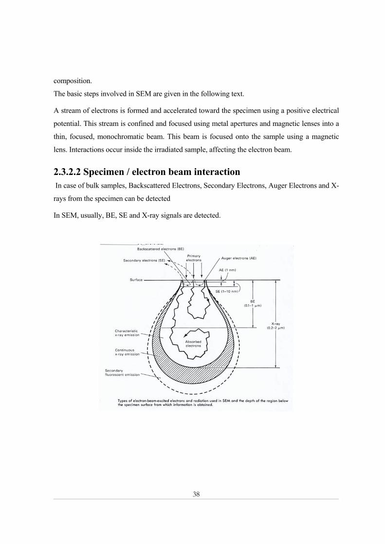
2.3.2 Scanning Electron Microscope ................................................................................................... 36 Morphology.....................................................................................................................................................36 Crystallographic Information..........................................................................................................................36 Composition....................................................................................................................................................36

2.3.2.1 Operations ..............................................................................................................................................36 Electron source................................................................................................................................................36 Electromagnetic lens and Aperture ................................................................................................................37 Vacuum in SEM..............................................................................................................................................37 Specimen Preparation .....................................................................................................................................37 How SEM works.............................................................................................................................................37

2.3.2.2 Specimen / electron beam interaction .................................................................................................38 2.3.3 Electron backscatter diffraction............................................................................................... 39

Principle ..............................................................................................................................................................39 Automated indexing...........................................................................................................................................41 EBSD Mapping ..................................................................................................................................................43 Instrumentation..................................................................................................................................................43 Sample preparation ...........................................................................................................................................43 2.3.3.1 Applications ............................................................................................................................................44 2.3.3.2 Comparison with X-ray powder diffraction (XRD) ..........................................................................44

Chapter Three ............................................................................................................................... 45 Experimental.......................................................................................................................................... 45 3.1 X-ray Powder Diffraction............................................................................................................... 45

3.1.1 Topas ..........................................................................................................................................................46 Topas-R...........................................................................................................................................................46 Topas-P ...........................................................................................................................................................47 Eva...................................................................................................................................................................47

3.1.2 Direct comparison method ......................................................................................................................47 3.2 Magnetic balance............................................................................................................................. 50 3.3 Electron backscatter diffraction (EBSD) ..................................................................................... 50

3.3.1 Specimen preparation ..............................................................................................................................50 Sample mounting ............................................................................................................................................50 Sample grinding ..............................................................................................................................................50 Sample polishing.............................................................................................................................................51

3.3.2 EBSD phase analysis ................................................................................................................................51 Chapter Four................................................................................................................................. 52

Results ..................................................................................................................................................... 52 4.1 Magnetic Balance (MB) .................................................................................................................. 52

Sigma S and Sigma M ....................................................................................................................................53 4.2- X-ray powder diffraction (XRD).................................................................................................. 55

4.2.1 Effect of α2 Stripping ................................................................................................................................57

9

4.2.2 Effect of the number of counts ................................................................................................................59 4.3- Electron backscatter diffraction (EBSD) .................................................................................... 62

4.3.1 SEM micrograph ......................................................................................................................................62 4.3.2 EBSD Phase Map......................................................................................................................................62

Chapter Five.................................................................................................................................. 67 Discussion ............................................................................................................................................... 67 5.1 X-ray powder diffraction................................................................................................................ 67

Topas R ...............................................................................................................................................................67 Topas P ................................................................................................................................................................68 Eva .......................................................................................................................................................................68 Quantification.....................................................................................................................................................69

Statistical error ................................................................................................................................................70 Theoretical intensities effect...........................................................................................................................70 Porosity effect .................................................................................................................................................70 Homogeneity of specimen ..............................................................................................................................71

5.2 Magnetic balance............................................................................................................................. 72 5.3 Image analysis.................................................................................................................................. 72 5.4 Comparison ...................................................................................................................................... 74

Chapter Six .................................................................................................................................... 77 Conclusions............................................................................................................................................. 77

Chapter Seven ............................................................................................................................... 79 Suggestions for future work ................................................................................................................. 79

References ..................................................................................................................................... 81

Appendix 1 Magnetic Balance ..................................................................................................... 83

Appendix 2: X-ray powder diffraction......................................................................................... 84

Appendix 3 Image analysis .......................................................................................................... 92

10

Introduction

The goal of this diploma work has been to evaluate the different experimental techniques being

used for quantitative phase measurements at the department of physical metallurgy, Sandvik

Materials Technology and correlation of the results. Emphasis was on X-ray diffraction, which

is common and well known among the metallurgists.

Above all the relationship between the properties of a material and volume fraction of its

constituent phases highlights the need of exact quantification of a multi-phase material.

Keeping this in mind, specimens of duplex stainless steel with varying amount of ferrite phase

were prepared and quantified.

11

Chapter One Two phase materials and the importance of

quantification

Many engineering materials contain more than one phase, and the amount of constituent phases

is often a dominant factor in determining the effect of the later on the material’s properties [23].

Precise knowledge of properties demands exact information of phase composition. In this

section, the effect of volume fraction on properties of two-phase material is reviewed.

1.1.1 Piezoelectric and Pyroelectric Properties Ferroelectric ceramic/polymer composite materials are attractive because of their potential in

pyroelectric sensors, ultrasonic transducers, and hydrophone applications [1].

These are two-phase materials with ceramic and polymer phases. If the effect of ceramic phase

is considered, with respect to its Piezoelectric and Pyroelectric Properties, it would be clear that

in said material system values of Piezoelectric and Pyroelectric coefficients increase with the

increasing amount of ceramic phase.

Piezoelectric materials change their electric polarization when subjected to mechanical stress.

In Pyroelectric materials, the dipole moment changes with temperature. With a correct

knowledge of phase composition, it can even be foreseen that at a given volume fraction system

will be Piezoelectric or Pyroelectric.

This shows how important it is to know the correct phase fraction in order to make a prediction

about a material’s behavior in applications.

12

Figure 1.1a: Piezoelecric coefficients plotted against ceramic phase fraction, Φ

Figure 1.1b: Pyroelectric coefficients plotted against ceramic phase fraction, Φ.

1.1.2 Insulate –metal Behavior The volume fraction of a second phase can effect the electric transportation in multi-phase

material systems.

La 1-xBa x MnO 3 is such an example. It is a two-phase material with La 2/3Ba 1/3 MnO 3 and

BaMnO 3 . Where the first one is a conducting and the second one is a non conducting phase.

It has been observed that as the value of x exceeds 0.75 the material shows typical insulating

behavior [2]. In other words, a sample with 63 % of BaMnO3 phase would be an insulator. And

if a sample has less amount of said phase, it’s conductivity would be like that of a metal.

1.1.3 Fatigue Strength The fatigue strengths of two-phase alloy materials are generally higher than those of

corresponding single-phase alloys [3]. Fe-Cu is such a two-phase alloy with pure iron and

copper phases at low temperature.

Experiments have showed that the fatigue strength of this kind of alloy first increases then

gradually decreases with increasing copper volume fraction. Thus an optimal amount of second

phase is needed to produce maximum fatigue strength.

Ni-Cr two-phase alloys demonstrate the same kind of behavior. Fatigue strength continuously

increases with increasing chromium contents

13

At some larger amount of chromium maximum fatigue strengths would be attained [3].

Figure 1.2: Fatigue Strength is plotted against amount of copper phase.

Figure 1.3: Plot of Toughness against crack size for samples having diffraction phase composition.

1.1.4 Toughness of two-phase ceramics Phase composition and size of second phase particles influence the toughness of two-phase

ceramic composites. The toughness of Al2O3/Al 2 TiO5 material was studied. It was observed

during theoretical calculations that at a given crack size the volume fraction significantly

influence the toughness properties.

1.1.5 Mechanical Properties Fe-Mn-Al-C Alloys consist of two-phases, Gamma-Fe and Fe3AlC (κ) phase. Both of them

have fcc-based structures.

These alloys can have κ phase anywhere in the material, right in middle of the Gamma matrix

or around the grain boundaries of the matrix. κ phase behaves as strengthener in this material. It

has been reported that the yield strength of this type of alloys increase with κ phase fraction [4].

14

1.2 Duplex Stainless Steels

The class of duplex stainless steels (DSS) is commonly defined as the subset of steels, which

exhibits a two phase ferrite and austenite microstructure, the components of which are both

stainless, i.e. contain more then 13 % chromium [18].

DSS have been in general use for several decades owing to their unique properties. Their

properties have been investigated in detail, because of their great potential for a large range of

applications. Some of their properties were reviewed with reference to their phase composition.

1.2.1 Mechanical Strength There are several methods to strengthening metals one of them is reducing the grain size. Grains

increase the material’s strength by locking up the dislocations at the grain boundaries. Therefore

a small grain size increases the amount of grain boundaries, which lead to higher material

strengths. It is also one of the four mechanisms responsible for high mechanical strength in

DSS.

The relationship between grain size and yield strength is described by the Petch-Hall relation:

σ0.2=K1 + K2 / √D

Where σ0.2 = yield strength

K1 and K2 are constants

and D= grain size diameter

In the DSS the grain size is at least half that of the size in austenitic stainless steel. This is

achieved because the ferrite and austenite phases prevent each other from growing upon

solidification. As a result there are many grain boundaries locking the dislocations and

strengthening the material [19]. It is very beneficial for DSS, as it not only increases the

strength but also the toughness.

In DSS with more ferrite phase contents, strength is fully controlled by the stronger ferrite

phase. Because of their higher strength ferrite grains act as blockade against

cracks caused by stress corrosion.

15

Tensile strength of a material is the maximum amount of tensile stress that it can be subjected to

before it breaks. Tensile strength of DSS is much more then any of its constituent phases,

austenite or ferrite. It has been observed that the tensile strength of DSS is three times that of

austenitic alloys. The higher yield strength level for the DSS is above all an effect of grain size

hardening mechanism

1.2.2 Toughness Toughness, in material science and metallurgy, is the resistance to fracture of a material when

suddenly stressed or it is the ability of a metal to absorb energy and deform plastically before

fracture.

The modern DSS has high toughness due to its grain size hardening mechanism. It can be

attributed to the presence of high amount of austenite, which retards brittle fracture (cleavage

fracture), and grain size, which increases both strength and ductility [17].

Transition temperature Steels change their fracture behavior at a certain temperature range known as transition

temperature. There the ductile fracture progressively becomes brittle. Most ferritic steels have

transition temperatures in the range between 20 and -20oC. This makes them unsuitable for use

at low temperature. For austenitic steels transition temperature is below -200 oC. The good

toughness makes the austenitic steels suitable for use at very low temperature. Figure 1.2.1

shows transition temperatures range.

DSS have transition temperature range between -50 and -75 oC. Therefore they can be used in

moderate sub-zero applications [30].

Values for 0.2% and 1.0% proof strengths of Austenitic, Ferritic and Duplex stainless steels at

RT are given in table 1.2.1. Both 0.2% and 1.0% proof strengths were found much higher for

DSS than austenite and ferrite phases.

1.2.3 Corrosion Corrosion is the destructive reaction of a metal with another material, e.g. oxygen, or in an

extreme PH environment.

16

It has been a task for metallurgist to come up with

materials having high resistance to corrosion

The DSS are mainly known for their high resistance

against local corrosion but have also found a

widespread use in applications where protection against

general corrosion is needed (e.g. organic and inorganic

acids and caustic).In other words, it is mainly their

corrosion properties and high strength, which make

DSS attractive for many applications.

Pitting and stress corrosion are more significant. Stress

corrosion is perhaps the most serious form of corrosion encountered in industrial processes.

Both of them depend on the chemical composition of the steels. However, stress corrosion

cracking is more sensitive to microstructure. Subsequently, it is also sensitive to the amount of

different phases present in the DSS.

Comparison of strength values at RT

Steel type R∗ p0.2 (MPa) R∗∗ p1.0 (MPa)

Austenitic steel 220 250 Ferritic steel 275 320 Duplex steel 550 640

Table 1.2.1: 0.2% and 1.0% proof strengths of Austenitic, Ferritic and Duplex stainless steels at RT are given.

1.2.4 Hydrogen Embrittlement Hydrogen embrittlement is another form of stress-corrosion cracking. In high strength steels it

has the most devastating effect because of the catastrophic nature of the fractures when they

occur. Hydrogen embrittlement is the process by which steel loses its ductility and strength due

to tiny cracks that result from the internal pressure of hydrogen (H2) or methane gas (CH4),

which forms at the grain boundaries.

How sensitive are the DSS for hydrogen embrittlement and under what circumstances can it

occur? Generally they are not, but cold cracking caused by hydrogen may occur under certain

∗ 0.2% proof strength ∗∗1.0% proof strength

Figure1.2.1: Transition temperatures for austenitic (1),ferritic (3) and duplex (2) stainless steels.

17

circumstances.

There are three conditions to be fulfilled for this kind of cracking to occur.

Presence of hydrogen, a sensitive phase in the steel and high tensile stress. In DSS, ferrite is the

“sensitive” phase. No hydrogen embrittlement was observed in DSS with 50/50, ferrite

/austenite, ratio. But as the amount of ferrite phase increases, the risk of hydrogen embrittlement

will increase. It is between 70-75% of ferrite level, at which this risk starts [16].

1.3 Importance of quantification In the above text the relationship between the properties of different two-phase or multi-phase

material and volume fraction is reviewed. This close correlation draws attention to the need of

exact phase quantification of multi-phase material.

As stated earlier, duplex stainless steel is such a two-phase or multi-phase material system. It

may actually consist of more then two of different phases. Ferrite and austenite are those, which

exist in large amounts than others. The occurrences of phases even with small amounts have

significant influences on its properties and applications. Sigma phase is such an example. It

exists comparatively in minute amounts but can alter its toughness and corrosion properties, if

its volume fraction exceeds over 3 percent [32]. Therefore to fabricate DSS with high toughness

and with high resistance to corrosion sigma phase should be less than 3 Vol%, which is only

possible if we have the ability of exact phase quantification.

This reveals the necessity of exact quantification of all phases present in the duplex stainless

steels. It also underlines the importance of this work.

18

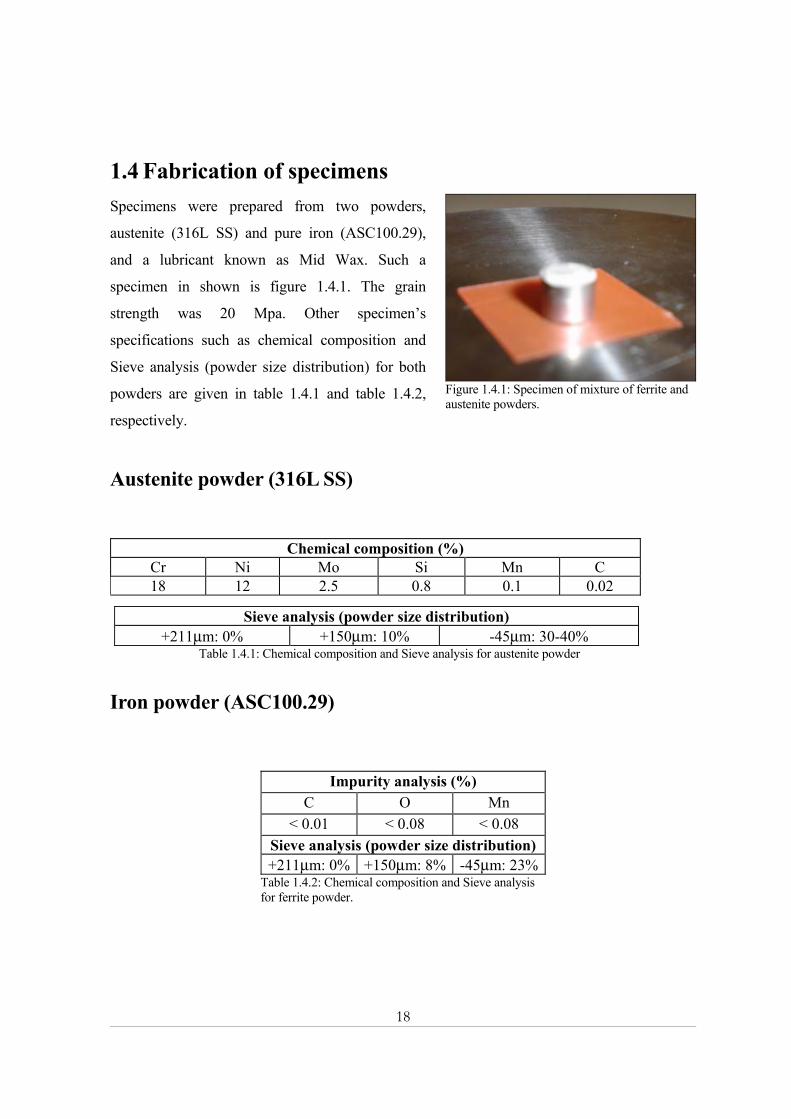
1.4 Fabrication of specimens Specimens were prepared from two powders,

austenite (316L SS) and pure iron (ASC100.29),

and a lubricant known as Mid Wax. Such a

specimen in shown is figure 1.4.1. The grain

strength was 20 Mpa. Other specimen’s

specifications such as chemical composition and

Sieve analysis (powder size distribution) for both

powders are given in table 1.4.1 and table 1.4.2,

respectively.

Austenite powder (316L SS)

Chemical composition (%) Cr Ni Mo Si Mn C 18 12 2.5 0.8 0.1 0.02

Sieve analysis (powder size distribution) +211µm: 0% +150µm: 10% -45µm: 30-40%

Table 1.4.1: Chemical composition and Sieve analysis for austenite powder

Iron powder (ASC100.29)

Impurity analysis (%) C O Mn

< 0.01 < 0.08 < 0.08 Sieve analysis (powder size distribution) +211µm: 0% +150µm: 8% -45µm: 23%

Table 1.4.2: Chemical composition and Sieve analysis for ferrite powder.

Figure 1.4.1: Specimen of mixture of ferrite and austenite powders.

19

Chapter Two Experimental techniques

2.1 X-Ray powder Diffraction (XRD) Crystal structures are studied through the diffraction of photons, neutrons, and electrons. The

diffraction depends on the crystal structure and on the wavelength of incident radiation. So from

a diffraction pattern many structural features can be obtained [5].

X-Ray powder Diffraction (XRD) has a number of advantages over other diffraction methods.

Some of them are listed below.

• Non-destructive analysis.

• Minimal or no sample preparation requirements.

• Ambient conditions.

• Quantitative measurement of phase contents, texture and other structural parameters

such as average grain size, strain and crystal defects.

XRD principle W. L. Bragg presented a very simple explanation of the diffracted beams from a crystal.

The incident X-ray beam gets scattered at all the scattering centers, which lie on the lattice

planes of specimen. The angle between the incident X-ray beam and the lattice planes of the

specimen is called θ. And 2θ is the angle between the incident and scattered X- ray beams. The

2θ of maximum intensity is known as the Bragg angle.

20

The scattered beams at different scattering centers must be scattered coherently, to give

maxima in scattered intensity.

These conditions result in the Bragg equation.

nλ = 2 d sin θ

λ is the wavelength of incident X-rays and d is the distance between two lattice planes of the

specimen.

XRD principle

It is evident from the Bragg equation that if the wavelength is known then the distance between

lattice planes of the sample can be determined, immediately.

Basically, the powder method involves the diffraction of monochromatic X-rays by a powder

specimen. In this connection, “monochromatic” usually means the strong K characteristic

component of the x-ray radiation. “Powder” can mean either an actual, physical powder or any

specimen in polycrystalline form.

This method is thus eminently suited for the metallurgical work, since single crystals are not

always available to the metallurgist. Material such as polycrystalline wire, sheet, rod, etc., may

be examined nondestructively without any special sample preparation.

Powder XRD quantitative phase analysis is the perfect and most powerful technique for multi

component crystalline-mixtures, since each component of the mixture produces its

characteristic pattern independent of the other [5].

Incident X-rays Scattering center

Lattice planes

Scattered X-rays

21

Diffraction Methods Diffraction can occur whenever the Bragg law is satisfied. The Bragg equation puts very

stringent conditions on wavelength and theta. Some way of satisfying the Bragg law must be

devised, as any arbitrary setting of a sample in a beam of monochromatic X- ray will not in

general produce diffraction beams. It can be done by continuously varying either wavelength or

theta. There are three different diffraction methods to vary these two parameters [5].

Diffraction Method Wavelength Theta

Laue method

Variable

Fixed

Rotating -crystal method

Fixed

Variable (in part)

Powder method

Fixed

Variable Table 2.1: Different diffraction methods

22

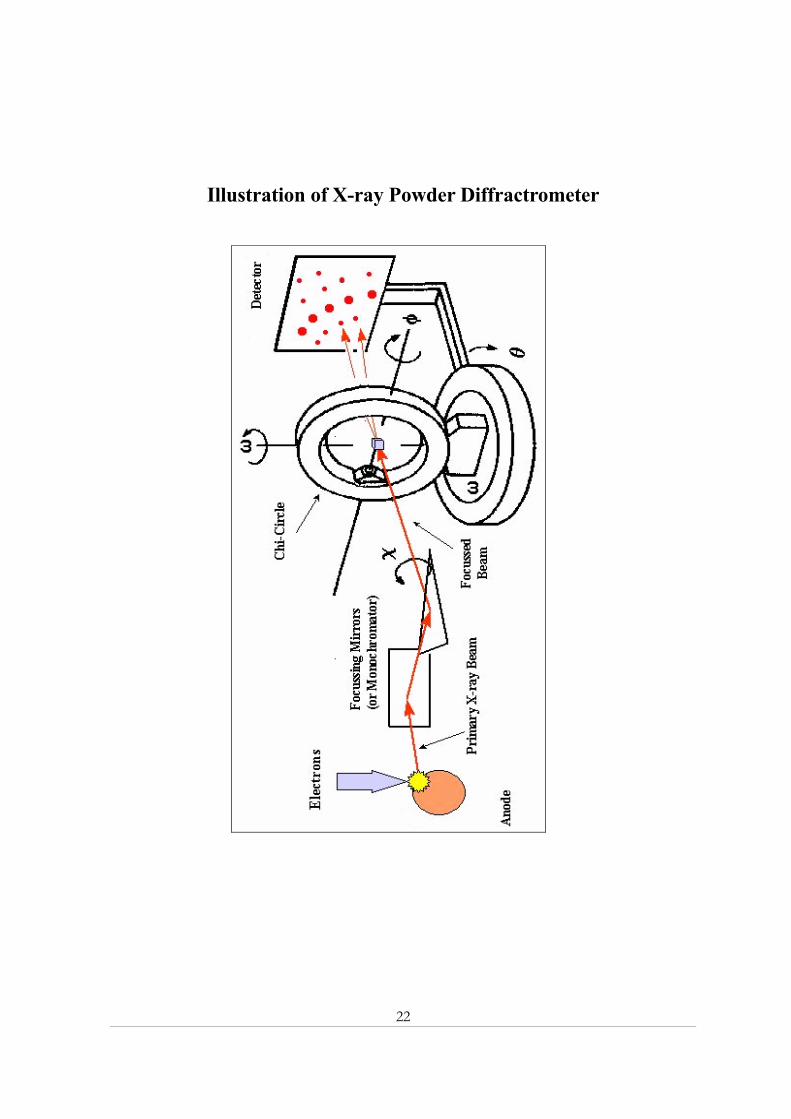
Illustration of X-ray Powder Diffractrometer

23

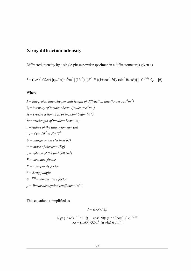
X ray diffraction intensity Diffracted intensity by a single-phase powder specimen in a diffractometer is given as

I = (IoAλ3 /32πr) [(µo/4π) ℮4/m 2] (1/υ 2) [|F|2 P {(1+ cos2 2θ)/ (sin 2 θcosθ)}] ℮ - (2M) /2µ [6] Where I = integrated intensity per unit length of diffraction line (joules sec-1m-1)

Io = intensity of incident beam (joules sec-1m-1)

A = cross-section area of incident beam (m-2)

λ= wavelength of incident beam (m)

r = radius of the diffractometer (m)

µo = 4π * 10-7 m Kg C-2

℮ = charge on an electron (C)

m = mass of electron (Kg)

υ = volume of the unit cell (m3)

F = structure factor

P = multiplicity factor

θ = Bragg angle

℮ - (2M) = temperature factor

µ = linear absorption coefficient (m-1)

This equation is simplified as

I = K2 R2 / 2µ

R2= (1/ υ 2) [|F|2 P {(1+ cos2 2θ)/ (sin 2 θcosθ)}] ℮ - (2M)

K2 = (IoAλ3 /32πr) [(µo/4π) ℮4/m 2]

24

There are number of factors, which affect the relative intensity of the diffraction lines on a

powder pattern, which are listed below.

1- Polarization-Lorentz factor (1+ cos2 2θ)/sin 2 θcosθ), 2- Structure factor (F), 3- Multiplicity

factor (P),4- Absorption factor (µ),5- Temperature factor (℮ - (2M)).

2.1.1 Quantitative phase analysis by X- ray powder diffraction Quantitative phase analysis by the XRD is based on the fact that the intensity of the diffraction

pattern of a particular phase in a mixture of phases depends on the concentration of that phase in

the mixture.

The particular advantage of this method is that it discloses the presence of a substance as that

substance actually exists in the sample, and not in terms of its constituent chemical elements.

Quantitative phase analysis by the XRD is the perfect method for crystalline mixture analysis,

since each component of the mixture produces its characteristic pattern independently of the

others, making it possible to identify the various components.

Unlike quantitative phase analysis by the XRD, chemical quantitative analysis gives elemental

composition of a material, but usually has great difficulty in distinguishing the chemical identity

of the various phases present [29]. For example, the chemical analysis of carbon steel reveals

only the amount of iron, carbon, etc., which the steel contains, but gives no information

regarding the phases present. Whereas quantitative phase analysis by the XRD gives full

information about the phases present such as ferrite, martensite and austenite

Thus analytical determinations such as quartz in the presence of mineral silicates, mixed alloy

phases of different proportions of the same elements, and the relative amounts of polymorphs in

mixtures are handled routinely by diffraction, but are difficult or impossible by chemical

methods [29].

Other than this, quantitative phase analysis by the XRD can effortlessly distinguish between

different allotropic modifications of the same sample.

25

Because of its abilities, this method has been widely used for analysis of materials as alloys,

corrosion products, industrial dusts, etc [6].

Quantitative Methods Numerous methods have been developed to use integrated intensities for quantitative analysis of

the diffraction pattern obtained from a given sample. For example, Internal Standard Method,

External Standard Method, Direct Comparison Method, The absorption-diffraction method,

Method of standard additions etc.

Following is a short account of two of them and the method used in this work, Direct

Comparison Method.

The Internal Standard Method is the procedure in which, a known quantity of a reference

powder is added to the unknown. Any number of constituents in a mixture may be quantified

independently. The mass absorption coefficient of the mixture need not be known in advance.

The Internal Standard Method is applied broadly to any mineral or materials systems for which

the chemistry is unknown. This may be applied to solid systems, such as alloys, plasma sprayed

coatings, or oxide layers [6].

The External Standard Method allows the quantification of one or more components in a

system, which may contain an amorphous fraction. The mass absorption coefficient must,

however, be known in advance, requiring prior knowledge of the chemistry, as in the case of

plasma spray coatings or alloys [6]

The Direct Comparison Method requires no standards as needed in other methods mentioned

above. This method is of immense metallurgical interest because it can be applied directly to

polycrystalline aggregates. Since its development, it has been used for instance to measure the

amount of retained austenite in hardened steel [6].

For specimens containing only two-phases, austenite (α) and ferrite (γ), the governing equation

for this method is given as

Iγ/ Iα = Rγ Cγ / Rα C α

26

Iγ and Iα are the measured diffracted integrated intensities from austenite (α) and ferrite (γ)

phase, respectively. These integrated intensities could be either from all diffracted peaks or

only one, with highest number of counts, from each phase.

R= (1/ υ 2) [|F|2 P {(1+ cos2 2θ)/ (sin 2 θcosθ)}] ℮ - (2M)

R values are known as theoretical diffracted intensities. It consists of all factors, which can

affect the diffracted intensities, as mentioned earlier.

K2 = (IoAλ3 /32πr) [(µo/4π)2 ℮4/m 2]

Cγ, Cα are the concentrations of the phases, austenite (α) and ferrite (γ), respectively

The general and simplified equation for integrated intensity is given as

I = K2 R / 2µ

The phase quantification by direct comparison requires two such equations, one for each phase.

Iγ = Rγ K2Cγ / 2µ

Iα = Rα K2Cα / 2µ

The value of the Cγ / C γ can therefore is obtained from a ratio of measured intensities, Iγ/ Iα and

a calculation of Rγ / Rα. Once Cγ / Cα is found, the value of (say) Cγ is then found from the

relation.

Cγ + C γ = 1

In choosing diffraction lines to measure, one must be sure to avoid overlapping or closely

adjacent lines from different phases. This method can easily be extended to any number of

diffraction lines (or peaks) from each phase present in the specimen.

27

Theoretically calculated intensities, R values, for austenite (α) and ferrite (γ) phase, can be

obtained from scientific literature such as published by ASTM [21]. Values of theoretical

intensities can also be calculated using a computer based program called Lazy Pulverix [31].

Experimental limitations It may be difficult to obtain an accurate value for diffracted intensities. The intensities of the

diffraction peaks are subject to a variety of errors and these errors fall roughly into three

categories:

A) Structure-dependent: that is a function of atomic size and atomic arrangement, plus some

dependence on the scattering angle and temperature.

B) Instrument-dependent: that is a function of diffractometer conditions, source power, slit

widths, detector efficiency, etc.

C) Specimen-dependent: that is a function of phase composition, specimen absorption, particle

size, distribution and orientation.

For a given phase, or selection of phases, all structure dependent terms are fixed, and in this

instance have no influence on the validity of the quantitative procedure. Provided that the

diffractometer terms are constant, this effect can also be ignored.

Specimens used in this work, consist of small crystallites that are randomly oriented as required

for powder XRD.

Practical Difficulties As stated above, the possible reasons for intensity variation in quantitative phase analysis by the

XRD can be divided in to three categories, structure-dependent, instrument-dependent and

specimen-dependent.

In this section some of most important specimen-dependent factors are studied in detail, namely

preferred orientation, microabsorption and extinction.

Preferred Orientation

The basic intensity equation is derived for a specimen where constituent crystals are randomly

oriented. In case of a solid polycrystalline specimen, it is impossible to have full control over its

28

distribution of orientation, but one should be aware of the possibility of the error due to

preferred orientation (texture).

For example, in the determining of austenite in steel we can have a quick check of texture. If the

measured intensities of the various lines of a particular phase are not in the same ratio as their R

values then texture exists.

Microabsorption

If the mass absorption coefficient of one phase, in a mixture, is much larger than of the other or

if the particle size of one phase is much larger then other, the total intensity of that phase will be

much less than calculated, since the effect of micro absorption in that phase in not included in

the basic intensity equation.

Evidently, the micro absorption effect is negligible when mass absorption coefficients and

particle sizes of all constituent phases are the same or their particle size is very small.

Extinction

The decrease in the integrated intensity of the diffracted beam as the crystal becomes nearly

perfect is called extinction. The basic intensity equation is derived for the ideally imperfect

crystal, one in which extinction is absent.

Micro absorption and Extinction, if present, can seriously decrease the accuracy of the direct

comparison method, because it is an absolute method.

The both effects are negligible in the case of hardened steel. Extinction is also absent because of

the very nature of hardened steel [5].

2.1.2 Statistical Error It should always be kept in mind that the statistical error determines the quality of the results

Precision in establishing the profile, and hence the position, of a diffraction line is based mainly

on the statistical error in number of counts.

29

X-ray photons generated by the anode of an X- ray tube are emitted in a random manner both

with respect to direction and time. Hence, if the intensity of the narrow beam is measured for a

very short time, it will be found to fluctuate in a statistical manner above and below a certain

mean level. This deviation from the mean intensity reduces with increase in measuring time and

at sufficiently long time intervals become imperceptible [29]. The amount of phase under

consideration also affects the variation in intensity.

These facts have a significant bearing upon the measurement of diffraction intensities. Hence it

is important to bear in mind continuously the magnitude of statistical error. The probable error

is proportional to 1/√N, where N is the number of counts [5].

Statistical errors for each measurement were calculated and are presented in Appendix 2.

2.1.2 Full-Pattern phase quantification The full-pattern method of quantitative analysis has several significant advantages over the tow

lines method, where the strongest peaks, one from each of phase of the multiphase sample are

employed. Because in full-pattern quantitative phase analysis by the XRD the problems in

obtaining reproducible intensities and in dealing with overlapped profiles are eliminated.

Ambiguities in determining background position during intensity measurements are also largely

eliminated. In addition, some of the more troublesome effects such as preferred orientation and

extinction are minimized [25].

30

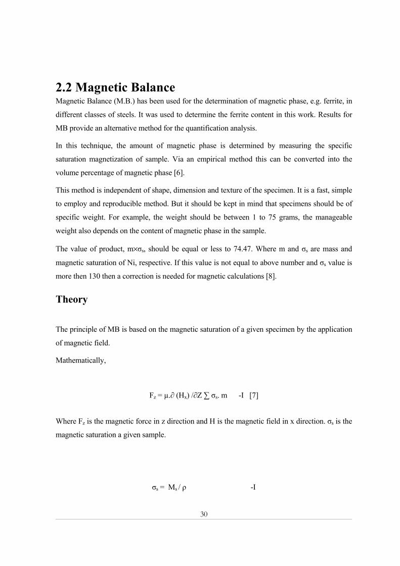
2.2 Magnetic Balance Magnetic Balance (M.B.) has been used for the determination of magnetic phase, e.g. ferrite, in

different classes of steels. It was used to determine the ferrite content in this work. Results for

MB provide an alternative method for the quantification analysis.

In this technique, the amount of magnetic phase is determined by measuring the specific

saturation magnetization of sample. Via an empirical method this can be converted into the

volume percentage of magnetic phase [6].

This method is independent of shape, dimension and texture of the specimen. It is a fast, simple

to employ and reproducible method. But it should be kept in mind that specimens should be of

specific weight. For example, the weight should be between 1 to 75 grams, the manageable

weight also depends on the content of magnetic phase in the sample.

The value of product, m×σs, should be equal or less to 74.47. Where m and σs are mass and

magnetic saturation of Ni, respective. If this value is not equal to above number and σs value is

more then 130 then a correction is needed for magnetic calculations [8].

Theory The principle of MB is based on the magnetic saturation of a given specimen by the application

of magnetic field.

Mathematically,

Fz = µ.∂ (Hx) /∂Z ∑ σs. m -I [7]

Where Fz is the magnetic force in z direction and H is the magnetic field in x direction. σs is the

magnetic saturation a given sample.

σs = Ms / ρ -I

31

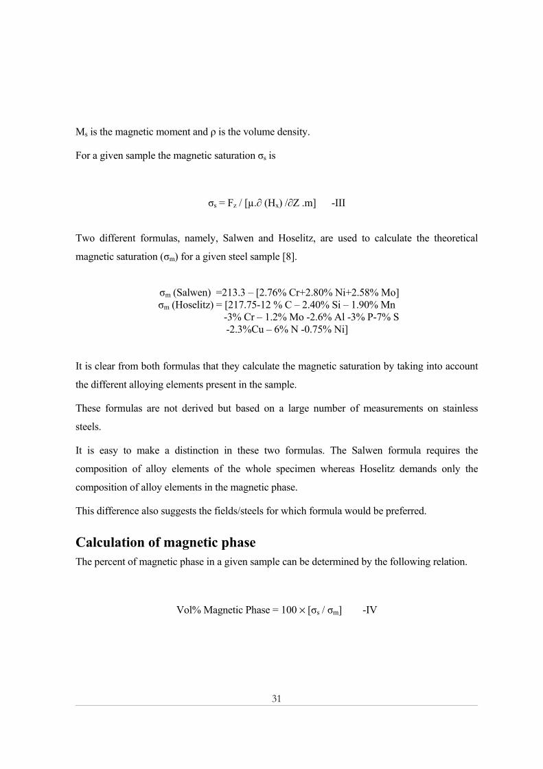
Ms is the magnetic moment and ρ is the volume density.

For a given sample the magnetic saturation σs is

σs = Fz / [µ.∂ (Hx) /∂Z .m] -III

Two different formulas, namely, Salwen and Hoselitz, are used to calculate the theoretical

magnetic saturation (σm) for a given steel sample [8].

σm (Salwen) =213.3 – [2.76% Cr+2.80% Ni+2.58% Mo] σm (Hoselitz) = [217.75-12 % C – 2.40% Si – 1.90% Mn

-3% Cr – 1.2% Mo -2.6% Al -3% P-7% S -2.3%Cu – 6% N -0.75% Ni]

It is clear from both formulas that they calculate the magnetic saturation by taking into account

the different alloying elements present in the sample.

These formulas are not derived but based on a large number of measurements on stainless

steels.

It is easy to make a distinction in these two formulas. The Salwen formula requires the

composition of alloy elements of the whole specimen whereas Hoselitz demands only the

composition of alloy elements in the magnetic phase.

This difference also suggests the fields/steels for which formula would be preferred.

Calculation of magnetic phase The percent of magnetic phase in a given sample can be determined by the following relation.

Vol% Magnetic Phase = 100 × [σs / σm] -IV

32

Experimentally, the magnetic saturation, known as σs, of a given specimen is obtained by the

application of magnetic field and using following relations.

σs = K × α / m

K = constant, α = difference in the micrometer readings in load and unload condition (mm)

and m = weight of the specimen (grams)

Then the theoretical magnetic saturation, known as σm, of that specimen is calculated either by

Salwen or Hoselitz’s formula. The amount of magnetic phase is determined by the use of

equation IV [8].

Vol% Magnetic Phase = 100 × [σs / σm]

Source of error

The accuracy of the magnetic measurement is mainly dependent on the saturation

magnetization of a fully magnetic sample [14]. Imperfections in the magnetic field, variation in

spring modulus and difference in sample weight, can also partly affect the accuracy of the

measurements [15].

33

2.3 Image Analysis Image analysis is a method for study of microstructures, especially in case of images of

materials where the constituents have sharp contrast. In more complex images, however,

significant image processing needs to be performed to extract the desired information.

Depending on resolution requirements, an image can be obtained from light optical microscopy

or such as scanning electron microscopy (SEM) [12].

The basis for image analysis is a digitized image, where each picture element (pixel) represents

a specific grey level. The difference in grey levels is used to determine the phase of interest.

Some applications of image analysis are given below [9].

• Determination of grain size, grain shape, grain boundary.

• Quantitative determination of second-volume fraction.

• Quantitative determination of particle size distributions in powders.

2.3.1 Procedure of image analysis Image acquisition A digital type of detector such as a CCD camera, backscatter electron or secondary electron or

EBSD detector etc. can be used to capture an image from a given specimen. It is mounted on a

microscope, light or electron. If a digital camera is not used then the image needs to be

converted into a digital image so that the computer can read it. Both spatial and frequency

distributions are made digital.

Frequency distribution is known as grey level. The digitizer converts the analog signal from the

camera into a digitized scale of 8 bits (or 2 8= 256 grey levels). This means that white color has

a digitized value of 255 and the black color has the value 0. This gives all grey levels a digitized

value. Any image can be described in terms of a histrogram of its grey levels.

Spatial characterizations of an image can be digitized into an array of rectangular segments

called Pixels. Images can be digitized into 8 bits or 512*512 pixel arrays.

34

However, image digitization into 1024, 2048 and 4096 pixel systems is also possible.

The ability of the computer to manipulate information and the accuracy of the measurement

increase with the number of pixels and fineness of grey levels [29].

The Grey image processing Image analysis is based on the fact that the phase of interest has a different grey level than the

matrix.. The grey image processing helps to produce an image without any defects. It provides

many operations like smoothening and sharpening algorithms, to deal with noise and edge

blurring. These are just some examples of many operations used in grey image processing.

Some times, it is impossible to reach optimal quality of an image.

Thresholding and Binary image processing The thresholding operation creates an image that consists of specific bands of unique grey level.

Boundaries of the phase of interest are also outlined [12].

Based on the grey level range, the image is transformed into a binary black and white image.

During this process information can easily be lost, so utmost care is required.

There are a wide range of operations, which can be used to “clean up” the binary image. These

are briefly discussed here.

Erosion shrinks the objects pixel by pixel and Delineation operator expands the object pixel by

pixel. Open is erosion followed by dilation (eliminate small objects only). Close is dilation

followed by erosion (to connect separated segments). Boolean operators are also possible.

After the accomplishment of thresholding a binary image is ready for desired analysis.

A small difference in grey levels and low pixel resolution can be significant sources of error in

thresholding.Thresholding is not always easy. The most common source of error is finding the

boundary between the regions of interest and the background.

2.3.2 Possible errors • The representative character of the sample.

• Quality of sample preparation.

35

• Operator bias in setting controls [9].

Scanning Electron Microscope

aperture

valve

36

2.3.2 Scanning Electron Microscope

The Scanning Electron Microscope (SEM) is a microscope that uses electrons to form an image.

There are many advantages in using the SEM instead of a light microscope.

The SEM produces images of high lateral resolution, which means that closely spaced features

can be examined at a high magnification. Preparation of the samples is relatively easy since

most SEMs only require the sample to be conductive. The combination of higher magnification,

larger depth of focus, greater resolution, and ease of sample preparation makes the SEM one of

the most heavily used instruments in materials research areas today.

Material examination by SEM can yield the following information:

Morphology The shape and size of the particles making up the object. (SEI, BEI)

Crystallographic Information How the atoms are arranged in the object. (EBSD)

Composition The elements and compounds that the object is composed of and the relative amounts of them

(EDX or WDX).

2.3.2.1 Operations Electron source The electron beam comes from a filament, made of one of various types of materials. The most

common is the Tungsten hairpin gun. This filament is a loop of tungsten, which functions as the

cathode. A voltage is applied to the loop, causing it to heat up. The anode, which is positive

with respect to the filament, forms powerful attractive forces for electrons. This causes electrons

to accelerate toward the anode. Some accelerate right by the anode and on down the column, to

the sample. However, a filament of LaB6 provides a stronger electron source than Tungsten.

Another example of electron source is field emission gun.

37

Electromagnetic lens and Aperture A thin (<100 micrometer thick) disk or strip of metal (usually Pt) with a small (2-100

micrometers) circular through-hole is used as aperture in SEM. Its basic purpose is to restrict

the electron beam diameter and filter out unwanted scattered electrons before image formation.

The electro-magnetic lens is capable of projecting a precise circular magnetic field in a

specified region. This acts like an optical lens, having the same attributes (focal length, angle of

divergence) and errors (spherical aberration, chromatic aberration). They are used to focus and

steer electrons in an Electron Microscope.

Vacuum in SEM There are many reasons to use vacuum in the SEM. If the sample is in a gas filled environment,

an electron beam cannot be generated or maintained because of a high instability in the beam.

Gases could react with the electron source causing it to burn out, or cause electrons in the beam

to ionize, which produces random discharges and leads to instability in the beam.

The transmission of the electron beam would also be hindered by the presence of other

molecules. Those other molecules, which could come from the sample or the microscope itself,

could form compounds and condense on the sample. This would lower the contrast and obscure

details in the image. However, the so-called variable vacuum and low vacuum SEM have been

developed for the applications such as biology or corrosion studies.

Specimen Preparation As SEM uses electrons to produce an image, most conventional SEMs require that the samples

be electrically conductive. In order to view non-conductive samples such as ceramics or

plastics, samples should be covered with a thin layer of a conductive material. A small device

called a sputter coater may be used for this purpose.

Samples should be polished and etched (if needed) for phase analysis.

How SEM works SEM functions exactly as its optical counterpart except that it uses a focused beam of electrons

instead of light to "image" the specimen and gain information as to its structure and

38

composition.

The basic steps involved in SEM are given in the following text.

A stream of electrons is formed and accelerated toward the specimen using a positive electrical

potential. This stream is confined and focused using metal apertures and magnetic lenses into a

thin, focused, monochromatic beam. This beam is focused onto the sample using a magnetic

lens. Interactions occur inside the irradiated sample, affecting the electron beam.

2.3.2.2 Specimen / electron beam interaction In case of bulk samples, Backscattered Electrons, Secondary Electrons, Auger Electrons and X-

rays from the specimen can be detected

In SEM, usually, BE, SE and X-ray signals are detected.

39

2.3.3 Electron backscatter diffraction Electron backscatter diffraction (EBSD) is an established technique for analyzing the

crystallographic microstructure of single and multiphase materials.

The crystallographic information extracted from the EBSD pattern (Kikuchi pattern) is then

compared with the crystallographic information (for example, phase identification) from

candidate phases, and a best-fit match is determined. Fully automated indexing of EBSD

patterns is achieved by introducing Hough transformation.

Many computer based programs for EBSD pattern’s indexing are commercially available.

Problems may arise when two phases have similar crystal structures or when high residual

stress exists in the sample and then the task for identification may become difficult.

There were two important reasons for using this mode of SEM.

A) Etching (Specimen preparation), as required in other modes of SEM, is not considered

suitable for powder specimens at all. In addition, it creates uncertainly about phase boundaries.

In that case it is difficult to assign boundary to one phase.

B) Phase contrast; backscatter electron imaging (BEI) and energy dispersive X-rays (EDX)

modes of SEM were first employed for imaging. But neither of them could give enough

contrast as required by automatic image analysis.

BE and EDX images are given in appendix 3.

Principle Electron backscatter diffraction is based on Bragg diffraction law.

nλ = 2 d sin θ

λ is the wavelength of electrons, θ is angle of incident beam with respect to specimen and d is

the distance between two lattice planes of the specimen

40

Backscattered electron diffraction from a specimen gives

an EBSD pattern. The EBSD pattern consists of a number

of parallel lines, which are in pairs. The line pair consists of

a bright line (its intensity is higher than background) and a

dark line (its intensity is lower than background). Figure

2.3.2 illustrates the formation of EBSD pattern and its

geometry.

The distance between these two lines w, can be estimated

from the Bragg equation

w ≈ 2 θ ≈ (1/ λ) / d

EBSD gives rise to third dimension to SEM, which is the crystal structure information in

addition to morphology (SEI, BEI) and chemistry (EDX or WDX).

Fig.2.3.2 The formation of an EBSD pattern and its geometry. a. Point source of inelastic scattered electron; b. The geometric construction of Kikuchi pattern; c. The cross-section of intensity of Kikuchi pattern

Figure2.3.1. A typical EDSD pattern

41

Automated indexing From the experimental Kikuchi pattern in EBSD in Fig.2.3.3a the detected bands in the EBSD

pattern are obtained after background subtraction as shown in Fig.2.3.3b. Then so-called Hough

transformation is carried out so that lines in the Kikuchi pattern can be described in Polar

coordinates. A Kikuchi band represents a given atomic plane and the atomic plane can be

described using its normal vector. Thus, what actually Hough transformation does is

transformation of Cartesian coordinates of this vector into Polar coordinates,

ρ =x cos θ +y sin θ,

as shown in Fig. 2.3.3c. Then the Hough space for the given pattern is obtained as shown in Fig.

2.3.3d. If the Hough space is calculated from a known crystal structure and comparison is made

with the experimental one after considering the experimental error, solution to the pattern can

be obtained as shown in Fig. 2.3.3e.

Figures 2.3.4a and 2.3.4b show an indexed EBSD pattern and orientation of an individual grain.

Fig.2.3.3a. A typical EBSD pattern. Fig.2.2.3b.Detected bands in EBSD pattern shown

in Fig.2.3.3a.

AA B D

C E G

I

K M

42

Fig. 2.3.3c. Hough transformation ρ =xcosθ +ysinθ: from Cartesian coordinates to Polar coordinates

Fig. 2.33d. Hough Space transformed from pattern Fig. 2.3.3e. Detected peaks in Hough space.

Fig. 2.3.4a. The indexed EBSD pattern. Fig. 2.3.4b. Point analysis showing the orientation

of individual grains.

43

EBSD Mapping In EBSD mapping the electron beam scans the desired area on the sample gradually. At every

step the EBSD patterns are captured and evaluated. In other words, at each step the phase is

identified by EBSD, as the EBSD or Kikuchi patterns show clear relationship to the crystal

structure in accordance with Bragg diffraction conditions [20]. Every significant change

correlates with the transition to another phase.

By assigning a particular grey level to a phase of interest, area (phase fraction) occupied by that

phase can be estimated.

Instrumentation

Fig.2.3.5 The instrumentation of EBSD in SEM

The main components of the ESBD system are a phosphor screen for the detection of the ESBD

system - patterns, a highly sensitive low light camera for capturing images, an image processing

system, a computer (PC) for data evolution and the SEM-control system that allows the selected

area to be scanned [1].

Sample preparation Because diffracted electrons escape from within only a few tens of nanometers of the specimen

surface, specimen preparation for EBSD is critical to achieve good results.

44

If material near the surface is deformed, or has any surface contaminant, oxide or reaction

product layers present, then EBSD pattern formation may be suppressed.

Specimens should be flat enough to give diffraction, as they are placed at 70 degrees to incident

beam and which make a very small angle with the surface of specimen

2.3.3.1 Applications Typical applications of EBSD are the determination of crystallographic orientation

(misorientation, preferable orientation, etc), grain size, and phase discrimination.

Although EBSD could find very many applications in our daily work the interpretation of the

results requires a deep knowledge of both material and crystallography.

2.3.3.2 Comparison with X-ray powder diffraction (XRD) EBSD is a surface analysis method whereas XRD is a bulk method. EBSD has much better

spatial resolution than XRD but XRD has higher orientation accuracy. The analysis for

crystallographic orientation using EBSD can be related to individual grain whereas XRD is a

statistical method.

45

Chapter Three Experimental

3.1 X-ray Powder Diffraction

A BRUKER ADVANCED D8 diffractrometer equipped with chromium Kα1 radiation

(λ = 2.2897 Å) was used for X-ray diffraction analysis. The following table contains

information about instrumental specifications.

Instrumental specifications 2theta circle Chi circle Phi circle X translation Y translation Z translation Max. Sample Weight Max. Sample height Detector

-5o to 165o -5o to 91.5o -360o to 360o -75 to 75mm -75 to 75mm -1 to 11.5mm 3 Kg 40 mm Sold state detector

Table 3.1.1: Instrumental specifications There were two reasons for using chromium X- ray radiation.

1- Chromium radiation produces a minimum of X- ray fluorescence of Iron.

2- Chromium radiation gives better resolution. [24]

XRD analysis was based on two different kinds of 2 theta ranges.

1. Two peaks, one peak from each phase (Two theta range was from 64.5 to 71 degrees).

2. The whole pattern, three peaks from each phase (Two theta range was from 64.5 to

164.5 degrees).

Samples were analyzed for different measurement time intervals, 7, 14, 24 and 48 hours.

46

Based on preliminary measurements a time interval of 48 hours observed as appropriate with

respect to statistical error.

The following table is showing specifications of phase composition in different specimens.

Specimen 1-a 1-b 2-a 2-b 3-a 3-b 4-a 4-b 5-a 5-b Ferrite 2% 2% 5% 5% 10% 10% 20% 20% 50% 50% Austenite 98% 98% 95% 95% 90% 90% 80% 80% 50% 50%

Table 3.1.2 : Phase composition of samples

3.1.1 Topas Topas is a graphics based profile analysis program built around a general non-linear least

squares fitting system, specifically designed for powder diffraction line profile analysis. It

integrates various types of X-ray analysis by supporting all profile fitting methods currently

employed in powder diffractometry:

• Single line fitting up to the whole pattern fitting

• Whole powder pattern decomposition (Pawley and LeBail method)

• Rietveld structure refinement and quantitative Rietveld analysis

• Ab-initio structure solution from powder data in direct space

Topas is sub divided into two categories, namely, Topas R and Topas P.

Topas-R Topas R is designed for the profile analysis of X-ray powder diffraction data with reference to a

crystal structure model.

This includes Rietveld structure refinement, quantitative Rietveld analysis and Ab-initio

structure solution from powder data in direct space.

Applications of Topas R include crystal structure solution and refinement, standard-less

microstructure analysis and quantitative analysis.

Topas-R gives observed and calculated profiles, their difference and percentage volume phase

fraction.

47

Topas Eva

Topas R Topas P Volume phase fraction

Integrated intensities

Integrated intensities

Topas 3.1.3: Software used to obtain integrated intensities using XRD.

Above table shows the information, which can be obtained from Topas R, Topas P, and Eva.

Topas-P Topas R is designed for the profile analysis of X-ray powder diffraction data without reference

to a crystal structure model, but with reference to emission profile.

This includes the Single line fitting up to the whole pattern fitting as well as whole powder

pattern decomposition (Pawley and LeBail method).

Applications of Topas P include the determination of accurate profile parameters (peak

positions, Peak width, peak shape and integrated intensities)

Accurate profile parameters lead to better results in many related application such as phase

quantitative analysis.

Topas-P gives the observed and the calculated profile, their difference, and integrated

intensities.

These integrated intensities are used to calculate percentage phase fractions of austenite and

ferrite with the help of the direct method [22].

Eva Eva gives integrated intensities without reference to crystal structure and emission profile.

Like Topas-P, these integrated intensities used to calculate percentage phase fractions of

austenite and ferrite with the help of direct method.

3.1.2 Direct comparison method The direct method was used to calculate volume fraction from integrated intensities measured

by Topas P and Eva. It is a theoretical method of phase quantification. Following are the main

equations used in this method.

48

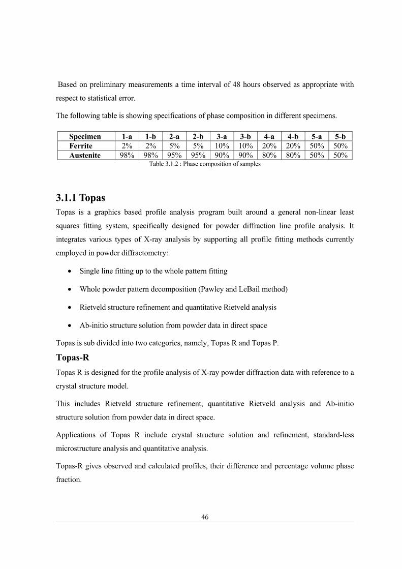
Iγ/ Iα = Rγ Cγ / Rα C α

Cγ +C α = 1

Where Iγ and Iα are integrated intensities of austenite and ferrite phase, respectively, obtained

from Topas P and Eva. Rγ and Rα are known as theoretical intensities and these were calculated

with the help of computer-based software, Lazy Pulverix.

2-theta

Figure 3.1.1Quantitative analysis with Topas R An example of phase quantification by Topas R is given in figure 3.1.1. Observed (Blue),

calculated (Red) profiles, the residual (Grey), and percentage volume fractions are shown.

2-theta

Figure 3.1.2 Quantitative analysis with Topas P.

No. of Counts

Austenite 53 % Ferrite

47 %

Ferrite (Counts) 8 973

No. of Counts

Austenite (Counts) 8541

49

Figure 3.1.2 shows an example of integrated intensities calculation by Topas P. Observed

(Blue), calculated (Red) profiles, the residual (Grey), and integrated intensities are shown.

Figure 3.1.3 Quantitative analysis by Eva Figure 3.1.3 shows an example of integrated intensities calculation by Eva. Observed (Blue)

and integrated intensities are shown.

No.of Counts

Austenite (Counts) 389

Ferrite (Counts) 366

50

3.2 Magnetic balance A direct current of 10A was applied to the magnetic balance, which produced a magnetic field

of 12400 Oe (Oersted1). This magnetic field was sufficient for saturation magnetization to

occur.

First, the magnetic balance was calibrated with respect to a reference sample made of pure

Nickel. After that the measurement was performed by the measuring the deviation in the

position of the specimen holder with and without a specimen, followed by an empty balance

measurement. Finally, a measurement with the reference sample of Nickel was made again.

Both, Salwen and Hoselitz, formulas were used for the calculation of magnetic (ferrite) phase.

σm (Salwen) = 213.3 – [2.76% Cr+2.80% Ni+2.58% Mo]

σm (Hoselitz) = [217.75-12 % C – 2.40% Si – 1.90% Mn

-3% Cr – 1.2% Mo -2.6% Al -3% P-7% S

-2.3%Cu – 6% N -0.75% Ni]

3.3 Electron backscatter diffraction (EBSD)

3.3.1 Specimen preparation

Sample mounting The samples were imbedded in a transparent mounting resin, known as Buehler Transoptic

Powder.

Sample grinding Specimen grinding was done for three minutes under the force of 120N-150 N. It was repeated

for couple of times.

1 1 A/m = 4π×10-3 Oe

51

Sample polishing Polishing was done with 6µm-1 µm diamond suspension, followed by Silica polishing.

MASTERMET was the chemical product used for this purpose. The whole specimen polishing

processing took 20 minutes. Force during the polishing was 120N-150 N.

3.3.2 EBSD phase analysis A LEO 1530, equipped with a hot field emission gun, with a Gemini column was used for

EBSD analysis. The accelerating voltage was 20 KV, the working distance was 10 to 12 mm,

and the aperture size was 60 micrometers, which can give a resolution as high as 50nm.

The prepared sample was placed on the specimen holder in the vacuum chamber of SEM. By

applying voltage to the electron beam and selecting an appropriate magnification, an image of

the sample was obtained.

By placing the electron beam at any spot on the sample, EBSD (Kikuchi) Patterns were

obtained, indexed and investigated.

Channel 5, computer software was used for pattern indexing, image processing and further

evaluation (quantification) for two-phases. It helped to index bands in the EBSD pattern and

checked the results of indexing. This is a critical step in EBSD analysis. Computer software can

miss any band to be indexed or can do indexing without actually having a band. This can affect

the phase analysis. Therefore, a great care is needed for this step.

These kinds of errors were corrected manually. This step not only helps to check the calibration

of the system but also gives quick information about phases present in sample.

After that a suitable area (for example, having low porosity) on the sample and step size were

selected for mapping.

The step size was 5 micrometers and the area was 2mm ×0.5 mm for all samples except for the

sample with 2 Vol% ferrite. The area of 800 ×600 micrometers was selected due to statistical

reasons.

52

Chapter Four Results

4.1 Magnetic Balance (MB) Magnetic balance (MB) can only measure the magnetic phase present in a given sample, which

was ferrite phase in this case. Both, Hoselitz and Salwen formulas were used to calculate Sigma

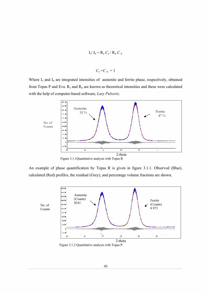
M and then the ferrite volume fraction.

Specimen Hoselitz Salwen Specimen Hoselitz Salwen

1-a 2 4 1-b 2 4 2-a 5 8 2-b 5 9 3-a 10 17 3-b 10 17 4-a 19 31 4-b 20 32 5-a 49 79 5-b 46 75

Table 4.11: Measured values of ferrite volume fraction (Vol%) using Hoselitz and Salwen formula Table 4.11 contains MB results for all specimens. Salwen formula calculated higher ferrite

volume fractions in contrast to Hoselitz formula. Hoselitz formula gave very good accuracy in

both cases than Salwen formula. It is important to note that for both series, a and b, the results

were consistent.

Figure 4.1.1 shows the difference between results obtained from Hoselitz and Salwen formulas

with respect to given ferrite volume fraction. This difference increases with increasing ferrite

volume fraction. Hoselitz formula gave results close to true values for all specimens. Whereas

Salwen formula overestimated ferrite volume fraction for all specimens. The factor of

overestimation increases with increasing volume fraction of ferriteFor samples of series b, the

difference between results obtained from Hoselitz and Salwen formulas with respect to given

values of ferrite volume fraction shown in figure 4.1.2

53

010203040

5060708090

0 10 20 30 40 50 60

Given ferrite volume fraction (Vol%)

Mea

sure

d fe

rrite

vol

ume

frac

tion

(Vol

%)

0

10

20

30

40

50

60

70

80

0 10 20 30 40 50 60

Given ferrite volume fraction (Vol%)

Mea

sure

d fe

rrite

vol

ume

frac

tion

(Vol

%)

Figure 4.1.1: Given values plotted against calculated ferrite phase volume fraction (Vol %), for samples of series a, by Hoselitz and Salwen formulas.

Figure 4.1.2: Given values plotted against calculated ferrite phase volume fraction (Vol %), for samples of series b, by Hoselitz and Salwen formulas.

This difference increases with increasing ferrite volume fraction. Results from Hoselitz formula

showed very good accuracy except for sample with 50 Vol% ferrite. In that case, it

underestimated ferrite volume fraction. Salwen formula overestimated ferrite volume fraction

for all specimens. The factor of overestimation increases with increasing volume fraction of

ferrite.

Sigma S and Sigma M Experimental and theoretical magnetic saturations were plotted with respect to given volume

fraction of ferrite.

0

50

100

150

200

250

300

0 10 20 30 40 50 60

Given ferrite volume fraction (a)

Sigm

a S

& S

igm

a M

0

50

100

150

200

250

300

0 10 20 30 40 50 60

Given ferrite volume fraction(b)

Sigm

a S

& S

igm

a M

Figure 4.1.3: Given ferrite volume fraction (Vol %) plotted against Sigma Sand Sigma M calculated, for samples of series a, by Hoselitz and Salwen formulas

Figure 4.1.4: Given ferrite volume fraction (Vol %) plotted against Sigma S and Sigma M calculated, for samples of series b, by Hoselitz and Salwen formulas.

♦ Hoselitz ■ Salwen ⎯ Given ferrite Vol%

♦ Hoselitz ■ Salwen ⎯ Given ferrite Vol%

• Sigma S (Hoselitz), ♦ Sigma S (Salwen), ▲Sigma M (Hoselitz), × Sigma M (Salwen)

• Sigma S (Hoselitz), ♦ Sigma S (Salwen), ▲ Sigma M (Hoselitz), × Sigma M (Salwen)

54

The variation of measured values of Sigma S and M with respect to given ferrite volume

fraction is shown in above figures. Theoretical magnetic saturations (Sigma M) were observed

constant for each specimen of both series. As expected, their values were different because of

different formulas used for calculation.

Equation IV of section 2.2 shows the direct relationship between percentage magnetic phase

and Sigma S. Figures 4.1.3 and 4.1.4 are mere manifestations of that equation.

Values of Sigma S increase with increasing ferrite volume fraction. The value of Sigma M

depends on the amount of alloy elements and remains constant for one combination of alloy

composition. It is also clear from the above two figures.

Experimental data is given in Appendix 2

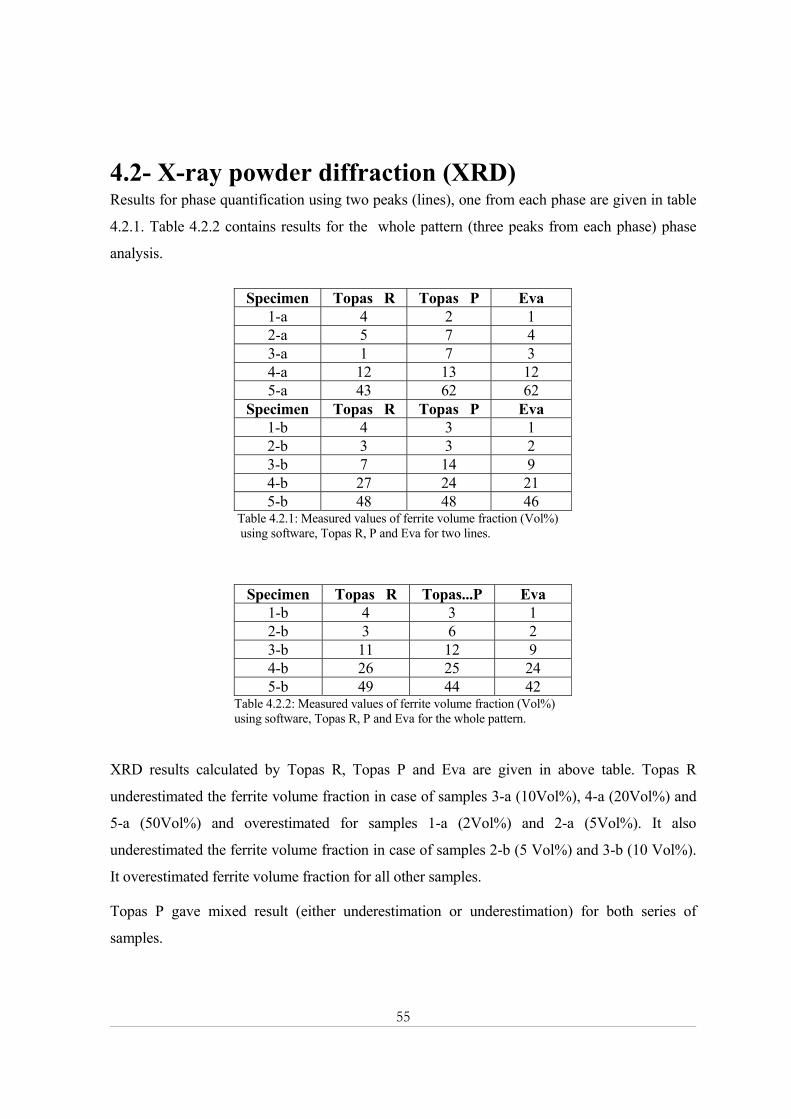
55

4.2- X-ray powder diffraction (XRD) Results for phase quantification using two peaks (lines), one from each phase are given in table

4.2.1. Table 4.2.2 contains results for the whole pattern (three peaks from each phase) phase

analysis.

Specimen Topas R Topas P Eva 1-a 4 2 1 2-a 5 7 4 3-a 1 7 3 4-a 12 13 12 5-a 43 62 62

Specimen Topas R Topas P Eva 1-b 4 3 1 2-b 3 3 2 3-b 7 14 9 4-b 27 24 21 5-b 48 48 46

Table 4.2.1: Measured values of ferrite volume fraction (Vol%) using software, Topas R, P and Eva for two lines.

Specimen Topas R Topas...P Eva 1-b 4 3 1 2-b 3 6 2 3-b 11 12 9 4-b 26 25 24 5-b 49 44 42

Table 4.2.2: Measured values of ferrite volume fraction (Vol%) using software, Topas R, P and Eva for the whole pattern.

XRD results calculated by Topas R, Topas P and Eva are given in above table. Topas R

underestimated the ferrite volume fraction in case of samples 3-a (10Vol%), 4-a (20Vol%) and

5-a (50Vol%) and overestimated for samples 1-a (2Vol%) and 2-a (5Vol%). It also

underestimated the ferrite volume fraction in case of samples 2-b (5 Vol%) and 3-b (10 Vol%).

It overestimated ferrite volume fraction for all other samples.

Topas P gave mixed result (either underestimation or underestimation) for both series of

samples.

56

Eva results showed a clear pattern of underestimation for both series of samples, with exception

of samples 5-a and 4-b.

The whole pattern measurements were also done to determine the existence of preferred

orientation, if any. Results are given in table 4.2.2. Topas R gave the same pattern of over and

underestimation of ferrite volume fractions as in the case of two lines analysis, with one

exception of sample 3-b.

Topas P also gave the same pattern of over and underestimation of ferrite volume fractions as in

case of two lines analysis, with one exception of sample 2-b.

Eva gave consistent results for sample 1-b, 2-b and 3-b. For samples 4-b and 5-b, it gave the

same pattern of over and underestimation but with a larger factor.

0

10

20

30

40

50

60

70

0 10 20 30 40 50 60Given ferrite volume fraction (Vol%)

Mea

sure

d fe

rrite

vol

ume

fract

ion

(Vol

%)

0

10

20

30

40

50

60

0 10 20 30 40 50 60

Given ferrite volume fraction (Vol%)

Mea

sure

d

ferr

ite v

olum

e fr

actio

n (V

ol%

)

Figure 4.2.1: Given values plotted against measured ferrite volume fraction (Vol%), for samples of series a, by Topas R, P and Eva for two lines phase analysis

Figure 4.2.2: Given values plotted against measured ferrite volume fraction (Vol %), for samples of series b, by Topas R, P and Eva for two lines phase analysis.

Variation of XRD results for samples of series a, calculated using Topas R, Topas P and Eva,

with respect to given ferrite volume fraction in figure 4.2.1. The difference between these

results is more significant for sample 5-a than for any other sample. Results were very close to

each other for samples 1-a, 2-a and 4-a. Results were more accurate for samples 1-a and 2-a

than for any other sample.

In figure4.2.2 XRD results are plotted against given ferrite volume fraction, for samples of

series b. In case of 2-b and 5-b, results were found more close to each other than for any other

sample. All, Topas R, Topas P and Eva, underestimated ferrite volume fractions for these two

♦ Topas R ■ Topas P ▲ Eva ⎯ Given ferrite Vol%

♦Topas R ■ Topas P ▲ Eva ⎯ Given ferrite Vol%

57

samples. For other samples, mixed results of underestimations or overestimations were

observed.

Variation in XRD results for sample of

series b (the whole pattern measurements),

calculated using Topas R, Topas P and

Eva; with respect to given ferrite volume

fraction is shown in the figure 4.2.3.

Comparison of results from two lines and

the whole pattern analysis discloses the

following information.

Generally, same pattern of over or

underestimation of ferrite volume fractions was observed as in case of two line analysis. It is

interesting to note that the scatter, in results, was less for sample 1-b, 3-b and 4-b. But result

were more scattered for samples 2-b and 5-b.

4.2.1 Effect of α2 Stripping The α2 stripping chromium radiation was done with the help of Eva and then analyzed with

Topas and Eva. Table 4.2.3 shows the XRD results after eliminating the effect of α2 stripping.

Topas R underestimated the ferrite volume fraction for samples of both series, a and b, with two

exceptions. Topas P gave a mixed pattern of results for samples of both series, a and b. Eva

looked most consistent with only one exception.

Topas R underestimated the ferrite volume fraction in case of samples 1-a, 2-a, 3-a and 5-a. It

overestimated for sample 4-a.

Topas P overestimated ferrite volume fractions for samples 1-a, 2-a and 5-a.It underestimated

sample 3-a. Eva underestimation ferrite volume fractions for all samples but 5-a.

Topas R gave the same pattern of over and underestimation of ferrite volume fractions as in the

case of XRD analysis without stripping, with one exception of sample 3-b. Topas P

overestimated ferrite volume fraction for samples 1-b, 3-b and 4-b. It underestimated ferrite

volume fractions in case of samples 2-b and 5-b.

0

10

20

30

40

50

60

0 10 20 30 40 50 60

Given ferrite volume fraction (Vol%)

Mea

sure

d

ferr

ite v

olum

e fr

actio

n (V

ol%

)

Figure 4.2.3: Given values plotted against measured ferrite volume fraction (Vol%), for samples of series b, by Topas R, P and Eva for the whole pattern phase analysis.

♦ Topas R ■ Topas P ▲ Eva ⎯ Given ferrite Vol%

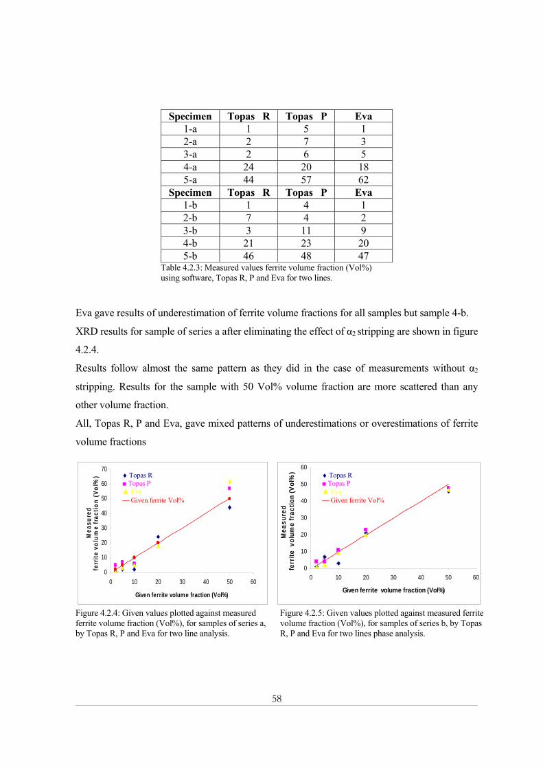
58

Specimen Topas R Topas P Eva

1-a 1 5 1 2-a 2 7 3 3-a 2 6 5 4-a 24 20 18 5-a 44 57 62

Specimen Topas R Topas P Eva 1-b 1 4 1 2-b 7 4 2 3-b 3 11 9 4-b 21 23 20 5-b 46 48 47

Table 4.2.3: Measured values ferrite volume fraction (Vol%) using software, Topas R, P and Eva for two lines.

Eva gave results of underestimation of ferrite volume fractions for all samples but sample 4-b.

XRD results for sample of series a after eliminating the effect of α2 stripping are shown in figure

4.2.4.

Results follow almost the same pattern as they did in the case of measurements without α2

stripping. Results for the sample with 50 Vol% volume fraction are more scattered than any

other volume fraction.

All, Topas R, P and Eva, gave mixed patterns of underestimations or overestimations of ferrite

volume fractions

0

10

20

30

40

50

60

70

0 10 20 30 40 50 60

Given ferrite volume fraction (Vol%)

Mea

sure

d

ferr

ite v

olum

e fr

actio

n (V

ol%

)

0

10

20

30

40

50

60

0 10 20 30 40 50 60

Given ferrite volume fraction (Vol%)

Mea

sure

d fe

rrite

vol

ume

frac

tion

(Vol

%)

Figure 4.2.4: Given values plotted against measured ferrite volume fraction (Vol%), for samples of series a, by Topas R, P and Eva for two line analysis.

Figure 4.2.5: Given values plotted against measured ferrite volume fraction (Vol%), for samples of series b, by Topas R, P and Eva for two lines phase analysis.

♦ Topas R ■ Topas P ▲ Eva ⎯ Given ferrite Vol%

♦ Topas R ■ Topas P ▲ Eva ⎯ Given ferrite Vol%

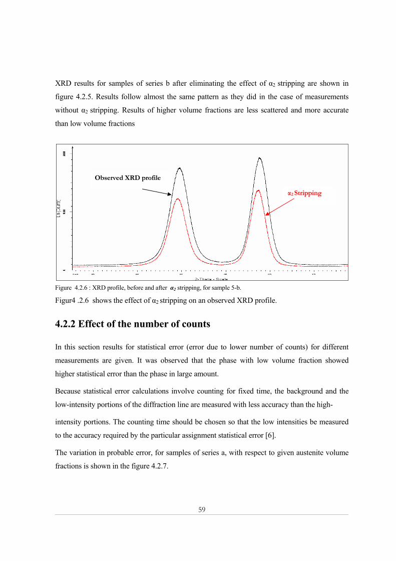
59

XRD results for samples of series b after eliminating the effect of α2 stripping are shown in

figure 4.2.5. Results follow almost the same pattern as they did in the case of measurements

without α2 stripping. Results of higher volume fractions are less scattered and more accurate

than low volume fractions

Figur4 .2.6 shows the effect of α2 stripping on an observed XRD profile.

4.2.2 Effect of the number of counts In this section results for statistical error (error due to lower number of counts) for different

measurements are given. It was observed that the phase with low volume fraction showed

higher statistical error than the phase in large amount.

Because statistical error calculations involve counting for fixed time, the background and the

low-intensity portions of the diffraction line are measured with less accuracy than the high-

intensity portions. The counting time should be chosen so that the low intensities be measured

to the accuracy required by the particular assignment statistical error [6].

The variation in probable error, for samples of series a, with respect to given austenite volume

fractions is shown in the figure 4.2.7.

Figure 4.2.6 : XRD profile, before and after α2 stripping, for sample 5-b.

Observed XRD profile

α2 Stripping

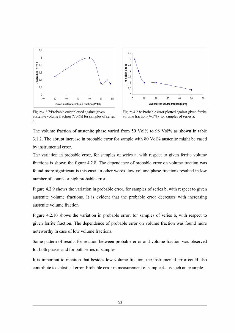
60

0

0,2

0,4

0,6

0,8

1

1,2

40 50 60 70 80 90 100

Given austenite volume fraction (Vol%)

Prob

able

err

or

0

0,5

1

1,5

2

2,5

3

3,5

0 10 20 30 40 50 60

Given ferrite volume fraction (Vol%)

Prob

able

err

or

Figure4.2.7:Probable error plotted against given austenite volume fraction (Vol%) for samples of series a.

Figure 4.2.8: Probable error plotted against given ferrite volume fraction (Vol%) for samples of series a.

The volume fraction of austenite phase varied from 50 Vol% to 98 Vol% as shown in table

3.1.2. The abrupt increase in probable error for sample with 80 Vol% austenite might be cased

by instrumental error.

The variation in probable error, for samples of series a, with respect to given ferrite volume

fractions is shown the figure 4.2.8. The dependence of probable error on volume fraction was

found more significant is this case. In other words, low volume phase fractions resulted in low

number of counts or high probable error.

Figure 4.2.9 shows the variation in probable error, for samples of series b, with respect to given

austenite volume fractions. It is evident that the probable error decreases with increasing

austenite volume fraction

Figure 4.2.10 shows the variation in probable error, for samples of series b, with respect to

given ferrite fraction. The dependence of probable error on volume fraction was found more

noteworthy in case of low volume fractions.

Same pattern of results for relation between probable error and volume fraction was observed

for both phases and for both series of samples.

It is important to mention that besides low volume fraction, the instrumental error could also

contribute to statistical error. Probable error in measurement of sample 4-a is such an example.

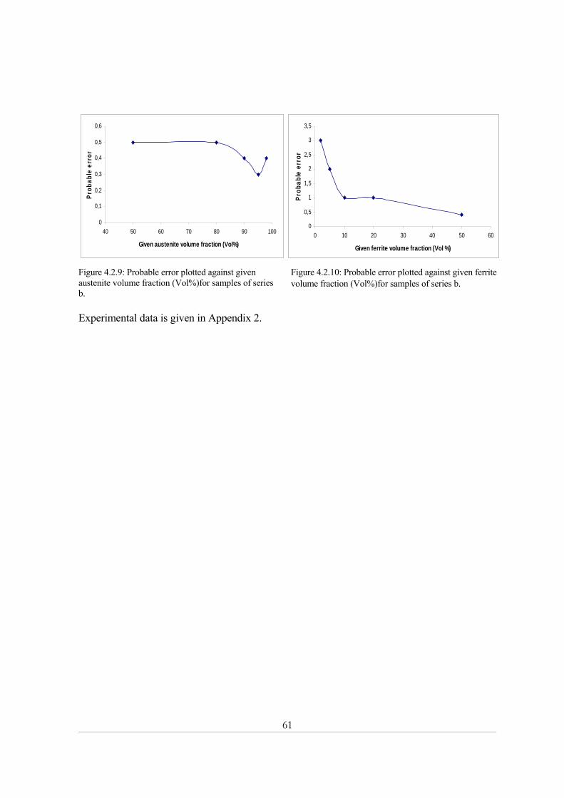
61

0

0,1

0,2

0,3

0,4

0,5

0,6

40 50 60 70 80 90 100

Given austenite volume fraction (Vol%)

Prob

able

err

or

0

0,5

1

1,5

2

2,5

3

3,5

0 10 20 30 40 50 60

Given ferrite volume fraction (Vol %)

Prob

able

err

or

Figure 4.2.9: Probable error plotted against given austenite volume fraction (Vol%)for samples of series b.

Figure 4.2.10: Probable error plotted against given ferrite volume fraction (Vol%)for samples of series b.

Experimental data is given in Appendix 2.

62

4.3- Electron backscatter diffraction (EBSD)

4.3.1 SEM micrograph A SEM micrograph and a SEM micrograph with EBSD map for both phases are given in figure

4.3.1(A) and (B), respectively. This step is the starting point for phase analysis with the help of

EBSD.

Figure. 4.3.1 The SEM micrograph (A) and the EBSD phase map with the SEM micrograph for comparison (B). Austenite is colored red and ferrite blue.

It can be seen that the mixture of ferrite and austenite is not homogenous. However, grains as

small as a few micrometers large can be identified. Both phases are almost separated from each

other. A close look at figure 4.3.1 B reveals that some material is not included in phase

identification and quantification. Consequently,

the computer software will consider this

material as pores during phase quantification.

4.3.2 EBSD Phase Map

EBSD phase quantitative analysis for sample 1-

b is shown in the figure 4.3.2.

2 The figure contains 1 map

Figure 4.3.2: EBSD Phase Map for sample 1-b2

A B

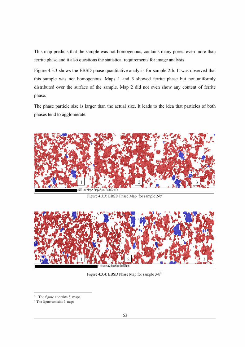
63

This map predicts that the sample was not homogenous, contains many pores; even more than

ferrite phase and it also questions the statistical requirements for image analysis

Figure 4.3.3 shows the EBSD phase quantitative analysis for sample 2-b. It was observed that

this sample was not homogenous. Maps 1 and 3 showed ferrite phase but not uniformly

distributed over the surface of the sample. Map 2 did not even show any content of ferrite

phase.

The phase particle size is larger than the actual size. It leads to the idea that particles of both

phases tend to agglomerate.

Figure 4.3.3: EBSD Phase Map for sample 2-b3

Figure 4.3.4: EBSD Phase Map for sample 3-b4

3 The figure contains 3 maps 4 The figure contains 3 maps

2 3 1

1 2 3

64

Figure 4.3.4 contains the EBSD phase quantitative analysis for sample 3-b. It was observed that

this sample was inhomogeneous. Although, all maps showed ferrite phase but not uniformly

distributed over the surface of the sample.

Figure 4.3.5: EBSD Phase Map for sample 4-b

EBSD phase quantitative analysis for sample 4-b is shown in the above figure. This sample was

inhomogeneous. Austenite particles formed zigzag patterns unlike ferrite phase particles. Ferrite

particles tend to agglomerate more than austenite. All maps showed ferrite phase but not

uniformly distributed over the surface of the sample.

Figure 4.3.6: EBSD Phase Map for sample 5-b5

Figure 4.3.6 shows the EBSD phase quantitative analysis for sample 5-b. The sample was

inhomogeneous. All maps showed ferrite and austenite phases but not uniformly distributed

5 The figure contains 3 maps

1 2 3

1 2 3

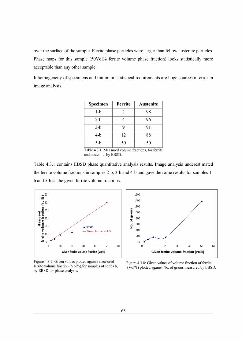
65

over the surface of the sample. Ferrite phase particles were larger than fellow austenite particles.

Phase maps for this sample (50Vol% ferrite volume phase fraction) looks statistically more

acceptable than any other sample.

Inhomogeneity of specimens and minimum statistical requirements are huge sources of error in

image analysis.

Specimen Ferrite Austenite 1-b 2 98 2-b 4 96

3-b 9 91 4-b 12 88

5-b 50 50 Table 4.3.1: Measured volume fractions, for ferrite and austenite, by EBSD.

Table 4.3.1 contains EBSD phase quantitative analysis results. Image analysis underestimated

the ferrite volume fractions in samples 2-b, 3-b and 4-b and gave the same results for samples 1-

b and 5-b as the given ferrite volume fractions.

0

10

20

30

40

50

60

0 10 20 30 40 50 60

Given ferrite volume fraction (Vol%)

Mea

sure

d fe

rrite

vol

ume

fract

ion

(Vol

%)

0

200

400

600

800

1000

1200

1400

1600

0 10 20 30 40 50 60

Given ferrite volume fraction (Vol%)

No.

of g

rain

s

Figure 4.3.7: Given values plotted against measured ferrite volume fraction (Vol%),for samples of series b, by EBSD for phase analysis.

Figure 4.3.8: Given values of volume fraction of ferrite (Vol%) plotted against No. of grains measured by EBSD.

♦EBSD ⎯ Given ferrite Vol %

66

Given and measured volume fractions of ferrite are plotted in the figure 4.3.7. EBSD analysis

gave quite accurate results for all samples, except for one sample, 4-b.

Statistically, there is a minimum limit on number of grains, which should be studied for image

analysis. Figure 4.3.8 gives a glimpse of the statistical side of EBSD results. It is apparent that

the number of grains decreases with decreasing volume fraction of second phase, which is

ferrite in this case. For low percentage of volume fraction of ferrite, the number of grains

measured was far below what is statistically required.

Experimental data is given in Appendix 3.

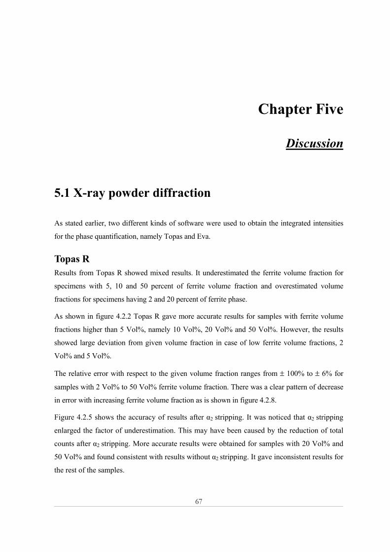
67

Chapter Five

Discussion

5.1 X-ray powder diffraction

As stated earlier, two different kinds of software were used to obtain the integrated intensities

for the phase quantification, namely Topas and Eva.

Topas R Results from Topas R showed mixed results. It underestimated the ferrite volume fraction for

specimens with 5, 10 and 50 percent of ferrite volume fraction and overestimated volume

fractions for specimens having 2 and 20 percent of ferrite phase.

As shown in figure 4.2.2 Topas R gave more accurate results for samples with ferrite volume

fractions higher than 5 Vol%, namely 10 Vol%, 20 Vol% and 50 Vol%. However, the results

showed large deviation from given volume fraction in case of low ferrite volume fractions, 2

Vol% and 5 Vol%.

The relative error with respect to the given volume fraction ranges from ± 100% to ± 6% for

samples with 2 Vol% to 50 Vol% ferrite volume fraction. There was a clear pattern of decrease

in error with increasing ferrite volume fraction as is shown in figure 4.2.8.

Figure 4.2.5 shows the accuracy of results after α2 stripping. It was noticed that α2 stripping

enlarged the factor of underestimation. This may have been caused by the reduction of total

counts after α2 stripping. More accurate results were obtained for samples with 20 Vol% and

50 Vol% and found consistent with results without α2 stripping. It gave inconsistent results for

the rest of the samples.

68

Topas P Results from Topas P also showed similar results. It also gave rise to an underestimation of the

ferrite volume fraction for specimens with 5 Vol% and 50 Vol% ferrite. However, it

overestimated ferrite fractions in rest of the specimens.

Figure 4.2.2 illustrates the deviation from given volume fractions of results obtained from

Topas P. Good accuracy in results was found for samples with higher ferrite volume fractions,

10 Vol%, 20 Vol% and 50 Vol%. Large deviation was observed, in case of low ferrite volume

fractions, 2 Vol% and 5 Vol%.

The relative error with respect to given volume fraction goes from ± 50% to ± 4%, for 2 Vol%

to 50 Vol% of ferrite, respectively. Topas P showed better accuracy than TopasR, although

Topas P gave results with an error, which decreases with increasing ferrite volume fraction.

Results from α2 stripping profiles are shown in figure 4.2.4. These results were consistent with

results obtained without α2 stripping, with the exception of the sample with 5 Vol% ferrite

fraction. It was also noticed that α2 stripping increased the factor of overestimation in case of

specimens with 5 Vol% ferrite fraction, only.

Eva Results from Eva showed a clear pattern of underestimation of ferrite volume fraction for all

specimens. The relative error with respect to given volume fraction goes from ± 50% to ± 8%

for samples with 2 Vol% to 50 Vol% ferrite.

According to figure 4.2.2 Eva gave more accurate results for samples with higher ferrite volume

fractions, 10 Vol%, 20 Vol% and 50 Vol% than for the samples with low ferrite volume

fractions, 2 Vol% and 5 Vol%.

The α2 stripping also showed similarity in result pattern, expect in case of the specimen with

20 Vol% ferrite phase. These results were much more consistent without α2 stripping than

both, Topas R and Topas P.

Specimens were also measured for full pattern phase analysis to determine the existence of

preferred orientation. The whole pattern analysis confirmed that these samples were free from

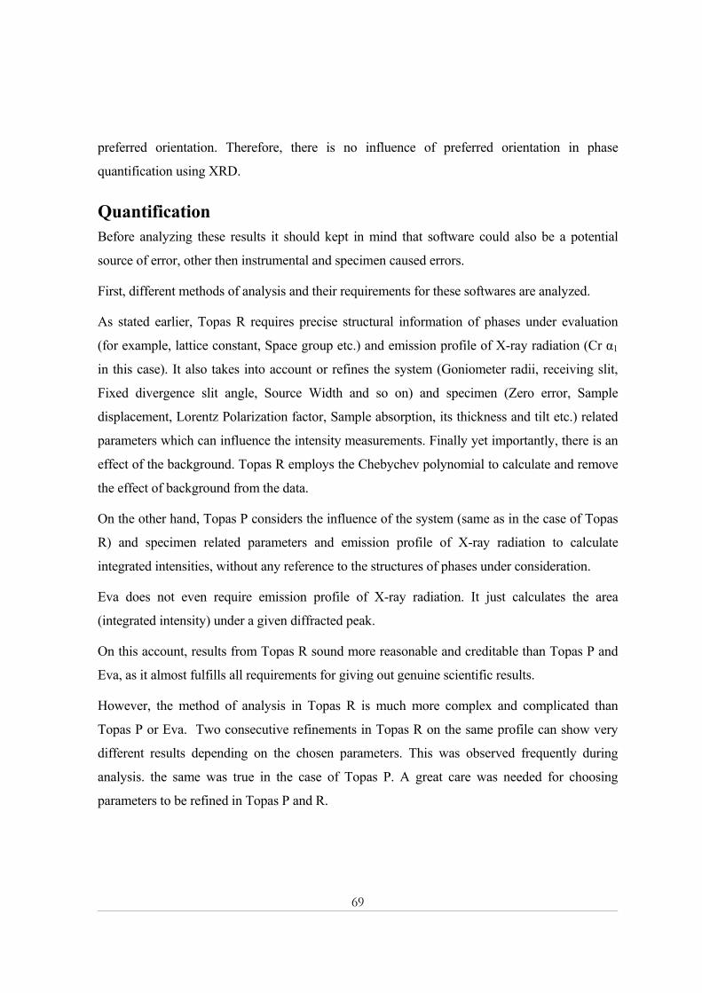
69

preferred orientation. Therefore, there is no influence of preferred orientation in phase

quantification using XRD.

Quantification Before analyzing these results it should kept in mind that software could also be a potential

source of error, other then instrumental and specimen caused errors.

First, different methods of analysis and their requirements for these softwares are analyzed.

As stated earlier, Topas R requires precise structural information of phases under evaluation

(for example, lattice constant, Space group etc.) and emission profile of X-ray radiation (Cr α1

in this case). It also takes into account or refines the system (Goniometer radii, receiving slit,

Fixed divergence slit angle, Source Width and so on) and specimen (Zero error, Sample

displacement, Lorentz Polarization factor, Sample absorption, its thickness and tilt etc.) related

parameters which can influence the intensity measurements. Finally yet importantly, there is an

effect of the background. Topas R employs the Chebychev polynomial to calculate and remove

the effect of background from the data.

On the other hand, Topas P considers the influence of the system (same as in the case of Topas

R) and specimen related parameters and emission profile of X-ray radiation to calculate

integrated intensities, without any reference to the structures of phases under consideration.

Eva does not even require emission profile of X-ray radiation. It just calculates the area

(integrated intensity) under a given diffracted peak.

On this account, results from Topas R sound more reasonable and creditable than Topas P and

Eva, as it almost fulfills all requirements for giving out genuine scientific results.

However, the method of analysis in Topas R is much more complex and complicated than

Topas P or Eva. Two consecutive refinements in Topas R on the same profile can show very

different results depending on the chosen parameters. This was observed frequently during

analysis. the same was true in the case of Topas P. A great care was needed for choosing

parameters to be refined in Topas P and R.

70

Statistical error Keeping all other result effecting factors constant, only one factor can discredit all the results.

This is statistical error.

The magnitude of probable error caused by statistical error depends upon the total number of

counts for a given time interval. During XRD intensity measurements, it was observed that it

ranges from 3% to 0.5% for samples with 2 Vol% to 50 Vol% ferrite phase, respectively.

According to figure 4.2.10 the statistical error rapidly decreases for samples with 2 Vol% to 10

Vol% ferrite and continue this tendency for samples with 20 Vol% and 50 Vol% ferrite as well.

The behavior of this curve helps to explain the XRD (Topas R, Topas P and Eva) results.

Samples with low ferrite fraction had high statistical error, which resulted in less accuracy in

results. And lower statistical error for samples with high ferrite volume fractions resulted in

good accuracy in their results. In other words, statistical error is directly related to the accuracy

of the results.

Theoretical intensities effect Theoretical intensities (R-values) needed for quantitative phase analysis by Topas P and Eva

can influence the results. The error caused by theoretical intensities could be as high as 1 %

[27].

Microabsorption and extinction, if present, can seriously reduce the accuracy of the direct

comparison method (used for phase quantification by Topas P and Eva), because this is an

absolute method. Fortunately, both effects are negligible in the case of hardened steel [3].

Therefore, the elimination of absorption coefficients of two-phases during approximations in

the direct comparison method did not affect the results.

Porosity effect Porosity of powder samples is also considered as a source of error in XRD analysis. Earlier

experiments have proven that the effect of porosity on results could be as large as 1% near the

theta value of 30 degrees, if the sample contains 50 Vol% pores [28].

In this work, the 2-theta range for two-peak analysis, one peak from each phase, was 64.5 to 71

degrees and for the whole pattern, analysis was 64.5 to 164.5 degrees. The number of pores in

71

the samples was much less then 50 Vol%. This was confirmed by images taken with backscatter

electron mode of SEM, as shown in appendix 3. Therefore, porosity of samples was not a

source of error in the XRD measurements.

Homogeneity of specimen EBSD analysis shows that the samples were not homogenous. Samples with low volume

fractions of ferrite were observed to be more inhomogeneous. This could be one factor, which

influences the phase quantification, particularly for low volume fractions, using XRD.

After reviewing the most probable sources of error in XRD quantitative analysis, statistical

error could be pointed out as the major factor, which affected the XRD measurements and

consequently the results. It is easy to look at the relation between probable statistical error and

error in XRD results. Both of them appreciably decrease with increase in ferrite volume

fraction.

Image analysis confirmed the inhomogeneity of samples. Other than statistical error,

homogeneity can also be a contributing factor in phase quantitative results for low volume

fractions.

According to figure 4.2.2 scatter in XRD results for samples 2 Vol%, 5 Vol% and 50 Vol%

ferrite fractions was much less than in the case of samples with 10 Vol% and 50 Vol% for

ferrite.

For samples with 2 Vol% ferrite volume fraction the relative error was up to ± 100%. Samples

with 5 Vol% and 10 Vol% ferrite volume fraction were found with relative error up to ± 40% of

given values. For samples with 20 and 50 Vol% ferrite volume fraction error was up to ± 4%,

with only one exception.

This concludes that as low as 2 Vol% of ferrite volume fraction can be detected with the help

of XRD, although with high statistical error.

72

5.2 Magnetic balance

Both Hoselite and Salwen formula were employed to calculate the magnetic volume fraction in

given specimen.

Results from Hoselitz formula showed very good accuracy. There was no relative error with

respect to the given volume fraction for samples with 2, 5 and 10 Vol% ferrite. But it ranges

from ± 5 % to ± 8% for samples with 20 Vol% to 50 Vol% ferrite.

Results from Salwen formula showed overestimation of ferrite volume fraction for almost all

specimens.

Reasons for such pattern of results rooted in the nature of these two formulas.

As stated earlier Salwen formula requires alloy composition of the whole specimen, which was

unknown in this case. And Hoselitz formula requires alloy composition of the magnetic phase

in the specimen. According to figure 4.1.4 the sigma M, calculated by Salwen’s formula, has

much higher value than sigma M, calculated by Hoselitz’s formula. The same pattern of

difference was observed in MB results. This highlights the “central position” of these formulas

for MB measurements. Unfortunately, both the Salwen and Hoselitz formulas are empirical

which means that there is no theoretical background for either of these formulas. This makes it

difficult to investigate the MB measurements in more detail.

5.3 Image analysis

Results from image analysis showed a large variation. It underestimated the amount of ferrite

volume fraction in case of samples with 5 Vol%, 10 Vol% and 20 Vol% ferrite phase. And

estimated the same as the given ferrite amount in case of samples with 2 Vol% and 50 Vol%

ferrite phase. The relative error with respect to given volume fraction goes from ± 20% to ±

40% for samples with 5 Vol% to 20 Vol% of ferrite, respectively. For samples with 2 Vol% and

50 Vol% ferrite phase the deviation was neglectable.

73

According to figure 4.3.7, image analysis measured the ferrite volume fractions for all samples

quite accurately, except in the case of 20 Vol% volume fraction, which deviates from the true

value by 40 % which is the largest relative error in comparison with the results by other

methods (36 % for Topas R; 20 % for Topas P; 5% Eva and 5 % for MB). This large deviation

could be caused by the insufficient sampling. Further work needs to be carried out in order to

find out the cause of this large deviation.

Image analysis can be subjected to different sources of error. For example, the representative

character of the sample, preferred orientation, inhomogeneity of sample, quality of sample

preparation and last but not least, the operator biasing.

All these factors are discussed one by one in the following text

It was observed that samples were not fully homogeneous and it could contribute to wrong

phase estimation. This effect becomes more significant for samples with low values of phase

fraction of ferrite phase, e.g. three EBSD maps are shown for a sample with 5 Vol% of ferrite

fraction in figure 4.3.5. Contents of both phases are scattered unevenly and one map does not

even have a single particle of ferrite phase.

Quality of sample preparation can seriously undermine the image analysis, for instance

excessive use of force during grinding and polishing could create pores in the samples. The

same thing was noticed during sample preparation for this work.

Porosity, if present, demands the measurement of large areas on the samples and estimation of

number of pores other than amount of phases under evaluation. It is an enormous problem when

working with low volume fractions. Figure 4.3.2 shows a large amount of pores, even more

than the ferrite contents in the sample.

Both XRD and EBSD confirmed that these samples were without any preferred orientation.

Statistical error can totally discard the results for phase quantification. The statistical

requirements suggest that measuring of at least 200 particles of the second phase is necessary

[26].

It was noticed that the statistical error increased with decreasing ferrite volume fraction. In case

of samples with 2 Vol% and 5 Vol% ferrite fraction the error can be as large as 100% (figure

74

4.3.2.). Therefore, for quantitative analysis a volume fraction ≥ 5 % is required in order to have

a relative error ≤ 20%.

The operator biasing is one of the dominant error factors in quantitative phase analysis using

image analysis. For example, selection of sample surface area, number of frames,

magnification, etc., all depend on operator or user. The user may also manipulate information to

obtain “desired” results.

Figure 4.3.3 is such an example. The map shows that the sample is not homogenous; powder

particles are bigger than the actual size, there is large porosity and high statistical error. In spite

of all these errors result is almost accurate except for 20 Vol% of ferrite.

Sample preparations, inhomogeneity of specimens, operator biasing and statistical error were all

observed during image analysis.

Results for samples with 2 Vol% and 5 Vol% ferrite fraction were possibly effected by the all

these factors described above. In case of samples with 10 Vol% and 20 Vol% ferrite a

reasonable statistical error was achieved but still the sample preparation and inhomogeneity of

samples could be contributing factors to underestimation. “Good” results were obtained in case

of samples with 2 Vol% and 50 Vol% ferrite phase.

Results dictate that as low as 2 Vol% of ferrite volume fraction can be detected and quantified,

although with high statistical error. With these possible errors results were found within the

absolute error range of ± 2%, except in the case of samples with 20 Vol% ferrite fraction.

5.4 Comparison

The XRD results, obtained using Topas R, P and Eva, were compared with each other.

Generally, results from Topas P and Eva were found more close to each other than Topas R. It

reflects the difference in their basic ways of phase quantification.

For sample with 2 Vol% ferrite volume fraction, Topas P and Eva estimated more accurately

than Topas R did. For sample with 5 Vol% ferrite volume fraction Topas P estimated more

accurately than Tops R and Eva.

75

For sample with 10 Vol% ferrite volume fraction Eva estimated more accurately than Topas R

and Topas P. For sample with 20 Vol% ferrite volume fraction, Topas P and Eva estimated

more accurately than Topas R did. For sample with 50 Vol% ferrite volume fraction all, three

showed almost similar results.

X-Ray Powder Diffraction

( relative error)

Ferrite (Vol %) Topas R Topas P Eva

Magnetic Balance

( relative error)

Image

Analysis ( relative error)

2 4 (100%) 3 (50%) 1 (50%) 2 6(0%) 2 (0%) 5 3 (40%) 5 (0%) 3 (40%) 5 (0%) 4 (20%) 10 7(30%) 14 (40%) 9 (10%) 10 (0%) 9 (10%) 20 27(35%) 24 (20%) 21 (5%) 19 (5%) 12 (40%) 50 47(6%) 48 (2%) 46(8%) 46 (8%) 50 (0%)

Table1: Results from all three experimental techniques.

Following facts surfaced when the results from all experimental techniques were compared.

Magnetic balance (MB) and image analysis (IA) gave accurate results for sample with 2 Vol%

ferrite volume fraction. High statistical error in this case could be the reason for wrong XRD

estimation.

XRD (Topas P) and MB gave accurate results for sample with 5 Vol% ferrite volume fraction.

High statistical error in both XRD (Topas R and Eva) and IA can be seen as the major factor for

wrong estimation. In IA some other factors like inhomogeneity and porosity can also act as

contributors to the error.

Only MB gave accurate results for sample with 10 Vol% ferrite volume fraction. Relatively

high statistical error in both XRD and IA can lead to wrong estimations. In IA some other

factors like inhomogeneity and porosity can also give errors.

XRD (Eva) and MB gave more accurate results than any other technique, in case of sample with

20 Vol% ferrite volume fraction. Besides inhomogeneity, porosity and relatively high statistical

error, operator biasing is the possible major source of error in this case for IA. Even with low

statistical error, Topas R and Topas P did not give good accuracy in results. The software effect,

6 Results obtained using Hoselitz formula

76

which is unknown, could be a reason for overestimation in this case. In this case, sigma M

(theoretical magnetic saturation) was the source of underestimation in MB result.

IA was the only technique, which gave accurate results for sample with 50 Vol% ferrite volume

fraction. The software effect could be the only possible source of underestimation in XRD

analysis. This is stated, because a relatively very low statistical error was observed in this case.

In this case, wrong estimation of sigma M was the source of error in MB result.

For low ferrite volume fractions, 2 Vol% and 5 Vol%, XRD analysis statistical error was the

dominant factor of error. For higher ferrite volume fractions, 10 Vol% and 20Vole%, both

statistical error and software effect ca be seen as error causing factors. Whereas in case of 50

Vol% ferrite fraction only the software effect can be named as source of error.

In MB analysis, “formula’s effect” can be underlined as the main source of underestimation in

case of 20 Vol% and 50 Vol% ferrite fractions. All results from IA were affected by

inhomogeneity, porosity, operator biasing and statistical error. Only results from 50 Vol%

satisfied the statistical

requirements.

Results from all techniques

give ± 2 % absolute error limit

for samples with 2 Vol% and 5

Vol% ferrite volume fraction.

For samples with 10 and 50

Vol% ferrite volume fraction

results were within the error

limit of ± 4%. An error limit

of ± 8% was observed in case

of sample with 20 Vol% ferrite

volume fraction.

0

10

20

30

40

50

60

0 10 20 30 40 50 60

Given volume fraction of ferrite (Vol%)

Mea

sure

d vo

lum

e fra

ctio

n of

ferr

ite (V

ol%

)

Figure 5.1: Graphical presentation of results.

⎯⎯ GGiivveenn ffeerrrriittee VVooll%% ♦♦TTooppaass––RR,, ■■ TTooppaass––PP,, ×× EEvvaa,, ▲▲ MMaagg..BBaallaannccee,, ҖҖ IImmaaggee AAnnaallyyssiiss

77

Chapter Six Conclusions

• Results, obtained from all three experimental techniques, were found within the absolute

error limit of ± 4% with respect to each other and “given” volume phase fractions.

• X-ray powder diffraction (XRD) was evaluated in detail. Influence of preferred

orientation, α2stripping, statistical error, porosity of samples and theoretical intensities

(R-values) on results were investigated. Experimental results obtained, using software

Eva, showed good accuracy.

• Statistical error was observed as the major source of error in XRD phase analysis, which

becomes more significant for low ferrite volume fractions.

• The XRD successfully detected and quantified ferrite volume fraction as low as 2 Vol%.

However, high statistical error was observed in case of 2 Vol% and 5 Vol% ferrite

volume fraction.

• Magnetic balance (MB) results have very good accuracy. Ferrite volume fraction as low

as 2 Vol% was quantified with MB.

• This work has illustrated the power of EBSD in comparison with BSE and EDX, for

quantitative phase analysis.

• Phase identification and quantification can be done with ease using EBSD. However,

the complete EBSD analysis is time consuming.

78

• Sample preparation (porosity), inhomogeneity and large statistical error (especially, for

low ferrite volume fraction) and operator biasing affected the IA results. Ferrite fraction

of 2 Vol% was quantified with IA, however with high statistical error.

• Powder based specimens were found free from preferred orientation, stress, and with

low level of porosity.

79

Chapter Seven Suggestions for future work

• More efforts must be made with respect to software Topas to find out its effect on the

results.

• The XRD system should be calibrated.

• Samples with low phase. volume fractions should be measured for long time intervals.

• Both Hoselitz and Salwen formula should be reassessed. The coefficients of alloying

elements, in these formulas, should be rechecked.

• For magnetic balance, chemical composition of both ferrite phase and specimen should

be experimentally determined, e.g. using WDS for the magnetic phase and wet chemical

method for the spacemen.

• EBSD analysis should be studied in detail because of its great potential for phase

analysis. However, sampling, specimen preparation and operator biasing should be kept

in mind.

• Homogenous specimens of duplex stainless steels with more phases, for example sigma

or carbides, should be fabricated and quantified.

80

81

References

1. Kar Lai Ng, Helen Lai Wa Chan, and Chung Loomg Choy, Piezoelectric and Pyroelectric Properties of the PZT/P (VDF-TrFE) composites with constituent Phases Poled in Parallet or Antiparallel Directions, IEEE,Vol.47,No. 6, Nov.2000.

2. S L YUAN, C S Xiong, ZY Li and Z C Xia, Phase separation and insulator –metal behavior in the highly Ba +2 doped La 1-xBa x MnO compounds, J.Physics. Condens. Matter 14(2002) 173-179.

3. H. W. Hayden and S. Floreen, The Fatigue behavior of Fine Grained Two-Phase Alloys, Met. Trans.:Vol.4, Feb. 73.

4. Kazuyuki Handa, Yoshisato Kimura and Yoshinao Mishima, Microstructures and mechanical properties of the γ/k two-phase Fe-Mn-Al-c (-Cr) alloys, Mat.Res.Soc.Symp.Proc.Vol.646, 2001.

5. B.D Cullity ,Elements of x-ray diffraction , Second Edition.

6. Jan B. Ridenfeldt, 1988, Stainless steel Metal Matrix Composite.

7. Hedebrant, Olle: Magnetisk vag for matning av magnetiska momentet hos ferromagnetiska materal, Jernkontorets Annaloer arg 138 H10.1954.

8. Marai Jacobsson and Tomas Thorvaldsson, 1990 .Measurement of magnetic phase in the magnetic balance.

9. ASM hand book

10. Standard Test Method for Determining Volume Fraction by Systematic Manual Point Count.

11. G.F vander Voort, International Conference on Quantitative Microdcopy and image analysis, 1993. Precision and reproducibility of quantitative measurements .

12. G.S.Cole, International Conference on Quantitative Microdcopy and image analysis, 1993. Theory and Concepts for Computer –Aided Microscopy .

13. Wilson, Lönnberg:Fashaltsmätning med magnetvåg,SE11T005646,1989.

82

14. Jonsson, P-E: Feluppskattning och korrektion av fjädervåg för bestämning av magnetisk fas, IT001676, 1976.

15. Claes-Ove, Pettersson and Sven –Åke Fager, Welding practice for the Sandvik Duplex stainless steels.

16. Guocai ,Chai and Magnus Nyström ,Mechanical properties of Sandvik SAF2205 and Sandvik SAF2507 .

17. H. Vannevik, J.-o. Nilsson, J. Frodigh and P. Khangas, Effect of elemental partitioning on pitting resistance of high nitrogen duplex stainless steels, ISIJ, Vol. 36(1996),No. 7(July)

18. Johan frodign and j. Michael Nicholls, Mechanical properties of Sandvik duplex stainless steels.

19. Experience on contrasting microstructure using Orientation imaging microscopy, Danka, ClaudimDanial, Frank, Prakt. Metallogr. 35 (1998)

20. ASTM E975-03

21. TOPAS user’s manual

22. David Brandon and Wayne D. Kaplan , Microstructure characterization of materials.

23. ASTM E 975-03

24. R.L. Snyder & D.L.Bish

25. ASTM 1245-03

26. Retained Austenite and its Measurements by X ray diffraction, SP-453,1980.

27. P.Trucano and B.W. Batterman, Effect of porosity in powder diffraction, J. A. Physics Vol.41,10, 1970.

28. Harold P. Klug and Leroy E. Alexander. X -ray diffraction Procedures, Second edition, J Willy & Sons, New York.

29. Sandvik steel sales training manual.

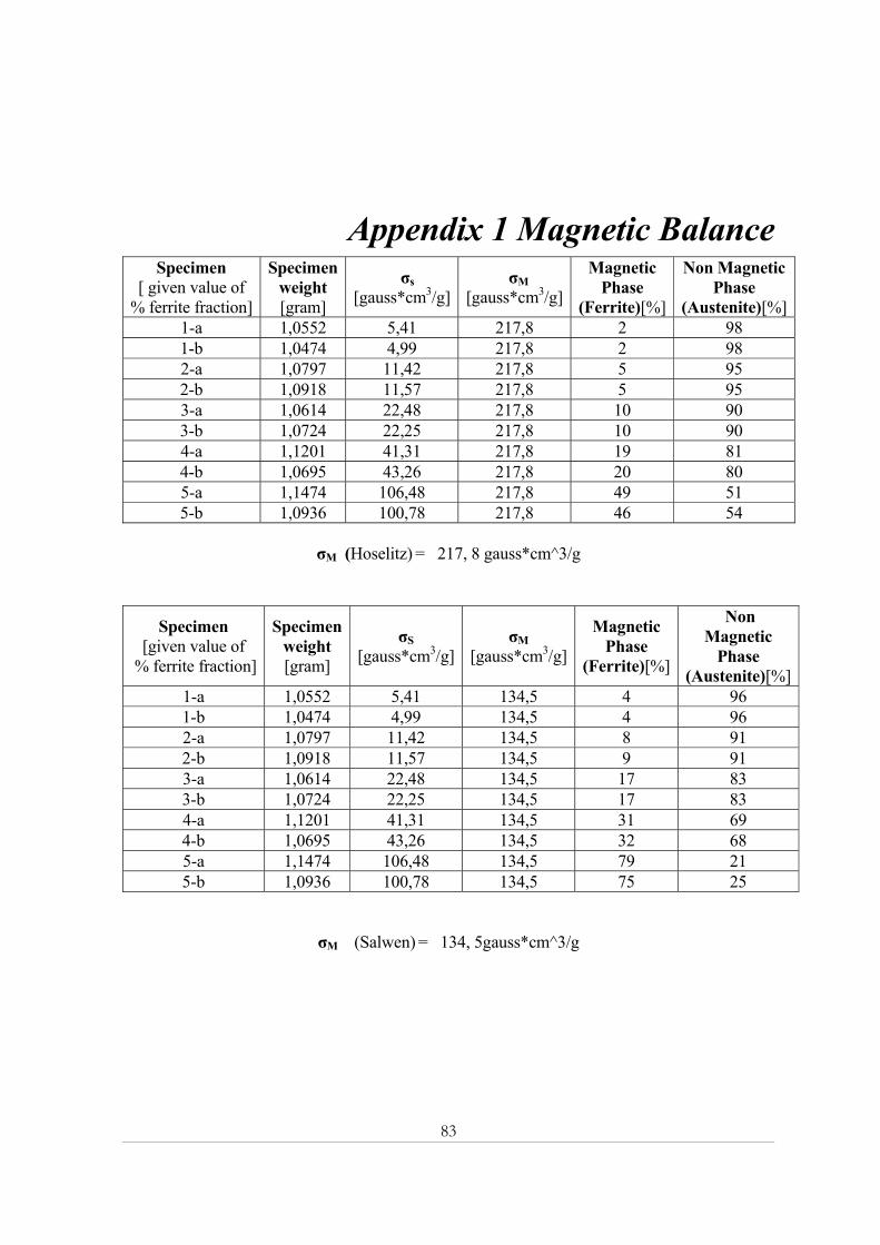
83

Appendix 1 Magnetic Balance Specimen

[ given value of % ferrite fraction]

Specimen weight [gram]

σs [gauss*cm3/g]

σM [gauss*cm3/g]

Magnetic Phase

(Ferrite)[%]

Non Magnetic Phase

(Austenite)[%]1-a 1,0552 5,41 217,8 2 98 1-b 1,0474 4,99 217,8 2 98 2-a 1,0797 11,42 217,8 5 95 2-b 1,0918 11,57 217,8 5 95 3-a 1,0614 22,48 217,8 10 90 3-b 1,0724 22,25 217,8 10 90 4-a 1,1201 41,31 217,8 19 81 4-b 1,0695 43,26 217,8 20 80 5-a 1,1474 106,48 217,8 49 51 5-b 1,0936 100,78 217,8 46 54

σM (Hoselitz) = 217, 8 gauss*cm^3/g

Specimen [given value of

% ferrite fraction]

Specimen weight [gram]

σS [gauss*cm3/g]

σM [gauss*cm3/g]

Magnetic Phase

(Ferrite)[%]

Non Magnetic

Phase (Austenite)[%]

1-a 1,0552 5,41 134,5 4 96 1-b 1,0474 4,99 134,5 4 96 2-a 1,0797 11,42 134,5 8 91 2-b 1,0918 11,57 134,5 9 91 3-a 1,0614 22,48 134,5 17 83 3-b 1,0724 22,25 134,5 17 83 4-a 1,1201 41,31 134,5 31 69 4-b 1,0695 43,26 134,5 32 68 5-a 1,1474 106,48 134,5 79 21 5-b 1,0936 100,78 134,5 75 25

σM (Salwen) = 134, 5gauss*cm^3/g

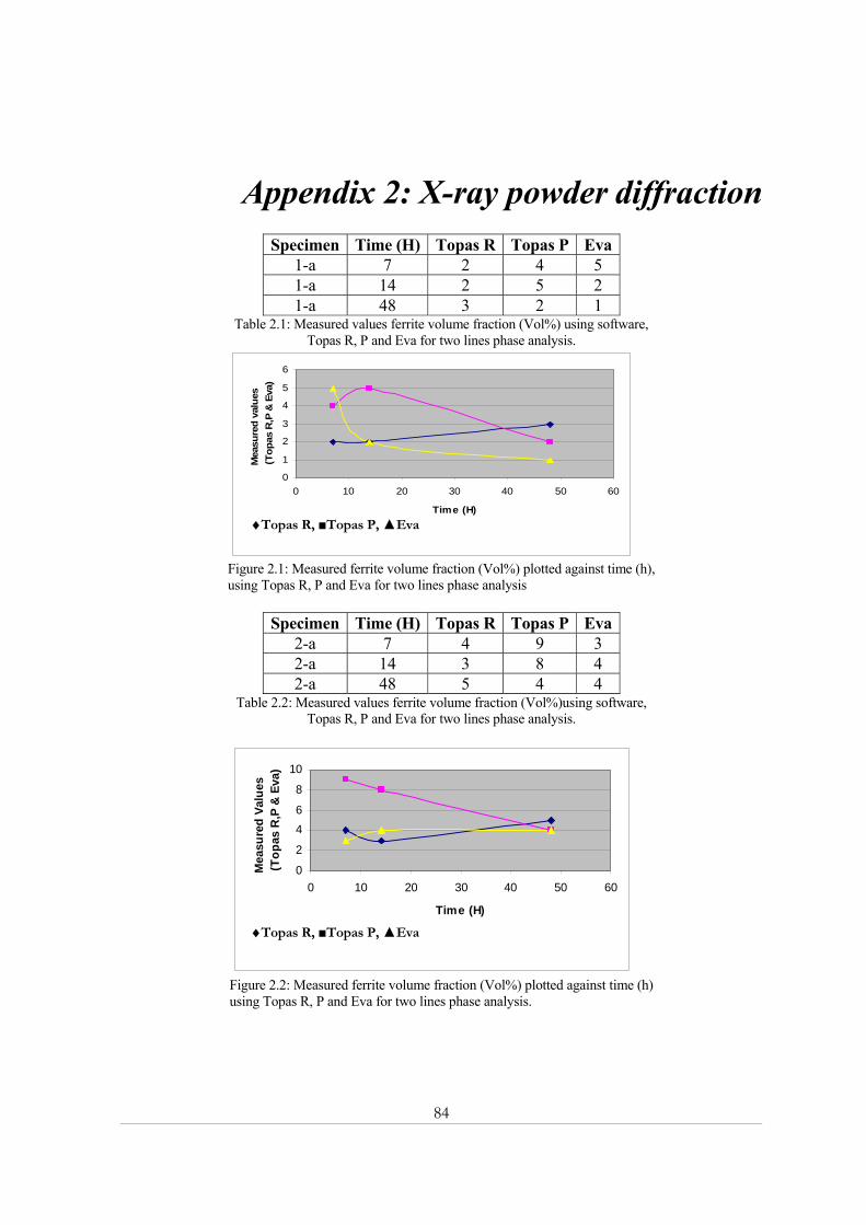
84

Appendix 2: X-ray powder diffraction

Specimen Time (H) Topas R Topas P Eva1-a 7 2 4 5 1-a 14 2 5 2 1-a 48 3 2 1

Table 2.1: Measured values ferrite volume fraction (Vol%) using software, Topas R, P and Eva for two lines phase analysis.

0

1

2

3

4

5

6

0 10 20 30 40 50 60

Time (H)

Mea

sure

d va

lues

(T

opas

R,P

& E

va)

Figure 2.1: Measured ferrite volume fraction (Vol%) plotted against time (h), using Topas R, P and Eva for two lines phase analysis

Specimen Time (H) Topas R Topas P Eva

2-a 7 4 9 3 2-a 14 3 8 4 2-a 48 5 4 4

Table 2.2: Measured values ferrite volume fraction (Vol%)using software, Topas R, P and Eva for two lines phase analysis.

0

2

46

8

10

0 10 20 30 40 50 60

Time (H)

Mea

sure

d Va

lues

(T

opas

R,P

& E

va)

Figure 2.2: Measured ferrite volume fraction (Vol%) plotted against time (h) using Topas R, P and Eva for two lines phase analysis.

♦Topas R, ■Topas P, ▲Eva

♦Topas R, ■Topas P, ▲Eva

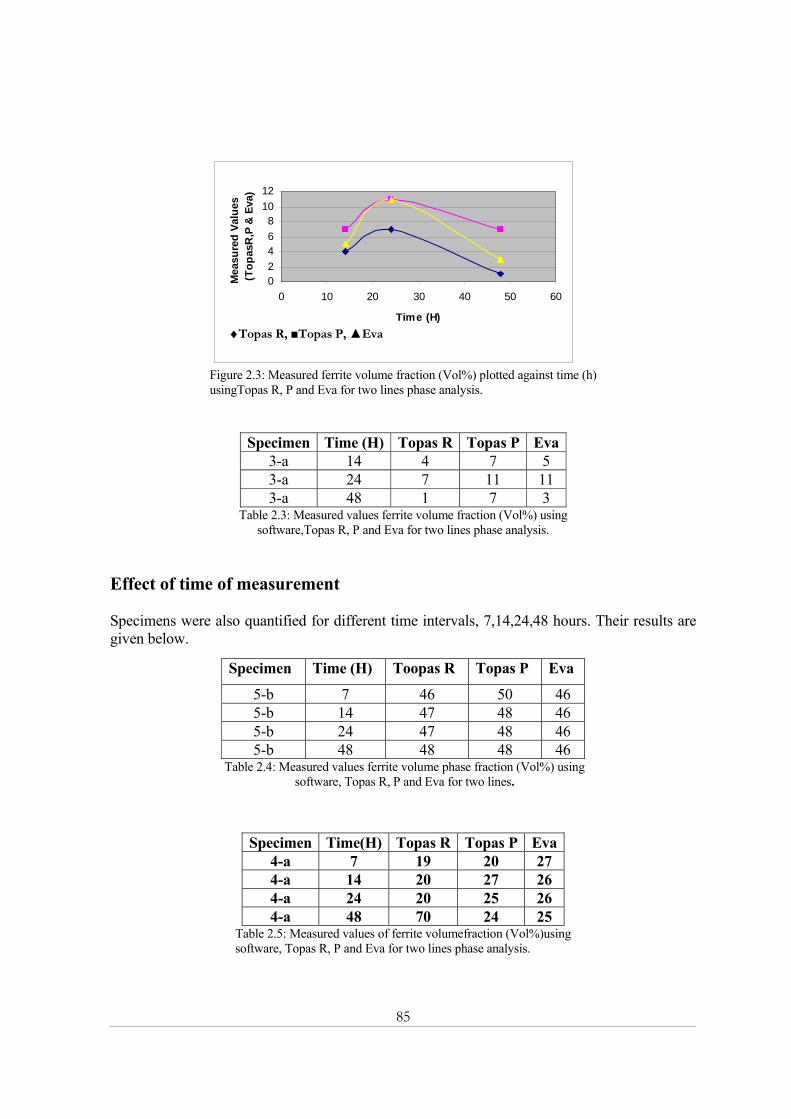
85

02468

1012

0 10 20 30 40 50 60

Time (H)

Mea

sure

d Va

lues

(T

opas

R,P

& E

va)

Figure 2.3: Measured ferrite volume fraction (Vol%) plotted against time (h) usingTopas R, P and Eva for two lines phase analysis.

Specimen Time (H) Topas R Topas P Eva3-a 14 4 7 5 3-a 24 7 11 11 3-a 48 1 7 3

Table 2.3: Measured values ferrite volume fraction (Vol%) using software,Topas R, P and Eva for two lines phase analysis.

Effect of time of measurement Specimens were also quantified for different time intervals, 7,14,24,48 hours. Their results are given below.

Specimen Time (H) Toopas R Topas P Eva

5-b 7 46 50 46 5-b 14 47 48 46 5-b 24 47 48 46 5-b 48 48 48 46

Table 2.4: Measured values ferrite volume phase fraction (Vol%) using software, Topas R, P and Eva for two lines.

Specimen Time(H) Topas R Topas P Eva4-a 7 19 20 27 4-a 14 20 27 26 4-a 24 20 25 26 4-a 48 70 24 25

Table 2.5: Measured values of ferrite volumefraction (Vol%)using software, Topas R, P and Eva for two lines phase analysis.

♦Topas R, ■Topas P, ▲Eva

86

45,546

46,547

47,548

48,549

49,550

50,5

0 10 20 30 40 50 60

Time (H)

Mea

sure

d Va

lues

(T

opas

R,P

& E

va)

Figure 2.4: Measured of ferrite volume fractions (Vol%) plotted against time (h) ,using Topas R, P and Eva for two lines phase analysis.

0

5

10

15

20

25

30

0 10 20 30 40 50 60

Time (H)

Mea

sure

d Va

lues

(T

opas

R,P

& E

va)

Figure 2.8: Measured ferrite volume fractions (Vol%) plotted against time (h),using Topas R, P and Eva for two lines phase analysis.

00,5

11,5

22,5

33,5

44,5

0 10 20 30 40 50 60

Time (H)

Prob

. err

or

Figure 2.9: Probable error plotted against Time (H) for sample (4-a)

Topas RTopas P Eva

ferrite phase austenite phase

Topas R, Topas P, Eva

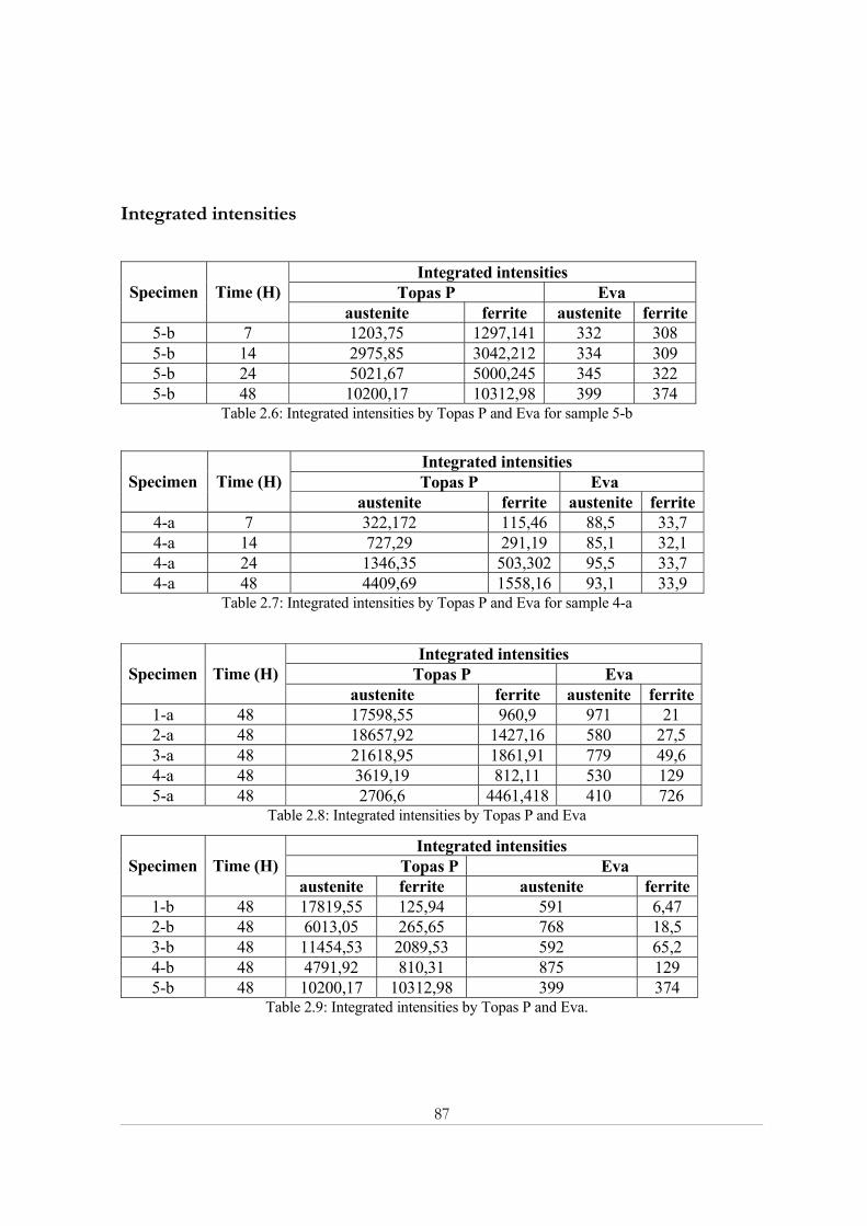
87

Integrated intensities

Integrated intensities Topas P Eva Specimen Time (H)

austenite ferrite austenite ferrite 5-b 7 1203,75 1297,141 332 308 5-b 14 2975,85 3042,212 334 309 5-b 24 5021,67 5000,245 345 322 5-b 48 10200,17 10312,98 399 374

Table 2.6: Integrated intensities by Topas P and Eva for sample 5-b

Integrated intensities Topas P Eva Specimen Time (H)

austenite ferrite austenite ferrite 4-a 7 322,172 115,46 88,5 33,7 4-a 14 727,29 291,19 85,1 32,1 4-a 24 1346,35 503,302 95,5 33,7 4-a 48 4409,69 1558,16 93,1 33,9

Table 2.7: Integrated intensities by Topas P and Eva for sample 4-a

Integrated intensities Topas P Eva Specimen Time (H)

austenite ferrite austenite ferrite 1-a 48 17598,55 960,9 971 21 2-a 48 18657,92 1427,16 580 27,5 3-a 48 21618,95 1861,91 779 49,6 4-a 48 3619,19 812,11 530 129 5-a 48 2706,6 4461,418 410 726

Table 2.8: Integrated intensities by Topas P and Eva Integrated intensities

Topas P Eva Specimen Time (H) austenite ferrite austenite ferrite

1-b 48 17819,55 125,94 591 6,47 2-b 48 6013,05 265,65 768 18,5 3-b 48 11454,53 2089,53 592 65,2 4-b 48 4791,92 810,31 875 129 5-b 48 10200,17 10312,98 399 374

Table 2.9: Integrated intensities by Topas P and Eva.

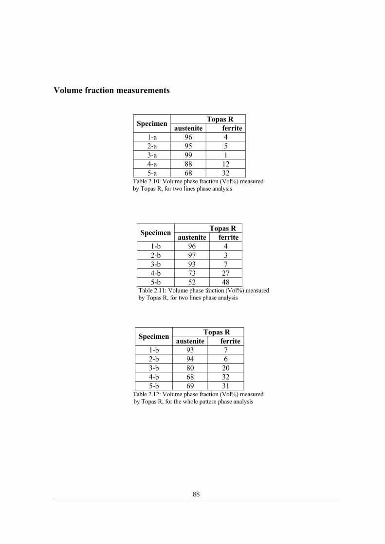
88

Volume fraction measurements

Topas R Specimen austenite ferrite1-a 96 4 2-a 95 5 3-a 99 1 4-a 88 12 5-a 68 32

Table 2.10: Volume phase fraction (Vol%) measured by Topas R, for two lines phase analysis

Topas R Specimen austenite ferrite1-b 96 4 2-b 97 3 3-b 93 7 4-b 73 27 5-b 52 48

Table 2.11: Volume phase fraction (Vol%) measured by Topas R, for two lines phase analysis

Topas R Specimen austenite ferrite1-b 93 7 2-b 94 6 3-b 80 20 4-b 68 32 5-b 69 31

Table 2.12: Volume phase fraction (Vol%) measured by Topas R, for the whole pattern phase analysis

89

Statistical error

Austenite Specimen NB NPB NP = NBP – NB Probable error 1-a 1417 39123 37706 0,3 2-a 1280 31902 30623 0,4 3-a 1711 39629 37918 0,3 4-a 262,5 5243 4980,5 1 5-a 1201 18948 17747 0,5

Table 2.13: Statistical error calculation for the austenite phase.

Ferrite Specimen NB NPB NP = NBP – NB Probable error

1-a 1280 1828 548 3 2-a 1234 2834 1600 2 3-a 1711 4593 2882 1 4-a 252 2433 2181 1 5-a 1201 36384 35183 0,4

Table 2.14: Statistical error calculation for the ferrite phase.

Austenite Specimen NB NPB NP = NBP – NB Probable error

1-b 1091 28883 28883 0,4 2-b 1815 43056 43056 0,3 3-b 1249 31244 31244 0,4 4-b 997 22022 22022 0,5 5-b 1139 18344 18344 0,5 Table 2.15: Statistical error calculation for austenite phase.

Ferrite

Specimen NB NPB NP = NBP – NB Probable error 1-a 982 1528 546 3 2-a 1664 3025 1361 2 3-a 1224 5327 4103 1 4-a 1092 8163 7071,5 1 5-a 1111 20110 18999 0,4 Table 2.16: Statistical error calculation for the ferrite phase.

90

Austenite Specimen Time (H) NB NPB NP = NBP – NB Probable error

5-b 7 180 2660 2480 1 5-b 14 350 5204 4854 1 5-b 24 560 9736 9177 1 5-b 48 1139 18344 17205 0,5

Table 2.17: Statistical error calculation for the austenite phase.

Ferrite

Specimen Time (H) NB NPB NP = NBP – NB Probable error 5-b 7 156 2876 2720 1 5-b 14 378 5595 5217 1 5-b 24 615 10351 9736 1 5-b 48 1111 20110 18999 0,4

Table 2.18: Statistical error calculation for the ferrite phase.

Austenite

Specimen Time (H) NB NPB NP = NBP – NB Probable error 2-a 7 64 779 716 2,5 2-a 14 85 1498 1413 2 2-a 24 133 2915 2783 1 2-a 48 263 5243 4981 1

Table 2.19: Statistical error calculation for the austenite phase.

Ferrite Specimen Time (H) NB NPB NP = NBP – NB Probable error

2-a 7 79,5 350 270,5 4 2-a 14 102 664 562 3 2-a 24 162 1212 1050 2 2-a 48 252 2433 2181 1,4

Table 2.20: Statistical error calculation for the ferrite phase.

91

Time of measurement

Above Figure shows the XRD profiles of sample 5-b measured for different time intervals. The

number of counts increases with increasing time of measurements.

Figure 2.10: Observed XRD profiles of sample 5-b measured for different time intervals.

92

Appendix 3 Image analysis

Specimen Number of Grains Austenite phase Ferrite phase

1-b 1895 5 2-b 3933 87 3-b 3761 164 4-b 2823 154 5-b 3004 1376

Table 3.1: Number of grains from each phase considered for image analysis.

Figure 3.1: Backscatter electron image for a sample with 50% ferrite volume fraction.

93

Figure 3.2: Energy dispersive X rays (EDX) map for austenite phase; sample with 50% ferrite volume fraction.

Figure 3.2: Energy dispersive X rays (EDX) map for ferrite phase; sample with 50% ferrite volume fraction.

94

Department of Physics and Measurement Technology

Datum Date 2004-12-21

Språk Language Svenska/Swedish x Engelska/English _____________

Rapporttyp Report category Licentiatavhandling x Examensarbete C-uppsats D-uppsats Övrig rapport __________

ISBN _____________________________________________ ISRN _____________________________________________ Serietitel och serienummer ISSN Title of series, numbering

LITH-IFM-EX--04/1358—SE

URL för elektronisk version

Titel Title Quantitative analysis of multi-phase systems –steels with mixture of ferrite and austenite. Författare Author Fawad Salman Khokhar

Sammanfattning Abstract The goal of this work has been to evaluate the different experimental techniques used for quantitative analysis of multi-phase materials systems. Powder based specimens containing two-phases, austenite (γ) and ferrite (α), were fabricated and quantified. The volume fraction of ferrite varied from 2 Vol% to 50 Vol%. X ray powder diffraction (XRD) measurements were based on two peak analysis. Computer based software Topas was used for quantitative analysis, which is believed to be the most advanced in this field. XRD results were found within the absolute limit of ± 4% of given ferrite volume fraction. Volume fraction as low as 2 Vol% was successfully detected and quantified using XRD. However, high statistical error was observed in case of low volume fraction, such as 2 Vol% and 5 Vol% ferrite volume fraction. Magnetic balance (MB) measurements were performed to determine the volume fraction of magnetic phase, ferrite. MB results were found in good agreement with given volume fractions. As low as 2 Vol% volume fraction was detected and quantified with MB. MB results were within the absolute limit of ± 4% of given ferrite volume fraction. Image analysis (IA) was performed after proper sample preparation as required by electron backscatter diffraction (EBSD) mode of Scanning electron microscopy (SEM). IM results were found within the absolute limit of ± 2 % of given ferrite volume fraction. However, high statistical error was observed in case of 2 Vol% volume fraction.

Nyckelord Keyword Quantitative analysis, X-ray powder diffraction, Electron backscatter diffraction, Magnetic balance, Topas, Austenite (γ) and Ferrite (α) steels.

Avdelning, Institution

95