quantifying uncertainty through position analysis in ... sessions... · quantifying uncertainty...
TRANSCRIPT

Quantifying Uncertainty through Position
Analysis in Drought Water Supply Planning:
Examples from California
Tom FitzHugh
Supervising Water Resources Scientist

• Background on Central Valley Water Supply
Operations
• CalSim 2 Model
• Use of Position Analysis in Water Supply Planning
• Example: San Joaquin Flow Objectives Position
Analysis
• Forecast-Based Modeling for Water Supply
Planning
• Conclusion
2

Central Valley Project &
State Water Project Features
Description
Central
Valley
Project
State
Water
Project
Storage Facilities
Number 20 20
Storage (TAF) 11,000 5,800
Hydropower Facilities
Number 11 8
Generation Capacity
(Megawatts)2,100 1,380
Land UseIrrigable Lands
(million acres)
2.6 0.75
Direct Beneficiaries
Water Contractors >250 29
Power Contractors 60 -

Central Valley Project &
State Water Project FeaturesCVP and SWP
System Schematic

5
• Decline in health of Delta and riverine ecosystems has led
to increasing environmental regulations, most recently the
2008-2009 Biological Opinions

6
• Growth of snowpack and storage throughout winter allows
for prediction of water supply availability
• Midway through water year initial water supply allocation is
developed, then refined through May
– SWP – January through May
– CVP – February through May
• Exceedance probabilities used for inflow forecasts
– CVP – Feb 99%, Mar 90%, Apr 75%, May 50%
– SWP – Jan-Mar 99%, Apr-May 90%
• Allocation accounts for water to be delivered while
retaining carryover storage for future years
7
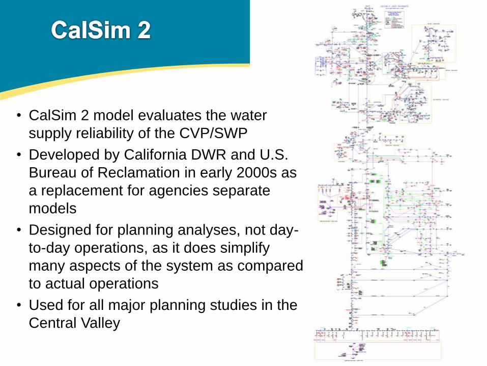
• CalSim 2 model evaluates the water
supply reliability of the CVP/SWP
• Developed by California DWR and U.S.
Bureau of Reclamation in early 2000s as
a replacement for agencies separate
models
• Designed for planning analyses, not day-
to-day operations, as it does simplify
many aspects of the system as compared
to actual operations
• Used for all major planning studies in the
Central Valley

8
• CalSim 2 is a specific application generated using a generic
modeling system developed by California DWR (WRIMS)
• Simulates all major features of system in Valley:
– reservoirs and water supply facilities
– river flows and Delta flows and salinity
– environmental regulations
– deliveries under contracts and water rights.
• Monthly model: Period of record 1922-2003
• Operated at a fixed level of development under a consistent
regulatory regime
• Hydrologic inputs represent flows that historical climate
conditions would have produced under current or future
levels of development

9
• Example applications
– Storage projects (EISs and Feasibility Reports)
– Water Control Manual updates
– SWP Delivery Capability Report
– Studies of climate change impacts
– Reclamation long-term operations studies
– Environmental and water supply permitting
• Often used to provide inputs/boundary conditions for other
models (temperature, economics, water quality)
• Versions do exist that are used for annual water supply
planning

10
• 82 one year model runs using each annual year of inflows from
1922-2003
• Conducted early in water year (October) when ability to forecast
flows is very low
• Model initialized with conditions at end of September (i.e
reservoir storages, prior month flows, etc.)
• Results capture the range of possible future operations and
deliveries that would occur under the historical range of
hydrologic conditions

11

12
• Seasonal variability of inflows will affect operations
• Snowmelt flows in spring more predictable than rainfall in winter

13
• Examples of operations following:
– 2011: Very wet year
– 2013-2015: 3 consecutive drought years

14
Annual CVP South of Delta Deliveries

15
16
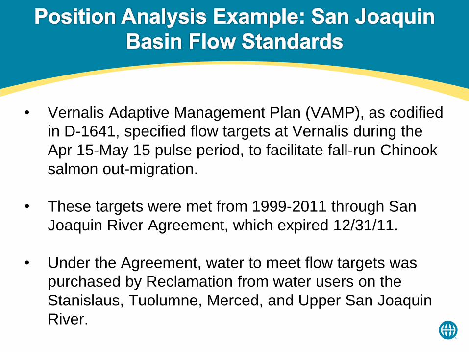
• Vernalis Adaptive Management Plan (VAMP), as codified
in D-1641, specified flow targets at Vernalis during the
Apr 15-May 15 pulse period, to facilitate fall-run Chinook
salmon out-migration.
• These targets were met from 1999-2011 through San
Joaquin River Agreement, which expired 12/31/11.
• Under the Agreement, water to meet flow targets was
purchased by Reclamation from water users on the
Stanislaus, Tuolumne, Merced, and Upper San Joaquin
River.
17
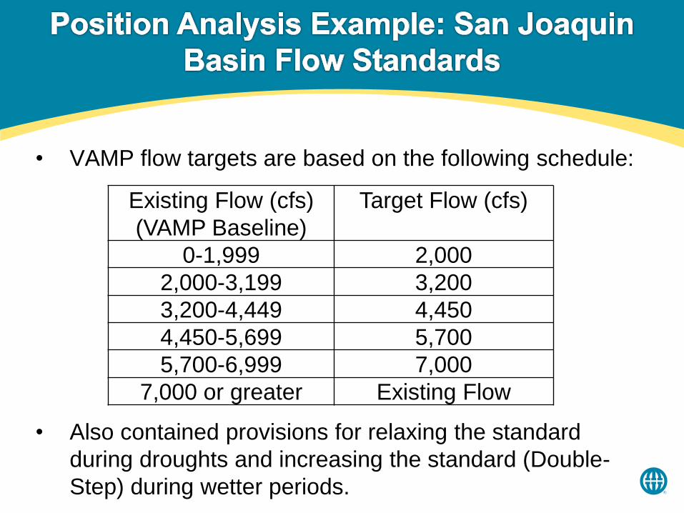
• VAMP flow targets are based on the following schedule:
• Also contained provisions for relaxing the standard
during droughts and increasing the standard (Double-
Step) during wetter periods.
Existing Flow (cfs)
(VAMP Baseline)
Target Flow (cfs)
0-1,999 2,000
2,000-3,199 3,200
3,200-4,449 4,450
4,450-5,699 5,700
5,700-6,999 7,000
7,000 or greater Existing Flow

18
• Two-year window (2012-2013) after expiration of VAMP
standard but before implementation of a long-term flow
standard by the CA State Water Resources Control
Board (SWRCB).
• Modeling conducted to support Reclamation’s
negotiations with water users for purchase of water to
meet VAMP-like flow targets over this two-year period.
• Led to agreement with Merced Irrigation District for
purchase of water to meet single-step VAMP standards

19

20
• Comparison of actual VAMP
contributions during 1999-2010 to
CalSim 2 modeled contributions
over 82 year model run (with
assumptions similar to historical
conditions).
• Boxplots very similar. Wilcoxon
rank-sum test p-value = 0.76, so
no statistically significant
difference.0
20
40
60
80
100
120
140
Actual CalSim
TA
F
VAMP contributions

21
0
5000
10000
15000
20000
25000
30000
0%20%40%60%80%100%Fl
ow
(cfs
)Percent Exceedance
Vernalis spring pulse period flows - Wet Years
Proposed Action
No Action

22
0
2000
4000
6000
8000
10000
12000
0%20%40%60%80%100%Fl
ow
(cfs
)Percent Exceedance
Vernalis spring pulse period flows - Above Normal/Below Normal Years
Proposed Action
No Action

23
0
2000
4000
6000
8000
10000
12000
0%20%40%60%80%100%Fl
ow
(cfs
)Percent Exceedance
Vernalis spring pulse period flows - Dry/Critical Years
Proposed Action
No Action

24
0
10
20
30
40
50
60
70
80
90
100
0%20%40%60%80%100%A
nn
ual
re
leas
es
(taf
)
Percent Exceedance
Contributions to meeting VAMP single-step target under the
Proposed Action
Lake McClure release to meet single-step VAMP target
New Melones releases to meet the Stanislaus RPA above other instream flow standards

250
20
40
60
80
Critical Dry Below Normal Above Normal Wet
TA
F
Purchase amounts - 2nd year
0
20
40
60
80
Critical Dry Below Normal Above Normal Wet
TA
F
Purchase amounts - 1st year

26
• Limitation of Position Analysis is that it is only useful at the
beginning of the water year
• Once there is snowpack in the mountains, all historical runoff
patterns are not equally likely
• Alternative approach is to run model using flow forecasts
• Data available to do this from California Nevada River Forecast
Center (CNRFC)
• Modified CalSim 2 to replace historically-based inflows with
inflows from CNRFC forecasts
• Model can be run starting in any month October-May, for one
year, under 5 exceedance forecasts (10%, 25%, 50%, 75%,
90%)
27
CNRFC Forecasts:
• Generated using National Weather Service River Forecast
System, a collection of data processing tools and hydrologic
simulation models
• Model is run for one year starting from current date for all
calibration datasets (30-40 years), producing a series of traces
• Exceedance values derived from these traces are published
daily on the internet
• Forecasts are unimpaired runoff, so in many cases need to be
statistically converted to estimates of actual inflows into
reservoirs

28

29
• Forecast locations needed
to run CalSim 2 shown in
map
• These mostly are rim
inflows to major reservoirs
• Forecasts statistically
converted into inflows to
reservoirs and also
accretion-depletion terms
and agricultural demands
CNRFC Forecast
Locations

30
Run Process

31
Shasta monthly storage, from forecast-based run
conducted in December 2015

32
Shasta monthly storage, from forecast-based run
conducted in April 2016

33
CVP South of Delta Deliveries in July, from
forecast-based run conducted in December 2015

34
• CalSim 2 model provides multiple methods for analyzing
uncertainty in annual water supply planning
– Position analysis to simulate range of possible operations from
beginning of water year (October)
– Forecast-based analysis to evaluate changes in operations
throughout water year (October – May)
• Further work to be conducted validating forecast-based
CalSim 2 model compared to historical water supply
operations
