HAL Id: hal-01103644https://hal.archives-ouvertes.fr/hal-01103644v2

Submitted on 12 Apr 2016

HAL is a multi-disciplinary open accessarchive for the deposit and dissemination of sci-entific research documents, whether they are pub-lished or not. The documents may come fromteaching and research institutions in France orabroad, or from public or private research centers.

L’archive ouverte pluridisciplinaire HAL, estdestinée au dépôt et à la diffusion de documentsscientifiques de niveau recherche, publiés ou non,émanant des établissements d’enseignement et derecherche français ou étrangers, des laboratoirespublics ou privés.

Copyright

Quantifying uncertainties on excursion sets under aGaussian random field prior

Dario Azzimonti, Julien Bect, Clément Chevalier, David Ginsbourger

To cite this version:Dario Azzimonti, Julien Bect, Clément Chevalier, David Ginsbourger. Quantifying uncertainties onexcursion sets under a Gaussian random field prior. SIAM/ASA Journal on Uncertainty Quantifi-cation, ASA, American Statistical Association, 2016, 4 (1), pp.850-874. �10.1137/141000749�. �hal-01103644v2�

Quantifying uncertainties on excursion sets under

a Gaussian random field prior

Dario Azzimonti ∗, Julien Bect †, Clement Chevalier ‡, David Ginsbourger§∗

Abstract

We focus on the problem of estimating and quantifying uncertaintieson the excursion set of a function under a limited evaluation budget. Weadopt a Bayesian approach where the objective function is assumed to bea realization of a Gaussian random field. In this setting, the posteriordistribution on the objective function gives rise to a posterior distributionon excursion sets. Several approaches exist to summarize the distributionof such sets based on random closed set theory. While the recently pro-posed Vorob’ev approach exploits analytical formulae, further notions ofvariability require Monte Carlo estimators relying on Gaussian randomfield conditional simulations. In the present work we propose a method tochoose Monte Carlo simulation points and obtain quasi-realizations of theconditional field at fine designs through affine predictors. The points arechosen optimally in the sense that they minimize the posterior expecteddistance in measure between the excursion set and its reconstruction. Theproposed method reduces the computational costs due to Monte Carlosimulations and enables the computation of quasi-realizations on fine de-signs in large dimensions. We apply this reconstruction approach to obtainrealizations of an excursion set on a fine grid which allow us to give a newmeasure of uncertainty based on the distance transform of the excursionset. Finally we present a safety engineering test case where the simulationmethod is employed to compute a Monte Carlo estimate of a contour line.

Keywords: Set estimation, distance transform, Gaussian processes, con-ditional simulations

1 Introduction

In a number of application fields where mathematical models are used to predictthe behavior of some parametric system of interest, practitioners not only wish

∗IMSV, Department of Mathematics and Statistics, University of Bern, Alpeneggstrasse22, 3012 Bern, Switzerland.

†Laboratoire des Signaux et Systemes (UMR CNRS 8506), CentraleSupelec, CNRS, UnivParis-Sud, Universite Paris-Saclay, 91192, Gif-sur-Yvette, France.

‡Institute of Statistics, University of Neuchatel, Avenue de Bellevaux 51, 2000 Neuchatel,Switzerland.

§Idiap Research Institute, Centre du Parc, Rue Marconi 19, PO Box 592, 1920 Martigny,Switzerland.

1

2

to get the response for a given set of inputs (forward problem) but are interestedin recovering the set of inputs values leading to a prescribed value or range ofvalues for the output (inverse problem). Such problems are especially commonin cases where the response is a scalar quantifying the degree of danger orabnormality of a system, or equivalently is a score measuring some performanceor pay-off. Examples include applications in reliability engineering, where thefocus is often put on describing the set of parameter configurations leading toan unsafe design (mechanical engineering [16], [4], nuclear criticality [9], etc.),but also in natural sciences, where conditions leading to dangerous phenomenain climatological [18] or geophysical [3] settings are of crucial interest.

In this paper we consider a setup where the forward model is a functionf : D ⊂ R

d → R and we are interested in the inverse problem of reconstructingthe set Γ⋆ = f−1(T ) = {x ∈ D : f(x) ∈ T }, where T ⊂ R denotes the rangeof values of interest for the output. Often the forward model f is costly toevaluate and a systematic exploration of the input space D, e.g., on a finegrid, is out of reach, even in small dimensions. Therefore reconstructions of Γ⋆

have to be performed based on a small number of evaluations, thus implyingsome uncertainty. Various methods are available to interpolate or approximatean objective function relying on a sample of pointwise evaluations, includingpolynomial approximations, splines, neural networks, and more. Here we focuson the so-called Gaussian Random Field modeling approach (also known asGaussian Process, [31]).

Gaussian Random Field (GRF) models have become very popular in engi-neering and further application areas to approximate, or predict, expensive-to-evaluate functions relying on a drastically limited number of observations (see,e.g., [25], [41], [30], [4], [33], [5]). In this framework we assume that f is arealization of a random field Z = (Zx)x∈D, which throughout the paper, unlessotherwise noted, is assumed to be Gaussian with continuous paths almost surely.A major advantage of GRF models over deterministic approximation models isthat, given a few observations of the function f at the points Xn = {x1, . . . ,xn},they deliver a posterior probability distribution on functions, not only enablingpredictions of the objective function at any point, but also a quantification ofthe associated uncertainties.

The mean of the posterior field Z gives a plug-in estimate of the set Γ⋆ (see,e.g., [30] and references therein), however here we focus on estimates based onconditional simulations. The idea of appealing to conditional simulation in thecontext of set estimation has already been introduced in various contexts (see,e.g., [26], [13], [6]). Instead of having a single estimate of the excursion set likein most set estimation approaches (see, e.g., [15], [21], [32]), it is possible toget a distribution of sets. For example, Figure 1 shows some realizations of anexcursion set obtained by simulating a Gaussian random field Z conditional onfew observations of the function f at locations Xn = {x1, . . . ,xn} (n = 6, blacktriangles). A natural question arising in practice is how to summarize this dis-tribution by appealing to simple concepts, analogous to notions of expectationand variance (or location and scatter) in the framework of random variablesand vectors. For example the notions of Vorob’ev expectation and Vorob’ev

3

0.0 0.2 0.4 0.6 0.8 1.0

-3-2

-10

1

x

y

true functionobservationsposterior mean

(a) True function, posterior GRF mean andtrue excursion set Γ⋆ = {x ∈ [0, 1] : f(x) ≥t} with t = 0 (horizontal lines at y = −3).

0.0 0.2 0.4 0.6 0.8 1.0

-3-2

-10

1

x

y

simulation 1simulation 2simulation 3posterior mean

(b) 3 realizations of the conditional GRFand the associated excursion set (horizontallines at y = −3), obtained with simulationsat 1000 points in [0, 1].

0.0 0.2 0.4 0.6 0.8 1.0

-3-2

-10

1

x

y

simulation 1simulation 2simulation 3simulation points

(c) 3 quasi-realizations of the conditionalGRF and the associated random set (hori-zontal lines at y = −3) generated by simu-lating at 30 optimally-chosen points (blackdiamonds, shown at y = 1.7) and predict-ing the field at the 1000 points design.

Covariance function Matern (ν = 5/2)Number of observations n = 6 (N)Simulation points optimized Algorithm BNumber of simulation points m = 30 (�)Threshold t = 0

Figure 1: Gaussian random field model based on few evaluations of a determin-istic function.

deviation have been recently revisited [10] in the context of excursion set esti-mation and uncertainty quantification with GRF models. In Sections 2 and 5 wereview another random set expectation, the distance average expectation (see,e.g., [2]). This expectation provides a different uncertainty quantification esti-mate in the context of GRF modeling, the distance average variability. Since thedistance average variability heavily relies on conditional simulations, to the bestof our knowledge, it has not been used before as an uncertainty quantificationtechnique.

One of the key contributions of the present paper is a method to approx-imate conditional realizations of the random excursion set based on simula-tions of the underlying Gaussian random field at few points. By contrast, inthe literature, Monte Carlo simulations of excursion sets are often obtainedby simulating the underlying field at space filling designs, as shown in Fig-

4

ure 1b. While this approach is straightforward to implement, it might be toocumbersome when fine designs are needed, especially in high dimensions. Theproposed approach reduces the simulation costs by choosing few appropriatepoints Em = {e1, . . . , em} where the field is simulated. The field’s values arethen approximated on the full design with a suitable affine predictor. We calla quasi-realization of the excursion set the excursion region of a simulation ofthe approximate field. Coming back to the example introduced in Figure 1,Figure 1c shows quasi-realizations of the excursion set Γ based on simulationsof the field at m = 30 points predicted at the fine design with the best linearunbiased predictor. Simulation points are chosen in an optimal way in the sensethat they minimize a specific distance between the reconstructed random setand the true random set. With this method it is possible to obtain arbitrarilyfine approximations of the excursion set realizations while retaining control onhow close those approximations are to the true random set distribution.

The paper is divided into six sections. In Section 2 we introduce the frame-work and the fundamental definitions needed for our method. In Section 3 wegive an explicit formula for the distance between the reconstructed random ex-cursion set and the true random excursion set. In this section we also present aresult on the consistency of the method when a dense sequence points is consid-ered as simulation points; the proofs are in Appendix A. Section 4 explains thecomputational aspects and introduces two algorithms to calculate the optimizedpoints. In this section we also discuss the advantages and limitations of thesealgorithms. Sections 5 presents the implementation of the distance averagevariability as uncertainty quantification measure. We show that this uncer-tainty measure can be computed accurately with the use of quasi-realizations.In Section 6 we show how the simulation method allows to compute estimatesof the level sets in a two dimensional test case from nuclear safety engineering.The proposed method to generate accurate quasi-realizations of the excursionset from few simulations of the underlying field is pivotal in this test case as itallows us to operate on high resolution grids thus obtaining good linear approxi-mations of the level set curve. Another six-dimensional application is presentedin Appendix B, where the distribution of the excursion volume is estimatedwith approximate conditional simulations generated using the proposed simula-tion method.

2 Preliminaries

In this section we recall two concepts coming from the theory of random closedsets. The first one gives us the distance between the reconstructed set and thetrue random set, while the second one leads to the definition of an uncertaintyquantification measure for the excursion set estimate. See, e.g., [28] Chapter 2,for a detailed overview on the subject.

Throughout the paper f : D ⊂ Rd −→ R, d ≥ 1, is considered an unknown

real-valued continuous objective function and D is a compact subset of Rd. Wemodel f with Z = (Zx)x∈D, a Gaussian random field with continuous paths,

5

whose mean function and covariance kernel are denoted by m and K. Therange of critical responses and the corresponding excursion set are denoted byT ∈ B(R), a measurable element of the Borel σ-algebra of R, and Γ⋆ = f−1(T ) ={x ∈ D : f(x) ∈ T } respectively. In most applications, T is a closed set of theform [t,∞) for some t ∈ R. Here we solely need to assume that T is closed inR, however we restrict ourselves to T = [t,∞) for simplicity. Generalizationsto unions of intervals are straightforward. The excursion set Γ⋆ is closed in Dbecause it is the pre-image of a closed set by a continuous function. Similarly,Γ = {x ∈ D : Z(x) ∈ T } defines a random closed set.

2.1 Vorob’ev approach

A key element for the proposed simulation method is the notion of distance inmeasure. Let µ be a measure on the Borel σ-algebra B(D) and S1, S2 ∈ B(D).Their distance in measure (with respect to µ) is defined as µ(S1∆S2), whereS1∆S2 = (S1 ∩Sc

2)∪ (S2 ∩Sc1) is the symmetrical difference between S1 and S2.

Similarly, for two random closed sets Γ1 and Γ2, one can define a distance asfollows.

Definition 1 (Expected distance in measure). The expected distance in measurebetween two random closed sets Γ1,Γ2 with respect to a Borel measure µ is thefunction dµ : B(D) × B(D) → R, defined as

dµ(Γ1,Γ2) = E[µ(Γ1∆Γ2)]. (1)

Several notions of expectation have been proposed for random closed sets,in particular, the Vorob’ev expectation is related to the expected distance inmeasure. Consider the coverage function of a random closed set Γ, pΓ : D −→[0, 1] defined as pΓ(x) := P (x ∈ Γ). The Vorob’ev expectation Qα of Γ isdefined as the α level set of its coverage function, i.e. Qα = {x ∈ D : pΓ(x) ≥α} [42], where the level α satisfies µ(Qβ) < E[µ(Γ)] ≤ µ(Qα) for all β >α. It is a well-known fact [28] that, in the particular case E[µ(Γ)] = µ(Qα),the Vorob’ev expectation minimizes the distance in measure to Γ among allmeasurable (deterministic) sets M such that µ(M) = E[µ(Γ)]. Figure 2a showsthe Vorob’ev expectation computed for the excursion set of the GRF in theexample of Figure 1. While the Vorob’ev expectation is used for its conceptualsimplicity and its tractability, there exists other definitions of random closedset expectation and variability. In the following we review another notion ofexpectation for a random closed set: the distance average and its related notionof variability.

2.2 Distance average approach

The distance function of a point x to a set S is defined as the function d :D×F ′ −→ R that returns the distance between x ∈ D and S ∈ F ′, where F ′ is

6

0.0 0.2 0.4 0.6 0.8 1.0

V������� �������� � �n

x

0α

1

pn(�

) R������������������� ���C������� !�"����

(a) Excursion set realizations, coveragefunction (blue), selected α-level (0.498,dashed blue), Vorob’ev expectation (reddashed line at y = 0, length= 0.257).

0.0 0.2 0.4 0.6 0.8 1.0

0.0

0

0#0$

0.1

0

0#%$

0.2

0

0#&$

Distance average expectation

x

Dis

tan

ce

fu

nctio

n

RealizationsMean DFDA expectation

(b) Distance function realizations, aver-age distance function (blue) and distanceaverage expectation (red dashed line aty = 0, length= 0.264) obtained with theEuclidean distance function.

Figure 2: Realizations Γ obtained from the GRF presented in Figure 1 and tworandom set expectations for this excursion set.

the space of all non-empty closed sets in D (see [28] pp. 179–180 for details).In general, such distance functions can take any value in R (see [2] and [28]for examples), however here we restrict ourselves to non-negative distances. Inwhat follows, we use the distance function d(x, S) = inf{ρ(x,y) : x ∈ D,y ∈ S}where ρ is the Euclidean distance in R

d.Consider S = Γ and assume that d(x,Γ) has finite expectation for all x ∈ D,

the mean distance function is d : D → R+0 , defined as d(x) := E[d(x,Γ)].

Recall that it is possible to embed the space of Euclidean distance functions inL2(Rd). Let us further denote with δ(f, g) the L2 metric, defined as δ(f, g) :=(∫

D(f − g)2dµ)1/2

. The distance average of Γ [28] is defined as the set that hasthe closest distance function to d, with respect to the metric δ.

Definition 2 (Distance average and distance average variability). Let u be thevalue of u ∈ R that minimizes the δ-distance δ(d(·, {d ≤ u}), d) between thedistance function of {d ≤ u} and the mean distance function of Γ. If δ(d(·, {d ≤u}), d) achieves its minimum in several points we assume u to be their infimum.The set

EDA(Γ) = {x ∈ D : d(x) ≤ u} (2)

is called the distance average of Γ with respect to δ. In addition, we define thedistance average variability of Γ with respect to δ as DAV(Γ) = E[δ2(d, d(·,Γ))].

These notions will be at the heart of the application section, where a methodis proposed for estimating discrete counterparts of EDA(Γ) and DAV(Γ) relyingon approximate GRF simulations. In general, distance average and distanceaverage variability can be estimated only with Monte Carlo techniques, thereforewe need to be able to generate realizations of Γ. By taking a standard matrixdecomposition approach for GRF simulations, a straightforward way to obtain

7

realizations of Γ is to simulate Z at a fine design, e.g., a grid in moderatedimensions, G = {u1, . . . ,ur} ⊂ D with large r ∈ N, and then to represent Γwith its discrete approximation on the design G, ΓG = {u ∈ G : Zu ∈ T }. Adrawback of this procedure, however, is that it may become impractical for ahigh resolution r, as the covariance matrix involved may rapidly become closeto singular and also cumbersome if not impossible to store. Figure 2b shows thedistance average computed with Monte Carlo simulations for the excursion set ofthe example in Figure 1. In the example the distance average expectation has aslightly bigger Lebesgue measure than the Vorob’ev expectation. In general thetwo random set expectations yield different estimates, sometimes even resultingin a different number of connected components, as in the example introducedin Section 5.

3 Main results

In this section we assume that Z has been evaluated at locations Xn = {x1, . . . ,xn} ⊂D, thus we consider the GRF conditional on the values Z(Xn) := (Zx1

, . . . , Zxn).

Following the notation for the moments of Z introduced in Section 2, we denotethe mean and covariance kernel of Z conditional on Z(Xn) := (Zx1

, . . . , Zxn)

with mn and Kn respectively. The proposed approach consists in replacing con-ditional GRF simulations at the finer design G with approximate simulationsthat rely on a smaller simulation design Em = {e1, . . . , em}, with m ≪ r. Thequasi-realizations generated with this method can be used as basis for quantify-ing uncertainties on Γ, for example with the distance average variability. Eventhough such an approach might seem somehow heuristic at first, it is actuallypossible to control the effect of the approximation on the end result, as we showin this section.

3.1 A Monte-Carlo approach with predicted conditional

simulations

We propose to replace Z by a simpler random field denoted by Z, whose simu-lations at any design should remain at an affordable cost. In particular, we aimat constructing Z in such a way that the associated Γ is as close as possible toΓ in expected distance in measure.

Consider a set Em = {e1, . . . , em} of m points in D, 1 ≤ m ≤ r, and denoteby Z(Em) = (Ze1

, . . . , Zem)T the random vector of values of Z at Em. Con-

ditional on Z(Xn), this vector is multivariate Gaussian with mean mn(Em) =(mn(e1), . . . ,mn(em))T and covariance matrix Kn(Em,Em) = [Kn(ei, ej)]i,j=1,...,m.The essence of the proposed approach is to appeal to affine predictors of Z, i.e.to consider Z of the form

Z(x) = a(x) + bT (x)Z(Em) (x ∈ D), (3)

where a : D −→ R is a trend function and b : D −→ Rm is a vector-valued

function of deterministic weights. Note that usual kriging predictors are partic-

8

ular cases of Equation (3) with adequate choices of the functions a and b, see,for example, [14] for an extensive review. Re-interpolating conditional simula-tions by kriging is an idea that has been already proposed in different contexts,notably by [29] in the context of Bayesian uncertainty analysis for complexcomputer codes. However, while the problem of selecting the evaluation pointsXn has been addressed in many works (see, e.g., [35, 25, 20, 30, 9] and refer-ences therein), to the best of our knowledge the derivation of optimal criteriafor choosing the simulation points Em has not been addressed until now, be itfor excursion set estimation or for further purposes. Computational savings forsimulation procedures are hinted by the computational complexity of simulatingthe two fields. Simulating Z at a design with r points with standard matrixdecomposition approaches has a computational complexity O(r3), while simu-

lating Z has a complexity O(rm2 + m3). Thus if m ≪ r simulating Z mightbring substantial savings.

In Figure 3 we present an example of work flow that outputs a quantificationof uncertainty over the estimate Γ for Γ⋆ based on the proposed approach. In thefollowing sections we provide an equivalent formulation of the expected distancein measure between Γ and Γ introduced in Definition 1 and we provide methodsto select optimal simulation points Em.

3.2 Expected distance in measure between Γ and Γ

In the next proposition we show an alternative formulation of the expecteddistance in measure between Γ and Γ that exploits the assumptions on the fieldZ.

Proposition 3 (Distance in measure between Γ and Γ). Under the previously

introduced assumptions Z and Z are Gaussian random fields and Γ and Γ arerandom closed sets.a) Assume that D ⊂ R

d and µ is a finite Borel measure on D, then we have

dµ,n(Γ, Γ) =

∫ρn,m(x)µ(dx) (4)

with

ρn,m(x) = Pn

(x ∈ Γ∆Γ

)

= Pn(Z(x) ≥ t, Z(x) < t) + Pn(Z(x) < t, Z(x) ≥ t). (5)

where Pn denotes the conditional probability P(·∣∣ Z(Xn)

).

b) Moreover, using the notation introduced in Section 3, we get

Pn(Z(x) ≥ t, Z(x) < t) = Φ2 (cn(x,Em),Σn(x,Em)) , (6)

where Φ2( · ,Σ) is the cumulative distribution function of a centered bivariateGaussian with covariance Σ, with

cn(x,Em) =

(mn(x) − tt− a(x) − b(x)Tmn(Em)

)

9

Simulation step

Approximation step

Input:• Prior Z ∼ GRF (m,K);

• Data Xn, f(Xn) = Z(Xn);

• Fine simulation design G.

Posterior GRF Z | Z(Xn)with mean mn and covariance kernel Kn.

Obtain simulation points Em with

• Algorithm A: see Section 4.1; or

• Algorithm B: see Section 4.2.

Simulate Z | Z(Xn) at G, where

Z(x) = a(x) + bT (x)Z(Em), x ∈ G (see Section 3)

Obtain quasi-realizations of Γ | Z(Xn)

Γ = {x ∈ G : Z(x) ∈ T}.

Output:

• Quasi-realizations of Γ | Z(Xn);

• Uncertainty quantification on Γ | Z(Xn)(e.g. DAV(Γ), l(∂Γ), µ(Γ), Sections 5,6,B).

Figure 3: Flow chart of proposed operations to quantify the posterior uncer-tainty on Γ.

and

Σn(x,Em) =

(Kn(x,x) −b(x)TKn(Em,x)−b(x)TKn(Em,x) b(x)TKn(Em,Em)b(x)

).

c) Particular case: if b(x) is chosen as the simple kriging weights b(x) =Kn(Em,Em)−1

Kn(Em,x), then

Σn(x,Em) =

(Kn(x,x) −γn(x,Em)−γn(x,Em) γn(x,Em)

)(7)

where γn(x,Em) = Varn[Z(x)] = Kn(Em,x)TKn(Em,Em)−1Kn(Em,x).

Proof. (of Proposition 3)

10

a) Interchanging integral and expectation by Tonelli’s theorem, we get

dµ,n(Γ, Γ) = En[µ(Γ\Γ)] + En[µ(Γ\Γ)]

= En

[∫1Z(x)≥t1Z(x)<tµ(dx) +

∫1Z(x)≥t1Z(x)<tµ(dx)

]

=

∫ [Pn(Z(x) ≥ t, Z(x) < t) + Pn(Z(x) < t, Z(x) ≥ t)

]µ(dx)

b) Since the random field Z is assumed to be Gaussian, the vector-valued ran-

dom field (Z(x), Z(x)) is also Gaussian conditionally on Z(Xn), and provingthe property boils down to calculating its conditional moments. Now we di-rectly get En[Z(x)] = mn(x) and En[Z(x)] = a(x) + b(x)Tmn(Em). Simi-

larly, Varn[Z(x)] = Kn(x,x) and Varn[Z(x)] = b(x)TKn(Em,Em)b(x). Finally,

Covn[Z(x), Z(x)] = b(x)TKn(Em,x) and Equation 6 follows by Gaussianity.c) Expression in Equation 7 follows immediately by substituting b(x) intoΣn(x,Em).

Remark 1. The Gaussian assumption on the random field Z in Proposition 3can be relaxed: in part a) it suffices that the excursion sets of the field Z arerandom closed sets and in part b) it suffices that the field Z is Gaussian condi-tionally on Z(Xn).

3.3 Convergence result

Let e1, e2, . . . be a given sequence of simulation points in D and set Em ={e1, . . . , em} for all m. Assume that Z is, conditionally on Z(Xn), a Gaussianrandom field with conditional mean mn and conditional covariance kernel Kn.Let Z(x) = En

(Z(x)

∣∣ Z(Em))

be the best predictor of Z(x) given Z(Xn)

and Z(Em). In particular, Z is affine in Z(Em). Denote by s2n,m(x) the condi-tional variance of the prediction error at x:

s2n,m(x) = Varn

(Z(x) − Z(x)

)= Varn

(Z(x)

∣∣ Z(Em))

= Kn (x,x) − Kn (Em,x)T Kn (Em,Em)−1Kn (Em,x) .

Proposition 4 (Approximation consistency). Let Γ(Em) ={x ∈ D : Z(x) ∈

T}be the random excursion set associated to Z. Then, as m → ∞, dµ,n(Γ, Γ(Em)) →

0 if and only if s2n,m → 0 µ-almost everywhere.

Corollary 5. Assume that the covariance function of Z is continuous. a) If thesequence of simulation points is dense in D, then the approximation scheme isconsistent (in the sense that dµ,n(Γ, Γ(Em)) → 0 when m → ∞). b) Assumingfurther that the covariance function of Z has the NEB property [39], the densitycondition is also necessary.

The proof of Proposition 4 is in Appendix A

11

4 Practicalities

In this section we use the results established in Section 3 to implement a methodthat selects appropriate simulation points Em = {e1, . . . , em} ⊂ D, for a fixedm ≥ 1. The conditional field is simulated on Em and approximated at therequired design with ordinary kriging predictors. We present two algorithms tofind a set Em that approximately minimizes the expected distance in measurebetween Γ and Γ(Em). The algorithms were implemented in R with the packagesKrigInv [12] and DiceKriging [33].

4.1 Algorithm A: minimizing dµ,n(Γ, Γ)

The first proposed algorithm (Algorithm A) is a sequential minimization of the

expected distance in measure dµ,n(Γ, Γ). We exploit the characterization inEquation (4) and we assume that the underlying field Z is Gaussian. Underthese assumptions, an optimal set of simulation points is a minimizer of theproblem,

minimizeEm

dµ,n(Γ, Γ) =

∫ρn,m(x)µ(dx)

=

∫[Φ2 (cn(x,Em),Σn(x,Em)) + Φ2 (−cn(x,Em),Σn(x,Em))]µ(dx).

(8)

Several classic optimization techniques have already been employed to solvesimilar problems for optimal designs, for example simulated annealing [34], ge-netic algorithms [22], or treed optimization [20]. In our case such global ap-proaches lead to a m× d dimensional problem and, since we do not rely on an-alytical gradients, the full optimization would be very slow. Instead we followa greedy heuristic approach as in [35], [9] and optimize the criterion sequen-tially: given E∗

i−1 = {e∗1, ..., e∗i−1} points previously optimized, the ith point ei

is chosen as the minimizer of dµ,n(Γ, Γ∗i ) where Γ∗

i = Γ(E∗i−1∪{ei}). The points

optimized in previous iterations are fixed as parameters and are not modifiedby the current optimization.

The parameters of the bivariate normal, cn(x, Ei) and Σn(x, Ei), depend onthe set Ei and therefore need to be updated each time the optimizer requiresan evaluation of the criterion in a new point. Those functions rely on the krig-ing equations, but recomputing each time the full kriging model is numericallycumbersome. Instead we exploit the sequential nature of the algorithm and usekriging update formulas [11] to compute the new value of the criterion each timea new point is analyzed.

Numerical evaluation of the expected distance in measure poses the issue ofapproximating both the integral in R

d and the bivariate normal distribution inEquation (8). The numerical approximation of the bivariate normal distribu-tion is computed with the pbivnorm package which relies on the fast Fortranimplementation of the standard bivariate normal CDF introduced in [19]. The

12

integral is approximated via quasi-Monte Carlo method: the integrand is evalu-ated in points from a space filling sequence (Sobol’, [7]) and then approximatedwith a sample mean of the values.

The criterion is optimized with the function genoud [27], a genetic algorithmwith BFGS descents that finds the optimum by evaluating the criterion over apopulation of points spread in the domain of reference and by evolving the pop-ulation in sequential generations to achieve a better fitness. Here, the gradientsare numerically approximated.

4.2 Algorithm B: maximizing ρn,m(x)

The evaluation of the criterion in Equation (8) can become computationallyexpensive because it requires a high number of evaluation of the bivariate normalCDF in order to properly estimate the integral. This consideration led us todevelop a second optimization algorithm.

We follow closely the reasoning used in [35] and [4] for the development ofan heuristic method to obtain the minimizer of the integrated mean squarederror by maximizing the mean squared error. The characterization of the ex-pected distance in measure in Equation (4) is the integral of the sum of twoprobabilities. They are non-negative continuous functions of x as the underly-ing Gaussian field is continuous. The integral, therefore, is large if the integrandtakes large values. Moreover, Z interpolates Z in E hence the integrand is zeroin the chosen simulation points. The two previous considerations lead to a nat-ural variation of Algorithm A where the simulation points are chosen in orderto maximize the integrand.

Algorithm B is based on a sequential maximization of the integrand. GivenE∗

i−1 = {e∗1, ..., e∗i−1} points previously optimized, the ith point ei is the maxi-mizer of the following problem,

maximizex

ρ∗n,i−1(x) = Φ2

(cn(x, E∗

i−1),Σn(x, E∗i−1)

)+ Φ2

(−cn(x, E∗

i−1),Σn(x, E∗i−1)

),

for fixed, previously optimized E∗i−1 = {e∗1, ..., e∗i−1}.

The evaluation of the objective function in Algorithm B does not requirenumerical integration in R

d, thus it requires substantially less evaluations of thebivariate normal CDF.

The maximization of the objective function is performed with the L-BFGS-Balgorithm [8] implemented in R with the function optim. The choice of startingpoints for the optimization is crucial for gradient descent algorithms. In ourcase the objective function to maximize is strongly related with pΓ, the coveragefunction of Γ, in fact all points xs where the function w(x) := pΓ(x)(1− pΓ(x))takes high values are reasonable starting points because they are located inregions of high uncertainty for the excursion set, thus simulations around theirlocations are meaningful. Before starting the maximization, the function w(x)is evaluated at a fine space filling design and, at each sequential maximization,the starting point is drawn from a distribution proportional to the computedvalues of w.

13

0 50 100 150 200

0.00

0.01

0.0

20.0

30.0

40.0

50.0

6

EDM comparison, n=20

Number of simulation points (m)

Expec

ted d

ista

nce

in m

easu

re

Optimized points (A)Optimized points (B)Sobol sequenceMaximin LHS points

Figure 4: Expected distance in measure for different choices of simulation points

4.3 Comparison with non optimized simulation points

In order to quantify the importance of optimizing the simulation points and toshow the differences between the two algorithms we first present a 2-d analyticalexample.

Consider the Branin-Hoo function (see [25]) multiplied by a factor -1 andnormalized so that its domain becomes D = [0, 1]2. We are interested in esti-mating the excursion set Γ⋆ = {x ∈ D : f(x) ≥ −10} with n = 20 evaluationsof f . We consider a Gaussian random field Z with constant mean function m

and covariance K chosen as a tensor product Matern kernel (ν = 3/2) [38]. Thecovariance kernel parameters are estimated by Maximum Likelihood with thepackage DiceKriging [33]. By following the GRF modeling approach we assumethat f is a realization of Z and we condition Z on n = 20 evaluations. Theevaluation points are chosen with a maximin Latin Hypercube Sample (LHS)design [37] and the conditional mean and covariance are computed with ordinarykriging equations.

Discrete quasi-realizations of the random set Γ on a fine grid can be obtainedby selecting few optimized simulation points and by interpolating the simula-tions at those locations on the fine grid. The expected distance in measure is agood indicator of how close the reconstructed set realizations are to the actualrealizations. Here we compare the expected distance in measure obtained withoptimization algorithms A and B and with two space filling designs, namely amaximin Latin Hypercube Sample [37] and points from the Sobol’ sequence [7].

Figure 4 shows the expected distance in measure as a function of the numberof simulation points. The values were computed only in the dotted points for

14

algorithms A and B and in each integer for the space filling designs. The opti-mized designs always achieve a smaller expected distance in measure, but it isclear that the advantage of accurately optimizing the choice of points decreasesas the number of points increases, thus showing that the designs tend to be-come equivalent as the space is filled with points. This effect, linked to the lowdimensionality of our example, reduces the advantage of optimizing the points,however in higher dimensions a much larger number of points is required to fillthe space hence optimizing the points becomes more advantageous, as shownin Appendix B. Algorithm A and B show almost identical results for morethan 100 simulation points. Even though this effect might be magnified by thelow dimension of the example, it is clear that in most situations Algorithm Bis preferable to Algorithm A as it achieves similar precision while remainingsignificantly less computationally expensive, as shown in Figure 6.

5 Application: a new variability measure using

the distance transform

In this section we deal with the notions of distance average and distance av-erage variability introduced in Section 2 and more specifically we present anapplication where the interpolated simulations are used to efficiently computethe distance average variability.

Let us recall that, given Γ1, ...,ΓN realizations of the random closed set Γ,we can compute the estimator for EDA(Γ)

E∗DA(Γ) = {x ∈ D : d∗(x) ≤ u∗}, (9)

where d∗(x) = 1N

∑Ni=1 d(x,Γi) is the empirical distance function and u∗ is the

threshold level for d∗, chosen in a similar fashion as u in Definition 2, see [2]for more detail. The variability of this estimate is measured with the distanceaverage variability DAV(Γ), which, in the empirical case, is defined as

DAV(Γ) =1

N

N∑

i=1

δ2(d∗, d(·,Γi)) =1

N

N∑

i=1

∫

Rd

(d(x,Γi) − d∗(x)

)2dµ(x), (10)

where δ(·, ·) is the L2(Rd) distance.The distance average variability is a measure of uncertainty for excursion set

under the postulated GRF model; this value is high when the distance functionsassociated with the realizations Γi are highly varying, which implies that thedistance average estimate of the excursion set is uncertain. This uncertaintyquantification method necessitates conditional simulations of the field on a finegrid to obtain a pointwise estimate. Our simulation method generates quasi-realizations in a rather inexpensive fashion even on high resolution grids, thusmaking the computation of this uncertainty measure possible.

We consider here the two dimensional example presented in Section 4 andwe show that by selecting few well-chosen simulation points Em = {e1, . . . , em},

15

with m ≪ r, and interpolating the results on G, it is possible to achieve verysimilar estimate to full design simulations. The design considered for boththe full simulations and the interpolated simulations is a grid with r = q × qpoints, where q = 50. The grid design allows us to compute numerically thedistance transform, the discrete approximation of the distance average, with anadaptation for R of the fast distance transform algorithm implemented in [17].The precision of the estimate E

∗DA(Γ) is evaluated with the distance transform

variability, denoted here with DTV(Γ; r), an approximation on the grid of thedistance average variability, Equation (10).

The value of the distance transform variability is estimated with quasi-realizations of Γ obtained from simulations at few points. The conditionalGaussian random field is first simulated 10, 000 times at a design Em contain-ing few optimized points, namely m =10, 20, 50, 75, 100, 120, 150, 175, andthen the results are interpolated on the q × q grid with the affine predictor Z .Three methods to obtain simulation points are compared: Algorithm A and Bpresented in the previous section and a maximin LHS design. The simulationsobtained with points from each of the three methods are interpolated on thegrid with the same technique. In particular, the ordinary kriging weights arefirst computed in each point u ∈ G and then used to obtain the value of theinterpolated field Z(u) from the simulated values Z(Em). This procedure isnumerically fast as it only requires algebraic operations.

For comparison a benchmark estimate of DTV(Γ; r) is obtained from real-izations of Γ stemming from 10, 000 conditional Gaussian simulations on thesame grid of size r = 50 × 50.

Both experiments are reproduced 100 times, thus obtaining an empirical dis-tribution of DTV(Γ; r), with r = 2500, and of DTV(Γ;m) for each m. Figure 5shows a comparison of the distributions of DTV(Γ; r) obtained with full gridsimulations and the distributions obtained with the interpolation over the gridof few simulations.

The distributions of DTV(Γ; r) obtained from quasi-realizations all approx-imate well the benchmark distribution with as little as 100 simulation points,independently of the way simulation points are selected. This effect might be en-hanced by the low dimension of the example, nonetheless it suggests substantialsavings in simulation costs.

The optimized designs (Algorithm A and B) achieve better approximationswith less points than the maximin LHS design. In particular the maximin LHSdesign is affected by a high variability, while the optimized points convergefast to a good approximation of the benchmark distribution. Interpolation ofsimulations at m = 50 points optimized with Algorithm A results in a relativeerror of the median estimate with respect to the benchmark of around 0.1%.

Algorithm B shows inferior precision than Algorithm A for very small valuesof m. This behavior could be influenced by the dependency of the first simula-tion point on the starting point of the optimization procedure. In general, thechoice between Algorithm A and Algorithm B is a trade-off between computa-tional speed and precision. For low dimensional problems, or more in general, ifonly a small number of simulation points is needed, then Algorithm A could be

16

3e-04

4e-04

5e-04

6e-04

7e-04

1' 2' 50 75 1'' 12' 1(' 1)( 2(''N*+,-. /3 45+*6785/9 :/5984 ;+<

D=>

(Γ, m

) type

A6?/.58@+ A

A6?/.58@+ B

B-9E@+7.F

Maximin LHS

Distributions of simulated distance transform variability

Figure 5: Comparison of the distributions of the simulated DTV(Γ; r) for dif-ferent methods (from left to right Algorithm A, B and Maximin LHS), thedashed horizontal line marks the median value of the benchmark (m = 2500)distribution.

employed at acceptable computational costs. However as the dimensionality in-creases more points are needed to approximate correctly full designs simulations,then Algorithm B obtains similar results to A at a much lower computationalcost. Both algorithms behave similarly when estimating this variability mea-sure with m ≥ 75, thus confirming that the reconstructed sets obtained fromsimulations at points that optimize either one of the criteria are very similar,as already hinted by the result on distance in measure shown in the previoussection. In most practical situations Algorithm B yields the better trade offbetween computational speed and precision, provided that enough simulationpoints are chosen.

Figure 6 shows the total CPU time for all the simulations in the experimentfor Algorithm A, Algorithm B and for the full grid simulations, computed on thecluster of the University of Bern with Intel Xeon E5649 2.53GHz CPUs with 4GBRAM. The CPU times for Algorithm A and B also include the time requiredto optimize the simulation points. Both interpolation algorithms require lesstotal CPU time than full grid simulations to obtain good approximations of thebenchmark distribution (m > 100). If parallel computing is available wall clocktime could be significantly reduced by parallelizing operations. In particularthe full grid simulation can be parallelized quite easily while the optimizationof the simulation points could be much harder to parallelize.

17

05000

10000

15000

Total CPU time

Number of simulation points (m)

Tim

e (s

ec)

10 20 50 75 100 120 150 175

Algorithm A, total / optimization timeAlgorithm B, total / optimization timeFull grid

Figure 6: Total CPU time to obtain all realizations of Γ. Full grid simulationsonly include simulation time (dot-dashed horizontal line), while both algorithmsinclude simulation point optimization (dashed lines) and simulation and inter-polation times (solid lines).

6 Test case: Estimating length of critical level

set in nuclear safety application

In this section we focus on a nuclear safety test case and we show that ourmethod to generate quasi-realizations can be used to obtain estimates level seton high resolution grids.

The problem at hand is a nuclear criticality safety assessment. In a systeminvolving nuclear material it is important to control the chain reaction that maybe produced by neutrons, which are both the initiators and the product of thereaction. An overproduction of neutrons the radioactive material is not safefor storage or transportation. Thus, the criticality safety of a system is oftenevaluated with the neutron multiplication factor (k−effective or k-eff) whichreturns the number of neutrons produced by a collision with one neutron. Thisnumber is usually estimated using a costly simulator. If k-eff > 1 the chainreaction is unstable, otherwise it is safe. In our case we consider a storage facil-ity of plutonium powder, whose k-eff is modeled by two parameters: the massof plutonium (MassPu) and the logarithm of the concentration of plutonium(logConcPu). The excursion set of interest is the set of safe input parametersΓ∗ = {(MassPu, logConcPu) : k-eff(MassPu, logConcPu) ≤ t}, where t is safetythreshold, fixed here at t = 0.95. This test case was also presented in [9] to illus-

18

0.0 0.2 0.4 0.6 0.8 1.0

0.0

0.2

0.4

0.6

0.8

1.0

Contour line simulations, full design (6400 points)

MassPu

LGHIGJKMO

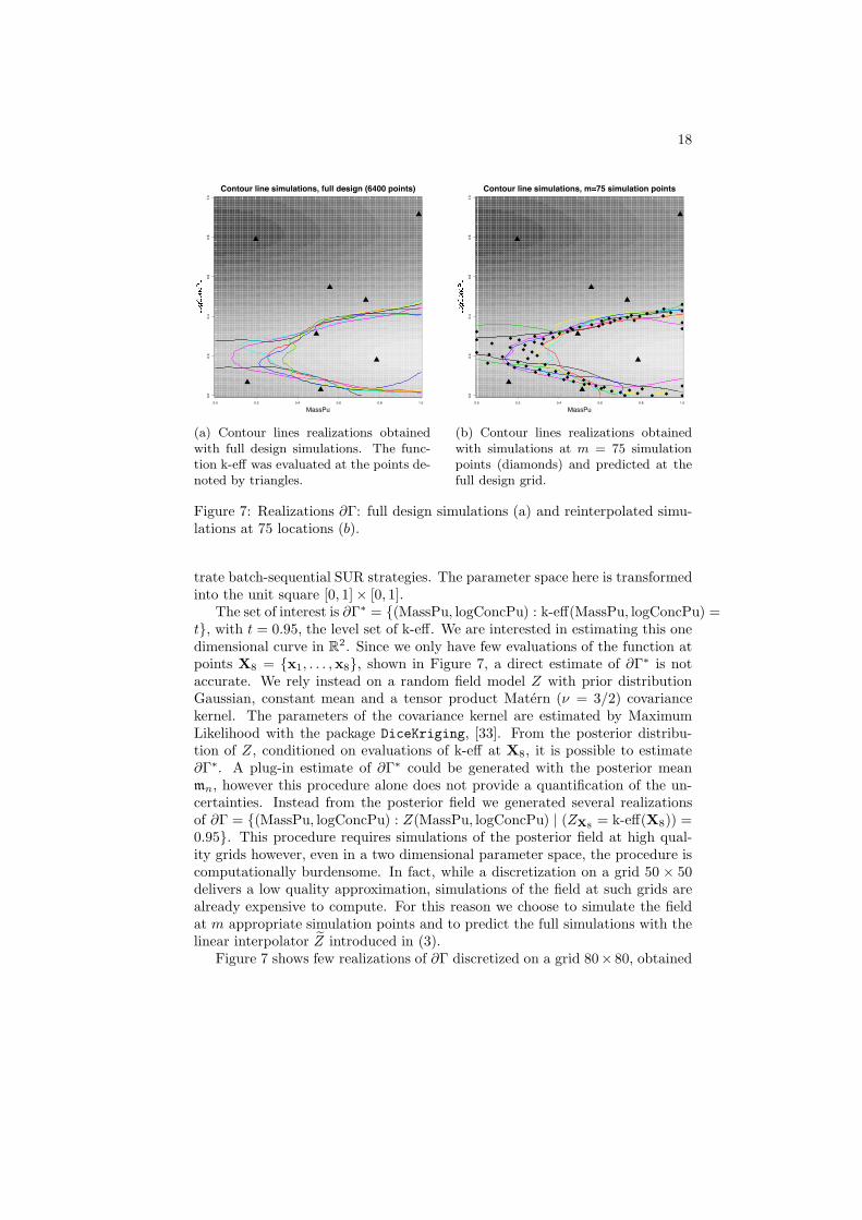
(a) Contour lines realizations obtainedwith full design simulations. The func-tion k-eff was evaluated at the points de-noted by triangles.

0.0 0.2 0.4 0.6 0.8 1.0

0.0

0.2

0.4

0.6

0.8

1.0

Contour line simulations, m=75 simulation points

MassPu

PQSTQUWXY

(b) Contour lines realizations obtainedwith simulations at m = 75 simulationpoints (diamonds) and predicted at thefull design grid.

Figure 7: Realizations ∂Γ: full design simulations (a) and reinterpolated simu-lations at 75 locations (b).

trate batch-sequential SUR strategies. The parameter space here is transformedinto the unit square [0, 1]× [0, 1].

The set of interest is ∂Γ∗ = {(MassPu, logConcPu) : k-eff(MassPu, logConcPu) =t}, with t = 0.95, the level set of k-eff. We are interested in estimating this onedimensional curve in R

2. Since we only have few evaluations of the function atpoints X8 = {x1, . . . ,x8}, shown in Figure 7, a direct estimate of ∂Γ∗ is notaccurate. We rely instead on a random field model Z with prior distributionGaussian, constant mean and a tensor product Matern (ν = 3/2) covariancekernel. The parameters of the covariance kernel are estimated by MaximumLikelihood with the package DiceKriging, [33]. From the posterior distribu-tion of Z, conditioned on evaluations of k-eff at X8, it is possible to estimate∂Γ∗. A plug-in estimate of ∂Γ∗ could be generated with the posterior meanmn, however this procedure alone does not provide a quantification of the un-certainties. Instead from the posterior field we generated several realizationsof ∂Γ = {(MassPu, logConcPu) : Z(MassPu, logConcPu) | (ZX8

= k-eff(X8)) =0.95}. This procedure requires simulations of the posterior field at high qual-ity grids however, even in a two dimensional parameter space, the procedure iscomputationally burdensome. In fact, while a discretization on a grid 50 × 50delivers a low quality approximation, simulations of the field at such grids arealready expensive to compute. For this reason we choose to simulate the fieldat m appropriate simulation points and to predict the full simulations with thelinear interpolator Z introduced in (3).

Figure 7 shows few realizations of ∂Γ discretized on a grid 80× 80, obtained

19

0.00

0.05

0.10

Z[\]

\Z ^] ]Z 75 100_`abcd ef gha`ijkhel mehlkg nao

KS

sta

tistics Threshold

pdhkhqji rji`c nsto

type

Algorithm B

Maximin LHS

KS statistics for H0u vwyzz{vm |}~~ ������������

Figure 8: Distributions of KS statistic computed over 100 experiments forKolmogorov-Smirnov test with null hypothesis H0 : Lfull = Lm. Simulationpoints chosen with Algorithm B or with maximin LHS design.

with simulations of the field at all points of the design (Figure 7a) and withsimulations at 75 simulation points, chosen with Algorithm B (Figure 7b). Thetwo sets of curves seem to share similar properties. The expected distance inmeasure between ∂Γ and ∂Γ, as introduced in Definition 1, could be used hereto quantify this similarity however, here we propose to use the arc length ofeach curve, defined as follows, as it is easier to interpret in our application.

Consider a regular grid G = {u1, . . . ,ur}. For each realization, we selectthe points G∂Γ = {u ∈ G : Zu | (ZX8

= k-eff(X8)) ∈ [0.95 − ε, 0.95 + ε]},where ε is small. G∂Γ contains all the points of the discrete design that haveresponse ε−close to the target. We order the points in G∂Γ in such a way that{ui1 , . . . ,uiJ } are vertices of a piecewise linear curve approximating ∂Γ. Weapproximate the arc length of the curve with the sum of the segments’ lengths:l(∂Γ) =

∑G∂Γ

‖uij−1− uij‖. By computing the length for each realization we

obtain a Monte Carlo estimate of the distribution of the arc length. We can nowcompare the distributions of arc length obtained from reconstructed realizationssimulated at few locations with the distribution obtained from simulations atthe full grid in order to select the number of simulation points that leads toquasi-realizations for ∂Γ whose length is indistinguishable from the full gridrealizations’ length.

Let us define the random variables Lfull = l(∂Γ6400) and Lm = l(∂Γm), thearc lengths of the random set generated with full design simulations (80 × 80grid) and the length of the random set generated with simulations at m pointsrespectively. We compare the distributions of Lfull and Lm with Kolmogorov-Smirnov tests for several values of m. The null hypothesis is H0 : Lfull = Lm.The distributions are approximated with 10, 000 simulations, either at the full

20

grid design or at the selected m points. For each m, 100 repetition of theexperiment were computed, thus obtaining a distribution for the Kolmogorov-Smirnov (KS) statistic. Figure 8 shows the value of the KS statistic for eachm, where the simulation points are obtained either with Algorithm B or with amaximin LHS design. For m ≥ 50 optimized points, the KS statistic is belowthe critical value for at least 97% of the experiments, thus it is not possibleto distinguish the two length distributions with a significance level of 5%. Ifthe simulation points are chosen with a maximin LHS design instead, the KSstatistic is below the critical value for at least 67% of the experiments with m =100 simulation points, as it is also shown in Figure 8. This result shows again theimportance of choosing optimized simulation points. The approximation of Lfull

with Lm leads to substantial computational time savings. The computationaltime for 10, 000 simulations of the field at the full grid design (6, 400 points) is466 seconds, while the total time for finding 75 appropriate simulation points(with Algorithm B), simulate the field at these locations and reinterpolate thefield at the full design is 48.7 seconds (average over 100 experiments).

The expected distance in measure introduced in Section 2.1 could also beused here to quantify how far the quasi-realizations are from the full grid real-izations.

7 Conclusions

In the context of excursion set estimation, simulating a conditional random fieldto obtain realizations of a related excursion set can be useful in many practicalsituations. Often, however, the random field needs to be simulated at a finedesign to obtain meaningful realizations of the excursion set. Even in moderatedimensions it is often impractical to simulate at such fine designs, thus renderinggood approximations hard to achieve.

In this paper we introduced a new method to simulate quasi-realizations ofa conditional Gaussian random field that mitigates this problem. While theapproach of predicting realizations of the field from simulations at few locationshas already been introduced in the literature, this is the first attempt to defineoptimal simulation points based on a specific distance between random closedsets: the expected distance in measure. We showed on several examples thatthe quasi-realizations method reduces the computational cost due to conditionalsimulations of the field, however it does so relying on an approximation. In par-ticular the random set quasi-realizations optimality with respect to the expecteddistance in measure does not necessarily guarantee that other properties of theset are correctly reproduced.

The quasi-realizations approach allowed us to study an uncertainty measurethat, to the best of our knowledge, was not previously used in practice: the dis-tance average variability. The estimation of the distance average variability isappealing when realizations of the excursion set on fine grids are computation-ally cheap. We showed on a two dimensional test function that it is possible toreduce computational costs by at least one order of magnitude, thus making this

21

technique practical. In general the quasi-realizations approach could improvethe speed of distance average based methods as, for example, [23] and [24].

We presented a test case in safety engineering where we estimated the arclength’s distribution of a level set in a two dimensional parameter space. Thelevel set was approximated by piecewise linear curve, the resolution of which de-pends on the simulation design. A Monte Carlo technique based on realizationsof the excursion set obtained with full design simulations is computationallytoo expensive at high resolutions. Reconstructed simulations from simulationsof the field at few well chosen points reinterpolated on a fine design made thisapplication possible. In particular we showed that the distribution of the arclength obtained with a full design simulation at a rough design, a grid 80 × 80,was not significantly different than the distribution obtained from reconstructedsets with simulations at m = 50 well chosen points, thus opening the way forestimates on higher resolution grids.

Conditional realizations of the excursion set can also be used to estimatethe volume of excursion, in appendix we show how to handle this problem withMonte Carlo simulations at fine designs.

We presented two algorithms to compute optimal simulation points. Whilethe heuristic Algorithm B is appealing for its computational cost and precision,there are a number of extensions that could lead to even more savings in com-putational time. For example, the optimization of the points in this work wascarried out with generic black box optimizers but it would be possible to achieveappreciable reductions in optimization time with methods based on analyticalgradients.

A Proof of Proposition 4

Let us first assume that s2n,m → 0 µ-almost everywhere. The expected dis-

tance in measure can be rewritten, according to Equation (4), as dµ,n(Γ, Γ) =∫Dρn,m(x)µ(dx). Since µ is a finite measure on D and ρn,m(x) ≤ 1, it is suffi-

cient by the dominated convergence theorem to prove that ρn,m → 0 µ-almosteverywhere.

Pick any x ∈ D such that s2n(x) > 0 and s2n,m(x) → 0. Then, for any w > 0,

ρn,m(x) ≤ Pn

(∣∣Z(x) − t∣∣ ≤ w

)+ Pn

(∣∣Z(x) − Z(x)∣∣ ≥ w

)

≤ 2w√2πs2n(x)

+s2n,m(x)

w2.

With w =√sn,m(x), it follows that

ρn,m(x) ≤ 2√sn,m(x)√2πs2n(x)

+ sn,m(x) → 0. (11)

Since s2n,m → 0 µ-almost everywhere and ρn,m(x) = 0 wherever s2n(x) = 0,Equation (11) proves the sufficiency part of Proposition 4.

22

Conversely, assume that dµ,n(Γ, Γ) → 0 when m → +∞, or equivalentlythat (ρn,m)m≥0 converges to zero in L1 (D,µ). Then (ρn,m)m≥0 also convergesto zero in measure:

∀ε > 0, µ(Aε

n,m

)−−−−−→m→+∞

0, where Aεn,m = {x ∈ D : ρn,m(x) ≥ ε}.

For any M > 1, consider the following sets:

Dn,M ={x ∈ D : 0 < 1

M sn(x) ≤∣∣t−mn(x)

∣∣ ≤ Msn(x)},

AM,εn,m = Dn,M ∩ Aε

n,m,

BM,εn,m = Dn,M ∩ {sn,m ≥ εsn} .

Then we have the following technical result.

Lemma 6. For all M > 1 and ε > 0, there exists ε′ > 0 (that does not dependon n, m or t) such that ∀x ∈ BM,ε

n,m, ρn,m(x) ≥ ε′, and therefore BM,εn,m ⊂ AM,ε′

n,m .

Using Lemma 6, for any M > 1 and ε > 0, we have

µ(BM,ε

n,m

)≤ µ

(AM,ε′

n,m

)≤ µ

(Aε′

n,m

)−−−−−→m→+∞

0.

In other words, (sn,m/sn)m≥0 converges to zero in measure on Dn,M . As a con-

sequence, since this is a decreasing sequence, (sn,m/sn)m≥0 converges to zero µ-almost everywhere on Dn,M , and therefore µ-almost everywhere on ∪M>1Dn,M ={x ∈ D : sn(x) > 0

}. Convergence also trivially holds where sn(x) = 0.

A.1 Proof of Lemma 6

Let M > 1, ε > 0, x ∈ BM,εn,m and set ζ = mn(x). Because BM,ε

n,m ⊂ Dn,M ,|t− ζ| ≥ ε sn(x) > 0 and in particular t 6= ζ. Assume, without loss of generality,that ζ < t and ε ≤ 1√

2. Recall that ρn,m(x) = Pn (En,m(x)) where En,m(x) is

the event defined by

En,m(x) ={x ∈ Γ∆Γ

}= E+

n,m(x) ∪ E−n,m(x),

E+n,m(x) =

{Z(x) < t, Z(x) ≥ t

},

E−n,m(x) =

{Z(x) ≥ t, Z(x) < t

}.

Recall also that, since Z is a Gaussian process, Z and ǫn,m(x) = Z(x) − Z(x)are independent Gaussian variables under Pn, with κ2

n,m(x) := Varn (ǫn,m(x)) =s2n(x) − s2n,m(x).

Let us first assume that sn,m(x) ≥ 1√2sn(x) ≥ εsn(x). As a consequence,

κn,m(x) ≤ 1√2sn(x) and therefore

t− ζ

κn,m(x)≥ 1

M

sn(x)

κn,m(x)≥

√2

Mand

t− ζ

sn,m(x)≤ M

sn(x)

sn,m(x)≤ M

√2.

23

For any w > 0, the following inclusions hold:

En,m(x) ⊃ E−n,m(x) =

{Z(x) < t and Z(x) + ǫn,m(x) ≥ t

}

⊃{ζ − w ≤ Z(x) ≤ t and ζ − w + ǫn,m(x) ≥ t

}

⊃{−w ≤ Z(x) − ζ ≤ t− ζ and ǫn,m(x) ≥ t− ζ + w

}.

With w = t− ζ, using the independence of Z(x) and ǫn,m(x), we get

ρn,m(x) ≥ Pn

(E−

n,m(x))

≥ Pn

(∣∣Z(x) − ζ∣∣ ≤ t− ζ

)Pn

(ǫn,m(x) ≥ 2(t− ζ)

)

≥(1 − 2Φ

(−√

2/M))

Φ(−2M

√2). (12)

Let us now assume that 1√2sn(x) ≥ sn,m(x) ≥ εsn(x). As a consequence,

κn,m(x) ≥ 1√2sn(x) and therefore

t− ζ

sn,m(x)≤ M

sn(x)

sn,m(x)≤ M

εand

1

M≤ t− ζ

κn,m(x)≤ M

√2.

For any w > 0, the following inclusions hold:

En,m(x) ⊃ E+n,m(x) =

{Z(x) ≥ t and Z(x) + ǫn,m(x) < t

}

⊃{t ≤ Z(x) ≤ t + w and ǫn,m(x) < −w

}.

Using again w = t− ζ and the independence of Z(x) and ǫn,m(x), we get

ρn,m(x) ≥ Pn

(E+

n,m(x))

≥ Pn

(t− ζ ≤ Z(x) − ζ ≤ 2(t− ζ)

)Pn

(ǫn,m(x) ≥ −(t− ζ)

)

≥ 1

Mϕ(2√

2M)

Φ

(−M

ε

), (13)

where ϕ denotes the probability density function of the standard Gaussian dis-tribution.

Finally, ρn,m(x) ≥ ε′, where ε′ denotes the minimum of the lower boundsobtained in (12) and (13).

B Application: Estimating the distribution of a

volume of excursion in six dimensions

In this section we show how it is possible to estimate the conditional distributionof the volume of excursion under a GRF prior by simulating at few well chosenpoints and predicting over fine designs.

24

In the framework developed in section 2, the random closed set Γ naturallydefines a distribution for the excursion set, thus µ(Γ) can be regarded as a ran-dom variable. In the specific case of a Gaussian prior, the expected volume ofexcursion can be computed analytically by integrating the coverage function,however here we use Monte Carlo simulations to work out the posterior distri-bution of this volume (see [40], [1]). In practice, a good estimation of the volumerequires a discretization of the random closed set on a fine design. However, al-ready in moderate dimensions (2 ≤ d ≤ 10), a discretization of the domain fineenough to achieve good approximations of the volume might require simulatingat a prohibitive number of points. Here we show how the proposed approachmitigates this problem on a six-dimensional example.

We consider the following test function h(x) = − log(−Hartman6(x)), whereHartman6 is the six-dimensional Hartman function (see [25]) defined on D =[0, 1]6 and we are interested in estimating the volume distribution of the excur-sion set Γ⋆ = {x ∈ D : h(x) ≥ t}, t = 6. The threshold t = 6 is chosen to obtaina true volume of excursion of around 3%, thus rendering the excursion region amoderately small set.

A GRF model is built with a Gaussian prior Z with a tensor product Materncovariance kernel (ν = 5/2). The parameters of the covariance kernel are es-timated by Maximum Likelihood from n = 60 observations of h; the sameobservations are used to compute the conditional random field. We considerthe discretization G = {u1, . . . ,ur} ⊂ D with r = 10, 000 and u1, . . . ,ur Sobol’points in [0, 1]6. The conditional field Z is simulated 10, 000 times on G andconsequently N = 10, 000 realizations of the trace of Γ over G are obtained.

The distribution of the volume of excursion can be estimated by comput-ing for each realization the proportion of points where the field takes valuesabove the threshold. While this procedure is acceptable for realizations comingfrom full design simulations, it introduces a bias when it is applied to quasi-realizations of the excursion set. In fact, the paths of the predicted field arealways smoother than the paths of full design simulations due to the linear na-ture of the predictor [36]. This introduces a systematic bias on the volume ofexcursion for each realization because subsets of the excursion sets induced bysmall rougher variations of the true Gaussian field may not be intercepted byZ. The effect changes the mean of the distribution, but it does not seem to in-fluence the variance of the distribution. In the present setting we observed thatthe mean volume of excursion was consistently underestimated. A modifica-tion of the classic estimate of the distribution of the volume is here considered.Given a discretization design G, of size r, the distribution of the volume ofexcursion is obtained with the following steps: first the mean volume of excur-sion is estimated by integrating the coverage function of Γ over G; second thedistribution is obtained by computing the volume of excursion for each quasi-realization of the excursion set; finally the distribution is centered in the meanvalue obtained with the first step. Figure 9a shows the absolute error on themean between the full design simulation and the approximate simulations withand without bias correction. The optimal simulation points are computed withAlgorithm B because for a large number of points it achieves very similar results

25

0.0

00

.02

0.0

40

.06

0.0

80

.10

������ �� ���������� ������ ���

����

m

�����

Fu

ll��

���

Fu

ll�

 ¡ ¢  £¡¡ £¤  £ ¡

Reconstructed realization

absolute error on the mean

¥��¦��� §��� ¨����¨����©������ª ���������

(a) Absolute error on the mean estimatebetween Vm and Vfull. The red line is theerror on the unbiased estimator, the blackline represents the error on the estimatorwithout bias correction.

0.0

20

.03

0.0

40

.05

0.0

60

.07

«¬­®¯° ±² ³´­¬µ¶·´±¸ ¹±´¸·³ º­»

¼½¾¿ÀÁÀ¿ÀÂÿ

50 75 ÄÅÅ ÄÆÇ ÄÇÅ

Kolmogorov�Smirnov statistics

ȹ·´­´É¯Ê ¹±´¸·³ ºË»Ì±®±µ ¹±´¸·³Í¯Î¯Ï·´±¸ 浬¯ ¶· ÅÑÅÇ

(b) Kolmogorov-Smirnov statistic for test-ing the hypothesis H0 : Vm = Vfull.Simulations at points obtained with Al-gorithm B (black full line) or with spacefilling points (blue dashed line). The dot-ted horizontal line is the rejection value atlevel 0.05.

Figure 9: Analysis of volume distributions.

to Algorithm A but at the same time the optimized points are much cheaper tocompute, as showed in the previous sections.

Denote with Vfull = µ(Γ(E10,000)) the random variable representing thevolume of the excursion set obtained with full design simulations and Vm =µ(Γ(Em)) the recentered random variable representing the volume of the recon-structed set obtained from simulations at m points. We compare the distributionof Vfull and Vm for different values of m with Kolmogorov-Smirnov two sam-ple tests. Figure 9b shows the values of the Kolmogorov-Smirnov statistic fortesting the null hypothesis H0 : Vm = Vfull, for m = 50, 75, 100, 125, 150. Vm

is computed both with simulation points optimized with Algorithm B and withpoints from a space filling Sobol’ sequence. The horizontal line is the rejectionvalue at level 0.05. With confidence level 0.05, the distribution of Vm is notdistinguishable from the distribution of Vfull if m ≥ 125 with optimized pointsand if m > 150 with Sobol’ points.

The estimate of the distribution of the volume of excursion is much fasterwith quasi-realizations from simulations at few optimal locations. In fact, thecomputational costs are significantly reduced with by interpolating simulations:the CPU time needed to simulate on the full 10, 000 points design is 60293 sec-onds while the total time for the optimization of m = 150 points, the simulationon those points and the prediction over the full design is 575 seconds. Bothtimes were computed on the cluster of the University of Bern with Intel Xeon

26

E5649 2.53GHz CPUs with 4GB RAM.

Acknowledgment

The authors wish to thank Ilya Molchanov for helpful discussions and YannRichet and Gregory Caplin (IRSN) for the challenging and insightful test case.The first author was supported by the Swiss National Science Foundation, grantnumber 200021 146354.

References

[1] R. J. Adler, On excursion sets, tube formulas and maxima of randomfields, Ann. Appl. Probab., 10 (2000), pp. 1–74.

[2] A. J. Baddeley and I. S. Molchanov, Averaging of random sets basedon their distance functions, J. Math. Imaging Vision, 8 (1998), pp. 79–92.

[3] M. J. Bayarri, J. O. Berger, E. S. Calder, K. Dalbey, S. Lu-

nagomez, A. K. Patra, E. B. Pitman, E. T. Spiller, and R. L.

Wolpert, Using statistical and computer models to quantify volcanic haz-ards, Technometrics, 51 (2009), pp. 402–413.

[4] J. Bect, D. Ginsbourger, L. Li, V. Picheny, and E. Vazquez, Se-quential design of computer experiments for the estimation of a probabilityof failure, Stat. Comput., 22 (3) (2012), pp. 773–793.

[5] M. Binois, D. Ginsbourger, and O. Roustant, Quantifying uncer-tainty on Pareto fronts with Gaussian process conditional simulations, Eu-ropean J. Oper. Res., 243 (2015), pp. 386–394.

[6] D. Bolin and F. Lindgren, Excursion and contour uncertainty regionsfor latent Gaussian models, Journal of the Royal Statistical Society: SeriesB (Statistical Methodology), (2014).

[7] P. Bratley and B. L. Fox, Algorithm 659: Implementing Sobol’s quasir-andom sequence generator, ACM Trans. Math. Software, 14 (1988), pp. 88–100.

[8] R. H. Byrd, P. Lu, J. Nocedal, and C. Zhu, A limited memory algo-rithm for bound constrained optimization, SIAM J. Sci. Comput., 16 (1995),pp. 1190–1208.

[9] C. Chevalier, J. Bect, D. Ginsbourger, E. Vazquez, V. Picheny,

and Y. Richet, Fast kriging-based stepwise uncertainty reduction with ap-plication to the identification of an excursion set, Technometrics, 56 (2014),pp. 455–465.

27

[10] C. Chevalier, D. Ginsbourger, J. Bect, and I. Molchanov, Esti-mating and quantifying uncertainties on level sets using the Vorob’ev ex-pectation and deviation with Gaussian process models, in mODa 10 Ad-vances in Model-Oriented Design and Analysis, D. Ucinski, A. Atkinson,and C. Patan, eds., Physica-Verlag HD, 2013.

[11] C. Chevalier, D. Ginsbourger, and X. Emery, Corrected kriging up-date formulae for batch-sequential data assimilation, in Mathematics ofPlanet Earth, Lecture Notes in Earth System Sciences, Springer BerlinHeidelberg, 2014, pp. 119–122.

[12] C. Chevalier, V. Picheny, and D. Ginsbourger, The KrigInv pack-age: An efficient and user-friendly R implementation of kriging-based in-version algorithms, Comput. Statist. Data Anal., 71 (2014), pp. 1021–1034.

[13] J.-P. Chiles and P. Delfiner, Geostatistics: Modeling Spatial Uncer-tainty, Second Edition, Wiley, New York, 2012.

[14] N. A. C. Cressie, Statistics for spatial data, Wiley, New York, 1993.

[15] A. Cuevas and R. Fraiman, Set estimation, in New Perspectives inStochastic Geometry, W. S. Kendall and I. Molchanov, eds., Oxford Univ.Press, Oxford, 2010, pp. 374–397.

[16] V. Dubourg, B. Sudret, and J.-M. Bourinet, Reliability-based de-sign optimization using kriging surrogates and subset simulation, Struct.Multidiscip. Optim., 44 (2011), pp. 673–690.

[17] P. Felzenszwalb and D. Huttenlocher, Distance transforms of sam-pled functions, tech. rep., Cornell University, 2004.

[18] J. P. French and S. R. Sain, Spatio-temporal exceedance locations andconfidence regions, Ann. Appl. Stat., 7 (2013), pp. 1421–1449.

[19] A. Genz, Numerical computation of multivariate normal probabilities, J.Comput. Graph. Statist., 1 (1992), pp. 141–149.

[20] R. B. Gramacy and H. K. H. Lee, Adaptive design and analysis ofsupercomputer experiments, Technometrics, 51 (2009), pp. 130–145.

[21] P. Hall and I. Molchanov, Sequential methods for design-adaptive es-timation of discontinuities in regression curves and surfaces, Ann. Statist.,31 (2003), pp. 921–941.

[22] M. Hamada, H. F. Martz, C. S. Reese, and A. G. Wilson, Findingnear-optimal bayesian experimental designs via genetic algorithms, Amer.Statist., 55 (2001), pp. 175–181.

[23] H. Jankowski and L. Stanberry, Expectations of random sets and theirboundaries using oriented distance functions, J. Math. Imaging Vision, 36(3) (2010), pp. 291–303.

28

[24] , Confidence regions for means of random sets using oriented distancefunctions, Scand. J. Stat., 39 (2) (2012), pp. 340–357.

[25] D. R. Jones, M. Schonlau, and W. J. Welch, Efficient global op-timization of expensive black-box functions, J. Global Optim., 13 (1998),pp. 455–492.

[26] C. Lantuejoul, Geostatistical simulation: models and algorithms,Springer, Berlin, 2002.

[27] W. R. J. Mebane and J. S. Sekhon, Genetic optimization using deriva-tives: The rgenoud package for R, Journal of Statistical Software, 42 (11)(2011), pp. 1–26.

[28] I. Molchanov, Theory of Random Sets, Springer, London, 2005.

[29] J. Oakley, Bayesian Uncertainty Analysis for Complex Computer Codes,PhD thesis, University of Sheffield, 1999.

[30] P. Ranjan, D. Bingham, and G. Michailidis, Sequential experimentdesign for contour estimation from complex computer codes, Technometrics,50 (2008), pp. 527–541.

[31] C. E. Rasmussen and C. K. I. Williams, Gaussian processes for ma-chine learning, MIT Press, 2006.

[32] M. Reitzner, E. Spodarev, D. Zaporozhets, et al., Set reconstruc-tion by Voronoi cells, Adv. in Appl. Probab., 44 (2012), pp. 938–953.

[33] O. Roustant, D. Ginsbourger, and Y. Deville, DiceKriging,DiceOptim: Two R packages for the analysis of computer experiments bykriging-based metamodelling and optimization, Journal of Statistical Soft-ware, 51 (2012), pp. 1–55.

[34] J. Sacks and S. Schiller, Spatial designs, Statistical decision theoryand related topics IV, 2 (1988), pp. 385–399.

[35] J. Sacks, W. J. Welch, T. J. Mitchell, and H. P. Wynn, Designand analysis of computer experiments, Statist. Sci., 4 (1989), pp. 409–435.

[36] M. Scheuerer, A comparison of models and methods for spatial inter-polation in statistics and numerical analysis, PhD thesis, University ofGottingen, 2009.

[37] M. L. Stein, Large sample properties of simulations using latin hypercubesampling, Technometrics, 29 (1987), pp. 143–151.

[38] , Interpolation of spatial data, some theory for kriging, Springer, NewYork, 1999.

29

[39] E. Vazquez and J. Bect, Convergence properties of the expected im-provement algorithm with fixed mean and covariance functions, J. Statist.Plann. Inference, 140:11 (2010), pp. 3088–3095.

[40] E. Vazquez and M. P. Martinez, Estimation of the volume of an ex-cursion set of a Gaussian process using intrinsic kriging, arXiv preprintmath/0611273, (2006).

[41] J. Villemonteix, E. Vazquez, and E. Walter, An informationalapproach to the global optimization of expensive-to-evaluate functions, J.Global Optim., 44 (2009), pp. 509–534.

[42] O. Y. Vorob’ev, Srednemernoje modelirovanie (mean-measure mod-elling), Nauka, Moscow, In Russian (1984).