quantification of facial asymmetry in children · quantification of facial asymmetry in children...
TRANSCRIPT
Quantification of Facial
Asymmetry in Children
Master´s Thesis, February 2012
IMM-M.Sc-2012-06
Yagmur Yücel

3
Quantification of Facial Asymmetry in Children
Author
Yagmur Yücel
Supervisors
Associate Professor Nuno V. Hermann
Department of Pediatric Dentistry and Clinical Genetics, School of
Dentistry, Faculty of Health Sciences, University of Copenhagen,
Copenhagen, Denmark
Research Engineer Tron A. Darvann
3D Craniofacial Image Research Laboratory (School of Dentistry,
University of Copenhagen; Copenhagen University Hospital; and DTU
Informatics, Technical University of Denmark), Copenhagen, Denmark
Professor Bjarne K. Ersbøll
DTU Informatics, Technical University of Denmark, Lyngby, Denmark
3D Craniofacial Image Research Laboratory
(School of Dentistry, University of Copenhagen;
Copenhagen University Hospital; and
DTU Informatics, Technical University of Denmark),
Copenhagen, Denmark
Release date: February 2012
Edition: 1. Edition
Comments: This report is a part of the requirements to achieve Master of
Science in Engineering (MSc) at Technical University of
Denmark and University of Copenhagen.
The report represents 30 ECTS points.
Rights: © Yagmur Yücel, 2012

4

5
Preface
The purpose of this Master Thesis is to estimate the average facial asymmetry and its
variation in normal children.
This project was carried out during a time period of approximately 6-months at the 3D
Craniofacial Image Research Laboratory, University of Copenhagen, Copenhagen,
Denmark, and DTU Informatics, Technical University of Denmark, Lyngby, Denmark.
The report presents the results of asymmetry quantification, implementations and
conclusions. The methods, ideas and analysis are described to a level of detail, making
it possible to understand, reconstruct and further build the methods and results of this
Thesis.

6

7
Acknowledgements
First of all I will thank my family for their support and for their backing. Thanks for
believing in me and for your understanding throughout my whole project time.
Thanks to my main supervisor at 3D laboratory Nuno V. Hermann for her help and
useful suggestions during the project.
Special thanks to my co-supervisor Tron A. Darvann for his support and valuable help
throughout the whole project time. Grateful thanks for your time and kindness.
Thanks to my DTU supervisor Bjarne K. Ersbøll for his valued suggestions at our
meetings.
It was a pleasure to meet you Peter Larsen, and thanks for your technical support,
participation in our meetings and for your cake breaks.
Thanks to Rasmus Larsen and Knut Conradsen for your suggestions and interest during
our Friday meetings.
Finally thanks to Alex Kane and Angelo Lipira for most of the data used in this project.

8

9
Abstract
This study is about quantifying the average asymmetry and how it varies in faces of
normal children of different ages, gender and ethnicity. The overall purpose is to be
able to answer questions like the following:
How asymmetrical are human faces?
Do people become more asymmetrical with age?
Is the asymmetry and its variation different in different populations?
Is asymmetry different in girls and boys?
Are there particular regions in the face that are more asymmetrical than
others?
What are the typical patterns of variation of facial asymmetry?
What is the origin of facial asymmetry?
Can asymmetry quantification be used as a diagnostic tool; i.e. can it discern
between different phenotypes of facial malformations?
Can asymmetry be used as a tool for quantification of the severity of a
particular disorder, and thereby be used in the context of treatment
progression and evaluation?
Motivations for studying asymmetry are thus either biological (top seven questions
above) or clinical (bottom two questions above), although the biological questions are
also relevant in a clinical setting: improved knowledge of the biological aspects of
asymmetry is important in making the best choices in relation to treatment.
Many craniofacial anomalies are characterized by distinct patterns of asymmetry, and
often the goal of surgery is to reduce and normalize the amount of asymmetry. For this

10
kind of treatment, the surgeons need a reference quantifying how asymmetric people
normally are. For this purpose, it could be useful to have a database of asymmetry of
normal faces. By a normal individual, we mean an individual who has had no history of
craniofacial disease or trauma.
The goal of the present work is to develop methodology for quantification of facial
asymmetry and apply it to human populations in order to answer the above questions.
In particular, the thesis is concerned with quantifying asymmetry in a large population
(n = 375) of normal children, thus providing reference values that can be used e.g. for
treatment purposes. The thesis thus develops and presents a normative “database” of
asymmetry.
Asymmetry is defined as the geometrical difference between the left and right side of
the face. Quantification of asymmetry thus involves 1) determination of the dividing
plane (midsagittal plane) between the left and right side of the face (this is achieved by
use of rigid registration and 2) determination of corresponding anatomical locations on
the left and right side, which is achieved either by a) direct manual landmarking, b)
landmark-guided non-rigid registration of a symmetric template, or c) automatic non-
rigid registration of a face surface to its mirror-surface.
The two landmark-based methods were found to perform well, providing asymmetry
estimates at a sparse set of landmark positions, or spatially densely across the entire
face, respectively. The automatic, surface based method was seen to have low
sensitivity: it was not able to detect sufficiently small amounts of asymmetry to be
reliably used in normal faces.
After testing all three methods on smaller subsamples of surface scans of normal
children available in the Craniobank database, a larger study of asymmetry, including
11
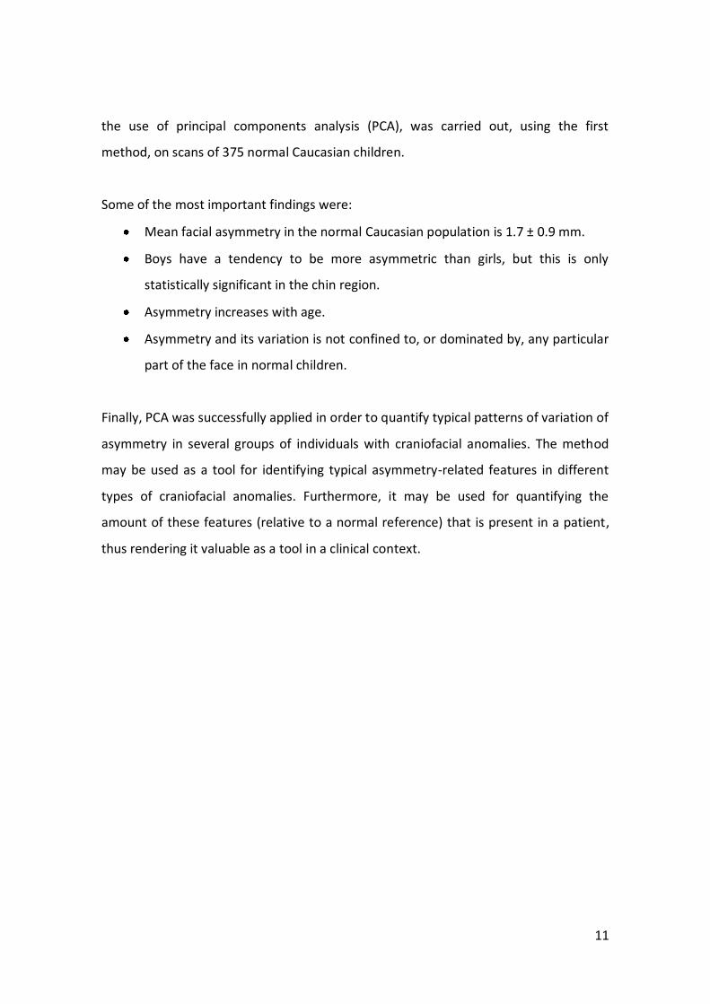
the use of principal components analysis (PCA), was carried out, using the first
method, on scans of 375 normal Caucasian children.
Some of the most important findings were:
Mean facial asymmetry in the normal Caucasian population is 1.7 ± 0.9 mm.
Boys have a tendency to be more asymmetric than girls, but this is only
statistically significant in the chin region.
Asymmetry increases with age.
Asymmetry and its variation is not confined to, or dominated by, any particular
part of the face in normal children.
Finally, PCA was successfully applied in order to quantify typical patterns of variation of
asymmetry in several groups of individuals with craniofacial anomalies. The method
may be used as a tool for identifying typical asymmetry-related features in different
types of craniofacial anomalies. Furthermore, it may be used for quantifying the
amount of these features (relative to a normal reference) that is present in a patient,
thus rendering it valuable as a tool in a clinical context.

12
13
Contents
PREFACE ..................................................................................................................................... 5
ACKNOWLEDGEMENTS ................................................................................................................... 7
ABSTRACT ................................................................................................................................... 9
CHAPTER 1.............................................................................................................................. 21
INTRODUCTION .......................................................................................................................... 21
1.1 MOTIVATION ........................................................................................................................ 21
1.2 CRANIOFACIAL ANOMALIES ...................................................................................................... 22
1.3 TREATMENT ......................................................................................................................... 25
1.4 PURPOSE OF THE PROJECT ....................................................................................................... 26
1.5 PREVIOUS WORK ................................................................................................................... 28
1.6 THESIS STRUCTURE ................................................................................................................. 30
CHAPTER 2.............................................................................................................................. 33
MATERIAL ................................................................................................................................. 33
2.1 DATA .................................................................................................................................. 33
2.2 ACQUISITION AND FORMATS .................................................................................................... 35
CHAPTER 3.............................................................................................................................. 37
ASYMMETRY .............................................................................................................................. 37
3.1 DEFINITION OF ASYMMETRY ..................................................................................................... 37
3.2 FLUCTUATING ASYMMETRY ...................................................................................................... 40
3.3 DIRECTIONAL ASYMMETRY ...................................................................................................... 40
CHAPTER 4.............................................................................................................................. 41
14
SHAPE ANALYSIS ........................................................................................................................ 41
4.1 SHAPE ................................................................................................................................. 41
4.2 TEMPLATE ............................................................................................................................ 41
4.3 LANDMARKS ......................................................................................................................... 42
4.4 ESTABLISHMENT OF DETAILED POINT CORRESPONDENCE ................................................................. 44
4.5 SURFACE TRANSFORMATION .................................................................................................... 44
4.6 RIGID/NON-RIGID REGISTRATION............................................................................................... 46
4.7 THIN-PLATE SPLINES .............................................................................................................. 47
4.8 B-SPLINES ............................................................................................................................ 48
4.9 PRINCIPAL COMPONENTS ANALYSIS ............................................................................................ 49
CHAPTER 5.............................................................................................................................. 51
QUANTIFICATION OF FACIAL ASYMMETRY AT MANUALLY PLACED LANDMARK LOCATIONS .......................... 51
5.1 INTRODUCTION ..................................................................................................................... 51
5.2 MATERIAL ............................................................................................................................ 52
5.3 METHOD ............................................................................................................................. 52
5.3.1 Computation of asymmetry ............................................................................................ 53
5.3.2 Implementation ............................................................................................................. 58
5.3.3 Error due to manual landmarking ................................................................................... 58
5.4 RESULTS .............................................................................................................................. 58
5.4.1 Asymmetry computation ................................................................................................ 59
5.4.2 Asymmetry quantification using the landmarks from second placement ........................ 65
5.4.3 Comparison of first and second landmarking results ...................................................... 67
5.5 DISCUSSION AND CONCLUSION ................................................................................................. 72
CHAPTER 6.............................................................................................................................. 73
SPATIALLY DETAILED QUANTIFICATION OF FACIAL ASYMMETRY USING MANUALLY PLACED LANDMARKS ........ 73
6.1 INTRODUCTION ..................................................................................................................... 73
6.2 MATERIAL ............................................................................................................................ 74
6.3 METHOD ............................................................................................................................. 75
6.3.1 Creation of a symmetric template .................................................................................. 76

15
6.3.2 Landmarking .................................................................................................................. 78
6.3.3 Orient............................................................................................................................. 79
6.3.4 Match ............................................................................................................................ 79
6.3.5 Asy ................................................................................................................................. 80
6.4 RESULTS .............................................................................................................................. 81
6.4.1 Quantification of asymmetry using 26 landmarks ........................................................... 81
6.4.2 Comparison of results using 6 vs. 19 landmarks .............................................................. 89
6.4.3 Validation ....................................................................................................................... 91
6.4.4 Comparison between the method presented in the current chapter and the method of
Chapter 5 ................................................................................................................................ 92
6.5 DISCUSSION AND CONCLUSION ................................................................................................. 95
6.5.1 Asymmetry in 10 African American boys......................................................................... 95
6.5.2 Landmarking by looking at one side of the face and at the whole face ............................ 95
6.5.3 The importance of position of landmarks ....................................................................... 96
6.5.4 The importance of number of landmarks ........................................................................ 96
6.5.5 Validation: The symmetric and wide face ....................................................................... 97
6.5.6 Validation of landmark based method ............................................................................ 99
CHAPTER 7............................................................................................................................ 101
AUTOMATIC QUANTIFICATION OF FACIAL ASYMMETRY USING NON-RIGID SURFACE REGISTRATION ............ 101
7.1 INTRODUCTION ................................................................................................................... 101
7.2 MATERIAL .......................................................................................................................... 102
7.3 METHOD ........................................................................................................................... 102
7.3.1 Orientation................................................................................................................... 104
7.3.2 Flipping ........................................................................................................................ 105
7.3.3 Deformation/matching ................................................................................................. 106
7.3.4 Difference .................................................................................................................... 107
7.4 RESULTS ............................................................................................................................ 109
7.4.1 Asymmetry quantification ............................................................................................ 109
7.4.2 Comparison between surface and landmark based method.......................................... 113
7.5 DISCUSSION AND CONCLUSION ............................................................................................... 116
16
7.5.1 Asymmetry quantification ............................................................................................ 116
7.5.2 Validation ..................................................................................................................... 117
CHAPTER 8............................................................................................................................ 121
FACIAL ASYMMETRY IN A LARGER GROUP OF NORMAL CHILDREN ........................................................ 121
8.1 INTRODUCTION ................................................................................................................... 121
8.2 MATERIAL .......................................................................................................................... 122
8.3 METHOD ........................................................................................................................... 122
8.3.1 Asymmetry quantification ............................................................................................ 123
8.3.2 Implementation of principal components analysis (PCA) .............................................. 126
8.4 RESULTS ............................................................................................................................ 127
8.4.1 Asymmetry quantification ............................................................................................ 128
8.4.2 Comparison between boys and girls and asymmetry vs. age ......................................... 131
8.4.3 Principal Components Analysis (PCA) ............................................................................ 134
8.4.3.1 Principal Component Modes for the asymmetry ........................................................ 134
8.4.3.2 Principal Component Modes for the x-axis of asymmetry .......................................... 139
8.4.3.3 Principal Component Modes for the y-axis of asymmetry .......................................... 142
8.4.3.4 Principal Component Modes for the z-axis of asymmetry .......................................... 145
8.4.3.5 Principal Component Score plots ............................................................................... 148
8.4.3.6 Principal Component Score plots for boys vs. girls ..................................................... 149
8.4.3.7 Total variance percentage ......................................................................................... 150
8.5 DISCUSSION........................................................................................................................ 150
8.5.1 Asymmetry for the faces and landmark locations ......................................................... 150
8.5.3 Asymmetry relation for boys and girls and asymmetry vs. age ...................................... 153
8.5.4 PCA .............................................................................................................................. 154
8.6 CONCLUSION ...................................................................................................................... 158
CHAPTER 9............................................................................................................................ 159
PRINCIPAL COMPONENTS ANALYSIS FOR QUANTIFICATION OF DIFFERENCES IN ASYMMETRY BETWEEN
DIFFERENT TYPES OF CRANIOFACIAL ANOMALIES AND NORMAL POPULATION ........................................ 159
9.1 INTRODUCTION ................................................................................................................... 159

17
9.2 MATERIAL .......................................................................................................................... 159
9.3 METHOD ........................................................................................................................... 160
9.4 RESULTS ............................................................................................................................ 160
9.4.1 Asymmetry quantification ............................................................................................ 160
9.4.2 Principal Component Analysis....................................................................................... 165
9.4.2.1 Principal Component Score plots ............................................................................... 165
9.4.2.2 Principal Component mode plots ............................................................................... 168
9.5 DISCUSSION........................................................................................................................ 170
9.5.1 Asymmetry quantification ............................................................................................ 170
9.5.2 Score and mode plots ................................................................................................... 171
9.6 CONCLUSION ...................................................................................................................... 171
CHAPTER 10 .......................................................................................................................... 173
CONCLUSION ........................................................................................................................... 173
BIBLIOGRAPHY ..................................................................................................................... 175
APPENDIX A.1 ....................................................................................................................... 179
COMPARISON BETWEEN METHOD PRESENTED IN CHAPTER 5 AND 6...................................................... 179
APPENDIX A.2 ....................................................................................................................... 183
COMPARISON BETWEEN METHOD PRESENTED IN CHAPTER 6 AND 7...................................................... 183
APPENDIX B.1 ....................................................................................................................... 187
PCA ....................................................................................................................................... 187
APPENDIX C.1 ....................................................................................................................... 191
MATLAB SCRIPTS ...................................................................................................................... 191
READ FILES............................................................................................................................... 191

18
LOAD FILES .............................................................................................................................. 193
CENTROID SIZE.......................................................................................................................... 194
ASYMMETRY QUANTIFICATION ..................................................................................................... 195
Landmark based method ...................................................................................................... 195
Face Analyzer ........................................................................................................................ 207
Surface based method .......................................................................................................... 208
PRINCIPAL COMPONENT ANALYSIS ................................................................................................ 209
MODE PLOTS ............................................................................................................................ 213
PCA FOR CHILDREN WITH NORMAL AND ABNORMAL FACES ................................................................ 228
HISTOGRAM OF AGE FOR THE CHILDREN ......................................................................................... 242
APPENDIX D.1....................................................................................................................... 243
LANDMARKER SCRIPT ................................................................................................................ 243
FLIP MANY SURFACES ................................................................................................................. 243
SNREG MANY SURFACES (DEFORMATION) ....................................................................................... 244
DIFFERENCE MANY SURFACES ....................................................................................................... 245
APPENDIX E.1 ....................................................................................................................... 251
PROJECT DESCRIPTION ............................................................................................................... 251
PROJECT TITLE .......................................................................................................................... 251
THESIS STATEMENT .................................................................................................................... 251
PURPOSE ................................................................................................................................. 251
ASYMMETRY ............................................................................................................................ 252
METHOD ................................................................................................................................. 252
VALIDATION ............................................................................................................................. 253
STATISTICAL ANALYSIS ................................................................................................................ 253
OVERALL PROJECT PLAN .............................................................................................................. 254
GANTT DIAGRAM .................................................................................................................. 255
APPENDIX E.2 ....................................................................................................................... 256

19
LEARNING OBJECTIVES ............................................................................................................... 256

20

Chapter 1
21
Chapter 1
Introduction
1.1 Motivation
Imagine living with a very asymmetrical face! A face that other people stare at when
they look at you.
This is in fact how many people in the world are living.
For a human being, it is important to be self-confident and to like the way you look. If
not, it may affect your whole life style and have an emotional impact which can lead to
e.g. depression.
Craniofacial anomalies (CFA) are disorders that in many cases affect the appearance. In
addition, the abnormal appearance may be one of the manifestations of a possible life-
threatening condition that needs to be treated. Some of these people have the
opportunity to get treated. Through surgical treatment, functional abilities, as well as
appearance are sought to be normalized. For this kind of treatment, the surgeons and
other members of the team of medical and dental professionals need a reference
quantifying how people normally look. For this purpose it could be useful to have a
database of asymmetry of normal faces because people are not only asymmetric in
disease, but also in the normal population. The database could consist of information
about the amount and location of asymmetry in normal children. By a normal
individual, we mean an individual who has had no history of craniofacial disease or

Chapter 1
22
trauma. Such a database could also be expected to be of paramount importance in
studies of the etiology (reasons why). It is important to know how much asymmetry is
connected with genetics, environmental factors, growth, sutures etc.
The goal of this Thesis is to estimate the average facial asymmetry and its variation in
populations of normal children, in order to build such a database.
1.2 Craniofacial anomalies
Craniofacial anomalies are a varied group of deformities in the growth of the head and
the facial bones. The anomalies can be divided into two groups: those that are
congenital (present at birth) and those that are acquired later in life. The acquired
deformities can be caused by external factors like for instance pressure on the skull
due to a tumor.
The normal skull consists of many plates of bones that are separated by sutures
(growth zones or fibrous joints). The sutures are places between the bones in the
head. The sutures close and form an almost solid piece of bone (the skull) at the time
when the growth of the head has been completed.
Chapter 1
23
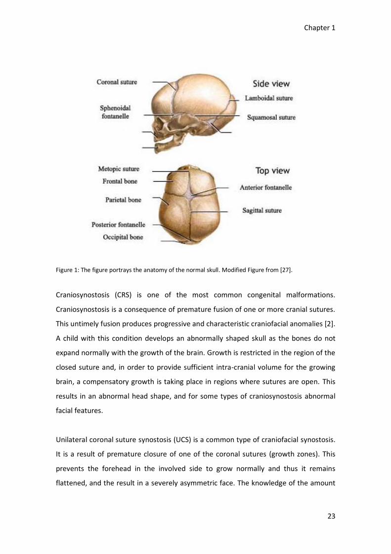
Figure 1: The figure portrays the anatomy of the normal skull. Modified Figure from [27].
Craniosynostosis (CRS) is one of the most common congenital malformations.
Craniosynostosis is a consequence of premature fusion of one or more cranial sutures.
This untimely fusion produces progressive and characteristic craniofacial anomalies [2].
A child with this condition develops an abnormally shaped skull as the bones do not
expand normally with the growth of the brain. Growth is restricted in the region of the
closed suture and, in order to provide sufficient intra-cranial volume for the growing
brain, a compensatory growth is taking place in regions where sutures are open. This
results in an abnormal head shape, and for some types of craniosynostosis abnormal
facial features.
Unilateral coronal suture synostosis (UCS) is a common type of craniofacial synostosis.
It is a result of premature closure of one of the coronal sutures (growth zones). This
prevents the forehead in the involved side to grow normally and thus it remains
flattened, and the result in a severely asymmetric face. The knowledge of the amount

Chapter 1
24
and location of asymmetry in a face is vital in order to diagnose and treat anomalies of
the face [30].
Figure 2: A schematic presentation of sutures and the skull deformities resulting from synostosis [28].
Cleft lip (split of the upper lip) and cleft palate (split of the roof of the mouth) is the
most common type of congenital facial malformation. This type of craniofacial
anomaly occurs if the tissue that forms the roof of the mouth and upper lip do not join
early in pregnancy. Apart from the fact that it can affect the child´s facial appearance,
it can also lead to problems with eating and talking.
Another type of facial deformation that affects children is juvenile idiopathic arthritis
(JIA). JIA is a chronic disease that can affect joints in any part of the body. The immune
system attacks the synovium (the tissue inside the joint) which leads to that the
synovium makes excess fluid (synovial fluid) that leads to swelling, pain and stiffness.
Without treatment, the synovium and inflammation process can spread to the
surrounding tissue which can induce damage on the cartilage and bone [35].
Chapter 1
25
Craniofacial anomalies are thought to have many different causes and it is an active
area of current research. Genetics and environmental factors are important issues, but
the exact causes are in many cases unknown [11].
1.3 Treatment
Surgery is usually the preferred treatment for craniofacial anomalies regardless of
whether they are congenital or acquired. For both types of anomalies, the purpose of
the treatment can be to reduce the pressure in the head and correct the deformities of
the face and the skull bone. The preference is that the face becomes as symmetric as
possible. The surgery usually takes place before the child is one year of age, since the
timing in relation to progression of deformity is best and the bones are still soft during
that period.
Often, maxillofacial surgery is needed for the treatment of many acquired craniofacial
anomalies. This type of surgery is carried out in the facial regions of the mouth and
jaws. Acquired craniofacial anomalies may be caused by e.g. cancer, trauma or arthritis
and many others. The damaged tissue can be removed and the face can be rebuilt by
this surgery. Also, plastic surgery can be applied to patients with cleft lip and palate
(Figure 3).

Chapter 1
26
Figure 3: Before and after surgery pictures of child with unilateral cleft lip and palate. Modified from
[33] and [34].
1.4 Purpose of the project
The purpose of this project is to estimate the average facial asymmetry and its
variation in different populations of normal children. The overall purpose is to be able
to answer questions like the following:
How asymmetrical are human faces?
Do people become more asymmetrical with age?
Is the asymmetry and its variation different in different populations?
Is asymmetry different in girls and boys?
Are there particular regions in the face that are more asymmetrical than
others?
What are the typical patterns of variation of facial asymmetry?
What is the origin of facial asymmetry?

Chapter 1
27
Can asymmetry quantification be used as a diagnostic tool; i.e. can it discern
between different phenotypes of facial malformations?
Can asymmetry be used as a tool for quantification of the severity of a
particular disorder, and thereby be used in the context of treatment
progression and evaluation?
Motivations for studying asymmetry are thus either biological (top seven questions
above) or clinical (bottom two questions), although the biological questions are also
relevant in a clinical setting: improved knowledge of the biological aspects of
asymmetry is important in making the best choices in relation to treatment.
Many craniofacial anomalies are characterized by distinct patterns of asymmetry, and
often the goal of surgery is to reduce and normalize the amount of asymmetry. For this
kind of treatment, the surgeons need a reference quantifying how asymmetric people
normally are. Therefore it could be useful to have a database of asymmetry of normal
faces. By a normal individual, we mean an individual who has had no history of
craniofacial disease or trauma.
The goal of the present work is to develop methodology for quantification of facial
asymmetry and apply it to human populations in order to answer the above questions.
Chapter 1
28
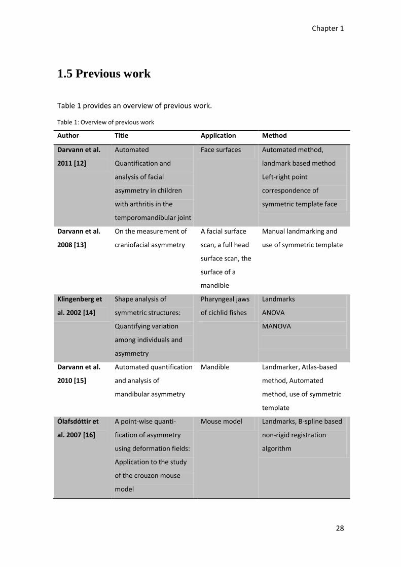
1.5 Previous work
Table 1 provides an overview of previous work.
Table 1: Overview of previous work
Author Title Application Method
Darvann et al.
2011 [12]
Automated
Quantification and
analysis of facial
asymmetry in children
with arthritis in the
temporomandibular joint
Face surfaces Automated method,
landmark based method
Left-right point
correspondence of
symmetric template face
Darvann et al.
2008 [13]
On the measurement of
craniofacial asymmetry
A facial surface
scan, a full head
surface scan, the
surface of a
mandible
Manual landmarking and
use of symmetric template
Klingenberg et
al. 2002 [14]
Shape analysis of
symmetric structures:
Quantifying variation
among individuals and
asymmetry
Pharyngeal jaws
of cichlid fishes
Landmarks
ANOVA
MANOVA
Darvann et al.
2010 [15]
Automated quantification
and analysis of
mandibular asymmetry
Mandible Landmarker, Atlas-based
method, Automated
method, use of symmetric
template
Ólafsdóttir et
al. 2007 [16]
A point-wise quanti-
fication of asymmetry
using deformation fields:
Application to the study
of the crouzon mouse
model
Mouse model Landmarks, B-spline based
non-rigid registration
algorithm

Chapter 1
29
Demant et al.
2010 [23]
3D analysis of facial
asymmetry in subjects
with juvenile idiopathic
arthritis (JIA)
Face surfaces
with a view to JIA
Landmarks
Lanche et al.
2007 [24]
A statistical model of
head asymmetry in
infants with
deformational
plagiocephaly
Head surfaces Detailed point
correspondence between
surfaces points on left and
right side of the head
Lipira et al.
2010 [25]
Helmet versus active
repositioning for
plagiocephaly: A three-
dimensional analysis
Whole head
surfaces
Detailed right-to-left point
correspondence between
head surfaces
Quantification of facial and craniofacial asymmetry is an active area of current
research. Facial asymmetry has been quantified using different methods. For instance,
an automatic method has been used and then validated by comparison to a landmark
based method of asymmetry quantification, and the two methods seemed to show
similar results [12]. Other scientists used different methods which showed
advantage/disadvantages depending on the application [13]. In another article [14] the
authors analyzed the shape variation in structures with object symmetry. After
landmarking the shape, the landmarks were mirrored across a midsagittal plane and
subsequently an average of the original and mirrored shapes were found, representing
a fully symmetric shape (Figure 4), before analysis was carried out.

Chapter 1
30
Figure 4: The figure to the left is from the article [14]. It is a schematic drawing showing a set of
landmarks, the mirrored landmarks and the average of both. The right figure shows the landmarks and
the mirrored landmarks for one of the normal faces studied in the present work. The landmarks are:
right/left ear, right/left eyebrow, right/left eye outer corner, right/left nose, right/left mouth corner,
nasion and chin.
Generally, the studies have been performed on abnormal faces or heads in humans or
animal models. On the contrary, the present study will be conducted on normal human
faces, since the aim of this Thesis is to estimate the asymmetry for normal faces which
can be later used in connection with diagnostics and treatment of abnormal faces
(Chapter 9).
1.6 Thesis structure
In the first part of the current Thesis, the material used in the study is presented. Then
a description and definition of asymmetry is given in Chapter 3. Subsequently, a
Chapter 1
31
description of the analysis of shapes is described (Chapter 4) to understand the
subsequent chapters about shape analysis.
In Chapters 5, 6 and 7 three different methods of asymmetry quantification is
developed and presented. Figure 5 classifies the three methods along the axes of a 3D
cube.
In Chapter 5 an asymmetry measure is defined and used in order to estimate the facial
asymmetry in a sparse set of manually placed landmark locations.
In Chapter 6, asymmetry is quantified at every spatial point location across the facial
surface scan. We term this spatially detailed quantification of asymmetry as opposed
to the spatially sparse asymmetry determined only at landmark locations. The method
used in both chapters is the landmark based method also called manual or guided
method.
Chapter 7 quantifies asymmetry at every spatial point location across the facial surface
scan as the method presented in Chapter 6. In Chapter 7, the surface based method
also called the automatic method (see Figure 5 for schematic illustration of the used
methods in the present Thesis) is used.
In Chapter 8, the method presented in Chapter 5 is used to quantify facial asymmetry
in surface scans of a larger group of normal children. A framework for applying
principal components analysis (PCA) is developed, implemented and applied to normal
children to provide information about the dominant types of variation in the data.
Subsequently, in Chapter 9, the framework for applying PCA is further applied for
quantification of the most important differences in asymmetry between different
types of craniofacial anomalies.

Chapter 1
32
Finally, Chapter 10 provides a conclusion, pointing out the most important results of
the present Thesis.
Figure 5: Classification of the methods developed and applied in the different chapters in the Thesis.
The methods are classified along three axes of a 3D cube. X-axis (red): the amount of automation of the
method; Y-axis (green): amount of spatial detail of asymmetry quantification; Z-axis (blue): type of
feature used for establishment of left-right correspondence. The location of the methods used in the
different chapters along the axes of the cube is indicated by the cyan balls.
Chapter 2
33
Chapter 2
Material
2.1 Data
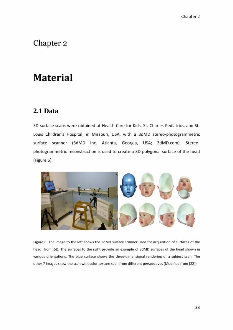
3D surface scans were obtained at Health Care for Kids, St. Charles Pediatrics, and St.
Louis Children's Hospital, in Missouri, USA, with a 3dMD stereo-photogrammetric
surface scanner (3dMD Inc. Atlanta, Georgia, USA; 3dMD.com). Stereo-
photogrammetric reconstruction is used to create a 3D polygonal surface of the head
(Figure 6).
Figure 6: The image to the left shows the 3dMD surface scanner used for acquisition of surfaces of the
head (from [5]). The surfaces to the right provide an example of 3dMD surfaces of the head shown in
various orientations. The blue surface shows the three-dimensional rendering of a subject scan. The
other 7 images show the scan with color texture seen from different perspectives (Modified from [22]).
Chapter 2
34
The surface scans of faces used in the present Thesis have been selected from
“Craniobank” which is a collection of surface scans of the head and face in
approximately 1300 normal children ranging in age from infants to age 18 years and of
various ethnic backgrounds. It was created by pediatric plastic and reconstructive
surgeons and students at Washington University School of Medicine in St. Louis, in
Missouri, USA. Craniobank is the first free and searchable online database that helps
researchers study the normal form and growth of the head and face [22].
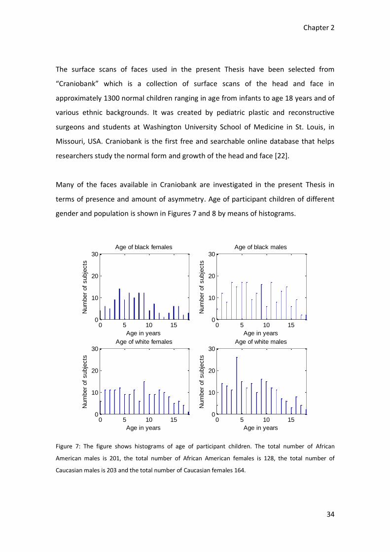
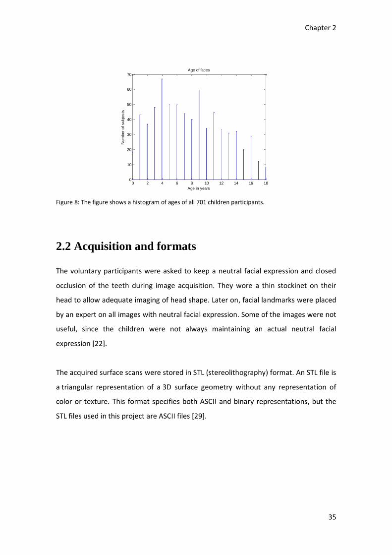
Many of the faces available in Craniobank are investigated in the present Thesis in
terms of presence and amount of asymmetry. Age of participant children of different
gender and population is shown in Figures 7 and 8 by means of histograms.
Figure 7: The figure shows histograms of age of participant children. The total number of African
American males is 201, the total number of African American females is 128, the total number of
Caucasian males is 203 and the total number of Caucasian females 164.
0 5 10 150
10
20
30
Age in years
Num
ber
of
subje
cts
Age of black females
0 5 10 150
10
20
30
Age in years
Num
ber
of
subje
cts
Age of black males
0 5 10 150
10
20
30
Age in years
Num
ber
of
subje
cts
Age of white females
0 5 10 150
10
20
30
Age in years
Num
ber
of
subje
cts
Age of white males
Chapter 2
35
Figure 8: The figure shows a histogram of ages of all 701 children participants.
2.2 Acquisition and formats
The voluntary participants were asked to keep a neutral facial expression and closed
occlusion of the teeth during image acquisition. They wore a thin stockinet on their
head to allow adequate imaging of head shape. Later on, facial landmarks were placed
by an expert on all images with neutral facial expression. Some of the images were not
useful, since the children were not always maintaining an actual neutral facial
expression [22].
The acquired surface scans were stored in STL (stereolithography) format. An STL file is
a triangular representation of a 3D surface geometry without any representation of
color or texture. This format specifies both ASCII and binary representations, but the
STL files used in this project are ASCII files [29].
0 2 4 6 8 10 12 14 16 180
10
20
30
40
50
60
70
Age in years
Num
ber
of
subje
cts
Age of faces

36
Chapter 3
37
Chapter 3
Asymmetry
3.1 Definition of asymmetry
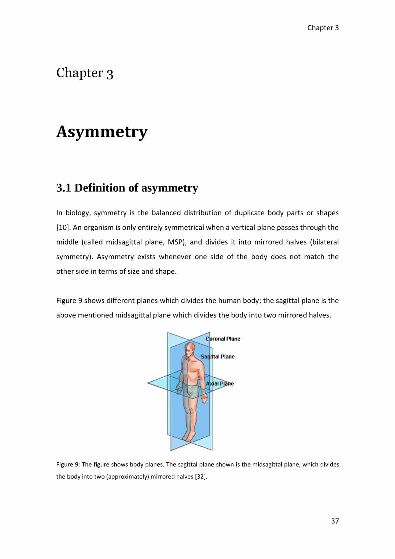
In biology, symmetry is the balanced distribution of duplicate body parts or shapes
[10]. An organism is only entirely symmetrical when a vertical plane passes through the
middle (called midsagittal plane, MSP), and divides it into mirrored halves (bilateral
symmetry). Asymmetry exists whenever one side of the body does not match the
other side in terms of size and shape.
Figure 9 shows different planes which divides the human body; the sagittal plane is the
above mentioned midsagittal plane which divides the body into two mirrored halves.
Figure 9: The figure shows body planes. The sagittal plane shown is the midsagittal plane, which divides
the body into two (approximately) mirrored halves [32].
Chapter 3
38
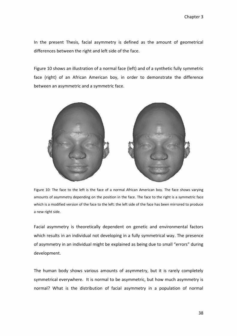
In the present Thesis, facial asymmetry is defined as the amount of geometrical
differences between the right and left side of the face.
Figure 10 shows an illustration of a normal face (left) and of a synthetic fully symmetric
face (right) of an African American boy, in order to demonstrate the difference
between an asymmetric and a symmetric face.
Figure 10: The face to the left is the face of a normal African American boy. The face shows varying
amounts of asymmetry depending on the position in the face. The face to the right is a symmetric face
which is a modified version of the face to the left: the left side of the face has been mirrored to produce
a new right side.
Facial asymmetry is theoretically dependent on genetic and environmental factors
which results in an individual not developing in a fully symmetrical way. The presence
of asymmetry in an individual might be explained as being due to small “errors” during
development.
The human body shows various amounts of asymmetry, but it is rarely completely
symmetrical everywhere. It is normal to be asymmetric, but how much asymmetry is
normal? What is the distribution of facial asymmetry in a population of normal
Chapter 3
39
children? Answering these questions is one of the main goals of the present Thesis. It is
sought answered by analyzing a number of facial surface scans of normal children.
Here, normality is defined in terms of the child not having had any known history of
congenital or acquired craniofacial deformity.
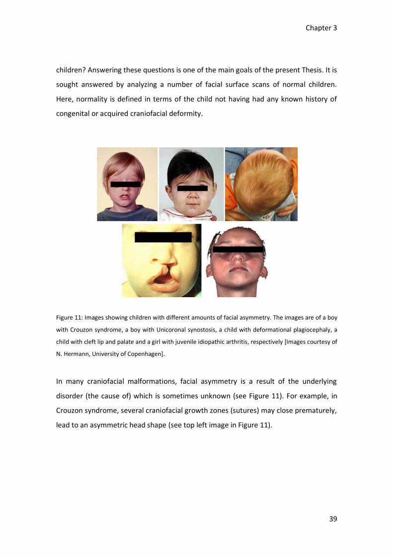
Figure 11: Images showing children with different amounts of facial asymmetry. The images are of a boy
with Crouzon syndrome, a boy with Unicoronal synostosis, a child with deformational plagiocephaly, a
child with cleft lip and palate and a girl with juvenile idiopathic arthritis, respectively [Images courtesy of
N. Hermann, University of Copenhagen].
In many craniofacial malformations, facial asymmetry is a result of the underlying
disorder (the cause of) which is sometimes unknown (see Figure 11). For example, in
Crouzon syndrome, several craniofacial growth zones (sutures) may close prematurely,
lead to an asymmetric head shape (see top left image in Figure 11).
Chapter 3
40
3.2 Fluctuating Asymmetry
Fluctuating asymmetry (FA) is the variability of left-right differences among individuals.
It is believed to be a measure of an individual’s genetic quality which is caused from
inability of the organism to develop in correctly determined paths [21]. Variations
between bilaterally symmetrical traits are seen as FA reflecting small accidents during
development. Random events in the outside environment have been found to be more
or less efficient in increasing FA which means that FA is increased by stress factors of
various kinds [18].
3.3 Directional Asymmetry
Directional asymmetry is the average difference between the two sides of the face
[14]. It occurs when there is a greater development on one side of the body [21].
Chapter 4
41
Chapter 4
Shape Analysis
4.1 Shape
The word “shape” is normally refering to the form of an object. In our case, the shape
is the surface of the face. The definition of shape is intuitively defined by D.G. Kendall
(1977):
“Shape is all the geometrical information that remains when location, scale and
rotational effects are filtered out from an object.” *7]
This means that when two objects have the same shape; they will exactly fit each other
if one of the objects is translated, rotated and scaled appropriately to best match the
other object.
4.2 Template
In image analysis, a template is often a representation of an “average” or “typical”
object. A template may also be used for studying the asymmetry in a face and in this
case, a symmetrical template is used. A symmetrical template is fully symmetric across
the MSP (midsagittal plane) and therefore contains implicit knowledge of one-to-one
correspondence of point locations between the right and left halves of the face.

Chapter 4
42
4.3 Landmarks
Shapes are often represented by a number of points which are called landmarks:
“A landmark is a point of correspondence on each object that matches between and
within populations.” *7]
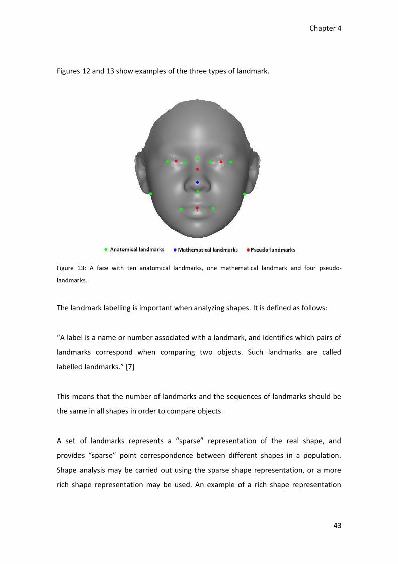
There exist three main types of landmarks: Anatomical, mathematical and pseudo-
landmarks [7]:
An anatomical landmark is a point (typically placed by an expert) that
corresponds between objects in a biological meaningful way, e.g. the inner
corner of an eye or the nasion.
Mathematical landmarks are points located on an object according to some
mathematical or geometrical feature, e.g. at an extreme point.
Pseudo-landmarks are constructed points on an object. The location of the
point depends on other landmarks, e.g. a point located between anatomical or
mathematical landmarks.
Figure 12: A vertebra of a mouse with six mathematical landmarks and 20 pseudo-landmarks. The figure
is modified from [7] page 4.
Chapter 4
43
Figures 12 and 13 show examples of the three types of landmark.
Figure 13: A face with ten anatomical landmarks, one mathematical landmark and four pseudo-
landmarks.
The landmark labelling is important when analyzing shapes. It is defined as follows:
“A label is a name or number associated with a landmark, and identifies which pairs of
landmarks correspond when comparing two objects. Such landmarks are called
labelled landmarks.” *7]
This means that the number of landmarks and the sequences of landmarks should be
the same in all shapes in order to compare objects.
A set of landmarks represents a “sparse” representation of the real shape, and
provides “sparse” point correspondence between different shapes in a population.
Shape analysis may be carried out using the sparse shape representation, or a more
rich shape representation may be used. An example of a rich shape representation

Chapter 4
44
would be the spatially dense set of points provided by a surface scanner. However, a
surface scan provides no implicit knowledge of point correspondences between scans
of different subjects. Therefore, before shape analysis can take place using the rich
point representation, so-called detailed point correspondence must be established.
4.4 Establishment of detailed point correspondence
Surface registration is needed in order to establish detailed point correspondence
between two surfaces. Surface registration is the process of transforming one surface
to align with another surface so that corresponding features or shapes can easily be
compared.
In the present project, two types of non-rigid registration are used:
A “Manual” (Landmark based method), where landmarks (control points) are
manually placed. Control points are used in rigid and non-rigid registration of
one surface relative to another surface.
An “Automatic” (Surface based method), where one surface is automatically
rigidly and non-rigidly registered to another surface based on surface
properties.
4.5 Surface transformation
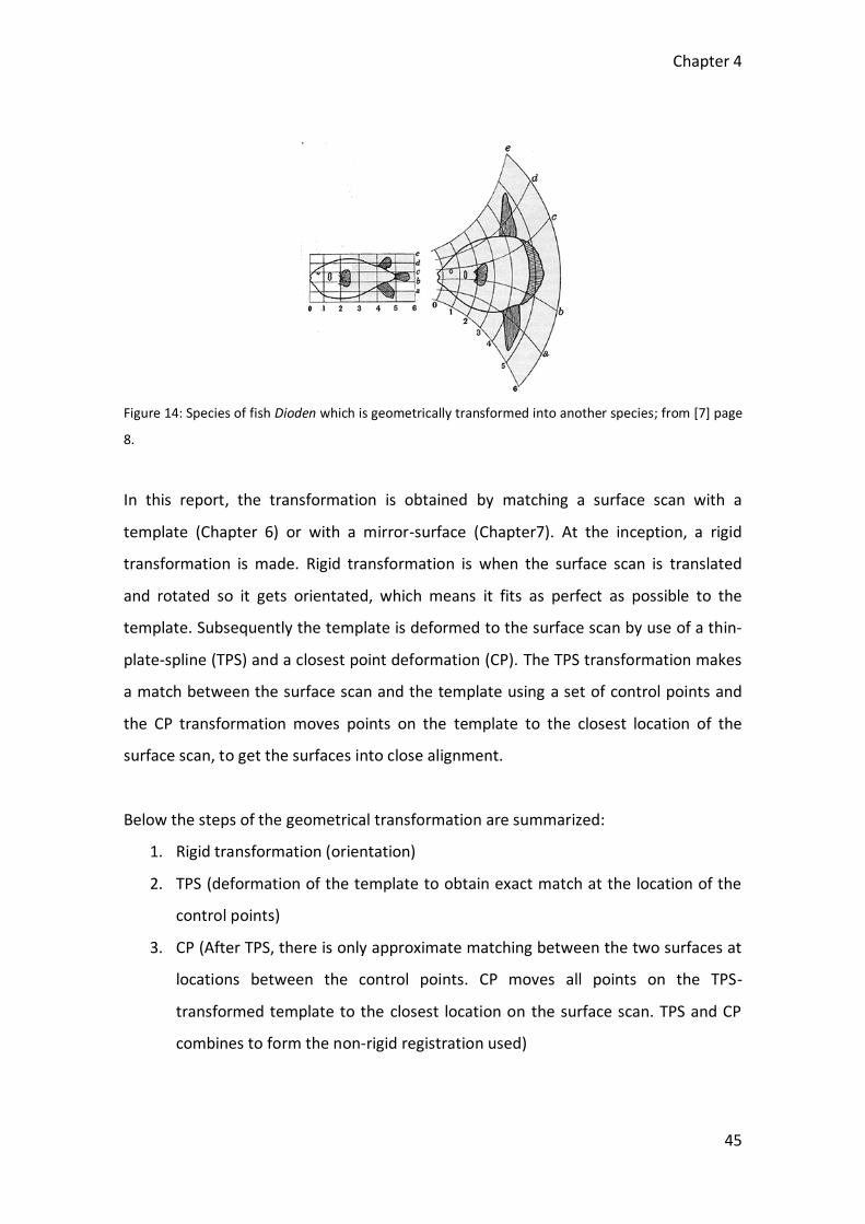
The purpose of registration is to transform the source shape into the coordinate
system of the target shape [7] (Figure 14). Figure 14 illustrates D´arcy Thompson´s
(1917) well-known example of a species of fish Dioden which is geometrically
transformed into another species. As it can be seen from the figure, a non-rigid
transformation is needed.
Chapter 4
45
Figure 14: Species of fish Dioden which is geometrically transformed into another species; from [7] page
8.
In this report, the transformation is obtained by matching a surface scan with a
template (Chapter 6) or with a mirror-surface (Chapter7). At the inception, a rigid
transformation is made. Rigid transformation is when the surface scan is translated
and rotated so it gets orientated, which means it fits as perfect as possible to the
template. Subsequently the template is deformed to the surface scan by use of a thin-
plate-spline (TPS) and a closest point deformation (CP). The TPS transformation makes
a match between the surface scan and the template using a set of control points and
the CP transformation moves points on the template to the closest location of the
surface scan, to get the surfaces into close alignment.
Below the steps of the geometrical transformation are summarized:
1. Rigid transformation (orientation)
2. TPS (deformation of the template to obtain exact match at the location of the
control points)
3. CP (After TPS, there is only approximate matching between the two surfaces at
locations between the control points. CP moves all points on the TPS-
transformed template to the closest location on the surface scan. TPS and CP
combines to form the non-rigid registration used)
Chapter 4
46
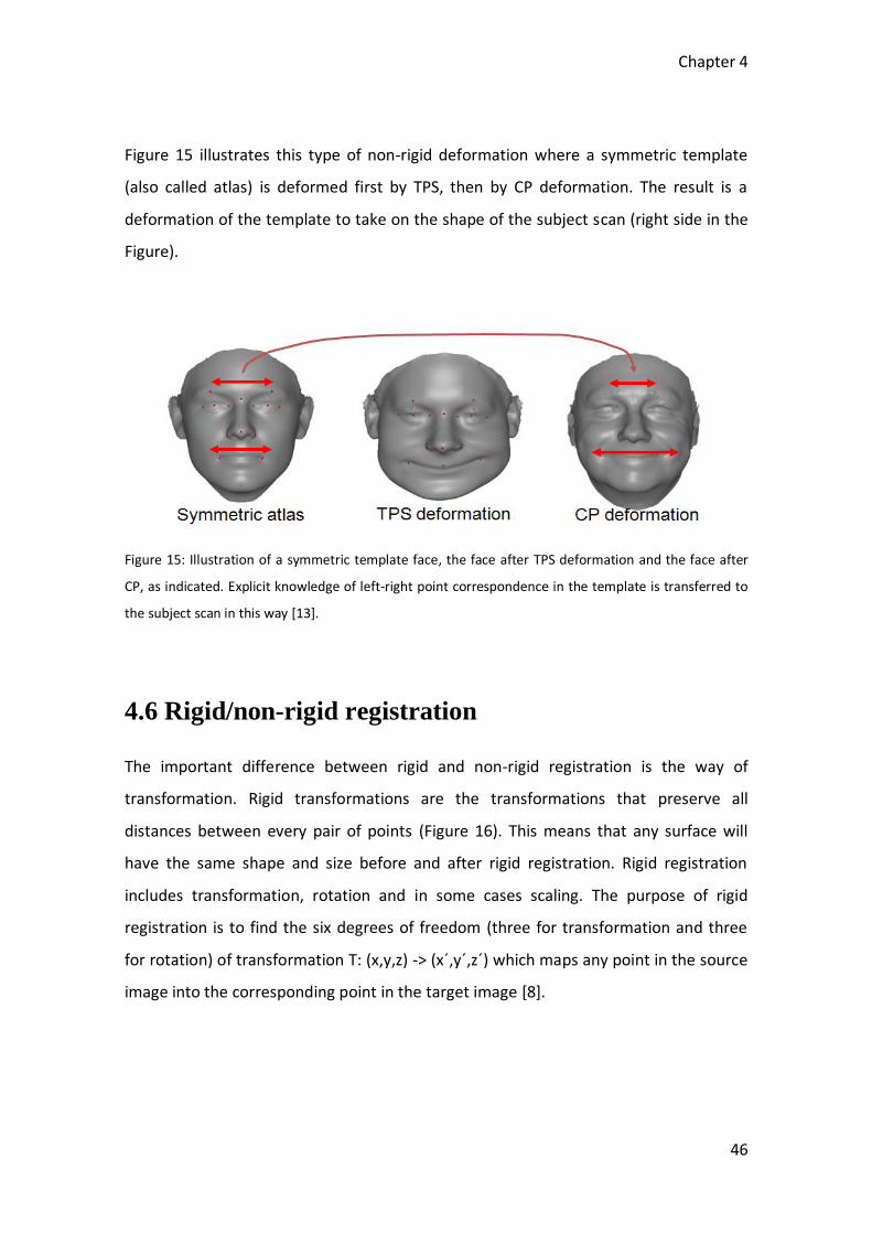
Figure 15 illustrates this type of non-rigid deformation where a symmetric template
(also called atlas) is deformed first by TPS, then by CP deformation. The result is a
deformation of the template to take on the shape of the subject scan (right side in the
Figure).
Figure 15: Illustration of a symmetric template face, the face after TPS deformation and the face after
CP, as indicated. Explicit knowledge of left-right point correspondence in the template is transferred to
the subject scan in this way [13].
4.6 Rigid/non-rigid registration
The important difference between rigid and non-rigid registration is the way of
transformation. Rigid transformations are the transformations that preserve all
distances between every pair of points (Figure 16). This means that any surface will
have the same shape and size before and after rigid registration. Rigid registration
includes transformation, rotation and in some cases scaling. The purpose of rigid
registration is to find the six degrees of freedom (three for transformation and three
for rotation) of transformation T: (x,y,z) -> (x´,y´,z´) which maps any point in the source
image into the corresponding point in the target image [8].

Chapter 4
47
Figure 16: An illustration of the difference between rigid/non-rigid registrations.
4.7 Thin-Plate Splines
Thin-plate splines (TPS) are a non-rigid transformation which is introduced for
statistical shape analysis. TPS are a part of the family of splines that are based on radial
basis functions. Radial basis function splines can be defined as a linear combination of
n radial basis functions θ(s).
Here, the transformation is defined as three separate TPS functions T = (t1, t2, t3)T. The
function yields a mapping between images, where the coefficients a describes the
affine part and b describes the non-affine part of the spline-based transformation and
describe the location of the control points [6].
Chapter 4
48
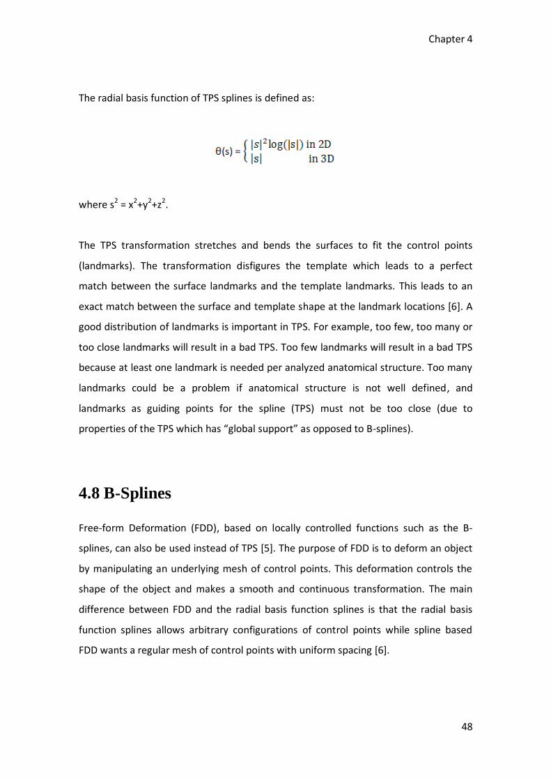
The radial basis function of TPS splines is defined as:
where s2 = x2+y2+z2.
The TPS transformation stretches and bends the surfaces to fit the control points
(landmarks). The transformation disfigures the template which leads to a perfect
match between the surface landmarks and the template landmarks. This leads to an
exact match between the surface and template shape at the landmark locations [6]. A
good distribution of landmarks is important in TPS. For example, too few, too many or
too close landmarks will result in a bad TPS. Too few landmarks will result in a bad TPS
because at least one landmark is needed per analyzed anatomical structure. Too many
landmarks could be a problem if anatomical structure is not well defined, and
landmarks as guiding points for the spline (TPS) must not be too close (due to
properties of the TPS which has “global support” as opposed to B-splines).
4.8 B-Splines
Free-form Deformation (FDD), based on locally controlled functions such as the B-
splines, can also be used instead of TPS [5]. The purpose of FDD is to deform an object
by manipulating an underlying mesh of control points. This deformation controls the
shape of the object and makes a smooth and continuous transformation. The main
difference between FDD and the radial basis function splines is that the radial basis
function splines allows arbitrary configurations of control points while spline based
FDD wants a regular mesh of control points with uniform spacing [6].
Chapter 4
49
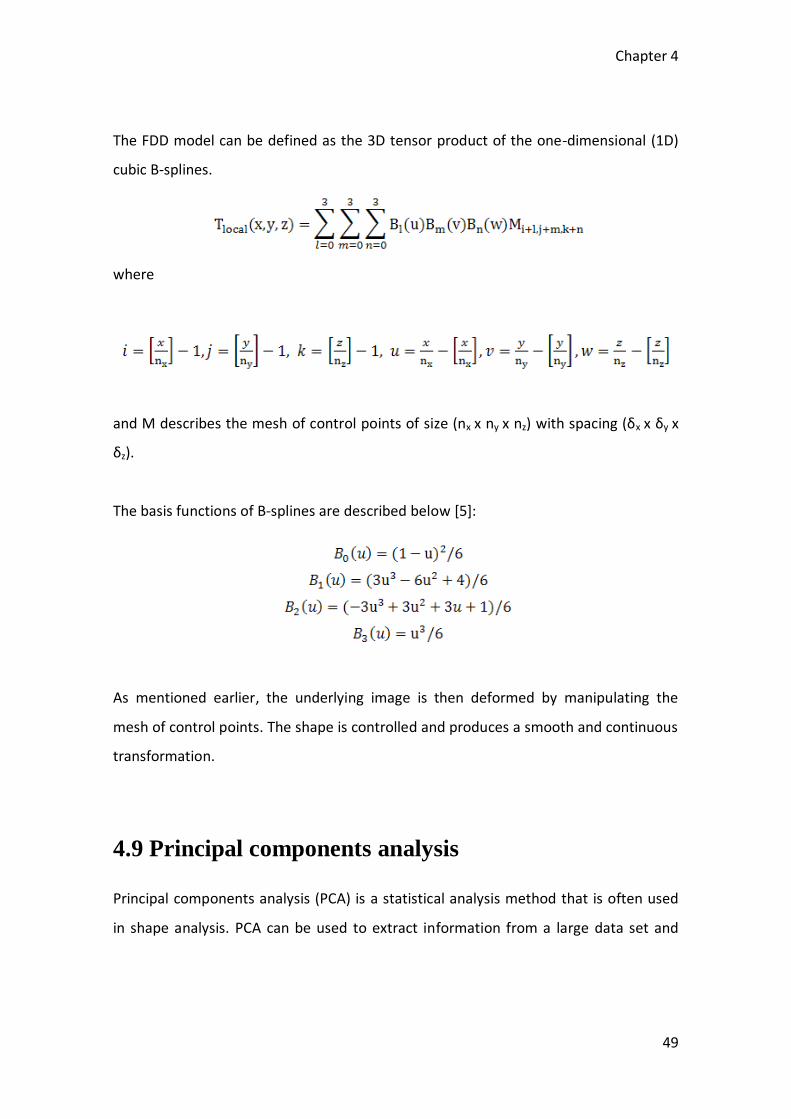
The FDD model can be defined as the 3D tensor product of the one-dimensional (1D)
cubic B-splines.
where
and M describes the mesh of control points of size (nx x ny x nz) with spacing (δx x δy x
δz).
The basis functions of B-splines are described below [5]:
As mentioned earlier, the underlying image is then deformed by manipulating the
mesh of control points. The shape is controlled and produces a smooth and continuous
transformation.
4.9 Principal components analysis
Principal components analysis (PCA) is a statistical analysis method that is often used
in shape analysis. PCA can be used to extract information from a large data set and
Chapter 4
50
provides information about the dominant (and often important) types of variation in
the data [7].
PCA is also a variable reduction procedure. The analysis can be used if there is some
redundancy in the variables. This means that some of the variables are correlated with
one another. Consequently it is possible to reduce the observed variables into a
smaller number of principal components (artificial variables) which will give an
explanation of the variance in the observed variables. PCA will find the eigenvectors
corresponding to the largest eigenvalues of the covariance matrix; which means PCA
will find the directions in the data with the most variation [31].
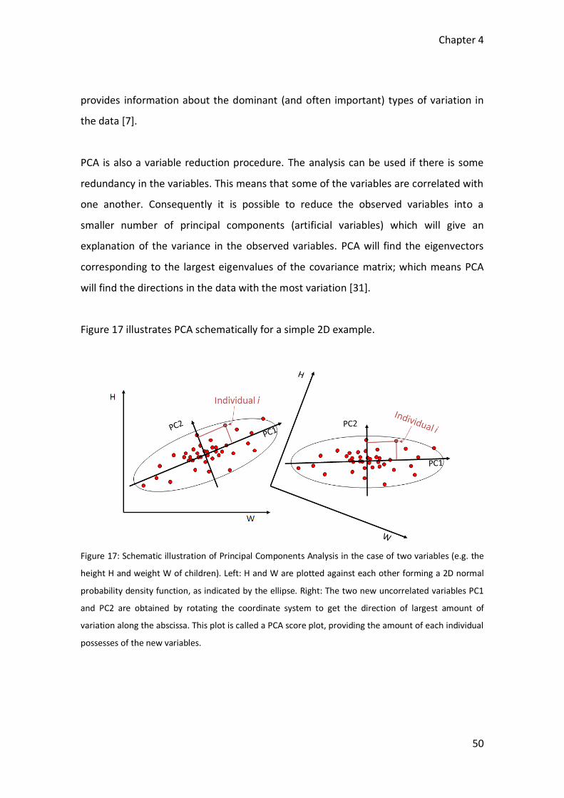
Figure 17 illustrates PCA schematically for a simple 2D example.
Figure 17: Schematic illustration of Principal Components Analysis in the case of two variables (e.g. the
height H and weight W of children). Left: H and W are plotted against each other forming a 2D normal
probability density function, as indicated by the ellipse. Right: The two new uncorrelated variables PC1
and PC2 are obtained by rotating the coordinate system to get the direction of largest amount of
variation along the abscissa. This plot is called a PCA score plot, providing the amount of each individual
possesses of the new variables.
Chapter 5
51
Chapter 5
Quantification of facial asymmetry
at manually placed landmark
locations
5.1 Introduction
In this chapter, a method is developed for quantification of facial asymmetry. The
method is tested on a small group of children of different ages, gender and ethnicity.
An asymmetry measure is defined and used in order to estimate the facial asymmetry
in a sparse set of manually placed landmark locations. A deviation from the mean
asymmetry is then estimated for each face and in different landmark locations for
every face. Afterwards, a relation is investigated between asymmetry and the age of
children and the difference between boys and girls is also studied. Another purpose of
this chapter is to study how the manual landmarking impacts on the measured amount
of asymmetry. This is implemented by landmarking the same faces twice with a 2-3
weeks interval, thus providing a measure of reproducibility. The results are validated
and discussed at the end.
The developed methodology will be applied to a larger population in Chapter 8.

Chapter 5
52
5.2 Material
In this chapter, manually placed landmarks for 30 3D facial surface scans are used. The
landmarks are anatomically localized on the face surfaces. Eight of the 30 surface scans
derived from African American boys, eight of them derived from Caucasian boys, seven
of the surface scans derived from African American girls and seven of them derived
from Caucasian girls. Figure 18 shows an illustration of the 18 landmarks used.
Figure 18: The surface to the left is a surface representation of the face of a normal Caucasian boy.
Landmarks (red spheres) are placed on the surface in various anatomical locations. For clarity, the figure
to the right shows the landmarks without showing the corresponding facial surface.
5.3 Method
The asymmetry measure requires establishment of a sparse set of manually placed
landmarks representing left-right correspondences in the face. Before the calculation
of the asymmetry, the landmarks are oriented to the landmark of a standard oriented
symmetric template of landmarks using rigid transformation based on all landmarks.
Chapter 5
53
The result is translated in such a manner that the midpoint between ear landmarks for
the 30 surface scans and for the template coincide.
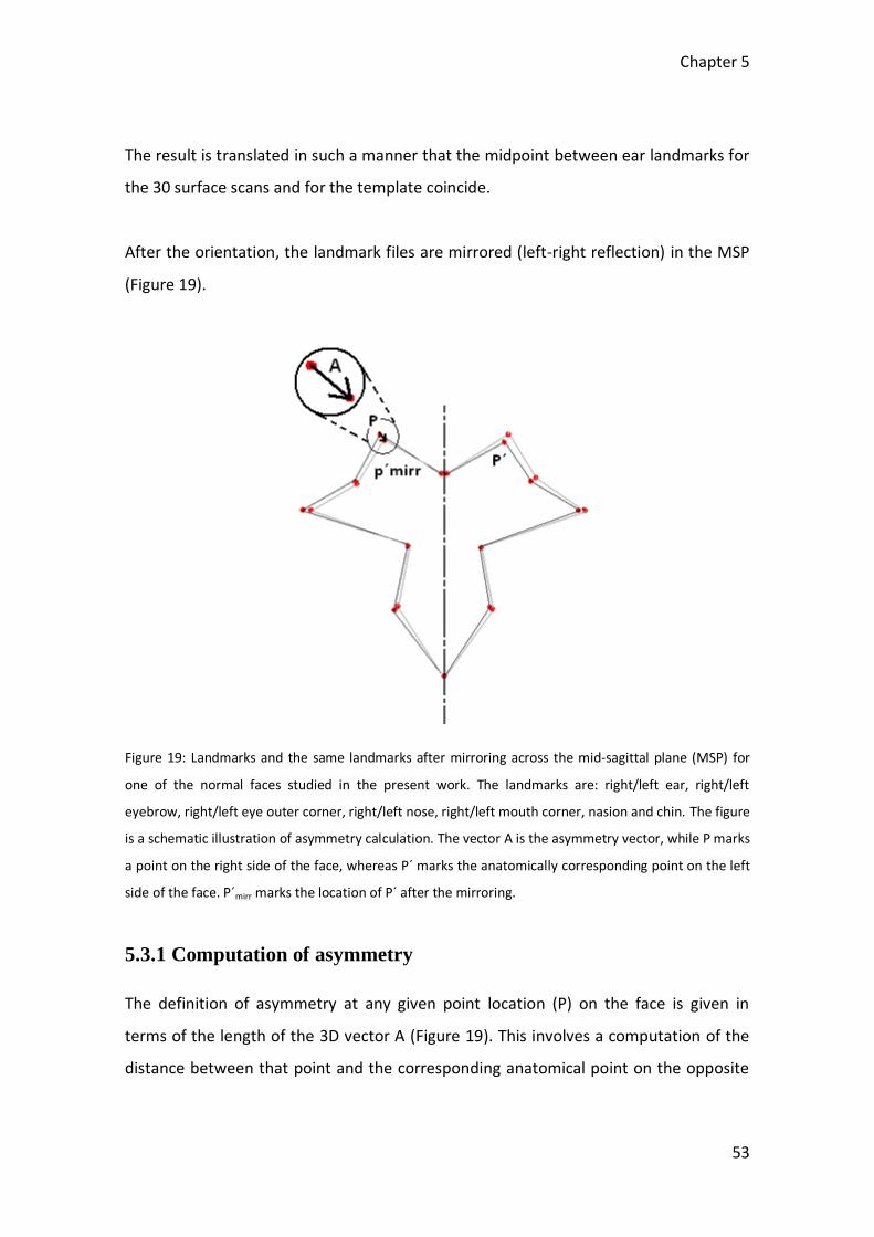
After the orientation, the landmark files are mirrored (left-right reflection) in the MSP
(Figure 19).
Figure 19: Landmarks and the same landmarks after mirroring across the mid-sagittal plane (MSP) for
one of the normal faces studied in the present work. The landmarks are: right/left ear, right/left
eyebrow, right/left eye outer corner, right/left nose, right/left mouth corner, nasion and chin. The figure
is a schematic illustration of asymmetry calculation. The vector A is the asymmetry vector, while P marks
a point on the right side of the face, whereas P´ marks the anatomically corresponding point on the left
side of the face. P´mirr marks the location of P´ after the mirroring.
5.3.1 Computation of asymmetry
The definition of asymmetry at any given point location (P) on the face is given in
terms of the length of the 3D vector A (Figure 19). This involves a computation of the
distance between that point and the corresponding anatomical point on the opposite

Chapter 5
54
side of the MSP after mirroring across the MSP (P´mirr). The length of A provides the
magnitude of asymmetry while the Cartesian components of A provide the amount of
asymmetry in the transverse, vertical and sagittal directions, respectively, in the face.
The vector B (containing all 18 landmark locations for all subjects) consists of an mx3xn
matrix, where m is the number of landmarks, 3 for the Cartesian vector component
(x,y,z) and n is the number of faces. The first eight (number 1-8) landmarks of the
matrix are located on the right side of the face and the last eight landmarks (number
13-18) are the corresponding landmarks on the left side of the face. Landmark
numbers 9-12 are located in the middle of the face (nasion, nose tip etc.).
Figure 20 shows all landmark coordinates (x, y and z) for all 30 faces. As seen, the same
landmark for different faces is located almost in the same location. This is also made
clear in Figure 21 (plot to the right) where the x and y landmarks of all faces are
plotted.
Figure 20: The figure shows the x; y; and z position of all landmarks for all 30 faces.
0 2 4 6 8 10 12 14 16 18-100
0
100
Landmark number
x-v
alu
es
x, y and z values for landmarks
0 2 4 6 8 10 12 14 16 18-100
0
100
Landmark number
y-v
alu
es
0 2 4 6 8 10 12 14 16 18-200
0
200
Landmark number
z-v
alu
es

Chapter 5
55
Figure 21: The figure to the left shows the x and y landmarks position of one face and the figure to the
right shows the x and y landmark values of all faces.
As described above, B contains both values from right and left side of the face.
Therefore, the vector (containing landmark locations for all subjects) for both right and
left side of the face is identical. This means that P is equal to P´. Subsequently P´mirr is
achieved by multiplying the x values of this vector by -1.
Re-development is then made for the P´mirr vector, where the first eight values are
interchanged with the last eight values of the vector. That is landmark numbers 1 and
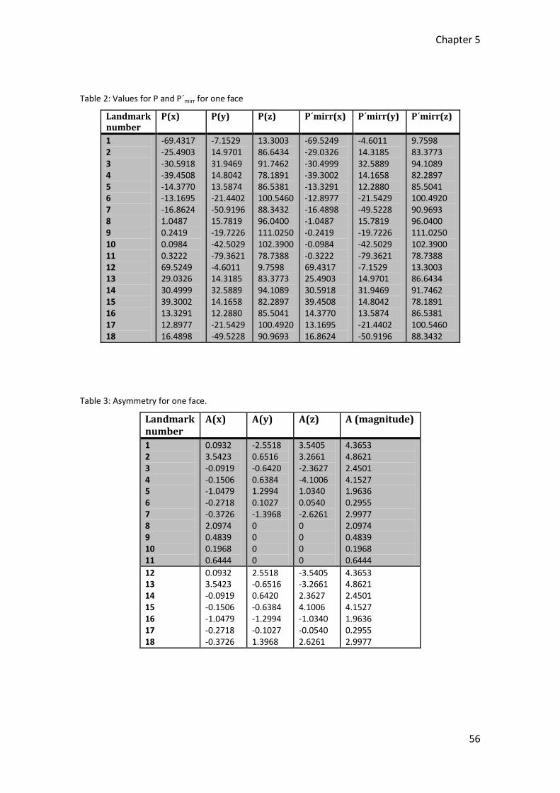
13, 2 and 14, 3 and 15 etc. are swapping their places (Table 2).
The asymmetry A is achieved by subtracting P from P´mirr (Table 3). It is seen from the
values of P and P´mirr the vector A can be truncated because after subtracting the two
vectors, the first eight values will be as the last eight values. This results that A
becomes a vector of size 11x3x30, where 11 is the number of point locations of P-P´mirr.
Figure 22 shows the asymmetry of x, y and z for every 30 faces for 11 landmarks used.
-80 -60 -40 -20 0 20 40 60 80-100
-80
-60
-40
-20
0
20
40
x-values
y-v
alu
es
Landmark position for x and y values of one face
-80 -60 -40 -20 0 20 40 60 80-100
-50
0
50
x-values
y-v
alu
es
Landmark position for x and y values of every face
Chapter 5
56
Table 2: Values for P and P´mirr for one face
Landmark number
P(x) P(y) P(z) P´mirr(x) P´mirr(y) P´mirr(z)
1 2 3 4 5 6 7 8 9 10 11 12 13 14 15 16 17 18
-69.4317 -25.4903 -30.5918 -39.4508 -14.3770 -13.1695 -16.8624 1.0487 0.2419 0.0984 0.3222 69.5249 29.0326 30.4999 39.3002 13.3291 12.8977 16.4898
-7.1529 14.9701 31.9469 14.8042 13.5874 -21.4402 -50.9196 15.7819 -19.7226 -42.5029 -79.3621 -4.6011 14.3185 32.5889 14.1658 12.2880 -21.5429 -49.5228
13.3003 86.6434 91.7462 78.1891 86.5381 100.5460 88.3432 96.0400 111.0250 102.3900 78.7388 9.7598 83.3773 94.1089 82.2897 85.5041 100.4920 90.9693
-69.5249 -29.0326 -30.4999 -39.3002 -13.3291 -12.8977 -16.4898 -1.0487 -0.2419 -0.0984 -0.3222 69.4317 25.4903 30.5918 39.4508 14.3770 13.1695 16.8624
-4.6011 14.3185 32.5889 14.1658 12.2880 -21.5429 -49.5228 15.7819 -19.7226 -42.5029 -79.3621 -7.1529 14.9701 31.9469 14.8042 13.5874 -21.4402 -50.9196
9.7598 83.3773 94.1089 82.2897 85.5041 100.4920 90.9693 96.0400 111.0250 102.3900 78.7388 13.3003 86.6434 91.7462 78.1891 86.5381 100.5460 88.3432
Table 3: Asymmetry for one face.
Landmark number
A(x) A(y) A(z) A (magnitude)
1 2 3 4 5 6 7 8 9 10 11
0.0932 3.5423 -0.0919 -0.1506 -1.0479 -0.2718 -0.3726 2.0974 0.4839 0.1968 0.6444
-2.5518 0.6516 -0.6420 0.6384 1.2994 0.1027 -1.3968 0 0 0 0
3.5405 3.2661 -2.3627 -4.1006 1.0340 0.0540 -2.6261 0 0 0 0
4.3653 4.8621 2.4501 4.1527 1.9636 0.2955 2.9977 2.0974 0.4839 0.1968 0.6444
12 13 14 15 16 17 18
0.0932 3.5423 -0.0919 -0.1506 -1.0479 -0.2718 -0.3726
2.5518 -0.6516 0.6420 -0.6384 -1.2994 -0.1027 1.3968
-3.5405 -3.2661 2.3627 4.1006 -1.0340 -0.0540 2.6261
4.3653 4.8621 2.4501 4.1527 1.9636 0.2955 2.9977

Chapter 5
57
Figure 22: Asymmetry values in x, y and z directions, respectively, for all 30 faces.
The asymmetry
is found for every face and for every landmark point in every face. Subsequently the
mean, standard deviation, maximum and minimum values are found for the
asymmetry.
where n is number of subjects. Subsequently, a deviation is computed by subtracting
the asymmetry from the mean.
1 2 3 4 5 6 7 8 9 10 11-10
0
10
Landmark numberx-v
alu
es
x, y and z values of asymmetry of landmarks
1 2 3 4 5 6 7 8 9 10 11-10
0
10
Landmark number
y-v
alu
es
1 2 3 4 5 6 7 8 9 10 11-10
0
10
Landmark number
z-v
alu
es
Chapter 5
58
5.3.2 Implementation
The asymmetry quantification was implemented in Matlab (Matrix Laboratory). Firstly,
the log files for the landmarks are read in Matlab. Then the asymmetry and the
deviation are estimated. Subsequently, the asymmetry is plotted against the age of the
children and then a comparison is made between girls and boys (see Appendix C.1 for
Matlab script).
5.3.3 Error due to manual landmarking
The manual landmarking process contributes an error to the quantification of
asymmetry. In order to estimate the magnitude of landmarking error, the faces were
landmarked twice within a 2-3 weeks interval. This was done using the software
program Landmarker [Darvann 2008]. An error signal E was estimated, where E
represents the distance between coordinates of a landmark from the first and second
landmarking, respectively. This definition makes E an effective “asymmetry”-like signal
that may be directly compared to the magnitude of the A-vector which has a
contribution from both asymmetry and landmarking error. A root-mean-square error
(RMS) is calculated for both A and E, respectively, for each landmark.
5.4 Results
In this section, the results of the asymmetry quantification are presented. The results
consist of the asymmetry for all of the n=30 faces at each landmark location. The
asymmetry estimation is presented twice since the faces are landmarked twice to
determine how the manual landmarking impacts the measured amount of asymmetry.
A deviation from the mean asymmetry is also estimated for the amount of asymmetry
in each face and for each landmark location. Subsequently, results of the study of the
Chapter 5
59
difference between boys and girls and the result of the relation between asymmetry
and age are presented.
5.4.1 Asymmetry computation
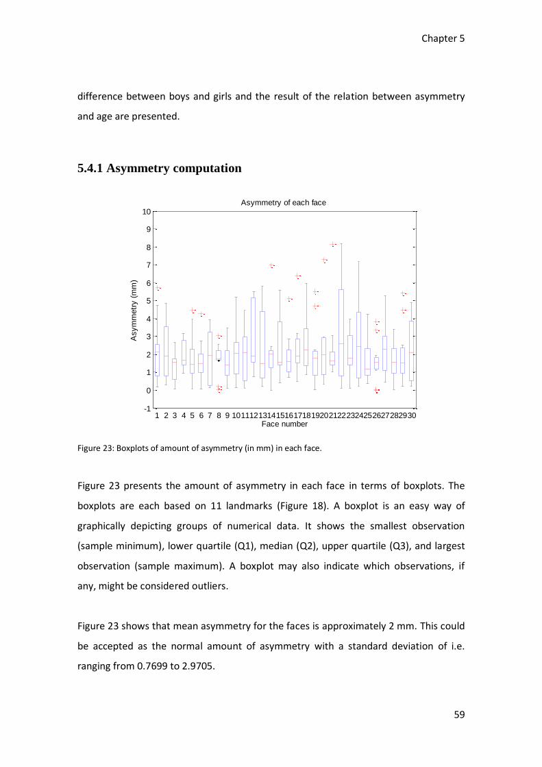
Figure 23: Boxplots of amount of asymmetry (in mm) in each face.
Figure 23 presents the amount of asymmetry in each face in terms of boxplots. The
boxplots are each based on 11 landmarks (Figure 18). A boxplot is an easy way of
graphically depicting groups of numerical data. It shows the smallest observation
(sample minimum), lower quartile (Q1), median (Q2), upper quartile (Q3), and largest
observation (sample maximum). A boxplot may also indicate which observations, if
any, might be considered outliers.
Figure 23 shows that mean asymmetry for the faces is approximately 2 mm. This could
be accepted as the normal amount of asymmetry with a standard deviation of i.e.
ranging from 0.7699 to 2.9705.
-1
0
1
2
3
4
5
6
7
8
9
10
1 2 3 4 5 6 7 8 9 101112131415161718192021222324252627282930Face number
Asym
metr
y (
mm
)
Asymmetry of each face

Chapter 5
60
Table 4: Mean asymmetry and standard deviation for landmarks.
Figure 24: Asymmetry values (in mm) for each landmark point in all faces (see figure 18 for location of
landmarks).
The asymmetry values for each landmark point for each face are seen in Figure 24. The
table next to the figure provides the mean asymmetry values and standard deviation
values for each landmark.
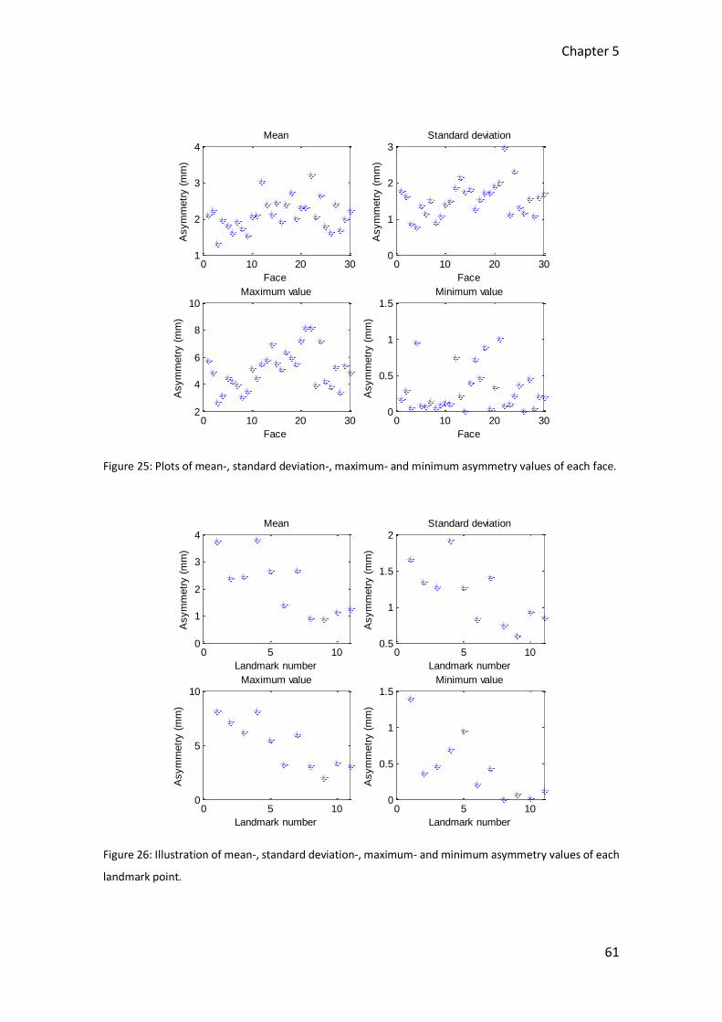
Figure 25 shows the asymmetry values for the mean, standard deviation, maximum
and minimum of each face.
Figure 26 is similar to figure 25. Here the mean, standard deviation, maximum and
minimum asymmetry values of each landmark point are plotted.
Landmark number
Mean asymmetry
Mean Standard deviation
1 2 3 4 5 6 7 8 9 10 11
3.7513 2.3842 2.4602 3.8046 2.6391 1.3967 2.6794 0.9244 0.8971 1.1482 1.2678
1.6608 1.3397 1.2725 1.9138 1.2674 0.8336 1.4075 0.7430 0.5984 0.9329 0.8493
1 2 3 4 5 6 7 8 9 10 110
1
2
3
4
5
6
7
8
9
Landmark
Asym
metr
y
Asymmetri values of each point in all faces
Chapter 5
61
Figure 25: Plots of mean-, standard deviation-, maximum- and minimum asymmetry values of each face.
Figure 26: Illustration of mean-, standard deviation-, maximum- and minimum asymmetry values of each
landmark point.
0 10 20 301
2
3
4
Face
Asym
metr
y (
mm
)
Mean
0 10 20 300
1
2
3
Face
Asym
metr
y (
mm
)
Standard deviation
0 10 20 302
4
6
8
10
Face
Asym
metr
y (
mm
)
Maximum value
0 10 20 300
0.5
1
1.5
Face
Asym
metr
y (
mm
)
Minimum value
0 5 100
1
2
3
4
Landmark number
Asym
metr
y (
mm
)
Mean
0 5 100.5
1
1.5
2
Landmark number
Asym
metr
y (
mm
)
Standard deviation
0 5 100
5
10
Landmark number
Asym
metr
y (
mm
)
Maximum value
0 5 100
0.5
1
1.5
Landmark number
Asym
metr
y (
mm
)
Minimum value
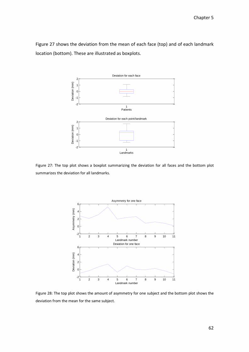
Chapter 5
62
Figure 27 shows the deviation from the mean of each face (top) and of each landmark
location (bottom). These are illustrated as boxplots.
Figure 27: The top plot shows a boxplot summarizing the deviation for all faces and the bottom plot
summarizes the deviation for all landmarks.
Figure 28: The top plot shows the amount of asymmetry for one subject and the bottom plot shows the
deviation from the mean for the same subject.
-2
-1
0
1
2
1Patients
Devia
tion (
mm
)
Deviation for each face
-2
-1
0
1
2
1Landmarks
Devia
tion (
mm
)
Deviation for each point/landmark
1 2 3 4 5 6 7 8 9 10 11-2
0
2
4
6
Landmark number
Asym
metr
y (
mm
)
Asymmetry for one face
1 2 3 4 5 6 7 8 9 10 11-2
0
2
4
6
Landmark number
Devia
tion (
mm
)
Deviation for one face
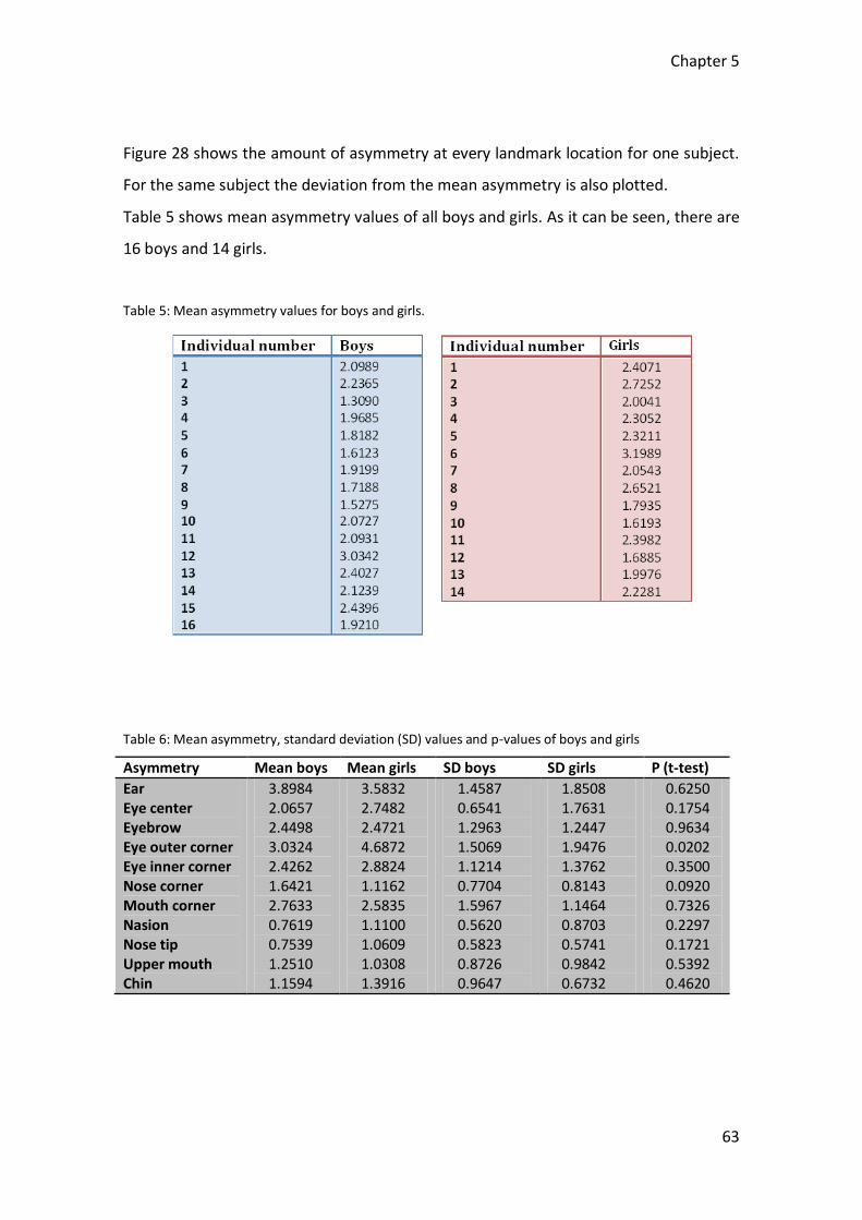
Chapter 5
63
Figure 28 shows the amount of asymmetry at every landmark location for one subject.
For the same subject the deviation from the mean asymmetry is also plotted.
Table 5 shows mean asymmetry values of all boys and girls. As it can be seen, there are
16 boys and 14 girls.
Table 5: Mean asymmetry values for boys and girls.
Table 6: Mean asymmetry, standard deviation (SD) values and p-values of boys and girls
Asymmetry Mean boys Mean girls SD boys SD girls P (t-test)
Ear Eye center Eyebrow Eye outer corner Eye inner corner Nose corner Mouth corner Nasion Nose tip Upper mouth Chin
3.8984 2.0657 2.4498 3.0324 2.4262 1.6421 2.7633 0.7619 0.7539 1.2510 1.1594
3.5832 2.7482 2.4721 4.6872 2.8824 1.1162 2.5835 1.1100 1.0609 1.0308 1.3916
1.4587 0.6541 1.2963 1.5069 1.1214 0.7704 1.5967 0.5620 0.5823 0.8726 0.9647
1.8508 1.7631 1.2447 1.9476 1.3762 0.8143 1.1464 0.8703 0.5741 0.9842 0.6732
0.6250 0.1754 0.9634 0.0202 0.3500 0.0920 0.7326 0.2297 0.1721 0.5392 0.4620
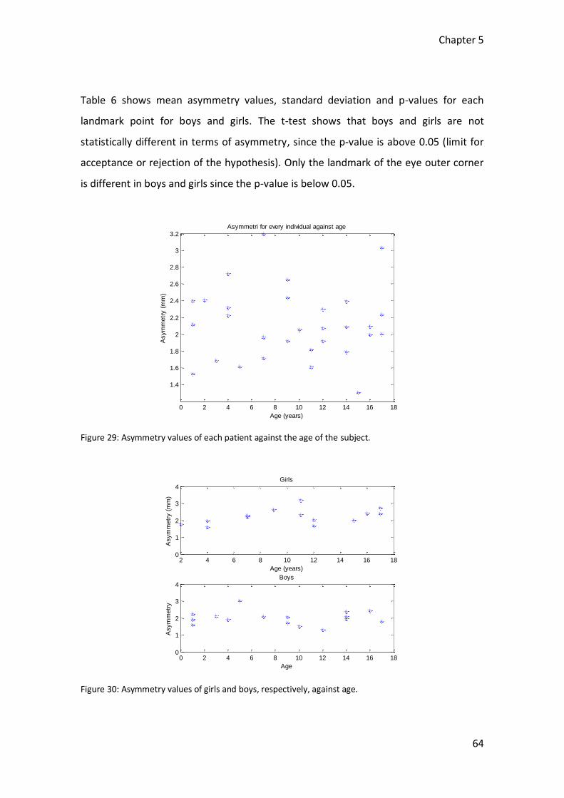
Chapter 5
64
Table 6 shows mean asymmetry values, standard deviation and p-values for each
landmark point for boys and girls. The t-test shows that boys and girls are not
statistically different in terms of asymmetry, since the p-value is above 0.05 (limit for
acceptance or rejection of the hypothesis). Only the landmark of the eye outer corner
is different in boys and girls since the p-value is below 0.05.
Figure 29: Asymmetry values of each patient against the age of the subject.
Figure 30: Asymmetry values of girls and boys, respectively, against age.
0 2 4 6 8 10 12 14 16 18
1.4
1.6
1.8
2
2.2
2.4
2.6
2.8
3
3.2
Age (years)
Asym
metr
y (
mm
)
Asymmetri for every individual against age
2 4 6 8 10 12 14 16 180
1
2
3
4
Age (years)
Asym
metr
y (
mm
)
Girls
0 2 4 6 8 10 12 14 16 180
1
2
3
4
Age
Asym
metr
y
Boys
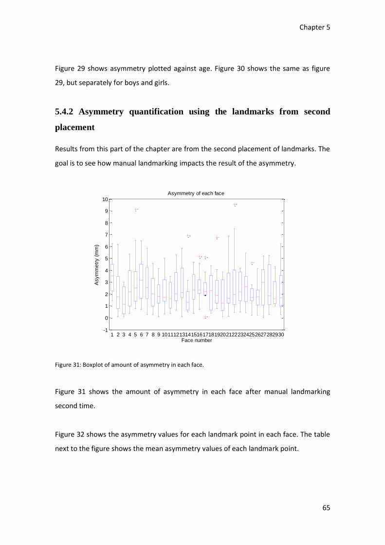
Chapter 5
65
Figure 29 shows asymmetry plotted against age. Figure 30 shows the same as figure
29, but separately for boys and girls.
5.4.2 Asymmetry quantification using the landmarks from second
placement
Results from this part of the chapter are from the second placement of landmarks. The
goal is to see how manual landmarking impacts the result of the asymmetry.
Figure 31: Boxplot of amount of asymmetry in each face.
Figure 31 shows the amount of asymmetry in each face after manual landmarking
second time.
Figure 32 shows the asymmetry values for each landmark point in each face. The table
next to the figure shows the mean asymmetry values of each landmark point.
-1
0
1
2
3
4
5
6
7
8
9
10
1 2 3 4 5 6 7 8 9 101112131415161718192021222324252627282930Face number
Asym
metr
y (
mm
)
Asymmetry of each face
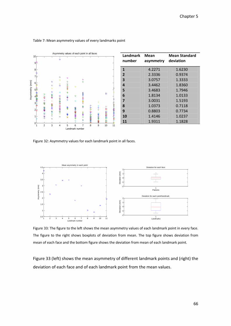
Chapter 5
66
Table 7: Mean asymmetry values of every landmarks point
Figure 32: Asymmetry values for each landmark point in all faces.
Figure 33: The figure to the left shows the mean asymmetry values of each landmark point in every face.
The figure to the right shows boxplots of deviation from mean. The top figure shows deviation from
mean of each face and the bottom figure shows the deviation from mean of each landmark point.
Figure 33 (left) shows the mean asymmetry of different landmark points and (right) the
deviation of each face and of each landmark point from the mean values.
1 2 3 4 5 6 7 8 9 10 110.5
1
1.5
2
2.5
3
3.5
4
4.5
Landmark number
Asym
metr
y (
mm
)
Mean asymmetry in each point
-2
-1
0
1
2
1Patients
Devia
tion (
mm
)
Deviation for each face
-2
-1
0
1
2
1Landmarks
Devia
tion (
mm
)
Deviation for each point/landmark
Landmark number
Mean asymmetry
Mean Standard deviation
1 2 3 4 5 6 7 8 9 10 11
4.2271 2.3336 3.0757 3.4462 3.4683 1.8134 3.0031 1.0373 0.8803 1.4146 1.9311
1.6230 0.9374 1.3333 1.8360 1.7946 1.0133 1.5193 0.7118 0.7734 1.0237 1.1828
1 2 3 4 5 6 7 8 9 10 110
1
2
3
4
5
6
7
8
9
10
Landmark number
Asym
metr
y (
mm
)
Asymmetry values of each point in all faces
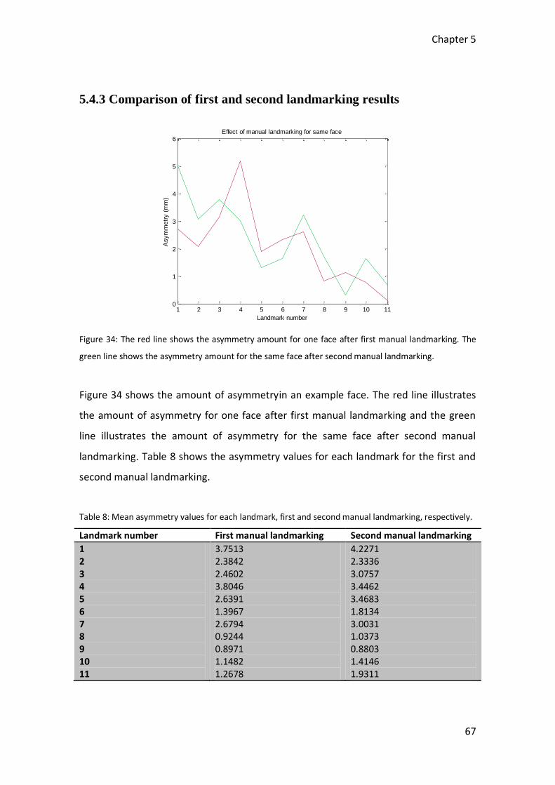
Chapter 5
67
5.4.3 Comparison of first and second landmarking results
Figure 34: The red line shows the asymmetry amount for one face after first manual landmarking. The
green line shows the asymmetry amount for the same face after second manual landmarking.
Figure 34 shows the amount of asymmetryin an example face. The red line illustrates
the amount of asymmetry for one face after first manual landmarking and the green
line illustrates the amount of asymmetry for the same face after second manual
landmarking. Table 8 shows the asymmetry values for each landmark for the first and
second manual landmarking.
Table 8: Mean asymmetry values for each landmark, first and second manual landmarking, respectively.
Landmark number First manual landmarking Second manual landmarking
1 2 3 4 5 6 7 8 9 10 11
3.7513 2.3842 2.4602 3.8046 2.6391 1.3967 2.6794 0.9244 0.8971 1.1482 1.2678
4.2271 2.3336 3.0757 3.4462 3.4683 1.8134 3.0031 1.0373 0.8803 1.4146 1.9311
1 2 3 4 5 6 7 8 9 10 110
1
2
3
4
5
6
Landmark number
Asym
metr
y (
mm
)
Effect of manual landmarking for same face
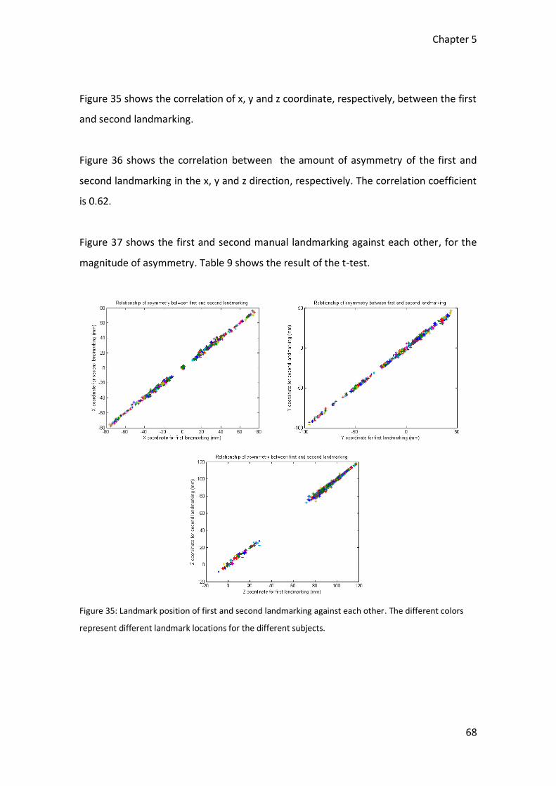
Chapter 5
68
Figure 35 shows the correlation of x, y and z coordinate, respectively, between the first
and second landmarking.
Figure 36 shows the correlation between the amount of asymmetry of the first and
second landmarking in the x, y and z direction, respectively. The correlation coefficient
is 0.62.
Figure 37 shows the first and second manual landmarking against each other, for the
magnitude of asymmetry. Table 9 shows the result of the t-test.
Figure 35: Landmark position of first and second landmarking against each other. The different colors
represent different landmark locations for the different subjects.
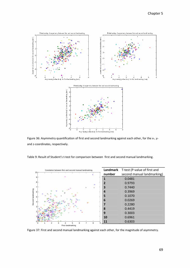
Chapter 5
69
Figure 36: Asymmetry quantification of first and second landmarking against each other, for the x-, y-
and z-coordinates, respectively.
Table 9: Result of Student’s t-test for comparison between first and second manual landmarking.
Figure 37: First and second manual landmarking against each other, for the magnitude of asymmetry.
0 1 2 3 4 5 6 7 8 90
1
2
3
4
5
6
7
8
9
10
First landmarking
Second landm
ark
ing
Correlation between first and second manual landmarking Landmark number
T-test (P-value of first and second manual landmarking)
1 2 3 4 5 6 7 8 9 10 11
0.0481 0.9793 0.7440 0.3969 0.1070 0.0269 0.2280 0.4419 0.3003 0.6961 0.6303
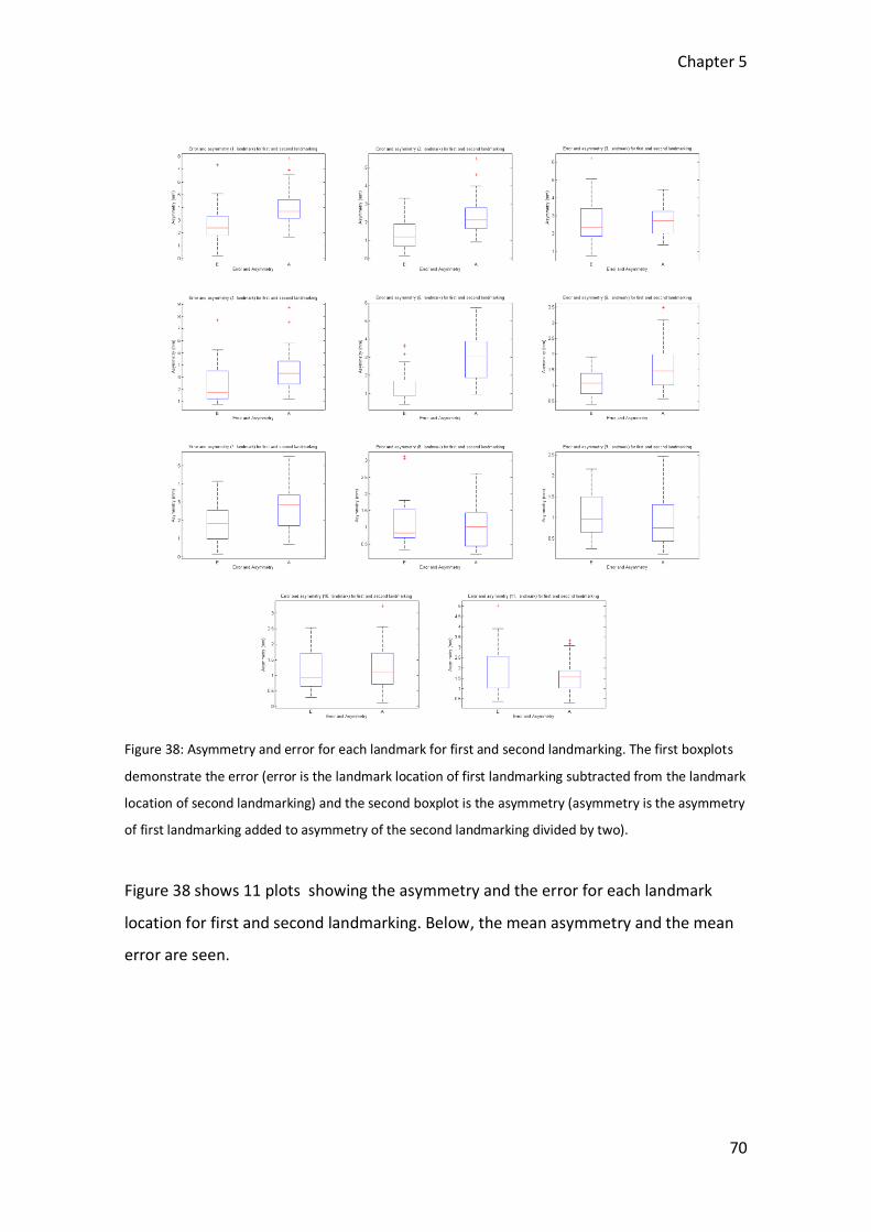
Chapter 5
70
Figure 38: Asymmetry and error for each landmark for first and second landmarking. The first boxplots
demonstrate the error (error is the landmark location of first landmarking subtracted from the landmark
location of second landmarking) and the second boxplot is the asymmetry (asymmetry is the asymmetry
of first landmarking added to asymmetry of the second landmarking divided by two).
Figure 38 shows 11 plots showing the asymmetry and the error for each landmark
location for first and second landmarking. Below, the mean asymmetry and the mean
error are seen.

Chapter 5
71
Figure 39: Mean asymmetry and mean error for all landmarks for first and second landmarking. The first
boxplot demonstrates the error (error is the mean of landmark location of first landmarking subtracted
from the mean of landmark location of second landmarking) and the second boxplot is the asymmetry
(asymmetry is the mean asymmetry of first landmarking added to mean asymmetry of the second
landmarking divided by two).
Table 10 shows the result of S/N ratio for the mean asymmetry. Also, RMS for the
error, RMS for the asymmetry and RMS for the error where the landmarks are
localized by an expert is seen.
Table 10: Result of S/N ratio for the mean asymmetry, RMS for the errorand RMS for the asymmetry
shown
Landmark number
S/N – ratio (mean)
RMS_E (mm) RMS_A (mm) RMS_E (mm) (expert)
1 2 3 4 5 6 7 8 9 10 11
1.5243 1.6622 1.0824 1.4893 2.1603 1.5133 1.5769 0.8825 0.8388 1.1290 0.8169
4.9239 2.7596 4.7576 4.8905 2.7642 1.8875 3.4411 2.1428 1.9313 2.1431 3.7489
6.9611 4.2635 4.7713 6.5910 5.4934 2.9079 5.1762 1.8903 1.7376 2.4753 2.9256
2.5 1.2 2.6 2.2 1.6 2.3 1.2 1.3 1.0 0.7 1.9

Chapter 5
72
5.5 Discussion and Conclusion
In the present chapter, a methodology has been developed for quantification of facial
asymmetry at manually placed landmark locations. The method was tested on a group
of individuals consisting of 30 children of different age, gender and ethnicity. Amount
and direction of asymmetry was calculated on each of the 11 facial locations where
landmarks had been placed. Various types of graphical (Figure 20-30) and tabular
(Tables 2-6) output were created in order to explore the landmark data and the
distribution of asymmetry among individuals and among landmarks.
In particular, the method allowed mean and SD, as well as maximum of asymmetry to
be calculated for each landmark location. The mean asymmetry of all landmarks was
2.1 ranging from 0.9 for the nose to 3.8 for the outer eye corner (Table 4). Asymmetry
values as high as 8 mm were seen at some landmarks (ears and outer eye corner) in
some individuals. In addition, the method made it possible to test for differences
between groups (here: gender) and to explore the possible dependence of asymmetry
with age.
With the limited sample of n = 30 used in the present chapter, no final conclusions can
be drawn. Instead, this is left for Chapter 8 where the method is applied to a much
larger sample. An important result of the present chapter is the intra-observer
reproducibility.
By comparing the RMS-error of landmarking with the RMS asymmetry signal, it is
showed that the landmarking error cannot be considered negligible. It leads us to
stressing the importance of careful landmarking.

Chapter 6
73
Chapter 6
Spatially detailed quantification of
facial asymmetry using manually
placed landmarks
6.1 Introduction
The purpose of this chapter is to report on the development of a method to determine
asymmetry in facial surface scans. The asymmetry determination will be tested on
surface scans of a small group of children. In contrast to the method presented in
Chapter 5, where the asymmetry is determined only at manually placed landmark
locations, the method presented and tested in the current chapter seeks to quantify
asymmetry at every spatial point location across the facial surface scan. We term this
spatially detailed quantification of asymmetry as opposed to the spatially sparse
asymmetry determined only at landmark locations. The method is implemented in the
framework of a software program called Face Analyzer previously developed at the 3D
Craniofacial Image Research Laboratory. The software is adapted to the task at hand in
the present chapter by tuning of parameters. In particular, it has been the intention to
determine the appropriate number and location of manually placed landmarks used
for the deformable template matching that takes place before the asymmetry
quantification.

Chapter 6
74
A simple validation example is also carried out by applying the method to a stretched
(wide) face (a face where one side of the face has been made artificially wider than the
other side).
Then a comparison is made between the method presented in the current chapter
(spatially detailed quantification of asymmetry) and the method presented in Chapter
5 (spatially sparse asymmetry determined only at landmark locations).
6.2 Material
The material consisted of 10 3D surface scans of normal African American boys of
various ages (some of them are seen in Figure 40). A number of experiments were
carried out in order to determine an optimal number and location of manually placed
landmarks.
Figure 40: Three of the surface scans of the 10 African American boys used in this investigation. The first,
second and third surface scan belongs to a 14, 17 and 1 year old boys, respectively.

Chapter 6
75
6.3 Method
The goal of this chapter is to develop a method that allows spatially detailed
quantification of facial asymmetry. According to the definition of asymmetry
(“asymmetry is the difference between geometry on the left and right side of the
face”; Chapter 3), this requires establishment of detailed point correspondence
between surface points on the left and right side of the face. An artificial, fully
symmetric facial surface (termed a symmetric template) is created and deformed in
order to assume the shape of the subject’s facial surface (a process called template
matching) (Section 4.5 and Figure 15). The symmetric template possesses explicit
knowledge of left-right point correspondences, and this knowledge is transferred to
the subject surface scan by the template matching.
The template matching also provides detailed point correspondence between scans of
different individuals and thus allows comparison of the amount of asymmetry in
different individuals; e.g. “subject A has more eye asymmetry than subject B”. It also
allows calculation of asymmetry statistics for groups of individuals; e.g. “the mean
nose asymmetry of group X is 2 mm ± 1 mm”, or “group X has significantly more chin
asymmetry than group Y”.
The facial template matching used in the current chapter is inspired by the work of
Hutton et al. (2001) who deformed one subject scan to the scans of all individuals in a
group, thereby obtaining detailed point correspondence between all individuals in the
group. Huttons template matching was extended to symmetric template matching in
the software program Face Analyzer developed at the 3D Craniofacial Image Research
Laboratory and used for quantification of craniofacial asymmetry (Lanche et al. 2007,
Darvann et al. 2008, Lipira et al. 2010, Demant et al. 2011).
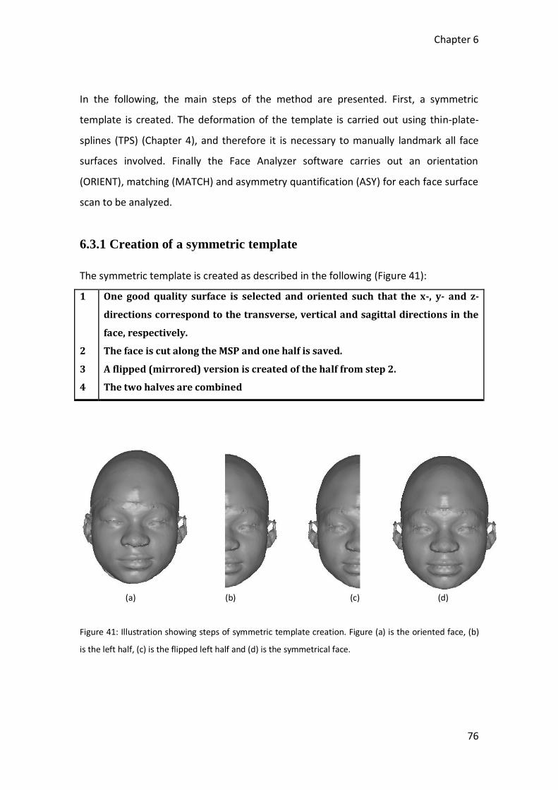
Chapter 6
76
In the following, the main steps of the method are presented. First, a symmetric
template is created. The deformation of the template is carried out using thin-plate-
splines (TPS) (Chapter 4), and therefore it is necessary to manually landmark all face
surfaces involved. Finally the Face Analyzer software carries out an orientation
(ORIENT), matching (MATCH) and asymmetry quantification (ASY) for each face surface
scan to be analyzed.
6.3.1 Creation of a symmetric template
The symmetric template is created as described in the following (Figure 41):
1
2
3
4
One good quality surface is selected and oriented such that the x-, y- and z-
directions correspond to the transverse, vertical and sagittal directions in the
face, respectively.
The face is cut along the MSP and one half is saved.
A flipped (mirrored) version is created of the half from step 2.
The two halves are combined
(a) (b) (c) (d)
Figure 41: Illustration showing steps of symmetric template creation. Figure (a) is the oriented face, (b)
is the left half, (c) is the flipped left half and (d) is the symmetrical face.

Chapter 6
77
The symmetric template has a number of landmark points associated with it (see
Figure 42). The landmarks are also located fully symmetrically in the face. This is
achieved by carefully landmarking the left side of the face, and subsequently these
landmarks are flipped across the MSP (x=0.0) to create the landmarks on the right side.
Landmarks in the midline (e.g. nasion, tip of the nose, chin) are carefully placed,
followed by a small correction of their coordinates in order for them to be located
exactly at x=0.0.
Figure 42: The symmetric template and the symmetric point landmarks associated with it. 25 landmarks
are used in this case.
The wide face used later for the validation is created in the same way as the symmetric
template. After cutting along the MSP a flipped (mirrored) version is made. The flipped
surface scan is then stretched (in this study the face is stretched 1.2, 1.4 and 1.6 mm)
by means of the software program Landmarker (previously developed at the 3D
Craniofacial Image Research Laboratory). Subsequently the two halves are combined.
For an optimal deformation of the template to assume the shape of the subject
surface scan, the template shape should be as similar as possible to the subject shape

Chapter 6
78
under study. However, since the method requires that the same template is used for
matching to all the surface scans in a group, a template representing the group mean
shape would be expected to be an optimal choice. Before the matching, the surface
scans and the landmarks are oriented to the template surface using rigid
transformation, involving translation and rotation.
In practice, we build such a mean shape (also termed atlas) and create a (mean)
symmetric template by the same steps as shown in Figure 41. This symmetric
template, based on the mean shape, is then used in the subsequent asymmetry
quantification.
A template was made as the mean of all scans (the 10 African American boys), which is
an optimal choice as described above.
6.3.2 Landmarking
Before the orientation, matching and asymmetry quantification takes place, each facial
surface scan needs to be manually landmarked. This is carried out in the software
program Landmarker (Darvann 2008). It allows easy landmarking in 3D by pointing out
locations of interest on a surface rendering using the computer mouse. The surface
may be interactively zoomed, panned and rotated during landmarking, and landmark
positions may be, among other things, easily reviewed, edited, saved and reloaded.
The landmarks are set at anatomical locations in the faces. It was noted that the
number and location of the landmarks influence the result of the asymmetry
quantification. Therefore, a number of experiments were carried out to clarify this.
In the first experiment, 26 landmarks are set on each surface scan (red spheres; see
Figure 42). The landmarks are placed at the anatomical locations by looking at the
whole face. The localization of landmarks at one side of MSP can depend on the

Chapter 6
79
opposite side of MSP. This fact can introduce an error from the true value since the
amount of asymmetry can be different when consideration of both sides of the face is
taken.
In the second experiment, 26 landmarks are again set on each surface scan. This time,
the landmark localization is carried out by only looking at one half of the face (right or
left side of MSP). The assumption is that the landmarks will be placed more correctly
(on the anatomical structure), since consideration of the opposite side of the face is
not taken into account. This will, perhaps, induce that the landmarks are set exactly on
the anatomical location of the face and thereby reduce error induced by looking at the
whole face.
In the third and fourth experiment 6 and 19 landmarks are set respectively to see how
the number of landmarks impacts the result of asymmetry quantification.
6.3.3 Orient
Each surface scan is oriented to the template surface by use of rigid transformation
using all landmarks. The result is translated such that the midpoint between ear
landmarks for the surface scan and the template coincide.
6.3.4 Match
Following the orientation of the scan to the template, the template is scaled to the size
of the scan. Subsequently, the template is deformed using TPS (Thin-Plate Splines)
(controlled by landmarks) and CP (closest point deformation) (Chapter 4).
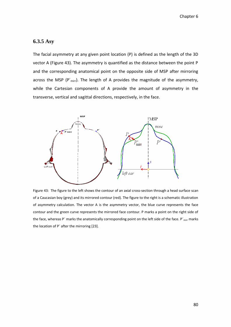
Chapter 6
80
6.3.5 Asy
The facial asymmetry at any given point location (P) is defined as the length of the 3D
vector A (Figure 43). The asymmetry is quantified as the distance between the point P
and the corresponding anatomical point on the opposite side of MSP after mirroring
across the MSP (P´mirr). The length of A provides the magnitude of the asymmetry,
while the Cartesian components of A provide the amount of asymmetry in the
transverse, vertical and sagittal directions, respectively, in the face.
Figure 43: The figure to the left shows the contour of an axial cross-section through a head surface scan
of a Caucasian boy (grey) and its mirrored contour (red). The figure to the right is a schematic illustration
of asymmetry calculation. The vector A is the asymmetry vector, the blue curve represents the face
contour and the green curve represents the mirrored face contour. P marks a point on the right side of
the face, whereas P´ marks the anatomically corresponding point on the left side of the face. P´mirr marks
the location of P´ after the mirroring [23].
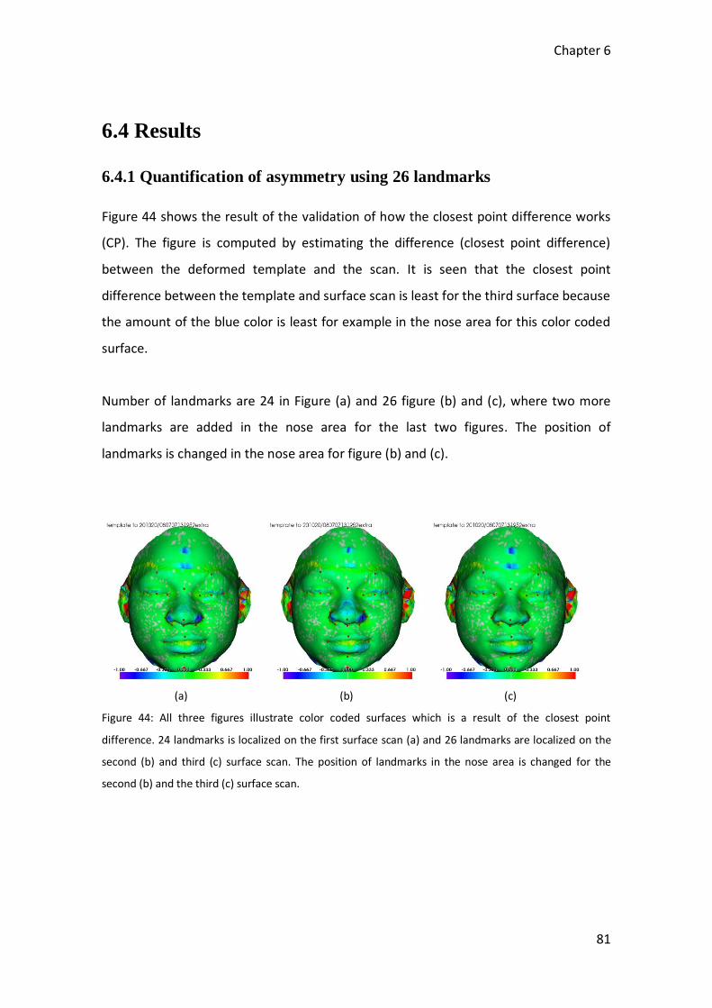
Chapter 6
81
6.4 Results
6.4.1 Quantification of asymmetry using 26 landmarks
Figure 44 shows the result of the validation of how the closest point difference works
(CP). The figure is computed by estimating the difference (closest point difference)
between the deformed template and the scan. It is seen that the closest point
difference between the template and surface scan is least for the third surface because
the amount of the blue color is least for example in the nose area for this color coded
surface.
Number of landmarks are 24 in Figure (a) and 26 figure (b) and (c), where two more
landmarks are added in the nose area for the last two figures. The position of
landmarks is changed in the nose area for figure (b) and (c).
(a) (b) (c)
Figure 44: All three figures illustrate color coded surfaces which is a result of the closest point
difference. 24 landmarks is localized on the first surface scan (a) and 26 landmarks are localized on the
second (b) and third (c) surface scan. The position of landmarks in the nose area is changed for the
second (b) and the third (c) surface scan.

Chapter 6
82
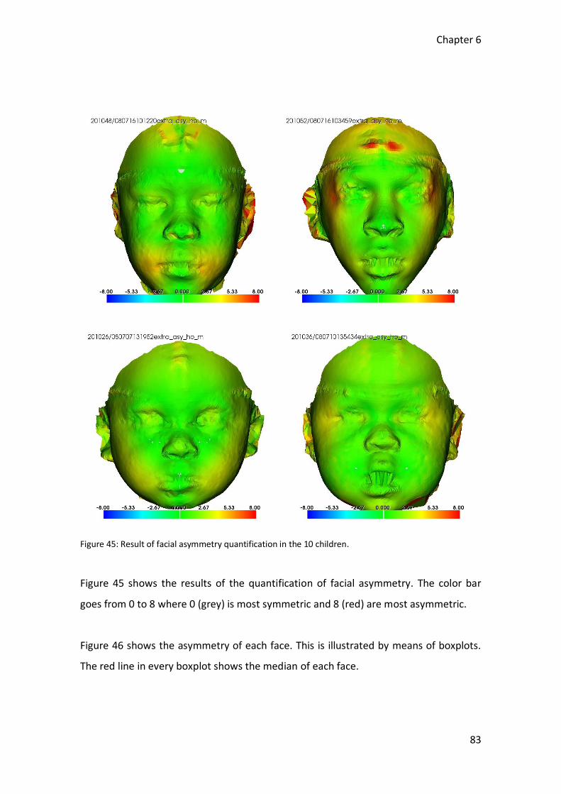
Chapter 6
83
Figure 45: Result of facial asymmetry quantification in the 10 children.
Figure 45 shows the results of the quantification of facial asymmetry. The color bar
goes from 0 to 8 where 0 (grey) is most symmetric and 8 (red) are most asymmetric.
Figure 46 shows the asymmetry of each face. This is illustrated by means of boxplots.
The red line in every boxplot shows the median of each face.
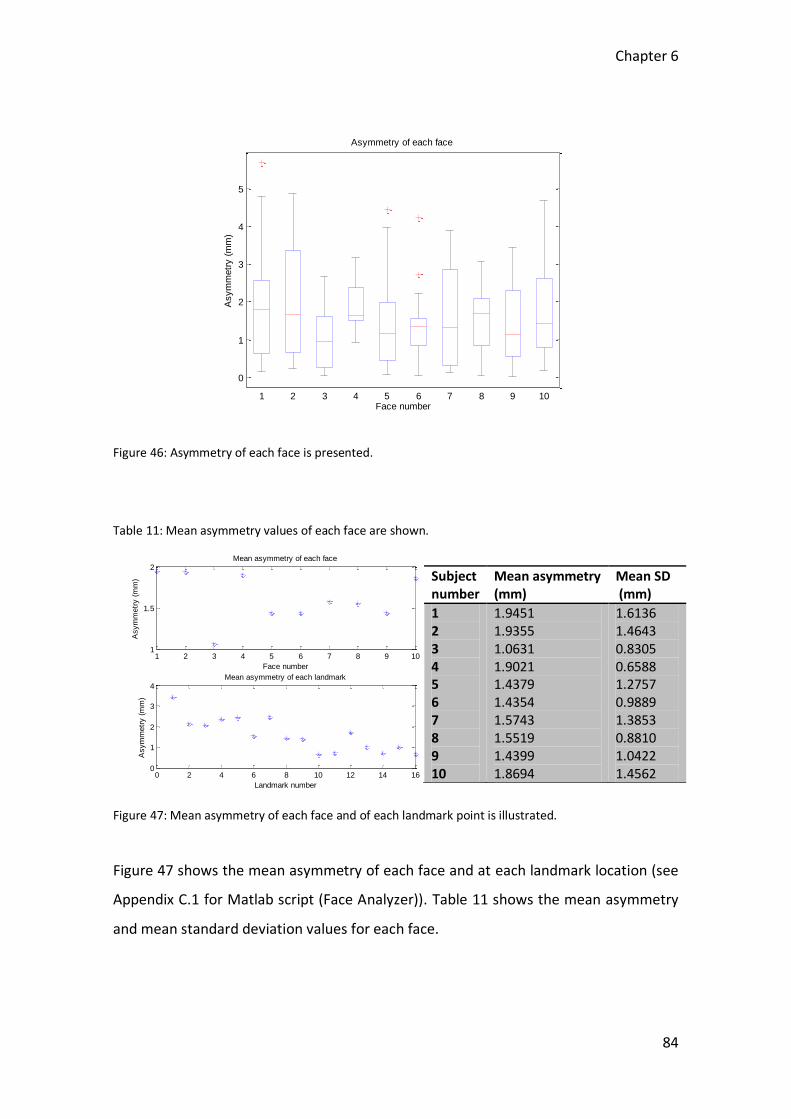
Chapter 6
84
Figure 46: Asymmetry of each face is presented.
Table 11: Mean asymmetry values of each face are shown.
Figure 47: Mean asymmetry of each face and of each landmark point is illustrated.
Figure 47 shows the mean asymmetry of each face and at each landmark location (see
Appendix C.1 for Matlab script (Face Analyzer)). Table 11 shows the mean asymmetry
and mean standard deviation values for each face.
0
1
2
3
4
5
1 2 3 4 5 6 7 8 9 10Face number
Asym
metr
y (
mm
)
Asymmetry of each face
1 2 3 4 5 6 7 8 9 101
1.5
2
Face number
Asym
metr
y (
mm
)
Mean asymmetry of each face
0 2 4 6 8 10 12 14 160
1
2
3
4
Landmark number
Asym
metr
y (
mm
)
Mean asymmetry of each landmark
Subject number
Mean asymmetry (mm)
Mean SD (mm)
1 2 3 4 5 6 7 8 9 10
1.9451 1.9355 1.0631 1.9021 1.4379 1.4354 1.5743 1.5519 1.4399 1.8694
1.6136 1.4643 0.8305 0.6588 1.2757 0.9889 1.3853 0.8810 1.0422 1.4562
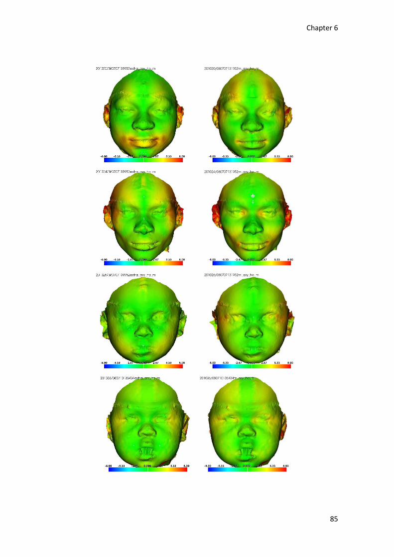
Chapter 6
85

Chapter 6
86

Chapter 6
87
Figure 48: The figures to the left shows the result of the landmarks set by looking at the whole face and
the figures to the right shows the result of the face when setting landmarks only by looking at one side
of the face.

Chapter 6
88
Figure 48 illustrates that the method is sensitive with respect to the landmarking. The
surfaces in the left column shows the result of landmarking by looking at the whole
face and the figures in the right column shows the result of landmarking by only
looking at one side of the face. The surfaces to the right seem to be more asymmetric
because it contains more of the red color especially in the eye and mouth area.
Figure 49 shows the mean facial asymmetry for 10 faces. The red points are the result
of mean facial asymmetry of landmarking by looking at the whole face and the green
points are the result of facial asymmetry of landmarking by only looking at one side of
the face.
Figure 49: Mean facial asymmetry for the faces by two different landmarking processes. The red points
are mean facial asymmetry when landmarking by looking at the whole face and the green points are
facial asymmetry when landmarking by only looking at one side of the face.
1 2 3 4 5 6 7 8 9 101
1.2
1.4
1.6
1.8
2
2.2
2.4
2.6
2.8
3
Face number
Mean a
sym
metr
y
Mean asymmetry of faces by two difference landmarking processes
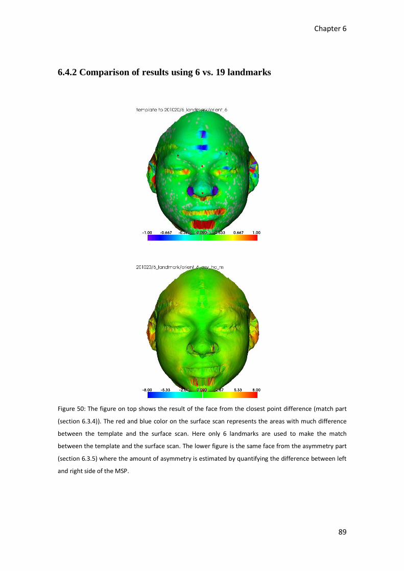
Chapter 6
89
6.4.2 Comparison of results using 6 vs. 19 landmarks
Figure 50: The figure on top shows the result of the face from the closest point difference (match part
(section 6.3.4)). The red and blue color on the surface scan represents the areas with much difference
between the template and the surface scan. Here only 6 landmarks are used to make the match
between the template and the surface scan. The lower figure is the same face from the asymmetry part
(section 6.3.5) where the amount of asymmetry is estimated by quantifying the difference between left
and right side of the MSP.
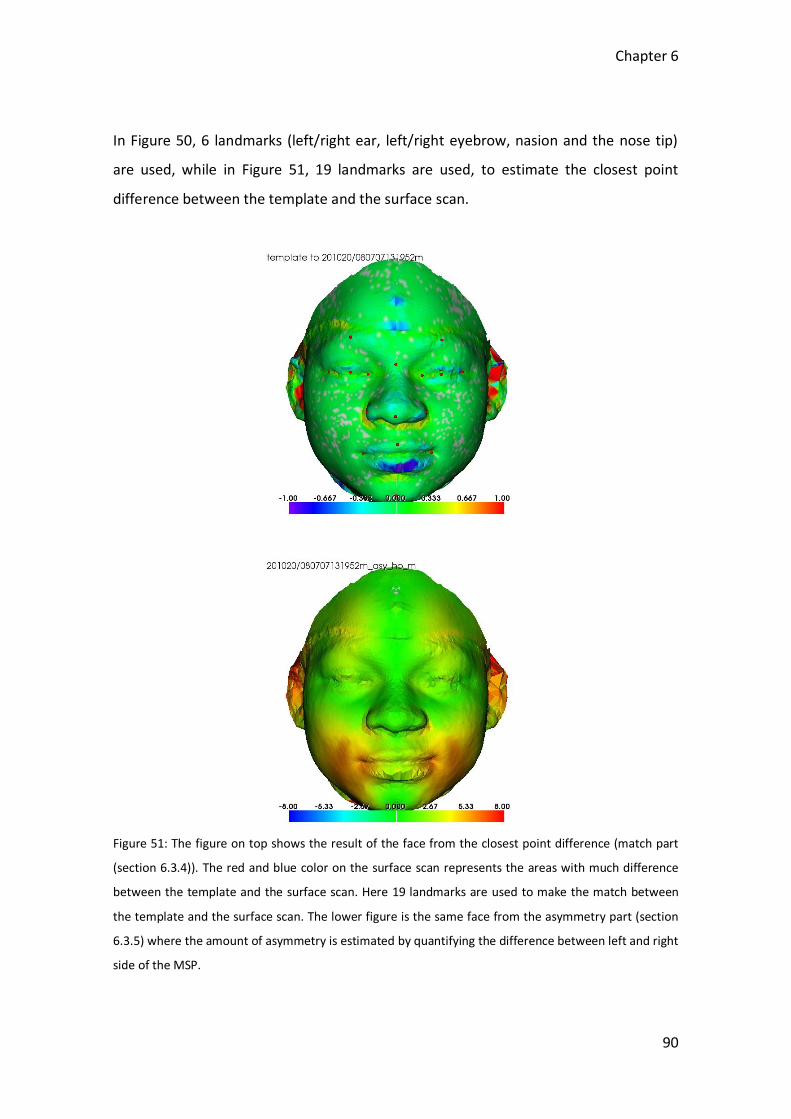
Chapter 6
90
In Figure 50, 6 landmarks (left/right ear, left/right eyebrow, nasion and the nose tip)
are used, while in Figure 51, 19 landmarks are used, to estimate the closest point
difference between the template and the surface scan.
Figure 51: The figure on top shows the result of the face from the closest point difference (match part
(section 6.3.4)). The red and blue color on the surface scan represents the areas with much difference
between the template and the surface scan. Here 19 landmarks are used to make the match between
the template and the surface scan. The lower figure is the same face from the asymmetry part (section
6.3.5) where the amount of asymmetry is estimated by quantifying the difference between left and right
side of the MSP.

Chapter 6
91
6.4.3 Validation
A way of validating the method is to apply it to faces exhibiting known amounts of
asymmetry. In this section the method is validated by applying it to different artificially
created face surfaces:
1. A fully symmetric surface (the method should provide 0.0 mm asymmetry
everywhere) and
2. Three surfaces with known amounts of asymmetry. The surfaces were created
by stretching (scaling in the x-direction) the left side of the symmetric face.
Figure 52 shows the symmetric face created as explained in section 6.3.1. The color
coding of the surface in Figure 52 indicates the amount and spatial distribution of
calculated asymmetry. Figure 53 shows three “stretched” faces. The left side of the
faces (a), (b) and (c) are scaled by a factor 1.2, 1.4, and 1.6, respectively.
Figure 52: Artificially created symmetric face. The colors represent the amount of asymmetry in the face
as quantified by the developed method. The face is grey if the asymmetry values are close to zero which
indicates it is symmetrical.

Chapter 6
92
(a) (b) (c)
Figure 53: Figure (a) a face stretched 1.2 mm. Figure (b) a face stretched 1.4 mm and Figure (c) a face
stretched 1.6 mm.
6.4.4 Comparison between the method presented in the current
chapter and the method of Chapter 5
Table 12 shows the mean asymmetry values for each landmark location using the
landmark based methods presented in the current chapter and in Chapter 5,
respectively.
It is seen that most of the asymmetry values are almost identical for the landmark
locations when comparing the two methods. Only the landmark for the eyebrow
(landmark number 3) has a little deviation which depends on eyebrow correction used
in the software program Face Analyzer. Therefore the results of these landmarks
should be discarded when the comparison is made.

Chapter 6
93
Table 12: The amount of asymmetry for each landmark location using the two methods
Landmark number Landmark based method (current chapter)
Landmark based method (Chapter 5)
1 2 3 4 5 6 7 8 9 10 11
3.7757 2.3318 1.6064 3.7715 2.5714 1.3152 2.6635 0.9172 0.8936 1.1539 1.2700
3.7513 2.3842 2.4602 3.8046 2.6391 1.3967 2.6794 0.9244 0.8971 1.1482 1.2678
Figure 54 shows the amount of asymmetry for each subject for the two methods
(method presented in Chapter 5 and method presented in current chapter). The
asymmetry is shown as points where the blue color represent the facial asymmetry for
the method presented in current chapter and the red color represent the facial
asymmetry for the method presented in Chapter 5.
Figure 55 shows the amount of asymmetry for the two methods plotted against each
other where a relation is studied between these two methods (see Appendix A.1 for
the other landmark locations).
The figures show a very good correspondence between the methods.

Chapter 6
94
Figure 54: The amount of asymmetry for each subject for the landmark based method presented in the
current chapter (blue) and Chapter 5 (red) is seen as points. The plot to the left shows the amount of
asymmetry for the eye center landmark while the plot to the right shows the amount of asymmetry for
the nasion landmark.
Figure 55: The amount of asymmetry for the landmark based method presented in the current chapter
and in Chapter 5 is plotted against each other. The plot to the left shows the asymmetry for the eye
center landmark while the plot to the right shows the asymmetry for the nasion landmark.
0 5 10 15 20 25 300
1
2
3
4
5
6
7
8
Face number
Asym
metr
y (
mm
)Asymmetry value for landmark of the eye center for each face for the two methods
0 5 10 15 20 25 300
0.5
1
1.5
2
2.5
3
3.5
Face number
Asym
metr
y (
mm
)
Asymmetry value for landmark of the nasion for each face for the two methods
0 1 2 3 4 5 6 7 80
1
2
3
4
5
6
7
8
9
Asymmetry (mm) (method presented in Chapter 5)
Asym
metr
y (
mm
)(m
eth
od p
resente
d in C
hapte
r 6)
Asymmetry of the eye center for landmark based method
0 0.5 1 1.5 2 2.5 3 3.50
0.5
1
1.5
2
2.5
3
3.5
Asymmetry (mm) (method presented in Chapter 5)
Asym
metr
y (
mm
)(m
eth
od p
resente
d in C
hapte
r 6)
Asymmetry of the nasion for landmark based method
Chapter 6
95
6.5 Discussion and Conclusion
6.5.1 Asymmetry in 10 African American boys
Figure 45 shows 10 different color coded surfaces where the amount of asymmetry is
indicated by the color. The area of the surfaces containing the green color indicates
less asymmetry while red areas indicate more asymmetry. In terms of mean facial
asymmetry, the amount of asymmetry does not vary much between the different
faces. This is also demonstrated in Figure 46 which shows the amount of asymmetry of
each face by means of boxplots, even though there is a considerable contribution from
landmark-void areas (forehead and neck) and noise-filled areas (ears) that could have
been masked out from the computation.
Figure 47 shows the mean asymmetry of each face and the mean asymmetry at each
landmark location. The asymmetry values in the table next to Figure 47 show that the
mean amount of asymmetry in each face is quite similar. The mean asymmetry value
of these 10 African American boys is 1.62 mm. This value indicates that the amount of
asymmetry is small in these boys.
However, when looking at the spatial distribution of asymmetry across the facial
surfaces of different individuals, these are all very different. It is difficult to find any
typical pattern of asymmetry in the population. This is as would be expected in a
normal healthy group of individuals: by a combination of genetic and environmental
factors, their patterns of facial asymmetry have become all different.
6.5.2 Landmarking by looking at one side of the face and at the whole
face
This experiment is implemented for 10 faces and 8 out of these 10 faces showed that
the amount of facial asymmetry increases when landmarking happens by only looking

Chapter 6
96
at one side of the face. This is also seen in Figure 49 which shows the mean facial
asymmetry for each face by a red (when landmarking by looking at the whole face) and
green (when landmarking by only looking at one side of the face) color.
By looking at Figure 48 it can be stated that the amount of asymmetry increases when
landmarking happens by only looking at one side of the face. This result can of course
also depend on other factors because the amount of facial asymmetry can change for
every landmarking processes, and therefore it is important to implement this
experiment for several subjects to make a conclusion.
6.5.3 The importance of position of landmarks
Number and position of landmarks are also an important factor when amount of
asymmetry is studied. Figure 44 shows three match figures of the same face. As
shown, the last (c) figure is the best of all tree figures (least blue color in nose area)
since the closest point difference between the template and the surface scan is least
for that experiment, where number and position of landmarks are changed.
This indicates that the position and numbers of landmarks are very important, since a
better result is achieved.
6.5.4 The importance of number of landmarks
In the attempt to find the asymmetry by only using 6 landmarks, the result became
much poorer. This is very well illustrated in Figure 50. The figure from the match part
(the result of closest point difference between the template and the surface scan)
shows drastic colors (indicating bad match due to lack of landmark guidance for the
TPS and CP transformations) and the figure illustrating the asymmetry clearly shows
that the amount of asymmetry is much higher (compared to for example Figure 45).
This clearly indicates that too few landmarks lead to poor results of asymmetry.
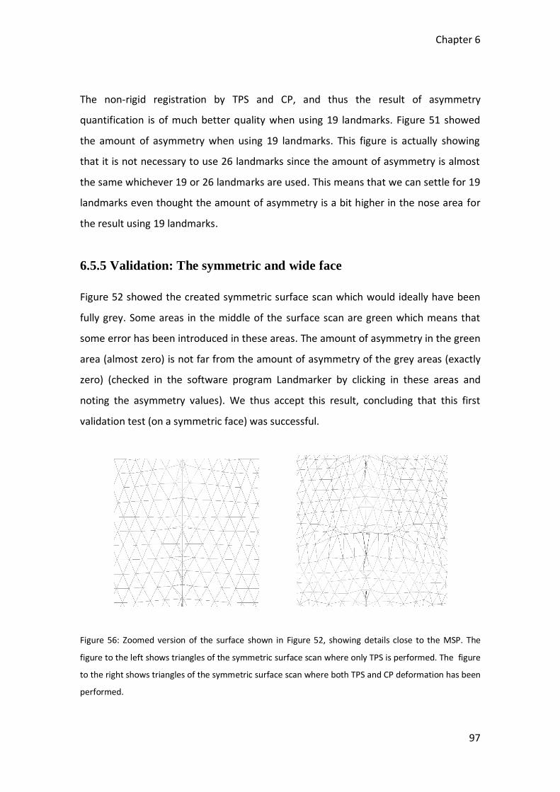
Chapter 6
97
The non-rigid registration by TPS and CP, and thus the result of asymmetry
quantification is of much better quality when using 19 landmarks. Figure 51 showed
the amount of asymmetry when using 19 landmarks. This figure is actually showing
that it is not necessary to use 26 landmarks since the amount of asymmetry is almost
the same whichever 19 or 26 landmarks are used. This means that we can settle for 19
landmarks even thought the amount of asymmetry is a bit higher in the nose area for
the result using 19 landmarks.
6.5.5 Validation: The symmetric and wide face
Figure 52 showed the created symmetric surface scan which would ideally have been
fully grey. Some areas in the middle of the surface scan are green which means that
some error has been introduced in these areas. The amount of asymmetry in the green
area (almost zero) is not far from the amount of asymmetry of the grey areas (exactly
zero) (checked in the software program Landmarker by clicking in these areas and
noting the asymmetry values). We thus accept this result, concluding that this first
validation test (on a symmetric face) was successful.
Figure 56: Zoomed version of the surface shown in Figure 52, showing details close to the MSP. The
figure to the left shows triangles of the symmetric surface scan where only TPS is performed. The figure
to the right shows triangles of the symmetric surface scan where both TPS and CP deformation has been
performed.
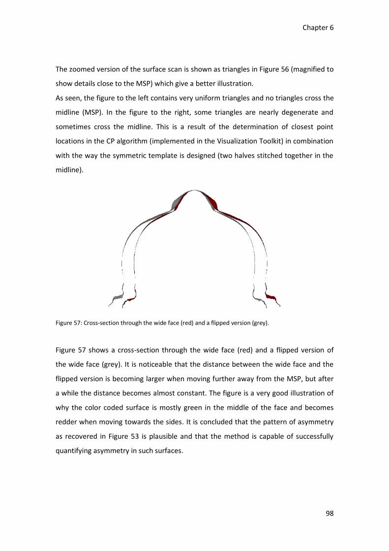
Chapter 6
98
The zoomed version of the surface scan is shown as triangles in Figure 56 (magnified to
show details close to the MSP) which give a better illustration.
As seen, the figure to the left contains very uniform triangles and no triangles cross the
midline (MSP). In the figure to the right, some triangles are nearly degenerate and
sometimes cross the midline. This is a result of the determination of closest point
locations in the CP algorithm (implemented in the Visualization Toolkit) in combination
with the way the symmetric template is designed (two halves stitched together in the
midline).
Figure 57: Cross-section through the wide face (red) and a flipped version (grey).
Figure 57 shows a cross-section through the wide face (red) and a flipped version of
the wide face (grey). It is noticeable that the distance between the wide face and the
flipped version is becoming larger when moving further away from the MSP, but after
a while the distance becomes almost constant. The figure is a very good illustration of
why the color coded surface is mostly green in the middle of the face and becomes
redder when moving towards the sides. It is concluded that the pattern of asymmetry
as recovered in Figure 53 is plausible and that the method is capable of successfully
quantifying asymmetry in such surfaces.

99
6.5.6 Validation of landmark based method
When comparing the method present in current chapter and the method present in
Chapter 5, it is seen that the result of asymmetry is almost equal (see Table 12 and
Figure 54 and 55). This result successfully validates the implementation of the method
as used in the present chapter.

100
Chapter 7
101
Chapter 7
Automatic quantification of facial
asymmetry using non-rigid surface
registration
7.1 Introduction
Asymmetry quantification involves a comparison between opposite sides of the face,
and thus corresponding anatomical structures on the right and left side, respectively,
must be located. In Chapter 6, spatially dense left-right correspondences (i.e.
everywhere across the face) were established by deforming a symmetric face template
to each face (modeled by TPS and CP transformation) under study. The deformation
was guided by manually placed landmarks. The method in Chapter 6 may thereby be
categorized as being spatially detailed, landmark based and guided (i.e. requires
manual input).
However, manual landmark placement is time consuming and has a finite
reproducibility as shown in Chapter 5. Therefore, replacing the manual landmarking by
a method that could establish dense point correspondence between left and right
sides of the face would potentially be of great advantage.
In the present chapter, the non-rigid surface registration method by Szeliski and
Lavallée [26] is used as an automatic means of establishing left-right correspondence.
We use the implementation made available through the Image Registration Toolkit
Chapter 7
102
[36] which is a freely downloaded resource on the internet, developed by Daniel
Rueckert at Imperial College, London, England. While the method is usually applied in
order to achieve non-rigid registration between two (similar) surfaces (e.g. faces), we
use it for non-rigid registration of a face to its mirrored version. This alternative
method of asymmetry quantification thus becomes, as we shall see, spatially detailed,
surface based and automatic.
Validation of method is carried out by comparing the calculated asymmetry values at a
number of anatomical landmark locations to the asymmetry obtained by direct
landmarking of the same surfaces as used in Chapter 5.
7.2 Material
The material consisted of surface scans of 29 normal children. These are a subset of
the 30 surface scans used in Chapter 5. One scan had to be removed from the analysis
due to incomplete data. The facial surface scans represented children of different ages,
gender and ethnicity (Section 5.2 in Chapter 5).
Manually placed landmarks are anatomically localized on the face surfaces for the
purpose of implementing an orientation before asymmetry estimation. Also, the
landmarks are used for the validation purposes.
7.3 Method
The goal of this chapter is to develop a method that quantifies the facial asymmetry
automatically using non-rigid surface registration. It was defined in Chapter 3 that
asymmetry is the difference between geometry on the left and right side of the face.

Chapter 7
103
This means that the method should require an establishment of detailed point
correspondence between surface points on the left and right side of the MSP.
Figure 58 illustrates the main steps of the method. First, each of the 29 3D surface
scans will be oriented (1. in Figure 58) in the framework of a software program called
Face Analyzer previously developed at the 3D Craniofacial Image Research Laboratory.
Before the orientation of the surface scans, manually placed landmarks will be used
(landmarks are anatomically localized on the face surfaces). Landmark localization is
needed since the orientation uses rigid landmark based transformation.
Subsequently, the surface scans are flipped (mirrored across the MSP; 2. in Figure 58)
and then the flipped version of the surface scans will be deformed to have the same
shape as the original surface scans using non-rigid registration (3. in Figure 58). Finally,
the vector A between the flipped and the deformed (original) surface scan is calculated
in every surface point, representing asymmetry. The steps will be explained in greater
detail in the following sections.
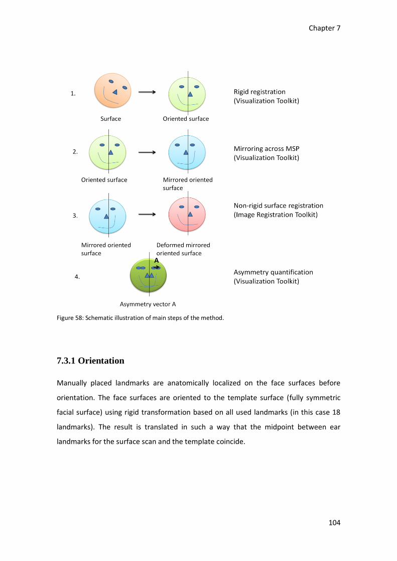
Chapter 7
104
Figure 58: Schematic illustration of main steps of the method.
7.3.1 Orientation
Manually placed landmarks are anatomically localized on the face surfaces before
orientation. The face surfaces are oriented to the template surface (fully symmetric
facial surface) using rigid transformation based on all used landmarks (in this case 18
landmarks). The result is translated in such a way that the midpoint between ear
landmarks for the surface scan and the template coincide.

Chapter 7
105
Figure 59: The figure to the left is the original surface scan (grey) and the flipped surface scan (yellow)
on top of each other. The figure to the right is the result of the iterated closest point alignment where
the flipped surface scan is rigidly registered to the original surface scan.
There are another methods that could also be used for the orientation step, e.g. the
iterated closest point (ICP) alignment where the flipped surface scan is transformed to
the original surface scan (see to the right in Figure 59). This method (ICP) is not used in
the current chapter due to the noise circumstances (holes, spikes and variables
amounts of neck and shoulder in scans).
7.3.2 Flipping
After orientation the surface scans are flipped (left-right reflection). This is
implemented by writing a tcl script calling procedures available through the software
program Landmarker (Darvann 2008). A flipped surface scan is seen to the right in
Figure 60.

Chapter 7
106
Figure 60: 3D surface scan of a boy. The figure to the left is the orientated original surface scan while the
figure to the right is the flipped version of the oriented original surface scan.
7.3.3 Deformation/matching
This step has the same purpose of the match part (see section 6.3.4) in Chapter 6 but
the implementation is different in the current chapter. In contrast to the method
presented in Chapter 6, where the match was found between a surface scan and a
symmetric template, the match in the current chapter is achieved by non-rigid
registration of two surfaces (the original surface scan and the flipped version of the
original surface scan) using the method of Szeliski and Lavallée [26] which is available
as one of the programs in the Image Registration Toolkit [36] (see Figure 61 for a series
of iterations of non-rigid deformation).
The deformation is described as a warping of the space containing one of the surfaces.
The intention is to bring the two surfaces into registration, while maintaining
smoothness and avoiding unnecessary quantification. The registration is rapid and
efficient and does not require extraction (manual or automatic) of features on the two
surfaces. The registration can be used on randomly shaped surfaces and with highly
complicated deformations [26].

Chapter 7
107
Figure 61: The figures show subsequently iterations of non-rigid deformation where the first figure is the
result of the first iteration and the last figure is the result of the last iteration.
7.3.4 Difference
The purpose of this step is to calculate the vector A (4. in Figure 58) between
corresponding points in two surfaces. The mentioned two surfaces are the flipped
surface scan and the deformed surface scan (3. in Figure 58). The asymmetry at every
surface point is stored in color files and used in order to illustrate the amount of
asymmetry by means of color coded surfaces.
Below, the amount of the asymmetry is seen for one child by means of color coded
surfaces. Figure 62 (a) shows the amount (magnitude) of asymmetry, while figure (b),
(c) and (d) show the amount of asymmetry in the transverse, vertical and sagittal
planes, respectively.
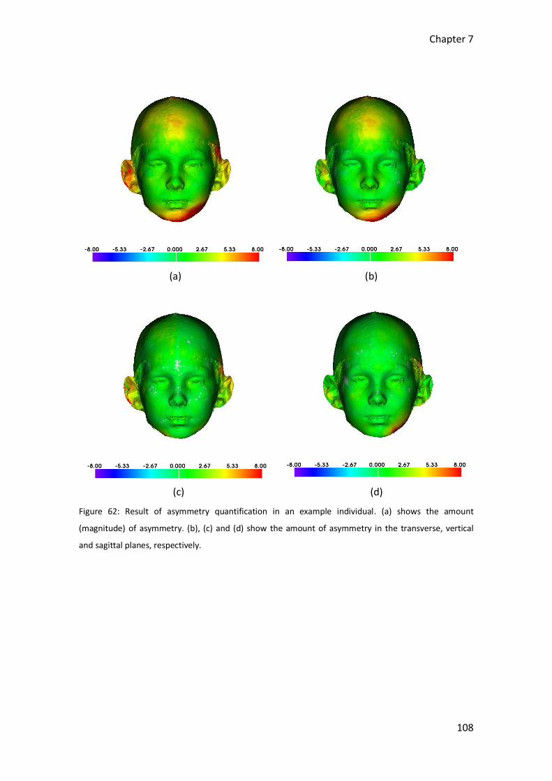
Chapter 7
108
(a) (b)
(c) (d)
Figure 62: Result of asymmetry quantification in an example individual. (a) shows the amount
(magnitude) of asymmetry. (b), (c) and (d) show the amount of asymmetry in the transverse, vertical
and sagittal planes, respectively.
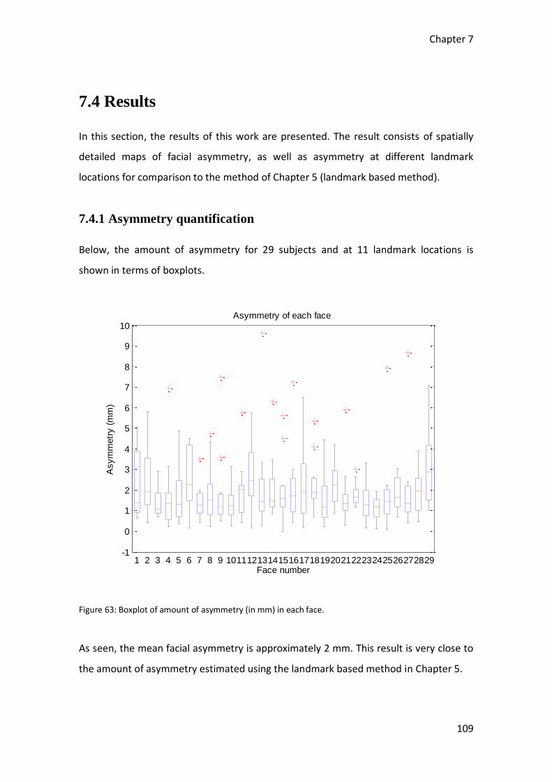
Chapter 7
109
7.4 Results
In this section, the results of this work are presented. The result consists of spatially
detailed maps of facial asymmetry, as well as asymmetry at different landmark
locations for comparison to the method of Chapter 5 (landmark based method).
7.4.1 Asymmetry quantification
Below, the amount of asymmetry for 29 subjects and at 11 landmark locations is
shown in terms of boxplots.
Figure 63: Boxplot of amount of asymmetry (in mm) in each face.
As seen, the mean facial asymmetry is approximately 2 mm. This result is very close to
the amount of asymmetry estimated using the landmark based method in Chapter 5.
-1
0
1
2
3
4
5
6
7
8
9
10
1 2 3 4 5 6 7 8 9 1011121314151617181920212223242526272829Face number
Asym
metr
y (
mm
)
Asymmetry of each face

Chapter 7
110
Figure 64 shows the amount of asymmetry in each landmark location. A larger
variation and a larger amount of asymmetry in landmark number 1 (landmark of the
ear) and landmark number 11 (landmark of the chin) can be seen.
Figure 64: Boxplot of amount of asymmetry (in mm) in each landmark location.
Figure 65 and 66 shows the asymmetry values for the mean, standard deviation,
maximum and minimum for each face and for each landmark location, respectively.
-1
0
1
2
3
4
5
6
7
8
9
10
1 2 3 4 5 6 7 8 9 10 11Landmark number
Asym
metr
y (
mm
)
Asymmetry for each landmark location

Chapter 7
111
Figure 65: Plots of mean-, standard deviation-, maximum- and minimum asymmetry values of each face.
Figure 66: Illustration of mean-, standard deviation-, maximum- and minimum asymmetry values of each
landmark point.
0 10 20 301
2
3
4
Face
Asym
metr
y (
mm
)
Mean
0 10 20 300
1
2
3
Face
Asym
metr
y (
mm
)
Standard deviation
0 10 20 300
5
10
Face
Asym
metr
y (
mm
)
Maximum value
0 10 20 300
0.5
1
1.5
Face
Asym
metr
y (
mm
)
Minimum value
0 5 101
2
3
4
5
Landmark number
Asym
metr
y (
mm
)
Mean
0 5 100
1
2
3
Landmark number
Asym
metr
y (
mm
)
Standard deviation
0 5 102
4
6
8
10
Landmark number
Asym
metr
y (
mm
)
Maximum value
0 5 100
0.5
1
1.5
Landmark number
Asym
metr
y (
mm
)
Minimum value

Chapter 7
112
Figure 67 shows the results of the facial asymmetry quantification for some of the
individuals. The figure consists of color coded surfaces where the color bar goes from 0
to 8 mm where 0 (grey) is symmetric and 8 (red) is most asymmetric.
(a) (b)
(c) (d)

Chapter 7
113
(e) (f)
(g) (h)
Figure 67: Result of facial asymmetry quantification in 8 individuals. (a) and (b): Caucasian boys of age 9
and 13 years, respectively. (c) and (d): African American boys of age 12 and 17 years, respectively. (e)
and (f): Caucasian girls of age 9 and 2 years, respectively. (g) and (h): African American girls of age 7 and
11 years, respectively.
7.4.2 Comparison between surface and landmark based method
Table 13 shows the mean facial asymmetry for each subject using the surface based
method and the landmark based method, respectively. Table 14 shows the mean
asymmetry value for each landmark location using the two methods.

Chapter 7
114
Table 13: Mean facial asymmetry for each subject using the surface based method and the landmark
based method, respectively.
Landmark number
Surface based method
Landmark based method
1 2 3 4 5 6 7 8 9 10 11 12 13 14 15 16 17 18 19 20 21 22 23 24 25 26 27 28 29
2.2325 2.4794 1.3779 1.7557 1.7343 2.6112 1.4808 1.8696 1.8966 1.4330 1.9676 2.6653 2.2606 2.0931 2.0187 2.0905 2.3106 2.3589 1.5269 2.2312 1.7043 1.7880 1.3924 1.1120 1.8464 1.8895 2.0686 1.8910 3.0510
2.0989 2.2365 1.3090 1.9685 1.8182 1.6123 1.9199 1.7188 1.5275 2.0727 2.0931 3.0342 2.1239 2.4396 1.9210 2.4071 2.7252 2.0041 2.3052 2.3211 3.1989 2.0543 2.6521 1.7935 1.6193 2.3982 1.6885 1.9976 2.2281
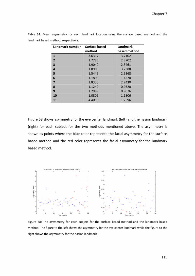
Chapter 7
115
Table 14: Mean asymmetry for each landmark location using the surface based method and the
landmark based method, respectively.
Landmark number Surface based method
Landmark based method
1 2 3 4 5 6 7 8 9 10 11
3.6317 1.7783 1.9042 1.8903 1.5446 1.1808 1.8336 1.1242 1.2989 1.0809 4.4053
3.7102 2.3702 2.3461 3.7388 2.6368 1.4220 2.7430 0.9320 0.9076 1.1806 1.2596
Figure 68 shows asymmetry for the eye center landmark (left) and the nasion landmark
(right) for each subject for the two methods mentioned above. The asymmetry is
shown as points where the blue color represents the facial asymmetry for the surface
based method and the red color represents the facial asymmetry for the landmark
based method.
Figure 68: The asymmetry for each subject for the surface based method and the landmark based
method. The figure to the left shows the asymmetry for the eye center landmark while the figure to the
right shows the asymmetry for the nasion landmark.
0 5 10 15 20 25 300
1
2
3
4
5
6
7
8
Face number
Asym
metr
y (
mm
)
Asymmetry for surface and landmark based method
0 5 10 15 20 25 300
0.5
1
1.5
2
2.5
3
3.5
4
4.5
Face number
Asym
metr
y (
mm
)
Asymmetry for surface and landmark based method

Chapter 7
116
Figure 69 shows the asymmetry for the above mentioned landmark locations for the
two methods plotted against each other (see Appendix A.2 for the other landmark
locations).
Figure 69: The amount of asymmetry for the surface based method and landmark based method plotted
against each other. The figure to the left shows the amount of asymmetry for the eye center landmark
while the figure to the right shows the amount of asymmetry for the nasion landmark.
7.5 Discussion and Conclusion
7.5.1 Asymmetry quantification
In this chapter, a well-functioning framework for asymmetry quantification (Figure 58)
has been established, where an automatic, surfaced based non-rigid registration
technique was used for the establishment of left-right point correspondence.
The method provided an overall facial asymmetry of approximately 2 mm (Figure 63
and 64), which seemingly confirmed the result of the landmark-guided method of
Chapter 5. The method was able to provide detailed maps of facial asymmetry (Figure
62 and 67), as well as statistics (mean, SD, minimum and maximum) of asymmetry for
each face and at particular landmark locations (Figures 63-66).
0 1 2 3 4 5 6 7 80
0.5
1
1.5
2
2.5
3
3.5
4
4.5
Asymmetry (landmark based method)
Asym
metr
y (
auto
matic m
eth
od)
Asymmetry for surface and landmark based method against each other
0 0.5 1 1.5 2 2.5 3 3.50
0.5
1
1.5
2
2.5
3
3.5
4
4.5
Asymmetry (landmark based method)
Asym
metr
y (
auto
matic m
eth
od)
Asymmetry for surface and landmark based method against each other
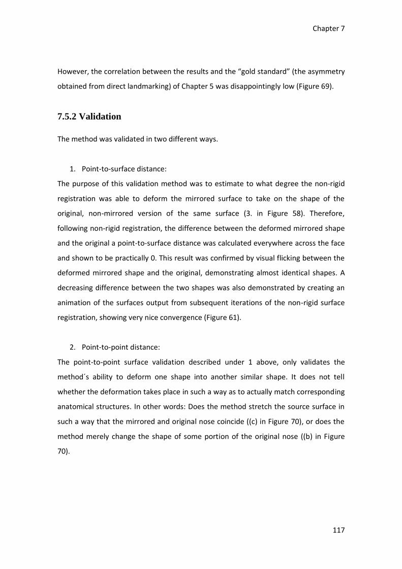
Chapter 7
117
However, the correlation between the results and the “gold standard” (the asymmetry
obtained from direct landmarking) of Chapter 5 was disappointingly low (Figure 69).
7.5.2 Validation
The method was validated in two different ways.
1. Point-to-surface distance:
The purpose of this validation method was to estimate to what degree the non-rigid
registration was able to deform the mirrored surface to take on the shape of the
original, non-mirrored version of the same surface (3. in Figure 58). Therefore,
following non-rigid registration, the difference between the deformed mirrored shape
and the original a point-to-surface distance was calculated everywhere across the face
and shown to be practically 0. This result was confirmed by visual flicking between the
deformed mirrored shape and the original, demonstrating almost identical shapes. A
decreasing difference between the two shapes was also demonstrated by creating an
animation of the surfaces output from subsequent iterations of the non-rigid surface
registration, showing very nice convergence (Figure 61).
2. Point-to-point distance:
The point-to-point surface validation described under 1 above, only validates the
method´s ability to deform one shape into another similar shape. It does not tell
whether the deformation takes place in such a way as to actually match corresponding
anatomical structures. In other words: Does the method stretch the source surface in
such a way that the mirrored and original nose coincide ((c) in Figure 70), or does the
method merely change the shape of some portion of the original nose ((b) in Figure
70).
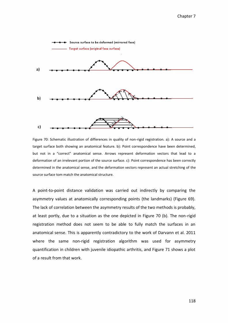
Chapter 7
118
Figure 70: Schematic illustration of differences in quality of non-rigid registration. a): A source and a
target surface both showing an anatomical feature. b): Point correspondence have been determined,
but not in a “correct” anatomical sense. Arrows represent deformation vectors that lead to a
deformation of an irrelevant portion of the source surface. c): Point correspondence has been correctly
determined in the anatomical sense, and the deformation vectors represent an actual stretching of the
source surface tom match the anatomical structure.
A point-to-point distance validation was carried out indirectly by comparing the
asymmetry values at anatomically corresponding points (the landmarks) (Figure 69).
The lack of correlation between the asymmetry results of the two methods is probably,
at least portly, due to a situation as the one depicted in Figure 70 (b). The non-rigid
registration method does not seem to be able to fully match the surfaces in an
anatomical sense. This is apparently contradictory to the work of Darvann et al. 2011
where the same non-rigid registration algorithm was used for asymmetry
quantification in children with juvenile idiopathic arthritis, and Figure 71 shows a plot
of a result from that work.
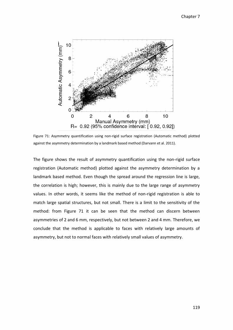
Chapter 7
119
Figure 71: Asymmetry quantification using non-rigid surface registration (Automatic method) plotted
against the asymmetry determination by a landmark based method (Darvann et al. 2011).
The figure shows the result of asymmetry quantification using the non-rigid surface
registration (Automatic method) plotted against the asymmetry determination by a
landmark based method. Even though the spread around the regression line is large,
the correlation is high; however, this is mainly due to the large range of asymmetry
values. In other words, it seems like the method of non-rigid registration is able to
match large spatial structures, but not small. There is a limit to the sensitivity of the
method: from Figure 71 it can be seen that the method can discern between
asymmetries of 2 and 6 mm, respectively, but not between 2 and 4 mm. Therefore, we
conclude that the method is applicable to faces with relatively large amounts of
asymmetry, but not to normal faces with relatively small values of asymmetry.

120
Chapter 8
121
Chapter 8
Facial asymmetry in a larger group
of normal children
8.1 Introduction
The purpose of this work is to quantify the average of facial asymmetry and its
variation in normal children. In this chapter we apply the method developed in Chapter
5 to a large group of normal Caucasian children. The asymmetry quantification is thus
carried out by sparse sets of manually placed landmarks.
Subsequently, a comparison between asymmetry in boys and girls, respectively, is
carried out. Furthermore, it is investigated whether there is a relation between
asymmetry and age.
Last but not least a framework applying principal components analysis (PCA) has been
implemented and applied to this large group of normal children to provide information
about the dominant types of variation in the data.

Chapter 8
122
8.2 Material
The material consisted of 375 3D facial surface scans of normal Caucasian boys and
girls of various ages. 212 of the subjects are boys and 163 are girls. Manually placed
landmarks are located on anatomical structures as shown in Figure 18.
Figure 72 shows a distribution of boys and girls, respectively.
Figure 72: The figure shows histograms of the age of participant children. The figure on top shows the
age of boys and the figure on the bottom show the age of girls. The total number of boys is 212; the
total number of girls is 163.
8.3 Method
The purpose of this chapter is to develop a method to estimate the facial asymmetry in
a sparse set of manually placed landmark locations. The asymmetry was defined as the
geometrical difference between left and right side of the face (Chapter 3). The
asymmetry is estimated using manually placed landmarks on right and left sides of the
face where the asymmetry is the length of the distance between a point and the
0 2 4 6 8 10 12 14 16 180
2
4
6
Age in years
Num
ber
of
subje
cts
Age of boys
0 2 4 6 8 10 12 14 16 180
2
4
6
Age in years
Num
ber
of
subje
cts
Age of girls
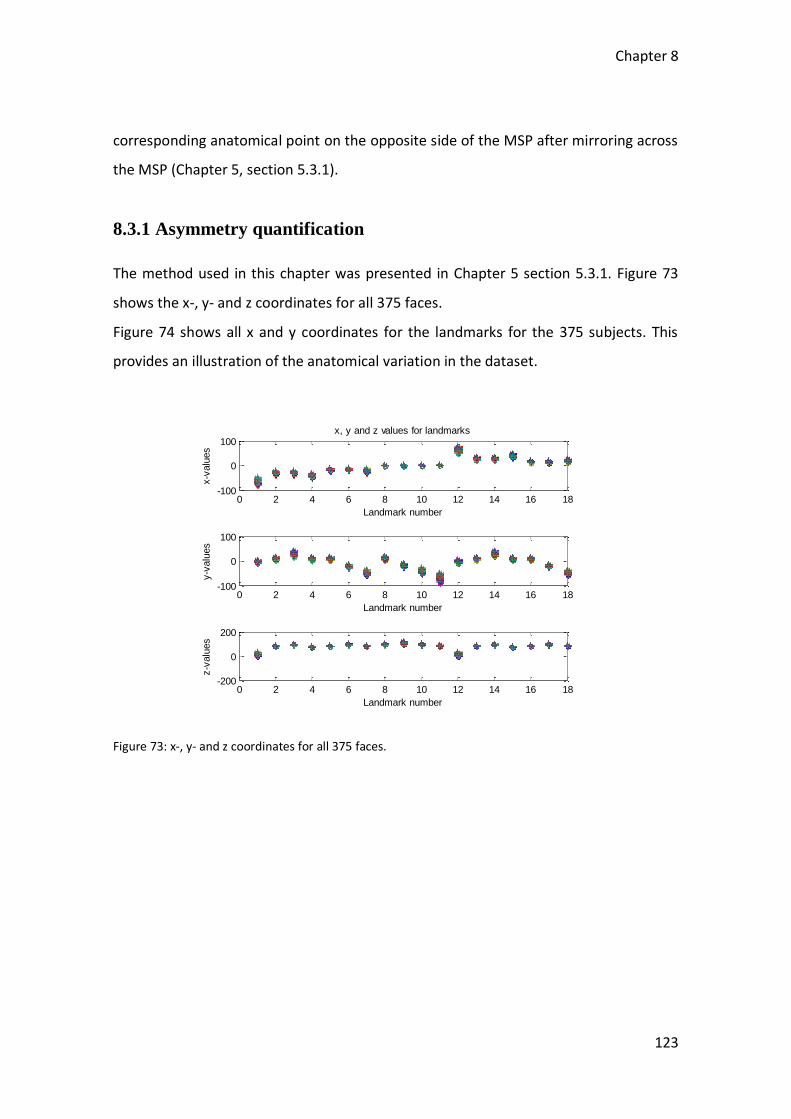
Chapter 8
123
corresponding anatomical point on the opposite side of the MSP after mirroring across
the MSP (Chapter 5, section 5.3.1).
8.3.1 Asymmetry quantification
The method used in this chapter was presented in Chapter 5 section 5.3.1. Figure 73
shows the x-, y- and z coordinates for all 375 faces.
Figure 74 shows all x and y coordinates for the landmarks for the 375 subjects. This
provides an illustration of the anatomical variation in the dataset.
Figure 73: x-, y- and z coordinates for all 375 faces.
0 2 4 6 8 10 12 14 16 18-100
0
100
Landmark number
x-v
alu
es
x, y and z values for landmarks
0 2 4 6 8 10 12 14 16 18-100
0
100
Landmark number
y-v
alu
es
0 2 4 6 8 10 12 14 16 18-200
0
200
Landmark number
z-v
alu
es

Chapter 8
124
Figure 74: The figure shows the x and y landmark coordinates of all faces.
For a description of the method of asymmetry quantification, see section 5.3.1, the
implementation, see section 5.3.2 and the manual landmarking of the face, see section
5.3.3.
After the quantification of the facial asymmetry, the asymmetry is multiplied with a
factor f to correct for size differences since 375 children have different face sizes due
to e.g. age. This means that the correct asymmetry As (size corrected asymmetry) is:
A is the asymmetry where size of shapes is uncorrected and the factor f is:
-80 -60 -40 -20 0 20 40 60 80-100
-50
0
50
x-values
y-v
alu
es
Landmark position for x and y values of every face

Chapter 8
125
CS - centroid size is the square root of sum of squared distances of a set of landmarks
from their centroid (in this case from the landmark of the nose tip).
To obtain the same size for each shape the centroid size for every individual and for
the used template are estimated. Subsequently the factor f is estimated by dividing the
centroid size for the template with the centroid size for the individuals. This factor f is
then multiplied with the asymmetry which induces the correct facial asymmetry for
each face.
Figure 75 shows the x, y and z asymmetry values are shown for each landmark
location.
Figure 75: The figure shows all asymmetry values of x, y and z for every 376 faces.
1 2 3 4 5 6 7 8 9 10 11-10
0
10
Landmark number
x-v
alu
es
x, y and z values of asymmetri of landmarks
1 2 3 4 5 6 7 8 9 10 11-10
0
10
Landmark number
y-v
alu
es
1 2 3 4 5 6 7 8 9 10 11-10
0
10
Landmark number
z-v
alu
es
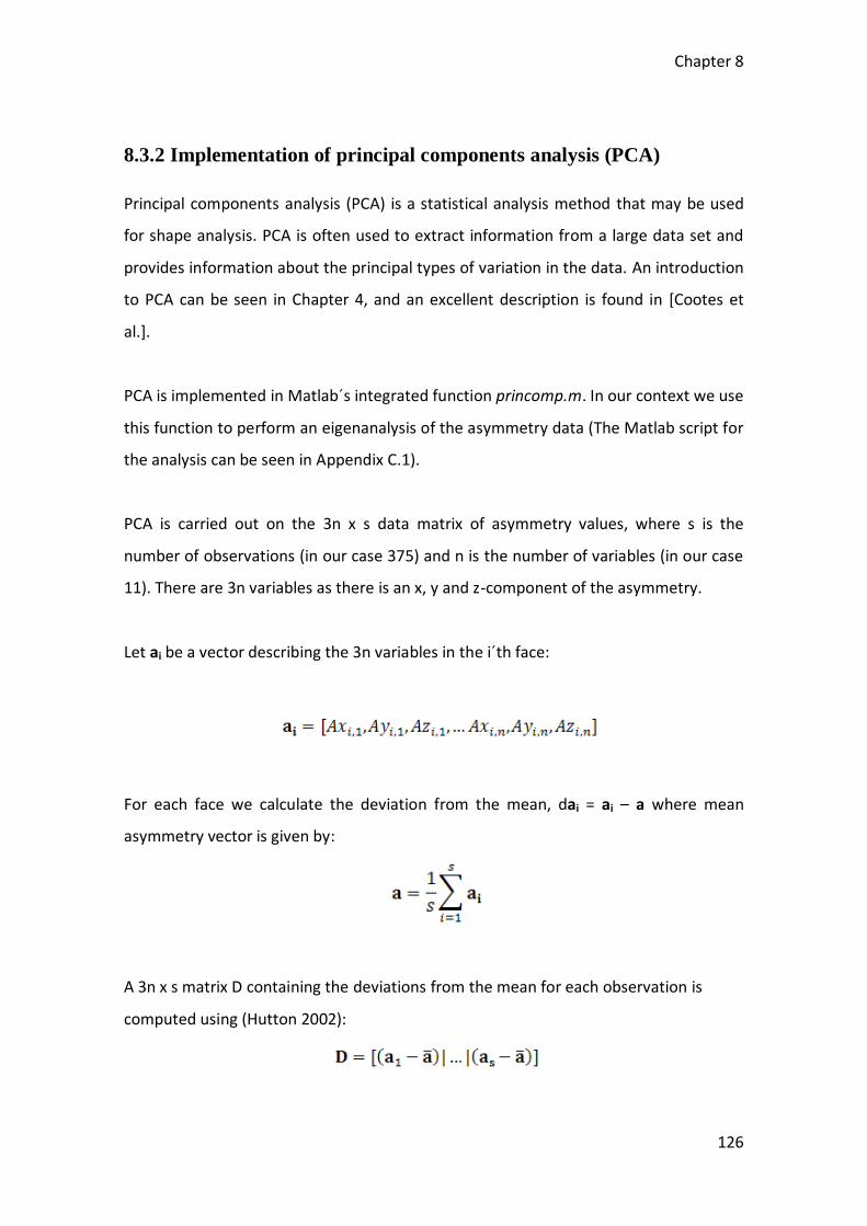
Chapter 8
126
8.3.2 Implementation of principal components analysis (PCA)
Principal components analysis (PCA) is a statistical analysis method that may be used
for shape analysis. PCA is often used to extract information from a large data set and
provides information about the principal types of variation in the data. An introduction
to PCA can be seen in Chapter 4, and an excellent description is found in [Cootes et
al.].
PCA is implemented in Matlab´s integrated function princomp.m. In our context we use
this function to perform an eigenanalysis of the asymmetry data (The Matlab script for
the analysis can be seen in Appendix C.1).
PCA is carried out on the 3n x s data matrix of asymmetry values, where s is the
number of observations (in our case 375) and n is the number of variables (in our case
11). There are 3n variables as there is an x, y and z-component of the asymmetry.
Let ai be a vector describing the 3n variables in the i´th face:
For each face we calculate the deviation from the mean, dai = ai – a where mean
asymmetry vector is given by:
A 3n x s matrix D containing the deviations from the mean for each observation is
computed using (Hutton 2002):
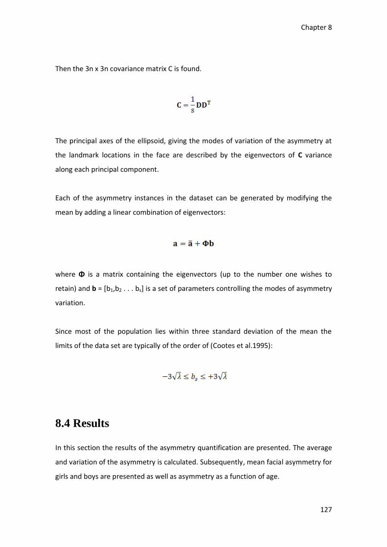
Chapter 8
127
Then the 3n x 3n covariance matrix C is found.
The principal axes of the ellipsoid, giving the modes of variation of the asymmetry at
the landmark locations in the face are described by the eigenvectors of C variance
along each principal component.
Each of the asymmetry instances in the dataset can be generated by modifying the
mean by adding a linear combination of eigenvectors:
where Φ is a matrix containing the eigenvectors (up to the number one wishes to
retain) and b = [b1,b2 . . . bs] is a set of parameters controlling the modes of asymmetry
variation.
Since most of the population lies within three standard deviation of the mean the
limits of the data set are typically of the order of (Cootes et al.1995):
8.4 Results
In this section the results of the asymmetry quantification are presented. The average
and variation of the asymmetry is calculated. Subsequently, mean facial asymmetry for
girls and boys are presented as well as asymmetry as a function of age.

Chapter 8
128
8.4.1 Asymmetry quantification
Figure 76 shows boxplots of facial asymmetry in each face. As seen the mean facial
asymmetry for the faces is approximately 2 mm.
Figure 76: Boxplots of amount of asymmetry (in mm) in each of the 375 faces.
Figure 77 shows the asymmetry for each landmark. The asymmetry is shown by
boxplots, which contain asymmetry values for every face in a landmark location. In
Figure 78 the amount of asymmetry is shown again. The amount of asymmetry is now
plotted as a plot where each asymmetry value is shown by points in different colors.

Chapter 8
129
Figure 77: Boxplots indicating the distribution of asymmetry for all 375 faces for each of the 11 landmark
locations.
Figure 78: Asymmetry values of each face in different landmark point. Different colors are used to
illustrate the asymmetry for landmark points for different faces. This makes it easier to see the different
landmark points.
Figure 79 and 80 shows mean-, standard deviation-, maximum- and minimum
asymmetry values of each landmark location and for each face, respectively.
0
1
2
3
4
5
6
7
8
9
1 2 3 4 5 6 7 8 9 10 11Landmark number
Asym
metr
y (
mm
)
Asymmetry of each face in different points
1 2 3 4 5 6 7 8 9 10 110
1
2
3
4
5
6
7
8
9
Landmark number
Asym
metr
y (
mm
)
Asymmetri values of each point in all faces
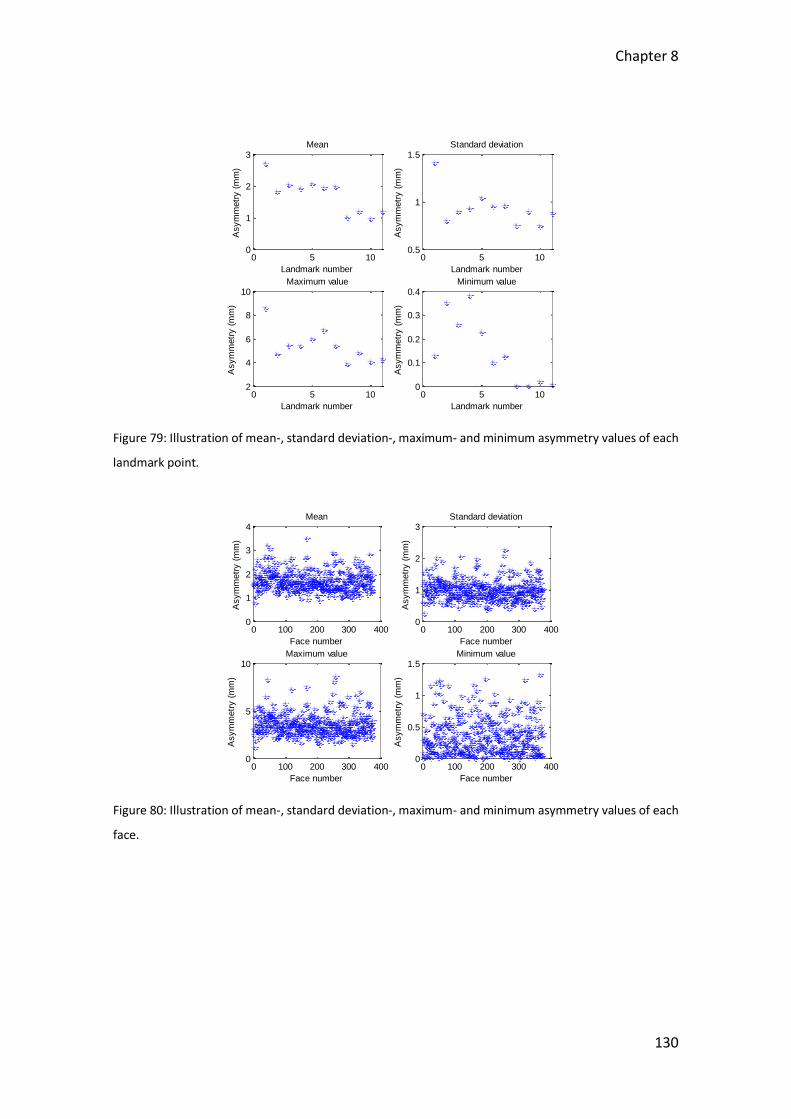
Chapter 8
130
Figure 79: Illustration of mean-, standard deviation-, maximum- and minimum asymmetry values of each
landmark point.
Figure 80: Illustration of mean-, standard deviation-, maximum- and minimum asymmetry values of each
face.
0 5 100
1
2
3
Landmark number
Asym
metr
y (
mm
)
Mean
0 5 100.5
1
1.5
Landmark number
Asym
metr
y (
mm
)
Standard deviation
0 5 102
4
6
8
10
Landmark number
Asym
metr
y (
mm
)
Maximum value
0 5 100
0.1
0.2
0.3
0.4
Landmark numberA
sym
metr
y (
mm
)
Minimum value
0 100 200 300 4000
1
2
3
4
Face number
Asym
metr
y (
mm
)
Mean
0 100 200 300 4000
1
2
3
Face number
Asym
metr
y (
mm
)
Standard deviation
0 100 200 300 4000
5
10
Face number
Asym
metr
y (
mm
)
Maximum value
0 100 200 300 4000
0.5
1
1.5
Face number
Asym
metr
y (
mm
)
Minimum value
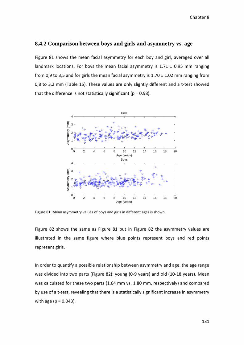
Chapter 8
131
8.4.2 Comparison between boys and girls and asymmetry vs. age
Figure 81 shows the mean facial asymmetry for each boy and girl, averaged over all
landmark locations. For boys the mean facial asymmetry is 1.71 ± 0.95 mm ranging
from 0,9 to 3,5 and for girls the mean facial asymmetry is 1.70 ± 1.02 mm ranging from
0,8 to 3,2 mm (Table 15). These values are only slightly different and a t-test showed
that the difference is not statistically significant (p = 0.98).
Figure 81: Mean asymmetry values of boys and girls in different ages is shown.
Figure 82 shows the same as Figure 81 but in Figure 82 the asymmetry values are
illustrated in the same figure where blue points represent boys and red points
represent girls.
In order to quantify a possible relationship between asymmetry and age, the age range
was divided into two parts (Figure 82): young (0-9 years) and old (10-18 years). Mean
was calculated for these two parts (1.64 mm vs. 1.80 mm, respectively) and compared
by use of a t-test, revealing that there is a statistically significant increase in asymmetry
with age (p = 0.043).
0 2 4 6 8 10 12 14 16 18 200
1
2
3
4
Age (years)
Asym
metr
y (
mm
)
Girls
0 2 4 6 8 10 12 14 16 18 200
1
2
3
4
Age (years)
Asym
metr
y (
mm
)
Boys

Chapter 8
132
Figure 82: Mean asymmetry values of boys (blue) and girls (red) as a function of age. Green horizontal
lines represent the mean values in the two age ranges 0-9 years and 10-18 years, respectively. The green
vertical line divide the two age ranges. The black line illustrates that the asymmetry increase with age.
Table 15: The mean asymmetry, standard deviation (SD) and p-values for boys and girls
Asymmetry Mean boys Mean girls SD (boys) SD (girls) P-value (t-test)
Ear 2.59 2.85 1.34 1.49 0.078
Eye center 1.77 1.87 0.73 0.88 0.2578
Eye brow 1.99 2.08 0.87 0.93 0.3812
Eye outer corner 1.85 2.00 0.91 0.97 0.1143
Eye inner corner 2.09 2.02 1.03 1.05 0.4957
Nose corner 1.99 1.86 1.01 0.88 0.1727
Mouth corner 2.01 1.93 0.98 0.94 0.4825
Nasion 1.06 0.93 0.79 0.69 0.0989
Nose tip 1.17 1.17 0.92 0.87 0.982
Upper lip 0.97 0.96 0.78 0.72 0.837
Chin 1.34 0.99 0.94 0.75 0.0001
Face 1.71 1.70 0.95 1.02 0.979
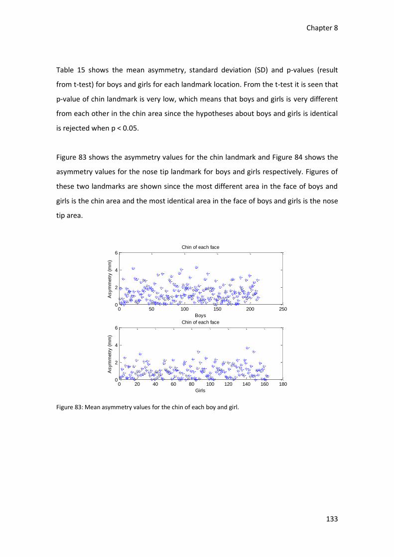
Chapter 8
133
Table 15 shows the mean asymmetry, standard deviation (SD) and p-values (result
from t-test) for boys and girls for each landmark location. From the t-test it is seen that
p-value of chin landmark is very low, which means that boys and girls is very different
from each other in the chin area since the hypotheses about boys and girls is identical
is rejected when p < 0.05.
Figure 83 shows the asymmetry values for the chin landmark and Figure 84 shows the
asymmetry values for the nose tip landmark for boys and girls respectively. Figures of
these two landmarks are shown since the most different area in the face of boys and
girls is the chin area and the most identical area in the face of boys and girls is the nose
tip area.
Figure 83: Mean asymmetry values for the chin of each boy and girl.
0 50 100 150 200 2500
2
4
6
Boys
Asym
metr
y (
mm
)
Chin of each face
0 20 40 60 80 100 120 140 160 1800
2
4
6
Girls
Asym
metr
y (
mm
)
Chin of each face
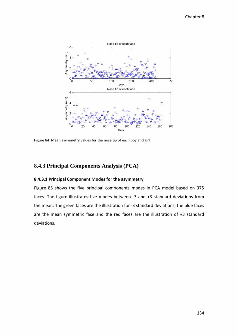
Chapter 8
134
Figure 84: Mean asymmetry values for the nose tip of each boy and girl.
8.4.3 Principal Components Analysis (PCA)
8.4.3.1 Principal Component Modes for the asymmetry
Figure 85 shows the five principal components modes in PCA model based on 375
faces. The figure illustrates five modes between -3 and +3 standard deviations from
the mean. The green faces are the illustration for -3 standard deviations, the blue faces
are the mean symmetric face and the red faces are the illustration of +3 standard
deviations.
0 50 100 150 200 2500
2
4
6
Boys
Asym
metr
y (
mm
)
Nose tip of each face
0 20 40 60 80 100 120 140 160 1800
2
4
6
Girls
Asym
metr
y (
mm
)
Nose tip of each face
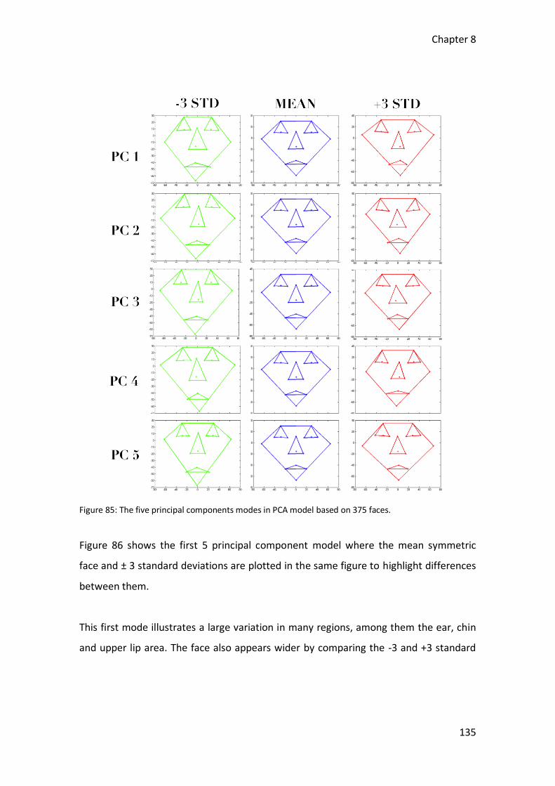
Chapter 8
135
Figure 85: The five principal components modes in PCA model based on 375 faces.
Figure 86 shows the first 5 principal component model where the mean symmetric
face and ± 3 standard deviations are plotted in the same figure to highlight differences
between them.
This first mode illustrates a large variation in many regions, among them the ear, chin
and upper lip area. The face also appears wider by comparing the -3 and +3 standard

Chapter 8
136
deviation. Second, fourth and fifth modes illustrate also a large variation in many
regions while third mode illustrates a large variation in the nasion region.
(a)
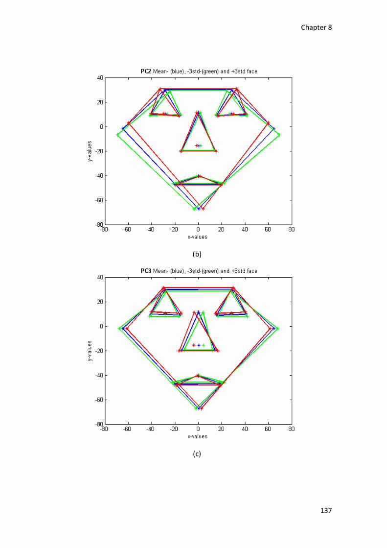
Chapter 8
137
(b)
(c)
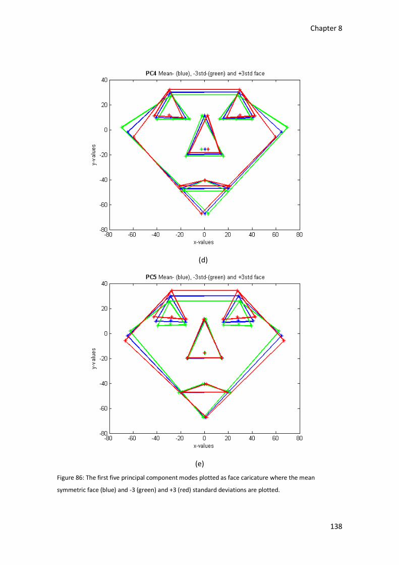
Chapter 8
138
(d)
(e)
Figure 86: The first five principal component modes plotted as face caricature where the mean
symmetric face (blue) and -3 (green) and +3 (red) standard deviations are plotted.
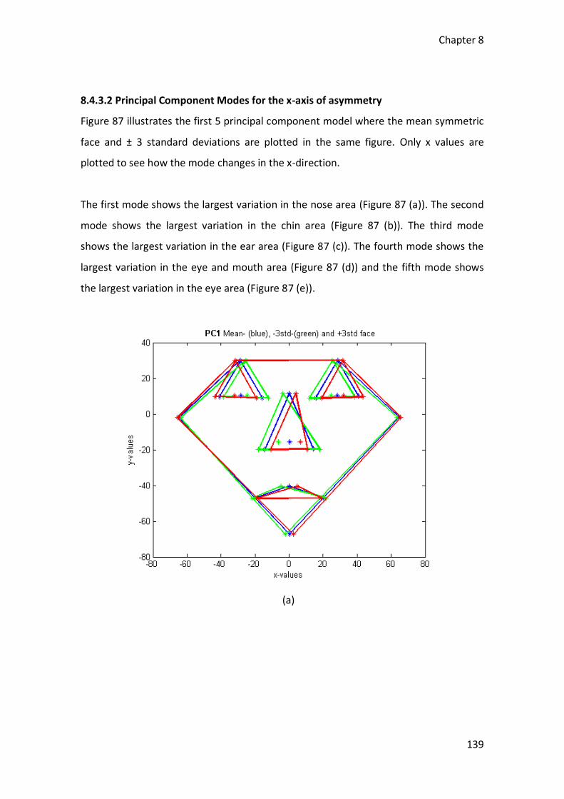
Chapter 8
139
8.4.3.2 Principal Component Modes for the x-axis of asymmetry
Figure 87 illustrates the first 5 principal component model where the mean symmetric
face and ± 3 standard deviations are plotted in the same figure. Only x values are
plotted to see how the mode changes in the x-direction.
The first mode shows the largest variation in the nose area (Figure 87 (a)). The second
mode shows the largest variation in the chin area (Figure 87 (b)). The third mode
shows the largest variation in the ear area (Figure 87 (c)). The fourth mode shows the
largest variation in the eye and mouth area (Figure 87 (d)) and the fifth mode shows
the largest variation in the eye area (Figure 87 (e)).
(a)
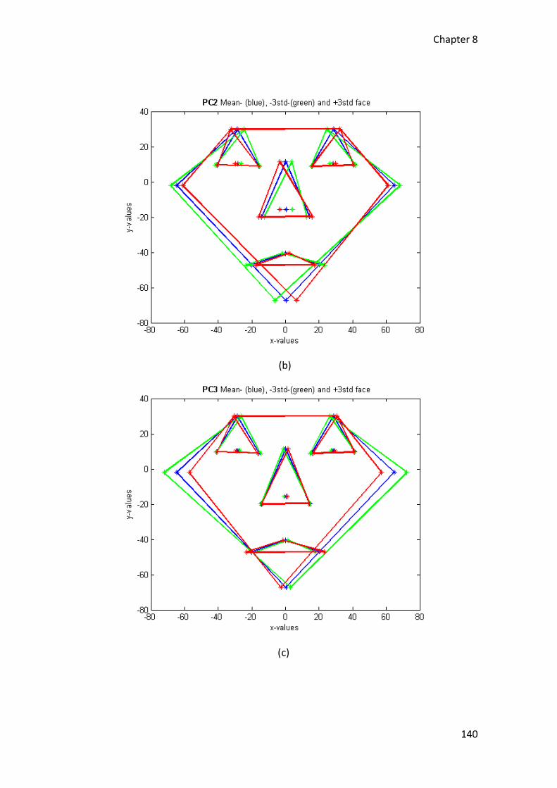
Chapter 8
140
(b)
(c)
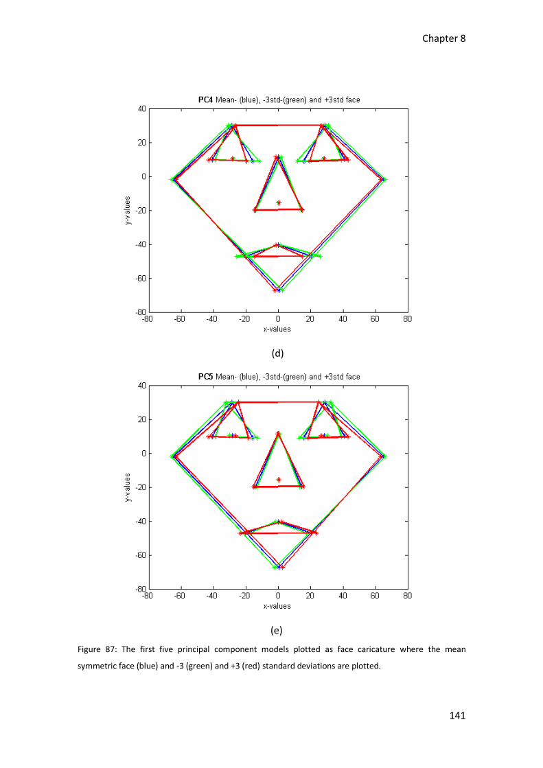
Chapter 8
141
(d)
(e)
Figure 87: The first five principal component models plotted as face caricature where the mean
symmetric face (blue) and -3 (green) and +3 (red) standard deviations are plotted.

Chapter 8
142
8.4.3.3 Principal Component Modes for the y-axis of asymmetry
Figure 88 shows the first 5 principal component modes for y-direction of asymmetry.
This first, second, third, fourth and fifth modes illustrate a large variation in the ear,
eyebrow, eye and eyebrow, mouth and eye area, respectively.
(a)
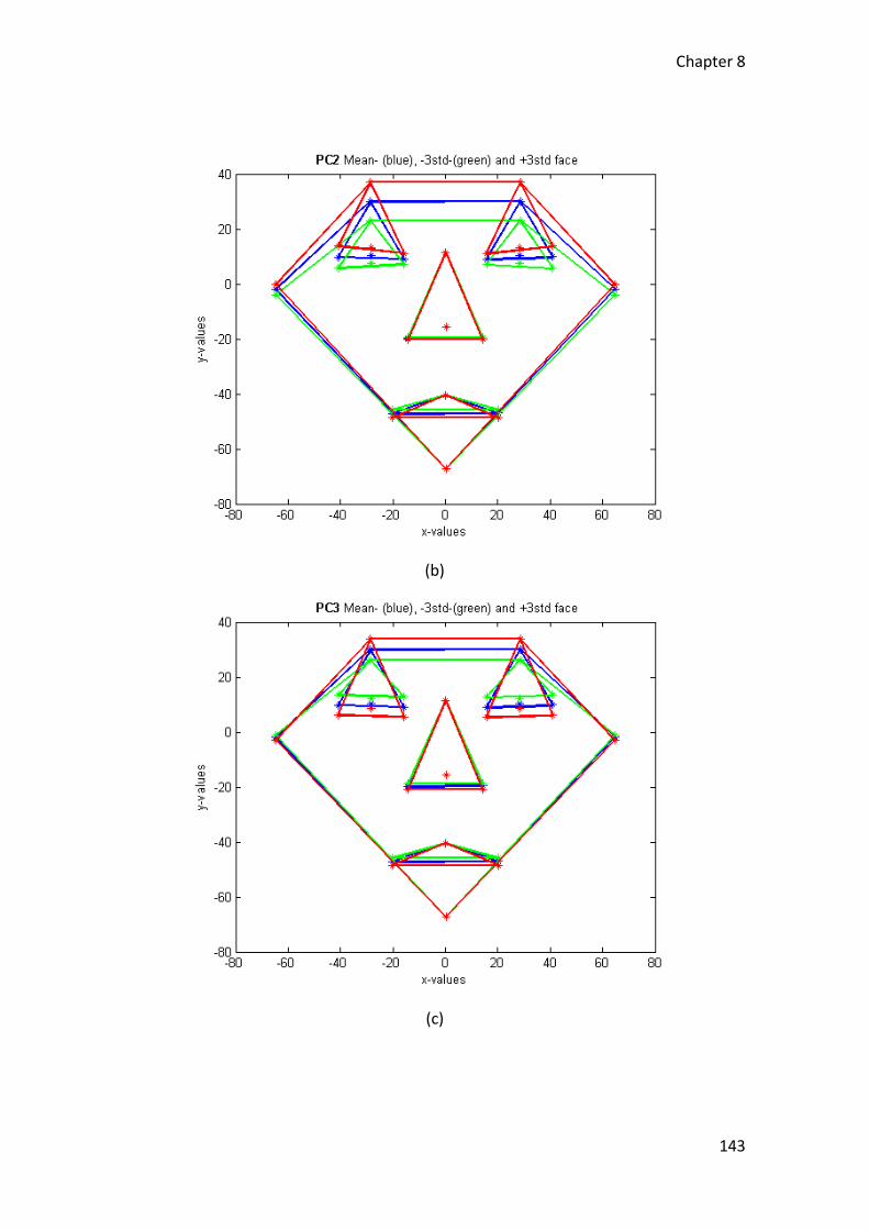
Chapter 8
143
(b)
(c)

Chapter 8
144
(d)
(e)
Figure 88: The first five principal component models plotted as face caricature where the mean
symmetric face (blue) and -3 (green) and +3 (red) standard deviations are plotted.
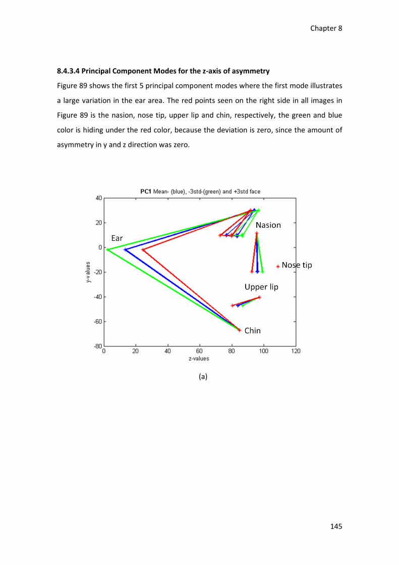
Chapter 8
145
8.4.3.4 Principal Component Modes for the z-axis of asymmetry
Figure 89 shows the first 5 principal component modes where the first mode illustrates
a large variation in the ear area. The red points seen on the right side in all images in
Figure 89 is the nasion, nose tip, upper lip and chin, respectively, the green and blue
color is hiding under the red color, because the deviation is zero, since the amount of
asymmetry in y and z direction was zero.
(a)

Chapter 8
146
(b)
(c)

Chapter 8
147
(d)
(e)
Figure 89: The first five principal component models plotted as face caricature where the mean
symmetric face (blue) and -3 (green) and +3 (red) standard deviations are plotted.

Chapter 8
148
8.4.3.5 Principal Component Score plots
Figure 90 shows the score plots (values of the principal component variables) for the
different modes up to mode five. The red points represent each of the faces included
in the PCA. The location of each face is depending on the amount of asymmetry, where
the faces with the lowest amount of asymmetry are in the middle of each score plot,
while the faces with the highest amount of asymmetry are located in the outer region
of the plot. The types of variation represented along the axes in each score plot may
be found by inspecting the corresponding mode plots in Figures 85 and 86.
Figure 90: Score plots for the first 5 principal components.
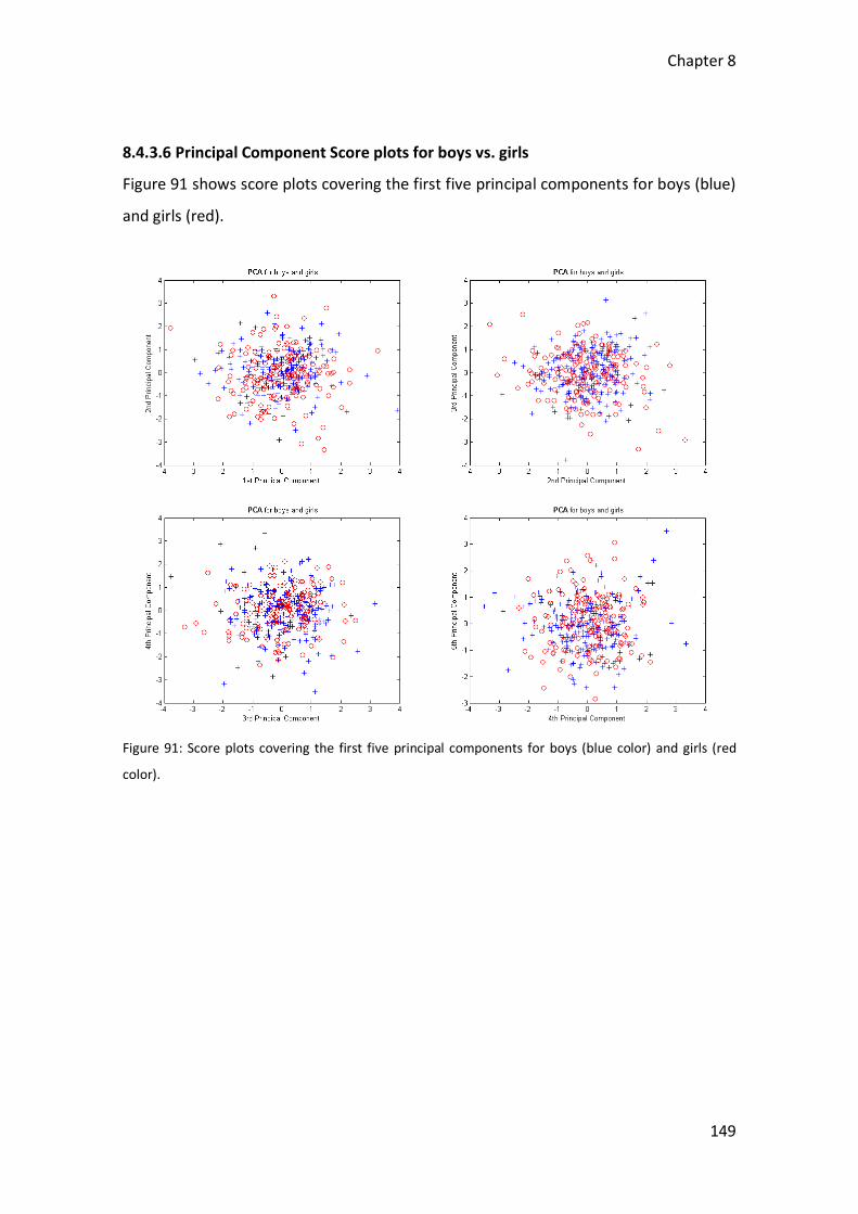
Chapter 8
149
8.4.3.6 Principal Component Score plots for boys vs. girls
Figure 91 shows score plots covering the first five principal components for boys (blue)
and girls (red).
Figure 91: Score plots covering the first five principal components for boys (blue color) and girls (red
color).

Chapter 8
150
8.4.3.7 Total variance percentage
Figure 92: Percent variability explained by each principal component for the magnitude of asymmetry.
Figure 92 shows the amount of variance that each of the modes contributes to total
variance.
8.5 Discussion
8.5.1 Asymmetry for the faces and landmark locations
In this chapter the facial asymmetry was quantified in 375 normal children. Given this
large number of individuals included in the sample, an accurate estimate of the mean
asymmetry, as well as its variation, in the two populations can be found. Mean and
variation was estimated in each landmark location (representing different facial
regions) as well as for the whole face (average of all landmark locations).
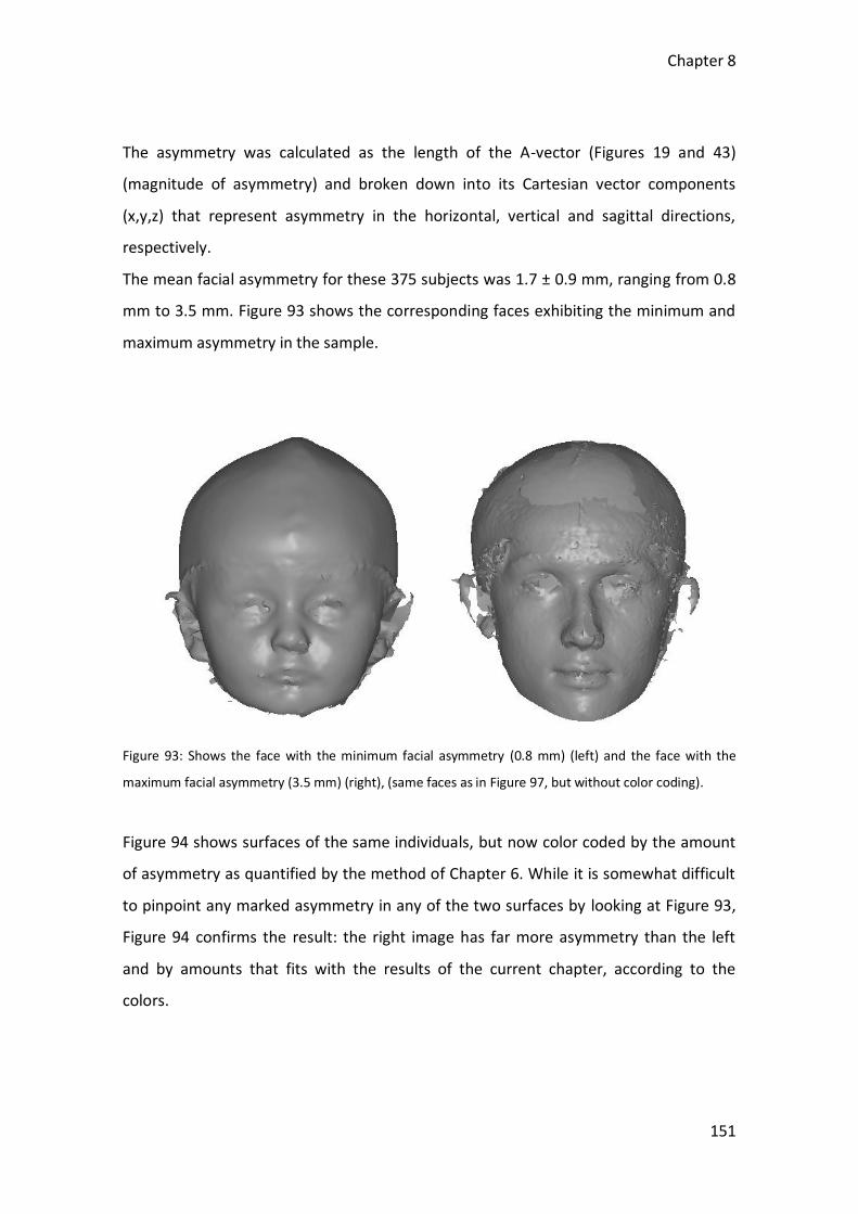
Chapter 8
151
The asymmetry was calculated as the length of the A-vector (Figures 19 and 43)
(magnitude of asymmetry) and broken down into its Cartesian vector components
(x,y,z) that represent asymmetry in the horizontal, vertical and sagittal directions,
respectively.
The mean facial asymmetry for these 375 subjects was 1.7 ± 0.9 mm, ranging from 0.8
mm to 3.5 mm. Figure 93 shows the corresponding faces exhibiting the minimum and
maximum asymmetry in the sample.
Figure 93: Shows the face with the minimum facial asymmetry (0.8 mm) (left) and the face with the
maximum facial asymmetry (3.5 mm) (right), (same faces as in Figure 97, but without color coding).
Figure 94 shows surfaces of the same individuals, but now color coded by the amount
of asymmetry as quantified by the method of Chapter 6. While it is somewhat difficult
to pinpoint any marked asymmetry in any of the two surfaces by looking at Figure 93,
Figure 94 confirms the result: the right image has far more asymmetry than the left
and by amounts that fits with the results of the current chapter, according to the
colors.

Chapter 8
152
Figure 94: Shows the face with the minimum facial asymmetry (left) and the face with the maximum
facial asymmetry (right), as quantified by the method of Chapter 6.
It is obvious that the nose area contains more asymmetry in both faces. This can
depend on the manual landmark setting; because it was concluded in Chapter 6, that
manual landmark setting have influence on the result of facial asymmetry. Here, it was
also concluded that a better result was achieved when some extra landmarks were set
in specific locations in the nose area. Therefore the amount of mean facial asymmetry
could be a little lower if some extra landmarks were set in the nose area.
Also, it could possibly be a good idea to look away from the variation for the landmark
of the ear since manual landmark setting in this location can be very difficult.
According to these facial asymmetry results, it would be unlikely that a face with a
larger amount of asymmetry than the maximum value (3.5 mm) would be part of the
“normal” population. Or, more formally, one could choose a limit of 2 standard
deviations (1.7 mm + 2 x 0.9 mm = 3.5 mm) to begin to suspect abnormality in terms of
asymmetry. Having established this kind of reference values could be used as a
comparison to values obtained in a patient, both for diagnostic purposes and for
treatment progression monitoring and evaluation.

Chapter 8
153
8.5.3 Asymmetry relation for boys and girls and asymmetry vs. age
We hypothesized that there might be a difference in asymmetry between boys and
girls, and that boys would be most asymmetric of the two. Reasons for this could be
genetic: the importance of attractiveness in terms of asymmetry when choosing a
mate could for some reason be stronger in men. Since the face of males is larger
(especially from puberty and onwards) and has more marked features (especially the
lower jaw that grows much faster in boys in puberty) one might argue that there is
more opportunity for small growth “accidents” (leading to more asymmetry) in males
than in females, and especially in the lower part of the face.
Reasons could also be environmental: boys could have a tendency to be involved in
more physical activity (fighting, high risk sports) than girls. Again this might affect the
most prominent features of the face, like the nose and chin.
Indeed, when looking at the results, boys have slightly larger asymmetry (for the whole
face) than girls, although not statistically significant (Table 15). Perhaps the difference
would become statistically significant if the number of individuals included in the study
had been even larger.
Also, when comparing boys and girls in term of asymmetry in the 11 different face
regions (Table 15), there were no statistically significant differences, expect for the
chin region.
However, although not statistically significantly different except for the chin, boys had
larger asymmetry than girls in almost all regions in the lower face (nose, lip, mouth and
chin). This would seem to fit in with the hypothesis of the male jaw becoming more
asymmetric. This is clearly the case for the chin landmark where there was a highly
statistically significant higher asymmetry in boys than in girls. This landmark is only one

Chapter 8
154
located in such a way as to represent the lower jaw; a bone that grows very different
in the two genders.
As a corollary of the first hypothesis, one would hypothesize that asymmetry would
increase with age (more time for asymmetry to develop). Such a statistically significant
increase of asymmetry was found (Figure 82 (p = 0.043)), supporting this last
hypothesis.
8.5.4 PCA
The score plots (Figure 90) show a beautiful circularly shaped multi-dimensional
normal distribution-like point cloud, indicating that the data are well suited for PCA
[Cootes et al.].
In general, plots (Figure 85-89) show a lot of co-variation between various regions, and
none of the modes represent a variation of only one or a couple of regions. This is
different from typical results of studies of asymmetry in groups of individuals with
particular craniofacial anomalies.
An example of the latter is a study of deformational plagiocephaly by Lanche et al.
where the two first modes are found to almost solely represent variation at two
localized regions of the head, respectively.
However, in our study of normal individuals, we would not expect any particular region
to vary more than others. The small “accidents” that occur in the course of
development of the face take place in totally different locations in different
individuals, shaping each face in a unique way. This is manifested in the mode plots
that appear very spatially un-specific. It is also reflected in the scree-plot (Figure 92)
where even the first mode shows low variance (16 %), and a large number of principal
components are needed in order to explain a significant proportion of the total
variance. Again this result (from the analysis of manual population) is different from a

Chapter 8
155
result of a study of disease: Figure 95 shows the scree-plot from the study of
plagiocephaly by Lanche et al., where the first mode explains as much as 60 % of the
total variation.
Figure 95: Scree plot of the study of Lanche et al. where the two first modes are represent variation at
two regions of the head.
In order to discuss the connection between score plots, mode plots and the
asymmetry in a particular region, we pick a mode plot that is mainly dominated by
variation in one region: PC3 for the PCA model of asymmetry in the x-direction (Figure
87 (c)) show a dominant variation in the ear. A corresponding score plot, showing PC3
vs. PC4 is shown in Figure 96.
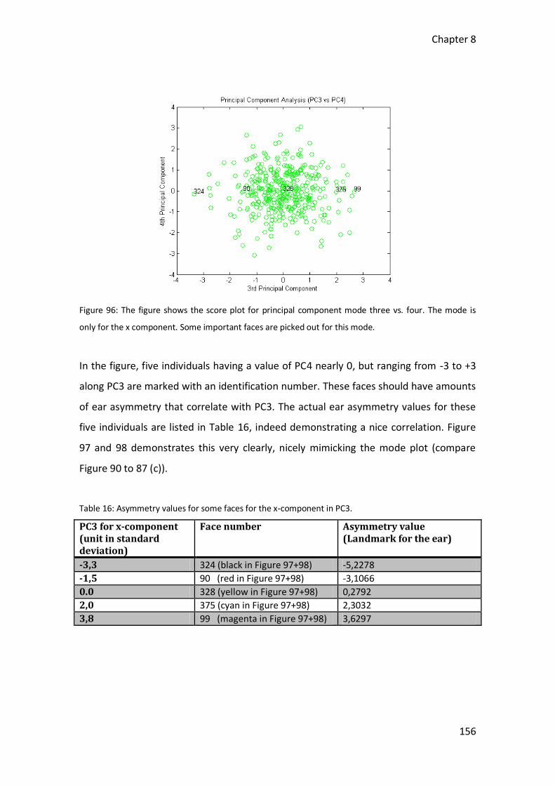
Chapter 8
156
Figure 96: The figure shows the score plot for principal component mode three vs. four. The mode is
only for the x component. Some important faces are picked out for this mode.
In the figure, five individuals having a value of PC4 nearly 0, but ranging from -3 to +3
along PC3 are marked with an identification number. These faces should have amounts
of ear asymmetry that correlate with PC3. The actual ear asymmetry values for these
five individuals are listed in Table 16, indeed demonstrating a nice correlation. Figure
97 and 98 demonstrates this very clearly, nicely mimicking the mode plot (compare
Figure 90 to 87 (c)).
Table 16: Asymmetry values for some faces for the x-component in PC3.
PC3 for x-component (unit in standard deviation)
Face number Asymmetry value (Landmark for the ear)
-3,3 324 (black in Figure 97+98) -5,2278
-1,5 90 (red in Figure 97+98) -3,1066
0.0 328 (yellow in Figure 97+98) 0,2792
2,0 375 (cyan in Figure 97+98) 2,3032
3,8 99 (magenta in Figure 97+98) 3,6297
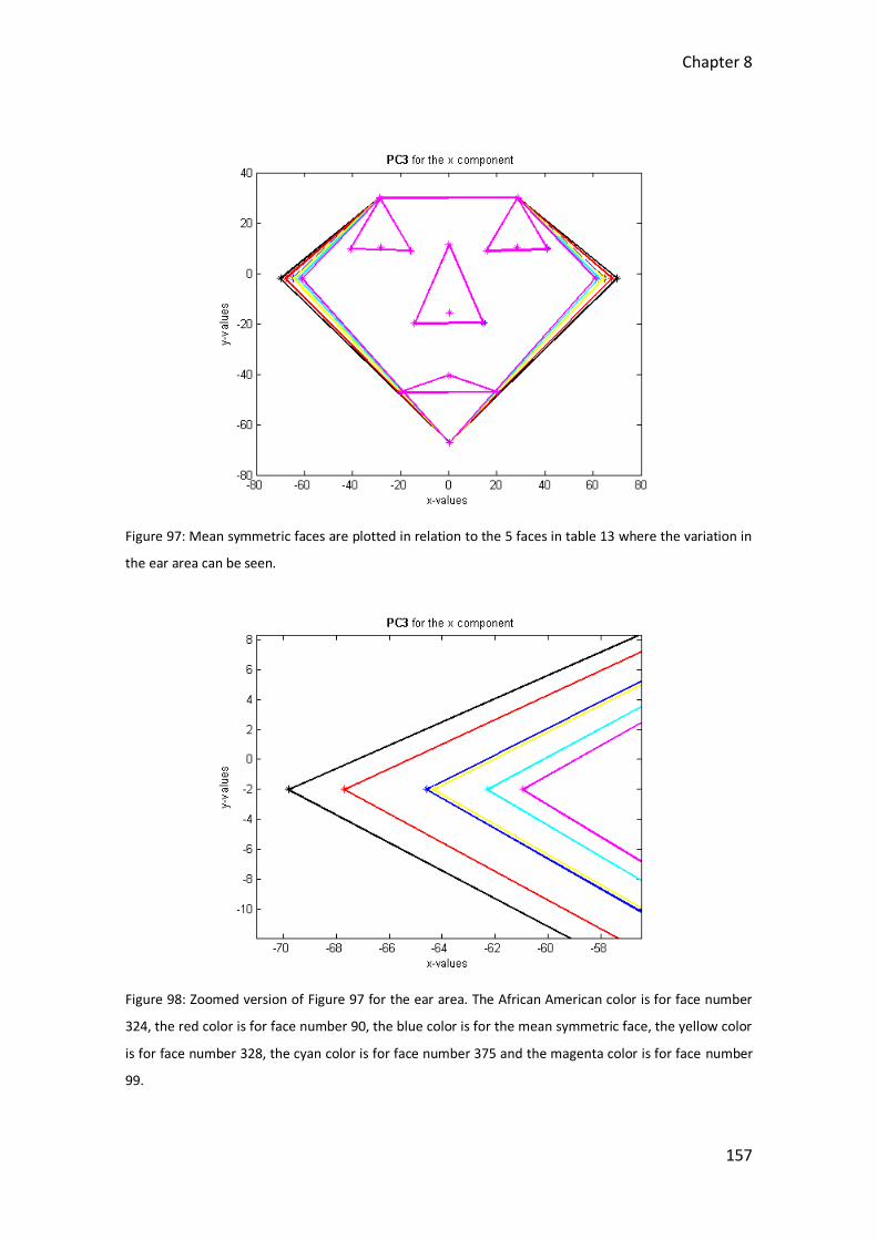
Chapter 8
157
Figure 97: Mean symmetric faces are plotted in relation to the 5 faces in table 13 where the variation in
the ear area can be seen.
Figure 98: Zoomed version of Figure 97 for the ear area. The African American color is for face number
324, the red color is for face number 90, the blue color is for the mean symmetric face, the yellow color
is for face number 328, the cyan color is for face number 375 and the magenta color is for face number
99.

Chapter 8
158
8.6 Conclusion
In this chapter, facial asymmetry was estimated in 375 normal subjects, representing
the largest data base of normative data of this kind known to us.
The asymmetry and its variation for the face as whole, as well as for sub-regions of the
face were calculated and tabulated (Table 15). This result may be used as a normative
reference in connection with patient treatment (diagnostic, treatment planning,
monitoring of treatment progression, treatment evaluation) and in studies of the
biology of normality and disease.
Some of the major findings:
Mean facial asymmetry in the normal population is 1.7 ± 0.9 mm.
Boys have a tendency to be more asymmetric than girls, but this is only
statistically significant in the chin region.
Asymmetry increases with age.
Asymmetry and its variation is not confined to, or dominated by, any particular
part of the face.

Chapter 9
159
Chapter 9
Principal Components Analysis for
quantification of differences in
asymmetry between different types
of craniofacial anomalies and
normal population
9.1 Introduction
The purpose of this chapter is to investigate whether principal components analysis
(PCA) of asymmetry (Section 4.9 and 8.3.2) can distinguish between normal children
and different types of craniofacial anomalies.
Furthermore, to what extent PCA is able to recover interpretable modes of variation
that can describe types of asymmetry that separates a particular craniofacial anomaly
from normal population.
9.2 Material
In this chapter, facial asymmetry is estimated in 451 3D facial surface scans of children
of various ages. 375 of the facial surfaces scans originate from normal children (no
history of craniofacial disease or trauma), 26, 22 and 28 of the facial surface scans

Chapter 9
160
originate from children with diagnosis of cleft-left and palate (CLP), children with
diagnosis of juvenile idiopathic arthritis (JIA) and children with diagnosis of unilateral
coronal suture synostosis (UCS), respectively, (see section 1.2 to further information
on each type of anomaly).
As in Chapter 8, the PCA is performed on asymmetry values obtained at 11 manually
placed landmarks representing different facial regions.
9.3 Method
The method used in this chapter is identical to the method of Chapter 8 (Section 8.3).
Also a description of the method for the asymmetry quantification and the
implementation of the PCA can be found in Chapter 8 (sees section 8.3.1 and section
8.3.2).
9.4 Results
9.4.1 Asymmetry quantification
The mean asymmetry (length of asymmetry vector) for different types of craniofacial
anomalies can be seen by means of boxplots (containing all 11 landmark locations)
(Figure 99).
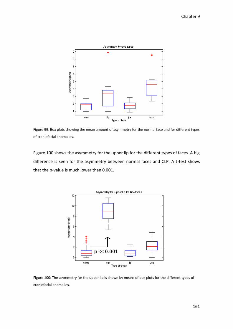
Chapter 9
161
Figure 99: Box plots showing the mean amount of asymmetry for the normal face and for different types
of craniofacial anomalies.
Figure 100 shows the asymmetry for the upper lip for the different types of faces. A big
difference is seen for the asymmetry between normal faces and CLP. A t-test shows
that the p-value is much lower than 0.001.
Figure 100: The asymmetry for the upper lip is shown by means of box plots for the different types of
craniofacial anomalies.
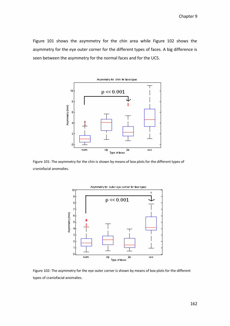
Chapter 9
162
Figure 101 shows the asymmetry for the chin area while Figure 102 shows the
asymmetry for the eye outer corner for the different types of faces. A big difference is
seen between the asymmetry for the normal faces and for the UCS.
Figure 101: The asymmetry for the chin is shown by means of box plots for the different types of
craniofacial anomalies.
Figure 102: The asymmetry for the eye outer corner is shown by means of box plots for the different
types of craniofacial anomalies.
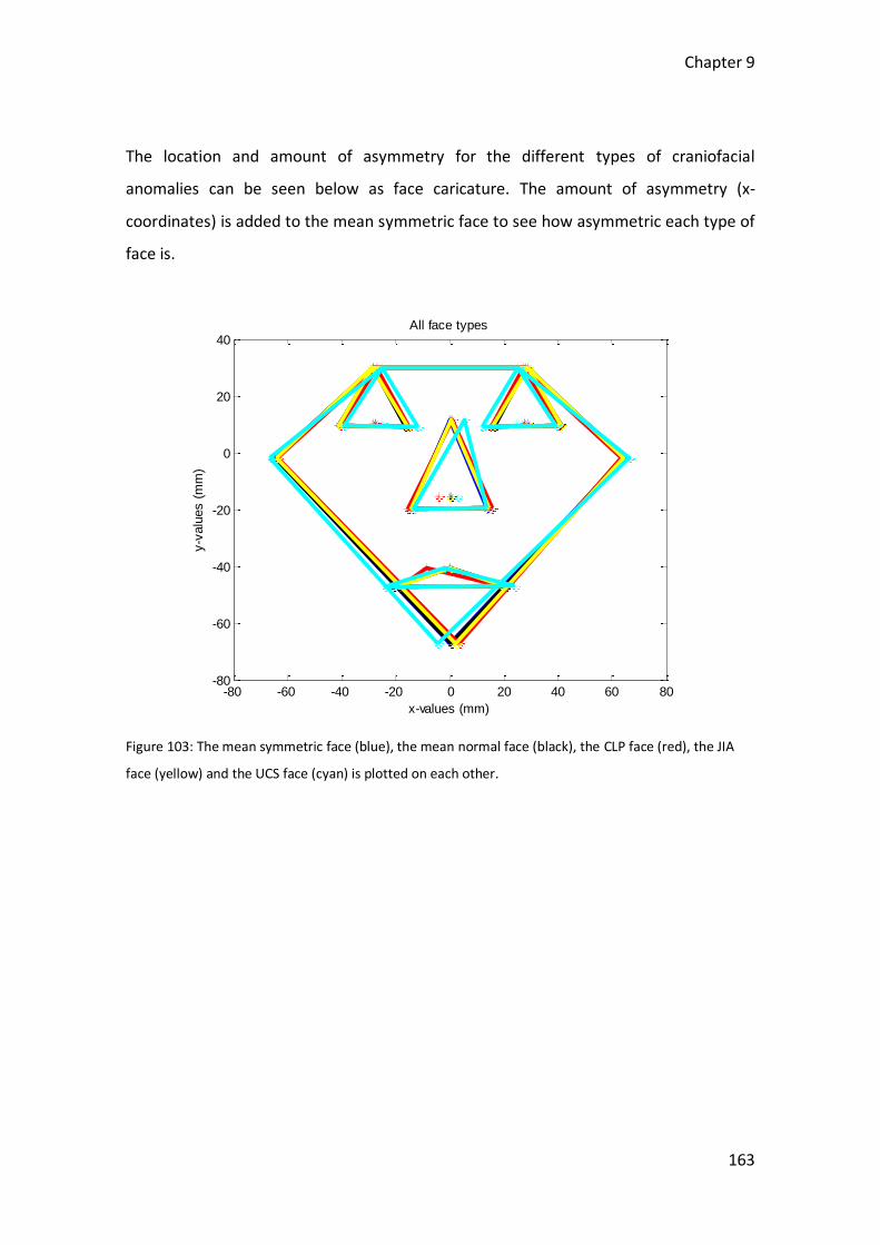
Chapter 9
163
The location and amount of asymmetry for the different types of craniofacial
anomalies can be seen below as face caricature. The amount of asymmetry (x-
coordinates) is added to the mean symmetric face to see how asymmetric each type of
face is.
Figure 103: The mean symmetric face (blue), the mean normal face (black), the CLP face (red), the JIA
face (yellow) and the UCS face (cyan) is plotted on each other.
-80 -60 -40 -20 0 20 40 60 80-80
-60
-40
-20
0
20
40
x-values (mm)
y-v
alu
es (
mm
)
All face types

Chapter 9
164
(a) (b)
(c) (d)
Figure 104: All figures show the mean symmetric face with the mean normal, mean CLP, mean JIA and
mean UCS face is plotted on the mean symmetric face in Figure (a), (b), (c) and (d), respectively. The
amount of asymmetry is added to mean symmetric face to see how asymmetric each type of face is.
Only the x-coordinates are added, therefore the face caricatures are moving only in x-direction.
Figure 104 (a) shows small differences between the mean symmetric face and the
mean normal face. Figure 104 (b) (face with diagnosis of CLP), (c) (face with diagnosis
of JIA) and (d) (face with diagnosis of UCS) show larger differences compared to the
mean symmetric face.
Table 17 shows the mean asymmetry (magnitude) for the different types of
craniofacial anomalies. It is seen that the asymmetry is different in different areas of
the face for different types of craniofacial anomalies and the normal population.
-80 -60 -40 -20 0 20 40 60 80-80
-60
-40
-20
0
20
40
x-values (mm)
y-v
alu
es (
mm
)
Mean face and normal faces
-80 -60 -40 -20 0 20 40 60 80-80
-60
-40
-20
0
20
40
x-values (mm)
y-v
alu
es (
mm
)
Mean face and CLP faces
-80 -60 -40 -20 0 20 40 60 80-80
-60
-40
-20
0
20
40
x-values
y-v
alu
es
Mean face and JIA faces
-80 -60 -40 -20 0 20 40 60 80-80
-60
-40
-20
0
20
40
x-values (mm)
y-v
alu
es (
mm
)
Mean face and UCS faces

Chapter 9
165
Table 17: Amount of asymmetry ((magnitude) in mm) for the normal and abnormal face types.
Landmark number
Normal CLP JIA UCS
1 2.7051 3.4309 2.7963 8.6446
2 1.8174 1.4941 1.5120 4.9249
3 2.0264 3.1528 1.9780 8.4684
4 1.9154 2.2705 1.7835 4.5388
5 2.0577 1.2352 1.3663 4.4611
6 1.9365 3.6178 1.8676 2.4415
7 1.9766 3.8849 2.1819 4.5967
8 1.0029 0.9730 0.9153 5.2326
9 1.1757 4.3380 1.3491 2.7334
10 0.9611 8.8788 0.8959 2.3403
11 1.1862 3.6847 2.8365 4.9917
A big difference is seen in landmark point 10 (landmark for the upper lip) between the
normal and CLP face. For the JIA a larger difference is seen in the chin area (landmark
number 11) and for the UCS the largest difference is seen for the eye area (landmark 2-
5).
9.4.2 Principal Component Analysis
9.4.2.1 Principal Component Score plots
Figure 105 shows the score plots (values of the principal component variables) for the
different modes up to mode five. The red points indicate the locations of each of the
normal faces included in the PCA model while the green color illustrates CLP, the blue
color illustrates the JIA and the cyan color illustrates the UCS individuals.

Chapter 9
166
Figure 105: Score plots for the different modes up to mode five.
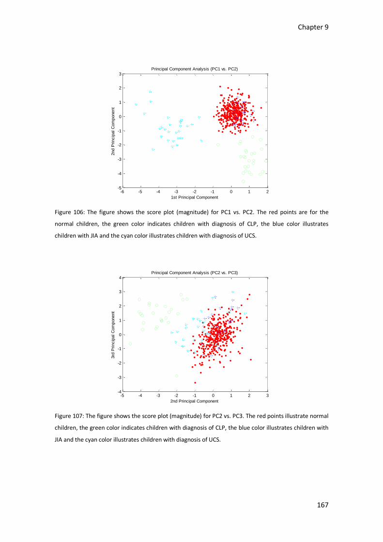
Chapter 9
167
Figure 106: The figure shows the score plot (magnitude) for PC1 vs. PC2. The red points are for the
normal children, the green color indicates children with diagnosis of CLP, the blue color illustrates
children with JIA and the cyan color illustrates children with diagnosis of UCS.
Figure 107: The figure shows the score plot (magnitude) for PC2 vs. PC3. The red points illustrate normal
children, the green color indicates children with diagnosis of CLP, the blue color illustrates children with
JIA and the cyan color illustrates children with diagnosis of UCS.
-6 -5 -4 -3 -2 -1 0 1 2-5
-4
-3
-2
-1
0
1
2
3
1st Principal Component
2nd P
rincip
al C
om
ponent
Principal Component Analysis (PC1 vs. PC2)
-5 -4 -3 -2 -1 0 1 2 3-4
-3
-2
-1
0
1
2
3
4
2nd Principal Component
3rd
Princip
al C
om
ponent
Principal Component Analysis (PC2 vs. PC3)

Chapter 9
168
The red points illustrate normal children, while the green color illustrates children with
diagnosis of CLP, the blue color illustrates children with JIA and the cyan color
illustrates children with diagnosis of UCS (Figures 106 and 107).
9.4.2.2 Principal Component mode plots
Figure 108 shows the five principal components modes in PCA model based on 451
faces (left column). The figures to the left illustrate five modes between -3 and +3
standard deviations from the mean. The green faces are the illustration for -3 standard
deviations, the blue faces are the mean symmetric face and the red faces are the
illustration for +3 standard deviations. Figure 108 (right column) show boxplots of the
same PC modes.
(a1) (a2)
(b1) (b2)
-80 -60 -40 -20 0 20 40 60 80-80
-60
-40
-20
0
20
40
x-values (mm)
y-v
alu
es (
mm
)
PC1 Mean- (blue), -3std-(green) and +3std face
-5
-4
-3
-2
-1
0
1
2
norm clp jia ucsType of faces
PC
1
PC1 for different face types
-80 -60 -40 -20 0 20 40 60 80-80
-60
-40
-20
0
20
40
x-values (mm)
y-v
alu
es (
mm
)
PC2 Mean- (blue), -3std-(green) and +3std face
-4
-3
-2
-1
0
1
2
norm clp jia ucsType of faces
PC
2
PC2 for different face types
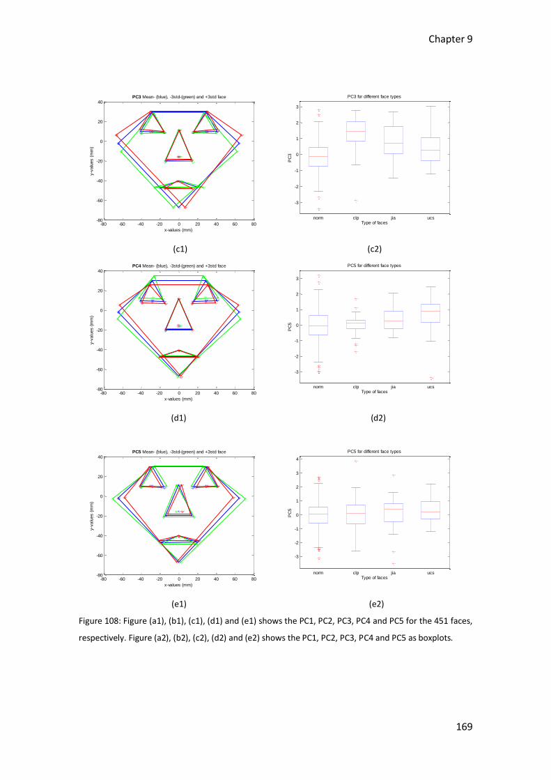
Chapter 9
169
(c1) (c2)
(d1) (d2)
(e1) (e2)
Figure 108: Figure (a1), (b1), (c1), (d1) and (e1) shows the PC1, PC2, PC3, PC4 and PC5 for the 451 faces,
respectively. Figure (a2), (b2), (c2), (d2) and (e2) shows the PC1, PC2, PC3, PC4 and PC5 as boxplots.
-80 -60 -40 -20 0 20 40 60 80-80
-60
-40
-20
0
20
40
x-values (mm)
y-v
alu
es (
mm
)
PC3 Mean- (blue), -3std-(green) and +3std face
-3
-2
-1
0
1
2
3
norm clp jia ucsType of faces
PC
3
PC3 for different face types
-80 -60 -40 -20 0 20 40 60 80-80
-60
-40
-20
0
20
40
x-values (mm)
y-v
alu
es (
mm
)
PC4 Mean- (blue), -3std-(green) and +3std face
-3
-2
-1
0
1
2
3
norm clp jia ucsType of faces
PC
5
PC5 for different face types
-80 -60 -40 -20 0 20 40 60 80-80
-60
-40
-20
0
20
40
x-values (mm)
y-v
alu
es (
mm
)
PC5 Mean- (blue), -3std-(green) and +3std face
-3
-2
-1
0
1
2
3
4
norm clp jia ucsType of faces
PC
5
PC5 for different face types
Chapter 9
170
9.5 Discussion
9.5.1 Asymmetry quantification
Figure 104 (a) shows the mean symmetric face and the mean normal face. These two
caricatures of faces look almost identical which means that the mean normal face
contains small amount of asymmetry.
Figure 104 (b) shows the mean symmetric face vs. the mean CLP face. Here it is
obvious that the upper lip is very asymmetric in relation to the mean symmetric face.
This can also be seen by means of Figure 100, which shows the amount of asymmetry
for the upper lip by means of boxplots. This is understandable since children with the
diagnosis of CLP have a very asymmetric nose and lip region.
In Figure 104 (c), it is seen that the children with the diagnosis of JIA look almost as
normal children except for the chin area; this is logical since these children are known
to develop asymmetric lower jaws due to inflammation in the jaw joint. Figure 101
shows boxplots for the asymmetry for the same area. A t-test reveals that the chin
area is very different between the normal faces and faces with the diagnosis of JIA.
Figure (d) shows bigger amount of asymmetry almost in the whole face in individuals
with UCS, especially in the eye and nasion area. Figure 102 shows boxplots of the
asymmetry for the eye outer corner where it is seen that the amount of asymmetry is
much bigger for the UCS. This is of course reasonable since these children are
diagnosed with the UCS, which means that one side of the forehead is prevented from
growing normally and thus remains flattened.
This is seen in Table 17 where the magnitude of asymmetry is seen to be largest in the
above mentioned areas for the different types of faces.

Chapter 9
171
9.5.2 Score and mode plots
Figure 106 shows a very good example of how the PCA separates different types of
craniofacial anomalies.
It is seen that PC1 is a mixture of many asymmetry locations (see Figure 108 (a1)). The
UCS is completely separated in PC1 even though many asymmetry types can be seen
for this component (see Figure 108 (a2)). This means that the UCS is very special with
regards to asymmetry.
This is not the case for JIA and CLP since the asymmetry is obvious in the upper
lip/nose area for the CLP and in the chin area for the JIA. This means that the
asymmetry is very local for both mentioned types of craniofacial anomalies and
therefore the asymmetry for these two types of disease is lost in the crowd of all other
types of asymmetry seen in PC1.
Figure 107 shows the PC2 vs. PC3. Here it is seen that CLP is separated from the normal
faces (see Figure 108 (b2)). Figure 107 can be compared to Figure 108 (b1) where the
mode plot (mode two) shows a big variation in the upper lip/nose area, which is as
expected. The score plot for PC3 (Figure 107) shows that JIA is placed more near the
edge when comparing with PC1 otherwise the PC3 does not give much contribution.
This score plot can be compared with Figure 108 (c1) where a bigger variation is seen
in the chin area, which is as expected due to the diagnosis of JIA.
9.6 Conclusion
In the present chapter the facial asymmetry has been quantified for 451 subjects. The
PCA has been applied to normal faces together with different types of craniofacial

Chapter 9
172
anomalies to demonstrate that PCA can distinguish between normal children and
different types of craniofacial anomalies by using the asymmetry quantification.
The score plots demonstrate the differences between the different types of faces (see
e.g. Figure 106).
The method may be used as a tool for identifying typical asymmetry-related features in
different types of craniofacial anomalies. Furthermore, it may be used for quantifying
the amount of these features (relative to a normal reference) that is present in a
patient, thus rendering it valuable as a tool in a clinical context.

Chapter 10
173
Chapter 10
Conclusion
In the present Thesis, a new methodology for quantification of facial asymmetry has
been developed and presented. The Thesis is concerned with quantifying asymmetry in
a large population (n=375) of normal children, thus providing reference values that can
be used e.g. for treatment purposes.
Quantification of asymmetry involved 1) determination of the MSP between the left
and right side of the face and 2) determination of corresponding anatomical locations
on left and right side, which was achieved by direct manual landmarking (Chapter 5
and 8), landmark-guided (Chapter 6) and automatic (Chapter 7) non-rigid registration
of a face surface to its mirror-surface.
In general, it was found that the critical task for quantification of asymmetry was the
method’s ability to accurately establishing anatomical point correspondences between
left and right side of the face.
Some of the major findings:
Mean facial asymmetry in the normal Caucasian population is 1.7 ± 0.9 mm.
Boys have a tendency to be more asymmetric than girls, but this is only
statistically significant in the chin region.
Asymmetry increases with age.
Asymmetry and its variation is not confined to, or dominated by, any particular
part of the face in normal children.

174
According to the result presented in Chapter 9, the asymmetry quantification can be
used as a diagnostic tool and it can for example discern between different phenotypes
of craniofacial anomalies. Asymmetry can also be used as a tool for quantification of
the severity of a particular disorder, and thereby be used in the context of treatment
progression monitoring and evaluation.

Bibliography
175
Bibliography
1. Eder, R.A. Craniofacial Anomalies Physiological Perspectives. Springer Verlag, St.
Louis and Washington, USA, 1995.
2. Jane J.A, Dumont A.S, Lin K.Y.K and Jane J.A Sr. Craniosynostosis. In: (Moore A.J,
Newell D.W, eds.) Neurosurgery: Principles and Practice. Springer, UK, USA, 2005.
3. Yamashita D.D.R, McAndrews J.P. Oral and Maxillofacial surgery clinics. USA, 2005.
4. Schroeder W, Martin K, Lorensen B. The Visualization Toolkit. 3rd Edition. Kitware,
USA, 2002.
5. Lanche S. Point-Wise Quantification of Craniofacial Asymmetry. Technical
University of Denmark (DTU), Lyngby, Denmark, 2007.
6. Hajnal J.V, Hill D.L.G, Hawkes D. J. Medical Image Registration. CRC Press LLC, USA,
2000.
7. Dryden I.L, Mardia K.V. Statistical Shape Analysis. John Wiley & Sons Ltd, UK, 1998.
8. Sonka M, Fitzpatrick J.M. Handbook of Medical Imaging – Volume 2. Medical
Image Processing and Analysis. Spie Press, USA, 2000.
9. Smith L.I. A tutorial on Principal Components Analysis. John Wiley & Sons Inc,
2002.
10. Speltz M.L, Kapp-Simon K.A, Cunningham M, Marsh J, Dawson G. Single-Suture
Craniosynostosis: A Review of Neurobehavioral Research and Theory. J. Pediatr.
Psychol. 2004; 29:651-668.
11. Murray JC. Gene/environmental causes of cleft lip and/or palate. Blackwell
Munksgaard, Clin Genet, 2002; 61:248-256.
12. Darvann TA, Hermann NV, Demant S, Larsen P, Ólafsdóttir, Thorup S, Zak M,
Lipira AB, Kane AA, Govier D, Schatz H, Rueckert D, Kreiborg S. In: Rueckert D.
(ed.) 2011 IEEE International Symposium on Biomedical Imaging: From Nano to
Macro, Chicago, IL, USA, March 30 – April 2, 2011. Pp. 1193-6.
13. Darvann TA, Ólafsdóttir H, Hermann NV, Larsen P, Lanche S, Larsen R, Ersbøll BK,
Govier D, Van Pelt AE, Kane AA, Hansen IV, Kreiborg S. On the measurement of
Bibliography
176
craniofacial asymmetry. In: K. Takada, S. Kreiborg (eds.) In Silico Dentistry – The
Evolution of Computational Oral Health Science. Osaka: Medigit, 2008, p. 37-41.
14. Klingenberg C.P, Barluenga M and Meyer A. Shape analysis of symmetric
structures: Quantifying variation among individuals and asymmetry. Evolution,
2002; 56:1909-20.
15. Darvann TA, Hermann NV, Larsen P, Ólafsdóttir H, Hansen IV, Hove HD,
Christensen L, Rueckert D, Kreiborg S. Automated quantification and analysis of
mandibular asymmetry. In: Niessen W, Meijering E (eds) Proceedings of IEEE
International Symposium on Biomedical Imaging: From Nano to Macro, Rotterdam
The Netherlands, 14-17 April 2010, pp. 416-9 (H; ISBN: 978-1-4244-4126-6; ISSN:
1945-7936).
16. Ólafsdóttir H, Lanche S, Darvann TA, Hermann NV, Larsen R, Ersbøll BK, Oubel E,
Frangi AF, Larsen P, Perlyn CA, Morriss-Kay GM, Kreiborg S. A point-wise
quantification of asymmetry using deformation fields: application to the study of
the Crouzon mouse model. Med Image Comput Comput Assist Interv (MICCAI)
2007;10:452-9.
17. Cheong YW, Lo LJ. Facial asymmetry: etiology, evaluation, and management. Chang
Gung Med J, 2011; 34:341-51.
18. Rasmussen M. Fluctuating asymmetry – indicator of what? Hereditas, 2002;
136:177-183.
19. Bates T.C. Fluctuating asymmetry and intelligence. Intelligence, 2007; 41-46.
20. Leung B, Forbes M.R. and Houle D. Fluctuating Asymmetry as a Bioindicator of
Stress: Comparing Efficacy of Analyses Involving Multiple Traits. The American
Naturalist, 2000; 101-115.
21. Leigh van Valen. A study of fluctuating asymmetry. Zoology Dept., Columbia
University, New York, Received July 5, 1961. p. 125-127.
22. Lipira AB, Sachanandani NS, Govier D, Payne A, Wyas S, Kleeschulte W, Kane AA.
Craniobank: an online collection of three-dimensional normative craniofacial
images. 2010; 126:70-72.
Bibliography
177
23. Demant S, Hermann N.V, Darvann T.A, Zak M, Schatz H, Larsen P. and Kreiborg S.
3D analysis of facial asymmetry in subjects with juvenile idiopathic arthritis.
Rheumatology, 2010.
24. Lanche S, Darvann T.A, Ólafsdóttir H, Hermann N.V, Van Pelt A.E, Govier D,
Tenenbaum M.J, Naidoo S, Larsen P, Kreiborg S, Larsen R and Kane A.A. A
statistical model of head asymmetry in infants with deformational plagiocephaly.
SCIA 2007; 4522:898-907.
25. Lipira A.B, Gordon S, Darvann T.A, Hermann N.V, Van Pelt A.E, Naidoo S.D, Govier
D. and Kane A.A. Helmet versus active repositioning for plagiocephaly: A three-
dimensional analysis. Pediatrics 2010; 126:e936.
26. Szeliski R. and Lavallée S. Matching 3D Anatomical Surfaces with Non-Rigid
Deformations using Octree-Splines. International Journal of Computer Vision (18)2,
171-186 (1996).
27. http://www.umm.edu/plasticsurgery/cranio.htm
28. http://upload.wikimedia.org/wikipedia/commons/1/1f/Single_suture_synostosis.p
ng
29. http://en.wikipedia.org/wiki/STL_(file_format)
30. http://www.craniofacial.net/conditions-craniosynostosis-coronal
31. http://support.sas.com/publishing/pubcat/chaps/55129.pdf
32. http://www.spineuniverse.com/anatomy/anatomical-planes-body
33. http://www.cleftbeforeafter.com/
34. http://www.newyorkfacialplasticsurgery.com/cleft-lip-and-cleft-palate-
surgery.html
35. http://my.clevelandclinic.org/disorders/rheumatoid_arthritis/hic_juvenile_idiopat
hic_arthritis.aspx
36. http://www.doc.ic.ac.uk/~dr/software/

178
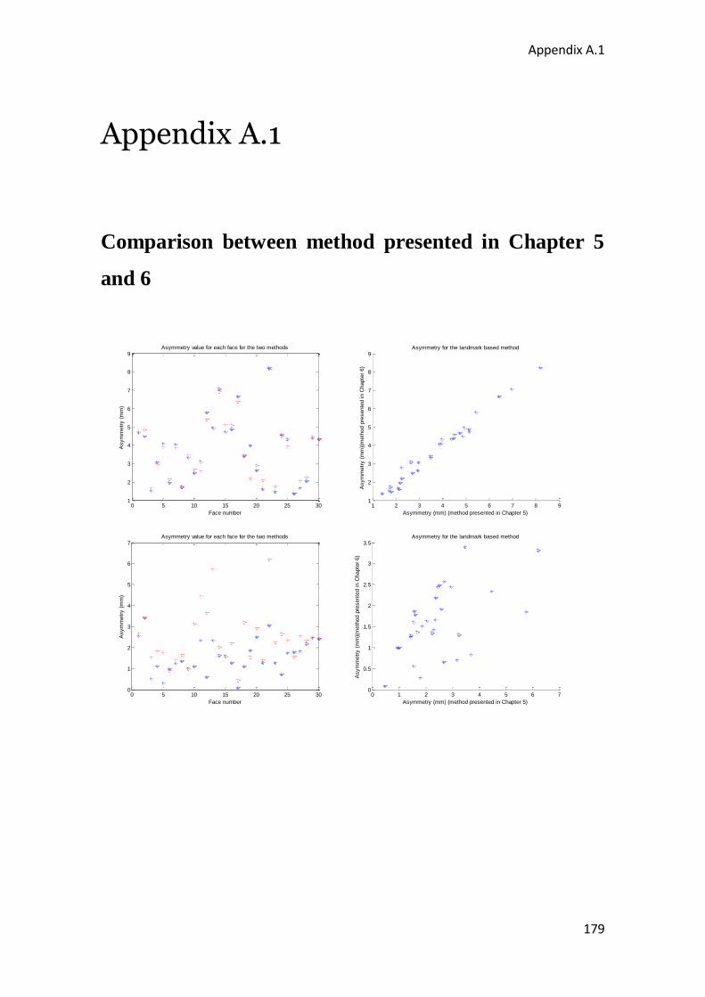
Appendix A.1
179
Appendix A.1
Comparison between method presented in Chapter 5
and 6
0 5 10 15 20 25 301
2
3
4
5
6
7
8
9
Face number
Asym
metr
y (
mm
)
Asymmetry value for each face for the two methods
1 2 3 4 5 6 7 8 91
2
3
4
5
6
7
8
9
Asymmetry (mm) (method presented in Chapter 5)
Asym
metr
y (
mm
)(m
eth
od p
resente
d in C
hapte
r 6)
Asymmetry for the landmark based method
0 5 10 15 20 25 300
1
2
3
4
5
6
7
Face number
Asym
metr
y (
mm
)
Asymmetry value for each face for the two methods
0 1 2 3 4 5 6 70
0.5
1
1.5
2
2.5
3
3.5
Asymmetry (mm) (method presented in Chapter 5)
Asym
metr
y (
mm
)(m
eth
od p
resente
d in C
hapte
r 6)
Asymmetry for the landmark based method
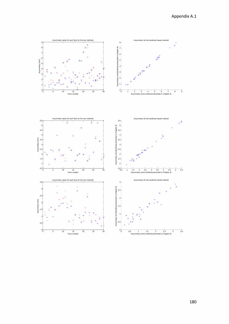
Appendix A.1
180
0 5 10 15 20 25 300
1
2
3
4
5
6
7
8
9
Face number
Asym
metr
y (
mm
)Asymmetry value for each face for the two methods
0 1 2 3 4 5 6 7 8 90
1
2
3
4
5
6
7
8
Asymmetry (mm) (method presented in Chapter 5)
Asym
metr
y (
mm
)(m
eth
od p
resente
d in C
hapte
r 6)
Asymmetry for the landmark based method
0 5 10 15 20 25 300.5
1
1.5
2
2.5
3
3.5
4
4.5
5
5.5
Face number
Asym
metr
y (
mm
)
Asymmetry value for each face for the two methods
0.5 1 1.5 2 2.5 3 3.5 4 4.5 5 5.50.5
1
1.5
2
2.5
3
3.5
4
4.5
5
5.5
Asymmetry (mm) (method presented in Chapter 5)
Asym
metr
y (
mm
)(m
eth
od p
resente
d in C
hapte
r 6)
Asymmetry for the landmark based method
0 5 10 15 20 25 300
0.5
1
1.5
2
2.5
3
3.5
Face number
Asym
metr
y (
mm
)
Asymmetry value for each face for the two methods
0 0.5 1 1.5 2 2.5 3 3.50
0.5
1
1.5
2
2.5
3
Asymmetry (mm) (method presented in Chapter 5)
Asym
metr
y (
mm
)(m
eth
od p
resente
d in C
hapte
r 6)
Asymmetry for the landmark based method
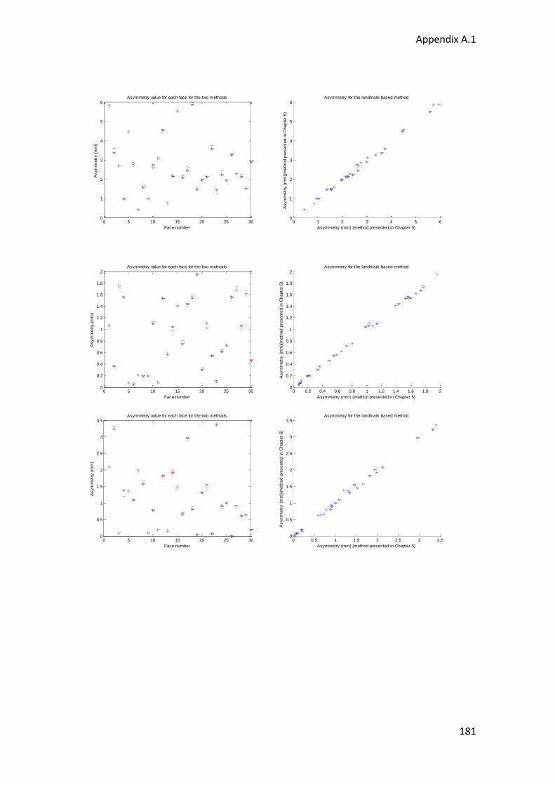
Appendix A.1
181
0 5 10 15 20 25 300
1
2
3
4
5
6
Face number
Asym
metr
y (
mm
)Asymmetry value for each face for the two methods
0 1 2 3 4 5 60
1
2
3
4
5
6
Asymmetry (mm) (method presented in Chapter 5)
Asym
metr
y (
mm
)(m
eth
od p
resente
d in C
hapte
r 6)
Asymmetry for the landmark based method
0 5 10 15 20 25 300
0.2
0.4
0.6
0.8
1
1.2
1.4
1.6
1.8
2
Face number
Asym
metr
y (
mm
)
Asymmetry value for each face for the two methods
0 0.2 0.4 0.6 0.8 1 1.2 1.4 1.6 1.8 20
0.2
0.4
0.6
0.8
1
1.2
1.4
1.6
1.8
2
Asymmetry (mm) (method presented in Chapter 5)
Asym
metr
y (
mm
)(m
eth
od p
resente
d in C
hapte
r 6)
Asymmetry for the landmark based method
0 5 10 15 20 25 300
0.5
1
1.5
2
2.5
3
3.5
Face number
Asym
metr
y (
mm
)
Asymmetry value for each face for the two methods
0 0.5 1 1.5 2 2.5 3 3.50
0.5
1
1.5
2
2.5
3
3.5
Asymmetry (mm) (method presented in Chapter 5)
Asym
metr
y (
mm
)(m
eth
od p
resente
d in C
hapte
r 6)
Asymmetry for the landmark based method

Appendix A.1
182
Figure 109: The left column shows the amount of asymmetry for each subject for the landmark based
method presented in Chapter 5 (blue) and Chapter 6 (red). The right column shows the asymmetry for
the method presented in Chapter 5 and 6 against each other.
0 5 10 15 20 25 300
0.5
1
1.5
2
2.5
3
3.5
Face number
Asym
metr
y (
mm
)
Asymmetry value for each face for the two methods
0 0.5 1 1.5 2 2.5 3 3.50
0.5
1
1.5
2
2.5
3
3.5
Asymmetry (mm) (method presented in Chapter 5)
Asym
metr
y (
mm
)(m
eth
od p
resente
d in C
hapte
r 6)
Asymmetry for the landmark based method

Appendix A.2
183
Appendix A.2
Comparison between method presented in Chapter 6
and 7
0 5 10 15 20 25 301
2
3
4
5
6
7
8
9
Face number
Asym
metr
y (
mm
)
Asymmetry for surface and landmark based method
1 2 3 4 5 6 7 8 91
2
3
4
5
6
7
Asymmetry (mm) (Landmark based method)
Asym
metr
y (
mm
) (S
urf
ace b
ased m
eth
od)
Asymmetry for surface and landmark based method against each other
0 5 10 15 20 25 300
1
2
3
4
5
6
7
Face number
Asym
metr
y (
mm
)
Asymmetry for surface and landmark based method
0 1 2 3 4 5 6 70.5
1
1.5
2
2.5
3
3.5
4
Asymmetry (mm) (Landmark based method)
Asym
metr
y (
mm
) (S
urf
ace b
ased m
eth
od)
Asymmetry for surface and landmark based method against each other
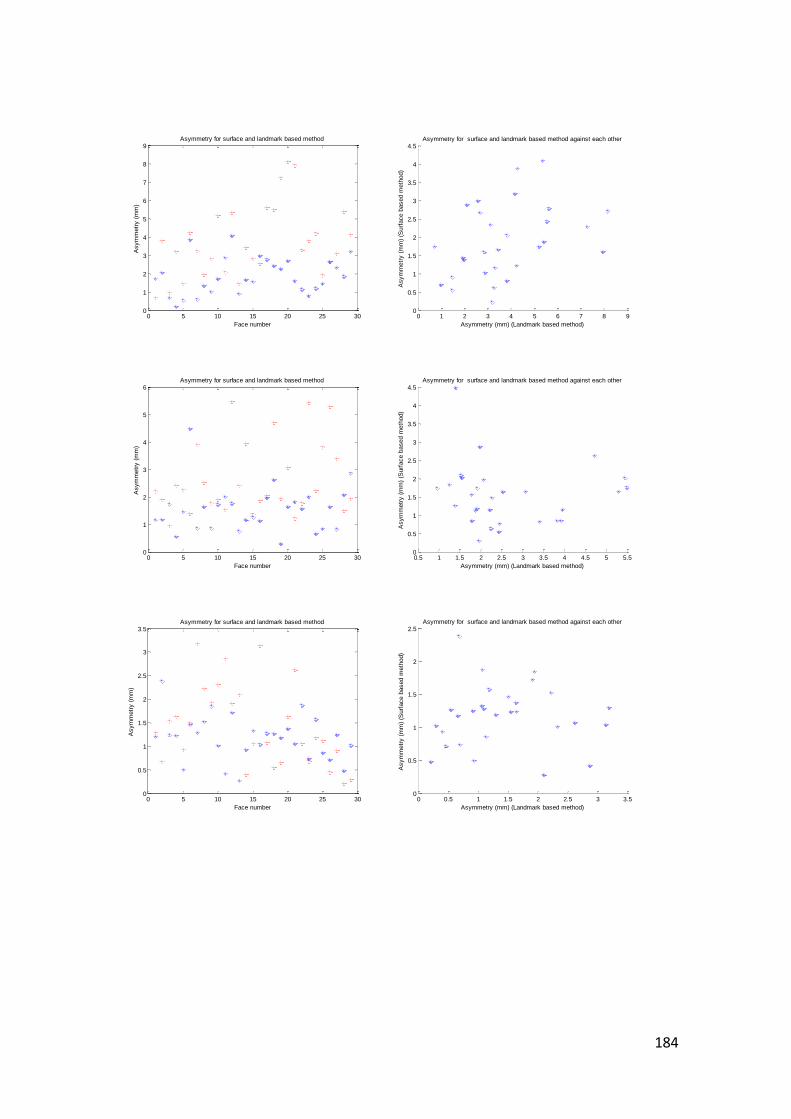
184
0 5 10 15 20 25 300
1
2
3
4
5
6
7
8
9
Face number
Asym
metr
y (
mm
)Asymmetry for surface and landmark based method
0 1 2 3 4 5 6 7 8 90
0.5
1
1.5
2
2.5
3
3.5
4
4.5
Asymmetry (mm) (Landmark based method)
Asym
metr
y (
mm
) (S
urf
ace b
ased m
eth
od)
Asymmetry for surface and landmark based method against each other
0 5 10 15 20 25 300
1
2
3
4
5
6
Face number
Asym
metr
y (
mm
)
Asymmetry for surface and landmark based method
0.5 1 1.5 2 2.5 3 3.5 4 4.5 5 5.50
0.5
1
1.5
2
2.5
3
3.5
4
4.5
Asymmetry (mm) (Landmark based method)
Asym
metr
y (
mm
) (S
urf
ace b
ased m
eth
od)
Asymmetry for surface and landmark based method against each other
0 5 10 15 20 25 300
0.5
1
1.5
2
2.5
3
3.5
Face number
Asym
metr
y (
mm
)
Asymmetry for surface and landmark based method
0 0.5 1 1.5 2 2.5 3 3.50
0.5
1
1.5
2
2.5
Asymmetry (mm) (Landmark based method)
Asym
metr
y (
mm
) (S
urf
ace b
ased m
eth
od)
Asymmetry for surface and landmark based method against each other

185
0 5 10 15 20 25 300
1
2
3
4
5
6
Face number
Asym
metr
y (
mm
)Asymmetry for surface and landmark based method
0 1 2 3 4 5 60.5
1
1.5
2
2.5
3
3.5
4
4.5
Asymmetry (mm) (Landmark based method)
Asym
metr
y (
mm
) (S
urf
ace b
ased m
eth
od)
Asymmetry for surface and landmark based method against each other
0 5 10 15 20 25 300
1
2
3
4
5
6
Face number
Asym
metr
y (
mm
)
Asymmetry for surface and landmark based method
0 0.2 0.4 0.6 0.8 1 1.2 1.4 1.6 1.8 20
1
2
3
4
5
6
Asymmetry (mm) (Landmark based method)
Asym
metr
y (
mm
) (S
urf
ace b
ased m
eth
od)
Asymmetry for surface and landmark based method against each other
0 5 10 15 20 25 300
0.5
1
1.5
2
2.5
3
3.5
Face number
Asym
metr
y (
mm
)
Asymmetry for surface and landmark based method
0 0.5 1 1.5 2 2.5 3 3.50
0.5
1
1.5
2
2.5
3
Asymmetry (mm) (Landmark based method)
Asym
metr
y (
mm
) (S
urf
ace b
ased m
eth
od)
Asymmetry for surface and landmark based method against each other
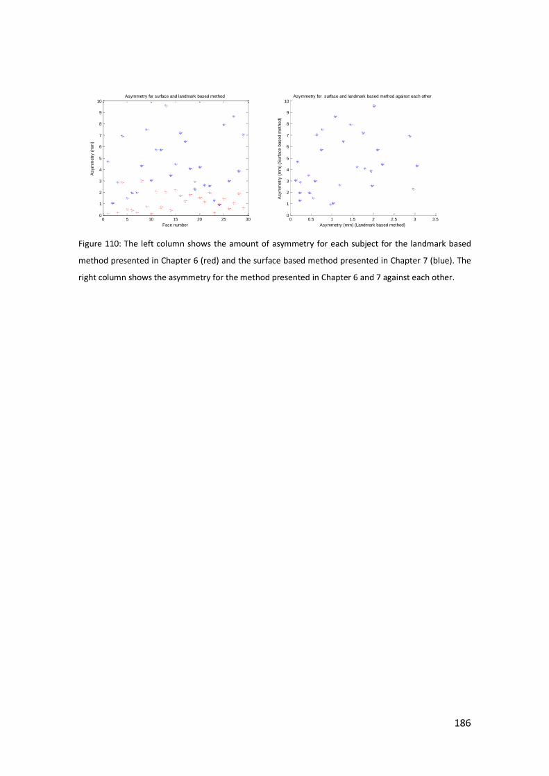
186
Figure 110: The left column shows the amount of asymmetry for each subject for the landmark based
method presented in Chapter 6 (red) and the surface based method presented in Chapter 7 (blue). The
right column shows the asymmetry for the method presented in Chapter 6 and 7 against each other.
0 5 10 15 20 25 300
1
2
3
4
5
6
7
8
9
10
Face number
Asym
metr
y (
mm
)
Asymmetry for surface and landmark based method
0 0.5 1 1.5 2 2.5 3 3.50
1
2
3
4
5
6
7
8
9
10
Asymmetry (mm) (Landmark based method)
Asym
metr
y (
mm
) (S
urf
ace b
ased m
eth
od)
Asymmetry for surface and landmark based method against each other
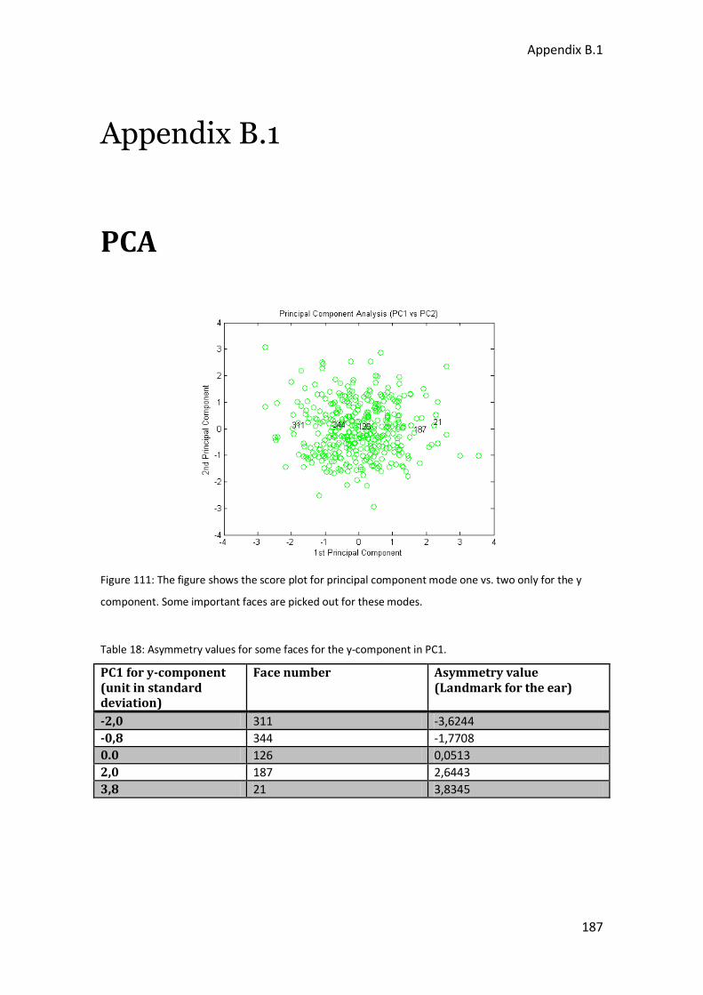
Appendix B.1
187
Appendix B.1
PCA
Figure 111: The figure shows the score plot for principal component mode one vs. two only for the y
component. Some important faces are picked out for these modes.
Table 18: Asymmetry values for some faces for the y-component in PC1.
PC1 for y-component (unit in standard deviation)
Face number Asymmetry value (Landmark for the ear)
-2,0 311 -3,6244
-0,8 344 -1,7708
0.0 126 0,0513
2,0 187 2,6443
3,8 21 3,8345
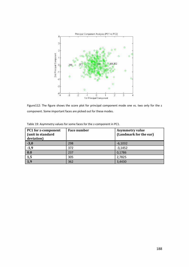
188
Figure112: The figure shows the score plot for principal component mode one vs. two only for the z
component. Some important faces are picked out for these modes.
Table 19: Asymmetry values for some faces for the z-component in PC1.
PC1 for z-component (unit in standard deviation)
Face number Asymmetry value (Landmark for the ear)
-3,0 298 -6,1032
-1,9 372 -3,1452
0.0 237 0,1786
1,5 305 2,7825
1,9 362 3,4430

189
Figure 113: Score plot for principal component mode one vs. two for the magnitude of asymmetry.
Table 20: Asymmetry (magnitude) values for some faces in PC1.
PC1 for the magnitude of asymmetry (unit in standard deviation)
Face number Asymmetry value (Landmark for the ear)
-2,8 49 x=1,6108 y=-2,7523 z=2,2583
-1,2 264 x=1,3787 y=-2,5904 z=1,6085
0.0 246 x=0,0515 y=0,1170 z=0,0067
1,7 210 x=-0,5170 y=2,0464 z=-2,2556
2,8 122 x=-0,4524 y=2,0824 z=-3,1560

190

Appendix C.1
191
Appendix C.1
Matlab scripts
Read files
This function read list files.
function [files_vtk,files_log,files_clr] =
read_list_file(infile_vtk,infile_log,infile_clr) % Reads a landmarker ascii log file (landmark file) files_vtk = textread(infile_vtk,'%s'); files_log = textread(infile_log,'%s'); files_clr = textread(infile_clr,'%s');
This function read log files.
function [lmarr,names,setarr] = read_log_file(infile_log) % Reads a landmarker ascii log file (landmark file) [x,y,z,names,setarr] = textread(infile_log,'%f%f%f%s%f'); lmarr = [x,y,z];
This function read clr files.
function p = readclr(infile_clr) %% Reads displacements from a clr file p =
textread(infile_clr,'%f','delimiter','\n','whitespace','','headerlines
',3);

192
This function read vtk files.
function data = readvtkpolydata(infile_vtk) %% check npoints [dum,npoints,dum] = textread(infile_vtk,'%s%d%s',1,'headerlines',4); %% points/triangles extrap = rem(npoints,3); %npoints = npoints-extrap; data.npoints = npoints; if extrap>0, extraline = 1; end tmp =
textread(infile_vtk,'%f',npoints*3,'headerlines',5,'delimiter','\n','w
hitespace',''); %data.points = reshape(tmp(1:end-extrap*3),[9 floor(npoints/3)])'; data.points = tmp;
%data.points = reshape(tmp,[9 npoints/3])'; %% polygons or vertices
linepos = 5+ceil(npoints/3); [text,n,dum] = textread(infile_vtk,'%s%d%d',1,'headerlines',linepos);
if strcmp(text,'POLYGONS') linepos = linepos+1; tmp =
textread(infile_vtk,'%d',n*4,'headerlines',linepos,'delimiter','\n','w
hitespace',''); data.poly = reshape(tmp,[4 n])'; data.npoly = n; data.ispoly = 1;
% ntot = 5+floor(npoints/3)+2+n; elseif strcmp(text,'VERTICES') linepos = linepos+1; tmp =
textread(infile_vtk,'%d',n*2,'headerlines',linepos,'delimiter','\n','w
hitespace',''); data.nvertices = n; data.vertices = reshape(tmp,[2 n])'; %ntot = 5+floor(npoints/3)+2+n; data.ispoly = 0; else error(['unknown format ',text]); end %% normals or not linepos = linepos+n+3; [text,dum,dum] =
textread(infile_vtk,'%s%s%s',1,'headerlines',linepos); if isempty(text) | strcmp(text,'NORMALS')==0 return else linepos = linepos+1; tmp =
textread(infile_vtk,'%f',npoints*3,'headerlines',linepos,'delimiter','
\n','whitespace',''); %data.normals = reshape(tmp(1:end-extrap*3),[9 npoints/3])';

193
%data.normals = reshape(tmp,[9 npoints/3])'; end
Load files
Files are loaded for the 30 faces used in Chapter 5.
infile_log='H:\yagmur\face_analyzer_position\listfile_log.txt'; %First
landmarking %infile_log='H:\yagmur\face_analyzer_position\listfile2.txt'; %Second %landmarking
[files_log] = read_list_file1(infile_log); nfiles = 30; numlm = 27; bigarr = zeros(numlm,3,nfiles); %3 tallet er x,y,z
for i = 1:nfiles file=sscanf(char(files_log(i)),'%s'); [lmarr,names,setarr] = read_log_file(file); bigarr(:,:,i)=lmarr; end n=20; for j=1:n for i=1:nfiles right(j,:,i)=bigarr(j,:,i); end end
Files are loaded for the 375 faces used in Chapter 8.
infile_log='H:\yagmur\face_analyzer_wm_wf\listfile_white.txt';
[files_log] = read_list_file1(infile_log); nfiles = 375; numlm = 26; bigarr = zeros(numlm,3,nfiles); %3 tallet er x,y,z
for i = 1:nfiles file=sscanf(char(files_log(i)),'%s'); [lmarr,names,setarr] = read_log_file(file); bigarr(:,:,i)=lmarr; end n=20; for j=1:n for i=1:nfiles right(j,:,i)=bigarr(j,:,i); end end

194
Files are loaded for the 451 faces used in Chapter 9.
infile_log='H:\yagmur\face_analyzer_wm_wf\listfile_white_all.txt'; [files_log] = read_list_file1(infile_log);
nfiles = 451; numlm = 26; bigarr = zeros(numlm,3,nfiles); %3 tallet er x,y,z
for i = 1:nfiles file=sscanf(char(files_log(i)),'%s'); % value=exist(file); % if (value == 0) % 'FEJL' % i % return % end [lmarr,names,setarr] = read_log_file(file); bigarr(:,:,i)=lmarr; end n=20; for j=1:n for i=1:nfiles right(j,:,i)=bigarr(j,:,i); end end
Centroid size
Centroid size is measured to make a size correction for the different faces since they
have different shapes.
%% Centroid size (CS) individer zero_point=right([10],:,:); %Assumed to be the midt point in the faces right=right([1 2 3 5 6 7 8 9 11 12 13 14 15 17 18 19 20],:,:); new_lm=17; % Measuring the ditance from the mean to all the other landmark points for % each face. cen_size = 0; for k=1:new_lm dist = zero_point - right(k); cen_size = cen_size + dist.*dist; end Cen_size = sqrt((1/new_lm)*cen_size);
%% CS template file_template=sscanf(char('H:\yagmur\face_analyzer_position\general\data\templ
ate_19_landmark.log'),'%s'); template = read_log_file(file_template); template=template([1 2 3 5 6 7 8 9 11 12 13 14 15 17 18 19 20],:,:);

195
zero_point_template=template([10],:,:);
cen_size_template=0; for k=1:new_lm dist_template = zero_point_template - template(k); cen_size_template = cen_size + dist.*dist; end Cen_size_template = sqrt((1/new_lm)*cen_size_template);
%% f=CS(template)/CS(individ) is quatified f=Cen_size_template./Cen_size;
Asymmetry quantification
Landmark based method
The Matlab script for the asymmetry quantification for the 30 subjects used in Chapter
5 is seen below.
%% Quantification of asymmetry
n=20; % The number of used landmarks
for j=1:n
for i=1:nfiles
right(j,:,i)=bigarr(j,:,i); % The landmark files are matrices of 20x3x30
end
end
left_mirror = right;
left_mirror(:,1,:)=right(:,1,:)*(-1); % Multiplying the x component by (-1) to
mirror it to the other side of MSP.
%The landmarks on the left and right side of the MSP are listed in order
according to the position of landmarks.
left_mirror=left_mirror([13 14 15 17 18 19 20 9 10 11 12 1 2 3 5 6 7 8],:,:);
right2=right([1 2 3 5 6 7 8 9 10 11 12 13 14 15 17 18 19 20],:,:);
%The asymmetry is quantified
asymmetry = right2-left_mirror;
%Only landmark 1:11 is choosen since they contain the nessasary for left and
right side
A = asymmetry([1 2 3 4 5 6 7 8 9 10 11],:,:);
%% Plotting x vs. y for the original landmark positions
R_x = right2(:,1,:);
R_y = right2(:,2,:);
R_z = right2(:,3,:);
%R_X = SQUEEZE(R_x) returns an array R_X with the same elements as R_x but
with all the singleton dimensions removed.
R_X = squeeze(R_x);

196
R_Y = squeeze(R_y);
R_Z = squeeze(R_z);
%Plotting
figure(1)
subplot(3,1,1)
plot(R_X,'*');
xlabel('Landmark number');
ylabel('x-values');
title('x, y and z values for landmarks');
subplot(3,1,2)
plot(R_Y,'*')
xlabel('Landmark number');
ylabel('y-values');
subplot(3,1,3)
plot(R_Z,'*')
xlabel('Landmark number');
ylabel('z-values');
figure(2)
plot(R_X,R_Y,'*');
xlabel('x-values');
ylabel('y-values');
title('Landmark position for x and y values of every face');
figure(3)
plot(R_X(:,1),R_Y(:,1),'*')
xlabel('x-values');
ylabel('y-values');
title('Landmark position for x and y values of one face');
%% Plotting x,y,z for the asymmetry vector
A_x = A(:,1,:);
A_y = A(:,2,:);
A_z = A(:,3,:);
X = squeeze(A_x);
Y = squeeze(A_y);
Z = squeeze(A_z);
figure(4)
subplot(3,1,1)
plot(X,'*');
xlabel('Landmark number');
ylabel('x-values');
title('x, y and z values of asymmetry of landmarks');
subplot(3,1,2)
plot(Y,'*')
xlabel('Landmark number');
ylabel('y-values');
subplot(3,1,3)
plot(Z,'*')
xlabel('Landmark number');
ylabel('z-values');
%% The average asymmetry for all faces and for all landmark points in all
faces is quantified:
%The length of asymmetry vector is found:
ASYM = sqrt(A(:,1,:).*A(:,1,:) + A(:,2,:).*A(:,2,:) + A(:,3,:).*A(:,3,:));
asym = squeeze(ASYM);
figure(5)
boxplot(asym);
ylim([-1 10]);
xlabel('Face number');

197
ylabel('Asymmetry (mm)');
title('Asymmetry of each face');
mean1 = mean(asym,1); % 1 stand for number of landmarks where each subject is
studied.
mean2 = mean(asym,2); % 2 stand for number of subjects for each subject where
each landmark point is studied.
SD1 = std(asym,0,1); % Subject
SD2 = std(asym,1,2); % Landmark point
MAX1 = max(asym,[],1);% Subject
MAX2 = max(asym,[],2);% Landmark point
MIN1 = min(asym,[],1);% Subject
MIN2 = min(asym,[],2);% Landmark point
figure(6)
subplot(2,2,1)
plot(mean1,'*');
xlabel('Face');
ylabel('Asymmetry (mm)');
title('Mean');
subplot(2,2,2)
plot(SD1,'*');
xlabel('Face');
ylabel('Asymmetry (mm)');
title('Standard deviation');
subplot(2,2,3)
plot(MAX1,'*');
xlabel('Face');
ylabel('Asymmetry (mm)');
title('Maximum value');
subplot(2,2,4)
plot(MIN1,'*');
xlabel('Face');
ylabel('Asymmetry (mm)');
title('Minimum value');
figure(7)
subplot(2,2,1)
plot(mean2,'*');
xlim([0 11]);
xlabel('Landmark number');
ylabel('Asymmetry (mm)');
title('Mean');
subplot(2,2,2)
plot(SD2,'*');
xlim([0 11]);
xlabel('Landmark number');
ylabel('Asymmetry (mm)');
title('Standard deviation');
subplot(2,2,3)
plot(MAX2,'*');
xlim([0 11]);
xlabel('Landmark number');
ylabel('Asymmetry (mm)');
title('Maximum value');
subplot(2,2,4)
plot(MIN2,'*');
xlim([0 11]);
xlabel('Landmark number');
ylabel('Asymmetry (mm)');
title('Minimum value');
%% Deviation from the mean is quantified
for i=1:29
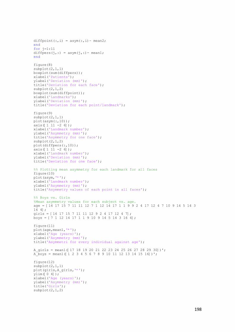
198
diffpoint(:,i) = asym(:,i)- mean2;
end
for j=1:11
diffpers(j,:) = asym(j,:)- mean1;
end
figure(8)
subplot(2,1,1)
boxplot(sum(diffpers));
xlabel('Patients');
ylabel('Deviation (mm)');
title('Deviation for each face');
subplot(2,1,2)
boxplot(sum(diffpoint));
xlabel('Landmarks');
ylabel('Deviation (mm)');
title('Deviation for each point/landmark');
figure(9)
subplot(2,1,1)
plot(asym(:,10));
axis([1 11 -2 6]);
xlabel('Landmark number');
ylabel('Asymmetry (mm)');
title('Asymmetry for one face');
subplot(2,1,2)
plot(diffpers(:,10));
axis([1 11 -2 6]);
xlabel('Landmark number');
ylabel('Deviation (mm)');
title('Deviation for one face');
%% Plotting mean asymmetry for each landmark for all faces
figure(10)
plot(asym,'*');
xlabel('Landmark number');
ylabel('Asymmetry (mm)');
title('Asymmetry values of each point in all faces');
%% Boys vs. Girls
%Mean asymmetry values for each subject vs. age.
age = [16 17 15 7 11 11 12 7 1 12 14 17 1 1 9 9 2 4 17 12 4 7 10 9 14 5 14 3
16 4];
girls = [16 17 15 7 11 11 12 9 2 4 17 12 4 7];
boys = [7 1 12 14 17 1 1 9 10 9 14 5 14 3 16 4];
figure(11)
plot(age,mean1,'*');
xlabel('Age (years)');
ylabel('Asymmetry (mm)');
title('Asymmetri for every individual against age');
A_girls = mean1([17 18 19 20 21 22 23 24 25 26 27 28 29 30])';
A_boys = mean1([1 2 3 4 5 6 7 8 9 10 11 12 13 14 15 16])';
figure(12)
subplot(2,1,1)
plot(girls,A_girls,'*');
ylim([0 4]);
xlabel('Age (years)');
ylabel('Asymmetry (mm)');
title('Girls');
subplot(2,1,2)
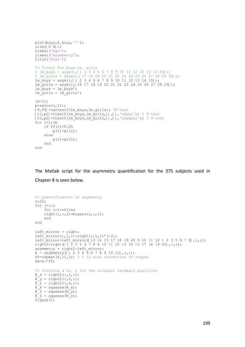
199
plot(boys,A_boys,'*');
ylim([0 4]);
xlabel('Age');
ylabel('Asymmetry');
title('Boys');
%% T-test for boys vs. girls
% lm_boys = asym(:,[1 2 3 4 5 6 7 8 9 10 11 12 13 14 15 16]);
% lm_girls = asym(:,[17 18 19 20 21 22 23 24 25 26 27 28 29 30]);
lm_boys = asym(:,[1 2 3 4 5 6 7 8 9 10 11 12 13 14 15]);
lm_girls = asym(:,[16 17 18 19 20 21 22 23 24 25 26 27 28 29]);
lm_boys = lm_boys';
lm_girls = lm_girls';
lm=11;
p=zeros(1,11);
[H,Pf]=vartest2(lm_boys,lm_girls); %F-test
[t1,p1]=ttest2(lm_boys,lm_girls,[],[],'equal'); % T-test
[t2,p2]=ttest2(lm_boys,lm_girls,[],[],'unequal'); % T-test
for i=1:lm
if Pf(i)<0.05
p(i)=p1(i);
else
p(i)=p2(i);
end
end
The Matlab script for the asymmetry quantification for the 375 subjects used in
Chapter 8 is seen below.
%% Quantification of asymmetry n=20; for j=1:n for i=1:nfiles right(j,:,i)=bigarr(j,:,i); end end
left_mirror = right; left_mirror(:,1,:)=right(:,1,:)*(-1); left_mirror=left_mirror([13 14 15 17 18 19 20 9 10 11 12 1 2 3 5 6 7 8],:,:); right2=right([1 2 3 5 6 7 8 9 10 11 12 13 14 15 17 18 19 20],:,:); asymmetry = right2-left_mirror; A = asymmetry([1 2 3 4 5 6 7 8 9 10 11],:,:); ff=repmat(f,11,1); % f is size correction of shapes AA=A.*ff;
%% Plotting x vs. y for the original landmark positions R_x = right2(:,1,:); R_y = right2(:,2,:); R_z = right2(:,3,:); R_X = squeeze(R_x); R_Y = squeeze(R_y); R_Z = squeeze(R_z); figure(1)

200
subplot(3,1,1) plot(R_X,'*'); xlabel('Landmark number'); ylabel('x-values'); title('x, y and z values for landmarks'); subplot(3,1,2) plot(R_Y,'*') xlabel('Landmark number'); ylabel('y-values'); subplot(3,1,3) plot(R_Z,'*') xlabel('Landmark number'); ylabel('z-values'); figure(2) plot(R_X,R_Y,'*'); xlabel('x-values'); ylabel('y-values'); title('Landmark position for x and y values of every face');
%% Plotting x,y,z for the asymmetry vector A_x = AA(:,1,:); A_y = AA(:,2,:); A_z = AA(:,3,:); X = squeeze(A_x); Y = squeeze(A_y); Z = squeeze(A_z);
figure(4) subplot(3,1,1) plot(X,'*'); xlabel('Landmark number'); ylabel('x-values'); title('x, y and z values of asymmetri of landmarks'); subplot(3,1,2) plot(Y,'*') xlabel('Landmark number'); ylabel('y-values'); subplot(3,1,3) plot(Z,'*') xlabel('Landmark number'); ylabel('z-values'); %% The average asymmetry for all faces and for all landmark points in all
faces are quantified: %The lenght of asymmetry vector is found: ASYM = sqrt(AA(:,1,:).*AA(:,1,:) + AA(:,2,:).*AA(:,2,:) +
AA(:,3,:).*AA(:,3,:)); asym = squeeze(ASYM);
%Plotting box plots for 375 subjects figure(55) subplot(5,2,1) boxplot(asym,'plotstyle','compact'); xlim([1 37]); ylabel('Asymmetry (mm)','FontSize',5); title('Asymmetry of each face'); subplot(5,2,2) boxplot(asym,'plotstyle','compact'); xlim([38 75]); ylabel('Asymmetry (mm)','FontSize',5); title('Asymmetry of each face'); subplot(5,2,3) boxplot(asym,'plotstyle','compact');
201
xlim([76 113]); ylabel('Asymmetry (mm)','FontSize',5); subplot(5,2,4) boxplot(asym,'plotstyle','compact'); xlim([114 150]); ylabel('Asymmetry (mm)','FontSize',5); subplot(5,2,5) boxplot(asym,'plotstyle','compact'); xlim([151 187]); ylabel('Asymmetry (mm)','FontSize',5); subplot(5,2,6) boxplot(asym,'plotstyle','compact'); xlim([188 225]); ylabel('Asymmetry (mm)','FontSize',5); subplot(5,2,7) boxplot(asym,'plotstyle','compact'); xlim([226 263]); ylabel('Asymmetry (mm)','FontSize',5); subplot(5,2,8) boxplot(asym,'plotstyle','compact'); xlim([264 301]); ylabel('Asymmetry (mm)','FontSize',5); subplot(5,2,9) boxplot(asym,'plotstyle','compact'); xlim([302 339]); xlabel('Face number','FontSize',10); ylabel('Asymmetry (mm)','FontSize',5); subplot(5,2,10) boxplot(asym,'plotstyle','compact'); xlim([340 375]); xlabel('Face number','FontSize',10); ylabel('Asymmetry (mm)','FontSize',5);
mean1 = mean(asym,1); % 1 står for antal landmarks, hvor hvert individ
undersøges. mean2 = mean(asym,2); % 2 står for antal individer, hvor hvert punkt
undersøges. SD1 = std(asym,0,1); % individ SD2 = std(asym,1,2); % punkt MAX1 = max(asym,[],1);% individ MAX2 = max(asym,[],2);% punkt MIN1 = min(asym,[],1);% individ MIN2 = min(asym,[],2);% punkt
figure(6) subplot(2,2,1) plot(mean1,'*'); xlabel('Face number'); ylabel('Asymmetry (mm)'); title('Mean'); subplot(2,2,2) plot(SD1,'*'); xlabel('Face number'); ylabel('Asymmetry (mm)'); title('Standard deviation'); subplot(2,2,3) plot(MAX1,'*'); xlabel('Face number'); ylabel('Asymmetry (mm)'); title('Maximum value'); subplot(2,2,4) plot(MIN1,'*');
202
xlabel('Face number'); ylabel('Asymmetry (mm)'); title('Minimum value');
figure(7) subplot(2,2,1) plot(mean2,'*'); xlim([0 11]); xlabel('Landmark number'); ylabel('Asymmetry (mm)'); title('Mean'); subplot(2,2,2) plot(SD2,'*'); xlim([0 11]); xlabel('Landmark number'); ylabel('Asymmetry (mm)'); title('Standard deviation'); subplot(2,2,3) plot(MAX2,'*'); xlim([0 11]); xlabel('Landmark number'); ylabel('Asymmetry (mm)'); title('Maximum value'); subplot(2,2,4) plot(MIN2,'*'); xlim([0 11]); xlabel('Landmark number'); ylabel('Asymmetry (mm)'); title('Minimum value'); %% Deviation from the mean is quantified for i=1:30 diffpoint(:,i) = asym(:,i)- mean2; end for j=1:11 diffpers(j,:) = asym(j,:)- mean1; end
figure(8) subplot(2,1,1) boxplot(sum(diffpers)); xlabel('Faces'); ylabel('Deviation'); title('Deviation for each face'); subplot(2,1,2) boxplot(sum(diffpoint)); xlabel('Landmarks'); ylabel('Deviation'); title('Deviation for each point/landmark'); %% Plotting mean asymmetry for each landmark for all faces figure(9) plot(asym,'*'); xlabel('Landmark number'); ylabel('Asymmetry (mm)'); title('Asymmetri values of each point in all faces');
%% Age WM=[116 110 162 61 162 188 52 6 42 27 48 103 122 45 119 48 28 88 93 51 122 15 81 100 127 122 120 75 81 24 126 90 158
113 128 121 43 196 47 209 45 100 91 2 52 151 144 3 109 127 158 68 50 186 49 133 42 57 78 72 18 144 145 189 137 37 61
70 114 133 178 130 53 62 13 162 102 142 35 109 15 142 141 84 52 145 122 2 29 112 35 162 41 8 193 96 17 177 86 189 16
152 163 124 14 114 75 27 4 91 43 61 36 70 115 152 89 138 43 58 37 134 76 114 158 111 58 71 59 142 214 40 73 208 51 49
87 128 44 7 53 118 220 70 184 13 21 62 118 51 65 111 141 40 84 83 111 187 49 60 172 104 117 144 6 64 204 6 81 105 54
71 61 168 52 210 20 83 101 48 16 23 24 1 109 14 9 80 57 65 39 145 142 92 96 67 109 125 116 18 104 42 34 44 151 62 95
25 142 88 72 50]; WF=[112 25 53 205 146 52 86 108 195 175 87 145 169 75 27 106 137 74 95 138 63 126 147 191 49 159 8 15 173 39 10 37 51
140 24 36 167 184 47 108 12 16 105 42 40 15 15 27 2 186 9 4 35 20 24 90 152 208 129 184 4 44 66 66 125 2 120 105 36

203
156 48 61 89 124 80 114 171 34 151 178 142 149 116 25 103 51 171 53 78 39 154 111 82 158 169 170 104 76 1 140 76 28 97
161 85 51 25 157 21 141 129 109 127 60 198 122 105 76 12 201 39 82 144 176 96 9 89 144 218 64 196 8 67 137 90 104 114
107 118 125 113 153 55 137 162 65 62 66 95 46 85 188 38 62 103 30 88 67 116 160 146 146 190];
wm=WM/12; %Age in year wf=WF/12; %Age in year wmx = mean1([1 2 3 6 8 11 12 13 14 16 19 20 23 25 26 27 29 30 32 33 35 36 38 41 42 45 47 48 49 51 52 53 54 55 57 62 65
66 67 68 70 71 73 76 77 79 81 82 86 88 90 93 94 100 101 102 104 113 114 115 116 117 120 122 124 126 127 129 130 131
132 136 138 140 141 142 143 146 148 149 151 152 153 154 155 156 157 159 161 162 163 164 166 167 168 172 174 176 177
180 181 182 183 184 188 190 193 195 196 197 198 199 200 202 203 204 205 206 207 208 209 212 214 215 216 218 220 221
222 223 227 230 231 232 233 234 236 237 239 241 244 246 247 249 250 254 255 256 257 259 260 261 262 264 268 269 271
274 275 277 279 282 284 286 288 289 290 292 294 295 296 299 300 301 302 303 306 307 308 309 315 316 317 318 319 320
321 322 324 325 326 327 328 329 332 333 335 341 342 343 345 346 349 351 353 355 361 262 364 365 366 367]); wfx = mean1([4 5 7 9 10 15 17 18 21 22 24 28 31 34 37 39 40 43 44 46 50 56 58 59 60 61 63 64 69 72 74 75 78 80 83 84
85 87 89 91 92 95 96 97 98 99 103 105 106 107 108 109 110 111 112 118 119 121 123 125 128 133 134 135 137 139 144 145
147 150 158 160 165 169 170 171 173 175 178 179 185 186 187 189 191 192 194 201 210 211 213 217 219 224 225 226 228
229 235 238 240 242 243 245 248 251 252 253 258 263 265 266 267 270 272 273 276 278 280 281 283 285 287 291 293 297
298 304 305 310 311 312 313 314 323 330 331 334 336 337 338 339 340 344 347 348 350 352 354 356 357 358 359 360 363
368 369 370 371 372 373 374 375]);
figure(111) subplot(2,1,1); hist(wm,212); axis ([0 19 0 6]) xlabel('Age in years') ylabel('Number of subjects') title ('Age of boys') subplot(2,1,2); hist(wf,163); axis ([0 19 0 6]) xlabel('Age in years') ylabel('Number of subjects') title ('Age of girls')
figure(12) subplot(2,1,1) plot(wf,wfx,'*'); xlabel('Age (years)'); ylabel('Asymmetry (mm)'); title('Girls'); subplot(2,1,2) plot(wm,wmx,'*'); xlabel('Age (years)'); ylabel('Asymmetry (mm)'); title('Boys');
figure (13) plot(wf,wfx,'*r'); hold on plot(wm,wmx,'*b'); xlabel('Age(years)'); ylabel('Asymmetry (mm)'); title('Boys and Girls');
%% T-test lm_boys = asym(:,[1 2 3 6 8 11 12 13 14 16 19 20 23 25 26 27 29 30 32 33 35 36 38 41 42 45 47 48 49 51 52 53 54 55 57
62 65 66 67 68 70 71 73 76 77 79 81 82 86 88 90 93 94 100 101 102 104 113 114 115 116 117 120 122 124 126 127 129 130
131 132 136 138 140 141 142 143 146 148 149 151 152 153 154 155 156 157 159 161 162 163 164 166 167 168 172 174 176
177 180 181 182 183 184 188 190 193 195 196 197 198 199 200 202 203 204 205 206 207 208 209 212 214 215 216 218 220
221 222 223 227 230 231 232 233 234 236 237 239 241 244 246 247 249 250 254 255 256 257 259 260 261 262 264 268 269
271 274 275 277 279 282 284 286 288 289 290 292 294 295 296 299 300 301 302 303 306 307 308 309 315 316 317 318 319
320 321 322 324 325 326 327 328 329 332 333 335 341 342 343 345 346 349 351 353 355 361 262 364 365 366 367]); lm_girls = asym(:,[4 5 7 9 10 15 17 18 21 22 24 28 31 34 37 39 40 43 44 46 50 56 58 59 60 61 63 64 69 72 74 75 78 80
83 84 85 87 89 91 92 95 96 97 98 99 103 105 106 107 108 109 110 111 112 118 119 121 123 125 128 133 134 135 137 139
144 145 147 150 158 160 165 169 170 171 173 175 178 179 185 186 187 189 191 192 194 201 210 211 213 217 219 224 225
226 228 229 235 238 240 242 243 245 248 251 252 253 258 263 265 266 267 270 272 273 276 278 280 281 283 285 287 291
293 297 298 304 305 310 311 312 313 314 323 330 331 334 336 337 338 339 340 344 347 348 350 352 354 356 357 358 359
360 363 368 369 370 371 372 373 374 375]);
lm_boys = lm_boys'; lm_girls = lm_girls';
figure(14)

204
boxplot(asym'); xlabel('Landmark number'); ylabel('Asymmetry (mm)'); title('Asymmetry of each face in different points');
lm=11; p=zeros(1,11); [H,Pf]=vartest2(lm_boys,lm_girls); %F-test [t1,p1]=ttest2(lm_boys,lm_girls,[],[],'equal'); % T-test [t2,p2]=ttest2(lm_boys,lm_girls,[],[],'unequal'); % T-test for i=1:lm if Pf(i)<0.05 p(i)=p1(i); else p(i)=p2(i); end end
%% Figure shows the landmarks for chin for each face figure(14) subplot(2,1,1) plot(lm_boys(:,11),'*'); xlabel('Boys'); ylabel('Asymmetry (mm)'); ylim([0 6]); title('Chin of each face'); hold on subplot(2,1,2) plot(lm_girls(:,11),'*'); xlabel('Girls'); ylabel('Asymmetry (mm)'); ylim([0 6]); title('Chin of each face');
%% Dividing boys and girls in young (0-9 years old) and old (10-18 years old)
boys and girls. %Boys boys_young=WM(find(WM<=108)); boys_old=WM(find(WM>108)); boys_young=boys_young/12; boys_old=boys_old/12;
boys_asym_young=asym(:,[6 12 13 14 16 19 23 26 27 29 30 32 35 36 38 47 48 49 55 67 70 71 73 76 77 82 93 94 101 104 113
114 115 120 127 129 131 136 138 140 141 143 148 151 154 155 159 161 163 166 167 172 174 177 181 182 183 190 193 195
196 197 198 199 200 204 207 209 216 218 220 223 227 231 232 233 236 237 239 246 249 250 254 256 260 261 262 269 271
275 279 282 284 286 288 290 292 294 295 296 299 301 303 307 308 309 315 316 317 318 320 321 322 324 325 326 329 332
333 343 345 346 349 351 355 361 262 365 366 367]); %0 boys_asym_old=asym(:,[1 2 3 8 11 20 25 33 41 42 45 51 52 53 54 57 62 65 66 68 79 81 86 88 90 100 102 116 117 122 124
126 130 132 142 146 149 152 153 156 157 162 164 168 176 180 184 188 202 203 205 206 208 212 214 215 221 222 230 234
241 244 247 255 257 259 264 268 274 277 289 300 302 306 319 327 328 335 341 342 353 364]); %1
boys_asym_young=boys_asym_young'; boys_asym_old=boys_asym_old'; boys_mean_young=mean1([6 12 13 14 16 19 23 26 27 29 30 32 35 36 38 47 48 49 55 67 70 71 73 76 77 82 93 94 101 104 113
114 115 120 127 129 131 136 138 140 141 143 148 151 154 155 159 161 163 166 167 172 174 177 181 182 183 190 193 195
196 197 198 199 200 204 207 209 216 218 220 223 227 231 232 233 236 237 239 246 249 250 254 256 260 261 262 269 271
275 279 282 284 286 288 290 292 294 295 296 299 301 303 307 308 309 315 316 317 318 320 321 322 324 325 326 329 332
333 343 345 346 349 351 355 361 262 365 366 367]); %0 boys_mean_old=mean1([1 2 3 8 11 20 25 33 41 42 45 51 52 53 54 57 62 65 66 68 79 81 86 88 90 100 102 116 117 122 124
126 130 132 142 146 149 152 153 156 157 162 164 168 176 180 184 188 202 203 205 206 208 212 214 215 221 222 230 234
241 244 247 255 257 259 264 268 274 277 289 300 302 306 319 327 328 335 341 342 353 364]); %1
lm=11; p_boys=zeros(1,11); [H1,Pf1]=vartest2(boys_asym_young,boys_asym_old); %F-test [t12,p12]=ttest2(boys_asym_young,boys_asym_old,[],[],'equal'); % T-test [t21,p21]=ttest2(boys_asym_young,boys_asym_old,[],[],'unequal'); % T-test for i=1:lm

205
if Pf1(i)<0.05 p_boys(i)=p12(i); else p_boys(i)=p21(i); end end
%Plotter asymmetri værdier for landmark nr. 8 figure(15) subplot(2,1,1) plot(boys_asym_young(:,8),'*'); xlabel('Boys (landmark of the nasion)'); ylabel('Asymmetry (mm)'); ylim([0 5]); title('Young boys (0-9 years)'); hold on subplot(2,1,2) plot(boys_asym_old(:,8),'*'); ylim([0 5]); xlabel('Boys (landmark of the nasion)'); ylabel('Asymmetry (mm)'); title('Old boys (10-18 years)');
figure(16) subplot(2,1,1) plot(boys_young,boys_mean_young,'*'); xlabel('Age (years)'); ylabel('Asymmetry (mm)'); title('Young boys (0-9years)'); hold on subplot(2,1,2) plot(boys_old,boys_mean_old,'*'); xlabel('Age (years)'); ylabel('Asymmetry (mm)'); title('Old boys (10-18 years)');
%Girls girls_young=WF(find(WF<=108)); girls_old=WF(find(WF>108)); girls_young=girls_young/12; girls_old=girls_old/12;
lm_girls = asym(:,[4 5 7 9 10 15 17 18 21 22 24 28 31 34 37 39 40 43 44 46 50 56 58 59 60 61 63 64 69 72 74 75 78 80
83 84 85 87 89 91 92 95 96 97 98 99 103 105 106 107 108 109 110 111 112 118 119 121 123 125 128 133 134 135 137 139
144 145 147 150 158 160 165 169 170 171 173 175 178 179 185 186 187 189 191 192 194 201 210 211 213 217 219 224 225
226 228 229 235 238 240 242 243 245 248 251 252 253 258 263 265 266 267 270 272 273 276 278 280 281 283 285 287 291
293 297 298 304 305 310 311 312 313 314 323 330 331 334 336 337 338 339 340 344 347 348 350 352 354 356 357 358 359
360 363 368 369 370 371 372 373 374 375]); girls_asym_young=asym(:,[5 7 15 17 18 24 34 37 39 43 44 50 60 63 64 72 74 75 78 83 84 89 91 92 95 96 97 98 99 103 105
106 108 109 110 111 112 118 128 133 134 135 139 145 147 158 160 165 170 175 189 191 192 201 210 211 219 228 229 235
240 242 243 248 251 252 258 270 276 278 280 283 285 293 297 298 310 312 313 323 330 334 340 348 350 352 354 356 357
359 360 363 368 369 370]); girls_asym_old=asym(:,[4 9 10 21 22 28 31 40 46 56 58 59 61 69 80 85 87 107 119 121 123 125 137 144 150 169 171 173
178 179 185 186 187 194 213 217 224 225 226 238 245 253 263 265 266 267 272 273 281 287 291 304 305 311 314 331 336
337 338 339 344 347 358 371 372 373 374 375]); girls_asym_young=girls_asym_young'; girls_asym_old=girls_asym_old'; girls_mean_young=mean1(:,[5 7 15 17 18 24 34 37 39 43 44 50 60 63 64 72 74 75 78 83 84 89 91 92 95 96 97 98 99 103 105
106 108 109 110 111 112 118 128 133 134 135 139 145 147 158 160 165 170 175 189 191 192 201 210 211 219 228 229 235
240 242 243 248 251 252 258 270 276 278 280 283 285 293 297 298 310 312 313 323 330 334 340 348 350 352 354 356 357
359 360 363 368 369 370]); girls_mean_old=mean1(:,[4 9 10 21 22 28 31 40 46 56 58 59 61 69 80 85 87 107 119 121 123 125 137 144 150 169 171 173
178 179 185 186 187 194 213 217 224 225 226 238 245 253 263 265 266 267 272 273 281 287 291 304 305 311 314 331 336
337 338 339 344 347 358 371 372 373 374 375]);
lm=11; p_girls=zeros(1,11); [H2,Pf2]=vartest2(girls_asym_young,girls_asym_old); %F-test [t13,p13]=ttest2(girls_asym_young,girls_asym_old,[],[],'equal'); % T-test

206
[t31,p31]=ttest2(girls_asym_young,girls_asym_old,[],[],'unequal'); % T-test for i=1:lm if Pf1(i)<0.05 p_girls(i)=p13(i); else p_girls(i)=p31(i); end end
%Plotter asymmetri værdier for landmark nr. 8 figure(17) subplot(2,1,1) plot(girls_asym_young(:,8),'*'); xlabel('Girls (landmark of the nasion)'); ylabel('Asymmetry (mm)'); ylim([0 5]); title('Young girls (0-9 years)'); hold on subplot(2,1,2) plot(girls_asym_old(:,8),'*'); xlabel('Girls (landmark of the nasion)'); ylabel('Asymmetry (mm)'); ylim([0 5]); title('Old girls (10-18 years)');
figure(18) subplot(2,1,1) plot(girls_young,girls_mean_young,'*'); xlabel('Age (years)'); ylabel('Asymmetry (mm)'); ylim([0 4]); title('Young girls (0-9 years)'); hold on subplot(2,1,2) plot(girls_old,girls_mean_old,'*'); xlabel('Age (years)'); ylabel('Asymmetry (mm)'); ylim([0 4]); title('Old girls (10-18 years)'); %% Difference between boys and girls in age 0-9 and 10-18 %Young lm=11; p_1=zeros(1,11); [H_1,Pf_1]=vartest2(girls_asym_young,boys_asym_young); %F-test [t_11,p_11]=ttest2(girls_asym_young,boys_asym_young,[],[],'equal'); % T-test [t_12,p_12]=ttest2(girls_asym_young,boys_asym_young,[],[],'unequal'); % T-test for i=1:lm if Pf_1(i)<0.05 p_1(i)=p_11(i); else p_1(i)=p_12(i); end end %Old lm=11; p_2=zeros(1,11); [H_2,Pf_2]=vartest2(girls_asym_old,boys_asym_old); %F-test [t_21,p_21]=ttest2(girls_asym_old,boys_asym_old,[],[],'equal'); % T-test [t_22,p_22]=ttest2(girls_asym_old,boys_asym_old,[],[],'unequal'); % T-test for i=1:lm if Pf_2(i)<0.05 p_2(i)=p_21(i);

207
else p_2(i)=p_22(i); end end
Face Analyzer
Below the Matlab script for the files used in the software program Face analyzer is
seen. The amount of asymmetry is quantified by this Matlab script.
%% Loading vtk, log and clr files infile_vtk='H:\yagmur\face_analyzer_position\listfile_vtk.txt'; infile_log='H:\yagmur\face_analyzer_position\listfile_log.txt'; infile_clr='H:\yagmur\face_analyzer_position\listfile_diff_face.txt';
[files_vtk,files_log,files_clr] =
read_list_file(infile_vtk,infile_log,infile_clr);
nfiles = 30; n_landm = 18; all_index = zeros(n_landm,nfiles); asym_arr = zeros(n_landm,nfiles); for i = 1:nfiles vtk_arr=readvtkpolydata(char(files_vtk(i))); log_arr_all=read_log_file(char(files_log(i))); log_arr = log_arr_all([1 2 3 5 6 7 8 9 10 11 12 13 14 15 17 18 19 20],:); clr_arr=readclr(char(files_clr(i))); index_arr = find_index(vtk_arr,log_arr,clr_arr); all_index(:,i) = index_arr; asym_arr(:,i) = clr_arr(index_arr); end
%% Comparison between landmark (Face Analyzer) and snreg based method: asym_arr=abs(asym_arr); asym_arr_R = asym_arr([1 2 3 4 5 6 7 8 9 10 11],:); asym_arr_L = asym_arr([12 13 14 15 16 17 18 8 9 10 11],:); figure (1111) plot(asym_arr_R(11,:),'*b'); hold on plot(asym(11,:),'+r'); xlabel('Face number'); ylabel('Asymmetry (mm)'); title ('Asymmetry value for each face for the two methods');
figure (3333) scatter(asym(11,:),asym_arr_L(11,:),'*b'); xlabel('Asymmetry (mm) (method presented in Chapter 5)'); ylabel('Asymmetry (mm)(method presented in Chapter 6)'); title ('Asymmetry for the landmark based method');

208
Surface based method
After used the software program Landmarker, the results are loaded in Matlab to
quantify the asymmetry.
%% Loading vtk, log and clr files infile_vtk='H:\yagmur\face_analyzer_position\listfile_snreg2.txt'; infile_log='H:\yagmur\face_analyzer_position\listfile_log2.txt'; infile_clr='H:\yagmur\face_analyzer_position\listfile_diff2.txt';
[files_vtk,files_log,files_clr] =
read_list_file(infile_vtk,infile_log,infile_clr);
nfiles = 29; %Subjects n_landm = 18; %Landmark points all_index = zeros(n_landm,nfiles); asym_arr = zeros(n_landm,nfiles); for i = 1:nfiles vtk_arr=readvtkpolydata(char(files_vtk(i))); log_arr_all=read_log_file(char(files_log(i))); log_arr = log_arr_all([1 2 3 5 6 7 8 9 10 11 12 13 14 15 17 18 19 20],:); clr_arr=readclr(char(files_clr(i))); index_arr = find_index(vtk_arr,log_arr,clr_arr); all_index(:,i) = index_arr; asym_arr(:,i) = clr_arr(index_arr); end
%% Comparison between landmark and snreg based method: asym_arr=abs(asym_arr); asym_arr_R = asym_arr([1 2 3 4 5 6 7 8 9 10 11],:); asym_arr_L = asym_arr([12 13 14 15 16 17 18 8 9 10 11],:); figure (1) plot(asym_arr_R(11,:),'*b'); hold on plot(asym(11,:),'+r'); xlabel('Face number'); ylabel('Asymmetry (mm)'); title ('Asymmetry for surface and landmark based method');
figure (2) scatter(asym(11,:),asym_arr_R(11,:),'*b'); xlabel('Asymmetry (mm) (Landmark based method)'); ylabel('Asymmetry (mm) (Surface based method)'); title ('Asymmetry for surface and landmark based method against each other')

209
Principal Component Analysis
%% PCA %COEFF is the Principal Component Analysis coefficients, which is also %called eigenvectors.
%SCORE is the principal component scores, also called values of the principal
component %variables.
%latent is a vector containing the eigenvalues for the covariance matrix.
%Matlabs integrated function princomp is used to quatify the PCA. [coeff_mag,score_mag,latent_mag] = princomp(AA_mag2'); [COEFF,SCORE,latent] = princomp(asym'); [COEFF_x,SCORE_x,latent_x] = princomp(X'); [COEFF_y,SCORE_y,latent_y] = princomp(Y'); [COEFF_z,SCORE_z,latent_z] = princomp(Z');
%The total variance percentage. percent_explained = 100*latent_mag/sum(latent_mag); figure (1) pareto(percent_explained) xlabel('Principal Component') ylabel('Variance Explained (%)') title('Percent variability explained by each principal component')
%% Score plot for boys and girls %The for loop transforms the scores to +/-3 standard deviation. for i = 1:33 score_mag(:,i) = score_mag(:,i)/(sqrt(latent_mag(i))); end
boys = score_mag([1 2 3 6 8 11 12 13 14 16 19 20 23 25 26 27 29 30 32 33 35 36 38 41 42 45 47 48 49
51 52 53 54 55 57 62 65 66 67 68 70 71 73 76 77 79 81 82 86 88 90 93 94 100 101 102 104 113 114 115
116 117 120 122 124 126 127 129 130 131 132 136 138 140 141 142 143 146 148 149 151 152 153 154 155
156 157 159 161 162 163 164 166 167 168 172 174 176 177 180 181 182 183 184 188 190 193 195 196 197
198 199 200 202 203 204 205 206 207 208 209 212 214 215 216 218 220 221 222 223 227 230 231 232 233
234 236 237 239 241 244 246 247 249 250 254 255 256 257 259 260 261 262 264 268 269 271 274 275 277
279 282 284 286 288 289 290 292 294 295 296 299 300 301 302 303 306 307 308 309 315 316 317 318 319
320 321 322 324 325 326 327 328 329 332 333 335 341 342 343 345 346 349 351 353 355 361 262 364 365
366 367],:); girls = score_mag([4 5 7 9 10 15 17 18 21 22 24 28 31 34 37 39 40 43 44 46 50 56 58 59 60 61 63 64 69
72 74 75 78 80 83 84 85 87 89 91 92 95 96 97 98 99 103 105 106 107 108 109 110 111 112 118 119 121
123 125 128 133 134 135 137 139 144 145 147 150 158 160 165 169 170 171 173 175 178 179 185 186 187
189 191 192 194 201 210 211 213 217 219 224 225 226 228 229 235 238 240 242 243 245 248 251 252 253
258 263 265 266 267 270 272 273 276 278 280 281 283 285 287 291 293 297 298 304 305 310 311 312 313
314 323 330 331 334 336 337 338 339 340 344 347 348 350 352 354 356 357 358 359 360 363 368 369 370
371 372 373 374 375],:);
figure(2) plot(boys(:,1),boys(:,1),'b+') hold on plot(girls(:,1),girls(:,1),'ro') gname % xlabel('1st Principal Component') ylabel('1st Principal Component') title('{\bf PCA} for boys and girls')
figure(221) plot(boys(:,1),boys(:,2),'b+')
210
hold on plot(girls(:,1),girls(:,2),'ro') gname xlabel('1st Principal Component') ylabel('2nd Principal Component') title('{\bf PCA} for boys and girls')
%% Plotter PC1,PC2,PC3,PC4,PC5 (magnitude) figure(3) plot(score_mag(:,1),score_mag(:,1),'r.'); xlabel('1st Principal Component') ylabel('1st Principal Component') axis([-4 4 -4 4]) figure(4) plot(score_mag(:,1),score_mag(:,2),'r.'); gname xlabel('1st Principal Component') ylabel('2nd Principal Component') title('Principal Component Analysis (PC1 vs. PC2)'); axis([-4 4 -4 4]) figure(5) plot(score_mag(:,1),score_mag(:,3),'r.'); xlabel('1st Principal Component') ylabel('3rd Principal Component') axis([-4 4 -4 4]) figure(6) plot(score_mag(:,1),score_mag(:,4),'r.'); xlabel('1st Principal Component') ylabel('4th Principal Component') axis([-4 4 -4 4]) figure(7) plot(score_mag(:,1),score_mag(:,5),'r.'); xlabel('1st Principal Component') ylabel('5th Principal Component') axis([-4 4 -4 4]) title('Principal Component analysis (PC1 vs. PC5)'); %%%%%%%%%%%%%%%%%%%%%%%%%%%%%%%%% figure(8) plot(score_mag(:,2),score_mag(:,2),'r.'); xlabel('2nd Principal Component') ylabel('2ndt Principal Component') axis([-4 4 -4 4]) figure(9) plot(score_mag(:,2),score_mag(:,3),'r.'); gname xlabel('2nd Principal Component') ylabel('3rd Principal Component') axis([-4 4 -4 4]) figure(10) plot(score_mag(:,2),score_mag(:,4),'r.'); xlabel('2nd Principal Component') ylabel('4th Principal Component') axis([-4 4 -4 4]) figure(11) plot(score_mag(:,2),score_mag(:,5),'r.'); xlabel('2nd Principal Component') ylabel('5th Principal Component') axis([-4 4 -4 4]) %%%%%%%%%%%%%%%%%%%%%%%%%%%%%%%%% figure(12) plot(score_mag(:,3),score_mag(:,3),'r.'); xlabel('3rd Principal Component')
211
ylabel('3rd Principal Component') axis([-4 4 -4 4]) figure(13) plot(score_mag(:,3),score_mag(:,4),'r.'); xlabel('3rd Principal Component') ylabel('4th Principal Component') axis([-4 4 -4 4]) figure(14) plot(score_mag(:,3),score_mag(:,5),'r.'); xlabel('3rd Principal Component') ylabel('5th Principal Component') axis([-4 4 -4 4]) %%%%%%%%%%%%%%%%%%%%%%%%%%%%%%%%% figure(15) plot(score_mag(:,4),score_mag(:,4),'r.'); xlabel('4th Principal Component') ylabel('4th Principal Component') axis([-4 4 -4 4]) figure(16) plot(score_mag(:,4),score_mag(:,5),'r.'); xlabel('4th Principal Component') ylabel('5th Principal Component') axis([-4 4 -4 4]) %%%%%%%%%%%%%%%%%%%%%%%%%%%%%%%%% figure(17) plot(score_mag(:,5),score_mag(:,5),'r.'); xlabel('5th Principal Component') ylabel('5th Principal Component') axis([-4 4 -4 4])
%% PCA modes
%Making a symmetric mean_face by means of a txt fil and then it is loaded:
mean_face = mean(right2,3); save('mean_facefile.txt', 'mean_face', '-ASCII') type mean_facefile.txt
%Loading load mean_facefile.txt mean_face = mean_facefile;
figure(18) plot(mean_face(:,1),mean_face(:,2),'*'); xlabel('x-values'); ylabel('y-values'); title('Landmark points for mean symmetric face');
mean1 = mean(asym,1); mean2 = mean(asym,2); % Mean face inddeles i x,y,z koordinater mean_face_xy = [mean_face([1 2 3 4 5 6 7 8 9 10 11],1),mean_face([1 2 3 4 5 6
7 8 9 10 11],2)]; mean_face_x = mean_face_xy([1 2 3 4 5 6 7 8 9 10 11],1); mean_face_y = mean_face_xy([1 2 3 4 5 6 7 8 9 10 11],2); mean_face_z = mean_face([1 2 3 4 5 6 7 8 9 10 11],3); mean_face_yy = mean_face_y(1:7);
pc1_x_m3 = mean_face_x - (3*sqrt(latent(1))*COEFF(:,1))*4; pc1_x_p3 = mean_face_x + (3*sqrt(latent(1))*COEFF(:,1))*4; pc1_x2_m3 = (pc1_x_m3(1:7))*(-1); pc1_x2_p3 = (pc1_x_p3(1:7))*(-1); pc1_x_0 = mean_face_x + mean2;

212
%Plotter Mean_face og asymmetri x_0=pc1_x_0*(-1); x_0=x_0(1:7); figure(19) plot(mean_face(:,1),mean_face(:,2),'*'); hold on plot(pc1_x_0,mean_face_y,'r+'); hold on plot(x_0,mean_face_yy,'r+'); hold off xlabel('x-values'); ylabel('y-values'); title('Landmark points for mean symmetric face (blue) and mean asymmetric face
(red)');
%Asymmetry in boys and girls lm_boys = asym(:,[1 2 3 6 8 11 12 13 14 16 19 20 23 25 26 27 29 30 32 33 35 36 38 41 42 45 47 48 49 51 52 53 54 55 57 62 65 66 67 68 70 71 73
76 77 79 81 82 86 88 90 93 94 100 101 102 104 113 114 115 116 117 120 122 124 126 127 129 130 131 132 136 138 140 141 142 143 146 148 149 151
152 153 154 155 156 157 159 161 162 163 164 166 167 168 172 174 176 177 180 181 182 183 184 188 190 193 195 196 197 198 199 200 202 203 204
205 206 207 208 209 212 214 215 216 218 220 221 222 223 227 230 231 232 233 234 236 237 239 241 244 246 247 249 250 254 255 256 257 259 260
261 262 264 268 269 271 274 275 277 279 282 284 286 288 289 290 292 294 295 296 299 300 301 302 303 306 307 308 309 315 316 317 318 319 320
321 322 324 325 326 327 328 329 332 333 335 341 342 343 345 346 349 351 353 355 361 262 364 365 366 367]); lm_girls = asym(:,[4 5 7 9 10 15 17 18 21 22 24 28 31 34 37 39 40 43 44 46 50 56 58 59 60 61 63 64 69 72 74 75 78 80 83 84 85 87 89 91 92 95
96 97 98 99 103 105 106 107 108 109 110 111 112 118 119 121 123 125 128 133 134 135 137 139 144 145 147 150 158 160 165 169 170 171 173 175
178 179 185 186 187 189 191 192 194 201 210 211 213 217 219 224 225 226 228 229 235 238 240 242 243 245 248 251 252 253 258 263 265 266 267
270 272 273 276 278 280 281 283 285 287 291 293 297 298 304 305 310 311 312 313 314 323 330 331 334 336 337 338 339 340 344 347 348 350 352
354 356 357 358 359 360 363 368 369 370 371 372 373 374 375]);
B=mean(lm_boys,2); G=mean(lm_girls,2); pc1_x_boys = mean_face_x + B; pc1_x_girls = mean_face_x + G;
%Plotter Mean_face og asymmetri for drenge og piger x_0_boys=pc1_x_boys*(-1); x_0_boys=x_0_boys(1:7); x_0_girls=pc1_x_girls*(-1); x_0_girls=x_0_girls(1:7); figure(20) plot(mean_face(:,1),mean_face(:,2),'*'); hold on plot(pc1_x_boys,mean_face_y,'black+'); hold on plot(pc1_x_girls,mean_face_y,'r.'); hold on plot(x_0_boys,mean_face_yy,'black+'); hold on plot(x_0_girls,mean_face_yy,'r.'); hold off xlabel('x-values'); ylabel('y-values'); title('Landmark points for mean symmetric face, mean asymmetric face for boys
and girls');
%Plotter Mean_face og -3std figure(21) plot(mean_face(:,1),mean_face(:,2),'*'); hold on plot(pc1_x_m3,mean_face_y,'g+') hold on plot(pc1_x2_m3,mean_face_yy,'g+') hold off xlabel('x-values'); ylabel('y-values'); title('Landmark points for mean symmetric face and -3std.');

213
figure(22) plot(mean_face(:,1),mean_face(:,2),'*'); hold on plot(pc1_x_p3,mean_face_y,'r+') hold on plot(pc1_x2_p3,mean_face_yy,'r+') hold off xlabel('x-values'); ylabel('y-values'); title('Landmark points for mean symmetric face and +3std.');
Mode plots
Below the Matlab script for the mode plots can be seen.
Only the Matlab script for the magnitude and x component of the asymmetry can be
seen since mode plots for the y and z components are exactly as the x component,
where the x is changed with y or z if mode plots for these components are wished.
Mode plots for the magnitude of asymmetry:
%% Mode plots %Information of the mean symmetric face mean_face_neg = (mean_face(:,1))*(-1); mean_face_neg = [mean_face_neg mean_face(:,2) mean_face(:,3)]; mean_face_x = mean_face([1 2 3 4 5 6 7 8 9 10 11],1); mean_face_y = mean_face([1 2 3 4 5 6 7 8 9 10 11],2); mean_face_z = mean_face([1 2 3 4 5 6 7 8 9 10 11],3); mean_face_yy = mean_face_y(1:7);
%The indexes for the asymmetry vector AA_mag2 defined in the PCA script. index_x=[1 4 7 10 13 16 19 22 25 28 31]; index_y=[2 5 8 11 14 17 20 23 26 29 32]; index_z=[3 6 9 12 15 18 21 24 27 30 33];
%% PC1 %Minus 3 std. pc1_x_m3 = mean_face_x - (3*sqrt(latent_mag(1))*coeff_mag(index_x,1))*2; pc1_y_m3 = mean_face_y - (3*sqrt(latent_mag(1))*coeff_mag(index_y,1))*2; pc1_x2_m3 = (pc1_x_m3(1:7))*(-1); pc1_y2_m3 = (pc1_y_m3(1:7)); %Plus 3 std. pc1_x_p3 = mean_face_x + (3*sqrt(latent_mag(1))*coeff_mag(index_x,1))*2; pc1_y_p3 = mean_face_y + (3*sqrt(latent_mag(1))*coeff_mag(index_y,1))*2; pc1_x2_p3 = (pc1_x_p3(1:7))*(-1); pc1_y2_p3 = (pc1_y_p3(1:7));
pc1_1 = [pc1_x_m3 ; pc1_x2_m3]; pc1_11 = [pc1_x_p3 ; pc1_x2_p3]; pc1_1y = [pc1_y_m3 ; pc1_y2_m3]; pc1_11y = [pc1_y_p3 ; pc1_y2_p3];

214
figure(1) plot(mean_face(:,1),mean_face(:,2),'*'); hold on m_eye1 = plot(mean_face(3:5,1),mean_face(3:5,2),'LineWidth',2); hold on sp1 = [mean_face(5,1) mean_face(3,1);mean_face(5,2) mean_face(3,2)]; plot(sp1(1,:),sp1(2,:),'LineWidth',2) hold on m_eye2 = plot(mean_face_neg(3:5,1),mean_face_neg(3:5,2),'LineWidth',2); hold on sp2 = [mean_face_neg(5,1) mean_face_neg(3,1);mean_face_neg(5,2)
mean_face_neg(3,2)]; plot(sp2(1,:),sp2(2,:),'LineWidth',2) hold on
m_nose = plot(mean_face([6 8 17],1),mean_face([6 8 17],2),'LineWidth',2); hold on sp3 = [mean_face(17,1) mean_face(6,1);mean_face(17,2) mean_face(6,2)]; plot(sp3(1,:),sp3(2,:),'LineWidth',2)
m_mouth = plot(mean_face([7 10 18],1),mean_face([7 10 18],2),'LineWidth',2); hold on sp4 = [mean_face(18,1) mean_face(7,1);mean_face(18,2) mean_face(7,2)]; plot(sp4(1,:),sp4(2,:),'LineWidth',2)
m_head = plot(mean_face([1 3 14 12 11],1),mean_face([1 3 14 12
11],2),'LineWidth',2); hold on sp5 = [mean_face(11,1) mean_face(1,1);mean_face(11,2) mean_face(1,2)]; plot(sp5(1,:),sp5(2,:),'LineWidth',2) hold on %%%%%%%%%%%%%%%%%%%%%%%%%%%%% plot(pc1_x_m3,pc1_y_m3,'g*'); hold on plot(pc1_x2_m3,pc1_y2_m3,'g*'); hold on m3_eye1 = plot(pc1_x_m3(3:5,1),pc1_y_m3(3:5,1),'g-','LineWidth',2); hold on sp11 = [pc1_x_m3(5,1) pc1_x_m3(3,1);pc1_y_m3(5,1) pc1_y_m3(3,1)]; plot(sp11(1,:),sp11(2,:),'g-','LineWidth',2) hold on m3_eye2 = plot(pc1_x2_m3(3:5,1),pc1_y2_m3(3:5,1),'g-','LineWidth',2); hold on sp22 = [pc1_x2_m3(5,1) pc1_x2_m3(3,1);pc1_y2_m3(5,1) pc1_y2_m3(3,1)]; plot(sp22(1,:),sp22(2,:),'g-','LineWidth',2) hold on m3_nose = plot(pc1_1([6 8 17],1),pc1_1y([6 8 17],1),'g-','LineWidth',2); hold on sp33 = [pc1_1(17,1) pc1_1(6,1);pc1_1y(17,1) pc1_1y(6,1)]; plot(sp33(1,:),sp33(2,:),'g-','LineWidth',2) m3_mouth = plot(pc1_1([7 10 18],1),pc1_1y([7 10 18],1),'g-','LineWidth',2); hold on sp1 = [pc1_1(18,1) pc1_1(7,1);pc1_1y(18,1) pc1_1y(7,1)]; plot(sp1(1,:),sp1(2,:),'g-','LineWidth',2) m3_head = plot(pc1_1([1 3 14 12 11],1),pc1_1y([1 3 14 12 11],1),'g-
','LineWidth',2); hold on sp1 = [pc1_1(11,1) pc1_1(1,1);pc1_1y(11,1) pc1_1y(1,1)]; plot(sp1(1,:),sp1(2,:),'g-','LineWidth',2) hold on %%%%%%%%%%%%%%%%%%%%%%%%%%%%%
215
plot(pc1_x_p3,pc1_y_p3,'r*'); hold on plot(pc1_x2_p3,pc1_y2_p3,'r*'); hold on m3_eye1 = plot(pc1_x_p3(3:5,1),pc1_y_p3(3:5,1),'r-','LineWidth',2); hold on sp11 = [pc1_x_p3(5,1) pc1_x_p3(3,1);pc1_y_p3(5,1) pc1_y_p3(3,1)]; plot(sp11(1,:),sp11(2,:),'r-','LineWidth',2) hold on m3_eye2 = plot(pc1_x2_p3(3:5,1),pc1_y2_p3(3:5,1),'r-','LineWidth',2); hold on sp22 = [pc1_x2_p3(5,1) pc1_x2_p3(3,1);pc1_y2_p3(5,1) pc1_y2_p3(3,1)]; plot(sp22(1,:),sp22(2,:),'r-','LineWidth',2) hold on m3_nose = plot(pc1_11([6 8 17],1),pc1_11y([6 8 17],1),'r-','LineWidth',2); hold on sp33 = [pc1_11(17,1) pc1_11(6,1);pc1_11y(17,1) pc1_11y(6,1)]; plot(sp33(1,:),sp33(2,:),'r-','LineWidth',2) m3_mouth = plot(pc1_11([7 10 18],1),pc1_11y([7 10 18],1),'r-','LineWidth',2); hold on sp1 = [pc1_11(18,1) pc1_11(7,1);pc1_11y(18,1) pc1_11y(7,1)]; plot(sp1(1,:),sp1(2,:),'r-','LineWidth',2) m3_head = plot(pc1_11([1 3 14 12 11],1),pc1_11y([1 3 14 12 11],1),'r-
','LineWidth',2); hold on sp1 = [pc1_11(11,1) pc1_11(1,1);pc1_11y(11,1) pc1_11y(1,1)]; plot(sp1(1,:),sp1(2,:),'r-','LineWidth',2) hold off xlabel('x-values'); ylabel('y-values'); title('{\bf PC1} Mean- (blue), -3std-(green) and +3std face');
%% PC2 pc2_x_m3 = mean_face_x - (3*sqrt(latent_mag(2))*coeff_mag(index_x,2))*2; pc2_y_m3 = mean_face_y - (3*sqrt(latent_mag(2))*coeff_mag(index_y,2))*2; pc2_x2_m3 = (pc2_x_m3(1:7))*(-1); pc2_y2_m3 = (pc2_y_m3(1:7));
pc2_x_p3 = mean_face_x + (3*sqrt(latent_mag(2))*coeff_mag(index_x,2))*2; pc2_y_p3 = mean_face_y + (3*sqrt(latent_mag(2))*coeff_mag(index_y,2))*2; pc2_x2_p3 = (pc2_x_p3(1:7))*(-1); pc2_y2_p3 = (pc2_y_p3(1:7));
pc2_1 = [pc2_x_m3 ; pc2_x2_m3]; pc2_11 = [pc2_x_p3 ; pc2_x2_p3]; pc2_1y = [pc2_y_m3 ; pc2_y2_m3]; pc2_11y = [pc2_y_p3 ; pc2_y2_p3];
figure(2) plot(mean_face(:,1),mean_face(:,2),'*'); hold on m_eye1 = plot(mean_face(3:5,1),mean_face(3:5,2),'LineWidth',2); hold on sp1 = [mean_face(5,1) mean_face(3,1);mean_face(5,2) mean_face(3,2)]; plot(sp1(1,:),sp1(2,:),'LineWidth',2) hold on m_eye2 = plot(mean_face_neg(3:5,1),mean_face_neg(3:5,2),'LineWidth',2); hold on sp2 = [mean_face_neg(5,1) mean_face_neg(3,1);mean_face_neg(5,2)
mean_face_neg(3,2)]; plot(sp2(1,:),sp2(2,:),'LineWidth',2) hold on

216
m_nose = plot(mean_face([6 8 17],1),mean_face([6 8 17],2),'LineWidth',2); hold on sp3 = [mean_face(17,1) mean_face(6,1);mean_face(17,2) mean_face(6,2)]; plot(sp3(1,:),sp3(2,:),'LineWidth',2) m_mouth = plot(mean_face([7 10 18],1),mean_face([7 10 18],2),'LineWidth',2); hold on sp4 = [mean_face(18,1) mean_face(7,1);mean_face(18,2) mean_face(7,2)]; plot(sp4(1,:),sp4(2,:),'LineWidth',2) m_head = plot(mean_face([1 3 14 12 11],1),mean_face([1 3 14 12
11],2),'LineWidth',2); hold on sp5 = [mean_face(11,1) mean_face(1,1);mean_face(11,2) mean_face(1,2)]; plot(sp5(1,:),sp5(2,:),'LineWidth',2) hold on %%%%%%%%%%%%%%%%%%%%%%%%%%%%% plot(pc2_x_m3,pc2_y_m3,'g*'); hold on plot(pc2_x2_m3,pc2_y2_m3,'g*'); hold on m3_eye1 = plot(pc2_x_m3(3:5,1),pc2_y_m3(3:5,1),'g-','LineWidth',2); hold on sp11 = [pc2_x_m3(5,1) pc2_x_m3(3,1);pc2_y_m3(5,1) pc2_y_m3(3,1)]; plot(sp11(1,:),sp11(2,:),'g-','LineWidth',2) hold on m3_eye2 = plot(pc2_x2_m3(3:5,1),pc2_y2_m3(3:5,1),'g-','LineWidth',2); hold on sp22 = [pc2_x2_m3(5,1) pc2_x2_m3(3,1);pc2_y2_m3(5,1) pc2_y2_m3(3,1)]; plot(sp22(1,:),sp22(2,:),'g-','LineWidth',2) hold on m3_nose = plot(pc2_1([6 8 17],1),pc2_1y([6 8 17],1),'g-','LineWidth',2); hold on sp33 = [pc2_1(17,1) pc2_1(6,1);pc2_1y(17,1) pc2_1y(6,1)]; plot(sp33(1,:),sp33(2,:),'g-','LineWidth',2) m3_mouth = plot(pc2_1([7 10 18],1),pc2_1y([7 10 18],1),'g-','LineWidth',2); hold on sp1 = [pc2_1(18,1) pc2_1(7,1);pc2_1y(18,1) pc2_1y(7,1)]; plot(sp1(1,:),sp1(2,:),'g-','LineWidth',2) m3_head = plot(pc2_1([1 3 14 12 11],1),pc2_1y([1 3 14 12 11],1),'g-
','LineWidth',2); hold on sp1 = [pc2_1(11,1) pc2_1(1,1);pc2_1y(11,1) pc2_1y(1,1)]; plot(sp1(1,:),sp1(2,:),'g-','LineWidth',2) hold on %%%%%%%%%%%%%%%%%%%%%%%%%%%%% plot(pc2_x_p3,pc2_y_p3,'r*'); hold on plot(pc2_x2_p3,pc2_y2_p3,'r*'); hold on m3_eye1 = plot(pc2_x_p3(3:5,1),pc2_y_p3(3:5,1),'r-','LineWidth',2); hold on sp11 = [pc2_x_p3(5,1) pc2_x_p3(3,1);pc2_y_p3(5,1) pc2_y_p3(3,1)]; plot(sp11(1,:),sp11(2,:),'r-','LineWidth',2) hold on m3_eye2 = plot(pc2_x2_p3(3:5,1),pc2_y2_p3(3:5,1),'r-','LineWidth',2); hold on sp22 = [pc2_x2_p3(5,1) pc2_x2_p3(3,1);pc2_y2_p3(5,1) pc2_y2_p3(3,1)]; plot(sp22(1,:),sp22(2,:),'r-','LineWidth',2) hold on m3_nose = plot(pc2_11([6 8 17],1),pc2_11y([6 8 17],1),'r-','LineWidth',2); hold on sp33 = [pc2_11(17,1) pc2_11(6,1);pc2_11y(17,1) pc2_11y(6,1)]; plot(sp33(1,:),sp33(2,:),'r-','LineWidth',2) m3_mouth = plot(pc2_11([7 10 18],1),pc2_11y([7 10 18],1),'r-','LineWidth',2);

217
hold on sp1 = [pc2_11(18,1) pc2_11(7,1);pc2_11y(18,1) pc2_11y(7,1)]; plot(sp1(1,:),sp1(2,:),'r-','LineWidth',2) m3_head = plot(pc2_11([1 3 14 12 11],1),pc2_11y([1 3 14 12 11],1),'r-
','LineWidth',2); hold on sp1 = [pc2_11(11,1) pc2_11(1,1);pc2_11y(11,1) pc2_11y(1,1)]; plot(sp1(1,:),sp1(2,:),'r-','LineWidth',2) hold off xlabel('x-values'); ylabel('y-values'); title('{\bf PC2} Mean- (blue), -3std-(green) and +3std face');
%% PC3 pc3_x_m3 = mean_face_x - (3*sqrt(latent_mag(3))*coeff_mag(index_x,3))*2; pc3_y_m3 = mean_face_y - (3*sqrt(latent_mag(3))*coeff_mag(index_y,3))*2; pc3_x2_m3 = (pc3_x_m3(1:7))*(-1); pc3_y2_m3 = (pc3_y_m3(1:7));
pc3_x_p3 = mean_face_x + (3*sqrt(latent_mag(3))*coeff_mag(index_x,3))*2; pc3_y_p3 = mean_face_y + (3*sqrt(latent_mag(3))*coeff_mag(index_y,3))*2; pc3_x2_p3 = (pc3_x_p3(1:7))*(-1); pc3_y2_p3 = (pc3_y_p3(1:7));
pc3_1 = [pc3_x_m3 ; pc3_x2_m3]; pc3_11 = [pc3_x_p3 ; pc3_x2_p3]; pc3_1y = [pc3_y_m3 ; pc3_y2_m3]; pc3_11y = [pc3_y_p3 ; pc3_y2_p3];
figure(3) plot(mean_face(:,1),mean_face(:,2),'*'); hold on m_eye1 = plot(mean_face(3:5,1),mean_face(3:5,2),'LineWidth',2); hold on sp1 = [mean_face(5,1) mean_face(3,1);mean_face(5,2) mean_face(3,2)]; plot(sp1(1,:),sp1(2,:),'LineWidth',2) hold on m_eye2 = plot(mean_face_neg(3:5,1),mean_face_neg(3:5,2),'LineWidth',2); hold on sp2 = [mean_face_neg(5,1) mean_face_neg(3,1);mean_face_neg(5,2)
mean_face_neg(3,2)]; plot(sp2(1,:),sp2(2,:),'LineWidth',2) hold on m_nose = plot(mean_face([6 8 17],1),mean_face([6 8 17],2),'LineWidth',2); hold on sp3 = [mean_face(17,1) mean_face(6,1);mean_face(17,2) mean_face(6,2)]; plot(sp3(1,:),sp3(2,:),'LineWidth',2) m_mouth = plot(mean_face([7 10 18],1),mean_face([7 10 18],2),'LineWidth',2); hold on sp4 = [mean_face(18,1) mean_face(7,1);mean_face(18,2) mean_face(7,2)]; plot(sp4(1,:),sp4(2,:),'LineWidth',2) m_head = plot(mean_face([1 3 14 12 11],1),mean_face([1 3 14 12
11],2),'LineWidth',2); hold on sp5 = [mean_face(11,1) mean_face(1,1);mean_face(11,2) mean_face(1,2)]; plot(sp5(1,:),sp5(2,:),'LineWidth',2) hold on %%%%%%%%%%%%%%%%%%%%%%%%%%%%% plot(pc3_x_m3,pc3_y_m3,'g*'); hold on plot(pc3_x2_m3,pc3_y2_m3,'g*'); hold on

218
m3_eye1 = plot(pc3_x_m3(3:5,1),pc3_y_m3(3:5,1),'g-','LineWidth',2); hold on sp11 = [pc3_x_m3(5,1) pc3_x_m3(3,1);pc3_y_m3(5,1) pc3_y_m3(3,1)]; plot(sp11(1,:),sp11(2,:),'g-','LineWidth',2) hold on m3_eye2 = plot(pc3_x2_m3(3:5,1),pc3_y2_m3(3:5,1),'g-','LineWidth',2); hold on sp22 = [pc3_x2_m3(5,1) pc3_x2_m3(3,1);pc3_y2_m3(5,1) pc3_y2_m3(3,1)]; plot(sp22(1,:),sp22(2,:),'g-','LineWidth',2) hold on m3_nose = plot(pc3_1([6 8 17],1),pc3_1y([6 8 17],1),'g-','LineWidth',2); hold on sp33 = [pc3_1(17,1) pc3_1(6,1);pc3_1y(17,1) pc3_1y(6,1)]; plot(sp33(1,:),sp33(2,:),'g-','LineWidth',2) m3_mouth = plot(pc3_1([7 10 18],1),pc3_1y([7 10 18],1),'g-','LineWidth',2); hold on sp1 = [pc3_1(18,1) pc3_1(7,1);pc3_1y(18,1) pc3_1y(7,1)]; plot(sp1(1,:),sp1(2,:),'g-','LineWidth',2) m3_head = plot(pc3_1([1 3 14 12 11],1),pc3_1y([1 3 14 12 11],1),'g-
','LineWidth',2); hold on sp1 = [pc3_1(11,1) pc3_1(1,1);pc3_1y(11,1) pc3_1y(1,1)]; plot(sp1(1,:),sp1(2,:),'g-','LineWidth',2) hold on %%%%%%%%%%%%%%%%%%%%%%%%%%%%% plot(pc3_x_p3,pc3_y_p3,'r*'); hold on plot(pc3_x2_p3,pc3_y2_p3,'r*'); hold on m3_eye1 = plot(pc3_x_p3(3:5,1),pc3_y_p3(3:5,1),'r-','LineWidth',2); hold on sp11 = [pc3_x_p3(5,1) pc3_x_p3(3,1);pc3_y_p3(5,1) pc3_y_p3(3,1)]; plot(sp11(1,:),sp11(2,:),'r-','LineWidth',2) hold on m3_eye2 = plot(pc3_x2_p3(3:5,1),pc3_y2_p3(3:5,1),'r-','LineWidth',2); hold on sp22 = [pc3_x2_p3(5,1) pc3_x2_p3(3,1);pc3_y2_p3(5,1) pc3_y2_p3(3,1)]; plot(sp22(1,:),sp22(2,:),'r-','LineWidth',2) hold on m3_nose = plot(pc3_11([6 8 17],1),pc3_11y([6 8 17],1),'r-','LineWidth',2); hold on sp33 = [pc3_11(17,1) pc3_11(6,1);pc3_11y(17,1) pc3_11y(6,1)]; plot(sp33(1,:),sp33(2,:),'r-','LineWidth',2) m3_mouth = plot(pc3_11([7 10 18],1),pc3_11y([7 10 18],1),'r-','LineWidth',2); hold on sp1 = [pc3_11(18,1) pc3_11(7,1);pc3_11y(18,1) pc3_11y(7,1)]; plot(sp1(1,:),sp1(2,:),'r-','LineWidth',2) m3_head = plot(pc3_11([1 3 14 12 11],1),pc3_11y([1 3 14 12 11],1),'r-
','LineWidth',2); hold on sp1 = [pc3_11(11,1) pc3_11(1,1);pc3_11y(11,1) pc3_11y(1,1)]; plot(sp1(1,:),sp1(2,:),'r-','LineWidth',2) hold off xlabel('x-values'); ylabel('y-values'); title('{\bf PC3} Mean- (blue), -3std-(green) and +3std face');
%% PC4 pc4_x_m3 = mean_face_x - (3*sqrt(latent_mag(4))*coeff_mag(index_x,4))*2; pc4_y_m3 = mean_face_y - (3*sqrt(latent_mag(4))*coeff_mag(index_y,4))*2; pc4_x2_m3 = (pc4_x_m3(1:7))*(-1); pc4_y2_m3 = (pc4_y_m3(1:7));

219
pc4_x_p3 = mean_face_x + (3*sqrt(latent_mag(4))*coeff_mag(index_x,4))*2; pc4_y_p3 = mean_face_y + (3*sqrt(latent_mag(4))*coeff_mag(index_y,4))*2; pc4_x2_p3 = (pc4_x_p3(1:7))*(-1); pc4_y2_p3 = (pc4_y_p3(1:7));
pc4_1 = [pc4_x_m3 ; pc4_x2_m3]; pc4_11 = [pc4_x_p3 ; pc4_x2_p3]; pc4_1y = [pc4_y_m3 ; pc4_y2_m3]; pc4_11y = [pc4_y_p3 ; pc4_y2_p3];
figure(4) plot(mean_face(:,1),mean_face(:,2),'*'); hold on m_eye1 = plot(mean_face(3:5,1),mean_face(3:5,2),'LineWidth',2); hold on sp1 = [mean_face(5,1) mean_face(3,1);mean_face(5,2) mean_face(3,2)]; plot(sp1(1,:),sp1(2,:),'LineWidth',2) hold on m_eye2 = plot(mean_face_neg(3:5,1),mean_face_neg(3:5,2),'LineWidth',2); hold on sp2 = [mean_face_neg(5,1) mean_face_neg(3,1);mean_face_neg(5,2)
mean_face_neg(3,2)]; plot(sp2(1,:),sp2(2,:),'LineWidth',2) hold on m_nose = plot(mean_face([6 8 17],1),mean_face([6 8 17],2),'LineWidth',2); hold on sp3 = [mean_face(17,1) mean_face(6,1);mean_face(17,2) mean_face(6,2)]; plot(sp3(1,:),sp3(2,:),'LineWidth',2) m_mouth = plot(mean_face([7 10 18],1),mean_face([7 10 18],2),'LineWidth',2); hold on sp4 = [mean_face(18,1) mean_face(7,1);mean_face(18,2) mean_face(7,2)]; plot(sp4(1,:),sp4(2,:),'LineWidth',2) m_head = plot(mean_face([1 3 14 12 11],1),mean_face([1 3 14 12
11],2),'LineWidth',2); hold on sp5 = [mean_face(11,1) mean_face(1,1);mean_face(11,2) mean_face(1,2)]; plot(sp5(1,:),sp5(2,:),'LineWidth',2) hold on %%%%%%%%%%%%%%%%%%%%%%%%%%%%% plot(pc4_x_m3,pc4_y_m3,'g*'); hold on plot(pc4_x2_m3,pc4_y2_m3,'g*'); hold on m3_eye1 = plot(pc4_x_m3(3:5,1),pc4_y_m3(3:5,1),'g-','LineWidth',2); hold on sp11 = [pc4_x_m3(5,1) pc4_x_m3(3,1);pc4_y_m3(5,1) pc4_y_m3(3,1)]; plot(sp11(1,:),sp11(2,:),'g-','LineWidth',2) hold on m3_eye2 = plot(pc4_x2_m3(3:5,1),pc4_y2_m3(3:5,1),'g-','LineWidth',2); hold on sp22 = [pc4_x2_m3(5,1) pc4_x2_m3(3,1);pc4_y2_m3(5,1) pc4_y2_m3(3,1)]; plot(sp22(1,:),sp22(2,:),'g-','LineWidth',2) hold on m3_nose = plot(pc4_1([6 8 17],1),pc4_1y([6 8 17],1),'g-','LineWidth',2); hold on sp33 = [pc4_1(17,1) pc4_1(6,1);pc4_1y(17,1) pc4_1y(6,1)]; plot(sp33(1,:),sp33(2,:),'g-','LineWidth',2) m3_mouth = plot(pc4_1([7 10 18],1),pc4_1y([7 10 18],1),'g-','LineWidth',2); hold on sp1 = [pc4_1(18,1) pc4_1(7,1);pc4_1y(18,1) pc4_1y(7,1)]; plot(sp1(1,:),sp1(2,:),'g-','LineWidth',2)

220
m3_head = plot(pc4_1([1 3 14 12 11],1),pc4_1y([1 3 14 12 11],1),'g-
','LineWidth',2); hold on sp1 = [pc4_1(11,1) pc4_1(1,1);pc4_1y(11,1) pc4_1y(1,1)]; plot(sp1(1,:),sp1(2,:),'g-','LineWidth',2) hold on %%%%%%%%%%%%%%%%%%%%%%%%%%%%% plot(pc4_x_p3,pc4_y_p3,'r*'); hold on plot(pc4_x2_p3,pc4_y2_p3,'r*'); hold on m3_eye1 = plot(pc4_x_p3(3:5,1),pc4_y_p3(3:5,1),'r-','LineWidth',2); hold on sp11 = [pc4_x_p3(5,1) pc4_x_p3(3,1);pc4_y_p3(5,1) pc4_y_p3(3,1)]; plot(sp11(1,:),sp11(2,:),'r-','LineWidth',2) hold on m3_eye2 = plot(pc4_x2_p3(3:5,1),pc4_y2_p3(3:5,1),'r-','LineWidth',2); hold on sp22 = [pc4_x2_p3(5,1) pc4_x2_p3(3,1);pc4_y2_p3(5,1) pc4_y2_p3(3,1)]; plot(sp22(1,:),sp22(2,:),'r-','LineWidth',2) hold on m3_nose = plot(pc4_11([6 8 17],1),pc4_11y([6 8 17],1),'r-','LineWidth',2); hold on sp33 = [pc4_11(17,1) pc4_11(6,1);pc4_11y(17,1) pc4_11y(6,1)]; plot(sp33(1,:),sp33(2,:),'r-','LineWidth',2) m3_mouth = plot(pc4_11([7 10 18],1),pc4_11y([7 10 18],1),'r-','LineWidth',2); hold on sp1 = [pc4_11(18,1) pc4_11(7,1);pc4_11y(18,1) pc4_11y(7,1)]; plot(sp1(1,:),sp1(2,:),'r-','LineWidth',2) m3_head = plot(pc4_11([1 3 14 12 11],1),pc4_11y([1 3 14 12 11],1),'r-
','LineWidth',2); hold on sp1 = [pc4_11(11,1) pc4_11(1,1);pc4_11y(11,1) pc4_11y(1,1)]; plot(sp1(1,:),sp1(2,:),'r-','LineWidth',2) hold off xlabel('x-values'); ylabel('y-values'); title('{\bf PC4} Mean- (blue), -3std-(green) and +3std face');
%% PC5 pc5_x_m3 = mean_face_x - (3*sqrt(latent_mag(5))*coeff_mag(index_x,5))*2; pc5_y_m3 = mean_face_y - (3*sqrt(latent_mag(5))*coeff_mag(index_y,5))*2; pc5_x2_m3 = (pc5_x_m3(1:7))*(-1); pc5_y2_m3 = (pc5_y_m3(1:7));
pc5_x_p3 = mean_face_x + (3*sqrt(latent_mag(5))*coeff_mag(index_x,5))*2; pc5_y_p3 = mean_face_y + (3*sqrt(latent_mag(5))*coeff_mag(index_y,5))*2; pc5_x2_p3 = (pc5_x_p3(1:7))*(-1); pc5_y2_p3 = (pc5_y_p3(1:7));
pc5_1 = [pc5_x_m3 ; pc5_x2_m3]; pc5_11 = [pc5_x_p3 ; pc5_x2_p3]; pc5_1y = [pc5_y_m3 ; pc5_y2_m3]; pc5_11y = [pc5_y_p3 ; pc5_y2_p3];
figure(5) plot(mean_face(:,1),mean_face(:,2),'*'); hold on m_eye1 = plot(mean_face(3:5,1),mean_face(3:5,2),'LineWidth',2); hold on sp1 = [mean_face(5,1) mean_face(3,1);mean_face(5,2) mean_face(3,2)]; plot(sp1(1,:),sp1(2,:),'LineWidth',2)

221
hold on m_eye2 = plot(mean_face_neg(3:5,1),mean_face_neg(3:5,2),'LineWidth',2); hold on sp2 = [mean_face_neg(5,1) mean_face_neg(3,1);mean_face_neg(5,2)
mean_face_neg(3,2)]; plot(sp2(1,:),sp2(2,:),'LineWidth',2) hold on m_nose = plot(mean_face([6 8 17],1),mean_face([6 8 17],2),'LineWidth',2); hold on sp3 = [mean_face(17,1) mean_face(6,1);mean_face(17,2) mean_face(6,2)]; plot(sp3(1,:),sp3(2,:),'LineWidth',2) m_mouth = plot(mean_face([7 10 18],1),mean_face([7 10 18],2),'LineWidth',2); hold on sp4 = [mean_face(18,1) mean_face(7,1);mean_face(18,2) mean_face(7,2)]; plot(sp4(1,:),sp4(2,:),'LineWidth',2) m_head = plot(mean_face([1 3 14 12 11],1),mean_face([1 3 14 12
11],2),'LineWidth',2); hold on sp5 = [mean_face(11,1) mean_face(1,1);mean_face(11,2) mean_face(1,2)]; plot(sp5(1,:),sp5(2,:),'LineWidth',2) hold on %%%%%%%%%%%%%%%%%%%%%%%%%%%%% plot(pc5_x_m3,pc5_y_m3,'g*'); hold on plot(pc5_x2_m3,pc5_y2_m3,'g*'); hold on m3_eye1 = plot(pc5_x_m3(3:5,1),pc5_y_m3(3:5,1),'g-','LineWidth',2); hold on sp11 = [pc5_x_m3(5,1) pc5_x_m3(3,1);pc5_y_m3(5,1) pc5_y_m3(3,1)]; plot(sp11(1,:),sp11(2,:),'g-','LineWidth',2) hold on m3_eye2 = plot(pc5_x2_m3(3:5,1),pc5_y2_m3(3:5,1),'g-','LineWidth',2); hold on sp22 = [pc5_x2_m3(5,1) pc5_x2_m3(3,1);pc5_y2_m3(5,1) pc5_y2_m3(3,1)]; plot(sp22(1,:),sp22(2,:),'g-','LineWidth',2) hold on m3_nose = plot(pc5_1([6 8 17],1),pc5_1y([6 8 17],1),'g-','LineWidth',2); hold on sp33 = [pc5_1(17,1) pc5_1(6,1);pc5_1y(17,1) pc5_1y(6,1)]; plot(sp33(1,:),sp33(2,:),'g-','LineWidth',2)
m3_mouth = plot(pc5_1([7 10 18],1),pc5_1y([7 10 18],1),'g-','LineWidth',2); hold on sp1 = [pc5_1(18,1) pc5_1(7,1);pc5_1y(18,1) pc5_1y(7,1)]; plot(sp1(1,:),sp1(2,:),'g-','LineWidth',2) m3_head = plot(pc5_1([1 3 14 12 11],1),pc5_1y([1 3 14 12 11],1),'g-
','LineWidth',2); hold on sp1 = [pc5_1(11,1) pc5_1(1,1);pc5_1y(11,1) pc5_1y(1,1)]; plot(sp1(1,:),sp1(2,:),'g-','LineWidth',2) hold on %%%%%%%%%%%%%%%%%%%%%%%%%%%%% plot(pc5_x_p3,pc5_y_p3,'r*'); hold on plot(pc5_x2_p3,pc5_y2_p3,'r*'); hold on m3_eye1 = plot(pc5_x_p3(3:5,1),pc5_y_p3(3:5,1),'r-','LineWidth',2); hold on sp11 = [pc5_x_p3(5,1) pc5_x_p3(3,1);pc5_y_p3(5,1) pc5_y_p3(3,1)]; plot(sp11(1,:),sp11(2,:),'r-','LineWidth',2) hold on m3_eye2 = plot(pc5_x2_p3(3:5,1),pc5_y2_p3(3:5,1),'r-','LineWidth',2);

222
hold on sp22 = [pc5_x2_p3(5,1) pc5_x2_p3(3,1);pc5_y2_p3(5,1) pc5_y2_p3(3,1)]; plot(sp22(1,:),sp22(2,:),'r-','LineWidth',2) hold on m3_nose = plot(pc5_11([6 8 17],1),pc5_11y([6 8 17],1),'r-','LineWidth',2); hold on sp33 = [pc5_11(17,1) pc5_11(6,1);pc5_11y(17,1) pc5_11y(6,1)]; plot(sp33(1,:),sp33(2,:),'r-','LineWidth',2) m3_mouth = plot(pc5_11([7 10 18],1),pc5_11y([7 10 18],1),'r-','LineWidth',2); hold on sp1 = [pc5_11(18,1) pc5_11(7,1);pc5_11y(18,1) pc5_11y(7,1)]; plot(sp1(1,:),sp1(2,:),'r-','LineWidth',2) m3_head = plot(pc5_11([1 3 14 12 11],1),pc5_11y([1 3 14 12 11],1),'r-
','LineWidth',2); hold on sp1 = [pc5_11(11,1) pc5_11(1,1);pc5_11y(11,1) pc5_11y(1,1)]; plot(sp1(1,:),sp1(2,:),'r-','LineWidth',2) hold off xlabel('x-values'); ylabel('y-values'); title('{\bf PC5} Mean- (blue), -3std-(green) and +3std face');
Matlab script for the mode plots for the x component is seen below. Only the mode
plot for PC1 is seen since the script for the other modes are as the script for mode one,
where latent_x(1) and COEFF_x(:,1) is changes in relation of the wished mode.
%% PC1 pc1_x_m3 = mean_face_x - (3*sqrt(latent_x(1))*COEFF_x(:,1))*2; pc1_x2_m3 = (pc1_x_m3(1:7))*(-1); pc1_x_p3 = mean_face_x + (3*sqrt(latent_x(1))*COEFF_x(:,1))*2; pc1_x2_p3 = (pc1_x_p3(1:7))*(-1); pc1_1 = [pc1_x_m3 ; pc1_x2_m3]; pc1_11 = [pc1_x_p3 ; pc1_x2_p3];
figure(1) plot(mean_face(:,1),mean_face(:,2),'*'); hold on m_eye1 = plot(mean_face(3:5,1),mean_face(3:5,2),'LineWidth',2); hold on sp1 = [mean_face(5,1) mean_face(3,1);mean_face(5,2) mean_face(3,2)]; plot(sp1(1,:),sp1(2,:),'LineWidth',2) hold on m_eye2 = plot(mean_face_neg(3:5,1),mean_face_neg(3:5,2),'LineWidth',2); hold on sp2 = [mean_face_neg(5,1) mean_face_neg(3,1);mean_face_neg(5,2)
mean_face_neg(3,2)]; plot(sp2(1,:),sp2(2,:),'LineWidth',2) hold on m_nose = plot(mean_face([6 8 17],1),mean_face([6 8 17],2),'LineWidth',2); hold on sp3 = [mean_face(17,1) mean_face(6,1);mean_face(17,2) mean_face(6,2)]; plot(sp3(1,:),sp3(2,:),'LineWidth',2) m_mouth = plot(mean_face([7 10 18],1),mean_face([7 10 18],2),'LineWidth',2); hold on

223
sp4 = [mean_face(18,1) mean_face(7,1);mean_face(18,2) mean_face(7,2)]; plot(sp4(1,:),sp4(2,:),'LineWidth',2) m_head = plot(mean_face([1 3 14 12 11],1),mean_face([1 3 14 12
11],2),'LineWidth',2); hold on sp5 = [mean_face(11,1) mean_face(1,1);mean_face(11,2) mean_face(1,2)]; plot(sp5(1,:),sp5(2,:),'LineWidth',2) hold on %%%%%%%%%%%%%%%%%%%%%%%%%%%%%%% plot(pc1_x_m3,mean_face_y,'g*'); hold on plot(pc1_x2_m3,mean_face_yy,'g*'); hold on m3_eye1 = plot(pc1_x_m3(3:5,1),mean_face_y(3:5,1),'g-','LineWidth',2); hold on sp11 = [pc1_x_m3(5,1) pc1_x_m3(3,1);mean_face_y(5,1) mean_face_y(3,1)]; plot(sp11(1,:),sp11(2,:),'g-','LineWidth',2) hold on m3_eye2 = plot(pc1_x2_m3(3:5,1),mean_face_yy(3:5,1),'g-','LineWidth',2); hold on sp22 = [pc1_x2_m3(5,1) pc1_x2_m3(3,1);mean_face_yy(5,1) mean_face_yy(3,1)]; plot(sp22(1,:),sp22(2,:),'g-','LineWidth',2) hold on m3_nose = plot(pc1_1([6 8 17],1),mean_face([6 8 17],2),'g-','LineWidth',2); hold on sp33 = [pc1_1(17,1) pc1_1(6,1);mean_face(17,2) mean_face(6,2)]; plot(sp33(1,:),sp33(2,:),'g-','LineWidth',2) m3_mouth = plot(pc1_1([7 10 18],1),mean_face([7 10 18],2),'g-','LineWidth',2); hold on sp1 = [pc1_1(18,1) pc1_1(7,1);mean_face(18,2) mean_face(7,2)]; plot(sp1(1,:),sp1(2,:),'g-','LineWidth',2) m3_head = plot(pc1_1([1 3 14 12 11],1),mean_face([1 3 14 12 11],2),'g-
','LineWidth',2); hold on sp1 = [pc1_1(11,1) pc1_1(1,1);mean_face(11,2) mean_face(1,2)]; plot(sp1(1,:),sp1(2,:),'g-','LineWidth',2) hold on %%%%%%%%%%%%%%%%%%%%%%%%%%%%%%% plot(pc1_x_p3,mean_face_y,'r*'); hold on plot(pc1_x2_p3,mean_face_yy,'r*'); hold on m3_eye1 = plot(pc1_x_p3(3:5,1),mean_face_y(3:5,1),'r-','LineWidth',2); hold on sp11 = [pc1_x_p3(5,1) pc1_x_p3(3,1);mean_face_y(5,1) mean_face_y(3,1)]; plot(sp11(1,:),sp11(2,:),'r-','LineWidth',2) hold on m3_eye2 = plot(pc1_x2_p3(3:5,1),mean_face_yy(3:5,1),'r-','LineWidth',2); hold on sp22 = [pc1_x2_p3(5,1) pc1_x2_p3(3,1);mean_face_yy(5,1) mean_face_yy(3,1)]; plot(sp22(1,:),sp22(2,:),'r-','LineWidth',2) hold on m3_nose = plot(pc1_11([6 8 17],1),mean_face([6 8 17],2),'r-','LineWidth',2); hold on sp33 = [pc1_11(17,1) pc1_11(6,1);mean_face(17,2) mean_face(6,2)]; plot(sp33(1,:),sp33(2,:),'r-','LineWidth',2) m3_mouth = plot(pc1_11([7 10 18],1),mean_face([7 10 18],2),'r-
','LineWidth',2); hold on sp1 = [pc1_11(18,1) pc1_11(7,1);mean_face(18,2) mean_face(7,2)]; plot(sp1(1,:),sp1(2,:),'r-','LineWidth',2) m3_head = plot(pc1_11([1 3 14 12 11],1),mean_face([1 3 14 12 11],2),'r-
','LineWidth',2);

224
hold on sp1 = [pc1_11(11,1) pc1_11(1,1);mean_face(11,2) mean_face(1,2)]; plot(sp1(1,:),sp1(2,:),'r-','LineWidth',2) hold off xlabel('x-values'); ylabel('y-values'); title('{\bf PC1} Mean- (blue), -3std-(green) and +3std face');
Matlab script for figure 97 and 98 in the report is seen below to illustrate the different
faces where the ear area is varied in the x component for mode three.
%% PC3 p324 = mean_face(1,1) - 5.2278; mean_face_324 = mean_face_x([2 3 4 5 6 7 8 9 10 11],1); p_x324 = [p324;mean_face_324]; p_y324 = p_x324(1:7)*(-1);
p90 = mean_face(1,1) - 3.1066; mean_face_90 = mean_face_x([2 3 4 5 6 7 8 9 10 11],1); p_x90 = [p90;mean_face_90]; p_y90 = p_x90(1:7)*(-1);
p328 = mean_face(1,1)+ 0.2792; mean_face_328 = mean_face_x([2 3 4 5 6 7 8 9 10 11],1); p_x328 = [p328;mean_face_328]; p_y328 = p_x328(1:7)*(-1);
p375 = mean_face(1,1)+ 2.3032; mean_face_375 = mean_face_x([2 3 4 5 6 7 8 9 10 11],1); p_x375 = [p375;mean_face_375]; p_y375 = p_x375(1:7)*(-1);
p99 = mean_face(1,1)+ 3.6297; mean_face_99 = mean_face_x([2 3 4 5 6 7 8 9 10 11],1); p_x99 = [p99;mean_face_99]; p_y99 = p_x99(1:7)*(-1);
pc3_324 = [p_x324;p_y324]; pc3_90 = [p_x90;p_y90]; pc3_328 = [p_x328;p_y328]; pc3_375 = [p_x375;p_y375]; pc3_99 = [p_x99;p_y99];
%% PC3 figure(1) plot(mean_face(:,1),mean_face(:,2),'*'); hold on m_eye1 = plot(mean_face(3:5,1),mean_face(3:5,2),'LineWidth',2); hold on sp1 = [mean_face(5,1) mean_face(3,1);mean_face(5,2) mean_face(3,2)]; plot(sp1(1,:),sp1(2,:),'LineWidth',2) hold on m_eye2 = plot(mean_face_neg(3:5,1),mean_face_neg(3:5,2),'LineWidth',2); hold on

225
sp2 = [mean_face_neg(5,1) mean_face_neg(3,1);mean_face_neg(5,2)
mean_face_neg(3,2)]; plot(sp2(1,:),sp2(2,:),'LineWidth',2) hold on m_nose = plot(mean_face([6 8 17],1),mean_face([6 8 17],2),'LineWidth',2); hold on sp3 = [mean_face(17,1) mean_face(6,1);mean_face(17,2) mean_face(6,2)]; plot(sp3(1,:),sp3(2,:),'LineWidth',2) m_mouth = plot(mean_face([7 10 18],1),mean_face([7 10 18],2),'LineWidth',2); hold on sp4 = [mean_face(18,1) mean_face(7,1);mean_face(18,2) mean_face(7,2)]; plot(sp4(1,:),sp4(2,:),'LineWidth',2) m_head = plot(mean_face([1 3 14 12 11],1),mean_face([1 3 14 12
11],2),'LineWidth',2); hold on sp5 = [mean_face(11,1) mean_face(1,1);mean_face(11,2) mean_face(1,2)]; plot(sp5(1,:),sp5(2,:),'LineWidth',2) hold on %%%%%%%%%%% plot(p_x324,mean_face_y,'black*'); hold on plot(p_y324,mean_face_yy,'black*'); hold on m3_eye1 = plot(p_x324(3:5,1),mean_face_y(3:5,1),'black-','LineWidth',2); hold on sp11 = [p_x324(5,1) p_x324(3,1);mean_face_y(5,1) mean_face_y(3,1)]; plot(sp11(1,:),sp11(2,:),'black-','LineWidth',2) hold on m3_eye2 = plot(p_y324(3:5,1),mean_face_yy(3:5,1),'black-','LineWidth',2); hold on sp22 = [p_y324(5,1) p_y324(3,1);mean_face_yy(5,1) mean_face_yy(3,1)]; plot(sp22(1,:),sp22(2,:),'black-','LineWidth',2) hold on m3_nose = plot(pc3_324([6 8 17],1),mean_face([6 8 17],2),'black-
','LineWidth',2); hold on sp33 = [pc3_324(17,1) pc3_324(6,1);mean_face(17,2) mean_face(6,2)]; plot(sp33(1,:),sp33(2,:),'black-','LineWidth',2) m3_mouth = plot(pc3_324([7 10 18],1),mean_face([7 10 18],2),'black-
','LineWidth',2); hold on sp1 = [pc3_324(18,1) pc3_324(7,1);mean_face(18,2) mean_face(7,2)]; plot(sp1(1,:),sp1(2,:),'black-','LineWidth',2) m3_head = plot(pc3_324([1 3 14 12 11],1),mean_face([1 3 14 12 11],2),'black-
','LineWidth',2); hold on sp1 = [pc3_324(11,1) pc3_324(1,1);mean_face(11,2) mean_face(1,2)]; plot(sp1(1,:),sp1(2,:),'black-','LineWidth',2) hold on %%%%%%%%%%%% plot(p_x90,mean_face_y,'r*'); hold on plot(p_y90,mean_face_yy,'r*'); hold on m3_eye1 = plot(p_x90(3:5,1),mean_face_y(3:5,1),'r-','LineWidth',2); hold on sp11 = [p_x90(5,1) p_x90(3,1);mean_face_y(5,1) mean_face_y(3,1)]; plot(sp11(1,:),sp11(2,:),'r-','LineWidth',2) hold on m3_eye2 = plot(p_y90(3:5,1),mean_face_yy(3:5,1),'r-','LineWidth',2); hold on sp22 = [p_y90(5,1) p_y90(3,1);mean_face_yy(5,1) mean_face_yy(3,1)]; plot(sp22(1,:),sp22(2,:),'r-','LineWidth',2)

226
hold on m3_nose = plot(pc3_90([6 8 17],1),mean_face([6 8 17],2),'r-','LineWidth',2); hold on sp33 = [pc3_90(17,1) pc3_90(6,1);mean_face(17,2) mean_face(6,2)]; plot(sp33(1,:),sp33(2,:),'r-','LineWidth',2) m3_mouth = plot(pc3_90([7 10 18],1),mean_face([7 10 18],2),'r-
','LineWidth',2); hold on sp1 = [pc3_90(18,1) pc3_90(7,1);mean_face(18,2) mean_face(7,2)]; plot(sp1(1,:),sp1(2,:),'r-','LineWidth',2) m3_head = plot(pc3_90([1 3 14 12 11],1),mean_face([1 3 14 12 11],2),'r-
','LineWidth',2); hold on sp1 = [pc3_90(11,1) pc3_90(1,1);mean_face(11,2) mean_face(1,2)]; plot(sp1(1,:),sp1(2,:),'r-','LineWidth',2) hold on %%%%%%%%%%%%%% plot(p_x328,mean_face_y,'yellow*'); hold on plot(p_y328,mean_face_yy,'yellow*'); hold on m3_eye1 = plot(p_x328(3:5,1),mean_face_y(3:5,1),'yellow-','LineWidth',2); hold on sp11 = [p_x328(5,1) p_x328(3,1);mean_face_y(5,1) mean_face_y(3,1)]; plot(sp11(1,:),sp11(2,:),'yellow-','LineWidth',2) hold on m3_eye2 = plot(p_y328(3:5,1),mean_face_yy(3:5,1),'yellow-','LineWidth',2); hold on sp22 = [p_y328(5,1) p_y328(3,1);mean_face_yy(5,1) mean_face_yy(3,1)]; plot(sp22(1,:),sp22(2,:),'yellow-','LineWidth',2) hold on m3_nose = plot(pc3_328([6 8 17],1),mean_face([6 8 17],2),'yellow-
','LineWidth',2); hold on sp33 = [pc3_328(17,1) pc3_328(6,1);mean_face(17,2) mean_face(6,2)]; plot(sp33(1,:),sp33(2,:),'yellow-','LineWidth',2) m3_mouth = plot(pc3_328([7 10 18],1),mean_face([7 10 18],2),'yellow-
','LineWidth',2); hold on sp1 = [pc3_328(18,1) pc3_328(7,1);mean_face(18,2) mean_face(7,2)]; plot(sp1(1,:),sp1(2,:),'yellow-','LineWidth',2) m3_head = plot(pc3_328([1 3 14 12 11],1),mean_face([1 3 14 12 11],2),'yellow-
','LineWidth',2); hold on sp1 = [pc3_328(11,1) pc3_328(1,1);mean_face(11,2) mean_face(1,2)]; plot(sp1(1,:),sp1(2,:),'yellow-','LineWidth',2) hold on %%%%%%%%%%%%%% plot(p_x375,mean_face_y,'cyan*'); hold on plot(p_y375,mean_face_yy,'cyan*'); hold on m3_eye1 = plot(p_x375(3:5,1),mean_face_y(3:5,1),'cyan-','LineWidth',2); hold on sp11 = [p_x375(5,1) p_x375(3,1);mean_face_y(5,1) mean_face_y(3,1)]; plot(sp11(1,:),sp11(2,:),'cyan-','LineWidth',2) hold on m3_eye2 = plot(p_y375(3:5,1),mean_face_yy(3:5,1),'cyan-','LineWidth',2); hold on sp22 = [p_y375(5,1) p_y375(3,1);mean_face_yy(5,1) mean_face_yy(3,1)]; plot(sp22(1,:),sp22(2,:),'cyan-','LineWidth',2) hold on

227
m3_nose = plot(pc3_375([6 8 17],1),mean_face([6 8 17],2),'cyan-
','LineWidth',2); hold on sp33 = [pc3_375(17,1) pc3_375(6,1);mean_face(17,2) mean_face(6,2)]; plot(sp33(1,:),sp33(2,:),'cyan-','LineWidth',2) m3_mouth = plot(pc3_375([7 10 18],1),mean_face([7 10 18],2),'cyan-
','LineWidth',2); hold on sp1 = [pc3_375(18,1) pc3_375(7,1);mean_face(18,2) mean_face(7,2)]; plot(sp1(1,:),sp1(2,:),'cyan-','LineWidth',2) m3_head = plot(pc3_375([1 3 14 12 11],1),mean_face([1 3 14 12 11],2),'cyan-
','LineWidth',2); hold on sp1 = [pc3_375(11,1) pc3_375(1,1);mean_face(11,2) mean_face(1,2)]; plot(sp1(1,:),sp1(2,:),'cyan-','LineWidth',2) hold on %%%%%%%%%%%% plot(p_x99,mean_face_y,'magenta*'); hold on plot(p_y99,mean_face_yy,'magenta*'); hold on m3_eye1 = plot(p_x99(3:5,1),mean_face_y(3:5,1),'magenta-','LineWidth',2); hold on sp11 = [p_x99(5,1) p_x99(3,1);mean_face_y(5,1) mean_face_y(3,1)]; plot(sp11(1,:),sp11(2,:),'magenta-','LineWidth',2) hold on m3_eye2 = plot(p_y99(3:5,1),mean_face_yy(3:5,1),'magenta-','LineWidth',2); hold on sp22 = [p_y99(5,1) p_y99(3,1);mean_face_yy(5,1) mean_face_yy(3,1)]; plot(sp22(1,:),sp22(2,:),'magenta-','LineWidth',2) hold on m3_nose = plot(pc3_99([6 8 17],1),mean_face([6 8 17],2),'magenta-
','LineWidth',2); hold on sp33 = [pc3_99(17,1) pc3_99(6,1);mean_face(17,2) mean_face(6,2)]; plot(sp33(1,:),sp33(2,:),'magenta-','LineWidth',2) m3_mouth = plot(pc3_99([7 10 18],1),mean_face([7 10 18],2),'magenta-
','LineWidth',2); hold on sp1 = [pc3_99(18,1) pc3_99(7,1);mean_face(18,2) mean_face(7,2)]; plot(sp1(1,:),sp1(2,:),'magenta-','LineWidth',2) m3_head = plot(pc3_99([1 3 14 12 11],1),mean_face([1 3 14 12 11],2),'magenta-
','LineWidth',2); hold on sp1 = [pc3_99(11,1) pc3_99(1,1);mean_face(11,2) mean_face(1,2)]; plot(sp1(1,:),sp1(2,:),'magenta-','LineWidth',2) hold off xlabel('x-values'); ylabel('y-values'); title('{\bf PC3} for the x component');

228
PCA for children with normal and abnormal faces
Below the Matlab script for the PCA for children with normal and abnormal faces can
be seen. The script quantifies the amount of asymmetry for normal and abnormal
faces. Also faces for different amount of asymmetry for different disease can be seen.
left_mirror = right; left_mirror(:,1,:)=right(:,1,:)*(-1); left_mirror=left_mirror([13 14 15 17 18 19 20 9 10 11 12 1 2 3 5 6 7 8],:,:); right2=right([1 2 3 5 6 7 8 9 10 11 12 13 14 15 17 18 19 20],:,:); asymmetry = right2-left_mirror; A = asymmetry([1 2 3 4 5 6 7 8 9 10 11],:,:); ff=repmat(f,11,1); AA=A.*ff;
A_x = AA(:,1,:); A_y = AA(:,2,:); A_z = AA(:,3,:); X = squeeze(A_x); Y = squeeze(A_y); Z = squeeze(A_z); %% Length of the asymmetry ASYM = sqrt(AA(:,1,:).*AA(:,1,:) + AA(:,2,:).*AA(:,2,:) +
AA(:,3,:).*AA(:,3,:)); asym = squeeze(ASYM); %MAGNITUDE x=X'; y=Y'; z=Z'; AA_mag2 =
[x(:,1),y(:,1),z(:,1),x(:,2),y(:,2),z(:,2),x(:,3),y(:,3),z(:,3),x(:,4),y(:,4),
z(:,4),x(:,5),y(:,5),z(:,5),x(:,6),y(:,6),z(:,6),x(:,7),y(:,7),z(:,7),x(:,8),y
(:,8),z(:,8),x(:,9),y(:,9),z(:,9),x(:,10),y(:,10),z(:,10),x(:,11),y(:,11),z(:,
11)]';
%% PCA %COEFF is the Principal Component Analysis coefficients %SCORE is the principal component scores; that is, the representation of asym in the principal component space. %Variance is a vector containing the variance explained by the corresponding principal component. Each column of scores has a sample variance equal to the
corresponding element of variances. %A vector containing the eigenvalues of the covariance matrix of asym.
[coeff_mag,score_mag,latent_mag] = princomp(AA_mag2'); [COEFF,SCORE,latent] = princomp(asym'); [COEFF_x,SCORE_x,latent_x] = princomp(X'); [COEFF_y,SCORE_y,latent_y] = princomp(Y'); [COEFF_z,SCORE_z,latent_z] = princomp(Z');
percent_explained = 100*latent_mag/sum(latent_mag); figure (1) pareto(percent_explained) xlabel('Principal Component')

229
ylabel('Variance Explained (%)') title('Percent variability explained by each principal component')
%% Plotter PC1,PC2,PC3,PC4,PC5 (magnitude) for i = 1:33 score_mag(:,i) = score_mag(:,i)/(sqrt(latent_mag(i))); end
score_norm = score_mag(1:375,:); score_clp = score_mag(376:401,:); score_jia = score_mag(402:423,:); score_ucs = score_mag(424:451,:);
figure(3) plot(score_norm(:,1),score_norm(:,1),'r.'); hold on plot(score_clp(:,1),score_clp(:,1),'go'); hold on plot(score_jia(:,1),score_jia(:,1),'b+'); hold on plot(score_ucs(:,1),score_ucs(:,1),'cyan*'); xlabel('1st Principal Component') ylabel('1st Principal Component')
figure(4) plot(score_norm(:,1),score_norm(:,2),'r.'); hold on plot(score_clp(:,1),score_clp(:,2),'go'); hold on plot(score_jia(:,1),score_jia(:,2),'b+'); hold on plot(score_ucs(:,1),score_ucs(:,2),'cyan*'); gname xlabel('1st Principal Component') ylabel('2nd Principal Component') title('Principal Component Analysis (PC1 vs. PC2)');
figure(5) plot(score_norm(:,1),score_norm(:,3),'r.'); hold on plot(score_clp(:,1),score_clp(:,3),'go'); hold on plot(score_jia(:,1),score_jia(:,3),'b+'); hold on plot(score_ucs(:,1),score_ucs(:,3),'cyan*');xlabel('1st Principal Component') ylabel('3rd Principal Component')
figure(6) plot(score_norm(:,1),score_norm(:,4),'r.'); hold on plot(score_clp(:,1),score_clp(:,4),'go'); hold on plot(score_jia(:,1),score_jia(:,4),'b+'); hold on plot(score_ucs(:,1),score_ucs(:,4),'cyan*'); xlabel('1st Principal Component') ylabel('4th Principal Component')
figure(7) plot(score_norm(:,1),score_norm(:,5),'r.'); hold on

230
plot(score_clp(:,1),score_clp(:,5),'go'); hold on plot(score_jia(:,1),score_jia(:,5),'b+'); hold on plot(score_ucs(:,1),score_ucs(:,5),'cyan*'); xlabel('1st Principal Component') ylabel('5th Principal Component') title('Principal Component analysis (PC1 vs. PC5)'); %%%%%%%%%%%%%%%%%%%%%%%%%%%%%%%%%%%%%%%% figure(8) plot(score_norm(:,2),score_norm(:,2),'r.'); hold on plot(score_clp(:,2),score_clp(:,2),'go'); hold on plot(score_jia(:,2),score_jia(:,2),'b+'); hold on plot(score_ucs(:,2),score_ucs(:,2),'cyan*'); xlabel('2nd Principal Component') ylabel('2ndt Principal Component')
figure(9) plot(score_norm(:,2),score_norm(:,3),'r.'); hold on plot(score_clp(:,2),score_clp(:,3),'go'); hold on plot(score_jia(:,2),score_jia(:,3),'b+'); hold on plot(score_ucs(:,2),score_ucs(:,3),'cyan*');%gname xlabel('2nd Principal Component') ylabel('3rd Principal Component')
figure(10) plot(score_norm(:,2),score_norm(:,4),'r.'); hold on plot(score_clp(:,2),score_clp(:,4),'go'); hold on plot(score_jia(:,2),score_jia(:,4),'b+'); hold on plot(score_ucs(:,2),score_ucs(:,4),'cyan*'); xlabel('2nd Principal Component') ylabel('4th Principal Component')
figure(11) plot(score_norm(:,2),score_norm(:,5),'r.'); hold on plot(score_clp(:,2),score_clp(:,5),'go'); hold on plot(score_jia(:,2),score_jia(:,5),'b+'); hold on plot(score_ucs(:,2),score_ucs(:,5),'cyan*'); xlabel('2nd Principal Component') ylabel('5th Principal Component') %%%%%%%%%%%%%%%%%%%%%%%%%%%%%%%%%%%%%% figure(12) plot(score_norm(:,3),score_norm(:,3),'r.'); hold on plot(score_clp(:,3),score_clp(:,3),'go'); hold on plot(score_jia(:,3),score_jia(:,3),'b+'); hold on plot(score_ucs(:,3),score_ucs(:,3),'cyan*'); xlabel('3rd Principal Component')

231
ylabel('3rd Principal Component')
figure(13) plot(score_norm(:,3),score_norm(:,4),'r.'); hold on plot(score_clp(:,3),score_clp(:,4),'go'); hold on plot(score_jia(:,3),score_jia(:,4),'b+'); hold on plot(score_ucs(:,3),score_ucs(:,4),'cyan*'); xlabel('3rd Principal Component') ylabel('4th Principal Component')
figure(14) plot(score_norm(:,3),score_norm(:,5),'r.'); hold on plot(score_clp(:,3),score_clp(:,5),'go'); hold on plot(score_jia(:,3),score_jia(:,5),'b+'); hold on plot(score_ucs(:,3),score_ucs(:,5),'cyan*'); xlabel('3rd Principal Component') ylabel('5th Principal Component') %%%%%%%%%%%%%%%%%%%%%%%%%%%%%%%%%%%%%% figure(15) plot(score_norm(:,4),score_norm(:,4),'r.'); hold on plot(score_clp(:,4),score_clp(:,4),'go'); hold on plot(score_jia(:,4),score_jia(:,4),'b+'); hold on plot(score_ucs(:,4),score_ucs(:,4),'cyan*'); xlabel('4th Principal Component') ylabel('4th Principal Component')
figure(16) plot(score_norm(:,4),score_norm(:,5),'r.'); hold on plot(score_clp(:,4),score_clp(:,5),'go'); hold on plot(score_jia(:,4),score_jia(:,5),'b+'); hold on plot(score_ucs(:,4),score_ucs(:,5),'cyan*'); xlabel('4th Principal Component') ylabel('5th Principal Component') %%%%%%%%%%%%%%%%%%%%%%%%%%%%%%%%%%%%%% figure(17) plot(score_norm(:,5),score_norm(:,5),'r.'); hold on plot(score_clp(:,5),score_clp(:,5),'go'); hold on plot(score_jia(:,5),score_jia(:,5),'b+'); hold on plot(score_ucs(:,5),score_ucs(:,5),'cyan*'); xlabel('5th Principal Component') ylabel('5th Principal Component')
%% Boxplot asymmetry % Lenght of asymmetry (magnitude) are found: ASY=sqrt(X.*X + Y.*Y + Z.*Z);

232
A_norm = ASY(:,1:375); A_norm1 = mean(A_norm,2); A_clp = ASY(:,376:401); A_clp1 = mean(A_clp,2); A_jia = ASY(:,402:423); A_jia1 = mean(A_jia,2); A_ucs = ASY(:,424:451); A_ucs1 = mean(A_ucs,2); A_all = [A_norm1 A_clp1 A_jia1 A_ucs1]; figure(18) boxplot(A_all,{'norm' 'clp' 'jia' 'ucs'}); xlabel('Type of face'); ylabel('Asymmetry (mm)'); title('Asymmetry for face types');
norm = ASY(10,1:375)'; clp = ASY(10,376:401)'; jia = ASY(10,402:423)'; ucs = ASY(10,424:451)'; group = [repmat({'norm'}, 375, 1); repmat({'clp'}, 26, 1); repmat({'jia'}, 22,
1); repmat({'ucs'}, 28, 1)]; figure(19) boxplot([norm;clp;jia;ucs],group); xlabel('Type of faces'); ylabel('Asymmetry (mm)'); title('Asymmetry for {\bf upperlip} for face types');
norm = ASY(11,1:375)'; clp = ASY(11,376:401)'; jia = ASY(11,402:423)'; ucs = ASY(11,424:451)'; group = [repmat({'norm'}, 375, 1); repmat({'clp'}, 26, 1); repmat({'jia'}, 22,
1); repmat({'ucs'}, 28, 1)]; figure(20) boxplot([norm;clp;jia;ucs],group); xlabel('Type of faces'); ylabel('Asymmetry (mm)'); title('Asymmetry for {\bf chin} for face types');
norm = ASY(4,1:375)'; clp = ASY(4,376:401)'; jia = ASY(4,402:423)'; ucs = ASY(4,424:451)'; group = [repmat({'norm'}, 375, 1); repmat({'clp'}, 26, 1); repmat({'jia'}, 22,
1); repmat({'ucs'}, 28, 1)]; figure(21) boxplot([norm;clp;jia;ucs],group); xlabel('Type of faces'); ylabel('Asymmetry (mm)'); title('Asymmetry for {\bf outer eye corner} for face types');
%% T-test %[H,P] = TTEST2(...) returns the p-value, i.e., the probability of %observing the given result, or one more extreme, by chance if the %null hypothesis is true. Small values of P cast doubt on the
%validity of the null hypothesis. norm_asym1 = ASY(10,1:375); clp_asym1 = ASY(10,376:401); norm_asym1 = norm_asym1'; clp_asym1 = clp_asym1'; lm=1; p=zeros(1,1);

233
[H,Pf]=vartest2(norm_asym1,clp_asym1); %F-test [t1,p1]=ttest2(norm_asym1,clp_asym1,[],[],'equal'); % T-test [t2,p2]=ttest2(norm_asym1,clp_asym1,[],[],'unequal'); % T-test for i=1:lm if Pf(i)<0.05 p(i)=p1(i); else p(i)=p2(i); end end %%%% norm_asym2 = ASY(11,1:375); jia_asym2 = ASY(11,402:423); norm_asym2 = norm_asym2'; jia_asym2 = jia_asym2'; lm=1; pp=zeros(1,1); [H1,Pf1]=vartest2(norm_asym2,jia_asym2); %F-test [t11,p11]=ttest2(norm_asym2,jia_asym2,[],[],'equal'); % T-test [t22,p22]=ttest2(norm_asym2,jia_asym2,[],[],'unequal'); % T-test for i=1:lm if Pf1(i)<0.05 pp(i)=p11(i); else pp(i)=p22(i); end end %%%% norm_asym3 = ASY(4,1:375); ucs_asym3 = ASY(4,424:451); norm_asym3 = norm_asym3'; ucs_asym3 = ucs_asym3'; lm=1; ppp=zeros(1,1); [H2,Pf2]=vartest2(norm_asym3,ucs_asym3); %F-test [t111,p111]=ttest2(norm_asym3,ucs_asym3,[],[],'equal'); % T-test [t222,p222]=ttest2(norm_asym3,ucs_asym3,[],[],'unequal'); % T-test for i=1:lm if Pf2(i)<0.05 ppp(i)=p111(i); else ppp(i)=p222(i); end end
%% Boxplot PCA PC1_norm = score_mag(1:375,1); PC1_clp = score_mag(376:401,1); PC1_jia = score_mag(402:423,1); PC1_ucs = score_mag(424:451,1); group = [repmat({'norm'}, 375, 1); repmat({'clp'}, 26, 1); repmat({'jia'}, 22,
1); repmat({'ucs'}, 28, 1)]; figure(22) boxplot([PC1_norm;PC1_clp;PC1_jia;PC1_ucs],group); xlabel('Type of faces'); ylabel('PC1'); title('PC1 for different face types');
PC2_norm = score_mag(1:375,2); PC2_clp = score_mag(376:401,2); PC2_jia = score_mag(402:423,2); PC2_ucs = score_mag(424:451,2);

234
group = [repmat({'norm'}, 375, 1); repmat({'clp'}, 26, 1); repmat({'jia'}, 22,
1); repmat({'ucs'}, 28, 1)]; figure(23) boxplot([PC2_norm;PC2_clp;PC2_jia;PC2_ucs],group); xlabel('Type of faces'); ylabel('PC2'); title('PC2 for different face types');
PC3_norm = score_mag(1:375,3); PC3_clp = score_mag(376:401,3); PC3_jia = score_mag(402:423,3); PC3_ucs = score_mag(424:451,3); group = [repmat({'norm'}, 375, 1); repmat({'clp'}, 26, 1); repmat({'jia'}, 22,
1); repmat({'ucs'}, 28, 1)]; figure(24) boxplot([PC3_norm;PC3_clp;PC3_jia;PC3_ucs],group); xlabel('Type of faces'); ylabel('PC3'); title('PC3 for different face types');
PC4_norm = score_mag(1:375,4); PC4_clp = score_mag(376:401,4); PC4_jia = score_mag(402:423,4); PC4_ucs = score_mag(424:451,4); group = [repmat({'norm'}, 375, 1); repmat({'clp'}, 26, 1); repmat({'jia'}, 22,
1); repmat({'ucs'}, 28, 1)]; figure(25) boxplot([PC4_norm;PC4_clp;PC4_jia;PC4_ucs],group); xlabel('Type of faces'); ylabel('PC4'); title('PC4 for different face types');
PC5_norm = score_mag(1:375,5); PC5_clp = score_mag(376:401,5); PC5_jia = score_mag(402:423,5); PC5_ucs = score_mag(424:451,5); group = [repmat({'norm'}, 375, 1); repmat({'clp'}, 26, 1); repmat({'jia'}, 22,
1); repmat({'ucs'}, 28, 1)]; figure(26) boxplot([PC5_norm;PC5_clp;PC5_jia;PC5_ucs],group); xlabel('Type of faces'); ylabel('PC5'); title('PC5 for different face types');
The Matlab script for normal and abnormal faces with different amount of asymmetry
due to the underlying disease can be seen.
%% ASYM plots mean_face_neg = (mean_face(:,1))*(-1); mean_face_neg = [mean_face_neg mean_face(:,2) mean_face(:,3)]; mean_face_x = mean_face([1 2 3 4 5 6 7 8 9 10 11],1); mean_face_y = mean_face([1 2 3 4 5 6 7 8 9 10 11],2); mean_face_z = mean_face([1 2 3 4 5 6 7 8 9 10 11],3); mean_face_yy = mean_face_y(1:7);
index_x=[1 4 7 10 13 16 19 22 25 28 31]; index_y=[2 5 8 11 14 17 20 23 26 29 32]; index_z=[3 6 9 12 15 18 21 24 27 30 33];
235
%% Mean asym for each type of face norm_x=AA_mag2(index_x,[1:375]); norm_y=AA_mag2(index_y,[1:375]); norm_x=mean(norm_x,2); norm_y=mean(norm_y,2); norm_x = mean_face_x + norm_x; norm_y = mean_face_y + norm_y; norm_y2 = norm_x(1:7)*(-1); norm_x2 = [norm_x;norm_y2];
clp_x=AA_mag2(index_x,[376:401]); clp_y=AA_mag2(index_y,[376:401]); clp_x=mean(clp_x,2); clp_y=mean(clp_y,2); clp_x = mean_face_x + clp_x; clp_y = mean_face_y + clp_y; clp_y2 = clp_x(1:7)*(-1); clp_x2 = [clp_x;clp_y2];
jia_x=AA_mag2(index_x,[402:423]); jia_y=AA_mag2(index_y,[402:423]); jia_x=mean(jia_x,2); jia_y=mean(jia_y,2); jia_x = mean_face_x + jia_x; jia_y = mean_face_y + jia_y; jia_y2 = jia_x(1:7)*(-1); jia_x2 = [jia_x;jia_y2];
ucs_x=AA_mag2(index_x,[424:451]); ucs_y=AA_mag2(index_y,[424:451]); ucs_x=mean(ucs_x,2); ucs_y=mean(ucs_y,2); ucs_x = mean_face_x + ucs_x; ucs_y = mean_face_y + ucs_y; ucs_y2 = ucs_x(1:7)*(-1); ucs_x2 = [ucs_x;ucs_y2];
%% Plots figure(1) plot(mean_face(:,1),mean_face(:,2),'*'); hold on m_eye1 = plot(mean_face(3:5,1),mean_face(3:5,2),'LineWidth',2); hold on sp1 = [mean_face(5,1) mean_face(3,1);mean_face(5,2) mean_face(3,2)]; plot(sp1(1,:),sp1(2,:),'LineWidth',2) hold on m_eye2 = plot(mean_face_neg(3:5,1),mean_face_neg(3:5,2),'LineWidth',2); hold on sp2 = [mean_face_neg(5,1) mean_face_neg(3,1);mean_face_neg(5,2)
mean_face_neg(3,2)]; plot(sp2(1,:),sp2(2,:),'LineWidth',2) hold on m_nose = plot(mean_face([6 8 17],1),mean_face([6 8 17],2),'LineWidth',2); hold on sp3 = [mean_face(17,1) mean_face(6,1);mean_face(17,2) mean_face(6,2)]; plot(sp3(1,:),sp3(2,:),'LineWidth',2) m_mouth = plot(mean_face([7 10 18],1),mean_face([7 10 18],2),'LineWidth',2); hold on sp4 = [mean_face(18,1) mean_face(7,1);mean_face(18,2) mean_face(7,2)]; plot(sp4(1,:),sp4(2,:),'LineWidth',2)

236
m_head = plot(mean_face([1 3 14 12 11],1),mean_face([1 3 14 12
11],2),'LineWidth',2); hold on sp5 = [mean_face(11,1) mean_face(1,1);mean_face(11,2) mean_face(1,2)]; plot(sp5(1,:),sp5(2,:),'LineWidth',2) hold on %%%%%%%%%%% plot(norm_x,mean_face_y,'black*'); hold on plot(norm_y2,mean_face_yy,'black*'); hold on m3_eye1 = plot(norm_x(3:5,1),mean_face_y(3:5,1),'black-','LineWidth',2); hold on sp11 = [norm_x(5,1) norm_x(3,1);mean_face_y(5,1) mean_face_y(3,1)]; plot(sp11(1,:),sp11(2,:),'black-','LineWidth',2) hold on m3_eye2 = plot(norm_y2(3:5,1),mean_face_yy(3:5,1),'black-','LineWidth',2); hold on sp22 = [norm_y2(5,1) norm_y2(3,1);mean_face_yy(5,1) mean_face_yy(3,1)]; plot(sp22(1,:),sp22(2,:),'black-','LineWidth',2) hold on m3_nose = plot(norm_x2([6 8 17],1),mean_face([6 8 17],2),'black-
','LineWidth',2); hold on sp33 = [norm_x2(17,1) norm_x2(6,1);mean_face(17,2) mean_face(6,2)]; plot(sp33(1,:),sp33(2,:),'black-','LineWidth',2) m3_mouth = plot(norm_x2([7 10 18],1),mean_face([7 10 18],2),'black-
','LineWidth',2); hold on sp1 = [norm_x2(18,1) norm_x2(7,1);mean_face(18,2) mean_face(7,2)]; plot(sp1(1,:),sp1(2,:),'black-','LineWidth',2) m3_head = plot(norm_x2([1 3 14 12 11],1),mean_face([1 3 14 12 11],2),'black-
','LineWidth',2); hold on sp1 = [norm_x2(11,1) norm_x2(1,1);mean_face(11,2) mean_face(1,2)]; plot(sp1(1,:),sp1(2,:),'black-','LineWidth',2) hold on %%%%%%%%%%%%%%%%%%%%%% plot(clp_x,mean_face_y,'r*'); hold on plot(clp_y2,mean_face_yy,'r*'); hold on m3_eye1 = plot(clp_x(3:5,1),mean_face_y(3:5,1),'r-','LineWidth',2); hold on sp11 = [clp_x(5,1) clp_x(3,1);mean_face_y(5,1) mean_face_y(3,1)]; plot(sp11(1,:),sp11(2,:),'r-','LineWidth',2) hold on m3_eye2 = plot(clp_y2(3:5,1),mean_face_yy(3:5,1),'r-','LineWidth',2); hold on sp22 = [clp_y2(5,1) clp_y2(3,1);mean_face_yy(5,1) mean_face_yy(3,1)]; plot(sp22(1,:),sp22(2,:),'r-','LineWidth',2) hold on m3_nose = plot(clp_x2([6 8 17],1),mean_face([6 8 17],2),'r-','LineWidth',2); hold on sp33 = [clp_x2(17,1) clp_x2(6,1);mean_face(17,2) mean_face(6,2)]; plot(sp33(1,:),sp33(2,:),'r-','LineWidth',2) m3_mouth = plot(clp_x2([7 10 18],1),mean_face([7 10 18],2),'r-
','LineWidth',2); hold on sp1 = [clp_x2(18,1) clp_x2(7,1);mean_face(18,2) mean_face(7,2)]; plot(sp1(1,:),sp1(2,:),'r-','LineWidth',2) m3_head = plot(clp_x2([1 3 14 12 11],1),mean_face([1 3 14 12 11],2),'r-
','LineWidth',2);

237
hold on sp1 = [clp_x2(11,1) clp_x2(1,1);mean_face(11,2) mean_face(1,2)]; plot(sp1(1,:),sp1(2,:),'r-','LineWidth',2) hold on %%%%%%%%%%%%%%%%%%%%%% plot(jia_x,mean_face_y,'yellow*'); hold on plot(jia_y2,mean_face_yy,'yellow*'); hold on m3_eye1 = plot(jia_x(3:5,1),mean_face_y(3:5,1),'yellow-','LineWidth',2); hold on sp11 = [jia_x(5,1) jia_x(3,1);mean_face_y(5,1) mean_face_y(3,1)]; plot(sp11(1,:),sp11(2,:),'yellow-','LineWidth',2) hold on m3_eye2 = plot(jia_y2(3:5,1),mean_face_yy(3:5,1),'yellow-','LineWidth',2); hold on sp22 = [jia_y2(5,1) jia_y2(3,1);mean_face_yy(5,1) mean_face_yy(3,1)]; plot(sp22(1,:),sp22(2,:),'yellow-','LineWidth',2) hold on m3_nose = plot(jia_x2([6 8 17],1),mean_face([6 8 17],2),'yellow-
','LineWidth',2); hold on sp33 = [jia_x2(17,1) jia_x2(6,1);mean_face(17,2) mean_face(6,2)]; plot(sp33(1,:),sp33(2,:),'yellow-','LineWidth',2) m3_mouth = plot(jia_x2([7 10 18],1),mean_face([7 10 18],2),'yellow-
','LineWidth',2); hold on sp1 = [jia_x2(18,1) jia_x2(7,1);mean_face(18,2) mean_face(7,2)]; plot(sp1(1,:),sp1(2,:),'yellow-','LineWidth',2) m3_head = plot(jia_x2([1 3 14 12 11],1),mean_face([1 3 14 12 11],2),'yellow-
','LineWidth',2); hold on sp1 = [jia_x2(11,1) jia_x2(1,1);mean_face(11,2) mean_face(1,2)]; plot(sp1(1,:),sp1(2,:),'yellow-','LineWidth',2) hold on %%%%%%%%%%%%%%%%%%%%%% plot(ucs_x,mean_face_y,'cyan*'); hold on plot(ucs_y2,mean_face_yy,'cyan*'); hold on m3_eye1 = plot(ucs_x(3:5,1),mean_face_y(3:5,1),'cyan-','LineWidth',2); hold on sp11 = [ucs_x(5,1) ucs_x(3,1);mean_face_y(5,1) mean_face_y(3,1)]; plot(sp11(1,:),sp11(2,:),'cyan-','LineWidth',2) hold on m3_eye2 = plot(ucs_y2(3:5,1),mean_face_yy(3:5,1),'cyan-','LineWidth',2); hold on sp22 = [ucs_y2(5,1) ucs_y2(3,1);mean_face_yy(5,1) mean_face_yy(3,1)]; plot(sp22(1,:),sp22(2,:),'cyan-','LineWidth',2) hold on m3_nose = plot(ucs_x2([6 8 17],1),mean_face([6 8 17],2),'cyan-
','LineWidth',2); hold on sp33 = [ucs_x2(17,1) ucs_x2(6,1);mean_face(17,2) mean_face(6,2)]; plot(sp33(1,:),sp33(2,:),'cyan-','LineWidth',2) m3_mouth = plot(ucs_x2([7 10 18],1),mean_face([7 10 18],2),'cyan-
','LineWidth',2); hold on sp1 = [ucs_x2(18,1) ucs_x2(7,1);mean_face(18,2) mean_face(7,2)]; plot(sp1(1,:),sp1(2,:),'cyan-','LineWidth',2) m3_head = plot(ucs_x2([1 3 14 12 11],1),mean_face([1 3 14 12 11],2),'cyan-
','LineWidth',2); hold on

238
sp1 = [ucs_x2(11,1) ucs_x2(1,1);mean_face(11,2) mean_face(1,2)]; plot(sp1(1,:),sp1(2,:),'cyan-','LineWidth',2) hold off xlabel('x-values'); ylabel('y-values'); title('All face types');
figure(3) plot(mean_face(:,1),mean_face(:,2),'*'); hold on m_eye1 = plot(mean_face(3:5,1),mean_face(3:5,2),'LineWidth',2); hold on sp1 = [mean_face(5,1) mean_face(3,1);mean_face(5,2) mean_face(3,2)]; plot(sp1(1,:),sp1(2,:),'LineWidth',2) hold on m_eye2 = plot(mean_face_neg(3:5,1),mean_face_neg(3:5,2),'LineWidth',2); hold on sp2 = [mean_face_neg(5,1) mean_face_neg(3,1);mean_face_neg(5,2)
mean_face_neg(3,2)]; plot(sp2(1,:),sp2(2,:),'LineWidth',2) hold on m_nose = plot(mean_face([6 8 17],1),mean_face([6 8 17],2),'LineWidth',2); hold on sp3 = [mean_face(17,1) mean_face(6,1);mean_face(17,2) mean_face(6,2)]; plot(sp3(1,:),sp3(2,:),'LineWidth',2) m_mouth = plot(mean_face([7 10 18],1),mean_face([7 10 18],2),'LineWidth',2); hold on sp4 = [mean_face(18,1) mean_face(7,1);mean_face(18,2) mean_face(7,2)]; plot(sp4(1,:),sp4(2,:),'LineWidth',2) m_head = plot(mean_face([1 3 14 12 11],1),mean_face([1 3 14 12
11],2),'LineWidth',2); hold on sp5 = [mean_face(11,1) mean_face(1,1);mean_face(11,2) mean_face(1,2)]; plot(sp5(1,:),sp5(2,:),'LineWidth',2) hold on plot(norm_x,mean_face_y,'black*'); hold on plot(norm_y2,mean_face_yy,'black*'); hold on m3_eye1 = plot(norm_x(3:5,1),mean_face_y(3:5,1),'black-','LineWidth',2); hold on sp11 = [norm_x(5,1) norm_x(3,1);mean_face_y(5,1) mean_face_y(3,1)]; plot(sp11(1,:),sp11(2,:),'black-','LineWidth',2) hold on m3_eye2 = plot(norm_y2(3:5,1),mean_face_yy(3:5,1),'black-','LineWidth',2); hold on sp22 = [norm_y2(5,1) norm_y2(3,1);mean_face_yy(5,1) mean_face_yy(3,1)]; plot(sp22(1,:),sp22(2,:),'black-','LineWidth',2) hold on m3_nose = plot(norm_x2([6 8 17],1),mean_face([6 8 17],2),'black-
','LineWidth',2); hold on sp33 = [norm_x2(17,1) norm_x2(6,1);mean_face(17,2) mean_face(6,2)]; plot(sp33(1,:),sp33(2,:),'black-','LineWidth',2) m3_mouth = plot(norm_x2([7 10 18],1),mean_face([7 10 18],2),'black-
','LineWidth',2); hold on sp1 = [norm_x2(18,1) norm_x2(7,1);mean_face(18,2) mean_face(7,2)]; plot(sp1(1,:),sp1(2,:),'black-','LineWidth',2) m3_head = plot(norm_x2([1 3 14 12 11],1),mean_face([1 3 14 12 11],2),'black-
','LineWidth',2); hold on sp1 = [norm_x2(11,1) norm_x2(1,1);mean_face(11,2) mean_face(1,2)];

239
plot(sp1(1,:),sp1(2,:),'black-','LineWidth',2) hold off xlabel('x-values'); ylabel('y-values'); title('Mean face and normal faces'); %%%%%%%%%%%%%%%%%%%%%% figure(4) plot(mean_face(:,1),mean_face(:,2),'*'); hold on m_eye1 = plot(mean_face(3:5,1),mean_face(3:5,2),'LineWidth',2); hold on sp1 = [mean_face(5,1) mean_face(3,1);mean_face(5,2) mean_face(3,2)]; plot(sp1(1,:),sp1(2,:),'LineWidth',2) hold on m_eye2 = plot(mean_face_neg(3:5,1),mean_face_neg(3:5,2),'LineWidth',2); hold on sp2 = [mean_face_neg(5,1) mean_face_neg(3,1);mean_face_neg(5,2)
mean_face_neg(3,2)]; plot(sp2(1,:),sp2(2,:),'LineWidth',2) hold on m_nose = plot(mean_face([6 8 17],1),mean_face([6 8 17],2),'LineWidth',2); hold on sp3 = [mean_face(17,1) mean_face(6,1);mean_face(17,2) mean_face(6,2)]; plot(sp3(1,:),sp3(2,:),'LineWidth',2) m_mouth = plot(mean_face([7 10 18],1),mean_face([7 10 18],2),'LineWidth',2); hold on sp4 = [mean_face(18,1) mean_face(7,1);mean_face(18,2) mean_face(7,2)]; plot(sp4(1,:),sp4(2,:),'LineWidth',2) m_head = plot(mean_face([1 3 14 12 11],1),mean_face([1 3 14 12
11],2),'LineWidth',2); hold on sp5 = [mean_face(11,1) mean_face(1,1);mean_face(11,2) mean_face(1,2)]; plot(sp5(1,:),sp5(2,:),'LineWidth',2) hold on plot(clp_x,mean_face_y,'r*'); hold on plot(clp_y2,mean_face_yy,'r*'); hold on m3_eye1 = plot(clp_x(3:5,1),mean_face_y(3:5,1),'r-','LineWidth',2); hold on sp11 = [clp_x(5,1) clp_x(3,1);mean_face_y(5,1) mean_face_y(3,1)]; plot(sp11(1,:),sp11(2,:),'r-','LineWidth',2) hold on m3_eye2 = plot(clp_y2(3:5,1),mean_face_yy(3:5,1),'r-','LineWidth',2); hold on sp22 = [clp_y2(5,1) clp_y2(3,1);mean_face_yy(5,1) mean_face_yy(3,1)]; plot(sp22(1,:),sp22(2,:),'r-','LineWidth',2) hold on m3_nose = plot(clp_x2([6 8 17],1),mean_face([6 8 17],2),'r-','LineWidth',2); hold on sp33 = [clp_x2(17,1) clp_x2(6,1);mean_face(17,2) mean_face(6,2)]; plot(sp33(1,:),sp33(2,:),'r-','LineWidth',2) m3_mouth = plot(clp_x2([7 10 18],1),mean_face([7 10 18],2),'r-
','LineWidth',2); hold on sp1 = [clp_x2(18,1) clp_x2(7,1);mean_face(18,2) mean_face(7,2)]; plot(sp1(1,:),sp1(2,:),'r-','LineWidth',2) m3_head = plot(clp_x2([1 3 14 12 11],1),mean_face([1 3 14 12 11],2),'r-
','LineWidth',2); hold on sp1 = [clp_x2(11,1) clp_x2(1,1);mean_face(11,2) mean_face(1,2)]; plot(sp1(1,:),sp1(2,:),'r-','LineWidth',2) hold off

240
xlabel('x-values'); ylabel('y-values'); title('Mean face and CLP faces'); %%%%%%%%%%%%%%%%%%%%%% figure(5) plot(mean_face(:,1),mean_face(:,2),'*'); hold on m_eye1 = plot(mean_face(3:5,1),mean_face(3:5,2),'LineWidth',2); hold on sp1 = [mean_face(5,1) mean_face(3,1);mean_face(5,2) mean_face(3,2)]; plot(sp1(1,:),sp1(2,:),'LineWidth',2) hold on m_eye2 = plot(mean_face_neg(3:5,1),mean_face_neg(3:5,2),'LineWidth',2); hold on sp2 = [mean_face_neg(5,1) mean_face_neg(3,1);mean_face_neg(5,2)
mean_face_neg(3,2)]; plot(sp2(1,:),sp2(2,:),'LineWidth',2) hold on m_nose = plot(mean_face([6 8 17],1),mean_face([6 8 17],2),'LineWidth',2); hold on sp3 = [mean_face(17,1) mean_face(6,1);mean_face(17,2) mean_face(6,2)]; plot(sp3(1,:),sp3(2,:),'LineWidth',2) m_mouth = plot(mean_face([7 10 18],1),mean_face([7 10 18],2),'LineWidth',2); hold on sp4 = [mean_face(18,1) mean_face(7,1);mean_face(18,2) mean_face(7,2)]; plot(sp4(1,:),sp4(2,:),'LineWidth',2) m_head = plot(mean_face([1 3 14 12 11],1),mean_face([1 3 14 12
11],2),'LineWidth',2); hold on sp5 = [mean_face(11,1) mean_face(1,1);mean_face(11,2) mean_face(1,2)]; plot(sp5(1,:),sp5(2,:),'LineWidth',2) hold on plot(jia_x,mean_face_y,'yellow*'); hold on plot(jia_y2,mean_face_yy,'yellow*'); hold on m3_eye1 = plot(jia_x(3:5,1),mean_face_y(3:5,1),'yellow-','LineWidth',2); hold on sp11 = [jia_x(5,1) jia_x(3,1);mean_face_y(5,1) mean_face_y(3,1)]; plot(sp11(1,:),sp11(2,:),'yellow-','LineWidth',2) hold on m3_eye2 = plot(jia_y2(3:5,1),mean_face_yy(3:5,1),'yellow-','LineWidth',2); hold on sp22 = [jia_y2(5,1) jia_y2(3,1);mean_face_yy(5,1) mean_face_yy(3,1)]; plot(sp22(1,:),sp22(2,:),'yellow-','LineWidth',2) hold on m3_nose = plot(jia_x2([6 8 17],1),mean_face([6 8 17],2),'yellow-
','LineWidth',2); hold on sp33 = [jia_x2(17,1) jia_x2(6,1);mean_face(17,2) mean_face(6,2)]; plot(sp33(1,:),sp33(2,:),'yellow-','LineWidth',2) m3_mouth = plot(jia_x2([7 10 18],1),mean_face([7 10 18],2),'yellow-
','LineWidth',2); hold on sp1 = [jia_x2(18,1) jia_x2(7,1);mean_face(18,2) mean_face(7,2)]; plot(sp1(1,:),sp1(2,:),'yellow-','LineWidth',2) m3_head = plot(jia_x2([1 3 14 12 11],1),mean_face([1 3 14 12 11],2),'yellow-
','LineWidth',2); hold on sp1 = [jia_x2(11,1) jia_x2(1,1);mean_face(11,2) mean_face(1,2)]; plot(sp1(1,:),sp1(2,:),'yellow-','LineWidth',2) hold off xlabel('x-values');

241
ylabel('y-values'); title('Mean face and JIA faces'); %%%%%%%%%%%%%%%%%%%%%% figure(6) plot(mean_face(:,1),mean_face(:,2),'*'); hold on m_eye1 = plot(mean_face(3:5,1),mean_face(3:5,2),'LineWidth',2); hold on sp1 = [mean_face(5,1) mean_face(3,1);mean_face(5,2) mean_face(3,2)]; plot(sp1(1,:),sp1(2,:),'LineWidth',2) hold on m_eye2 = plot(mean_face_neg(3:5,1),mean_face_neg(3:5,2),'LineWidth',2); hold on sp2 = [mean_face_neg(5,1) mean_face_neg(3,1);mean_face_neg(5,2)
mean_face_neg(3,2)]; plot(sp2(1,:),sp2(2,:),'LineWidth',2) hold on m_nose = plot(mean_face([6 8 17],1),mean_face([6 8 17],2),'LineWidth',2); hold on sp3 = [mean_face(17,1) mean_face(6,1);mean_face(17,2) mean_face(6,2)]; plot(sp3(1,:),sp3(2,:),'LineWidth',2) m_mouth = plot(mean_face([7 10 18],1),mean_face([7 10 18],2),'LineWidth',2); hold on sp4 = [mean_face(18,1) mean_face(7,1);mean_face(18,2) mean_face(7,2)]; plot(sp4(1,:),sp4(2,:),'LineWidth',2) m_head = plot(mean_face([1 3 14 12 11],1),mean_face([1 3 14 12
11],2),'LineWidth',2); hold on sp5 = [mean_face(11,1) mean_face(1,1);mean_face(11,2) mean_face(1,2)]; plot(sp5(1,:),sp5(2,:),'LineWidth',2) hold on plot(ucs_x,mean_face_y,'cyan*'); hold on plot(ucs_y2,mean_face_yy,'cyan*'); hold on m3_eye1 = plot(ucs_x(3:5,1),mean_face_y(3:5,1),'cyan-','LineWidth',2); hold on sp11 = [ucs_x(5,1) ucs_x(3,1);mean_face_y(5,1) mean_face_y(3,1)]; plot(sp11(1,:),sp11(2,:),'cyan-','LineWidth',2) hold on m3_eye2 = plot(ucs_y2(3:5,1),mean_face_yy(3:5,1),'cyan-','LineWidth',2); hold on sp22 = [ucs_y2(5,1) ucs_y2(3,1);mean_face_yy(5,1) mean_face_yy(3,1)]; plot(sp22(1,:),sp22(2,:),'cyan-','LineWidth',2) hold on m3_nose = plot(ucs_x2([6 8 17],1),mean_face([6 8 17],2),'cyan-
','LineWidth',2); hold on sp33 = [ucs_x2(17,1) ucs_x2(6,1);mean_face(17,2) mean_face(6,2)]; plot(sp33(1,:),sp33(2,:),'cyan-','LineWidth',2) m3_mouth = plot(ucs_x2([7 10 18],1),mean_face([7 10 18],2),'cyan-
','LineWidth',2); hold on sp1 = [ucs_x2(18,1) ucs_x2(7,1);mean_face(18,2) mean_face(7,2)]; plot(sp1(1,:),sp1(2,:),'cyan-','LineWidth',2) m3_head = plot(ucs_x2([1 3 14 12 11],1),mean_face([1 3 14 12 11],2),'cyan-
','LineWidth',2); hold on sp1 = [ucs_x2(11,1) ucs_x2(1,1);mean_face(11,2) mean_face(1,2)]; plot(sp1(1,:),sp1(2,:),'cyan-','LineWidth',2) hold off xlabel('x-values'); ylabel('y-values');title('Mean face and UCS faces');

242
Histogram of age for the children
close all; clear all; clc;
bfx = 128; % Number of patient bmx = 206; wfx = 164; wmx = 203; bf = [16 17 15 7 11 11 12 8 6 8 3 5 11 16 8 11 7 15 9 2 5 2 9 7 9 6 4 8 16 7 7 9 5 18 6 0 16 8 14 2 4 9 0 2 6 0 9 6 3 7 5 18 12 4 10 9 4 0 5
6 9 5 3 9 8 12 7 10 8 8 11 4 11 4 18 5 9 10 4 15 3 4 8 8 7 5 4 16 5 8 1 1 15 6 1 11 9 17 14 7 4 1 4 1 4 4 16 2 1 3 10 9 14 8 15 13 3 6 4 6 6
7 3 15 6 6 3 3]; % Age of patient bm = [7 1 12 14 17 1 1 9 1 16 11 11 14 16 6 6 8 1 17 13 3 6 15 13 8 5 9 5 16 16 5 14 4 4 5 3 0 2 3 4 3 14 16 11 5 15 3 7 4 11 15 16 11 11 14
16 13 6 12 14 3 14 7 6 0 12 3 0 11 16 8 14 9 14 9 7 5 12 11 8 8 10 4 14 4 7 4 7 15 7 13 9 2 6 6 10 9 14 11 13 3 1 13 12 6 9 13 5 11 8 8 1 6 9
13 6 0 4 0 3 6 5 13 9 4 11 9 12 9 8 14 4 7 13 11 8 4 1 2 15 18 10 18 6 3 4 5 5 6 3 14 10 12 3 2 13 5 5 9 8 12 15 1 1 4 6 6 14 3 5 9 3 5 6 2 9
10 11 14 11 16 8 2 4 11 13 1 1 6 5 9 5 10 13 5 2 9 11 7 8 3 3 2 11 3 4]; % Age of patient wf = [9 2 4 17 12 4 7 9 16 15 7 12 14 6 2 9 11 6 8 12 5 11 12 16 4 13 1 1 14 3 1 3 4 12 2 3 14 15 4 9 1 1 9 4 3 1 1 2 0 16 1 0 3 2 2 8 13 17
11 15 5 0 4 6 6 11 0 10 9 3 13 4 5 7 10 7 10 14 3 13 15 12 10 2 9 4 14 4 7 3 13 9 7 13 14 14 9 6 0 0 11 6 2 8 13 7 4 2 13 2 12 11 9 11 2 5 17
10 9 6 1 17 3 7 12 15 8 1 7 12 18 5 16 1 6 11 8 9 10 9 10 10 9 13 5 11 14 5 5 8 4 7 16 3 5 9 3 7 6 10 13 12 12 16]; % Age of patient wm = [10 9 14 5 14 3 16 4 1 4 4 2 4 9 16 4 2 4 2 7 8 11 10 10 6 7 2 11 13 9 11 10 4 16 4 17 4 8 8 0 9 11 13 5 4 16 4 11 4 5 7 6 2 12 12 16 11
3 6 10 11 15 11 4 6 1 14 9 12 3 9 1 11 11 7 4 12 10 0 2 9 3 14 3 1 16 8 1 15 7 16 1 13 13 10 1 10 6 2 0 8 4 5 3 9 10 13 7 12 4 6 3 11 6 10 13
9 5 6 5 12 17 3 6 17 4 4 4 7 11 4 1 4 4 10 18 6 15 1 2 5 10 4 5 9 12 3 7 7 9 16 4 5 14 9 10 12 1 5 17 1 7 9 5 8 7 14 5 18 2 7 8 4 1 2 2 0 9 1
1 7 5 5 3 12 12 8 8 6 9 10 10 2 9 4 3 13 5 8 2 12 7 6]; % Age of patient
%Figure of the age of black boys/girls and white boys/girls figure (1) subplot(2,2,1); hist(bf,bfx); axis ([0 18 0 30]) xlabel('Age in years') ylabel('Number of subjects') title ('Age of black females')
subplot(2,2,2); hist(bm,bmx); axis ([0 18 0 30]) xlabel('Age in years') ylabel('Number of subjects') title ('Age of black males')
subplot(2,2,3); hist(wf,wfx); axis ([0 18 0 30]) xlabel('Age in years') ylabel('Number of subjects') title ('Age of white females')
subplot(2,2,4); hist(wm,wmx); axis ([0 18 0 30]) xlabel('Age in years') ylabel('Number of subjects') title ('Age of white males')
%% All faces ALLx=701; ALL=[bm bf wm wf];
figure(2) hist(ALL,ALLx); axis ([0 18 0 70]) xlabel('Age in years') ylabel('Number of subjects') title ('Age of faces')

Appendix D.1
243
Appendix D.1
Landmarker script
Below scripts used to get the results for the surface based method are seen. These
scripts are made to flip, deform and find the difference for the scan surfaces.
Flip many surfaces
###################################### #### landmarker tcl script header #### set cdir [pwd] set cdir "${cdir}/" set user_home [lindex [glob ~/] 0] source "${user_home}/landmarker_preferences/landmarker_preferences.tcl" cd $landmarker_home source "${landmarker_home}landmarker.tcl" ###################################### # Change the background color to white ren1 SetBackground 1.0 1.0 1.0 # Define the input data directory set indir "C:/Documents and Settings/Yagmur/Skrivebord/flip_ICP_tcl/flip_two_surfaces/" # Define the name of the list file for input the surface files set listfilename "listfile.txt" # Read the names from the listfile into an array (filenam) ReadAsciiFile "${cdir}${listfilename}" filenam nfiles for {set i 0} {$i < $nfiles} {incr i 1} { set fil $filenam($i) ReadSurfaceFile "${fil}.vtk" FlipData FlipYZ CloseFlipDataMenu # Save the result. WriteVTKFile "${fil}_flipped.vtk" }

Appendix D.1
244
Snreg many surfaces (deformation)
###################################### #### landmarker tcl script header #### set cdir [pwd] set cdir "${cdir}/" set user_home [lindex [glob ~/] 0] source "${user_home}/landmarker_preferences/landmarker_preferences.tcl" cd $landmarker_home source "${landmarker_home}landmarker.tcl" ###################################### # Change the background color to white ren1 SetBackground 1.0 1.0 1.0 # Define the input data directory set indir "C:/Documents and Settings/Yagmur/Skrivebord/flip_ICP_tcl/flip_two_surfaces/" # Define the name of the list file for input the surface files set listfilename "listfile.txt" # Read the names from the listfile into an array (filenam) ReadAsciiFile "${cdir}${listfilename}" filenam nfiles ##snreg set i 0 #for {set i 0} {$i < $nfiles} {incr i 1} { set fil $filenam($i) set fil ${fil}.vtk file copy -force ${fil} af.vtk set fil $filenam($i) set fil2 ${fil}_flipped.vtk file copy -force ${fil2} a.vtk source "${cdir}batch.tcl" file copy -force a_af2.vtk ${fil}_snreg2.vtk file copy -force a_af3.vtk ${fil}_snreg3.vtk file copy -force a_af4.vtk ${fil}_snreg4.vtk file copy -force a_af5.vtk ${fil}_snreg5.vtk puts stdout "Jeg er færdig med: ${fil}" #}
For the deformation a batch file is used to make the deformation in several steps:
# Face test: register the tron_cut_smo_flip.vtk (af.vtk) to tron_cut_smo_icp_to_flip.vtk (a.vtk)

Appendix D.1
245
# In other words: the original to a flipped version (after they have been registered by ICP) exec C:/Programmer/IRTK/snreg.exe a.vtk af.vtk -dofout a_af_nreg.dof -epsilon 0.00001 -iterations 100 -ds 70 exec C:/Programmer/IRTK/stransformation.exe a.vtk a_af.vtk -dofin a_af_nreg.dof exec C:/Programmer/IRTK/snreg.exe a_af.vtk af.vtk -dofout a_af_nreg2.dof -epsilon 0.00001 -iterations 100 -ds 50 exec C:/Programmer/IRTK/stransformation.exe a_af.vtk a_af2.vtk -dofin a_af_nreg2.dof exec C:/Programmer/IRTK/snreg.exe a_af2.vtk af.vtk -dofout a_af_nreg3.dof -epsilon 0.00001 -iterations 100 -ds 30 exec C:/Programmer/IRTK/stransformation.exe a_af2.vtk a_af3.vtk -dofin a_af_nreg3.dof exec C:/Programmer/IRTK/snreg.exe a_af3.vtk af.vtk -dofout a_af_nreg4.dof -epsilon 0.00001 -iterations 100 -ds 10 exec C:/Programmer/IRTK/stransformation.exe a_af3.vtk a_af4.vtk -dofin a_af_nreg4.dof exec C:/Programmer/IRTK/snreg.exe a_af4.vtk af.vtk -dofout a_af_nreg5.dof -epsilon 0.00001 -iterations 100 -ds 2 exec C:/Programmer/IRTK/stransformation.exe a_af4.vtk a_af5.vtk -dofin a_af_nreg5.dof
Difference many surfaces
Here the difference between surfaces is estimated. Also the color files are quantified
by this tcl script.
###################################### #### landmarker tcl script header #### set cdir [pwd] set cdir "${cdir}/" set user_home [lindex [glob ~/] 0] source "${user_home}/landmarker_preferences/landmarker_preferences.tcl" cd $landmarker_home source "${landmarker_home}landmarker.tcl" ###################################### # Change the background color to white ren1 SetBackground 1.0 1.0 1.0 # Define the input data directory set indir "C:/Documents and Settings/Yagmur/Skrivebord/flip_ICP_tcl/flip_two_surfaces/" # Define the name of the list file for input the surface files set listfilename "listfile.txt" # Read the names from the listfile into an array (filenam) ReadAsciiFile "${cdir}${listfilename}" filenam nfiles

Appendix D.1
246
##DIFF set i 0 #for {set i 0} {$i < $nfiles} {incr i 1} { set fil $filenam($i) set fil ${fil}_flipped.vtk set fil2 $filenam($i) set fil2 ${fil2}_snreg5.vtk set lowersr -8 set uppersr 8 set CLR_M ${fil}_asym.clr set CLR_X ${fil}_asym_x.clr set CLR_Y ${fil}_asym_y.clr set CLR_Z ${fil}_asym_z.clr # Compute deviations. set app_name "difference_between2surfaces.exe" if {! [file exists ${landmarker_home}${app_name}]} { puts stdout "ERROR: could not find application: ${landmarker_home}${app_name}" notify_error "ERROR: could not find application: ${landmarker_home}${app_name}" return -1 } # Usage: target.vtk source.vtk colorfile.clr max_dist min_dist xv yv zv puts stdout "Executing: $landmarker_home$app_name $fil $fil2 $CLR_M $lowersr $uppersr $CLR_X $CLR_Y $CLR_Z" catch {exec $landmarker_home$app_name $fil $fil2 $CLR_M $lowersr $uppersr $CLR_X $CLR_Y $CLR_Z} ##################################################################################### ReadSurfaceFile $fil set ClrAbsValCheck 1 ToggleClrAbsVal ReadScalarColors $CLR_M set ColorsCheck 0 ToggleColors SurfaceProperties set colortablename "rainbow_symmetric_whitemid" ApplyProperties CloseProperties UpdateView Top ZoomOutCamera set AnnotateTextPosX 10 set AnnotateTextPosY 570 set annotext "${fil}_asy_ho_m" AnnotateText $annotext SaveSnap "${fil}_asy_ho_m_front.jpg" UpdateView Right RollCamera RollCamera RollCamera ZoomOutCamera SaveSnap "${fil}_asy_ho_m_left.jpg"

Appendix D.1
247
UpdateView Left RollCamera ZoomOutCamera SaveSnap "${fil}_asy_ho_m_right.jpg" AnnotateTextErase set ClrAbsValCheck 0 ToggleClrAbsVal ReadScalarColors $CLR_M set ColorsCheck 0 ToggleColors SurfaceProperties set colortablename "rainbow_symmetric_whitemid" ApplyProperties CloseProperties UpdateView Top ZoomOutCamera set AnnotateTextPosX 10 set AnnotateTextPosY 570 set annotext "${fil}_asy_ho_a" AnnotateText $annotext SaveSnap "${fil}_asy_ho_a_front.jpg" UpdateView Right RollCamera RollCamera RollCamera ZoomOutCamera SaveSnap "${fil}_asy_ho_a_left.jpg" UpdateView Left RollCamera ZoomOutCamera SaveSnap "${fil}_asy_ho_a_right.jpg" AnnotateTextErase set ClrAbsValCheck 0 ToggleClrAbsVal ReadScalarColors $CLR_X set ColorsCheck 0 ToggleColors SurfaceProperties set colortablename "rainbow_symmetric_whitemid" ApplyProperties CloseProperties UpdateView Top ZoomOutCamera set AnnotateTextPosX 10 set AnnotateTextPosY 570 set annotext "${fil}_asy_ho_x" AnnotateText $annotext

Appendix D.1
248
SaveSnap "${fil}_asy_ho_x_front.jpg" UpdateView Right RollCamera RollCamera RollCamera ZoomOutCamera SaveSnap "${fil}_asy_ho_x_left.jpg" UpdateView Left RollCamera ZoomOutCamera SaveSnap "${fil}_asy_ho_x_right.jpg" AnnotateTextErase set ClrAbsValCheck 0 ToggleClrAbsVal ReadScalarColors $CLR_Y set ColorsCheck 0 ToggleColors SurfaceProperties set colortablename "rainbow_symmetric_whitemid" ApplyProperties CloseProperties UpdateView Top ZoomOutCamera set AnnotateTextPosX 10 set AnnotateTextPosY 570 set annotext "${fil}_asy_ho_y" AnnotateText $annotext SaveSnap "${fil}_asy_ho_y_front.jpg" UpdateView Right RollCamera RollCamera RollCamera ZoomOutCamera SaveSnap "${fil}_asy_ho_y_left.jpg" UpdateView Left RollCamera ZoomOutCamera SaveSnap "${fil}_asy_ho_y_right.jpg" AnnotateTextErase set ClrAbsValCheck 0 ToggleClrAbsVal ReadScalarColors $CLR_Z set ColorsCheck 0 ToggleColors SurfaceProperties set colortablename "rainbow_symmetric_whitemid" ApplyProperties

Appendix D.1
249
CloseProperties UpdateView Top ZoomOutCamera set AnnotateTextPosX 10 set AnnotateTextPosY 570 set annotext "${fil}_asy_ho_z" AnnotateText $annotext SaveSnap "${fil}_asy_ho_z_front.jpg" UpdateView Right RollCamera RollCamera RollCamera ZoomOutCamera SaveSnap "${fil}_asy_ho_z_left.jpg" UpdateView Left RollCamera ZoomOutCamera SaveSnap "${fil}_asy_ho_z_right.jpg" AnnotateTextErase #}

250

Appendix E.1
251
Appendix E.1
Project description
Project title
Quantification of facial asymmetry in children.
Thesis statement
How asymmetric are human faces? Are people becoming more or less symmetrical
with age? Is the symmetry variation different in different populations? How to quantify
facial asymmetry and validate the result?
Purpose
The purpose of this project is to quantify the average asymmetry develop a database
of asymmetry of faces achieved by surface scans of the head and face in children of
various ages.
The purpose of the project is, furthermore, to estimate the average and variation of
asymmetry in normal faces in different populations.

252
Asymmetry
Facial asymmetry may be defined as the amount of geometrical difference between
the right and left side of the face.
The figure shows a schematic illustration of asymmetry calculation when detailed left-
right point correspondence is known. The blue curve represents the curve of the face,
and the green curve represents the mirrored face curve. The vector A is the asymmetry
vector and the point P´ is the corresponding point of the point P on the other side of
the face. P´mirr is the mirrored point of P´.
Figure 114: Schematic illustration of asymmetry calculation. The vector A is the asymmetry, the blue
curve represents the face contour, and the green curve represents the mirrored face contour. P marks a
point on the right side of the face, whereas P´ marks the anatomical corresponding point on the left side
of the face. P´mirr marks the location of P´ after the mirroring
Method
One popular way of quantifying asymmetry is to use a method to achieve knowledge
of detailed point correspondence between right and left side, and subsequently
253
calculate the asymmetry distances between corresponding points on right and left
sides.
The project will explore such methods, and in particular one landmark based method
(“manual” method) and one surface based method (“automatic” method) for
establishment of detailed point correspondence. Asymmetry measures will be tested
and discussed. A comparison of the methods will be carried out.
Validation
Validation is concerned with comparing the result to a “ground truth” and also with
the identification of error sources and their influence on the validity of the result. One
error source is the uncertainty of manual landmarking. This intra-observer error may
be estimated by placing landmarks on the same face twice and comparing the
landmark locations. Ground truth will be constructed in an experiment where the face
is made broader than normally by deforming one side of the face.
Statistical Analysis
Principal components analysis (PCA) can be used to extract information from a large
data set. It provides information about the major types of variation in the data.
In our context it could reveal amount and localization of typical asymmetry patterns in
the population and sub-population understudy. PCA can also help determining
whether people are becoming more or less symmetrical with age. Statistics will also be
used in order to determine the probability that a given individual is abnormal.

254
Overall project plan
Week Activity Risk
34-36
37
38
39
41
43
48
2
6
Literature study. Learn about the software
(face_analyzer). Try it with 10 faces (black males).
Understanding the landmarker program and the
role of numbers of landmarker.
Try to find a method to estimate the average
asymmetry for 10 black males.
Write a project plan and present it for my
supervisors.
Write the introduction chapter.
Write chapter 2 and 3 (theory, image registration
etc.)
about new method (automatic method)
Write the material chapter
Write method chapter
The first result
Draft of full report
Hand in report
3
2
1
3
1
1
2
2
1
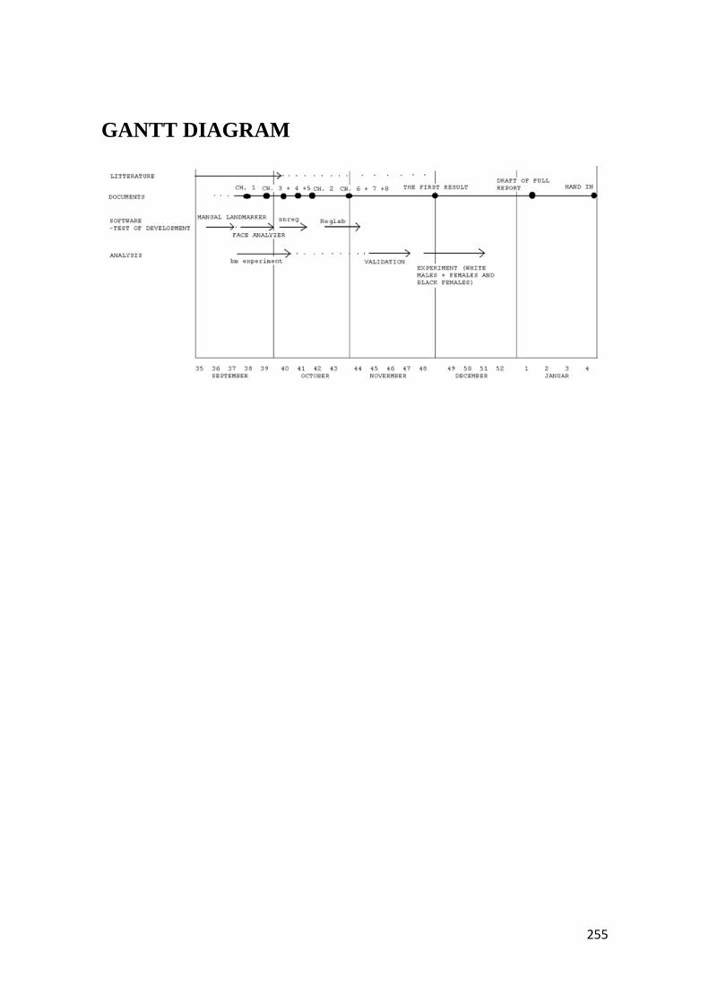
255
GANTT DIAGRAM

Appendix E.2
256
Appendix E.2
Learning objectives
Learning objectives for my Master’s project consists of objectives related to the
”generic” learning objectives stated by DTU, as well as to specific learning objectives of
my particular project.
Generic Learning Objectives
At the end of the Master’s project period, I should have demonstrated that I am able
to:
Understand problems which forms a part of the technology used in the thesis.
Comprehend problems in the thesis and on the basis of that set up different
options.
Develop new ideas and solve problems.
Formulate, communicate and write in Danish and English.
Analyze, discuss and conclude on new results.
Handle unexpected problems.
Learn and use different tools.
Specific Learning Objectives
At the end of the Master’s project period, I should be able to:
Define and discuss the concept of facial asymmetry
Design, implement and apply software programs for analysis of 3D point data
and polygonal surface models

257
Define and discuss the following key concepts in shape analysis /
morphometrics:
- Transformation matrices; rigid and non-rigid image
registration; detailed point correspondence.
Define and discuss the concepts of mean and variability in a group
Apply principal components analysis to a dataset consisting of a number of 3D
shapes