Quality vs. Variety: Trading Larger Screens for More

Shows in the Era of Digital Cinema

Anita Rao Wesley R. Hartmann

Booth School of Business Graduate School of Business

University of Chicago Stanford University

January 27 2015

Abstract

Movie exhibitors currently face two forces vying for the limited footprint of their

properties. Recent advances have enabled exhibitors to satisfy consumers’ long-standing

desire for increasingly larger screens. On the other hand, digital technology has reduced

the cost of playing the same movie on multiple screens, thereby creating an incentive

for screen proliferation to increase the number of show times for a given movie. In-

creasing the screens also has the added benefit of allowing the exhibitor to expand the

number of unique movies screened at a given time. This is fundamentally a tradeoff

between quality (larger screen size) and variety (more movies or showings). The goal

of this paper is to evaluate consumers’ relative valuations of the large screens vs. more

shows tradeoff. We use a new data set on movie showings in India at the movie-chain-

market-week level to estimate an aggregate discrete-choice demand model providing

measures of customer preferences for the number of movie showings and screen size.

India provides a valuable setting to study this question because the densely populated

cities face substantial space constraints and regional heterogeneity in tastes and lan-

guages suggest the option of more shows may be more important in some cities than

others. Our findings suggest that regions which are more urban and have a greater

share of people with higher education prefer larger screens (quality) while most other

regions prefer more showings (variety).

1

1 Introduction

Providing the variety of products necessary to meet diverse customers’ needs often entails

sacrifices in quality. For example, Netflix and other movie subscription services aiming to

provide a large selection of movies have trouble providing new blockbusters or classics in

their lineup. A similar tradeoff between variety and quality arises in movie exhibition. New

digital technology enables the same movie to be shown across multiple screens at overlap-

ping times. The quality tradeoff in this case is that exhibitors are considering shrinking

screen/auditorium sizes to expand the number of screens and hence potential show times.

We consider how consumers tradeoff variety vs. quality in this case of movies where the

number of screens vs. the size of each involves a relatively simple tradeoff in how square

footage is allocated.

An anecdote from the earliest days of cinema is “the bigger the image, the greater the

impact on the viewer”.1 Nevertheless, exhibitors have been shrinking screen sizes as they try

to offer a greater variety of movies or greater time flexibility in when a movie is shown. We

consider movie exhibitors production of multiplexes in India where recent economic growth

is fueling a push toward new theater construction and use of digital technology. The Indian

market is insightful to study for three main reasons. First, entrants of new theaters are space

constrained by the densely populated cities and therefore cannot afford to build many large

screens within a multiplex. Second, there is substantial regional heterogeneity in the breadth

of movies watched by the local population suggesting variable preferences for variety. Finally,

India is unique in empirically analyzing screen size because customers there are well-versed

with the screen size a movie will play in before buying the tickets. Exhibitors often list the

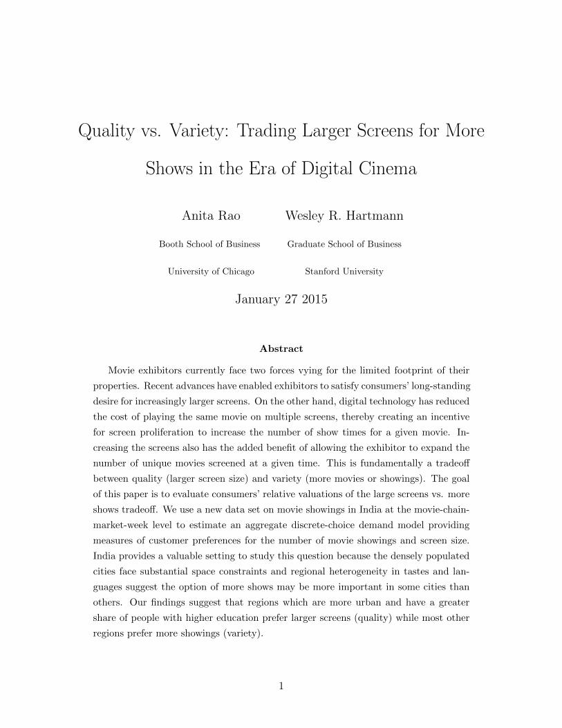
screens in which movies will play (see Figure 1 for the choices that come up before a consumer

finalizes her theater booking. The movie Terminator Salvation is available in two auditoria -

Sathyam and Seasons.) This allows our identification to exploit screen size differences within

a theater in addition to the more salient screen size differences across theaters.

1Quoted from http://www.imax.com.au/visitor info/

2

Figure 1: A consumer can choose both the screen and showtime before booking the movie

Our dataset consists of the number of admits, revenues and number of showings for

movies screened between March 2007 and February 2008 at the chain-market-week level. We

supplement this data with seat-layout charts, across all theaters in our dataset, which allows

us to infer the screen width of each auditorium within a chain. We also use demographic

data from the 2001 Census to account for regional heterogeneity.

To analyze the data and evaluate the quality vs. variety tradeoff, we use a demand model

similar to that of Davis (2006), who considers whether theater scale choices are optimal.

A fundamental difference between our approaches is that he treats the number of screens

in a “descriptive” sense by assuming they enter the consumer’s utility directly. However,

we believe that a consumer’s utility is driven by the variety screens can create in terms

of the diversity of movies that can be shown or the number of showings of a given movie.

Specifically, in regions where customers demand a greater variety of movies, or more showings

for a given movie, additional screens will deliver more value than other areas. Furthermore,

we compare the value of screens in terms of variety against an explicit opportunity cost: the

increase in screen sizes that could have been achieved in place of the extra screen.

Our results indicate that the impact of adding one more show is higher than the impact

of increasing screen size. This justifies to some extent the recent shift to multiplexes in India.

However, we show that the extent of this impact is market-specific. We find that markets

which are more urban and have a higher percentage of people with higher education prefer

3

larger screens.

The empirical literature studying product quality and variety has largely addressed this

from the perspective of competition and differentiation (e.g. Draganska, Mazzeo and Seim

2008; Orhun et al 2014; Mazzeo 2003), with little emphasis on consumers’ taste for quality

and variety. Perhaps closest to our idea of the quality-variety tradeoff is Bohlmann, Golder

and Mitra (2002) who theoretically show that pioneers are likely to succeed in markets where

consumers’ taste for variety is higher than the taste for quality. Our paper contributes to this

literature by measuring consumers’ preference for quality and variety in a setting where a

firm providing one has to necessarily sacrifice the other2. Aside from the variety vs. quality

tradeoffs, our findings contribute to a growing empirical literature on the movie industry

that has covered topics ranging from organizational issues such as movie financing decisions

(e.g. Goettler and Leslie, 2005) and contracting (e.g. Gil, 2013) to operational issues such

as release and run-length (e.g. Einav, 2007 and Ainslie, Dreze and Zufryden, 2005), pricing

(Gil and Hartmann, 2009), and finally post-box office distribution (Mortimer, 2007 and

Mortimer 2008). Our analyses is also an input to the determination of the “shelf space” to be

allocated in theaters as described by Elberse and Eliashberg (2003). To date this literature

has primarily focused on allocating products within this space (e.g. Eliashberg et.al. 2006).

The rest of the paper is organized as follows. The next section outlines the data. Section

3 defines the empirical model and identification. Section 4 provides the model estimates and

Section 5 concludes.

2 Data

We use a data set on movie showings in India at the movie-chain-market-week level. Variation

in screen size as well as number of shows, necessary to answer our question, is present in

our data set. The dataset consists of admits, net collections, shows, occupancy and spans 14

markets, 7 chains, 44 weeks (March 2007 – February 2008) and nearly 600 unique movies.

2This ignores costs associated with provision of higher quality and higher variety.

4

The number of screens specific to a chain in a market was obtained from the chain website.

While each chain has only one multiplex in a market, the number of competing chains in

each market ranges from two to four.

Unlike the US, prices of showings in India vary across markets, chains, movies and time.

Weekly price of each movie showing in a chain-market was calculated by dividing the net

collections by the total admits.

The number of showings and the occupancy percentage for each movie-chain-market-week

combination are available directly from the data. Using the occupancy and admits data, we

infer the total seating capacity for each movie showing as:

seatsjclt =admitsjclt

occupancyjclt × showsjclt(1)

Here j indexes movies, c theater-chains, l locations and t the week of the showing.

To map the number of seats to an auditorium’s screen width we collect a secondary source

of data on each chain’s seating configuration for 30 out of the 34 chain-location combinations

from the website http://in.bookmyshow.com (the remaining 4 chains are no longer active

in the market). in.bookmyshow.com is an online ticket booking portal where consumers

can search for movies by chain, location, date and showing. Upon clicking on a particular

showing, they are directed to a seat-layout chart and prompted to select their seats and

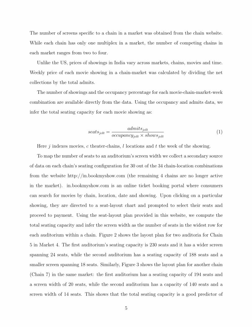
proceed to payment. Using the seat-layout plan provided in this website, we compute the

total seating capacity and infer the screen width as the number of seats in the widest row for

each auditorium within a chain. Figure 2 shows the layout plan for two auditoria for Chain

5 in Market 4. The first auditorium’s seating capacity is 230 seats and it has a wider screen

spanning 24 seats, while the second auditorium has a seating capacity of 188 seats and a

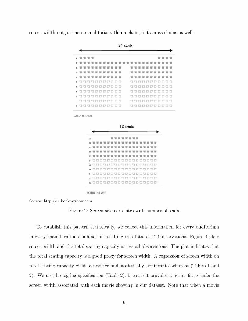
smaller screen spanning 18 seats. Similarly, Figure 3 shows the layout plan for another chain

(Chain 7) in the same market: the first auditorium has a seating capacity of 194 seats and

a screen width of 20 seats, while the second auditorium has a capacity of 140 seats and a

screen width of 14 seats. This shows that the total seating capacity is a good predictor of

5

screen width not just across auditoria within a chain, but across chains as well.

Source: http://in.bookmyshow.com

Figure 2: Screen size correlates with number of seats

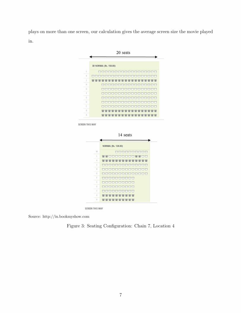
To establish this pattern statistically, we collect this information for every auditorium

in every chain-location combination resulting in a total of 122 observations. Figure 4 plots

screen width and the total seating capacity across all observations. The plot indicates that

the total seating capacity is a good proxy for screen width. A regression of screen width on

total seating capacity yields a positive and statistically significant coefficient (Tables 1 and

2). We use the log-log specification (Table 2), because it provides a better fit, to infer the

screen width associated with each movie showing in our dataset. Note that when a movie

6

plays on more than one screen, our calculation gives the average screen size the movie played

in.

Source: http://in.bookmyshow.com

Figure 3: Seating Configuration: Chain 7, Location 4

7

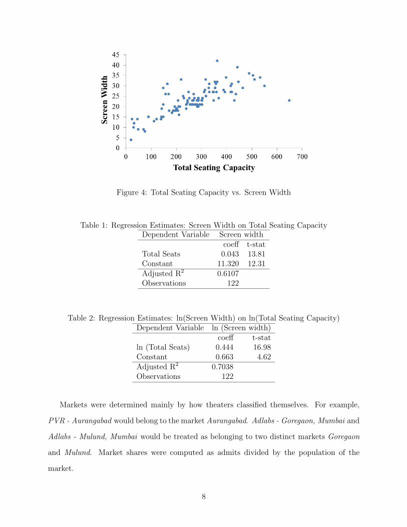
Figure 4: Total Seating Capacity vs. Screen Width

Table 1: Regression Estimates: Screen Width on Total Seating CapacityDependent Variable Screen width

coeff t-statTotal Seats 0.043 13.81Constant 11.320 12.31Adjusted R2 0.6107Observations 122

Table 2: Regression Estimates: ln(Screen Width) on ln(Total Seating Capacity)Dependent Variable ln (Screen width)

coeff t-statln (Total Seats) 0.444 16.98Constant 0.663 4.62Adjusted R2 0.7038Observations 122

Markets were determined mainly by how theaters classified themselves. For example,

PVR - Aurangabad would belong to the market Aurangabad. Adlabs - Goregaon, Mumbai and

Adlabs - Mulund, Mumbai would be treated as belonging to two distinct markets Goregaon

and Mulund. Market shares were computed as admits divided by the population of the

market.

8

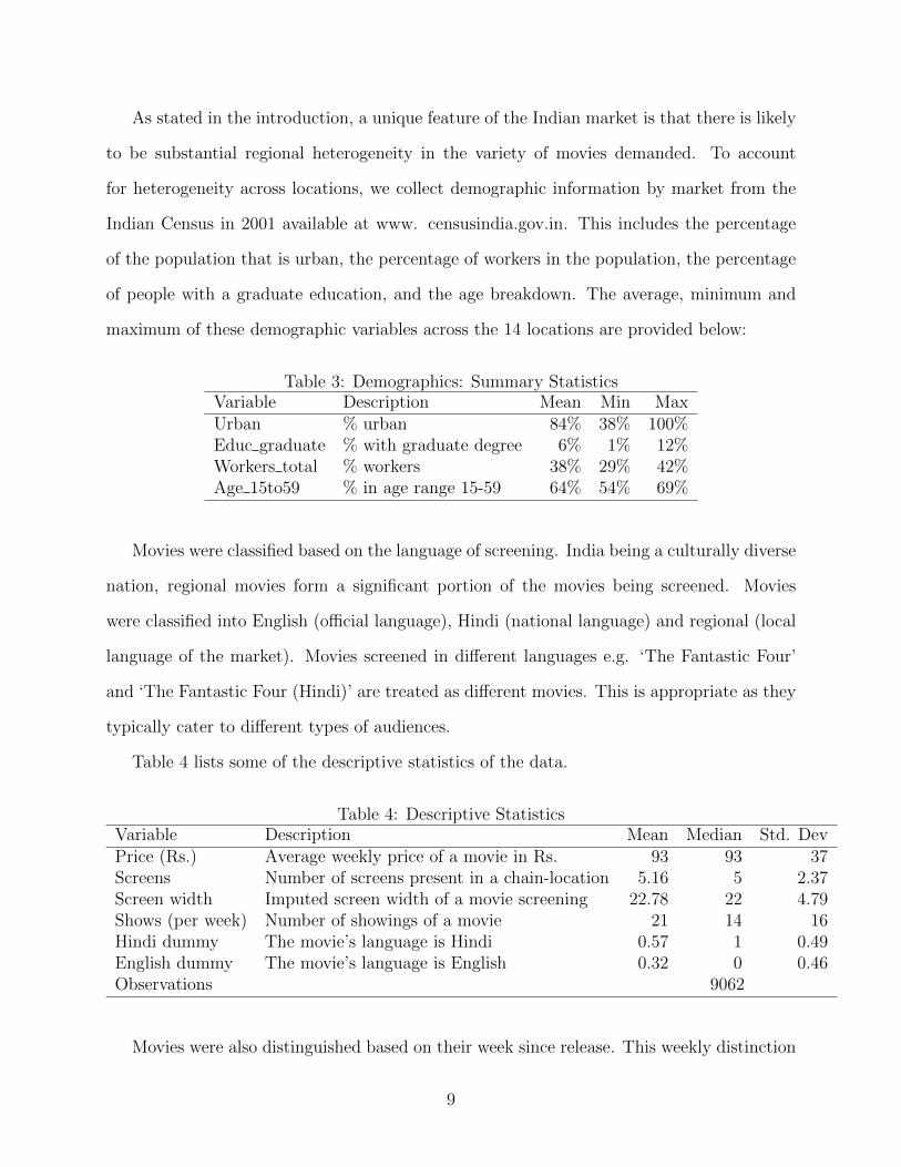
As stated in the introduction, a unique feature of the Indian market is that there is likely

to be substantial regional heterogeneity in the variety of movies demanded. To account

for heterogeneity across locations, we collect demographic information by market from the

Indian Census in 2001 available at www. censusindia.gov.in. This includes the percentage

of the population that is urban, the percentage of workers in the population, the percentage

of people with a graduate education, and the age breakdown. The average, minimum and

maximum of these demographic variables across the 14 locations are provided below:

Table 3: Demographics: Summary StatisticsVariable Description Mean Min MaxUrban % urban 84% 38% 100%Educ graduate % with graduate degree 6% 1% 12%Workers total % workers 38% 29% 42%Age 15to59 % in age range 15-59 64% 54% 69%

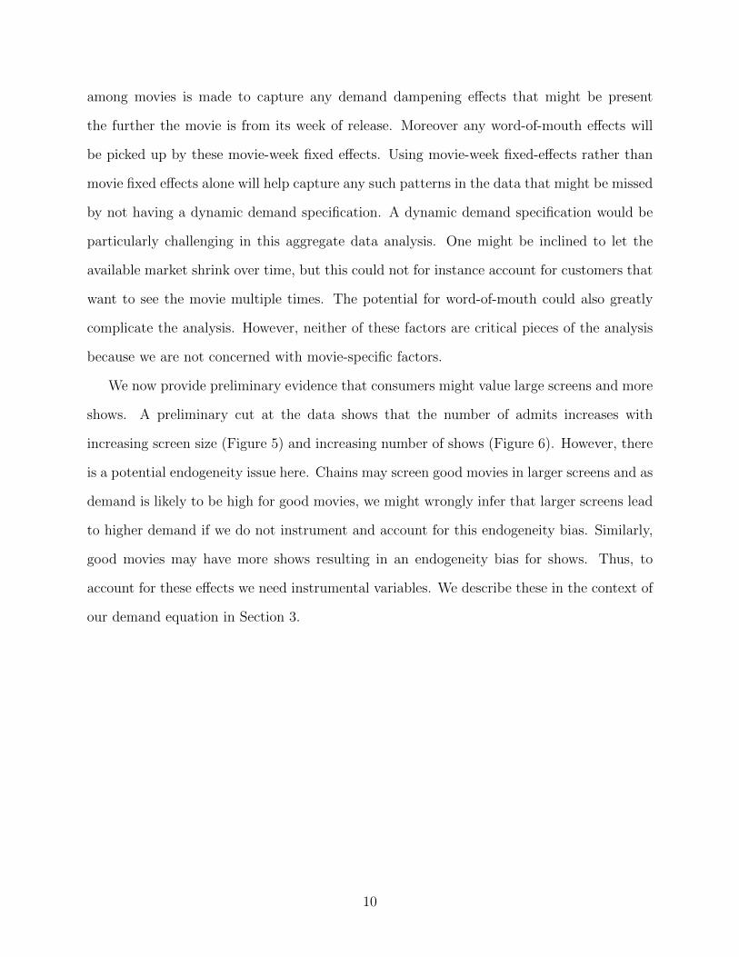
Movies were classified based on the language of screening. India being a culturally diverse

nation, regional movies form a significant portion of the movies being screened. Movies

were classified into English (official language), Hindi (national language) and regional (local

language of the market). Movies screened in different languages e.g. ‘The Fantastic Four’

and ‘The Fantastic Four (Hindi)’ are treated as different movies. This is appropriate as they

typically cater to different types of audiences.

Table 4 lists some of the descriptive statistics of the data.

Table 4: Descriptive StatisticsVariable Description Mean Median Std. DevPrice (Rs.) Average weekly price of a movie in Rs. 93 93 37Screens Number of screens present in a chain-location 5.16 5 2.37Screen width Imputed screen width of a movie screening 22.78 22 4.79Shows (per week) Number of showings of a movie 21 14 16Hindi dummy The movie’s language is Hindi 0.57 1 0.49English dummy The movie’s language is English 0.32 0 0.46Observations 9062

Movies were also distinguished based on their week since release. This weekly distinction

9

among movies is made to capture any demand dampening effects that might be present

the further the movie is from its week of release. Moreover any word-of-mouth effects will

be picked up by these movie-week fixed effects. Using movie-week fixed-effects rather than

movie fixed effects alone will help capture any such patterns in the data that might be missed

by not having a dynamic demand specification. A dynamic demand specification would be

particularly challenging in this aggregate data analysis. One might be inclined to let the

available market shrink over time, but this could not for instance account for customers that

want to see the movie multiple times. The potential for word-of-mouth could also greatly

complicate the analysis. However, neither of these factors are critical pieces of the analysis

because we are not concerned with movie-specific factors.

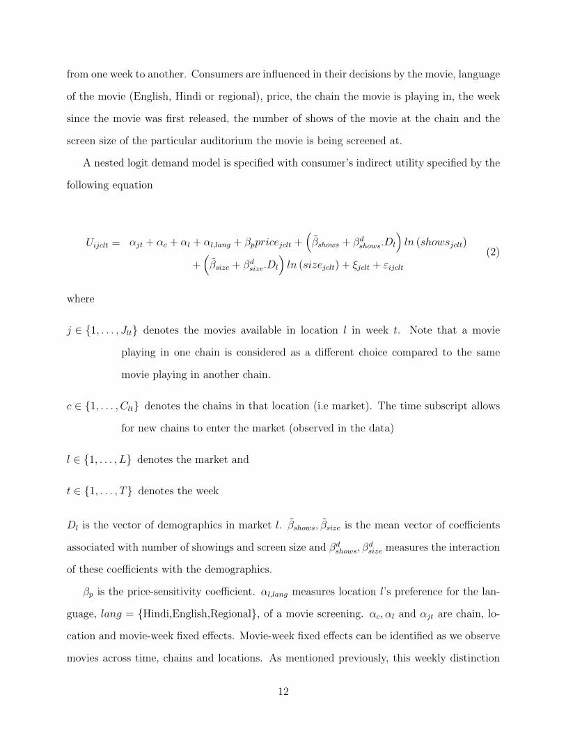
We now provide preliminary evidence that consumers might value large screens and more

shows. A preliminary cut at the data shows that the number of admits increases with

increasing screen size (Figure 5) and increasing number of shows (Figure 6). However, there

is a potential endogeneity issue here. Chains may screen good movies in larger screens and as

demand is likely to be high for good movies, we might wrongly infer that larger screens lead

to higher demand if we do not instrument and account for this endogeneity bias. Similarly,

good movies may have more shows resulting in an endogeneity bias for shows. Thus, to

account for these effects we need instrumental variables. We describe these in the context of

our demand equation in Section 3.

10

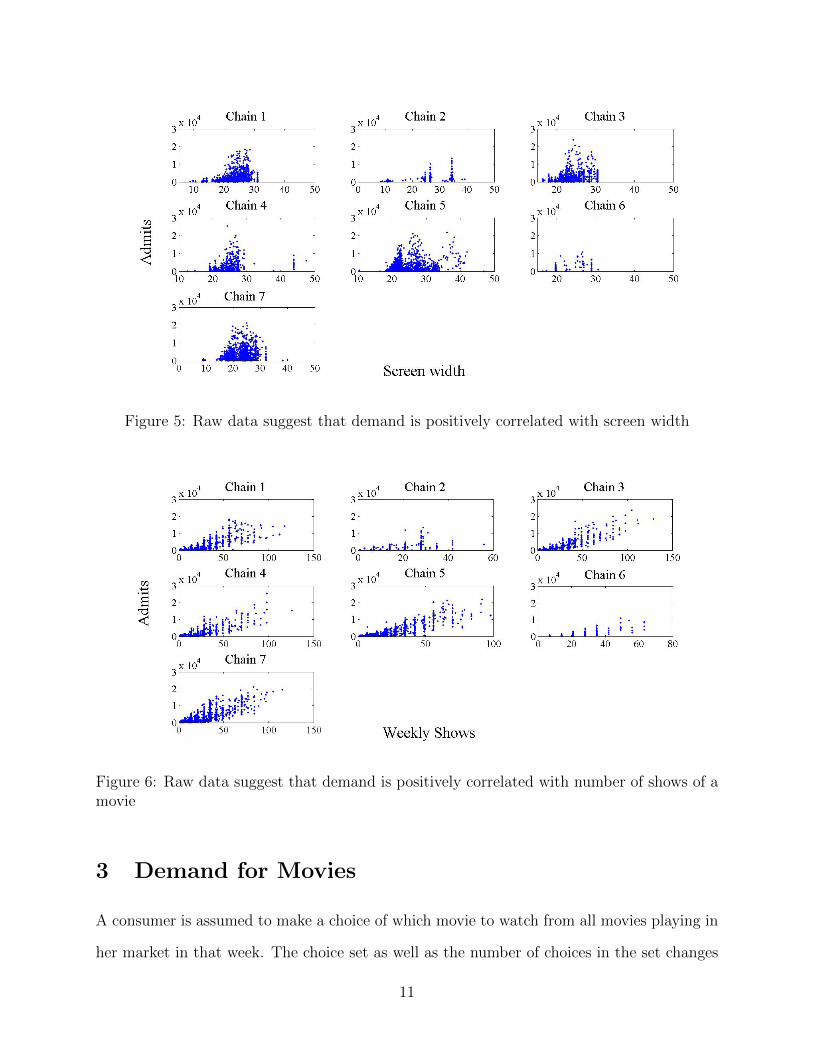
Figure 5: Raw data suggest that demand is positively correlated with screen width

Figure 6: Raw data suggest that demand is positively correlated with number of shows of amovie

3 Demand for Movies

A consumer is assumed to make a choice of which movie to watch from all movies playing in

her market in that week. The choice set as well as the number of choices in the set changes

11

from one week to another. Consumers are influenced in their decisions by the movie, language

of the movie (English, Hindi or regional), price, the chain the movie is playing in, the week

since the movie was first released, the number of shows of the movie at the chain and the

screen size of the particular auditorium the movie is being screened at.

A nested logit demand model is specified with consumer’s indirect utility specified by the

following equation

Uijclt = αjt + αc + αl + αl,lang + βppricejclt +(β̃shows + βdshows.Dl

)ln (showsjclt)

+(β̃size + βdsize.Dl

)ln (sizejclt) + ξjclt + εijclt

(2)

where

j ∈ {1, . . . , Jlt} denotes the movies available in location l in week t. Note that a movie

playing in one chain is considered as a different choice compared to the same

movie playing in another chain.

c ∈ {1, . . . , Clt} denotes the chains in that location (i.e market). The time subscript allows

for new chains to enter the market (observed in the data)

l ∈ {1, . . . , L} denotes the market and

t ∈ {1, . . . , T} denotes the week

Dl is the vector of demographics in market l. β̃shows, β̃size is the mean vector of coefficients

associated with number of showings and screen size and βdshows, βdsize measures the interaction

of these coefficients with the demographics.

βp is the price-sensitivity coefficient. αl,lang measures location l’s preference for the lan-

guage, lang = {Hindi,English,Regional}, of a movie screening. αc, αl and αjt are chain, lo-

cation and movie-week fixed effects. Movie-week fixed effects can be identified as we observe

movies across time, chains and locations. As mentioned previously, this weekly distinction

12

among movies is made to help tease out any patterns in the data that might be missed by not

having a dynamic demand specification (e.g. demand dampening, word-of mouth effects).

ξjclt is the unobserved (to the researcher) characteristic, e.g. the location-specific quality of

a movie in a given week, and εijclt is the unobserved individual-specific demand shock.

The choices are partitioned into 2 groups with group 1 consisting of the set of all movies

playing in that location that week and group 2 consisting of the outside alternative (see

Figure 7).

Figure 7: Nested Logit Specification

Following the nested logit formulation, we assume the joint distribution of ε in each

market-week as

F (ε0, ε1, ε2, . . . , εJlt) = exp

(−exp (−ε0)−

[Jlt∑j=1

exp(−ρ−1εj

)]ρ)(3)

The share equation for each movie-chain-market-week is then given by

sjclt =exp

(Vjcltρ

)( ∑k∈Jlt

exp(Vkcltρ

))1−ρ(1 +

( ∑k∈Jlt

exp(Vkcltρ

))ρ)where Vjclt = Uijclt − εijclt.

After a few transformations, this translates into the following system of equations

13

ln (sjclt)− ln (s0lt) = αjt + αc + αl + αl,lang + βppricejclt + βshowsln (showsjclt) + βsizeln (seatsjclt)

+ξjclt + (1− ρ) ln(

sjclt1−s0lt

)(4)

The standard logit model is obtained when the nesting parameter ρ is 1. When the

nesting parameter is 0 there is no substitution between the outside option and the movies

nest.

3.1 Endogeneity

Endogeneity can bias the estimates of seats and shows, the main variables of interest, if not

accounted for appropriately. Good movies will have more shows and may also be screened in

larger screens; these movies will also have high demand. This endogeneity would lead to an

upward bias in the estimate for shows and screen size effects. The movie-time fixed effects,

αjt, reduce concerns about this bias, but there still could be some local demand shocks for the

movies which are correlated with the theater’s choice of how many showings or how large a

screen to assign. Econometrically, this implies a correlation between ξjclt and the variables of

interest (shows and screen size) chosen at the jclt level. We remove this systematic variation

by shifting inference, within movie and time, to cross-chain variation in shows and screen

size that is based only on the predetermined chain-location dimensions (number of screens

and screen sizes). In other words, by using the predetermined chain-location dimensions as

instruments, we remove the variation that is tied directly to how a given movie is matched

with the particular number or size of screens in the chain and location.3

We instrument for the number showings with the number of available screens at the chain-

location. The total number of screens is a good instrument because 1. It is pre-determined

3One critique of this approach is that the predicted number of showings is the same for all movieswithin a chain-location, such that a fixed effect at the chain-location level would remove all variation inthis instrument. In the presence of such a fixed effect, an interaction between the instrument and moviecharacteristics indexed by jt would remove such a concern and predict different numbers of showings acrossmovies within a chain-location.

14

i.e., theaters cannot adjust the total number of screens in response to demand shocks and

2. It is correlated with the number of shows of a movie at a theater, i.e. a chain with

more screens can have more showings. We instrument for the screen size using a summary

statistic of the various screen sizes available at the chain-location. Specifically, we use an

HHI described in Equation 5 below, that distinguishes between the kinds of screen width

present in a given chain. This instrument distinguishes, for example between two theaters

with the same total screen width of 50 seat-wide screens, one with one 40-seat wide screen

and one 10-seat wide screen and another with two 25-seat wide screens. It removes the

endogeneity concerns in much the same way as the number of screens instruments, because

it shifts the potential screen size. Both of these instruments are clearly correlated with the

observed showings/screen sizes, yet are uncorrelated with the characteristics of any given

movie because they were determined well before the observed movies were ever produced.

hhic =Nc∑i=1

(screen widthi∑i screen widthi

)2

(5)

where i refers to an auditorium in chain c which has a total of N auditoria.

Apart from accounting for endogeneity biases in seats and shows, we also have to account

for endogeneity that arises from the nesting parameter in Equation 4. A good instrument is

one that is unrelated to the share of the movie relative to the outside good but is correlated

with the share within the movie nest. Valid instruments include the total number of Hindi

(and English) movies playing in that market-week other than the movie under considera-

tion. Einav (2007) uses the total number of movies playing other than the movie under

consideration as an instrument and argues that including week- and movie- fixed effects will

remove any endogeneity associated with the fact that more movies may be associated with

high-demand weeks and that fewer movies may be released along with a high-quality movie

respectively. We use all three instruments discussed above to account for endogeneity of the

nesting parameter.

Lastly, we instrument for price using the average price of other movies being screened in

15

the particular chain that week.

3.2 Estimation

The estimation recovers β∗, the true parameter vector, that satisfies

E [ξ (β∗)Z] = 0

This translates to minimizing the GMM objective function

ξ (β)′ZΦ−1Z

′ξ (β)

where Z is the vector of instruments discussed above. ξ (β) = Y − Xβ where Y =

ln (sjclt)−ln (solt) andXβ is the RHS of Equation 4. Φ is a consistent estimate of E[Z

′ww

′Z].

4 Results

Table 5 presents the estimates of the model before4 and after accounting for the endogeneity

bias. As can be seen by the reduction in the magnitude of the shows and seats coefficients,

the direction of the endogeneity correction is in line with the potential biases we described

above. The coefficients for price, shows and seats coefficients have the intuitive sign and

are statistically significant. Chain, market and movie-week fixed effects are included in all

specifications.

Specification S1 illustrates the baseline correlation between admits and the variables of

interest: shows and screen size. The positive and significant coefficients reaffirm the patterns

described in Figures 5 and 6 even after controlling for the price, language of the movie, and

chain, location and movie-week effects. Next, in S2, we evaluate whether these relationships

4We do not include the nesting parameter in the before estimation as without instrumenting for the nest,this parameter - which is highly correlated with the dependant variable - explains most of the variation inthe data.

16

vary across markets based on demographics. Clearly demographic variables seem to be

important. Specification S3 accounts for both the endogeneity in these variables and the

potential correlations among options in the choice set via a nested logit. One noticeable

change between S3 and S2 is that the sign of the demographic interactions with the shows

coefficient reverses. This likely reflects that S2 was picking up correlations between the

demands of these demographic groups and the showings. For example, more shows may have

been allocated where workers are less likely to go to the movies, but once the endogeneity

is accounted for, markets with more workers tend to prefer more showings, all else equal.

We also estimated a random coefficients model (Berry, Levinsohn and Pakes 1995, Nevo

2000) that allows for more flexible substitution patterns. However, the estimates of the

unobserved heterogeneity were insignificant, leading us to conclude that the nested-logit

specification with movie-week fixed-effects is picking up most of the variation in the data.

Finally S4 restricts the shows and screen-size coefficients to be positive. The transformation

we use for these two variables is:

β = eβ̃+βd(Dl)

where Dl is the vector of demographics in market l, β̃ is the mean vector of coefficients

βshows, βscreenwidth and βd measures the interaction of these coefficients with the demographics.

This transformation is done to avoid negative estimates of the screen and shows coefficients

at some extreme values of the demographics which arises due to the linear specification.

Across both specifications S3 and S4, the estimates indicate that more urban areas and

markets with a larger share of consumers with higher education prefer wider screens (qual-

ity) while markets with a greater share of total workers prefer more shows (variety). The

estimates also indicate a nesting parameter significantly different from 1 suggesting that the

nested logit model fits the data better than the standard logit model. Appendix A presents

the first-stage regression results (for S3) showing the validity of the instruments.

17

Table 5: Estimates across various specificationsS1 S2 S3 S4

Instruments No No Yes YesNest No No Yes Yesln(Shows) 0.992 1.605 -8.183 -10.350

(84.19) (9.75) (-7.01) (-2.97)

ln(Shows) X Urban -0.180 1.759 2.742(-4.28) (3.99) (3.32)

ln(Shows) X Educ graduate -1.350 6.146 8.741(-6.81) (2.83) (3.55)

ln(Shows) X Workers total -0.999 17.434 17.434(-2.85) (6.38) (2.06)

ln(Screen width) 0.767 -5.963 -6.232 -7.972(23.30) (-7.51) (-2.22) (-2.69)

ln(Screen width) X Urban 1.198 3.060 3.931(5.72) (4.15) (2.33)

ln(Screen width) X Educ graduate 10.939 12.386 10.750(10.91) (3.07) (2.91)

ln(Screen width) X Workers total 13.268 9.021 8.553(8.01) (1.58) (1.69)

Price -0.0003 0.001 -0.002 -0.003(-1.23) (2.57) (-3.48) (-5.55)

Nesting Parameter, rho 0.181 0.256(5.50) (10.53)

Fixed-Effects: Chain, Market, Market-Language, Movie-WeekAdjusted R2 0.9344 0.9354 0.9607 N/AGMM Objective Function 13.5811 16.091

Figure 8 plots the change in willingness to pay , if one more show were added (More

shows) or the screen size was widened by an equivalent of five seats (Larger screen). The

1 to 5 ratio reflects the opportunity cost of shows in terms of screen size or vice versa

and is derived based on an auditorium being able to provide 5 additional show times and

18

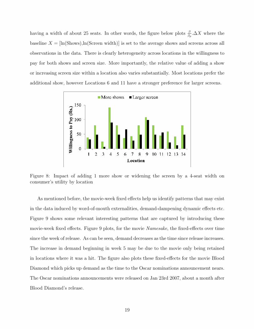
having a width of about 25 seats. In other words, the figure below plots ββp.∆X where the

baseline X = [ln(Shows),ln(Screen width)] is set to the average shows and screens across all

observations in the data. There is clearly heterogeneity across locations in the willingness to

pay for both shows and screen size. More importantly, the relative value of adding a show

or increasing screen size within a location also varies substantially. Most locations prefer the

additional show, however Locations 6 and 11 have a stronger preference for larger screens.

Figure 8: Impact of adding 1 more show or widening the screen by a 4-seat width onconsumer’s utility by location

As mentioned before, the movie-week fixed effects help us identify patterns that may exist

in the data induced by word-of-mouth externalities, demand-dampening dynamic effects etc.

Figure 9 shows some relevant interesting patterns that are captured by introducing these

movie-week fixed effects. Figure 9 plots, for the movie Namesake, the fixed-effects over time

since the week of release. As can be seen, demand decreases as the time since release increases.

The increase in demand beginning in week 5 may be due to the movie only being retained

in locations where it was a hit. The figure also plots these fixed-effects for the movie Blood

Diamond which picks up demand as the time to the Oscar nominations announcement nears.

The Oscar nominations announcements were released on Jan 23rd 2007, about a month after

Blood Diamond’s release.

19

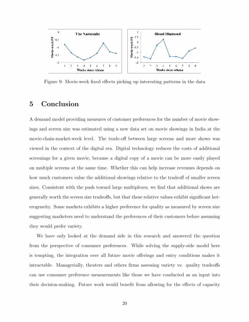
Figure 9: Movie-week fixed effects picking up interesting patterns in the data

5 Conclusion

A demand model providing measures of customer preferences for the number of movie show-

ings and screen size was estimated using a new data set on movie showings in India at the

movie-chain-market-week level. The trade-off between large screens and more shows was

viewed in the context of the digital era. Digital technology reduces the costs of additional

screenings for a given movie, because a digital copy of a movie can be more easily played

on multiple screens at the same time. Whether this can help increase revenues depends on

how much customers value the additional showings relative to the tradeoff of smaller screen

sizes. Consistent with the push toward large multiplexes, we find that additional shows are

generally worth the screen size tradeoffs, but that these relative values exhibit significant het-

erogeneity. Some markets exhibits a higher preference for quality as measured by screen size

suggesting marketers need to understand the preferences of their customers before assuming

they would prefer variety.

We have only looked at the demand side in this research and answered the question

from the perspective of consumer preferences. While solving the supply-side model here

is tempting, the integration over all future movie offerings and entry conditions makes it

intractable. Managerially, theaters and others firms assessing variety vs. quality tradeoffs

can use consumer preference measurements like those we have conducted as an input into

their decision-making. Future work would benefit from allowing for the effects of capacity

20

constraints and the associated spillovers between movies.

References

[1] Ainslie, A., D. Xavier and F.Zufryden (2005), “Modeling Movie Life Cycles and

Market Share”, Marketing Science, 24(3), 508-517

[2] Berry, S., J. Levinsohn and A. Pakes (1995), “Automobile Prices in Market

Equilibrium,” Econometrica, 63, 841–890

[3] Bohlmann, J.D., P. N. Golder and D. Mitra (2002), “Deconstructing the Pi-

oneer’s Advantage: Examining Vintage Effects and Consumer Valuations of

Quality and Variety”, Management Science 48(9), 1175-1195

[4] Davis, P. (2006), “Spatial Competition in Retail markets: Movie Theaters,”

RAND Journal of Economics, 37(4), 964-982

[5] Draganska, M., M. Mazzeo and K. Seim (2009), “Beyond Plain Vanilla: Mod-

eling Joint Pricing and Product Assortment Choices”, Quantitative Marketing

and Economics, 7(2), 105-146

[6] Einav, L. (2007), “Seasonality in the U.S. Motion Picture Industry”, RAND

Journal of Economics, 38(1), 127-145

[7] Elberse, A. and J. Eliashberg (2003), “Demand and supply dynamics for sequen-

tially released products in international markets: The case of motion pictures”,

Marketing Science, 22(3), 329-354

[8] Eliashberg, J., A. Elberse and M. Leenders (2006), “The Motion Picture In-

dustry: Critical Issues in Practice, Current Research, and New Research Direc-

tions”, Marketing Science, 25(6), 638-661

21

[9] Gil, R. (2013), “The Interplay of Formal and Relational Contracts: Evidence

from Movies”, The Journal of Law, Economics and Organization, 29(3), 681-710

[10] Gil, R. and W.R. Hartmann (2009), “Empirical Analysis of Metering Price

Discrimination: Evidence from Concession Sales at Movie Theaters”, Marketing

Science, 28(6), 1046-1062

[11] Goettler, R.L. and P. Leslie (2005), “Cofinancing to Manage Risk in the Motion

Picture Industry”, Journal of Economics and Management Strategy, 14(2), 231-

26

[12] Mazzeo, M. (2003), “Competition and Service Quality in the U.S. Airline In-

dustry”, Review of Industrial Organization, 22(4), 275-296

[13] Mortimer, J. (2007), “Price Discrimiation, Copyright Law, and Technological

Innovation: Evidence from the introduction of DVDs”, The Quarterly Journal

of Economics, 122 (3), 1307-1350

[14] Mortimer, J. (2008), “Vertical Contracts in the Video Rental Industry”, The

Review of Economic Studies, 75 (1), 165-199

[15] Nevo, A. (2000), “A Practitioner’s Guide to Estimation of Random-Coef cients

Logit Models of Demand”, Journal of Economics & Management Strategy, 9(4),

513-548

[16] Orhun, Y., P. Chintagunta and S. Venkataraman (2014), Impact of Competition

on Product Decisions: Movie Choices of Exhibitors, working paper, Ross School

of Business.

[17] Train, K. (2003), Discrete Choice Methods with Simulation, Cambridge Uni-

versity Press

22

A First-Stage Regression

Table 6 presents the first-stage regression results for the main variables of interest - price,

ln(Shows), ln(Screen Width) and the nesting parameter - specific to Specification S3. The

number of screens in a chain was the instrument for shows. The significant coefficients on

screensXhhi indicates that screens and shows are correlated. The overall effect at the average

demographic is positive indicating that a chain with more screens (and a higher hhi) has more

shows. The instrument for screen size - hhi - is such that it takes on large values when a

chain has more variation in screen sizes across its auditoria and also when there are more

screens. The overall coefficient on hhi and hhi2 at the average demographic is significantly

negative, indicating that such chains are more likely to screen movies in auditoria with

smaller screens. The instrument for the nesting parameter - 1/(No. competing movies) -

takes on larger values when there are fewer competing movies playing in the market. A

positive coefficient indicates that the inside-nest share of the movie is higher when there are

fewer competing movies playing. The average price of other movies playing in a chain that

week is positively correlated with the price of the focal movie.

23

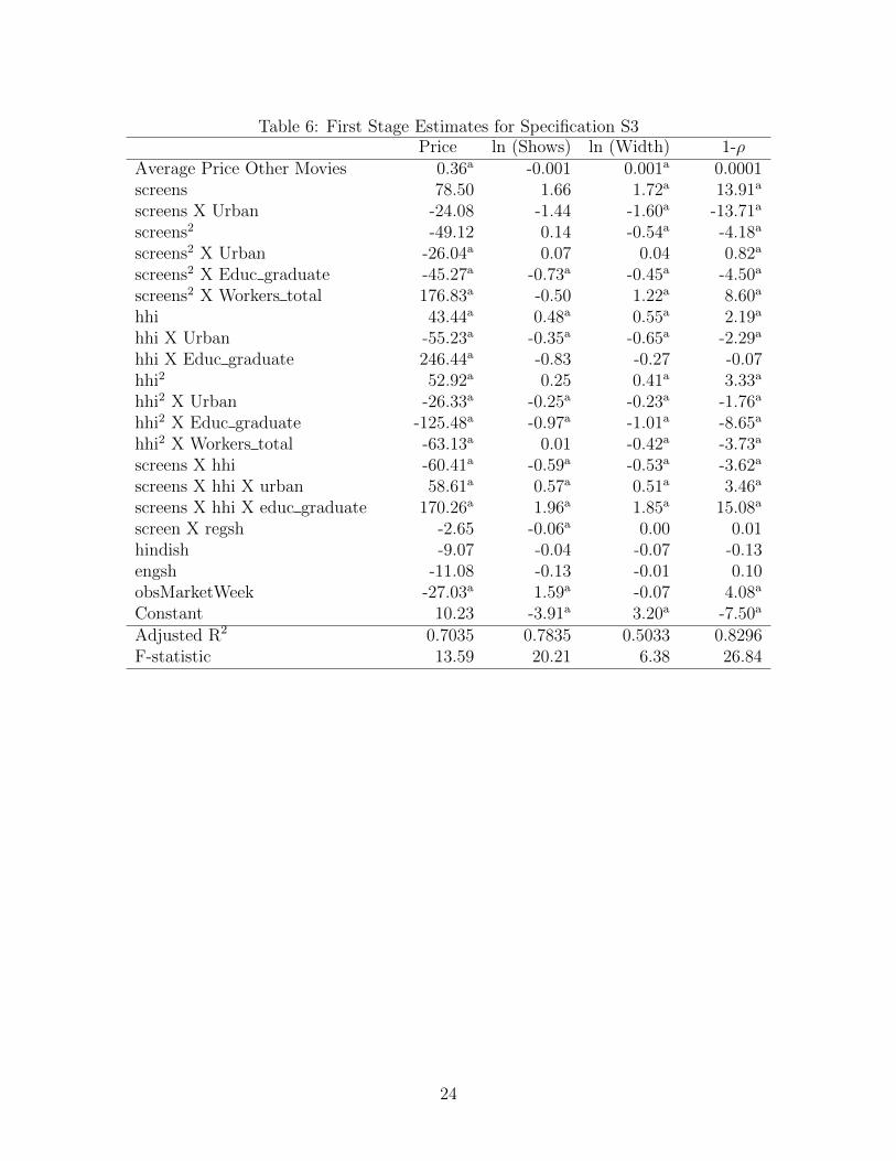
Table 6: First Stage Estimates for Specification S3Price ln (Shows) ln (Width) 1-ρ

Average Price Other Movies 0.36a -0.001 0.001a 0.0001screens 78.50 1.66 1.72a 13.91a

screens X Urban -24.08 -1.44 -1.60a -13.71a

screens2 -49.12 0.14 -0.54a -4.18a

screens2 X Urban -26.04a 0.07 0.04 0.82a

screens2 X Educ graduate -45.27a -0.73a -0.45a -4.50a

screens2 X Workers total 176.83a -0.50 1.22a 8.60a

hhi 43.44a 0.48a 0.55a 2.19a

hhi X Urban -55.23a -0.35a -0.65a -2.29a

hhi X Educ graduate 246.44a -0.83 -0.27 -0.07hhi2 52.92a 0.25 0.41a 3.33a

hhi2 X Urban -26.33a -0.25a -0.23a -1.76a

hhi2 X Educ graduate -125.48a -0.97a -1.01a -8.65a

hhi2 X Workers total -63.13a 0.01 -0.42a -3.73a

screens X hhi -60.41a -0.59a -0.53a -3.62a

screens X hhi X urban 58.61a 0.57a 0.51a 3.46a

screens X hhi X educ graduate 170.26a 1.96a 1.85a 15.08a

screen X regsh -2.65 -0.06a 0.00 0.01hindish -9.07 -0.04 -0.07 -0.13engsh -11.08 -0.13 -0.01 0.10obsMarketWeek -27.03a 1.59a -0.07 4.08a

Constant 10.23 -3.91a 3.20a -7.50a

Adjusted R2 0.7035 0.7835 0.5033 0.8296F-statistic 13.59 20.21 6.38 26.84

24