quality competition in supply chain networks with

University of Massachusetts Amherst University of Massachusetts Amherst

ScholarWorks@UMass Amherst ScholarWorks@UMass Amherst

Doctoral Dissertations Dissertations and Theses

November 2015

Quality Competition in Supply Chain Networks with Applications Quality Competition in Supply Chain Networks with Applications

to Information Asymmetry, Product Differentiation, Outsourcing, to Information Asymmetry, Product Differentiation, Outsourcing,

and Supplier Selection and Supplier Selection

Dong Li University of Massachusetts Amherst

Follow this and additional works at: https://scholarworks.umass.edu/dissertations_2

Part of the Business Administration, Management, and Operations Commons, Management Sciences

and Quantitative Methods Commons, and the Operations Research, Systems Engineering and Industrial

Engineering Commons

Recommended Citation Recommended Citation Li, Dong, "Quality Competition in Supply Chain Networks with Applications to Information Asymmetry, Product Differentiation, Outsourcing, and Supplier Selection" (2015). Doctoral Dissertations. 424. https://doi.org/10.7275/7082837.0 https://scholarworks.umass.edu/dissertations_2/424

This Open Access Dissertation is brought to you for free and open access by the Dissertations and Theses at ScholarWorks@UMass Amherst. It has been accepted for inclusion in Doctoral Dissertations by an authorized administrator of ScholarWorks@UMass Amherst. For more information, please contact [email protected].

https://scholarworks.umass.edu/

https://scholarworks.umass.edu/dissertations_2

https://scholarworks.umass.edu/etds

https://scholarworks.umass.edu/dissertations_2?utm_source=scholarworks.umass.edu%2Fdissertations_2%2F424&utm_medium=PDF&utm_campaign=PDFCoverPages

http://network.bepress.com/hgg/discipline/623?utm_source=scholarworks.umass.edu%2Fdissertations_2%2F424&utm_medium=PDF&utm_campaign=PDFCoverPages





https://doi.org/10.7275/7082837.0

https://scholarworks.umass.edu/dissertations_2/424?utm_source=scholarworks.umass.edu%2Fdissertations_2%2F424&utm_medium=PDF&utm_campaign=PDFCoverPages

mailto:[email protected]

QUALITY COMPETITIONIN

SUPPLY CHAIN NETWORKSWITH APPLICATIONS TO

INFORMATION ASYMMETRY, PRODUCTDIFFERENTIATION, OUTSOURCING, AND SUPPLIER

SELECTION

A Dissertation Presented

by

DONG “MICHELLE” LI

Submitted to the Graduate School of theUniversity of Massachusetts Amherst in partial fulfillment

of the requirements for the degree of

DOCTOR OF PHILOSOPHY

September 2015

Isenberg School of Management

c© Copyright by Dong “Michelle” Li 2015

All Rights Reserved




SELECTION

A Dissertation Presented

by


Approved as to style and content by:

Anna Nagurney, Chair

Hari Jagannathan Balasubramanian, Member

Christian Rojas, Member

Adams Steven, Member

George R. Milne, Program DirectorIsenberg School of Management

To my family.

ACKNOWLEDGMENTS

I would like to express my sincere gratitude to many people who have helped and

supported me in my doctoral studies at the University of Massachusetts Amherst.

First and foremost, I am very grateful to my esteemed advisor, John F. Smith

Memorial Professor Anna Nagurney, for her many years of encouragement, support,

and inspiration. It is the extraordinary leadership, mentorship, and guidance from her

that made this dissertation possible. A lot have I learned from Professor Nagurney’s

dedication to research and education as well as her incomparable work ethics, which

will for sure continue to guide my future career.

I shall also thank Professors Hari Balasubramanian, Christian Rojas, and Adams

Steven as my outstanding dissertation committee members. They not only made

helpful and insightful comments and suggestions on my dissertation, but also gave

tremendous support during my job search. In addition, I am thankful to Professors

Iqbal Agha, D. Anthony Butterfield, Ahmed Ghoniem, George Milne, and Senay

Solak, for their support and encouragement during my doctoral studies.

Moreover, my thanks go to my colleagues and friends at the Virtual Center for

Supernetworks: Professors Ladimer Nagurney, Min Yu, and Amir Masoumi, and to

Sara Saberi and Shivani Shukla, for their support and contributions to my professional

and personal development. I would also like to thank Susan Boyer, Cerrianne Fisher,

Rebecca Jerome, Daniel Kasal, Dianne Kelly, Audrey Kieras, Matthew LaClaire,

Sarah Malek, Priscilla Mayoussier, Ellen Pekar, and Lynda Vassallo, as well, for their

administrative assistance.

v

Special thanks are given to my parents and my dearest friends for always be-

ing there for me during my happiness and sorrow, believing in me, and persistently

supporting my dreams.

Last, but not least, this research was supported, in part, by the National Sci-

ence Foundation (NSF) grant CISE #1111276, for the NeTS: Large: Collaborative

Research: Network Innovation Through Choice project awarded to the University of

Massachusetts Amherst, and, by the John F. Smith Memorial Fund at the Isenberg

School of Management. This support is gratefully acknowledged.

vi

ABSTRACT




SELECTION

SEPTEMBER 2015


Bachelor of Management, NANKAI UNIVERSITY

Ph.D., UNIVERSITY OF MASSACHUSETTS AMHERST

Directed by: Professor Anna Nagurney

The quality of the products produced and delivered in supply chain networks is

essential for consumers’ safety, well-being, and benefits, and for firms’ profitability

and reputation. However, because of the complexity of today’s large-scale highly

globalized supply chain networks, along with issues such as the growth in outsourcing

and in global procurement, as well as the information asymmetry associated with

quality, supply chain networks are more exposed to both domestic and international

quality failures.

In this dissertation, I contribute to the equilibrium and dynamic modeling and

analysis of quality competition in supply chain networks under scenarios of informa-

tion asymmetry, product differentiation, outsourcing, and under supplier selection.

vii

The first part of the dissertation consists of a review of the relevant literature, the

research motivation, and an overview of methodologies.

The second part of the dissertation formulates quality competition with minimum

quality standards under the scenario of information asymmetry, specifically, when

there is no product differentiation by brands or labels. In the third part, in contrast,

quality competition is modeled under product differentiation, when firms engage in

distinguishing their products from their competitors’.

The fourth part concentrates on quality competition in supply chain networks with

outsourcing. The models yield the optimal make-or-buy and contractor selection deci-

sions for the firm(s) and the optimal pricing and quality decisions for the contractors.

The impacts of firms’ attitudes towards disrepute are also studied numerically.

In the fifth part, a multitiered supply chain network model of quality competition

with suppliers is developed. It consists of competing suppliers and competing firms

who purchase components for the assembly of their products and, if capacity permits,

produce their own components. The optimal supplier-selection decisions, optimal

component production and quality, and the optimal quality preservation levels of the

assembly processes are provided. Such issues as the values of the suppliers to the

firms, the impacts of capacity disruptions, and the potential investments in capacity

enhancements are explored numerically.

The models and analysis in this dissertation can be applied to numerous industries,

ranging from the food industry to the pharmaceutical industry, automobile industry,

and to the high technology industry.

viii

TABLE OF CONTENTS

Page

ACKNOWLEDGMENTS . . . . . . . . . . . . . . . . . . . . . . . . . . . . . . . . . . . . . . . . . . . . . v

ABSTRACT . . . . . . . . . . . . . . . . . . . . . . . . . . . . . . . . . . . . . . . . . . . . . . . . . . . . . . . . . vii

LIST OF TABLES . . . . . . . . . . . . . . . . . . . . . . . . . . . . . . . . . . . . . . . . . . . . . . . . . . . . x

CHAPTER

1. INTRODUCTION AND RESEARCH MOTIVATION . . . . . . . . . . . . . 1

1.1 Definitions and Quantification of Quality and Cost of Quality . . . . . . . . . . 31.2 Literature Review . . . . . . . . . . . . . . . . . . . . . . . . . . . . . . . . . . . . . . . . . . . . . . . . 8

1.2.1 Models with Quality Information Asymmetry Between Firmsand Consumers . . . . . . . . . . . . . . . . . . . . . . . . . . . . . . . . . . . . . . . . . 8

1.2.2 Models of Quality Competition . . . . . . . . . . . . . . . . . . . . . . . . . . . . . . 101.2.3 Models of Quality in Manufacturing Outsourcing . . . . . . . . . . . . . . 121.2.4 Models with Suppliers’ Quality . . . . . . . . . . . . . . . . . . . . . . . . . . . . . . 14

1.3 Dissertation Overview . . . . . . . . . . . . . . . . . . . . . . . . . . . . . . . . . . . . . . . . . . . . 15

1.3.1 Additional Motivation and Contributions in Chapter 3 . . . . . . . . . 161.3.2 Additional Motivation and Contributions in Chapter 4 . . . . . . . . . 171.3.3 Additional Motivation and Contributions in Chapter 5 . . . . . . . . . 191.3.4 Additional Motivation and Contributions in Chapter 6 . . . . . . . . . 211.3.5 Additional Motivation and Contributions in Chapter 7 . . . . . . . . . 231.3.6 Concluding Comments . . . . . . . . . . . . . . . . . . . . . . . . . . . . . . . . . . . . . 26

2. METHODOLOGIES . . . . . . . . . . . . . . . . . . . . . . . . . . . . . . . . . . . . . . . . . . . . . . 28

2.1 Variational Inequality Theory . . . . . . . . . . . . . . . . . . . . . . . . . . . . . . . . . . . . . 292.2 The Relationships between Variational Inequalities and Game

Theory . . . . . . . . . . . . . . . . . . . . . . . . . . . . . . . . . . . . . . . . . . . . . . . . . . . . . . 342.3 Projected Dynamical Systems . . . . . . . . . . . . . . . . . . . . . . . . . . . . . . . . . . . . . 362.4 Multicriteria Decision-Making . . . . . . . . . . . . . . . . . . . . . . . . . . . . . . . . . . . . . 41

ix

2.5 Algorithms . . . . . . . . . . . . . . . . . . . . . . . . . . . . . . . . . . . . . . . . . . . . . . . . . . . . . 42

2.5.1 The Euler Method . . . . . . . . . . . . . . . . . . . . . . . . . . . . . . . . . . . . . . . . . 432.5.2 The Modified Projection Method . . . . . . . . . . . . . . . . . . . . . . . . . . . . 45

3. A SUPPLY CHAIN NETWORK MODEL WITHINFORMATION ASYMMETRY IN QUALITY, MINIMUMQUALITY STANDARDS, AND QUALITYCOMPETITION . . . . . . . . . . . . . . . . . . . . . . . . . . . . . . . . . . . . . . . . . . . . . . . 48

3.1 The Supply Chain Network Model with Information Asymmetry inQuality and Quality Competition . . . . . . . . . . . . . . . . . . . . . . . . . . . . . . . 49

3.1.1 The Equilibrium Model Without and With Minimum QualityStandards . . . . . . . . . . . . . . . . . . . . . . . . . . . . . . . . . . . . . . . . . . . . . 50

3.1.2 The Dynamic Model . . . . . . . . . . . . . . . . . . . . . . . . . . . . . . . . . . . . . . . 61

3.2 Qualitative Properties . . . . . . . . . . . . . . . . . . . . . . . . . . . . . . . . . . . . . . . . . . . . 633.3 Explicit Formulae for the Euler Method Applied to the Supply Chain

Network Model with Information Asymmetry in Quality andQuality Competition . . . . . . . . . . . . . . . . . . . . . . . . . . . . . . . . . . . . . . . . . . 65

3.4 Numerical Examples and Sensitivity Analysis . . . . . . . . . . . . . . . . . . . . . . . . 663.5 Summary and Conclusions . . . . . . . . . . . . . . . . . . . . . . . . . . . . . . . . . . . . . . . . 83

4. A SUPPLY CHAIN NETWORK MODEL WITHTRANSPORTATION COSTS, PRODUCTDIFFERENTIATION, AND QUALITY COMPETITION . . . . . . 85

4.1 The Supply Chain Network Model with Transportation Costs,Product Differentiation, and Quality Competition . . . . . . . . . . . . . . . . . 86

4.2 Stability Under Monotonicity . . . . . . . . . . . . . . . . . . . . . . . . . . . . . . . . . . . . . 964.3 Explicit Formulae for the Euler Method Applied to the Supply Chain

Network Model with Transportation Costs, ProductDifferentiation and Quality Competition . . . . . . . . . . . . . . . . . . . . . . . . 102

4.4 Numerical Examples . . . . . . . . . . . . . . . . . . . . . . . . . . . . . . . . . . . . . . . . . . . . 1034.5 Summary and Conclusions . . . . . . . . . . . . . . . . . . . . . . . . . . . . . . . . . . . . . . . 112

5. A SUPPLY CHAIN NETWORK MODEL WITHOUTSOURCING AND QUALITY AND PRICECOMPETITION . . . . . . . . . . . . . . . . . . . . . . . . . . . . . . . . . . . . . . . . . . . . . . 114

5.1 The Supply Chain Network Model with Outsourcing and Quality andPrice Competition . . . . . . . . . . . . . . . . . . . . . . . . . . . . . . . . . . . . . . . . . . . 116

5.1.1 The Behavior of the Firm and Its Optimality Conditions . . . . . . 119

x

5.1.2 The Behavior of the Contractors and Their OptimalityConditions . . . . . . . . . . . . . . . . . . . . . . . . . . . . . . . . . . . . . . . . . . . 121

5.1.3 The Equilibrium Conditions for the Supply Chain Networkwith Outsourcing and Quality and Price Competition . . . . . . 125

5.2 The Underlying Dynamics and Stability Analysis . . . . . . . . . . . . . . . . . . . 1265.3 Explicit Formulae for the Euler Method Applied to the Supply Chain

Network with Outsourcing and Quality and PriceCompetition . . . . . . . . . . . . . . . . . . . . . . . . . . . . . . . . . . . . . . . . . . . . . . . . 130

5.4 Additional Numerical Examples and Sensitivity Analysis . . . . . . . . . . . . . 1365.5 Summary and Conclusions . . . . . . . . . . . . . . . . . . . . . . . . . . . . . . . . . . . . . . . 145

6. A SUPPLY CHAIN NETWORK MODEL WITH PRODUCTDIFFERENTIATION, OUTSOURCING, AND QUALITYAND PRICE COMPETITION . . . . . . . . . . . . . . . . . . . . . . . . . . . . . . . . 147

6.1 The Supply Chain Network Model with Product Differentiation,Outsourcing, and Quality and Price Competition . . . . . . . . . . . . . . . . 148

6.1.1 The Behavior of the Firms and Their OptimalityConditions . . . . . . . . . . . . . . . . . . . . . . . . . . . . . . . . . . . . . . . . . . . 152

6.1.2 The Behavior of the Contractors and Their OptimalityConditions . . . . . . . . . . . . . . . . . . . . . . . . . . . . . . . . . . . . . . . . . . . 156

6.1.3 The Equilibrium Conditions for the Supply Chain Networkwith Product Differentiation, Outsourcing, and Qualityand Price Competition . . . . . . . . . . . . . . . . . . . . . . . . . . . . . . . . . 158

6.2 Explicit Formulae for the Euler Method Applied to the Supply ChainNetwork with Product Differentiation, Outsourcing, and Qualityand Price Competition . . . . . . . . . . . . . . . . . . . . . . . . . . . . . . . . . . . . . . . 160

6.3 Numerical Examples and Sensitivity Analysis . . . . . . . . . . . . . . . . . . . . . . . 1616.4 Summary and Conclusions . . . . . . . . . . . . . . . . . . . . . . . . . . . . . . . . . . . . . . . 173

7. A SUPPLY CHAIN NETWORK MODEL WITH SUPPLIERSELECTION AND QUALITY AND PRICECOMPETITION . . . . . . . . . . . . . . . . . . . . . . . . . . . . . . . . . . . . . . . . . . . . . . 176

7.1 The Supply Chain Network Model with Supplier Selection andQuality and Price Competition . . . . . . . . . . . . . . . . . . . . . . . . . . . . . . . . 177

7.1.1 The Behavior of the Firms and Their OptimalityConditions . . . . . . . . . . . . . . . . . . . . . . . . . . . . . . . . . . . . . . . . . . . 184

7.1.2 The Behavior of the Suppliers and Their OptimalityConditions . . . . . . . . . . . . . . . . . . . . . . . . . . . . . . . . . . . . . . . . . . . 190

xi

7.1.3 The Equilibrium Conditions for the Supply Chain Networkwith Supplier Selection and Quality and PriceCompetition . . . . . . . . . . . . . . . . . . . . . . . . . . . . . . . . . . . . . . . . . . 192

7.2 Qualitative Properties . . . . . . . . . . . . . . . . . . . . . . . . . . . . . . . . . . . . . . . . . . . 1957.3 Explicit formulae for the Modified Projection Method Applied to the

Supply Chain Network Model with Supplier Selection and Qualityand Price Competition . . . . . . . . . . . . . . . . . . . . . . . . . . . . . . . . . . . . . . . 199

7.4 Numerical Examples and Sensitivity Analysis . . . . . . . . . . . . . . . . . . . . . . . 2027.5 Summary and Conclusions . . . . . . . . . . . . . . . . . . . . . . . . . . . . . . . . . . . . . . . 223

8. CONCLUSIONS AND FUTURE RESEARCH . . . . . . . . . . . . . . . . . . . 225

8.1 Conclusions . . . . . . . . . . . . . . . . . . . . . . . . . . . . . . . . . . . . . . . . . . . . . . . . . . . . 2258.2 Future Research . . . . . . . . . . . . . . . . . . . . . . . . . . . . . . . . . . . . . . . . . . . . . . . . 228

BIBLIOGRAPHY . . . . . . . . . . . . . . . . . . . . . . . . . . . . . . . . . . . . . . . . . . . . . . . . . . 230

xii

LIST OF TABLES

Table Page

1.1 Categories of Quality-Related Costs . . . . . . . . . . . . . . . . . . . . . . . . . . . . . . . . . 8

5.1 Notation for the Supply Chain Network Model with Outsourcing andQuality and Price Competition . . . . . . . . . . . . . . . . . . . . . . . . . . . . . . . . 118

6.1 Notation for the Supply Chain Network Model with ProductDifferentiation, Outsourcing, and Quality and PriceCompetition . . . . . . . . . . . . . . . . . . . . . . . . . . . . . . . . . . . . . . . . . . . . . . . . 151

6.2 Total Costs of Firm 1 with Different Sets of ω1 and ω2 . . . . . . . . . . . . . . . 173

6.3 Total Costs of Firm 2 with Different Sets of ω1 and ω2 . . . . . . . . . . . . . . . 173

7.1 Notation for the Supply Chain Network Model with SupplierSelection and Quality and Price Competition . . . . . . . . . . . . . . . . . . . . 181

7.2 Functions for the Supply Chain Network Model with SupplierSelection and Quality and Price Competition . . . . . . . . . . . . . . . . . . . . 182

7.3 Maximum Acceptable Investments (×103) for Capacity Changingwhen the Capacity of the Firm Maintains 80 but that of theSupplier Varies . . . . . . . . . . . . . . . . . . . . . . . . . . . . . . . . . . . . . . . . . . . . . . 212

7.4 Maximum Acceptable Investments (×103) for Capacity Changingwhen the Capacity of the Supplier Maintains 120 but that of theFirm Varies . . . . . . . . . . . . . . . . . . . . . . . . . . . . . . . . . . . . . . . . . . . . . . . . . 212

xiii

LIST OF FIGURES

Figure Page

3.1 The Supply Chain Network Topology with Multiple ManufacturingPlants . . . . . . . . . . . . . . . . . . . . . . . . . . . . . . . . . . . . . . . . . . . . . . . . . . . . . . 51

3.2 The Supply Chain Network Topology for Example 3.1 . . . . . . . . . . . . . . . . 67

3.3 Equilibrium Product Shipments, Equilibrium Quality Levels, AverageQuality at the Demand Market, and Price at the Demand Marketas q

11and q

21Vary in Example 3.1 . . . . . . . . . . . . . . . . . . . . . . . . . . . . . . 70

3.4 Demand at R1 and the Profits of the Firms as q11

and q21

Vary inExample 3.1 . . . . . . . . . . . . . . . . . . . . . . . . . . . . . . . . . . . . . . . . . . . . . . . . . 71

3.5 The Supply Chain Network Topology for Examples 3.2 and 3.3 . . . . . . . . 74


3.7 The Equilibrium Demands, Average Quality Levels, Prices at theDemand Markets, and the Profits of the Firms as β Varies inExample 3.4 . . . . . . . . . . . . . . . . . . . . . . . . . . . . . . . . . . . . . . . . . . . . . . . . . 82

4.1 The Supply Chain Network Topology. . . . . . . . . . . . . . . . . . . . . . . . . . . . . . . 87


4.3 The Supply Chain Network Topology for Example 4.2 . . . . . . . . . . . . . . . 100

4.4 Product Shipments for Example 4.1 . . . . . . . . . . . . . . . . . . . . . . . . . . . . . . . 104

4.5 Quality Levels for Example 4.1 . . . . . . . . . . . . . . . . . . . . . . . . . . . . . . . . . . . 104




xiv







5.1 The Supply Chain Network Topology with Outsourcing . . . . . . . . . . . . . . 117

5.2 The Supply Chain Network Topology for an Illustrative NumericalExample . . . . . . . . . . . . . . . . . . . . . . . . . . . . . . . . . . . . . . . . . . . . . . . . . . . 131

5.3 Equilibrium Product Flows as the Demand Increases for theIllustrative Example . . . . . . . . . . . . . . . . . . . . . . . . . . . . . . . . . . . . . . . . . 135

5.4 Equilibrium Contractor Prices as the Demand Increases for theIllustrative Example . . . . . . . . . . . . . . . . . . . . . . . . . . . . . . . . . . . . . . . . . 135

5.5 Equilibrium Contractor Quality Level and the Average Quality as theDemand Increases for the Illustrative Example . . . . . . . . . . . . . . . . . . . 136


5.7 Equilibrium Product Flows as the Demand Increases for Example5.1 . . . . . . . . . . . . . . . . . . . . . . . . . . . . . . . . . . . . . . . . . . . . . . . . . . . . . . . . 140

5.8 Equilibrium Contractor Prices as the Demand Increases for Example5.1 . . . . . . . . . . . . . . . . . . . . . . . . . . . . . . . . . . . . . . . . . . . . . . . . . . . . . . . . 140

5.9 Equilibrium Quality Levels as the Demand Increases for Example5.1 . . . . . . . . . . . . . . . . . . . . . . . . . . . . . . . . . . . . . . . . . . . . . . . . . . . . . . . . 141


6.1 The Supply Chain Network Topology with Outsourcing and MultipleCompeting Firms . . . . . . . . . . . . . . . . . . . . . . . . . . . . . . . . . . . . . . . . . . . . 149

6.2 The Supply Chain Network Topology for the NumericalExamples . . . . . . . . . . . . . . . . . . . . . . . . . . . . . . . . . . . . . . . . . . . . . . . . . . . 162

xv

6.3 Equilibrium Product Flows and Quality Levels as ω Increases forExample 6.1 . . . . . . . . . . . . . . . . . . . . . . . . . . . . . . . . . . . . . . . . . . . . . . . . 167

6.4 Equilibrium Prices, Disrepute Costs, and Total Costs of the Firms asω Increases for Example 6.1 . . . . . . . . . . . . . . . . . . . . . . . . . . . . . . . . . . . 168

6.5 Equilibrium Product Flows and Quality Levels as ω Increases forExample 6.2 . . . . . . . . . . . . . . . . . . . . . . . . . . . . . . . . . . . . . . . . . . . . . . . . 170

6.6 Equilibrium Prices, Disrepute Costs, and Total Costs of the Firms asω Increases for Example 6.2 . . . . . . . . . . . . . . . . . . . . . . . . . . . . . . . . . . . 171

7.1 The Multitiered Supply Chain Network Topology with Suppliers . . . . . . 179

7.2 Supply Chain Network Topology for Example 7.1 . . . . . . . . . . . . . . . . . . . 203

7.3 Equilibrium Component Quantities, Equilibrium Component QualityLevels, Equilibrium Product Quantity (Demand), and ProductQuality as the Capacity of the Supplier Varies . . . . . . . . . . . . . . . . . . . 206

7.4 Equilibrium Quality Preservation Level, Equilibrium LagrangeMultiplier, Demand Price, Equilibrium Contracted Price, theSupplier’s Profit, and the Firm’s Profit as the Capacity of theSupplier Varies . . . . . . . . . . . . . . . . . . . . . . . . . . . . . . . . . . . . . . . . . . . . . . 207

7.5 Equilibrium Component Quantities, Equilibrium Component QualityLevels, Equilibrium Product Quantity (Demand), and ProductQuality as the Capacity of the Firm Varies . . . . . . . . . . . . . . . . . . . . . . 210

7.6 Equilibrium Quality Preservation Level, Equilibrium LagrangeMultiplier, Demand Price, Equilibrium Contracted Price, theSupplier’s Profit, and the Firm’s Profit as the Capacity of theFirm Varies . . . . . . . . . . . . . . . . . . . . . . . . . . . . . . . . . . . . . . . . . . . . . . . . . 211

7.7 Supply Chain Network Topology for Example 7.2 . . . . . . . . . . . . . . . . . . . 214

7.8 Supply Chain Network Topology With Disruption to Supplier 1 . . . . . . . 219

7.9 Supply Chain Network Topology With Disruption to Supplier 2 . . . . . . . 221

7.10 Supply Chain Network Topology With Disruption to Suppliers 1 and2 . . . . . . . . . . . . . . . . . . . . . . . . . . . . . . . . . . . . . . . . . . . . . . . . . . . . . . . . . . 222

xvi

CHAPTER 1

INTRODUCTION AND RESEARCH MOTIVATION

Supply chains are networks consisting of multiple decision-makers, such as man-

ufacturers, transporters/distributors, and retailers, that participate in the processes

of the production, delivery, and sales of goods as well as services so as to satisfy con-

sumers at the demand markets (cf. Nagurney (2006)). Nowadays, as an increasing

number of firms from around the globe interact and compete with one another to

provide products to geographically distributed locations, supply chain networks are

far more complex than ever before. As a consequence, they are also more exposed

to both domestic and international failures running the gamut from poor product

quality to unfilled demand (see, e.g., Nagurney, Yu, and Qiang (2011), Nagurney,

Masoumi, and Yu (2012), Liu and Nagurney (2013), and Yu and Nagurney (2013)).

Examples of recent vivid product quality failures have included adulterated infant

formula (Barboza (2008)), inferior pharmaceuticals (see Masoumi, Yu, and Nagurney

(2012)), bacteria-laden food (see, e.g., Marsden (2004)), and even low-performing

high tech products (see Goettler and Gordon (2011)) as well as inferior durable goods

referred to a “lemons” in the case of automobiles as noted in Akerlof’s (1970) funda-

mental study. At the same time, quality has been recognized as “the single most im-

portant force leading to the economic growth of companies in international markets”

(Feigenbaum (1982)), and, in the long run, as the most important factor affecting a

business unit’s performance and competitiveness, relative to the quality levels of its

competitors (Buzzell and Gale (1987)). High quality products make an important

contribution to a firm’s long-term profitability, due to the fact that consumers expect

1

good products and services, and are willing to pay higher prices for them. Products

of high quality can also ensure the reputation of the brand, since firms can obtain

certifications/labels and declarations. For instance, the ISO (International Organi-

zation for Standardization) 9000 series guarantees the safety and reliability of the

quality management processes of firms and, hence, the quality of their products. In

addition, firms who fail to produce and deliver products of good quality may have to

pay for the accompanying consequences, such as the costs of returns, replacements,

the loss of customer satisfaction and loyalty, and the loss of their reputation, which

can be priceless. Most importantly, poor quality products, whether inferior durable

goods, such as automobiles, or consumables such as pharmaceuticals and food, may

negatively affect the safety and the well-being of consumers, with, possibly, associated

fatal consequences.

It is, hence, puzzling and paradoxical that, since firms should have sufficient in-

centive to produce high quality products, why do low quality products still exist?

The reality of today’s supply chain networks, given their global reach from sourc-

ing locations to points of demand, is further challenged by such issues as the growth

in outsourcing and in global procurement as well as the information asymmetry as-

sociated with what producers know about the quality of their products and what

consumers know. Although much of the related literature has focused on the micro

aspects of supply chain networks, considering two or three decision-makers, it is es-

sential to capture the scale of supply chain networks that occurs in practice and to

evaluate and analyze the competition in a quantifiable manner. My focus, hence, is to

provide computable supply chain network models, the associated analysis, and com-

putational procedures, that enable decision-makers to evaluate the full complexity of

supply chain networks with an emphasis on product quality by capturing the objec-

tive functions that decision-makers are faced with, whether that of cost minimization,

profit-maximization, etc., along with the constraints.

2

In this dissertation, I contribute to the equilibrium and dynamic modeling and

analysis of quality competition in supply chain networks in an environment of increas-

ing competitiveness in order to explore such critical issues as: the role of information

asymmetry and of product differentiation, as well as the impacts of outsourcing and of

supplier selection. Specifically, the dissertation addresses the following fundamental

questions:

(1). What are the equilibrium product quality levels of competing firms and how to

compute their values?

(2). How do these quality levels evolve over time until the equilibrium is achieved?

(3). How stable are the equilibria?

(4). What are the impacts on product quality, costs, and profits, of minimum quality

regulations?

In this dissertation, the equilibria and the associated dynamics of production, qual-

ity, and prices, are determined, under scenarios of, respectively, information asymme-

try, product differentiation, outsourcing, and under supplier selection.

Since quality competition is the main theme of the dissertation, I first present

definitions of quality and the quantification of quality and associated cost. I then

provide the literature review and give the outline of the chapters in this dissertation.

1.1. Definitions and Quantification of Quality and Cost of

Quality

Different definitions of quality have been presented at various times by researchers

in different fields. The definitions can be classified into four main categories: 1).

quality is excellence, 2). quality is value, 3). quality is meeting and/or exceeding cus-

tomers’ expectations, and 4). quality is the conformance to a design or specification.

According to the view that quality is excellence (e.g., Tuchman (1980), Garvin

(1984), and Pirsig (1992)), this perspective requires the investment of the best effort

3

possible to produce the most admirable and uncompromising achievements possible.

Although striving for excellence may bring significant marketing benefits for firms,

one has to admit that excellence is a very abstract and subjective term, and it is very

difficult to articulate precisely what excellence is, let alone explain clearly what are

the standards for excellence, and how excellence can be measured, modeled, achieved,

and compared in practice.

Feigenbaum (1951), Abbott (1955), and Cronin and Taylor (1992) criticized the

quality-as-excellence definition and argued that the definition of quality should be

value. According to them, quality is the value of a product under certain conditions,

which include the actual use and the price of the product. Many attributes of quality

can be included in value, such as price and durability, but quality is actually not

synonymous with value (Stahl and Bounds (1991)). When consumers purchase prod-

ucts, they consider not only their quality but also their prices, which are two separate

concepts. The term value, hence, has the disadvantage of blending these two distinct

concepts together.

The extent to which a product or service meets and/or exceeds a customer’s

expectations is another definition of quality (e.g., Feigenbaum (1983), Parasuraman,

Zeithaml, and Berry (1985), Buzzell and Gale (1987), and Gronroos (1990)). It is

argued that customers are the only ones who judge quality, and the quality of a

product should be just the perception of quality by consumers. This definition allows

firms to focus on factors that consumers care about. However, it is also very subjective

and, hence, very difficult to quantify and to measure. Different customers may have

different preferences as to the attributes of a product and it is often the case that

even consumers themselves may not know what their expectations are (Cameron and

Whetten (1983)).

Shewhart (1931), Juran (1951), Levitt (1972), Gilmore (1974), Crosby (1979),

Deming (1986), and Chase and Aquilano (1992), most of whom are operations man-

4

agement scholars, are the major advocates of the conformance-to-specification def-

inition of quality. They define quality as “the degree to which a specific product

conforms to a design or specification,” which is how well the product is conform-

ing to an established specification. A major advantage of this definition is that it

makes quality relatively straightforward to quantify, which is essential for firms and

researchers who are eager to measure it, manage it, model it, compare it across time,

and to also make associated decisions (Shewhart (1931)).

Also, at first glance, it may seem that the conformance-to-specification definition

of quality focuses too much on internal quality measurement rather than on con-

sumers’ desires at the demand markets. However, with notice that consumers’ needs

and desires for a product are actually governed by specific requirements or standards

and these can be correctly translated to a specification by, for example, engineers

(Oliver (1981)), this feature makes the conformance-to-specification definition quite

general. In addition to consumers’ needs, the specification of a product can also in-

clude both international and domestic standards (Yip (1989)), and, in order to gain

marketing advantages in the competition with other firms, the competitors’ product

specifications.

All of the above four definitions of quality are still in use today (Wankhade and

Dabade (2010)). As one may notice from the above, each definition has both strengths

and weaknesses in criteria such as measurement, generalizability, and consumer rele-

vance.

In this dissertation, since the conformation-to-specification definition not only

makes quality quantifiable, but also is sufficiently general to include many dimensions

of quality, I define quality as “the degree to which a specific product conforms to a

design or specification.” Quality, hence, may vary from a 0% conformance level to

a 100% conformance level (see, e.g., Juran and Gryna (1988), Campanella (1990),

Feigenhaum (1983), Porter and Rayner (1992), and Shank and Govindarajan (1994)).

5

When the quality of a particular product is at a 0% conformance level, the product

has no quality; when the quality achieves a 100% conformance level, the product is of

perfect quality. Therefore, quality levels are quantified as values between 0 and the

perfect quality level in Chapters 5, 6, and 7.

Quality levels with lower and upper bounds can also be found in Akerlof (1970)

(q ∈ [0, 2]), Leland (1979) (q ∈ [0, 1]), Chan and Leland (1982) (q ∈ [q0, qH ]), Lederer

and Rhee (1995) (q ∈ [0, 1]), Acharyya (2005) (q ∈ [q0, q]), and Chambers, Kouvelis,

and Semple (2006) (q ∈ [0, qmax]). Reyniers and Tapiero (1995), Tagaras and Lee

(1996), Baiman, Fischer, and Rajan (2000), Hwang, Radhakrishnan, and Su (2006),

Hsieh and Liu (2010), and Lu, Ng, and Tao (2012) modelled quality as probabilities,

which are between 0 and 1. These models believe that, due to the laws of physics,

the state of technology, and the ability of improving quality, there should be a quality

ceiling.

However, in the majority of economics and management science papers on quality

competition (see, e.g., Mussa and Rosen (1978), Gal-or (1983), Cooper and Ross

(1984), Riordan and Sappington (1987), Rogerson (1988), Ronnen (1991), Banker,

Khosla, and Sinha (1998), Johnson and Myatt (2003), Xu (2009), Xie et al. (2011),

and Kaya (2011)), quality levels are only assumed to be nonnegative, and there are

no upper bounds on quality. These models believe that, there is no “best” quality,

because there can always be a quality level that is even better than the best. Since

Chapters 3 and 4 are inspired by these papers, no upper bounds are assumed therein.

Moreover, the inclusion of upper bounds presents no technical difficulties.

Based on the conformance-to-specification definition of quality, the cost of qual-

ity, consumers’ sensitivity to quality, and the cost of quality disrepute (that is, the

loss of reputation due to low quality), all of which are crucial elements in model-

ing quality competition in supply chain networks, can be quantified and measured,

and the equilibrium quality level of each firm can also be determined. Following the

6

conformance-to-specification definition of quality, quality cost is defined as the “cost

incurred in ensuring and assuring quality as well as the loss incurred when quality

is not achieved” (ASQC (1971) and BS (1990)). Although, according to traditional

cost accounting, quality cost may not be practically quantified in cost terms (Chi-

adamrong (2003)), there are a variety of schemes by which quality costing can be

implemented by firms, some of which have been described in Juran and Gryna (1988)

and Feigenbaum (1991).

Based on the quality management literature, four categories of quality-related

costs occur in the process of quality management. These are: the prevention cost,

the appraisal cost, the internal failure cost, and the external failure cost. They have

been developed and are widely applied in organizations (see, e.g., Crosby (1979),

Harrington (1987), Juran and Gryna (1993), and Rapley, Prickett, and Elliot (1999)).

Quality cost is usually understood as the sum of the four categories of quality-related

costs, and, it is widely believed that, the functions of the four quality-related costs

are convex functions of quality conformance level. Therefore, the cost of quality

is also convex in quality (see, e.g., Feigenhaum (1983), Juran and Gryna (1988),

Campanella (1990), Porter and Rayner (1992), Shank and Govindarajan (1994), and

Alzaman, Ramudhin, and Bulgak (2010)). Please see Table 1 for more details of the

four quality-related costs.

Among the four quality-related costs, the external failure cost, which is the com-

pensation cost incurred when customers are dissatisfied with the quality of the prod-

ucts, such as warranty charges and the complaint adjustment cost, is strongly related

to consumers’ satisfaction in terms of the firm’s product, and, hence, can be utilized

to measure the disrepute cost of the firm in addition to the cost of quality.

It is notable that, in addition to the cost of quality, the expenditures on R&D

have also widely been recognized as a cost depending on the quality level of the firm,

7

Table 1.1. Categories of Quality-Related Costs

Category Definition Examples Shape of the FunctionPrevention costs Investments to en-

sure the requiredquality level in theprocess of produc-tion

Costs in quality en-gineering, receivinginspection, equipmentrepair/maintenance, andquality training

Continuous, convex,monotonically increas-ing. When the quality ofconformance is 0%, thiscost is zero.

Appraisal costs Costs incurred inidentifying poorquality beforeshipment

Incoming inspection andtesting cost, in-processinspection and testingcost, final inspection andtesting cost, and evalua-tion of stock cost

Continuous, convex,monotonically increas-ing. When the quality ofconformance is 0%, thiscost is zero.

Internal failurecosts

Failure costsincurred when de-fects are discoveredbefore shipment

Scrap cost, rework cost,failure analysis cost, re-inspection and retestingcost

Continuous, convex,monotonically decreas-ing. When the qualityof conformance is 100%,this cost is zero.

External failurecosts

Failure costs asso-ciated with defectsthat are found afterdelivery of defectivegoods or services

Warranty charges cost,complaint adjustmentcost, returned materialcost, and allowances cost

Continuous, convex,monotonically decreas-ing. When the qualityof conformance is 100%,this cost is zero.

which is independent of production and sales (cf. Klette and Griliches (2000), Hoppe

and Lehmann-Grube (2001), and Symeonidis (2003)).

1.2. Literature Review

The literature review below discusses, respectively, models with information asym-

metry in quality, models of quality competition, models of quality in manufacturing

outsourcing, and models with suppliers’ quality.

1.2.1 Models with Quality Information Asymmetry Between Firms and

Consumers

To-date, markets with asymmetric information have been studied by many notable

economists, including Akerlof (1970), Spence (1975), and Stiglitz (1987, 2002), all of

whom shared the Nobel Prize in Economic Sciences. The seminal contribution in the

area of quality information asymmetry between firms and consumers is the classic

8

work of Akerlof (1970)’s, which has stimulated the research in this domain. Following

Akerlof (1970), Leland (1979) modeled perfect competition in a market with quality

information asymmetry, and argued that such markets may benefit from minimum

quality standards. Smallwood and Conlisk (1979) investigated market share equilibria

in a multiperiod model considering quality positively related to the probability of

repeated purchases. Shapiro (1982) analyzed a monopolist’s behavior in a market

with imperfect information in quality, and noted that it was a reason for quality

deterioration. Chan and Leland (1982) developed a model with price and quality

competition among firms in which they could acquire price/quality information at a

cost and the average cost functions were identical for all firms. Schwartz and Wilde

(1985) considered markets where consumers were imperfectly informed about prices

and quality, and provided equilibria under cases where all consumers preferred higher

quality and lower quality.

Bester (1998) studied price and quality competition between two firms and noted

that imperfect information quality reduced the sellers’ incentives for differentiation.

Besancenot and Vranceanu (2004) studied quality information asymmetry among

firms who decided on prices and quality, and consumers who searched for the best offer

in a sequential way. Armstrong and Chen (2009) presented a model in which some

consumers shopped without attention to quality, and firms might cheat to exploit

these consumers. Baltzer (2012) considered two firms involved in price and quality

competition with specific underlying functional forms to study the impact of minimum

quality standards and labels.

Moreover, price and advertising have long been viewed as indicators of quality for

consumers. Examples are as follows. Wolinsky (1983) was concerned with markets

with price and quality competition in which consumers had imperfect information,

and concluded that price indicated quality. Cooper and Ross (1984) modeled perfect

quality competition among firms to examine the degree that prices conveyed informa-

9

tion about quality. Rogerson (1988) considered quality and price competition among

identical firms and indicated that advertising was a signal of quality. Dubovik and

Janssen (2012) considered a quality and price competition model with heterogeneous

information on quality at the demand market, and showed that price indicated qual-

ity. Other contributors in this area are: Nelson (1974), Farrell (1980), Klein and

Leffler (1981), Gerstner (1985), Milgrom and Roberts (1986), Tellis and Wernerfelt

(1987), Bagwell and Riordan (1991), Linnemer (1998), Fluet and Garella (2002), and

Daughety and Reinganum (2008) .

1.2.2 Models of Quality Competition

The noncooperative competition problem among firms, each of which acts in its

own self-interest, is a classical problem in economics, and it is also an example of a

game theory problem, with the governing equilibrium conditions constituting a Nash

equilibrium (cf. Nash (1950, 1951)). Well-known formalisms for oligopolistic com-

petition include, in addition, to the Cournot (1838)-Nash framework in which firms

select their optimal production quantities, the Bertrand (1883) framework, in which

firms choose their product prices, as well as the von Stackelberg (1934) framework,

in which decisions are made sequentially in a leader-follower type of game.

However, as argued by Abbott (1955) and Dubovik and Janssen (2012), if one

focuses solely on the price or quantity competition among firms, one ignores a critical

component of consumers’ decision processes and the very nature of competition –

that of quality. Both price/quantity and quality have to be considered as strategic

variables for firms in a competitive market. In particular, as noted by Banker, Khosla,

and Sinha (1998), Hotelling’s (1929) paper, which considered price and quality com-

petition between two firms and modeled quality as a location decision, has inspired

the study of quality competition in economics as well as in marketing and operations

research / management science.

10

Pioneers in the study of quality competition assumed that firms as well as their

decisions were identical. Examples are as follows. Abbott (1953) analyzed quality

equilibrium in a single-fixed-price market with entry, where firms only competed in

quality. Mussa and Rosen (1978) modeled a firm’s decisions on the price and quality

of its quality differentiated product line, and compared the associated monopoly and

competitive solutions. Dixit (1979) studied quantity and quality competition by con-

sidering several cases of oligopolistic equilibria and comparing them with the social

optimum. De Vany and Saving (1983) modeled quantity and capacity competition

for monopolists, where quality was related to capacity captured by the waiting cost.

Furthermore, Shaked and Sutton (1982) formulated quality competition between

two firms with no cost for quality improvement. Moorthy (1988) considered price

and quality competition between two identical firms with heterogeneous consumers.

Economides (1989) developed a model with quality and price competition between

two firms with quadratic quality cost functions. Motta (1993) studied quality and

price/quantity competition between two firms under cases of fixed costs and variable

costs of quality. Ma and Burgess (1993) explored the role of regulation in duopoly

markets where firms with costs of identical functional forms competed in both quality

and price for customers. Lehmann-Grube (1997) developed a two-firm two-stage

model of vertical product differentiation, where firms competed in quality in the

first stage and price in the second. Johnson and Myatt (2003) presented a model

of multiproduct quality competition under monopoly and duopoly cases. Acharyya

(2005) modeled quality and price competition between a domestic firm and a foreign

firm, and the cost of R&D was considered. Chambers, Kouvelis, and Semple (2006)

considered the impact of variable production costs on price and quality competition

in a duopoly.

Moreoever, Das and Donnenfeld (1989), Ronnen (1991), Crampes and Hollander

(1995), Ecchia and Lambertini (2001), and Baliamoune-Lutz and Lutz (2010) investi-

11

gated the impact of minimum quality standards on the price and quality competition

between two firms. However, most models in this area, as mentioned above, are

developed under duopoly settings.

Oligopoly models with quality competition that considered more than two firms

have been proposed in both economics and management science. In addition to Dixit

(1979), Leland (1977) considered the quality choices of a finite number of firms com-

peting for conusmers, and used the “characteristics” approach to model consumers’

choices. Gal-or (1983) developed an oligopoly model with quality heterogenous con-

sumers, in which both prices and quality levels of the firms were determined at the

equilibrium. Lederer and Rhee (1995) modeled quality competition among firms

where the prices and the quality levels of the products were not related. Karmarkar

and Pitblado (1997) considered the competition among several identical firms where

the consumer’s utility which was a function related to quality. Scarpa (1998) de-

veloped a price and quality competition model with three firms to study the effects

of a minimum quality standard in a vertically differentiated market. In addition,

Banker, Khosla, and Sinha (1998) modeled quality competition among firms with

quadratic cost functions in one demand market, and investigated the impact of num-

ber of competitors on quality. Brekke, Siciliani, and Straume (2010) investigated the

relationship between competition and quality via a spatial price-quality competition

model.

1.2.3 Models of Quality in Manufacturing Outsourcing

Outsourcing, a strategy capable of bringing potentially large benefits to firms, has

been attributed to product quality issues in global supply chain networks. As argued

by Marucheck et al. (2011), although such problems have long been viewed as a

technical problem in the domain of regulators, epidemiologists, and design engineers,

there has been a growing consciousness that operations management can provide fresh

12

and effective approaches to managing product quality and safety. In this section, I

provide a literature review of contributions to the study of quality in manufacturing

outsourcing from the domain of operations management, and the related fields of

operations research and management science. Most of the studies, as noted earlier,

focus exclusively on supply chains with a limited number of firms and contractors

and without product differentiation.

The impact of outsourcing on quality, suggestions as to how to mitigate associated

quality issues, and the associated decision-making problems have been studied by

various scholars. Riordan and Sappington (1987) modeled the quantity and quality

choices of a firm with one contractor under information asymmetry, and analyzed the

firm’s choice of organizational mode. Sridhar and Balachandran (1997) developed a

model with one firm and two sequential contractors with information asymmetry to

select one of them as the inside contractor. Zhu, Zhang, and Tsung (2007) investigated

the roles of different parties in quality improvement by focusing on a model between

two entities. The cost of goodwill loss caused by bad quality was also considered. Kaya

and Ozer (2009) modeled quality in outsourcing with one firm, one contractor, and

information asymmetry to determine how the firm’s pricing strategy affects quality

risk. Xie, Yue, and Wang (2011) utilized a quality standard to regulate quality

in a global supply chain with one firm and one contractor under cases of vertical

integration and decentralized settings.

In addition, Kaya (2011) considered a model in which the supplier makes the

quality decision and another model in which the manufacturer decides on the quality

with quadratic quality cost functions. Gray, Roth, and Leiblein (2011) studied the

effects of location decisions on quality risk based on real data from the drug industry.

Lu, Ng, and Tao (2012) developed a model with one firm and one contractor, and

argued that contract enforcement would help to mitigate the low quality led by out-

sourcing. Handley and Gray (2013) studied 95 contracting relationships and found

13

that external failures had a positive effect on the contractors’ perception of quality

importance. Steven, Dong, and Corsi (2013) investigated empirically how outsourc-

ing was related to product recalls, and concluded that the relationship was positive.

Moreover, the paper by Xiao, Xia, and Zhang (2014) examined outsourcing decisions

for two competing manufacturers who have quality improvement opportunities and

product differentiation.

1.2.4 Models with Suppliers’ Quality

The quality of a finished/final product depends not only on the quality of the firm

that produces and delivers it, but also on the quality of the components provided by

the firm’s suppliers (Robinson and Malhotra (2005) and Foster (2008)). It is actually

the suppliers that determine the quality of the materials that they purchase as well

as the standards of their manufacturing activities.

Therefore, there has been increasing attention on supply chain networks with sup-

pliers’ quality in both management science and economics. However, in the literature,

most models are based on a single firm - single supplier - single component supply

chain network without the preservation/decay of quality in the assembly processes

of the products, and the possible in-house component production by the firms is not

considered. Given the reality of many finished product supply chains, these models

may be limiting in terms of both scope and practice. Specifically, although focused,

simpler models, may yield closed form analytical solutions, more general frameworks,

that are computationally tractable, are also needed, given the size and complexity of

real-world global supply chains.

A literature review of models focusing on suppliers’ quality in multitiered supply

chain networks is given. Specifically, in the literature, the relationships and contracts

between firms and suppliers in terms of quality and the associated decision-making

problems are analyzed. Reyniers and Tapiero (1995) modeled the effect of contract

14

parameters on the quality choice of a supplier, the inspection policy of a producer,

and product quality. Tagaras and Lee (1996) studied the relationship between quality,

quality cost, and the manufacturing process in a model with one vendor. Economides

(1999) modeled a supplier-manufacturer problem with two components and two firms,

and concluded that vertical integration could guarantee higher quality. Baiman, Fis-

cher, and Rajan (2000) analyzed the effects of information asymmetry between one

firm and one supplier on the quality that can be contracted upon. Lim (2001) stud-

ied the contract design problem between a producer and its supplier with information

asymmetry of quality.

In addition, Lin et al. (2005) conducted empirical research to study the correlation

between quality management and supplier selection, based on data from practicing

managers. Hwang, Radhakrishnan, and Su (2006) examined a quality management

problem in a supply chain network with one supplier, and provided evidence of the

increasing use of certification. Chao, Iravani, and Savaskan (2009) considered two

contracts with recall cost sharing between a manufacturing and a supplier to induce

quality improvement. Hsieh and Liu (2010) studied the supplier’s and the manufac-

turer’s quality investment with different degrees of information revealed. Moreover,

Xie et al. (2011) investigated quality and price decisions in a risk-averse supply chain

with two entities under uncertain demand.

1.3. Dissertation Overview

This dissertation consists of eight chapters. Chapter 2 provides a review of the

methodologies that are utilized in this dissertation, mainly variational inequality the-

ory (Nagurney (1999)) and projected dynamical systems theory (Dupuis and Nagur-

ney (1993) and Nagurney and Zhang (1996)). The summary and conclusions of the

dissertation with future research plans are given in Chapter 8. Below, I detail the

15

contributions in Chapters 3 through 7 and provide additional background for these

chapters.

1.3.1 Additional Motivation and Contributions in Chapter 3

Inspired by Akerlof (1970), the main topic in Chapter 3 is that of quality competi-

tion with quality information asymmetry between firms and consumers. The motiva-

tion for this chapter is as follows. Supply chain networks have transformed the manner

in which goods are produced, transported, and consumed around the globe and have

created more choices and options for consumers during different seasons. At the

same time, given the distances that may be involved as well as the types of products

that are consumed, there may be information asymmetry associated with knowledge

about the quality of the products. Stiglitz (2002) defined information asymmetry as

the “fact that different people know different things.” Specifically, when there is no

differentiation by brands or labels, products from different firms are viewed as being

homogeneous for consumers. Therefore, producers in certain industries are aware of

their product quality whereas consumers may not be aware of the product quality of

specific firms a priori.

Information asymmetry becomes increasingly complex when manufacturers (pro-

ducers) have, at their disposal, multiple manufacturing plants, which may be on-shore

or off-shore, with the ability to monitor the quality in the latter sometimes challeng-

ing. Indeed, major issues and quality problems associated with distinct manufacturing

plants, for example, in the pharmaceutical industry, have been the focus of increasing

attention. Since 2009, quality failures in several manufacturing plants of Hospira,

a leading manufacturer of injectable drugs, led to several major recalls of products

produced at manufacturing plants in, for example, North Carolina, California, and

Costa Rica (see Thomas (2013)). As another example, in 2011, Ben Venue, a division

of the German pharmaceutical company Boehringer Ingelheim, was forced to shut

16

one of its plants, in Bedford, Ohio, due to quality issues investigated by the Food and

Drug Administration (FDA) (Lopatto (2013)).

In Chapter 3, static and dynamic models of quality competition among firms,

each of which may have multiple plants at its disposal, are presented under infor-

mation asymmetry in quality in a supply chain network context using variational

inequality theory and projected dynamical systems theory, respectively. These mod-

els capture quality levels both on the supply side as well as on the demand side, with

linkages through the transportation costs, yielding an integrated economic network

framework. I model the competition among firms, which are spatially separated,

in a Cournot-Nash manner. The firms compete in product shipment and product

quality in multiple demand markets with each one seeking to maximize its profit,

where quality is associated with both the manufacturing plants and the transporta-

tion processes. Elastic demand in both prices and quality levels is assumed at the

demand markets. In addition, since minimum quality standards are imposed in many

industries, from pharmaceuticals to food to automobiles, by national authorities in

order to guarantee consumers’ welfare and safety (cf. Boom (1995)), in Chapter 3, I

also investigate quantitatively the effects of the imposition of minimum quality stan-

dards. The effectiveness of the imposition of minimum quality standards on quality

has been studied in economics, with or without information asymmetry, by Leland

(1979), Shapiro (1983), Besanko, Donnenfeld, and White (1988), Ronnen (1991), and

Baliamoune-Lutz and Lutz (2010). However, this has not been done previously in

a general supply chain network framework. Chapter 3 is based on Nagurney and Li

(2014a).


In Chapter 4, unlike in Chapter 3, product differentiation is considered in quality

competition among firms, but without any quality information asymmetry between

17

firms and consumers. Please note that, in this dissertation, the product differenti-

ation is specifically horizontal product differentiation. In addition, I investigate the

costs associated with research and development (R&D). R&D plays a significant role

in the improvement of technology, and, hence, quality (Bernstein and Nadiri (1991),

Motta (1993), Cohen and Klepper (1996), and Acharyya (2005)). In the process of

R&D, for example, firms may gain competitive advantages from increased specializa-

tion of scientific and technological knowledge, skills and resources, and the state of

knowledge of a firm may, typically, be reflected in the quality of its product (Lilien

and Yoon (1990), Aoki (1991), Berndt et al. (1995), and Shankar, Carpenter, and

Krishnamurthi (1998)).

Because of the influence of R&D on quality improvement, value adding, and profit

enhancement, firms may invest in R&D activities, which is referred to as the cost of

quality improvement. Eli Lilly, one of the world’s largest pharmaceutical companies,

invested billions of dollars in profits back into its R&D (Steiner et al. (2007)). The

18th biggest R&D spender, Apple, invested 2.6 billion US dollars in 2011 in R&D

and maintained a net profit of 13 billion dollars every three months (Krantz (2012)).

The framework for the competitive supply chain network model in this chapter is,

again, that of Cournot-Nash competition in which the firms compete by determining

their optimal product shipments as well as the quality levels of their products. I

present both the static model, in an equilibrium context, using variational inequality

theory, and its dynamic counterpart, using, as was done in Chapter 3, projected

dynamical systems theory. Stability analysis is conducted and numerical examples

given, along with the dynamic trajectories of the product shipments and quality levels

as they evolve over time. Chapter 4 is based on Nagurney and Li (2014b).

18


As mentioned above, the supply chain network models established in Chapters

3 and 4 focus on two parties, firms and demand markets. In Chapters 5 and 6, in

contrast, quality competition in supply chain networks with outsourcing is analyzed

and formulated with another party added to the supply chain networks, that of the

contractors of the firms. In all the modeling chapters I also identify the underlying

network structure, which enhances the understanding of and the applicability of the

models.

Outsourcing of manufacturing/production has long been noted in supply chain

management and it has become prevalent in numerous manufacturing industries. One

of the main arguments for the outsourcing of production, as well as distribution, is

cost reduction (Insinga and Werle (2000), Cecere (2005), and Jiang, Belohlav, and

Young (2007)). Outsourcing, as a supply chain strategy, may also increase operational

efficiency and agility (Klopack (2000) and John (2006)), enhance a firm’s competi-

tiveness (cf. Narasimhan and Das (1999)), and even yield benefits from supportive

government policies (Zhou (2007)).

In the pharmaceutical industry, for example, in 2010, up to 40% of the drugs that

Americans consumed were imported, and more than 80% of the active ingredients for

drugs sold in the United States were outsourced (Ensinger (2010)), with the market

for outsourced pharmaceutical manufacturing expanding at the rate of 10% to 12%

annually in the US (Olson and Wu (2011)). In the fashion industry, according to the

ApparelStats Report released by the American Apparel and Footwear Association,

97.7% of the apparel sold in the United States in 2011 was produced outside the US

(AAFA (2012)). In addition, in the electronics industry, in the fourth quarter alone

of 2012, 100% of the 26.9 million iPhones sold by Apple were designed in California,

but assembled in China (Apple (2012) and Rawson (2012)).

19

However, parallel to the dynamism of and growth in outsourcing, the nation’s

growing reliance on sometimes uninspected contractors has raised public and govern-

mental awareness and concern, with outsourcing firms being faced with quality-related

risks (cf. Doig et al. (2001), Helm (2006), and Steven, Dong, and Corsi (2013)). In

2003, the suspension of the license of Pan Pharmaceuticals, the world’s fifth largest

contract manufacturer of health supplements, due to quality failure, caused costly

consequences in terms of product recalls and credibility losses (Allen (2003)). In

2008, fake heparin made by a Chinese manufacturer not only led to recalls of drugs

in over ten European countries (Payne (2008)), but also resulted in the deaths of

81 Americans (Harris (2011)). Furthermore, in 2009, more than 400 peanut butter

products were recalled after 8 people died and more than 500 people in 43 states, half

of them children, were sickened by salmonella poisoning, the source of which was a

peanut butter plant in Georgia (Harris (2009)).

Therefore, with the increasing volume of outsourcing, it is imperative for firms to

be prepared to adopt best practices aimed at safeguarding the quality of their supply

chain networks and their reputations. Outsourcing makes supply chain networks more

complex and, hence, more vulnerable to quality risks (cf. Bozarth et al. (2009)). In

outsourcing, since contract manufacturers are not of the same brand names as the

original firms, they may have fewer incentives to be concerned with quality (Amaral,

Billington, and Tsay (2006)), which may lead them to expend less effort to ensure

high quality. Therefore, quality should be incorporated into the make-or-buy as well

as the contractor-selection decisions of firms.

In Chapter 5, a supply chain network model with outsourcing and quality compe-

tition among contractors, which takes into account the quality concerns in the context

of global outsourcing, is developed by utilizing a game theory approach. The firm is

engaged in determining the optimal product flows associated with its supply chain

network activities in the form of manufacturing and distribution. It seeks to mini-

20

mize its total cost, with the associated function also capturing the firm’s weighted

disrepute cost caused by possible quality issues associated with the contractors, in ad-

dition to multimarket demand satisfaction. Simultaneously, the contractors, who pay

opportunity costs for their pricing strategies and compete with one another in prices

and quality, seek to maximize their profits. In-house quality levels are assumed to be

perfect. Unlike in Chapters 3 and 4, the demands at the demand markets are assumed

to be fixed. This is relevant to, for example, the pharmaceutical industry. The varia-

tional inequality formulation of the equilibrium conditions for the model is provided

with the dynamics modeled as projected dynamical system. The equilibrium model

yields the product flows associated with the supply chain in-house and outsourcing

network activities and provided the optimal make-or-buy and contractor-selection de-

cisions for the firm. An average quality level is used to facilitate the quantification

of the disrepute cost of the firm. In addition, the contractor equilibrium prices that

they charge the firm and their equilibrium quality levels are also given. Chapter 5 is

based on Nagurney, Li, and Nagurney (2013).


One may notice that, in addition to the increasing volume of outsourcing men-

tioned above, interestingly, the supply chain networks weaving the original manufac-

turers and the contractors are becoming increasingly complex. Firms may no longer

outsource exclusively to specific contractors, and there may be contractors engaging

with multiple firms, who are actually competitors. The US head office of Volvo was

outsourcing the production of components to companies such as Minda HUF, Vis-

teon, and Arvin Meritor, who actually obtained almost 100% of their components,

ranging from the engine parts to the electric parts, from Indian contractors (Klum

(2007)). Furthermore, in the IT industry, Apple, Compaq, Dell, Gateway, Lenovo,

and Hewlett-Packard are consumers of Quanta Computer Incorporated, a Taiwan-

21

based Chinese manufacturer of notebook computers (Landler (2002)). Also, Fox-

conn, another Taiwan-based manufacturer, is currently producing tablet computers

for Apple, Google, Android, and Amazon (Nystedt (2010) and Topolsky (2010)).

Indeed, if quality issues in outsourcing are to be considered in complex supply

chain networks with multiple firms and contractors, product differentiation cannot

be ignored. When consumers observe a brand of a product, they consider the quality,

function, and reputation of that particular brand name. With outsourcing, chances

are that the product was manufactured by a completely different company than the

brand indicates, but the level of quality and the reputation associated with the out-

sourced product still remain with the “branded” original firm. If a product is recalled

for a faulty part and that part was outsourced, the original firm is the one that carries

the burden of correcting its damaged reputation.

Therefore, Chapter 6, which extends the model in Chapter 5, investigates further

the supply chain network problem with outsourcing and quality competition. A sup-

ply chain network game theory model with multiple original firms competing with one

another is developed, and the products of the distinct original firms are differentiated

by their brands. Moreover, the in-house quality levels are no longer assumed to be

perfect, but, rather, are strategic variables of the firms, since in-house quality failures

may also occur (cf. Beamish and Bapuji (2008)).

In the model in Chapter 6, the original firms compete in terms of in-house quality

levels and product flows while satisfying the fixed demands at multiple demand mar-

kets. The contractors, however, aiming at maximizing their own profits, are engaged

in the competition for the outsourced production and distribution in terms of prices

that they charge and their quality levels. The equilibrium conditions are formulated

as a variational inequality problem. The solution of the model provides each original

firm with its equilibrium in-house quality level as well as its equilibrium in-house and

22

outsourced production and shipment quantities that minimize its total cost and its

weighted cost of disrepute. This chapter is based on Nagurney and Li (2015).


In recent years, there have been numerous examples of finished product failures

due to the poor quality of a suppliers’ components. For example, the toy manufac-

turer, Mattel, in 2007, recalled 19 million toy cars because of suppliers’ lead paint and

poorly designed magnets, which could harm children if ingested (Story and Barboza

(2007)). In 2013, four Japanese car-makers, along with BMW, recalled 3.6 million

vehicles because the airbags supplied by Takata Corp., the world’s second-largest

supplier of airbags, were at risk of rupturing and injuring passengers (Kubota and

Klayman (2013)). The recalls are still ongoing and have expanded to other companies

as well (Tabuchi and Jensen (2014)). Most recently, the defective ignition switches in

General Motors (GM) vehicles, which were produced by Delphi Automotive in Mex-

ico, have been linked to 13 deaths, due to the fact that the switches could suddenly

shut off engines with no warning (Stout, Ivory, and Wald (2014) and Bomey (2014)).

In addition, serious quality shortcomings and failures associated with suppliers have

also occurred in finished products such as aircraft (Drew (2014)), pharmaceuticals

(Rao (2014)), and also food (Strom (2013) and McDonald (2014)). In 2009, over 400

peanut butter products were recalled after 8 people died and more than 500 people,

half of them children, were sickened by salmonella poisoning, the source of which was

a peanut butter plant in Georgia (Harris (2009)).

Product quality is an important feature that enables firms to maintain and even

to improve their competitive advantage and reputation. However, numerous finished

products are made of raw materials as well as components and it is usually the case

that the components and materials are produced and supplied not by the firms that

process them into products but by suppliers in globalized supply chain networks. For

23

example, Sara Lee bread, an everyday item, is made with flour from the US, vitamin

supplements from China, gluten from Australia, honey from Vietnam and India, and

other ingredients from Switzerland, South America, and Russia (Bailey (2007)), let

alone automobiles and aircrafts which are made up of thousands of different compo-

nents.

Suppliers may have less reason to be concerned with quality. In Mattel’s case, some

of the suppliers were careless, others flouted rules, and others simply avoided obeying

the rules (Tang (2008)). With non-conforming components, it may be challenging

and very difficult for firms to produce high quality finished products even if they

utilize the most superior production and transportation delivery techniques.

Furthermore, since suppliers may be located both on-shore and off-shore, supply

chain networks of firms may be more vulnerable to disruptions around the globe

than ever before. Photos of Honda automobiles under 15 feet of water were some

of the most appalling images of the impacts of the Thailand floods of 2011. Asian

manufacturing plants affected by the catastrophe were unable to supply components

for cars, electronics, and many other products (Kageyama (2011)). In the same year,

the triple disaster in Fukushima affected far more than the manufacturing industry

in Japan. A General Motors plant in Louisiana had to shut down due to a shortage of

Japanese-made components after the disaster took place (Lohr (2011)). Under such

disruptions, suppliers may not even be capable of performing their production tasks,

let alone guaranteeing the quality of the components.

Moreover, the number of suppliers that a firm may be dealing with can be vast.

For example, according to Seetharaman (2013), Ford, the second largest US car man-

ufacturer, had 1,260 suppliers at the end of 2012 with Ford purchasing approximately

80 percent of its parts from its largest 100 suppliers. Due to increased demand, many

of the suppliers, according to the article were running “flat out” with the consequence

that there were quality issues. In the case of Boeing, according to Denning (2013),

24

complex products such as aircraft involve a necessary degree of outsourcing, since the

firm lacks the necessary expertise in some areas, such as, for example, engines and

avionics. Nevertheless, as noted therein, Boeing significantly increased the amount of

outsourcing for the 787 Dreamliner airplane over earlier planes to about 70 percent,

whereas for the 737 and 747 airplanes it had been at around 35-50 percent. Problems

with lithium-ion batteries produced in Japan grounded several flights and resulted

in widespread media coverage and concern for safety of the planes because of that

specific component (see Parker (2014)).

In Chapter 7, I formulate the supply chain network problem with multiple com-

peting firms and their potential suppliers. The proposed game theory model captures

the relationships between firms and suppliers in supply chain networks with quality

competition. Along with the general multitiered supply chain network model, I also

provide a computational procedure so as not to limit the number of suppliers and

competing firms.

Specifically, the potential suppliers may either provide distinct components to the

firms, or provide the same component, in which case, they compete noncooperatively

with one another in terms of quality and prices. The firms, in turn, are responsible

for assembling the products under their brand names using the components needed

and transporting the products to multiple demand markets. They also have the op-

tion of producing their own components, if necessary. The firms compete in product

quantities, the quality preservation levels of their assembly processes, the contracted

component quantities produced by the suppliers, and in in-house component quan-

tities and quality levels. Each of the firms aims to maximize profits. The quality

of an end product is determined by the qualities and quality levels of its compo-

nents, produced both by the firms and the suppliers, the importance of the quality of

each component to that of the end product, and the quality preservation level of its

assembly process. Chapter 7 is based on Li and Nagurney (2015).

25

1.3.6 Concluding Comments

The main contributions of the results in this dissertation to the existing literature

are summarized below.

1. Shumpeter (1943) stated that “The essential point to grasp is that in dealing

with capitalism we are dealing with an evolutionary process.” In addition, Cabral

(2012) articulated the need for new dynamic oligopoly models, combined with network

features, as well as quality. As one can see from the literature review (cf. Section

1.2), almost no dynamic model has been constructed with quality competition. In

this dissertation, in Chapters 3, 4, and 5, the underlying dynamics, along with the

stability results, are presented, in addition to the equilibrium models.

2. Most models in the existing literature (cf. Section 1.2) consider a limited num-

ber of entities, such as manufacturing plants, suppliers, components, and/or demand

markets. However, supply chain network problems, in reality, are actually large-scale

network problems. The models described and developed in this dissertation, hence,

contribute to the existing literature in terms of generality and scope. They are all

network-based and the entities are not restricted to a specific number.

3. The underlying functions in the models in this dissertation are of general

form. First, given the impact of quality on production and transportation, quality

is considered in both the production and transportation cost functions in Chapters

3, 5, 6, and 7. In addition, the demand price functions and the cost functions are

not limited to specific functional forms, i.e., linear or quadratic. Furthermore, the

functions need not be separable and can depend on vectors of quantity and quality.

Such features capture more realistically the nature of competition in resources and

technologies.

4. In the supply chain network models with outsourcing, in Chapters 5 and 6,

the reputation loss caused by nonconforming quality is considered in order to model

the firms’ concerns as to their reputation associated with possible low quality due to

26

outsourcing. Moreover, the opportunity cost of each contractor in terms of its pricing

strategies is also modeled, which has not been considered previously in the supply

chain literature in quality competition and outsourcing (cf. Section 1.2).

5. In the multitiered supply chain network model with suppliers’ quality in Chap-

ter 7, the in-house production by the firms in terms of the components needed for

assembling their branded products is allowed, limited by capacities. A multiplier is

used to model the preservation/decay of quality in the assembly process of the prod-

uct of each firm. In addition, the network topology and the model in Chapter 7 are

also able to capture the case of outsourcing as a special case.

6. In this dissertation, both qualitative results, including stability analysis results

for the dynamics, as well as an effective, and easy to implement, computational

procedure are provided, along with numerical examples with possible applications

and managerial insights.

27

CHAPTER 2

METHODOLOGIES

In this chapter, the fundamental theories and methodologies that are utilized in

this dissertation are provided. First, variational inequality theory, which is utilized

throughout this dissertation as the essential methodology to analyze the equilibria of

quality competition in supply chain networks with information asymmetry in quality,

product differentiation, outsourcing, and supplier selection, is presented. In addition,

some of the relationships between variational inequality and game theory, which are

used in this dissertation to model the competition among firms in quantity and quality

and the competition among contractors/suppliers in price and quality, are further

discussed. I also recall the theory of projected dynamical systems, which is utilized

in Chapters 3, 4 and 5 in this dissertation to analyze the dynamics of quantities and

quality levels and/or the dynamics of prices. The relationship between variational

inequality problems and projected dynamical systems is also provided, followed by

qualitative properties and stability analysis of projected dynamical systems.

For completeness, concepts of multicriteria decision-making and the weighted sum

method are recalled briefly; these are here utilized in Chapters 5 and 6 to model supply

chain network problems with quality competition and outsourcing.

Finally, I review the algorithms: the Euler method and the modified projection

method. The Euler method is employed to solve the variational inequality problems

in Chapters 3 through 6 in this dissertation. It is also utilized to provide discrete-time

realizations of the continuous-time adjustment processes associated with the projected

28

dynamical systems in Chapters 3, 4, and 5. The modified projection method is used

to solve the variational inequality problem in Chapter 7.

Additional theorems and proofs associated with finite-dimensional variational in-

equality theory can be found in Nagurney (1999). Further details and proofs con-

cerning projected dynamical systems theory can be found in Dupuis and Nagurney

(1993) and Nagurney and Zhang (1996).

2.1. Variational Inequality Theory

In this section, I briefly recall the theory of variational inequalities. All definitions

and theorems are taken from Nagurney (1999).

Definition 2.1

The finite-dimensional variational inequality problem, VI(F,K), is to determine a

vector X∗ ∈ K ⊂ Rn, such that

〈F (X∗), X −X∗〉 ≥ 0, ∀X ∈ K, (2.1a)

where F is a given continuous function from K to Rn, K is a given closed convex set,

and 〈·, ·〉 denotes the inner product in n-dimensional Euclidean space.

In (2.1a), F (X) ≡ (F1(X), F2(X), . . . , Fn(X))T , and X ≡ (X1, X2, . . . , Xn)T .

F (X) and X are both column vectors. Recall that for two vectors u, v ∈ Rn, the

inner product 〈u, v〉 = ‖u‖‖v‖cosθ, where θ is the angle between the vectors u and v,

and (2.1a) is equivalent to

n∑i=1

Fi(X) · (Xi −X∗i ) ≥ 0, ∀X ∈ K. (2.1b)

The variational inequality problem is a general problem that encompasses a wide

spectrum of mathematical problems, including, optimization problems, complemen-

tarity problems, and fixed point problems (see Nagurney (1999)). It has been shown

29

that optimization problems, both constrained and unconstrained, can be reformulated

as variational inequality problems. The relationship between variational inequalities

and optimization problems, which is explored in this dissertation, is now briefly re-

viewed.

Proposition 2.1

Let X∗ be a solution to the optimization problem:

Minimize f(X) (2.2)

subject to:

X ∈ K,

where f is continuously differentiable and K is closed and convex. Then X∗ is a

solution of the variational inequality problem:

〈∇f(X∗), X −X∗〉 ≥ 0, ∀X ∈ K, (2.3)

where ∇f(X) is the gradient vector of f with respect to X, where∇f(X) ≡ (∂f(X)∂X1

, . . . ,

∂f(X)∂Xn

)T .

Proposition 2.2

If f(X) is a convex function and X∗ is a solution to VI(∇f,K), then X∗ is a solution

to the optimization problem (2.2). In the case that the feasible set K = Rn, then the

unconstrained optimization problem is also a variational inequality problem.

The variational inequality problem can be reformulated as an optimization prob-

lem under certain symmetry conditions. The definitions of positive-semidefiniteness,

positive-definiteness, and strong positive-definiteness are recalled next, followed by a

theorem presenting the above relationship.

30

Definition 2.2

An n× n matrix M(X), whose elements mij(X); i, j = 1, ..., n, are functions defined

on the set S ⊂ Rn, is said to be positive-semidefinite on S if

vTM(X)v ≥ 0, ∀v ∈ Rn, X ∈ S. (2.4)

It is said to be positive-definite on S if

vTM(X)v > 0, ∀v 6= 0, v ∈ Rn, X ∈ S. (2.5)

It is said to be strongly positive-definite on S if

vTM(X)v ≥ α‖v‖2, for some α > 0, ∀v ∈ Rn, X ∈ S. (2.6)

Theorem 2.1

Assume that F (X) is continuously differentiable on K and that the Jacobian matrix

∇F (X) =

∂F1

∂X1. . . ∂F1

∂Xn

... . . ....

∂Fn∂X1

. . . ∂Fn∂Xn

(2.7)

is symmetric and positive-semidefinite. Then there is a real-valued convex function

f : K 7−→ R1 satisfying

∇f(X) = F (X) (2.8)

with X∗ the solution of VI(F,K) also being the solution of the mathematical program-

ming problem:

31

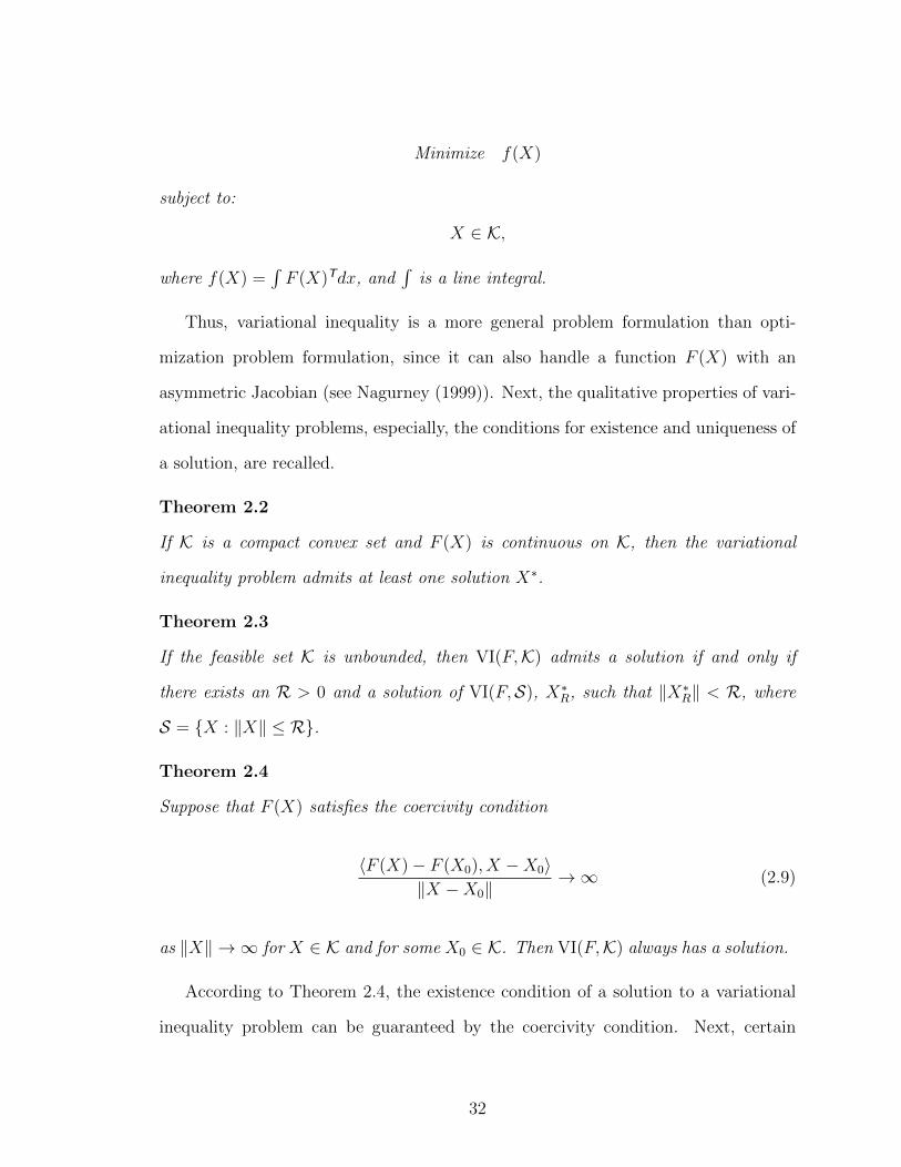
Minimize f(X)

subject to:

X ∈ K,

where f(X) =∫F (X)Tdx, and

∫is a line integral.

Thus, variational inequality is a more general problem formulation than opti-

mization problem formulation, since it can also handle a function F (X) with an

asymmetric Jacobian (see Nagurney (1999)). Next, the qualitative properties of vari-

ational inequality problems, especially, the conditions for existence and uniqueness of

a solution, are recalled.

Theorem 2.2

If K is a compact convex set and F (X) is continuous on K, then the variational

inequality problem admits at least one solution X∗.

Theorem 2.3

If the feasible set K is unbounded, then VI(F,K) admits a solution if and only if

there exists an R > 0 and a solution of VI(F,S), X∗R, such that ‖X∗R‖ < R, where

S = {X : ‖X‖ ≤ R}.

Theorem 2.4

Suppose that F (X) satisfies the coercivity condition

〈F (X)− F (X0), X −X0〉‖X −X0‖

→ ∞ (2.9)

as ‖X‖ → ∞ for X ∈ K and for some X0 ∈ K. Then VI(F,K) always has a solution.

According to Theorem 2.4, the existence condition of a solution to a variational

inequality problem can be guaranteed by the coercivity condition. Next, certain

32

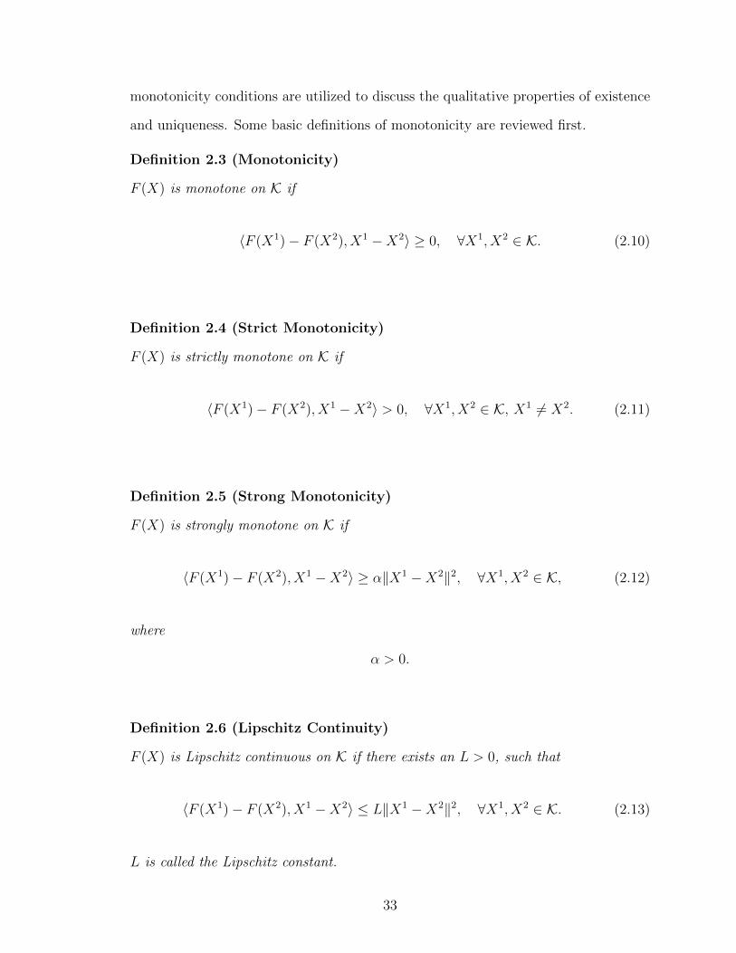
monotonicity conditions are utilized to discuss the qualitative properties of existence

and uniqueness. Some basic definitions of monotonicity are reviewed first.

Definition 2.3 (Monotonicity)

F (X) is monotone on K if

〈F (X1)− F (X2), X1 −X2〉 ≥ 0, ∀X1, X2 ∈ K. (2.10)

Definition 2.4 (Strict Monotonicity)

F (X) is strictly monotone on K if

〈F (X1)− F (X2), X1 −X2〉 > 0, ∀X1, X2 ∈ K, X1 6= X2. (2.11)

Definition 2.5 (Strong Monotonicity)

F (X) is strongly monotone on K if

〈F (X1)− F (X2), X1 −X2〉 ≥ α‖X1 −X2‖2, ∀X1, X2 ∈ K, (2.12)

where

α > 0.

Definition 2.6 (Lipschitz Continuity)

F (X) is Lipschitz continuous on K if there exists an L > 0, such that

〈F (X1)− F (X2), X1 −X2〉 ≤ L‖X1 −X2‖2, ∀X1, X2 ∈ K. (2.13)

L is called the Lipschitz constant.

33

Theorem 2.5

Suppose that F (X) is strictly monotone on K. Then the solution to the VI(F,K)

problem is unique, if one exists.

Theorem 2.6

Suppose that F (X) is strongly monotone on K. Then there exists precisely one solu-

tion X∗ to VI(F,K).

In summary of Theorems 2.2, 2.5, and 2.6, strong monotonicity of the function F

guarantees both existence and uniqueness, in the case of an unbounded feasible set

K. If the feasible set K is compact, that is, closed and bounded, the continuity of F

guarantees the existence of a solution. The strict monotonicity of F is then sufficient

to guarantee its uniqueness provided its existence.

2.2. The Relationships between Variational Inequalities and

Game Theory

In this section, some of the relationships between variational inequalities and game

theory are briefly discussed.

Nash (1950, 1951) developed noncooperative game theory, involving multiple play-

ers, each of whom acts in his/her own interest. In particular, consider a game with

m players, each player i having a strategy vector Xi = {Xi1, ..., Xin} selected from a

closed, convex set Ki ⊂ Rn. Each player i seeks to maximize his/her own utility func-

tion, Ui: K → R, where K = K1 ×K2 × . . .×Km ⊂ Rmn. The utility of player i, Ui,

depends not only on his/her own strategy vector, Xi, but also on the strategy vectors

of all the other players, (X1, . . . , Xi−1, Xi+1, . . . , Xm). An equilibrium is achieved if

no one can increase his/her utility by unilaterally altering the value of its strategy

vector. The formal definition of the Nash equilibrium is recalled as following.

34

Definition 2.7 (Nash Equilibrium)

A Nash equilibrium is a strategy vector

X∗ = (X∗1 , . . . , X∗m) ∈ K, (2.14)

such that

Ui(X∗i , X

∗i ) ≥ Ui(Xi, X

∗i ), ∀Xi ∈ Ki, ∀i, (2.15)

where X∗i = (X∗1 , . . . , X∗i−1, X

∗i+1, . . . , X

∗m).

It has been shown by Hartman and Stampacchia (1966) and Gabay and Moulin

(1980) that given continuously differentiable and concave utility functions, Ui, ∀i,

the Nash equilibrium problem can be formulated as a variational inequality problem

defined on K.

Theorem 2.7 (Variational Inequality Formulation of Nash Equilibrium)

Under the assumption that each utility function Ui is continuously differentiable and

concave, X∗ is a Nash equilibrium if and only if X∗ ∈ K is a solution of the variational

inequality

〈F (X∗), X −X∗〉 ≥ 0, X ∈ K, (2.16)

where F (X) ≡ (−∇X1U1(X), . . . ,−∇XmUm(X))T, and ∇XiUi(X) = (∂Ui(X)∂Xi1

, . . . ,

∂Ui(X)∂Xin

).

The conditions for existence and uniqueness of a Nash equilibrium are now intro-

duced. As stated in the following theorem, Rosen (1965) presented existence under

the assumptions that K is compact and each Ui is continuously differentiable.

Theorem 2.8 (Existence Under Compactness and Continuous Differentia-

bility)

Suppose that the feasible set K is compact and each Ui is continuously differentiable.

Then existence of a Nash equilibrium is guaranteed.

35

Gabay and Moulin (1980), on the other hand, relaxed the assumption of the com-

pactness of K, and proved existence of a Nash equilibrium after imposing a coercivity

condition on F (X).

Theorem 2.9 (Existence Under Coercivity)

Suppose that F (X), as given in Theorem 2.7, satisfies the coercivity condition (2.9).

Then there always exists a Nash equilibrium.

Furthermore, Karamardian (1969) demonstrated existence and uniqueness of a

Nash equilibrium under the strong monotonicity assumption.

Theorem 2.10 (Existence and Uniqueness Under Strong Monotonicity)

Assume that F (X), as given in Theorem 2.7, is strongly monotone on K. Then there

exists precisely one Nash equilibrium X∗.

Additionally, based on Theorem 2.5, uniqueness of a Nash equilibrium can be

guaranteed under the assumptions that F (X) is strictly monotone and an equilibrium

exists.

Theorem 2.11 (Uniqueness Under Strict Monotonicity)

Suppose that F (X), as given in Theorem 2.7, is strictly monotone on K. Then the

Nash equilibrium, X∗, is unique, if it exists.

2.3. Projected Dynamical Systems

In this section, the theory of projected dynamical systems (cf. Dupuis and Nagur-

ney (1993) and Nagurney and Zhang (1996)) is recalled, followed by the relationship

between projected dynamical systems and variational inequality problems. Finally,

some properties of the dynamic trajectories and the stability analysis of projected

dynamical systems are provided. All the definitions and theorems can be found in

Dupuis and Nagurney (1993) and Nagurney and Zhang (1996).

36

Definition 2.8

Given X ∈ K and v ∈ Rn, define the projection of the vector v at X (with respect to

K) by

ΠK(X, v) = limδ→0

(PK(X + δv)−X)

δ(2.17)

with PK denoting the projection map:

PK(X) = argminX′∈K‖X ′ −X‖, (2.18)

where ‖ · ‖ = 〈x, x〉.

The class of ordinary differential equations that this dissertation focuses on takes

on the following form:

X = ΠK(X,−F (X)), X(0) = X0 ∈ K, (2.19)

where X denotes the rate of change of vector X, K is closed convex set, corresponding

to the constraint set in a particular application, and F (X) is a vector field defined

on K. I refer to the ordinary differential equation in (2.19) as ODE(F,K).

The classical dynamical system, in contrast to (2.19), takes the form:

X = −F (X), X(0) = X0 ∈ K. (2.20)

Definition 2.9 (The Projected Dynamical Systems)

Define the projected dynamical system (referred to as PDS(F,K)) X0(t) : K×R 7→ K

as the family of solutions to the Initial Value Problem ( IVP) (2.19) for all X0 ∈ K.

37

Definition 2.10 (An Equilibrium Point)

The vector X∗ ∈ K is a stationary point or an equilibrium point of the projected

dynamical system PDS(F,K) if

X = 0 = ΠK(X∗,−F (X∗)). (2.21)

In other words, X∗ is a stationary point or an equilibrium point if, once the pro-

jected dynamical system is at X∗, it will remain at X∗ for all future times. Definition

2.10 demonstrates that X∗ is an equilibrium point of the projected dynamical system

PDS(F,K) if the vector field F vanishes at X∗. However, it is only true when X∗ is

an interior point of the constraint set K. When X∗ lies on the boundary of K, we

may have F (X∗) 6= 0. Note that for classical dynamical systems, the necessary and

sufficient condition for an equilibrium point is that the vector field vanish at that

point, that is, −F (X∗) = 0.

Now, I recall the equivalence between the set of equilibria of a projected dynamical

system and the set of solutions of the corresponding variational inequality problem

by presenting the following theorem (see Dupuis and Nagurney (1993)).

Theorem 2.12

Assume that K is a convex polyhedron. Then the equilibrium points of the PDS(F,K)

coincide with the solutions of VI(F,K). Hence, for X∗ ∈ K and satisfying

X = 0 = ΠK(X∗,−F (X∗)) (2.22)

also satisfies

〈F (X∗), X −X∗〉 ≥ 0, ∀X ∈ K. (2.23)

38

Before addressing the conditions for existence and uniqueness of the trajectory of

a projected dynamical system, I recall the following fundamental assumption, which

is implied by Lipschitz continuity (Definition 2.6).

Assumption 2.1

There exists a B < ∞ such that the vector field −F : Rn 7→ Rn satisfies the linear

growth condition ‖ F (X) ‖≤ B(1+ ‖ X ‖), X ∈ K, and also

〈−F (X) + F (y), X − y〉 ≤ B ‖ X − y ‖2, ∀X, y ∈ K. (2.24)

Theorem 2.13 (Existence, Uniqueness, and Continuous Dependence)

Assume the above assumption. Then

(i) For any X0 ∈ K, there exists a unique solution X0(t) to the initial value problem;

X = ΠK(X,−F (X)), X(0) = X0; (2.25)

(ii) If Xn → X0 as n→∞, then Xn(t) converges to X0(t) uniformly on every compact

set of [0,∞).

The second statement of Theorem 2.13 is sometimes called the continuous de-

pendence of the solution path to ODE(F,K) on the initial value. Therefore, the

PDS(F,K) is well-defined and inhabits K whenever Assumption 2.1 holds.

The stability of a system is defined as the ability of the system to maintain or

restore its equilibrium when acted upon by forces tending to displace it. Since the

ordinary differential equation of PDS(F,K) (2.19) has a discontinuous right-hand

side, the question of the stability of the system arises. I now recall stability concepts

for projected dynamical systems at their equilibrium points.

39

Definition 2.11 (Stability)

An equilibrium point X∗ is stable, if for any ε > 0, there exists a δ > 0, such that for

all X ∈ B(X∗, δ) and all t ≥ 0

X · t ∈ B(X∗, ε). (2.26)

The equilibrium point X∗ is unstable, if it is not stable.

B(X, r) is used to denote the open ball with radius r and center X.

Definition 2.12 (Exponential Stability)

An equilibrium point X∗ is exponentially stable, if there exists a δ > 0 and constants

B > 0 and µ > 0 such that

‖X · t−X∗‖ ≤ B‖X −X∗‖e−µt, ∀t ≥ 0, ∀X ∈ B(X∗, δ); (2.27)

X∗ is globally exponentially stable, if the above holds true for all X0 ∈ K.

Definition 2.13 (Monotone Attractor)

An equilibrium point X∗ is a monotone attractor, if there exists a δ > 0 such that for

all X ∈ B(X∗, δ),

d(X, t) =‖ X · t−X∗ ‖ (2.28)

is a nonincreasing function of t; X∗ is a global monotone attractor, if d(X, t) is

nonincreasing in t for all X ∈ K.

An equilibrium X∗ is a strictly monotone attractor, if there exists a δ > 0 such

that for all X ∈ B(X∗, δ), d(X, t) is monotonically decreasing to zero in t; X∗ is a

strictly global monotone attractor, if d(X, t) is monotonically decreasing to zero in t

for all X ∈ K.

The stability of a projected dynamical system is actually determined by the mono-

tonicity of the F (X) in the associated variational inequality problem. Next, I recall

the local and global stability directly under various monotonicity conditions.

40

Theorem 2.14 (Monotone Attractor)

Suppose that X∗ solves VI(F,K). If F (X) is locally monotone at X∗, then X∗ is

a monotone attractor for the PDS(F,K); if F (X) is monotone, then X∗ is a global

monotone attractor.

Theorem 2.15 (Strict Monotone Attractor)

Suppose that X∗ solves VI(F,K). If F (X) is locally strictly monotone at X∗, then

X∗ is a strictly monotone attractor for the PDS(F,K); if F (X) is strictly monotone

at X∗, then X∗ is a strictly global monotone attractor.

Theorem 2.16 (Exponential Stability)

Suppose that X∗ solves VI(F,K). If F (X) is locally strongly monotone at X∗, then

X∗ is exponentially stable for the PDS(F,K); if F (X) is strongly monotone at X∗,

then X∗ is a globally exponentially stable.

2.4. Multicriteria Decision-Making

The goal of multicriteria decision-making (MCDM) is to evaluate a set of alterna-

tives in terms of a number of conflicting criteria (Keeney and Raiffa (1976), Cohon

(1978), and Triantaphyllou (2000)), according to the preferences of the decision-maker

(Gal, Stewart, and Hanne (1999), and Jones, Mirrazavi, and Tamiz (2002)). In this

section, the multiobjective optimization problem and the weighted sum method are

briefly reviewed.

The multiobjective optimization problem with n decision variables can be gener-

alized as (see Marler and Arora (2004)):

Minimize G(X) = [G1(X), G2(X), . . . , Gk(X)]T (2.29)

subject to:

gj(X) ≤ 0, j = 1, 2, . . . ,m, (2.30)

41

hl(X) = 0, l = 1, 2, . . . , e, (2.31)

where k is the number of objective functions, m is the number of inequality con-

straints, e is the number of equality constraints, and X is the n-dimensional vector

of decision variables. The feasible set K1 is defined as:

K1 ≡ {X|(2.30) and (2.31) are satisfied}. (2.32)

The Pareto optimality of a solution to a multiobjective problem is defined by

Pareto (1971), as follows.

Definition 2.14 (Pareto Optimal)

A point, X∗ ∈ K1, is Pareto optimal iff there does not exist another point, X∗ ∈ K1,

such that G(X) ≤ G(X∗), and Gi(X) < Gi(X∗) for at least one function.

The weighted sum method, which is the most common approach to multiobjective

optimization problems (see Marler and Arora (2004)), is as following. Associated with

a vector of weights, denoted by w, representing the decision-maker’s preferences, the

multiobjective objective function (2.29) can be expressed as:

Γ =k∑i=1

wiGi(X). (2.33)

As noted by Zadeh (1963), the optimal solution to (2.33) is Pareto optimal if all of

the weights are positive.

2.5. Algorithms

In this section, I review the algorithms. The Euler method, which is based on the

general iterative scheme of Dupuis and Nagurney (1993), and the modified projection

method of Korpelevich (1977) are presented.

42

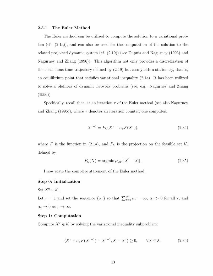
2.5.1 The Euler Method

The Euler method can be utilized to compute the solution to a variational prob-

lem (cf. (2.1a)), and can also be used for the computation of the solution to the

related projected dynamic system (cf. (2.19)) (see Dupuis and Nagurney (1993) and

Nagurney and Zhang (1996)). This algorithm not only provides a discretization of

the continuous time trajectory defined by (2.19) but also yields a stationary, that is,

an equilibrium point that satisfies variational inequality (2.1a). It has been utilized

to solve a plethora of dynamic network problems (see, e.g., Nagurney and Zhang

(1996)).

Specifically, recall that, at an iteration τ of the Euler method (see also Nagurney

and Zhang (1996)), where τ denotes an iteration counter, one computes:

Xτ+1 = PK(Xτ − ατF (Xτ )), (2.34)

where F is the function in (2.1a), and PK is the projection on the feasible set K,

defined by

PK(X) = argminX′∈K‖X′ −X‖. (2.35)

I now state the complete statement of the Euler method.

Step 0: Initialization

Set X0 ∈ K.

Let τ = 1 and set the sequence {ατ} so that∑∞

τ=1 ατ = ∞, ατ > 0 for all τ , and

ατ → 0 as τ →∞.

Step 1: Computation

Compute Xτ ∈ K by solving the variational inequality subproblem:

〈Xτ + ατF (Xτ−1)−Xτ−1, X −Xτ 〉 ≥ 0, ∀X ∈ K. (2.36)

43

Step 2: Convergence Verification

If max |Xτl − Xτ−1

l | ≤ ε, for all l, with ε > 0, a pre-specified tolerance, then stop;

otherwise, set τ := τ + 1, and go to Step 1.

The VI subproblem (2.36) is actually a quadratic programming problem. It can

be solved by the exact equilibration algorithm of Dafermos and Sparrow (1969) when

it has a special network structure. In this dissertation, where appropriate, I also

explore the network structure. This algorithm has been applied to many different

applications of networks with special structure (cf. Nagurney and Zhang (1996) and

Nagurney (1999)). See also Nagurney and Zhang (1997) for an application to fixed-

demand traffic network equilibrium problems. The exact equilibration algorithm is

used in Chapters 5 and 6 to solve some subproblems induced in the Euler method for

fixed-demand supply chain network problems with outsourcing.

An assumption is recalled, followed by the convergence conditions of the Euler

method in Theorem 2.17 and Corollary 2.1.

Assumption 2.2

Suppose we fix an initial condition X0 ∈ K and define the sequence {Xτ , τ ∈ N} by

(2.34). We assume the following conditions:

1.∑∞

i=0 ai =∞, ai > 0, ai → 0 as i→∞.

2. d(Fτ (x), F (x))→ 0 uniformly on compact subsets of K as τ →∞.

3. Define φy to be the unique solution to X = ΠK(X,−F (X)) that satisfies φy(0) =

y ∈ K. The ω-limit set of K

ω(K) = ∪y∈K ∩t≥0 ∪s≥t{φy(s)}

is contained in the set of stationary points of X = ΠK(X,−F (X)).

4. The sequence {Xτ , τ ∈ N} is bounded.

44

5. The solution to X = ΠK(X,−F (X)) are stable in the sense that given any

compact set K1 there exists a compact set K2 such that ∪y∈K∩K1 ∪t≥0 {φy(t)} ⊂ K2.

Theorem 2.17

Let S denote the set of stationary point of the projected dynamical system (2.19),

equivalently, the set of solutions to the variational inequality problem (2.1a). Assume

Assuption 2.1 and Assumption 2.2. Suppose {Xτ , τ ∈ N} is the scheme generated by

(2.34). Then d(Xτ , S)→ 0 as τ →∞, where d(Xτ , S)→ 0 = infX∈S‖Xτ −X‖.

Corollary 2.1

Assume the conditions of Theorem 2.17, and also that S consists of a finite set of

points. Then limτ→∞Xτ exists and equals to a solution to the variational inequality.

Theorem 2.17 indicates that Assumption 2.2 is the elementary condition under

which the Euler method (2.34) converges. Proposition 2.3 and Proposition 2.4 below

suggest some alternative conditions that are better known in variational inequality

theory as sufficient conditions for Part 3 and Part 5 of Assumption 2.2.

Proposition 2.3

If the vector field F (X) is strictly monotone at some solution X∗ to the variational

inequality problem (2.1a), then Part 3 of Assumption 2.2 holds true.

Proposition 2.4

If the vector field F (X) is monotone at some solution X∗ to the variational inequality

problem (2.1a), then Part 5 of Assumption 2.2 holds true.

In the subsequent chapters, as appropriate, I adapt the convergence proofs to

specific supply chain network applications.

2.5.2 The Modified Projection Method

The modified projection method of Korpelevich (1977) can be utilized to solve a

variational inequality problem in standard form (cf. (2.1a)). This method is guaran-

teed to converge if the monotonicity (cf. (2.10)) and Lipschitz continuity (cf. (2.13))

45

of the function F that enters the variational inequality (cf. (2.1a)) can be satisfied,

and a solution to the variational inequality exists.

I now recall the modified projection method, and let τ denote an iteration counter.

Step 0: Initialization

Set X0 ∈ K. Let τ = 1 and let α be a scalar such that 0 < α ≤ 1L

, where L is the

Lipschitz continuity constant (cf. (2.13)).

Step 1: Computation

Compute Xτ by solving the variational inequality subproblem:

〈Xτ + αF (Xτ−1)−Xτ−1, X − Xτ 〉 ≥ 0, ∀X ∈ K. (2.37)

Step 2: Adaptation

Compute Xτ by solving the variational inequality subproblem:

〈Xτ + αF (Xτ )−Xτ−1, X −Xτ 〉 ≥ 0, ∀X ∈ K. (2.38)

Step 3: Convergence Verification

If max |Xτl −Xτ−1

l | ≤ ε, for all l, with ε > 0, a prespecified tolerance, then stop; else,

set τ := τ + 1, and go to Step 1.

Theorem 2.18 (Convergence of the Modified Projection Method)

If F (X) is monotone and Lipschitz continuous (and a solution exists), the modified

projection algorithm converges to a solution of variational inequality (2.1a).

In the following chapters, I derive the variational inequality formulations and

the projected dynamical systems of the supply chain network models with quality

competition with application to information asymmetry, production differentiation,

outsourcing, and supplier selection. The computational algorithms introduced in this

46

chapter, which are the Euler method and the modified projection method, are also

adapted accordingly.

47

CHAPTER 3

A SUPPLY CHAIN NETWORK MODEL WITHINFORMATION ASYMMETRY IN QUALITY, MINIMUM

QUALITY STANDARDS, AND QUALITYCOMPETITION

In this chapter, I construct a supply chain network model with information asym-

metry between firms and consumers in product quality. The competing, profit-

maximizing firms with, possibly, multiple manufacturing plants which may be located

on-shore or off-shore, are aware of their quality levels but do not have differentiated

brands or labels to distinguish their products from their competitors’. Therefore,

consumers at the demand markets view the products as well as their quality levels as

homogeneous. Such a framework is relevant to products ranging from certain foods

to pharmaceuticals.

In this model, firms compete with one another in both the shipment amounts pro-

duced as well as the quality levels at their manufacturing plants with the objective

of profit maximization. Quality is associated not only with the manufacturing plants

but also tracked through the transportation process, which is assumed to preserve the

product quality. I propose both the equilibrium model, with the equivalent variational

inequality formulation, and its dynamic counterpart, using projected dynamical sys-

tems theory, and demonstrate how minimum quality standards can be incorporated

into the framework. Both theoretical results, in the form of existence and uniqueness

results as well as stability analysis, are presented. The Euler method (cf. Section

2.5.1) is used to solve the model, and the convergence results are also given. The

numerical examples, accompanied by sensitivity analysis, reveal interesting results

48

and insights for firms, consumers, as well as policy-makers, who impose the minimum

quality standards.

This chapter is based on Nagurney and Li (2014a), and is organized as follows.

In Section 3.1, I present both the static models (without and with minimum qual-

ity standards), along with their variational inequality formulations, as well as the

dynamic version using projected dynamical systems theory. In Section 3.2, I then

provide qualitative properties of the equilibrium solutions and establish that the set

of stationary points of the projected dynamical systems formulation coincides with

the set of solutions to the corresponding variational inequality problem. In Section

3.3, I describe the closed form expressions for the Euler method applied in computing

the equilibrium product shipments and quality levels, and establish convergence. In

Section 3.4, I provide numerical examples and conduct sensitivity analyses, which

yield valuable insights for firms, consumers, and policy-makers. In Section 3.5, I

summarize the results and present the conclusions.

3.1. The Supply Chain Network Model with Information

Asymmetry in Quality and Quality Competition

In this section, I construct the supply chain network equilibrium model in which

the firms compete in product quantities and quality levels and there is information

asymmetry in quality. I first consider the case without minimum quality standards

and them demonstrate how standards can be incorporated. Next, the dynamic coun-

terpart of the latter is developed, which contains the former as a special case. The

static equilibrium model(s) are given in Section 3.2.1 and the dynamic version in

Section 3.2.2.

49

3.1.1 The Equilibrium Model Without and With Minimum Quality Stan-

dards

I first present the model without minimum quality standards and then show how

it can be extended to include minimum quality standards, which are useful policy

instruments in practice.

I consider I firms, with a typical firm denoted by i, which compete with one

another in a noncooperative Cournot-Nash manner in the production and distribution

of the product. Each firm i has, at its disposal, ni manufacturing plants. The firms

determine the quantities to produce at each of their manufacturing plants and the

quantities to ship to the nR demand markets. They also control the quality level of

the product at each of their manufacturing plants. Information asymmetry occurs in

that the firms are aware of the quality levels of the product produced at each of their

manufacturing plants but the consumers are only aware of the average quality levels

of the product at the demand markets.

I consider the supply chain network topology depicted in Figure 3.1. The top

nodes correspond to the firms, the middle nodes to the manufacturing plants, and

the bottom nodes to the common demand markets. I assume that the demand at

each demand market is positive; otherwise, the demand market (node) will be removed

from the supply chain network.

In Figure 3.1, the first set of links connecting the top two tiers of nodes corresponds

to the process of manufacturing at each of the manufacturing plants of firm i; i =

1, . . . , I. Such plants are denoted by M1i , . . . ,M

nii , respectively, for firm i, with a

typical one denoted by M ji ; j = 1, . . . , ni. The manufacturing plants may be located

not only in different regions of a country but also in different countries. The next

set of links connecting the two bottom tiers of the supply chain network corresponds

to transportation links joining the manufacturing plants with the demand markets,

with a typical demand market denoted by Rk; k = 1, . . . , nR.

50

� ��R1 · · · RnR� ��

M11� ��· · · � ��Mn1

1 · · · M1I� ��· · · � ��MnI

I

��

@@@@R

��

@@@@R

� ��1 � ��I· · ·Firm 1 Firm I

\\\\\\\\\

HHHHHHHHHHHHHHHHH

llllllllll

· · ·

��

,,,,,,,,,,

�� ??� RjR

Figure 3.1. The Supply Chain Network Topology with Multiple ManufacturingPlants

The nonnegative product amount produced at firm i’s manufacturing plant M ji

and shipped to demand market Rk is denoted by Qijk; i = 1, . . . , I; j = 1, . . . , ni;

k = 1 . . . , nR. For each firm i, I group its Qijks into the vector Qi ∈ RninR+ , and then

group all such vectors for all firms into the vector Q ∈ R∑Ii=1 ninR

+ .

The nonnegative production output of firm i’s manufacturing plant M ji is denoted

by sij, the demand for the product at demand market Rk is denoted by dk; k =

1, . . . , nR, and the quality level or, simply, quality, of the product produced by firm

i’s manufacturing plant M ji is denoted by qij. Note that different manufacturing

plants owned by a firm may have different quality levels. This is highly reasonable

since, for example, different plants may have different resources available in terms of

skilled labor and facilities as well as labor expertise and even infrastructure.

The output at firm i’s manufacturing plant M ji and the demand for the product at

each demand market Rk must satisfy, respectively, the conservation of flow equations

(3.1) and (3.2):

sij =

nR∑k=1

Qijk, i = 1, . . . , I; j = 1, . . . , ni, (3.1)

51

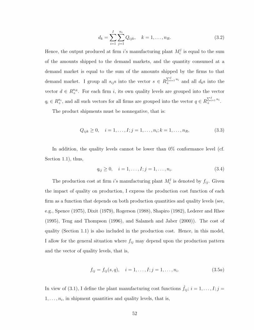
dk =I∑i=1

ni∑j=1

Qijk, k = 1, . . . , nR. (3.2)

Hence, the output produced at firm i’s manufacturing plant M ji is equal to the sum

of the amounts shipped to the demand markets, and the quantity consumed at a

demand market is equal to the sum of the amounts shipped by the firms to that

demand market. I group all sijs into the vector s ∈ R∑Ii=1 ni

+ and all dks into the

vector d ∈ RnR+ . For each firm i, its own quality levels are grouped into the vector

qi ∈ Rni+ , and all such vectors for all firms are grouped into the vector q ∈ R

∑Ii=1 ni

+ .

The product shipments must be nonnegative, that is:

Qijk ≥ 0, i = 1, . . . , I; j = 1, . . . , ni; k = 1, . . . , nR, (3.3)

In addition, the quality levels cannot be lower than 0% conformance level (cf.

Section 1.1), thus,

qij ≥ 0, i = 1, . . . , I; j = 1, . . . , ni. (3.4)

The production cost at firm i’s manufacturing plant M ji is denoted by fij. Given

the impact of quality on production, I express the production cost function of each

firm as a function that depends on both production quantities and quality levels (see,

e.g., Spence (1975), Dixit (1979), Rogerson (1988), Shapiro (1982), Lederer and Rhee

(1995), Teng and Thompson (1996), and Salameh and Jaber (2000)). The cost of

quality (Section 1.1) is also included in the production cost. Hence, in this model,

I allow for the general situation where fij may depend upon the production pattern

and the vector of quality levels, that is,

fij = fij(s, q), i = 1, . . . , I; j = 1, . . . , ni. (3.5a)

In view of (3.1), I define the plant manufacturing cost functions fij; i = 1, . . . , I; j =

1, . . . , ni, in shipment quantities and quality levels, that is,

52

fij = fij(Q, q) ≡ fij(s, q). (3.5b)

Moreover, given the impact of quality on transportation (cf. Floden, Barthel,

and Sorkina (2010) and Saxin, Lammgard, and Floden (2005) and the references

therein), I also associate quality with respect to the distribution/transport activities

of the products to the demand markets. I accomplish this by having the transporta-

tion/distribution functions depend explicitly on both flows and quality levels, with

the assumption of quality preservation, that is, the product will be delivered at the

same quality level that it was produced at. Let cijk denote the total transportation

cost associated with shipping the product produced at firm i’s manufacturing plant

M ji to demand market Rk, that is,

cijk = cijk(Q, q), i = 1, . . . , I; j = 1, . . . , ni; k = 1, . . . , nR. (3.6)

Note that, according to (3.6), the transportation cost is such that the quality of the

product is not degraded as it undergoes the shipment process. Transportation cost

functions in both quantities and quality levels were utilized by Nagurney and Wolf

(2014), Saberi, Nagurney, and Wolf (2014), and Nagurney et al. (2014) but in the

context of Internet applications and not supply chains.

Since the products of the I firms are, in effect, homogeneous, common resources

and technologies may be utilized in the processes of manufacturing and transporta-

tion. In this model, in order to capture the competition for resources and technologies

on the supply side, I allow for general production cost functions, which may depend

on the entire production pattern s and the entire vector of quality levels q (cf. (3.5a)),

and general transportation cost functions, which may depend on the vectors Q and

q (cf. (3.6)). These cost functions measure not only the monetary costs in the cor-

responding processes, but also other important factors, such as the time spent in

conforming the processes. Such general production and transportation cost functions

53

in both quantities and quality levels are utilized, for the first time, in a supply chain

context. The production cost functions (3.5a) and the transportation functions (3.6)

are assumed to be convex and twice continuously differentiable.

Since firms do not differentiate the products as well as their quality levels, con-

sumers’ perception of the quality of all such products, which may come from different

firms, is the average quality level of all products, qk; k = 1, . . . , nR, where

qk =

∑Ii=1

∑nij=1Qijkqij

dk, k = 1, . . . , nR (3.7)

with the average (perceived) quality levels grouped into the vector q ∈ RnR+ . Here,

I utilize the average quality as proposed by the Nobel laureate George Akerlof (see

Akerlof (1970)) and further developed by the Nobel laureates Stiglitz (1987) and

Spence (1975). In this model, the quality of a product is not directly observable by

consumers, but it can be estimated by the average quality of all such products in the

same demand market (cf. Nagurney, Li, and Nagurney (2014)). This average quality

can be conveyed among consumers through word of mouth, their own consumption

experiences, advertising, etc.

The demand price at demand market Rk is denoted by ρk. Consumers located at

the demand markets, which are spatially separated, respond not only to the quantities

available of the products but also to their quality levels. Recall that Kaya and Ozer

(2009) and Kaya (2011) considered demand functions in price and quality, which are

of the following form: q = a − bp + e + ε, where e is the quality effort. Xie et al.

(2011) utilized a demand function in the investigation of quality investment, of the

form D = a+αx−βp, where x is quality. Anderson and de Palma (2001) captured the

utility u of each consumer as u = q−p+ε in their research on asymmetric oligopolies,

with q being quality. In addition, Banker, Khosla, and Sinha (1998) considered a

duopoly case and utilized a demand function given by qi = kiα−βpi+γpj+λxi−µxj,

where x denotes quality. In the model in this chapter, because the products are

54

homogeneous, the demand price function of all such products at a demand market

depends, in general, upon the entire demand pattern, as well as on the average quality

levels at all the demand markets, that is,

ρk = ρk(d, q), k = 1, . . . , nR. (3.8a)

The generality of this expression enables modeling and application flexibility. Each

demand price function is, typically, assumed to be monotonically decreasing in prod-

uct quantity but increasing in terms of the average product quality. Demand functions

that are functions of the prices and the average quality levels were also used by Ak-

erlof (1970). Therein the producers, in the form of a supply market, are aware of

their product quality levels (cf. (3.5a)), while consumers at the demand markets are

aware only of the average quality levels. However, multiple manufacturing plants,

transportation, and multiple demand markets are not considered in Akerlof (1970),

and, the profit-maximizing behavior of individual, competing firms, as in this chapter,

is not modeled.

In light of (3.2) and (3.7), one can define the demand price function ρk; k =

1, . . . , nR, in quantities and quality levels of the firms, so that

ρk = ρk(Q, q) ≡ ρk(d, q), k = 1, . . . , nR. (3.8b)

Functions (3.8a and b) are not limited to linear demand price functions, and they are

assumed to be continuous and twice continuously differentiable.

The strategic variables of firm i are its product shipments {Qi} and its quality

levels qi. The profit/utility Ui of firm i; i = 1, . . . , I, is given by:

Ui =

nR∑k=1

ρk(d, q)

ni∑j=1

Qijk −ni∑j=1

fij(s, q)−nR∑k=1

ni∑j=1

cijk(Q, q), (3.9a)

55

which is the difference between its total revenue and its total costs (production and

transportation). By making use of (3.5b) and (3.8b), (3.9a) is equivalent to

Ui =

nR∑k=1

ρk(Q, q)

ni∑j=1

Qijk −ni∑j=1

fij(Q, q)−nR∑k=1

ni∑j=1

cijk(Q, q). (3.9b)

In view of (3.1) - (3.9b), one may write the profit as a function solely of the

product shipment pattern and quality levels, that is,

U = U(Q, q), (3.10)

where U is the I-dimensional vector with components: {U1, . . . , UI}.

Let Ki denote the feasible set corresponding to firm i, where Ki ≡ {(Qi, qi)|Qi ≥

0, and qi ≥ 0} and define K ≡∏I

i=1Ki.

I consider Cournot-Nash competition, in which the I firms produce and deliver

their product in a noncooperative fashion, each one trying to maximize its own profit.

They seek to determine a nonnegative product shipment and quality level pattern

(Q∗, q∗) ∈ K for which the I firms will be in a state of equilibrium as defined below

(cf. Definition 2.7).

Definition 3.1: A Supply Chain Network Cournot-Nash Equilibrium with

Information Asymmetry in Quality

A product shipment and quality level pattern (Q∗, q∗) ∈ K is said to constitute a supply

chain network Cournot-Nash equilibrium with information asymmetry in quality if for

each firm i; i = 1, . . . , I,

Ui(Q∗i , q∗i , Q

∗i , q∗i ) ≥ Ui(Qi, qi, Q

∗i , q∗i ), ∀(Qi, qi) ∈ Ki, (3.11)

where Q∗i ≡ (Q∗1, . . . , Q∗i−1, Q

∗i+1, . . . , Q

∗I) and q∗i ≡ (q∗1, . . . , q

∗i−1, q

∗i+1, . . . , q

∗I ).

56

According to (3.11), an equilibrium is established if no firm can unilaterally im-

prove upon its profits by selecting an alternative vector of product shipments and

quality level of its product.

I now present alternative variational inequality formulations of the above supply

chain network Cournot-Nash equilibrium in the following theorem.

Theorem 3.1: Variational Inequality Formulations

Assume that for each firm i the profit function Ui(Q, q) is concave with respect to the

variables in Qi and qi, and is continuous and continuously differentiable. Then the

product shipment and quality pattern (Q∗, q∗) ∈ K is a supply chain network Cournot-

Nash equilibrium with quality information asymmetry according to Definition 3.1 if

and only if it satisfies the variational inequality

−I∑i=1

ni∑j=1

nR∑k=1

∂Ui(Q∗, q∗)

∂Qijk

× (Qijk −Q∗ijk)−I∑i=1

ni∑j=1

∂Ui(Q∗, q∗)

∂qij× (qij − q∗ij) ≥ 0,

∀(Q, q) ∈ K, (3.12)

that is,

I∑i=1

ni∑j=1

nR∑k=1

[−ρk(Q∗, q∗)−

nR∑l=1

∂ρl(Q∗, q∗)

∂Qijk

ni∑h=1

Q∗ihl +

ni∑h=1

∂fih(Q∗, q∗)

∂Qijk

+

ni∑h=1

nR∑l=1

∂cihl(Q∗, q∗)

∂Qijk

]× (Qijk −Q∗ijk)

+I∑i=1

ni∑j=1

[−

nR∑k=1

∂ρk(Q∗, q∗)

∂qij

ni∑h=1

Q∗ihk +

ni∑h=1

∂fih(Q∗, q∗)

∂qij+

ni∑h=1

nR∑k=1

∂cihk(Q∗, q∗)

∂qij

]×(qij − q∗ij) ≥ 0, ∀(Q, q) ∈ K; (3.13)

equivalently, (d∗, s∗, Q∗, q∗) ∈ K1 is an equilibrium production, shipment, and quality

level pattern if and only if it satisfies the variational inequality

nR∑k=1

[−ρk(d∗, q∗)]× (dk − d∗k) +I∑i=1

ni∑j=1

[ni∑h=1

∂fih(s∗, q∗)

∂sij

]× (sij − s∗ij)

57

+I∑i=1

ni∑j=1

nR∑k=1

[−

nR∑l=1

∂ρl(d∗, q∗)

∂Qijk

ni∑h=1

Q∗ihl +

ni∑h=1

nR∑l=1

∂cihl(Q∗, q∗)

∂Qijk


+I∑i=1

ni∑j=1

[−

nR∑k=1

∂ρk(Q∗, q∗)

∂qij

ni∑h=1

Q∗ihk +

ni∑h=1

∂fih(s∗, q∗)

∂qij+

ni∑h=1

nR∑k=1

∂cihk(Q∗, q∗)

∂qij

]×(qij − q∗ij) ≥ 0, ∀(d, s,Q, q) ∈ K1, (3.14)

where K1 ≡ {(d, s,Q, q)|Q ≥ 0, q ≥ 0, and (3.1), (3.2), and (3.7) hold}.

Proof: (3.12) follows directly from Gabay and Moulin (1980) and Dafermos and

Nagurney (1987), as given in Theorem 2.7. For firm i’s manufacturing plant M ji ;

i = 1, . . . , I; j = 1, . . . , ni and demand market Rk; k = 1, . . . , nR:

−∂Ui(Q, q)∂Qijk

= −∂[∑nR

l=1 ρl(Q, q)∑ni

h=1Qihl −∑ni

h=1 fih(Q, q)−∑ni

h=1

∑nRl=1 cihl(Q, q)]

∂Qijk

= −nR∑l=1

∂[ρl(Q, q)∑ni

h=1 Qihl]

∂Qijk

+

ni∑h=1

∂fih(Q, q)

∂Qijk

+

ni∑h=1

nR∑l=1

∂cihl(Q, q)

∂Qijk

= −ρk(Q, q)−nR∑l=1

∂ρl(Q, q)

∂Qijk

ni∑h=1

Qihl +

ni∑h=1

∂fih(Q, q)

∂Qijk

+

ni∑h=1

nR∑l=1

∂cihl(Q, q)

∂Qijk

. (3.15)

Also, for firm i’s manufacturing plant M ji ; i = 1, . . . , I; j = 1, . . . , ni:

−∂Ui(Q, q)∂qij

= −∂[∑nR

k=1 ρk(Q, q)∑ni

h=1Qihk −∑ni

h=1 fih(Q, q)−∑ni

h=1

∑nRk=1 cihk(Q, q)]

∂qij

= −nR∑k=1

∂ρk(Q, q)

∂qij

ni∑h=1

Qihk +

ni∑h=1

∂fih(Q, q)

∂qij+

ni∑h=1

nR∑k=1

∂cihk(Q, q)

∂qij. (3.16)

Thus, variational inequality (3.13) is immediate. In addition, by re-expressing the

production cost functions and the demand price functions in (3.15) and (3.16) as in

(3.5b) and (3.8b) and using the conservation of flow equations (3.1) and (3.2) and

∂fih(s,q)∂Qijk

= ∂fih(s,q)∂sij

∂sij∂Qijk

, the equivalence of variational inequalities (3.13) and (3.14)

holds true.2

58

I now describe an extension of the above framework that incorporates minimum

quality standards. I integrate the framework with minimum quality standards and

the framework without, and present the equilibrium conditions of both through a

unified variational inequality formulation.

I retain the above notation, firm behavior, and constraints, but now nonnegative

lower bounds on the quality levels at the manufacturing plants are imposed, denoted

by qij

; i = 1, . . . , I; j = 1, . . . , ni so that (3.4) is replaced by:

qij ≥ qij

i = 1, . . . , I; j = 1, . . . , ni (3.17)

with the understanding that, if the lower bounds are all identically equal to zero, then

(3.17) collapses to (3.4) and, if the lower bounds are positive, then they represent

minimum quality standards.

I define a new feasible set K2 ≡ {(Q, q)|Q ≥ 0 and (3.17) holds}. Then the follow-

ing Corollary is immediate.

Corollary 3.1: Variational Inequality Formulations with Minimum Quality

Standards

Assume that for each firm i the profit function Ui(Q, q) is concave with respect to

the variables in Qi and qi, and is continuous and continuously differentiable. Then

the product shipment and quality pattern (Q∗, q∗) ∈ K2 is a supply chain network

Cournot-Nash equilibrium with quality information asymmetry in the presence of min-

imum quality standards if and only if it satisfies the variational inequality

−I∑i=1

ni∑j=1

nR∑k=1

∂Ui(Q∗, q∗)

∂Qijk

× (Qijk −Q∗ijk)−I∑i=1

ni∑j=1

∂Ui(Q∗, q∗)

∂qij× (qij − q∗ij) ≥ 0,

∀(Q, q) ∈ K2, (3.18)

59

that is,

I∑i=1

ni∑j=1

nR∑k=1

[−ρk(Q∗, q∗)−

nR∑l=1

∂ρl(Q∗, q∗)

∂Qijk

ni∑h=1

Q∗ihl +

ni∑h=1

∂fih(Q∗, q∗)

∂Qijk

+

ni∑h=1

nR∑l=1

∂cihl(Q∗, q∗)

∂Qijk


+I∑i=1

ni∑j=1

[−

nR∑k=1

∂ρk(Q∗, q∗)

∂qij

ni∑h=1

Q∗ihk +

ni∑h=1

∂fih(Q∗, q∗)

∂qij+

ni∑h=1

nR∑k=1

∂cihk(Q∗, q∗)

∂qij

]×(qij − q∗ij) ≥ 0, ∀(Q, q) ∈ K2. (3.19)

Variational inequality (3.19) contains variational inequality (3.13) as a special case

when the minimum quality standards are all zero, and it will play a crucial role in

the next section when the underlying dynamics associated with the firms’ adjustment

processes in product shipments and quality levels is described.

I now put variational inequality (3.19) into standard form (cf. (2.1a)): determine

X∗ ∈ K where X is a vector in RN , F (X) is a continuous function such that F (X) :

X 7→ K ⊂ RN , and

〈F (X∗), X −X∗〉 ≥ 0, ∀X ∈ K, (3.20)

where 〈·, ·〉 is the inner product in the N -dimensional Euclidean space, and K is closed

and convex. I define the vector X ≡ (Q, q) and the vector F (X) ≡ (F 1(X), F 2(X)).

Also, here N =∑I

i=1 ninR+∑I

i=1 ni. F1(X) consists of components F 1

ijk = −∂Ui(Q,q)∂Qijk

;

i = 1, . . . , I; j = 1, . . . , ni; k = 1, . . . , nR, and F 2(X) consist of components F 2ij =

−∂Ui(Q,q)∂qij

; i = 1, . . . , I; j = 1, . . . , ni. In addition, I define the feasible set K ≡ K2.

Hence, (3.19) can be put into standard form (2.1a).

60

3.1.2 The Dynamic Model

I now describe the underlying dynamics for the evolution of product shipments and

quality levels under information asymmetry in quality until the equilibrium satisfying

variational inequality (3.19) is achieved.

Observe that, for a current vector of product shipments and quality levels at time

t, X(t) = (Q(t), q(t)), −F 1ijk(X(t)) = ∂Ui(Q(t),q(t))

∂Qijkis the marginal utility (profit) of firm

i with respect to the volume produced at its manufacturing plant j and distributed to

demand market Rk. −F 2ij(X(t)) = ∂Ui(Q(t),q(t))

∂qijis firm i’s marginal utility with respect

to the quality level of its manufacturing plant j. In this framework, the rate of change

of the product shipment between firm i’s manufacturing plant j and demand market

Rk is in proportion to −F 1ij(X), as long as the product shipment Qijk is positive.

Namely, when Qijk > 0,

Qijk =∂Ui(Q, q)

∂Qijk

, (3.21)

where Qijk denotes the rate of change of Qijk. However, when Qijk = 0, the non-

negativity condition (3.3) forces the product shipment Qijk to remain zero when

∂Ui(Q,q)∂Qijk

≤ 0. Hence, one is only guaranteed of having possible increases of the ship-

ment, that is, when Qijk = 0,

Qijk = max{0, ∂Ui(Q, q)∂Qijk

}. (3.22)

One may write (3.21) and (3.22) concisely as:

Qijk =

∂Ui(Q,q)∂Qijk

, if Qijk > 0

max{0, ∂Ui(Q,q)∂Qijk

}, if Qijk = 0.(3.23)

As for the quality levels, when qij > qij

, then

qij =∂Ui(Q, q)

∂qij, (3.24)

61

where qij denotes the rate of change of qij; when qij = qij

,

qij = max{qij,∂Ui(Q, q)

∂qij}, (3.25)

since qi cannot be lower than qij

according to the feasible set K = K2.

Combining (3.24) and (3.25), one may write:

qij =

∂Ui(Q,q)∂qij

, if qij > qij

max{qij, ∂Ui(Q,q)

∂qij}, if qij = q

ij.

(3.26)

Applying (3.23) to all firm and manufacturing plant pairs (i, j); i = 1, . . . , I; j =

1, . . . , ni and all demand markets Rk; k = 1, . . . , nR, and then applying (3.26) to all

firm and manufacturing plant pairs (i, j); i = 1, . . . , I; j = 1, . . . , ni, and combining

the resultants, yields the following pertinent ordinary differential equation (ODE) (cf.

(2.19)) for the adjustment processes of the product shipments and quality levels, in

vector form:

X = ΠK(X,−F (X)), (3.27)

where −F (X) = ∇U(Q, q), and ∇U(Q, q) is the vector of marginal utilities as de-

scribed above.

I now further interpret ODE (3.27) in the context of the supply chain network

competition model with information asymmetry in quality. First, observe that ODE

(3.27) guarantees that the product shipments are always nonnegative and the quality

levels never go below the minimum quality standards. In addition, ODE (3.27) states

that the rate of change of the product shipments and the quality levels is greatest

when the firm’s marginal utilities are greatest. If the marginal utility of a firm with

respect to its quality level is positive, then the firm will increase its quality level; if

it is negative, then it will decrease the quality level, and the quality levels will also

never be outside their lower bounds. A similar adjustment behavior holds for the

62

firms in terms of their product shipments. This type of behavior is rational from an

economic standpoint. Therefore, ODE (3.27) corresponds to reasonable continuous

adjustment processes for the supply chain network competition model with informa-

tion asymmetry in quality.

3.2. Qualitative Properties

Since ODE (3.27) is nonstandard due to its discontinuous right-hand side, I further

discuss the existence and uniqueness of (3.27). The fundamental theory with regards

to existence and uniqueness of projected dynamical systems is provided in Theorem

2.13.

As given in Theorem 2.12, the necessary and sufficient condition for a product

shipment and quality level pattern X∗ = (Q∗, q∗) to be a supply chain network equi-

librium with information asymmetry in quality, according to Definition 3.1, is that

X∗ = (Q∗, q∗) is a stationary point of the adjustment processes defined by ODE

(3.27), that is, X∗ is the point at which X = 0.

I now investigate whether, and, under what conditions, the dynamic adjustment

processes defined by (3.27) approach a Cournot-Nash equilibrium. Recall that Lip-

schitz continuity of F (X) (cf. Definition 2.6) guarantees the existence of a unique

solution to (2.19) (cf. Theorem 2.13), where X0(t) satisfies ODE (2.19) with initial

shipment and quality level pattern (Q0, q0).

In addition, if the utility functions are twice differentiable and the Jacobian matrix

of F (X), denoted by ∇F (X), is positive-definite, then the corresponding F (X) is

strictly monotone, and the solution to variational inequality (3.20) is unique, if it

exists, according to Theorem 2.5.

Assumption 3.1

Suppose that in the supply chain network model with information asymmetry in quality

there exists a sufficiently large M , such that for any (i, j, k),

63

∂Ui(Q, q)

∂Qijk

< 0, (3.28)

for all shipment patterns Q with Qijk ≥ M and that there exists a sufficiently large

M , such that for any (i, j),

∂Ui(Q, q)

∂qij< 0, (3.29)

for all quality level patterns q with qij ≥ M ≥ qij

.

I now give an existence result.

Proposition 3.1

Any supply chain network problem with information asymmetry in quality that sat-

isfies Assumption 3.1 possesses at least one equilibrium shipment and quality level

pattern satisfying variational inequality (3.19) (or (3.20)).

Proof: The proof follows from Theorem 2.3 and Proposition 1 in Zhang and Nagurney

(1995). 2

For completeness, a uniqueness result is now presented, see also Theorem 2.5.

Proposition 3.2

Suppose that F is strictly monotone at any equilibrium point of the variational in-

equality problem defined in (3.20). Then it has at most one equilibrium point.

In addition, an existence and uniqueness result is recalled (cf. Theorem 2.6).

Theorem 3.2

Suppose that F is strongly monotone. Then there exists a unique solution to varia-

tional inequality (3.20); equivalently, to variational inequality (3.19).

Moreover, the stability properties of the utility gradient processes are summarized

(cf. Theorems 2.14, 2.15, and 2.16), under various monotonicity conditions on the

marginal utilities (cf. Definitions 2.3, 2.4, and 2.5).

64

Theorem 3.3

(i). If F (X) is monotone, then every supply chain network equilibrium with infor-

mation asymmetry, X∗, provided its existence, is a global monotone attractor for the

projected dynamical system. If F (X) is locally monotone at X∗, then it is a monotone

attractor for the projected dynamical system.

(ii). If F (X) is strictly monotone, then there exists at most one supply chain net-

work equilibrium with information asymmetry in quality, X∗. Furthermore, given

existence, the unique equilibrium is a strictly global monotone attractor for the pro-

jected dynamical system. If F (X) is locally strictly monotone at X∗, then it is a

strictly monotone attractor for the projected dynamical system.

(iii). If F (X) is strongly monotone, then the unique supply chain network equilibrium

with information asymmetry in quality, which is guaranteed to exist, is also globally

exponentially stable for the projected dynamical system. If F (X) is locally strongly

monotone at X∗, then it is exponentially stable.

3.3. Explicit Formulae for the Euler Method Applied to the

Supply Chain Network Model with Information Asym-

metry in Quality and Quality Competition

Here, I describe the realization of the Euler method, which is fully discussed in

Section 2.5.1, for the computation of the solution to variational inequality (3.19).

The Euler method yields, at each iteration, explicit formulae for the computation

of the product shipments and quality levels. In particular, for the product shipments,

for i = 1, . . . , I; j = 1, . . . , ni; k = 1, . . . , nR:

65

Qτ+1ijk = max{0, Qτ

ijk + aτ (ρk(Qτ , qτ ) +

nR∑l=1

∂ρl(Qτ , qτ )

∂Qijk

ni∑h=1

Qτihl −

ni∑h=1

∂fih(Qτ , qτ )

∂Qijk

−ni∑h=1

nR∑l=1

∂cihl(Qτ , qτ )

∂Qijk

)} (3.30)

and the following closed form expressions for the quality levels for i = 1, . . . , I; j =

1, . . . , ni:

qτ+1ij = max{q

ij, qτij + aτ (

nR∑k=1

∂ρk(Qτ , qτ )

∂qij

ni∑h=1

Qτihk −

ni∑h=1

∂fih(Qτ , qτ )

∂qij

−ni∑h=1

nR∑k=1

∂cihk(Qτ , qτ )

∂qij)}. (3.31)

I now provide the convergence result. The proof follows using similar arguments

as those in Nagurney and Zhang (1996) and Theorem 2.17.

Theorem 3.4

In the supply chain network model with information asymmetry in quality, let F (X) =

−∇U(Q, q), where all Ui; i = 1, . . . , I, are grouped into the vector U(Q, q), be strictly

monotone at any equilibrium shipment pattern and quality levels and assume that

Assumption 3.1 is satisfied. Furthermore, assume that F is uniformly Lipschitz con-

tinuous. Then there exists a unique equilibrium product shipment and quality level

pattern (Q∗, q∗) ∈ K2, and any sequence generated by the Euler method as given by

(2.34), with explicit formulae at each iteration given by (3.30) and (3.31), where {aτ}

satisfies∑∞

τ=0 aτ =∞, aτ > 0, aτ → 0, as τ →∞ converges to (Q∗, q∗).

3.4. Numerical Examples and Sensitivity Analysis

In this section, I present numerical supply chain network examples with informa-

tion asymmetry in quality, which were solved via the Euler method (cf. (3.30) and

(3.31)). I provide a spectrum of examples, accompanied by sensitivity analysis. The

66

Euler method was implemented using Matlab on a Lenovo E46A. The convergence

tolerance is 10−6, so that the algorithm is deemed to have converged when the ab-

solute value of the difference between each successive product shipment and quality

level is less than or equal to 10−6. The sequence {aτ} is set to: .3{1, 12, 1

2, 1

3, 1

3, 1

3, . . .}. I

initialized the algorithm by setting the product shipments equal to 20 and the quality

levels equal to 0.

Example 3.1

The supply chain network topology of Example 3.1 is given in Figure 3.2. There

are two firms, both of which have a single manufacturing plant and serve the same

demand market R1. The data are as follows.

lR1

M11l M1

2l? ?

l1 l2Firm 1 Firm 2

QQQQQQQs

��

��

��+

Figure 3.2. The Supply Chain Network Topology for Example 3.1

The production cost functions at the manufacturing plants, M11 and M1

2 , are:

f11(Q111, q11) = 0.8Q2111 + 0.5Q111 + 0.25Q111q11 + 0.5q2

11, (3.32)

f21(Q211, q21) = Q2211 + 0.8Q211 + 0.3Q211q21 + 0.65q2

21. (3.33)

The total transportation cost functions from the plants to the demand market R1

are:

c111(Q111, q11) = 1.2Q2111 +Q111 + 0.25Q211 + 0.25q2

11, (3.34)

67

c211(Q211, q21) = Q2211 +Q211 + 0.35Q111 + 0.3q2

21. (3.35)

The demand price function at the demand market R1 is:

ρ1(Q, q) = 2250− (Q111 +Q211) + 0.8q1, (3.36)

with the average quality expression given by:

q1 =Q111q11 +Q211q21

Q111 +Q211

. (3.37)

Also, I assume there are no positive imposed minimum quality standards, so that:

q11

= q21

= 0.

The Euler method converges in 437 iterations and yields the following equilibrium

solution. The equilibrium product shipments are:

Q∗111 = 323.42, Q∗211 = 322.72,

with the equilibrium demand at the demand market being, hence, d∗1 = 646.14.

The equilibrium quality levels are:

q∗11 = 32.43, q∗21 = 16.91,

with the average quality level at R1, q1, being 24.68.

The incurred demand market price at the equilibrium is:

ρ1 = 1623.60.

The profits of the firms are, respectively, 311,926.68 and 313,070.55.

68

In terms of qualitative analysis, the Jacobian matrix of F (X) = −∇U(Q, q),

denoted by J(Q111, Q211, q11, q21), for this problem and evaluated at the equilibrium

point X∗ = (Q∗111, Q∗211, q

∗11, q

∗21) is:

J(Q111, Q211, q11, q21) =

5.99 1.01 −0.35 −0.20

0.99 6.01 −0.20 −0.30

−0.35 2.00 1.50 0

0.20 −0.30 0 1.90

.

The eigenvalues of 12(J + JT ) are: 1.47, 1.88, 5.03, and 7.02, and are all positive.

Thus, the equilibrium solution is unique, and the conditions for convergence of the

algorithm are also satisfied (cf. Theorem 3.4). Moreover, according to Theorem 3.3,

the equilibrium solution X∗ is exponentially stable.

Then I conducted sensitivity analysis by varying q11

and q21

beginning with their

values set at 0 and increasing them to reflect the imposition of minimum quality

standards set to 200, 400, 600, 800, and 1000. I display the results of this sensitivity

analysis in Figures 3.3 and 3.4.

As the imposed minimum quality standard of a firm increases, its equilibrium

quality level increases (cf. Figures 3.3.c and 3.3.d), which results in increasing pro-

duction and transportation costs for the firm. Thus, in order to alleviate increasing

costs, its equilibrium shipment quantity decreases as does its profit (cf. Figures 3.4.b

and 3.4.c). However, due to competition, its competitor’s product shipment increases

or at least remains the same (cf. Figures 3.3.a and 3.3.b).

Moreover, since consumers at the demand market do not differentiate between the

products from different firms, the average quality level at the demand market as well

as the price, which are determined by the quality levels of both firms (cf. (3.36) and

(3.37)), are for both firms’ products. Firms prefer a higher average quality, since,

at the same demand level, a higher average quality results in a higher price of the

69

Figure 3.3. Equilibrium Product Shipments, Equilibrium Quality Levels, AverageQuality at the Demand Market, and Price at the Demand Market as q

11and q

21Vary

in Example 3.1

70

Figure 3.4. Demand at R1 and the Profits of the Firms as q11

and q21

Vary inExample 3.1

product. However, once a firm increases its own quality level, of course, the average

quality level and, hence, the price increases, but its total cost will also increase due

to the higher quality. Furthermore, the price increase is not only for the firm’s own

product, but also for its competitor’s product. If a firm increases its own quality,

both the firm and its competitor would get the benefits of the price increase, but only

the firm itself would pay for the quality improvement. Thus, a firm prefers a free

71

ride, that is, it prefers that the other firm improve its product quality and, hence, the

price, rather than have it increase its own quality.

Consequently, a firm may not be willing to increase its quality levels, while the

other firm is, unless it is beneficial both cost-wise and profit-wise. This explains why,

as the minimum quality standard of one firm increases, its competitor’s quality level

increases slightly or remains the same (cf. Figures 3.3.c and 3.3.d).

When there is an enforced higher minimum quality standard imposed on a firm’s

plant(s), the firm is forced to achieve a higher quality level, which may bring its

own profit down but raise the competitor’s profit (cf. Figures 3.4.b and 3.4.c), even

though the latter firm may actually face a lower minimum quality standard. When

the minimum quality standard of a firm increases to a very high value, but that of its

competitor is low, the former firm will not be able to afford the high associated cost

with decreasing profit, and, hence, it will produce no product for the demand market

and will be forced to leave the market.

The above results and discussion indicate the same result, but in a much more

general supply chain network context, as found in Ronnen (1991), who, in speaking

about minimum quality standards, on page 492, noted that: “low-quality sellers

can be better off ... and high-quality sellers are worse off.” Also the computational

results support the statement on page 490 in Akerlof (1970) that “good cars may

be driven out of the market by lemons.” Moreover, the results also show that the

lower the competitor’s quality level, the more harmful the competitor is to the firm

with the high minimum quality standard, as shown in Figures 3.4.b and 3.4.c. The

implications of the sensitivity analysis for policy-makers are clear – the imposition of

a one-sided quality standard can have a negative impact on the firm in one’s region

(or country). Moreover, policy-makers, who are concerned about the products at

particular demand markets, should prevent firms located in regions with very low

minimum quality standards from entering the market; otherwise, they may not only

72

bring the average quality level at the demand market(s) down and hurt the consumers,

but such products may also harm the profits of the other firms with much higher

quality levels and even drive them out of the market.

Therefore, it would be beneficial and fair for both firms and consumers if the

policy-makers at the same or different regions or even countries could impose the same

or at least similar minimum quality standards on plants serving the same demand

market(s). In addition, the minimum quality standards should be such that they will

not negatively impact either the high quality firms’ survival or the consumers at the

demand market(s).

Example 3.2

Example 3.2 is built from Example 3.1. In Example 3.2, there is an additional man-

ufacturing plant available for each of the two firms, and I assume that the new plant

for each firm has the same associated data as its original one. This would represent a

scenario in which each firm builds an identical plant in proximity to its original one.

Thus, the forms of the production cost functions associated with the new plants, M21

and M22 , and the total transportation cost functions associated with the new links to

R1 are the same as those for their counterparts in Example 3.1 (but depend on the

corresponding variables). This example has the topology given in Figure 3.5.

The data associated with the new plants are as below.

The production cost functions at the new manufacturing plants, M21 and M2

2 , are:

f12(Q121, q12) = 0.8Q2121 + 0.5Q121 + 0.25Q121q12 + 0.5q2

12,

f22(Q221, q22) = Q2221 + 0.8Q221 + 0.3Q221q22 + 0.65q2

22.

The total transportation cost functions on the new links are:

c121(Q121, q12) = 1.2Q2121 +Q121 + 0.25Q221 + 0.25q2

12,

73

mR1

M11m mM2

1 M12m mM2

2

��

@@@R

��

@@@R

m1 m2Firm 1 Firm 2

ZZZZZZZZZZZ

TTTTTTTT

��

��U�R

Figure 3.5. The Supply Chain Network Topology for Examples 3.2 and 3.3

c221(Q221, q22) = Q2221 +Q221 + 0.35Q121 + 0.3q2

22.

The demand price function retains its functional form, but with the new potential

shipments added so that:

ρ1 = 2250− (Q111 +Q211 +Q121 +Q221) + 0.8q1,

with the average quality at R1 expressed as:

q1 =Q111q11 +Q211q21 +Q121q12 +Q221q22

Q111 +Q211 +Q121 +Q211

.

Also, at the new manufacturing plants I have that, as in the original ones:

q12

= q22

= 0.

The Euler method converges in 408 iterations to the following equilibrium solution.

The equilibrium product shipments are:

Q∗111 = 225.96, Q∗121 = 225.96, Q∗211 = 225.54, Q∗221 = 225.54.

The equilibrium demand at R1 is, hence, d∗1 = 903.

74


q∗11 = 22.65, q∗12 = 22.65, q∗21 = 11.83, q∗22 = 11.83,

with the average quality level, q1, now equal to 17.24. Note that the average quality

level has dropped precipitously from its value of 24.68 in Example 3.1.

The incurred demand market price at R1 is:

ρ1 = 1, 360.78.


I now discuss the results. Since, for each firm, its new manufacturing plant and

the original one are assumed to be identical, the equilibrium product shipments and

the quality levels associated with the two plants are identical for each firm.

The availability of an additional manufacturing plant for each firm leads to the

following results. First, the total cost of manufacturing and transporting the same

amount of products is now less than in Example 3.1 for each firm, which can be

verified by substituting Q111 +Q121 for Q111 and Q211 +Q221 for Q211 in (3.32) - (3.35)

and comparing the total cost of each firm in Example 3.1 with that in Example 3.2.

Hence, although the product shipments produced by the same manufacturing plant

decrease in comparison to the associated values in Example 3.1, the total amount

supplied by each firm increases, as does the total demand. The strategy of building

an identical plant at the same location as the original one appears to be cost-wise and

profitable for the firms; however, at the expense of a decrease in the average quality

level at the demand market, as reflected in the results for Example 3.2. Policy-makers

may wish to take note of this.

75

The Jacobian matrix of F (X) = −∇U(Q, q), J(Q111, Q121, Q211, Q221, q11, q12, q21,

q22), and evaluated at X∗ for Example 3.2, is

J(Q111, Q121, Q211, Q221, q11, q12, q21, q22)

=

5.99 1.99 1.00 1.00 −0.25 −0.10 −0.10 −0.10

1.00 6.00 1.00 1.00 −0.10 −0.25 −0.10 −0.10

1.00 1.00 6.00 2.01 −0.10 −0.10 −0.20 −0.10

1.00 1.00 2.00 6.00 −0.10 −0.10 −0.10 −0.20

−0.25 −0.10 0.10 0.10 1.50 0 0 0

−0.10 −0.25 0.10 0.10 0 1.50 0 0

0.10 0.10 −0.20 −0.10 0 0 1.90 0

0.10 0.10 −0.10 −0.20 0 0 0 1.90

.

The Jacobian matrix for this example is strictly diagonally dominant, which guar-

antees its positive-definiteness. Thus, the equilibrium solution X∗ is unique, the

conditions for convergence of the algorithm are satisfied, and the equilibrium solution

is exponentially stable.

Example 3.3

Example 3.3 is constructed from Example 3.2, but now the new plant for firm 1,

M21 , is located in a country where the production cost is much lower but the total

transportation cost to the demand market R1 is higher, in comparison to the data in

Example 3.2. In addition, the location of the second plant of firm 2, M22 , also changes,

resulting in both a higher production cost and a higher transportation cost to R1.

Thus, the new manufacturing plants for each firm now have different associated cost

functions as given below.

The production cost functions of the new plants, M21 and M2

2 , are:

f12(Q121, q12) = 0.3Q2121 + 0.1Q121 + 0.3Q121q12 + 0.4q2

12,

76

f22(Q221, q22) = 1.2Q2221 + 0.5Q221 + 0.3Q221q22 + 0.5q2

22.

The total transportation cost functions on the new links are now:

c121(Q121, q12) = 1.8Q2121 +Q121 + 0.25Q221 + 0.25q2

12,

c221(Q221, q22) = 1.5Q2221 + 0.8Q221 + 0.3Q121 + 0.3q2

22.

The Euler method converges in 498 iterations, yielding the equilibrium product

shipments:

Q∗111 = 232.86, Q∗121 = 221.39, Q∗211 = 240.82, Q∗221 = 178.45,

with an equilibrium demand d∗1 = 873.52. The equilibrium quality levels are:

q∗11 = 25.77, q∗12 = 19.76, q∗21 = 10.64, q∗22 = 9.37,

with the average quality level at R1, q1, equal to 16.73. The incurred demand market

price is

ρ1 = 1, 389.86.

The profits of the firms are, respectively, 415,706.05 and 378,496.95,

Although the production cost of firm 1’s foreign plant, M21 , is lower than that

of the original plant, M11 , because of the high transportation cost to the demand

market, the quantity produced at and shipped from M21 decreases, in comparison to

the value in Example 3.2. In addition, because of the higher manufacturing cost at

firm 2’s foreign plant, M22 , the total supply of the product from firm 2 now decreases.

The other results are: the demand at demand market R1 decreases and the average

quality there decreases slightly.

77

The Jacobian matrix of F (X) = −∇U(Q, q) at equilibrium, denoted by J(Q111,

Q121, Q211, Q221, q11, q12, q21, q22), for this example, is

J(Q111, Q121, Q211, Q221, q11, q12, q21, q22)

=

5.99 1.99 1.01 1.01 −0.27 −0.10 −0.11 −0.08

1.99 6.20 1.00 1.00 −0.10 −0.21 −0.11 −0.08

0.99 1.00 6.01 2.01 −0.11 −0.11 −0.20 −0.08

0.99 1.00 2.01 7.41 −0.11 −0.11 −0.11 −0.17

−0.27 −0.10 0.11 0.11 1.50 0 0 0

−0.10 −0.21 0.11 0.11 0 1.30 0 0

0.11 0.11 −0.20 −0.11 0 0 1.90 0

0.08 0.08 −0.08 −0.17 0 0 0 1.60

.

This Jacobian matrix is strictly diagonally dominant. Thus, it is positive-definite,

and the uniqueness of the computed equilibrium is guaranteed. Also, the conditions

for convergence of the algorithm are satisfied. The equilibrium solution for Example

3.3 has the same qualitative properties as the solution to Example 3.2.

Example 3.4

Example 3.4 considers the following scenario. Please refer to Figure 3.6 for the supply

chain network topology for this example. There is a new demand market, R2, added

to Example 3.3, which is located closer to both firms’ manufacturing plants than the

original demand market R1. The total transportation cost functions for transporting

the product to R2 for both firms, respectively, are:

c112(Q112, q11) = 0.8Q2112 +Q112 + 0.2Q212 + 0.05q2

11, (3.38)

c122(Q122, q12) = 0.75Q2122 +Q122 + 0.25Q222 + 0.03q2

12, (3.39)

78

mR1 R2m

M11m mM2

1 M12m mM2

2

��

@@@R

��

@@@R

m1 m2Firm 1 Firm 2

\\\\\\\\

HHHHHHHHHHHHHHH

lllllllll

��

,,,,,,,,,

�� ??� RjR


c212(Q212, q21) = 0.6Q2212 +Q212 + 0.3Q112 + 0.02q2

21, (3.40)

c222(Q222, q22) = 0.5Q2222 + 0.8Q222 + 0.25Q122 + 0.05q2

22. (3.41)

The production cost functions at the manufacturing plants have the same func-

tional forms as in Example 3.3, but now they include the additional shipments to the

new demand market, R2, that is:

f12(Q121, Q122, q12) = 0.3(Q121+Q122)2+0.1(Q121+Q122)+0.3(Q121+Q122)q12+0.4q212,

f22(Q221, Q222, q22) = 1.2(Q221+Q222)2+0.5(Q221+Q222)+0.3(Q221+Q222)q22+0.5q222.

f11(Q111, Q112, q11) = 0.8(Q111+Q112)2+0.5(Q111+Q112)+0.25(Q111+Q112)q11+0.5q211,

f21(Q211, Q212, q21) = (Q211 +Q212)2 +0.8(Q211 +Q212)+0.3(Q211 +Q212)q21 +0.65q221.

In addition, consumers at the new demand market R2 are more sensitive to the

quality of the product than consumers at the original demand marketR1. The demand

price functions for both the demand markets are, respectively:

ρ1 = 2250− (Q111 +Q211 +Q121 +Q221) + 0.8q1,

79

ρ2 = 2250− (Q112 +Q122 +Q212 +Q222) + 0.9q2,

where

q1 =Q111q11 +Q211q21 +Q121q12 +Q221q22

Q111 +Q211 +Q121 +Q211

,

and

q2 =Q112q11 +Q212q21 +Q122q12 +Q222q22

Q112 +Q212 +Q122 +Q222

.

The Euler method converges in 597 iterations, and the equilibrium solution is as

below. The equilibrium product shipments are:

Q∗111 = 208.70, Q∗121 = 211.82, Q∗211 = 203.90, Q∗221 = 129.79,

Q∗112 = 165.39, Q∗122 = 352.11, Q∗212 = 182.30, Q∗222 = 200.05.

The equilibrium demands at the two demand markets are now d∗1 = 754.21 and

d∗2 = 899.85.


q∗11 = 53.23, q∗12 = 79.08, q∗21 = 13.41, q∗22 = 13.82.

The value of q1 is 42.94 and that of q2 is 46.52.

The incurred demand market prices are:

ρ1 = 1, 530.15, ρ2 = 1, 392.03.


Due to the addition of R2, which has associated lower transportation costs, each

firm ships more product to demand market R2 than to R1, and, at the same time,

some of the previous demand at R1 is shifted to R2. Hence, the total demand d1 + d2

is now 88.76% larger than the total demand d1 in Example 3.2.

80

In addition, firm 1 is the one with larger market shares, and is able to achieve

higher profit by attaining higher quality levels. Thus, as the total demand increases,

the quality levels of firm 1 increase significantly. However, since it is not cost-wise for

firm 2 to do so, due to its higher costs and lower market shares, firm 2 prefers a “free

ride” from firm 1 with its quality levels basically remaining the same. The average

quality levels, nevertheless, increase substantially anyway, which leads to the increase

in the prices and both firms’ profits.

The Jacobian matrix of −∇U(Q, q), for Example 3.4, evaluated at the equilibrium,

and denoted by J(Q111, Q121, Q211, Q221, Q112, Q122, Q212, Q222, q11, q12, q21, q22), is

J(Q111, Q121, Q211, Q221, Q112, Q122, Q212, Q222, q11, q12, q21, q22)

=

5.99 1.98 1.02 1.02 1.60 0 0 0 −0.29 −0.10 −0.10 −0.061.98 6.17 1.04 1.04 0 0.60 0 0 −0.10 −0.25 −0.10 −0.060.98 0.96 6.03 2.03 0 0 2.00 0 −0.12 −0.13 −0.17 −0.080.98 0.96 2.03 7.43 0 0 0 2.40 −0.12 −0.13 −0.12 −0.131.60 0 0 0 5.19 1.98 1.02 1.02 −0.34 −0.15 −0.08 −0.09

0 0.60 0 0 1.98 4.07 1.03 1.03 −0.07 −0.37 −0.08 −0.090 0 2.00 0 0.98 0.97 5.24 2.04 −0.10 −0.20 −0.19 −0.120 0 0 2.40 0.98 0.97 2.04 5.44 −0.10 −0.20 −0.10 −0.20

−0.29 −0.10 0.12 0.12 −0.34 −0.07 0.10 0.10 1.60 0 0 0−0.10 −0.25 0.13 0.13 −0.15 −0.37 0.20 0.20 0 1.36 0 00.10 0.10 −0.17 −0.12 0.08 0.08 −0.19 −0.10 0 0 1.94 00.06 0.06 −0.08 −0.13 0.09 0.09 −0.12 −0.20 0 0 0 1.70

.

The eigenvalues of 12(J + JT ) are all positive and are: 1.29, 1.55, 1.66, 1.71,

1.93, 2.04, 3.76, 4.73, 6.14, 7.55, 8.01, and 11.78. Therefore, both the uniqueness

of the equilibrium solution and the conditions for convergence of the algorithm are

guaranteed. The equilibrium solution to Example 3.4 is exponentially stable.

I now explore the impact of the firms’ proximity to the second demand market

R2. I multiply the coefficient of the second Qijk term, that is, the linear one, in each

of the transportation cost functions cijk (3.38) – (3.41) by a positive factor β, but

retain the other transportation cost functions as in Example 3.4. I vary β from 0 to

50, 100, 150, 200, 250, 300, and 350. The results are reported in Figure 3.7.

As β increases, that is, as R2 is located farther, the transportation costs to R2

increase. In order to decrease their total costs and increase their profits, firms ship

81

Figure 3.7. The Equilibrium Demands, Average Quality Levels, Prices at the De-mand Markets, and the Profits of the Firms as β Varies in Example 3.4

less of the product to R2 while their shipments to R1 increase, as shown in Figure

3.7.a. In addition, at the same time, firms cannot afford higher quality as the total

costs of both firms increase, so the average quality levels at both demand markets

decrease, as indicated in Figure 3.7.b. Due to the changes in the demands and the

average quality levels, the price at R1 decreases, but that at R2 increases, and the

profits of both firms decrease, as in Figures 3.7.c and 3.7.d. When β = 350, demand

market R2 will be removed from the supply chain network, due to the demand there

82

dropping to zero. Thus, when β = 350, the results of Example 3.4 are the same as

those for Example 3.3.

The numerical examples in this section, along with the sensitivity analysis results,

reveal the type of questions that can be explored and addressed through computations.

Moreover, the analyses demonstrate the impacts of minimum quality standards even

“across borders” as well as the importance of the location of manufacturing plants

vis a vis the demand markets. The insights gained from the numerical examples are

useful to firms, to consumers at demand markets, as well as to policy-makers.

3.5. Summary and Conclusions

In this chapter, I developed a framework for the modeling, analysis, and computa-

tion of solutions to competitive supply chain network problems in static and dynamic

settings in which there is information asymmetry in quality. I also demonstrated

how this framework can capture the inclusion of policy interventions in the form of

minimum quality standards.

This chapter adds to the literature on information asymmetry with imperfect

competition, and which has focused on analytical results for stylized problems. It

also contributes to the literature on supply chains with quality competition and re-

veals the spectrum of insights that can be obtained through computations, supported

by theoretical analysis. Finally, it contributes to the integration of economics with

operations research and the management sciences.

The model discussed in this chapter focuses on information asymmetry in quality

without product differentiation. As revealed by the model and the numerical exam-

ples, without product differentiation, no matter how high a firm’s quality level(s)

is, the quality level perceived by consumers at the demand market is only the av-

erage quality level of all firms. Thus, it is important for firms to differentiate their

products from the other products, in order to prevent the “free ride” from the other

83

firms. In the next chapter, Chapter 4, a dynamic Cournot-Nash model with quality

competition and product differentiation is established. Numerical examples are also

provided.

84

CHAPTER 4

A SUPPLY CHAIN NETWORK MODEL WITHTRANSPORTATION COSTS, PRODUCT

DIFFERENTIATION, AND QUALITY COMPETITION

In this chapter, I develop both static and dynamic models of Cournot-Nash com-

petition that include production and transportation costs, product differentiation,

and quality levels in a supply chain network framework. The production costs cap-

ture the cost of quality, which, in turn, can also represent the R&D cost. I first

present the equilibrium version of the model and derive alternative variational in-

equality formulations. The projected dynamical systems model, which provides a

continuous-time evolution of the firms’ product shipments and product quality levels,

is also constructed. In addition, I establish stability analysis results using theorems

given in Section 2.3, and construct a discrete-time version of the continuous-time ad-

justment process using the Euler method discussed in Section 2.5.1. This algorithm

is then utilized to compute solutions to several numerical examples.

The framework established in this chapter can serve as the foundation for the

modeling and analysis of competition among firms in industries ranging from food to

pharmaceuticals to durable goods and high tech products, as well as Internet services,

where quality and product differentiation are seminal.

In this chapter, the supply chain network model of Cournot-Nash competition

with transportation costs, product differentiation, and quality levels is established

without minimum quality standards (cf. Chapter 3). However, using the methodolo-

gies provided in Chapter 2, minimum quality standards can be easily embedded in

85

both the static and the dynamic models as well as the computational procedure of

the models.

This chapter is based on Nagurney and Li (2014b), and is organized as follows. In

Section 4.1, I present the static version of the supply chain network model, and es-

tablish alternative variational inequality formulations of the governing Cournot-Nash

equilibrium conditions. I then present its dynamic counterpart and show that the

set of equilibria coincides with the set of stationary points of the projected dynami-

cal systems supply chain network model. In Section 4.2, I present stability analysis

results, and illustrate the concepts with several numerical examples. In Section 4.3,

I propose the discrete-time adjustment process, which provides an approximation to

the continuous-time trajectories of the firm’s product shipments and quality levels

over time. In Section 4.4, the algorithm is applied to track the trajectories over time

and to compute the stationary points; equivalently, the equilibria. I summarize the

results and present the conclusions in Section 4.5.

4.1. The Supply Chain Network Model with Transportation

Costs, Product Differentiation, and Quality Competi-

tion

In this section, I develop a supply chain network model with product differen-

tiation and quality competition. It is assumed that the firms compete under the

Cournot-Nash equilibrium concept of non-cooperative behavior and select both their

product shipments as well as the quality levels of their products. The consumers, in

turn, signal their preferences for the products through the demand price functions

associated with the demand markets, which are spatially separated. The demand

price functions are, in general, functions of the demands for the products at all the

demand markets as well as the quality levels of the products.

86

m

m

Firms

Demand Markets

The products: 1, . . . , I may be consumed at any demand market

1

R1

m

m

. . .

. . .

i

Rk

· · ·

· · ·

m

m

I

RnR

?

JJJJJJJJJ

HHHHHH

HHHHHH

HHHHHHj?

�

ZZZZZZZZZZZZ~?

��

��

��

��=

��

��

��

Figure 4.1. The Supply Chain Network Topology

I first develop the equilibrium model and derive the variational inequality formu-

lation. Then, the underlying dynamics associated with the firms’ production outputs

as well as quality levels and the projected dynamical systems model whose set of sta-

tionary points corresponds to the set of solutions of the variational inequality problem

is presented.

Please refer to Figure 4.1 for the underlying network structure of the supply chain

network with product differentiation.

There are I firms and nR demand markets that are generally spatially separated.

There is a distinct (but substitutable) product produced by each of the I firms and is

consumed at the nR demand markets. Let si denote the nonnegative product output

produced by firm i and let dik denote the demand for the product of firm i at demand

market Rk. Let Qik denote the nonnegative shipment of firm i’s product to demand

market Rk. I group the production outputs into the vector s ∈ RI+, the demands into

the vector d ∈ RInR+ , and the product shipments into the vector Q ∈ RInR

+ . Here qi

denotes the quality level, or, simply, the quality, of product i, which is produced by

firm i. The quality levels of all firms are grouped into the vector q ∈ RI+. All vectors

here are assumed to be column vectors, except where noted.

The following conservation of flow equations must hold:

87

si =

nR∑k=1

Qik, i = 1, . . . , I; (4.1)

dik = Qik, i = 1, . . . , I; k = 1, . . . , nR, (4.2)

Qik ≥ 0, i = 1, . . . , I; k = 1, . . . , nR, (4.3)

and since the quality levels must also be nonnegative, as in Chapter 3 (cf. (3.4)),

qi ≥ 0, i = 1, . . . , I. (4.4)

Hence, the quantity of the product produced by each firm is equal to the sum

of the amounts shipped to all the demand markets, and the quantity of a firm’s

product consumed at a demand market is equal to the amount shipped from the firm

to that demand market. Both the shipment volumes and the quality levels must be

nonnegative.

A production cost fi is associated with each firm i. Although the products pro-

duced by the firms are differentiated by brands, they are still substitutes. Common

factors maybe utilized in the process of manufacturing. Hence, I allow for the general

situation where the production cost of a firm i may depend upon the entire production

pattern and on its own quality level, that is,

fi = fi(s, qi), i = 1, . . . , I. (4.5)

It is assumed here that the functions in (4.5) also capture the quality cost (cf.

Section 1.1), since, as a special case, the above functions can take on the form

fi(s, qi) = fi(s, qi) + gi(qi), i = 1, . . . , I, (4.6)

where the first term depends on both quality and production outputs and the second

term only depends on the quality. Interestingly, the second term in (4.6) can also be

88

interpreted as the R&D cost of the firm, which is assumed to depend on the quality

level of its products (cf. Section 1.1).

The production cost functions (4.5) (and (4.6)) are assumed to be convex and

twice continuously differentiable.

Similar as in Chapter 3 (cf. 3.8a and b), the demand price function for a product

at a demand market is presented by function (4.7):

ρik = ρik(d, q), i = 1, . . . , I; k = 1, . . . , nR. (4.7)

Unlike functions (3.8a) and (3.8b) in Chapter 3, (4.7) is the demand price function

under product differentiation. It also depends, in general, not only on the entire

consumption pattern, but also on all the levels of quality of all the products.

The demand price functions are, typically, assumed to be monotonically decreasing

in product quantity but increasing in terms of product quality.

Let cik denote the total transportation cost associated with shipping firm i’s prod-

uct to demand market Rk, where the total transportation cost is given by the function:

cik = cik(Qik), i = 1, . . . , I; k = 1, . . . , nR. (4.8)

In contrast to the transportation cost functions in Chapter 3 (cf. (3.6)), in (4.8), I

assume that transportation activities will not affect product quality.

The demand price functions (4.7) and the total transportation cost functions (4.8)

are assumed to be continuous and twice continuously differentiable.

The strategic variables of firm i are its product shipments {Qi} where Qi =

(Qi1, . . . , QinR) and its quality level qi. The profit or utility Ui of firm i; i = 1, . . . , I,

is, hence, given by the expression

Ui =

nR∑k=1

ρikdik − fi −nR∑k=1

cik, (4.9)

89

which is the difference between its total revenue and its total cost.

In view of (4.1) - (4.9), one may write the profit as a function solely of the shipment

pattern and quality levels, that is,

U = U(Q, q), (4.10)

where U is the I-dimensional vector with components: {U1, . . . , UI}.

Let Ki denote the feasible set corresponding to firm i, where Ki ≡ {(Qi, qi)|Qi ≥

0, and qi ≥ 0} and define K ≡∏I

i=1Ki.

I consider the market mechanism in which the I firms supply their products in

a non-cooperative fashion, each one trying to maximize its own profit. They seek

to determine a nonnegative product shipment and quality level pattern (Q∗, q∗) for

which the I firms will be in a state of equilibrium as defined below (cf. Definition

2.7).

Definition 4.1: A Supply Chain Network Cournot-Nash Equilibrium with

Product Differentiation and Quality Levels

A product shipment and quality level pattern (Q∗, q∗) ∈ K is said to constitute a

supply chain network Cournot-Nash equilibrium if for each firm i; i = 1, . . . , I,

Ui(Q∗i , q∗i , Q

∗i , q∗i ) ≥ Ui(Qi, qi, Q∗i , q

∗i ), ∀(Qi, qi) ∈ Ki, (4.11)

where

Q∗i ≡ (Q∗1, . . . , Q∗i−1, Q

∗i+1, . . . , Q

∗I); and q∗i ≡ (q∗1, . . . , q

∗i−1, q

∗i+1, . . . , q

∗I ). (4.12)

According to (4.11), an equilibrium is established if no firm can unilaterally im-

prove upon its profits by selecting an alternative vector of product shipments and

quality level of its product.

90

I now present alternative variational inequality formulations of the above supply

chain network Cournot-Nash equilibrium with product differentiation in the following

theorem.

Theorem 4.1

Assume that, for each firm i, the profit function Ui(Q, q) is concave with respect to the

variables {Qi1, . . . , QinR}, and qi, and is continuous and continuously differentiable.

Then (Q∗, q∗) ∈ K is a supply chain network Cournot-Nash equilibrium according to

Definition 4.1 if and only if it satisfies the variational inequality

−I∑i=1

nR∑k=1

∂Ui(Q∗, q∗)

∂Qik

× (Qik −Q∗ik)−I∑i=1

∂Ui(Q∗, q∗)

∂qi× (qi − q∗i ) ≥ 0, ∀(Q, q) ∈ K,

(4.13)

or, equivalently, (s∗, Q∗, d∗, q∗) ∈ K1 is an equilibrium production, shipment, con-

sumption, and quality level pattern if and only if it satisfies the variational inequality

I∑i=1

∂fi(s∗, q∗i )

∂si× (si− s∗i ) +

I∑i=1

nR∑k=1

[∂cik(Q

∗ik)

∂Qik

−nR∑l=1

∂ρil(d∗, q∗)

∂dik× d∗il

]× (Qik −Q∗ik)

−I∑i=1

nR∑k=1

ρik(d∗, q∗)× (dik − d∗ik)

+I∑i=1

[∂fi(s

∗, q∗i )

∂qi−

nR∑l=1

∂ρil(d∗, q∗)

∂qi× d∗il

]× (qi − q∗i ) ≥ 0, ∀(s,Q, d, q) ∈ K1,

(4.14)

where K1 ≡ {(s,Q, d, q)|Q ≥ 0, q ≥ 0, and (4.1) and (4.2) hold}.

Proof: (4.13) follows directly from Gabay and Moulin (1980) and Dafermos and

Nagurney (1987), as given in Theorem 2.7.

In order to obtain variational inequality (4.14) from variational inequality (4.13),

it is noted that:

91

− ∂Ui∂Qik

=

[∂fi∂si

+∂cik∂Qik

− ρik −nR∑l=1

∂ρil∂dik

× dil

]; i = 1, . . . , I; k = 1, . . . , nR;

(4.15)

and

−∂Ui∂qi

=

[∂fi∂qi−

nR∑k=1

∂ρil∂qi× dil

]; i = 1, . . . , I. (4.16)

Multiplying the right-most expression in (4.15) by (Qik − Q∗ik) and summing the

resultant over all i and all k; similarly, multiplying the right-most expression in (4.16)

by (qi − q∗i ) and summing the resultant over all i yields, respectively:

I∑i=1

nR∑k=1

[∂fi∂si

+∂cik∂Qik

− ρik −nR∑l=1

∂ρil∂dik

× dil

]× (Qik −Q∗ik) (4.17)

andI∑i=1

[∂fi∂qi−

nR∑l=1

∂ρil∂qi× dil

]× (qi − q∗i ). (4.18)

Finally, summing (4.17) and (4.18) and then using constraints (4.1) and (4.2), yields

variational inequality (4.14). 2

I now put the above supply chain network equilibrium problem with product

differentiation and quality levels into standard variational inequality form, as in (2.1a),

that is,

Determine X∗ ∈ K ⊂ RN , such that

〈F (X∗), X −X∗〉 ≥ 0, ∀X ∈ K, (4.19)

where F is a given continuous function from K to RN and K is a closed and convex

set.

92

I define the (InR+I)-dimensional vector X ≡ (Q, q) and the (InR+I)-dimensional

row vector F (X) = (F 1(X), F 2(X)) with the (i, k)-th component, F 1ik, of F 1(X) given

by

F 1ik(X) ≡ −∂Ui(Q, q)

∂Qik

, (4.20)

the i-th component, F 2i , of F 2(X) given by

F 2i (X) ≡ −∂Ui(Q, q)

∂qi, (4.21)

and with the feasible set K ≡ K. Then, clearly, variational inequality (4.13) can be

put into standard form (2.1a).

In a similar manner, one can establish that variational inequality (4.14) can also

be put into standard variational inequality form (2.1a).

I now propose a dynamic adjustment process for the evolution of the firms’ product

shipments and product quality levels. Observe that, for a current product shipment

and quality level pattern at time t, X(t) = (Q(t), q(t)), −F 1ik(X(t)) = ∂Ui(Q(t),q(t))

∂Qik,

given by (4.20), is the marginal utility (profit) of firm i with respect to its prod-

uct shipment to demand market Rk. Similarly, −F 2i (X(t)) = ∂Ui(Q(t),q(t))

∂qi, given by

(4.21), is the firm’s marginal utility (profit) with respect to its quality level. In this

framework, the rate of change of the product shipment between a firm and demand

market pair (i, k) is in proportion to −F 1ik(X), as long as the product shipment Qik

is positive. Namely, when Qik > 0,

Qik =∂Ui(Q, q)

∂Qik

, (4.22)

where Qik denotes the rate of change of Qik. However, when Qik = 0, the nonnegativ-

ity condition (4.3) forces the product shipment Qik to remain zero when ∂Ui(Q,q)∂Qik

≤ 0.

93

Hence, in this case, One is only guaranteed of having possible increases of the ship-

ment. Namely, when Qik = 0,

Qik = max{0, ∂Ui(Q, q)∂Qik

}. (4.23)

One may write (4.22) and (4.23) concisely as:

Qik =

∂Ui(Q,q)∂Qik

, if Qik > 0

max{0, ∂Ui(Q,q)∂Qik

}, if Qik = 0.(4.24)

As for the quality levels, when qi > 0, then

qi =∂Ui(Q, q)

∂qi, (4.25)

where qi denotes the rate of change of qi; otherwise:

qi = max{0, ∂Ui(Q, q)∂qi

}, (4.26)

since qi must be nonnegative.

Combining (4.25) and (4.26), one may write:

qi =

∂Ui(Q,q)∂qi

, if qi > 0

max{0, ∂Ui(Q,q)∂qi}, if qi = 0.

(4.27)

Applying (4.24) to all firm and demand market pairs (i, k); i = 1, . . . , I; k =

1, . . . , nR, and applying (4.27) to all firms i; i = 1, . . . , I, and combining the resultants,

94

yields the following pertinent ordinary differential equation (ODE) (cf. (2.19)) for the

adjustment processes of the product shipments and quality levels, in vector form, as:

X = ΠK(X,−F (X)), (4.28)

where, F (X) = −∇U(Q, q), where ∇U(Q, q) is the vector of marginal utilities with

components given by (4.20) and (4.21).

I now interpret the ODE (4.28) in the context of the supply chain network model

with product differentiation and quality competition. First, note that ODE (4.28)

ensures that the production shipments and quality levels are always nonnegative.

Indeed, if one were to consider, instead, the ordinary differential equation: X =

−F (X), or, equivalently, X = ∇U(X), such an ODE would not ensure that X(t) ≥ 0,

for all t ≥ 0, unless additional restrictive assumptions were to be imposed. ODE

(4.28), however, retains the interpretation that if X at time t lies in the interior of K,

then the rate at which X changes is greatest when the vector field −F (X) is greatest.

Moreover, when the vector field −F (X) pushes X to the boundary of the feasible

set K, then the projection ΠK ensures that X stays within K. Hence, the product

shipments and quality levels are always nonnegative.

Although the use of the projection on the right-hand side of ODE (4.28) guarantees

that the product shipments and the quality levels are always nonnegative, it also raises

the question of existence of a solution to ODE (4.28), since this ODE is nonstandard

due to its discontinuous right-hand side. The fundamental theory of existence and

uniqueness of projected dynamical systems is given in Theorem 2.13.

In addition, as in Theorem 2.12, the necessary and sufficient condition for a prod-

uct shipment and quality level pattern X∗ = (Q∗, q∗) to be a supply chain network

Cournot-Nash equilibrium, according to Definition 4.1, is that X∗ = (Q∗, q∗) is a

stationary point of the adjustment process defined by ODE (4.28), that is, X∗ is the

point at which X = 0.

95

Consider now the competitive system consisting of firm who, in order to maximize

their utilities, adjust their product shipment and quality level patterns by instantly

responding to the marginal utilities, according to (4.28). The following questions

naturally arise and are of interest. Does the utility gradient process defined by (4.28),

approach a Cournot-Nash equilibrium, and how does it approach an equilibrium in

term of the convergence rate? Also, for a given Cournot-Nash equilibrium, do all the

disequilibrium shipment and quality level patterns that are close to this equilibrium

always stay near by? Motivated by these questions, I now present some stability

analysis results for the Cournot-Nash equilibrium, under the above utility gradient

process.

4.2. Stability Under Monotonicity

As provided in Theorem 2.13, Lipschitz continuity of F (X) (cf. Definition 2.6)

guarantees the existence of a unique solution to (4.28), where X0(t) satisfies ODE

(4.28) with initial shipment and quality level pattern (Q0, q0). In other words, X0(t)

solves the initial value problem (4.28).

In the context of the supply chain network problem with product differentiation

and quality competition, where F (X) is the vector of negative marginal utilities as

in (4.20) – (4.21), if the utility functions are twice differentiable and the Jacobian of

the negative marginal utility functions (or, equivalently, the negative of the Hessian

matrix of the utility functions) is positive-definite, then the corresponding F (X) is

strictly monotone.

In a practical supply chain network model, it is reasonable to expect that the

utility of any firm i, Ui(Q, q), would decrease whenever its output has become suffi-

ciently large, that is, when Ui is differentiable, ∂Ui(Q,q)∂Qik

is negative for sufficiently large

Qik; the same holds for sufficiently large qi. Hence, the following assumption is not

unreasonable:

96

Assumption 4.1

Suppose that in the supply chain network model there exists a sufficiently large M ,

such that for any (i, k),

∂Ui(Q, q)

∂Qik

< 0, (4.29)

for all shipment patterns Q with Qik ≥ M and that there exists a sufficiently large

M , such that for any i,

∂Ui(Q, q)

∂qi< 0, (4.30)

for all quality level patterns q with qi ≥ M .

I now give an existence result.

Proposition 4.1

Any supply chain network problem, as described above, that satisfies Assumption 4.1

possesses at least one equilibrium shipment and quality level pattern.

Proof: The proof follows from Theorem 2.3 and Zhang and Nagurney (1995). 2

For completeness, a uniqueness result is now presented (cf. Theorem 2.5).

Proposition 4.2

Suppose that F is strictly monotone at any equilibrium point of the variational in-

equality problem defined in (4.19). Then it has at most one equilibrium point.

In addition, an existence and uniqueness result is recalled (cf. Theorem 2.6).

Theorem 4.2



Additionally, the following theorem presents the stability results of the projected

dynamical system described in (4.28) (cf. Theorems 2.14, 2.15, and 2.16).

97

Theorem 4.3

(i). If −∇U(Q, q) is monotone, then every supply chain network Cournot-Nash equi-

librium, provided its existence, is a global monotone attractor for the utility gradient

process.

(ii). If −∇U(Q, q) is strictly monotone, then there exists at most one supply chain

network Cournot-Nash equilibrium. Furthermore, provided existence, the unique spa-

tial Cournot-Nash equilibrium is a strictly global monotone attractor for the utility

gradient process.

(iii). If −∇U(Q, q) is strongly monotone, then there exists a unique supply chain

network Cournot-Nash equilibrium, which is globally exponentially stable for the utility

gradient process.

I now present two examples in order to illustrate some of the above concepts and

results.

Example 4.1

Consider a supply chain network problem consisting of two firms and one demand

market, as depicted in Figure 4.2.

��R1 Demand Market

@@@@

��

��R

Firm 1 1�� Firm 21 2


The production cost functions are:

f1(s, q1) = s21 + s1s2 + 2q2

1 + 39, f2(s, q2) = 2s22 + 2s1s2 + q2

2 + 37,

98

the total transportation cost functions are:

c11(Q11) = Q211 + 10, c21(Q21) = 7Q2

21 + 10,

and the demand price functions are:

ρ11(d, q) = 100− d11 − 0.4d21 + 0.3q1 + 0.05q2,

ρ21(d, q) = 100− 0.6d11 − 1.5d21 + 0.1q1 + 0.5q2.

The utility function of firm 1 is, hence:

U1(Q, q) = ρ11d11 − f1 − c11,

whereas the utility function of firm 2 is:

U2(Q, q) = ρ21d21 − f2 − c21.

The Jacobian matrix of -∇U(Q, q), denoted by J(Q11, Q21, q1, q2), is

J(Q11, Q21, q1, q2) =

6 1.4 −0.3 −0.5

2.6 21 −0.1 −0.5

−0.3 0 4 0

0 −0.5 0 2

.

This Jacobian matrix is positive-definite, since it is strictly diagonally dominant,

and, hence, minus the gradient of the utility functions, that is, -∇U(Q, q) is strongly

monotone (see also Nagurney (1999)). Thus, both the existence and uniqueness of the

solution to variational inequality (4.13) with respect to this example are guaranteed

99

(Theorem 4.2). Moreover, the equilibrium solution, which is: Q∗11 = 16.08, Q∗21 =

2.79, q∗1 = 1.21, and q∗2 = 0.70, is globally exponentially stable, according to Theorem

4.3.

Example 4.2

Another example with two firms and two demand markets, as depicted in Figure 4.3,

is presented.

Demand Markets �� ? ?

Firm 1 �� Firm 2HHHHHHHH

�� j

1 2

R1 R2


The production cost functions of the two firms are:

f1(s, q1) = s21 + s1s2 + 2q2

1 + 39, f2(s, q2) = 2s22 + 2s1s2 + q2

2 + 37,

the total transportation cost functions are:

c11(Q11) = Q211 + 10, c12(Q12) = 5Q2

12 + 7,

c21(Q21) = 7Q221 + 10, c22(Q22) = 2Q2

22 + 5,


ρ11(d, q) = 100− d11 − 0.4d21 + 0.3q1 + 0.05q2,

ρ12(d, q) = 100− 2d12 − d22 + 0.4q1 + 0.2q2,

100

ρ21(d, q) = 100− 0.6d11 − 1.5d21 + 0.1q1 + 0.5q2,

ρ22(d, q) = 100− 0.7d12 − 1.7d22 + 0.01q1 + 0.6q2.

The utility function of firm 1 is:

U1(Q, q) = ρ11d11 + ρ12d12 − f1 − (c11 + c12)

with the utility function of firm 2 being:

U2(Q, q) = ρ21d21 + ρ22d22 − f2 − (c21 + c22).

The Jacobian of −∇U(Q, q), denoted by J(Q11, Q12, Q21, Q22, q1, q2), is

J(Q11, Q12, Q21, Q22, q1, q2) =

6 2 1.4 1 −0.3 −0.05

2 16 1 2 −0.4 −0.2

2.6 2 21 4 −0.1 −0.5

2 2.7 4 7.4 −0.01 −0.6

−0.3 −0.4 0 0 4 0

0 0 −0.5 −0.6 0 2

.

This Jacobian matrix is positive-definite. Hence, -∇U(Q, q) is strongly monotone,

and both the existence and the uniqueness of the solution to variational inequality

(4.13) with respect to this example are guaranteed. Moreover, the equilibrium solution

(stationary point) is: Q∗11 = 14.27, Q∗12 = 3.81, Q∗21 = 1.76, Q∗22 = 4.85, q∗1 = 1.45,

q∗2 = 1.89, and it is globally exponentially stable.

The stationary points of both Examples 4.1 and 4.2 are computed using the Euler

method. In the next section, I present the induced closed form expressions at each

iteration, along with the convergence result.

101


Supply Chain Network Model with Transportation Costs,

Product Differentiation and Quality Competition

The projected dynamical system yields continuous-time adjustment processes.

However, as provided in Section 2.5.1, for computational purposes, a discrete-time

algorithm, the Euler method, which serves as an approximation to the continuous-

time trajectories, is needed.

The explicit formulae yielded by the Euler method are as following. In particular,

the following closed form expression for all the product shipments, i = 1, . . . , I; k =

1, . . . , nR, is:

Qτ+1ik = max{0, Qτ

ik + aτ (ρik(dτ , qτ ) +

nR∑l=1

∂ρil(dτ , qτ )

∂dikdτil −

∂fi(sτ , qτi )

∂si− ∂cik(Q

τik)

∂Qik

)},

(4.31)

and the following closed form expression for all the quality levels, i = 1, . . . , I, is:

qτ+1i = max{0, qτi + aτ (

nR∑l=1

∂ρil(dτ , qτ )

∂qidτil −

∂fi(sτ , qτi )

∂qi)} (4.32)

with the demands being updated according to:

dτ+1ik = Qτ+1

ik ; i = 1, . . . , I; k = 1, . . . , nR, (4.33)

and the supplies being updated according to:

sτ+1i =

nR∑k=1

Qτ+1ik , i = 1, . . . , I. (4.34)

I now provide the convergence result. The proof is direct from Theorem 2.17 and

Nagurney and Zhang (1996).

102

Theorem 4.4

In the supply chain network problem with product differentiation and quality levels let

F (X) = −∇U(Q, q) be strictly monotone at any equilibrium pattern and assume that

Assumption 4.1 is satisfied. Also, assume that F is uniformly Lipschitz continuous.

Then there exists a unique equilibrium product shipment and quality level pattern

(Q∗, q∗) ∈ K and any sequence generated by the Euler method as given by (2.34),

where {aτ} satisfies∑∞

τ=0 aτ =∞, aτ > 0, aτ → 0, as τ →∞ converges to (Q∗, q∗).

In the next section, I apply the Euler method to compute solutions to numerical

supply chain network problems.

4.4. Numerical Examples

I implemented the Euler method (cf. (4.31) - (4.34)), using Matlab on a Lenovo

E46A. The convergence criterion is ε = 10−6; that is, the Euler method is considered

to have converged if, at a given iteration, the absolute value of the difference between

each successive product shipment and quality level is no more than ε.

The sequence {aτ} is: .1(1, 12, 1

2, 1

3, 1

3, 1

3. . .). I initialized the algorithm by setting

each product shipment Qik = 2.5, ∀i, k, and by setting the quality level of each firm

qi = 0.00, ∀i.

In Section 4.3, I discussed stability analysis and present results for two numerical

examples. I now provide additional results for these two examples.

Example 4.1 Revisited

The Euler method requires 39 iterations for convergence to the equilibrium pattern

for Example 4.1. A graphical depictions of the iterates, consisting of the product

shipments and the quality levels, is given, respectively, in Figures 4.4 and 4.5. The

utility/profit of firm 1 is 723.89 and that of firm 2 is 34.44.

One can see from these figures, that, as predicted by the stability analysis results,

the convergence is exponentially fast.

103

Figure 4.4. Product Shipments for Example 4.1

Figure 4.5. Quality Levels for Example 4.1

As shown in Figure 4.5, the equilibrium quality level of firm 1 is 42.15% higher

than that of firm 2, which happens because customers are more quality-sensitive to

firm 1’s product, as described in the demand price functions.

Example 4.2 Revisited

For Example 4.2, the Euler method requires 45 iterations for convergence. A graphical

depiction of the product shipment and quality level iterates is given in Figures 4.6

and 4.7. One can see from the figures that the convergence to the equilibrium solution

is exponentially fast. The profit of firm 1 is 775.19, whereas that of firm 2 is 145.20.

104

In the next example, there is another firm, firm 3, entering the market, and its

quality cost is much higher than those of firms 1 and 2.



Example 4.3

The third numerical supply chain network example consists of three firms and two

demand markets, as depicted in Figure 4.8.

This example is built from Example 4.2 with the production cost functions of the

original two firms expanded and the original demand price functions as well. I also

add new data for the new firm. The complete data for this example are given below.

105

��Demand Markets ��R1 R2

@@@@

��

��

PPPPPPPPPPPP

@@@@

��

��R Rj�

Firm 1

1�� Firm 2

2 ��Firm 3

3


The production cost functions are:

f1(s, q1) = s21 + s1s2 + s1s3 + 2q2

1 + 39,

f2(s, q2) = 2s22 + 2s1s2 + 2s3s2 + q2

2 + 37,

f3(s, q3) = s23 + s1s3 + s3s2 + 8q2

3 + 60.

The total transportation cost functions are:

c11(Q11) = Q211 + 10, c12(Q12) = 5Q2

12 + 7,

c21(Q21) = 7Q221 + 10, c22(Q22) = 2Q2

22 + 5,

c31(Q31) = 2Q231 + 9, c32(Q32) = 3Q2

32 + 8,


ρ11(d, q) = 100− d11 − 0.4d21 − 0.1d31 + 0.3q1 + 0.05q2 + 0.05q3,

ρ12(d, q) = 100− 2d12 − d22 − 0.1d32 + 0.4q1 + 0.2q2 + 0.2q3,

ρ21(d, q) = 100− 0.6d11 − 1.5d21 − 0.1d31 + 0.1q1 + 0.5q2 + 0.1q3,

ρ22(d, q) = 100− 0.7d12 − 1.7d22 − 0.1d32 + 0.01q1 + 0.6q2 + 0.01q3,

106

ρ31(d, q) = 100− 0.2d11 − 0.4d21 − 1.8d31 + 0.2q1 + 0.2q2 + 0.7q3,

ρ32(d, q) = 100− 0.1d12 − 0.3d22 − 2d32 + 0.2q1 + 0.1q2 + 0.4q3.

The utility function expressions of firm 1, firm 2, and firm 3 are, respectively:

U1(Q, q) = ρ11d11 + ρ12d12 − f1 − (c11 + c12),

U2(Q, q) = ρ21d21 + ρ22d22 − f2 − (c21 + c22),

U3(Q, q) = ρ31d31 + ρ32d32 − f3 − (c31 + c32).

The Jacobian of −∇U(Q, q), denoted by J(Q11, Q12, Q21, Q22, Q31, Q32, q1, q2, q3),

is

J(Q11, Q12, Q21, Q22, Q31, Q32, q1, q2, q3)

=

6 2 1.4 1 1.1 1 −0.3 −0.05 −0.05

2 16 1 2 1 1.1 −0.4 −0.2 −0.2

2.6 2 21 4 2.1 2 −0.1 −0.5 −0.5

2 2.7 4 7.4 2 2.1 −0.01 −0.6 −0.01

1.2 1 1.4 1 9.6 2 −0.2 −0.2 −0.7

1 1.1 1 1.3 2 12 −0.2 −0.1 −0.4

−0.3 −0.4 0 0 0 0 4 0 0

0 0 −0.5 −0.6 0 0 0 2 0

0 0 0 0 −0.7 −0.4 0 0 16

.

This Jacobian matrix is positive-definite. Thus, −∇U(Q, q) is strongly monotone,

and both the existence and uniqueness of the solution to variational inequality (4.13)

with respect to this example are guaranteed.

The Euler method converges to the equilibrium solution: Q∗11 = 12.63, Q∗12 = 3.45,

Q∗21 = 1.09, Q∗22 = 3.21, Q∗31 = 6.94, Q∗32 = 5.42, q∗1 = 1.29, q∗2 = 1.23, q∗3 = 0.44, in 42

107

iterations. The profits of the firms are: U1 = 601.67, U2 = 31.48, and U3 = 403.97.

Graphical depictions of the product shipment and the quality level iterates are given,

respectively, in Figures 4.9 and 4.10.



The properties of the Jacobian matrix are verified above in order to also evaluate

the stability of the utility gradient process as well as to check whether conditions

for convergence of the algorithm are satisfied. One should realize, however, that the

algorithm does not require strong monotonicity of minus the gradient of the utility

functions for convergence (cf. Theorem 4.4). Moreover, if the algorithm converges, it

converges to a stationary point of the projected dynamical systems; equivalently, to a

108

solution of the variational inequality problem governing the Cournot-Nash equilibrium

conditions for the supply chain network model.

In addition, with these examples, I illustrate the types of problems with not unre-

alistic features and underlying functions that can be theoretically effectively analyzed

as to their qualitative properties and also their solutions computed.

Example 4.4

Example 4.4 is constructed from Example 4.3 to consider the following scenario. The

consumers at demand market R2 have become more sensitive as to the quality of the

products. To reflect this, the new demand price functions associated with demand

market R2 are now:

ρ12(d, q) = 100− 2d12 − d22 − 0.1d32 + 0.49q1 + 0.2q2 + 0.2q2,

ρ22(d, q) = 100− 0.7d12 − 1.7d22 − 0.1d32 + 0.01q1 + 0.87q2 + 0.01q3,

and

ρ32(d, q) = 100− 0.1d12 − 0.3d22 − 2d32 + 0.2q1 + 0.1q2 + 1.2q3.

The Jacobian of −∇U(Q, q) is now:

J(Q11, Q12, Q21, Q22, Q31, Q32, q1, q2, q3)

=

6 2 1.4 1 1.1 1 −0.3 −0.05 −0.052 16 1 2 1 1.1 −0.49 −0.2 −0.2

2.6 2 21 4 2.1 2 −0.1 −0.5 −0.52 2.7 4 7.4 2 2.1 −0.01 −0.87 −0.01

1.2 1 1.4 1 9.6 2 −0.2 −0.2 −0.71 1.1 1 1.3 2 12 −0.2 −0.1 −1.2−0.3 −0.49 0 0 0 0 4 0 0

0 0 −0.5 −0.87 0 0 0 2 00 0 0 0 −0.7 −1.2 0 0 16

.

This Jacobian matrix is also positive-definite. Therefore, for this example, the

existence and the uniqueness of the equilibrium product shipment and quality level

pattern are guaranteed. Moreover, the utility gradient processes for both Examples

4.3 and 4.4 are globally exponentially stable.

109

The computed equilibrium solution is now: Q∗11 = 13.41, Q∗12 = 3.63, Q∗21 = 1.41,

Q∗22 = 4.08, Q∗31 = 3.55, Q∗32 = 2.86, q∗1 = 1.45, q∗2 = 2.12, q∗3 = 0.37. The profits of

the firms are now: U1 = 682.44, U2 = 82.10, and U3 = 93.19.



The Euler method requires 47 iterations for convergence. Please refer to Figures

4.11 and 4.12 to view the iterates of the product shipments and the quality levels

generated by the Euler method. Due to the fact that, in each iteration, the values

of Q12 and Q22 are very close, the trajectories of these two almost overlap in Figure

4.11.

110

The results are now discussed. As consumers become more sensitive to the quality

of the substitutable product, the equilibrium quality levels of the three firms change,

with those of firm 1 and firm 2 increasing, relative to their values in Example 4.3.

Since it costs much more for firm 3 to achieve higher quality levels than firm 1 and firm

2, the profit of firm 3 decreases by 76.9%, while the profits of firms 1 and 2 increase by

13.4% and 160.8%, respectively. Hence, the pressure on the consumers’ side through

the demand price functions in quality can result not only in higher quality but also

in higher profits for those firms that have lower quality costs.

Example 4.5

Example 4.5 is constructed, for completeness. The data are as in Example 4.4 except

for the production cost functions, which are now:

f1(s, q1) = 2s21 + 0.005s1q1 + 2q2

1 + 30, f2(s, q2) = 4s22 + 0.005s2q2 + q2

2 + 30,

f3(s, q3) = 4s23 + 0.005s3q3 + 8q2

3 + 50.

The Jacobian of −∇U(Q, q), denoted by J(Q11, Q12, Q21, Q22, Q31, Q32, q1, q2, q3),

is

J(Q11, Q12, Q21, Q22, Q31, Q32, q1, q2, q3)

=

8 4 0.4 0 0.1 0 −0.295 −0.05 −0.054 18 0 1 0 0.1 −0.395 −0.2 −0.2

0.6 0 25 8 0.1 0 −0.1 −0.495 −0.10 0.7 8 15.4 0 0.1 −0.01 −0.595 −0.01

0.2 0 0.4 0 9.6 2 −0.2 −0.2 −0.6950 0.1 0 0.3 2 12 −0.2 −0.1 −0.395

−0.295 −0.395 0 0 0 0 4 0 00 0 −0.495 −0.595 0 0 0 2 00 0 0 0 −0.695 −0.395 0 0 16

.

This Jacobian matrix is positive-definite, and both the existence and the unique-

ness of the equilibrium solution to this example are guaranteed.

111

The Euler method converges to the equilibrium solution: Q∗11 = 10.95, Q∗12 = 2.84,

Q∗21 = 2.04, Q∗22 = 5.34, Q∗31 = 4.47, Q∗32 = 3.49, q∗1 = 1.09, q∗2 = 2.10, q∗3 = 0.28 in 46

iterations. The profits of the firms are: U1 = 1222.89, U2 = 668.03, and U3 = 722.03.

Graphical depictions of the product shipment and the quality level iterates are given

in Figures 4.13 and 4.14.




In this chapter, I developed a new supply chain network model and presented

both its static and dynamic realizations. The model handles product differentiation

112

and includes transportation costs as well as quality cost functions and demand price

functions that capture both demand for the substitutable products as well as their

quality levels. The model is a Cournot-Nash model in which the strategic variables

associated with each firm are its product shipments as well as the quality level of each

firm’s product.

I derived the governing equilibrium conditions and provided alternative variational

inequality formulations. A continuous-time adjustment process was also proposed. I

provided qualitative properties of existence and uniqueness of the dynamic trajectories

and also gave results, using a monotonicity approach, for stability analysis.

I presented the closed form expressions for the product shipment and quality

levels at each iteration, which provide discrete-time realizations of the continuous-

time product shipment and quality level trajectories. A convergence result was also

given. Through several numerical examples, I illustrated the model and the theoretical

results.

Given that supply chain networks with differentiated products as well as quality

issues are relevant to many industries, ranging from food to high tech, and even the

Internet, I believe that the results in this chapter are relevant to many application

domains.

Unlike Chapters 3 and 4, in the next chapter, Chapter 5, I consider a supply chain

network problem with outsourcing and price and quality competition among the con-

tractors. The optimal make-or-buy and contractor-selection decisions are provided.

In addition, in Chapters 3 and 4, demands are assumed to be elastic. In contrast, the

analysis in Chapter 5 assumes non-elastic demand, in order to capture the original

firm’s projected/forecasted demand in multiple demand markets.

113

CHAPTER 5

A SUPPLY CHAIN NETWORK MODEL WITHOUTSOURCING AND QUALITY AND PRICE

COMPETITION

In this chapter, I develop both the equilibrium and the dynamic versions of the

supply chain network game theory model which takes into account the quality con-

cerns in the context of global outsourcing. Unlike Chapters 3 and 4, this chapter

captures the behaviors of a firm and its potential contractors with consideration of

the transactions between them and the quality of the outsourced product. The de-

mand of the product of the firm is assumed to be fixed at multiple demand markets,

since the firm can be expected to have good demand forecasting abilities. Specifi-

cally, the demand of some products, such as pharmaceuticals, vaccines, and food, is

actually inelastic because they are necessities for consumers.

In addition, the impact of outsourced quality on a firm’s reputation is also consid-

ered in this chapter through the incorporation of the disrepute cost, which is a cost

determined by the quality of the product produced by its contractors and the amount

of product that is outsourced.

In this model, the firm that is engaged in determining its in-house and outsourced

optimal product flows seeks to minimize its total cost and its weighted disrepute cost,

and to satisfy the demand of its product in multiple demand markets. The potential

contractors of the firm, however, compete with one another by determining the prices

that they charge the firm for manufacturing and delivering the product to the demand

markets and the quality levels in order to maximize their profits. The opportunity

cost of each contractor in terms of the price it charges the firm is considered.

114

This game theory model allows for the determination of the optimal product flows

associated with the supply chain in-house and outsourcing network activities and

provides the firm with its optimal make-or-buy decisions and the optimal contractor-

selection. In this chapter, I state the governing equilibrium conditions and derive the

equivalent variational inequality formulation of the model, and propose the dynamic

adjustment processes for the evolution of the product flows, the quality levels, and

the prices, along with stability analysis results. The algorithm, which is the Euler

method (cf. Section 2.5.1), yields a discretization of the continuous-time adjustment

processes. I also present convergence results and compute solutions to numerical

examples to illustrate the generality and applicability of the framework.

This chapter is based on Nagurney, Li, and Nagurney (2013). It is organized as

follows. In Section 5.1, I describe the decision-making behavior of the firm and the

competing contractors. I then develop the game theory model, state the equilibrium

conditions, and derive the equivalent variational inequality formulation. It is assumed

that the projected demand for the product is known at the various demand markets

since the firm can be expected to have good in-house forecasting abilities. Hence, I

focus on cost minimization associated with the firm but profit maximization for the

contractors who compete in prices and quality.

In Section 5.2, I provide a dynamic version of the model through a description of

the underlying adjustment processes associated with the product flows, the quality

levels, and the contractor prices. The projected dynamical system has stationary

points that coincide with the solutions for relevant corresponding the variational

inequality problem. Stability analysis results are also provided.

In Section 5.3, I describe the closed form expressions yielded by the Euler method

at each iteration, for the contractor prices and the quality levels, with the product

flows being solved exactly using an equilibration algorithm. The Euler method pro-

vides a discrete-time version of the continuous-time adjustment processes given in

115

Section 5.2. I illustrate the concepts through small examples with sensitivity analysis

results. I then apply the Euler method in Section 5.4 to demonstrate the modeling

and computational framework on larger examples. The case of a disruption in the

supply chain network and two cases focused on opportunity costs are also discussed.

I summarize the results and give the conclusions in Section 5.5.

5.1. The Supply Chain Network Model with Outsourcing

and Quality and Price Competition

In this section, I develop the supply chain network model with outsourcing and

with price and quality competition among the contractors. It is assumed that a firm

is involved in the processes of in-house manufacturing and distribution of a product,

and may also contract its manufacturing and distribution activities to contractors,

who may be located overseas. I seek to determine the optimal product flows of the

firm to its demand markets, along with the prices the contractors charge the firm for

production and distribution, and the quality levels of their products.

For clarity and definiteness, I consider the network topology of the firm depicted

in Figure 5.1. In the supply chain network, there are nM manufacturing facilities or

plants that the firm owns and nR demand markets. Some of the links from the top-

tiered node 0, representing the firm, are connected to its manufacturing facility/plant

nodes, which are denoted, respectively, by: M1, . . . ,MnM and these, in turn, are

connected to the demand nodes: R1, . . . , RnR .

As also depicted in Figure 5.1, the outsourcing of the product in terms of its pro-

duction and delivery is captured. There are nO contractors available to the firm. The

firm may potentially contract to any of these contractors who then also distribute

the outsourced product that they manufacture to the nR demand markets. The first

set of outsourcing links directly link the top-most node 0 to the nO contractor nodes,

O1, . . . , OnO , which correspond to their respective manufacturing activities, and the

116

��Firm

0��

��

��M1

Firm’sPlants

?

��R1

@@@@R

PPPPPPPPPPPPq

��

��

��M2

Manufacturing

Distribution

?

��R2

Demand Markets

��

��

HHHHHH

HHj

· · ·

· · ·

@@@@R

��MnM

?

��RnR

��)

��

��

PPPPPPPPPPPPq

��O1

��

��

��

XXXXXXXXXXXXXXXXz

��O2

��)

· · ·

hhhhhhhhhhhhhhhhhhhhhhhz

��OnO

Contractors

Figure 5.1. The Supply Chain Network Topology with Outsourcing

next set of outsourcing links emanate from the contractor nodes to the demand mar-

kets and reflect the delivery of the outsourced product to the demand markets.

In Figure 5.1, the top set of links consists of the manufacturing links, whether

in-house or outsourced (contracted), whereas the next set of links consists of the

distribution links. For simplicity, let n = nM + nO denote the number of manufac-

turing plants, whether in-house or belonging to the contractors. The notation for the

model is given in Table 5.1. The vectors are assumed to be column vectors. The

optimal/equilibrium solution is denoted by “∗”.

The external failure cost mentioned in Table 5.1 is the compensation cost incurred

when customers are unsatisfied with the quality of the products. I assume that the

disrepute cost of the firm, dc(q′), is a monotonically decreasing function of the average

quality level.

As in Table 5.1, the transaction costs between the original firms and the contrac-

tors are also considered. It is the “cost of making each contract” (cf. Coase (1937)

and also Aubert, Rivard, and Patry (1996)), which includes the costs of evaluating

suppliers, negotiation costs, the monitoring and the enforcement of the contract in

117

Table 5.1. Notation for the Supply Chain Network Model with Outsourcing andQuality and Price Competition

Notation DefinitionQjk the nonnegative amount of product produced at manufac-

turing plant j and delivered to demand market Rk.The {Qjk} elements are grouped into the vector Q ∈ RnnR

+ .dk the demand for the product at demand market Rk, as-

sumed known and fixed.

qj the nonnegative quality level of the product produced bycontractor j. The {qj} elements are grouped into the vec-tor q ∈ RnO

+ .πjk the price charged by contractor j for producing and de-

livering a unit of the product to k. I group the {πjk}elements for contractor j into the vector πj ∈ RnR

+ andthen group all such vectors for all the contractors into thevector π ∈ RnOnR .

fj(∑nR

k=1Qjk) the total production cost at manufacturing plant j; j =1, . . . , nM owned by the firm.

q′ the average quality level.

tcj(∑nR

k=1QnM+j,k) the total transaction cost associated with the firm trans-acting with contractor j; j = 1, . . . , nO.

cjk(Qjk) the total transportation cost associated with deliveringthe product manufactured at j to k; j = 1, . . . , nM ;k = 1, . . . , nR.

scjk(Q, q) the total cost of contractor j; j = 1, . . . , nO, to produceand distribute the product to demand market Rk; k =1, . . . , nR.

cj(q) quality cost faced by contractor j; j = 1, . . . , nO.

ocjk(π) the opportunity cost associated with pricing the productby contractor j; j = 1, . . . , nO and delivering it to Rk;k = 1, . . . , nR.

dc(q′) the cost of disrepute, which corresponds to the externalfailure quality cost (cf. Section 1.1).

118

order to ensure the quality (Franceschini et al. (2003), Heshmati (2003), and Liu and

Nagurney (2013)).

In addition, according to regulations (FDA (2002), U.S. Department of Health and

Human Services, CDER, FDA, and CBER (2009), and the European Commission

Health and Consumers Directorate (2010)), before signing the contract, a firm should

have reviewed and evaluated the contractors’ ability to perform the outsourcing tasks.

Therefore, the production/distribution costs and the quality cost information of the

contractors are assumed to be known by the firm.

5.1.1 The Behavior of the Firm and Its Optimality Conditions

In this model, I assume that in-house activities can ensure a 100% perfect quality

conformance level. The quality conformance level of contractor j is denoted by qj,

which varies from a 0% conformance level to a 100% conformance level (cf. Section

1.1), such that

0 ≤ qj ≤ qU , j = 1, . . . , nO, (5.1)

where qU is the value representing perfect quality achieved by the firm in its in-house

manufacturing.

The quality level associated with the product of the firm is, hence, an average

quality level that is determined by the quality levels decided upon by the contractors

and the outsourced product amounts. Thus, the average quality level for the firm’s

product, both in-house and outsourced, can be expressed as

q′ =∑n

j=nM+1

∑nRk=1 Qjkqj−nM + (

∑nMj=1

∑nRk=1Qjk)q

U∑nRk=1 dk

. (5.2)

(5.2) is a variant of the average quality measure developed in Chapter 3 to assess the

average quality level of homogeneous products from multiple firms with information

asymmetry in quality, but without outsourcing.

119

The decision-making problem for the firm is to decide how much to do in-house

and how much to outsource to each potential contractor, that is, to select the product

flows Q. The firm can choose to outsource all of its products, or outsource some of

its products to any number of contracts, or chooce not to outsource. In contrast, the

contractors, who compete with one another in quality and the prices they charge the

firm, select their respective quality level qj and price vector πj.

The objective of the firm is to maximize its utility (cf. (5.3) below), represented

by minus its total costs that include the production costs, the transportation costs,

the payments to the contractors, the total transaction costs, along with the weighted

cost of disrepute, with the nonnegative term ω denoting the weight that the firm

imposes on the disrepute cost function (cf. Section 2.4). The firm’s utility function

is denoted by U0 and, hence, the firm seeks to

MaximizeQ U0(Q, q∗, π∗) = −nM∑j=1

fj(

nR∑k=1

Qjk)−nM∑j=1

nR∑k=1

cjk(Qjk)−nO∑j=1

nR∑k=1

π∗jkQnM+j,k

−nO∑j=1

tcj(

nR∑k=1

QnM+j,k)− ωdc(q′). (5.3)

subject to:n∑j=1

Qjk = dk, k = 1, . . . , nR, (5.4)

Qjk ≥ 0, j = 1, . . . , n; k = 1, . . . , nR, (5.5)

with q′ in (5.3) as in (5.2).

Note that (5.3) is equivalent to minimizing the total costs. Also, according to

(5.4) the demand at each demand market must be satisfied. All the cost functions

in (5.3) are continuous, twice continuously differentiable, and convex. I define the

feasible set K0 as follows: K0 ≡ {Q|Q ∈ RnnR+ with (5.4) satisfied}. K0 is closed and

convex. The following theorem is immediate.

120

Theorem 5.1

The optimality conditions for the firm, faced with (5.3) and subject to (5.4) and (5.5),

with q′ as in (5.2) embedded into dc(q′), and under the above imposed assumptions,

coincide with the solution of the following variational inequality (cf. Propositions 2.1

and 2.2 and Bazaraa, Sherali, and Shetty (1993)): determine Q∗ ∈ K0

−n∑h=1

nR∑l=1

∂U0(Q∗, q∗, π∗)

∂Qhl

× (Qhl −Q∗hl) ≥ 0, ∀Q ∈ K0, (5.6)

with notice that: for h = 1, . . . , nM ; l = 1, . . . , nR:

− ∂U0

∂Qhl

=

[∂fh(

∑nRk=1Qhk)

∂Qhl

+∂chl(Qhl)

∂Qhl

+ ω∂dc(q′)∂Qhl

]

=

[∂fh(

∑nRk=1Qhk)

∂Qhl

+∂chl(Qhl)

∂Qhl

+ ω∂dc(q′)∂q′

qU∑nRk=1 dk

],

and for h = nM + 1, . . . , n; l = 1, . . . , nR:

− ∂U0

∂Qhl

=

[π∗h−nM ,l +

∂tch−nM (∑nR

k=1 Qhk)

∂Qhl

+ ω∂dc(q′)∂Qhl

]

=

[π∗h−nM ,l +

∂tch−nM (∑nR

k=1 Qhk)

∂Qhl

+ ω∂dc(q′)∂q′

q∗h∑nRk=1 dk

].

5.1.2 The Behavior of the Contractors and Their Optimality Conditions

The objective of the contractors is profit maximization. Their revenues are ob-

tained from the purchasing activities of the firm, while their costs are the costs of

production and distribution, the quality cost, and the opportunity cost.

Opportunity cost is defined as “the loss of potential gain from other alternatives

when one alternative is chosen” (New Oxford American Dictionary (2010)). I capture

the contractors’ opportunity costs as functions of the prices charged, since, if the

121

values are too low, they may not recover all of their costs, whereas if they are too

high, the firm may select another contractor. In this model, opportunity costs are

the only costs that depend on the prices that the contractors charge the firm and,

hence, there is no double counting.

This is the first time that opportunity cost is considered in this dissertation. The

concept of opportunity cost (cf. Mankiw (2011)) is very relevant to both economics

and operations research. It has been emphasized in pharmaceutical firm competi-

tion by Grabowski and Vernon (1990), Palmer and Raftery (1999), and Cockburn

(2004). Gan and Litvinov (2003) also constructed opportunity cost functions that

are functions of prices as I consider here (see Table 5.1) in an energy application.

Interestingly, Leland (1979), inspired by the work of the Nobel laureate Akerlof

(1970) on quality, introduced opportunity costs that are functions of quality levels.

It is emphasized that general opportunity cost functions include both explicit and

implicit costs (Mankiw (2011)) with the explicit opportunity costs requiring monetary

payment, and including possible anticipated regulatory costs, wage expenses, and

the opportunity cost of capital (see Porteus (1986)), etc. Implicit opportunity costs

are those that do not require payment, but to the decision-maker, still need to be

monetized, for the purposes of decision-making, and can include the time and effort

put in (see Payne, Bettman, and Luce (1996)), and the profit that the decision-maker

could have earned, if he had made other choices (Sandoval-Chavez and Beruvides

(1998)).

Please note that, as presented in Table 5.1, scjk(Q, q) is contractor j’s cost function

associated with producing and delivering the firm’s product to demand market Rk.

It only captures the cost of production and delivery, and, similar as the production

cost functions (3.5a and 3.5b) and the transportation cost functions (3.6) in Chapter

3, it depends on both the quantities and the quality levels. However, cj(q), which

is a convex function in quality levels, is the quality cost associated with quality

122

management (cf. Section 1.1), and is over and above the cost of production and

delivery activities. Thus, scjk(Q, q) and cj(q) are two entirely different costs, and

they do not overlap.

Each contractor has, as its strategic variables, its quality level, and the prices

that it charges the firm for production and distribution to the demand markets. I

denote the utility/profit of each contractor j by Uj, with j = 1, . . . , nO. Hence, each

contractor j; j = 1, . . . , nO seeks to:

Maximizeqj ,πj Uj(Q∗, q, π) =

nR∑k=1

πjkQ∗nM+j,k −

nR∑k=1

scjk(Q∗, q)− cj(q)−

nR∑k=1

ocjk(π)

(5.7)

subject to:

πjk ≥ 0, k = 1, . . . , nR, (5.8)

and (5.1) for each j.

I assume that the cost functions in each contractor’s utility function are contin-

uous, twice continuously differentiable, and convex. Moreover, I assume that the

contractors compete in a noncooperative in the sense of Nash, with each one trying

to maximize its own profits.

I define the feasible sets Kj ≡ {(qj, πj)|πj satisfies (5.8) and qj satisfies (5.1) for j}.

I also define the feasible sets K1 ≡∏nO

j=1Kj and K ≡ K0×K1. All the above-defined

feasible sets are closed and convex.

Definition 5.1: A Bertrand-Nash Equilibrium with Price and Quality Com-

petition

A quality level and price pattern (q∗, π∗) ∈ K1 is said to constitute a Bertrand-Nash

equilibrium if for each contractor j; j = 1, . . . , nO

Uj(Q∗, q∗j , q

∗j , π

∗j , π

∗j ) ≥ Uj(Q

∗, qj, q∗j , πj, π∗j ), ∀(qj, πj) ∈ Kj, (5.9)

123

where

q∗j ≡ (q∗1, . . . , q∗j−1, q

∗j+1, . . . , q

∗nO

), (5.10)

π∗j ≡ (π∗1, . . . , π∗j−1, π

∗j+1, . . . , π

∗nO

). (5.11)

According to (5.9) (cf. Definition 2.7), a Bertrand-Nash equilibrium is established

if no contractor can unilaterally improve upon its profits by selecting an alternative

vector of quality levels and prices charged to the firm.

Next, I present the variational inequality formulation of the Bertrand-Nash equi-

librium according to Definition 5.1 (see Bertrand (1883), Nash (1950, 1951), and

Nagurney (2006)), which follows directly from Theorem 2.7.

Theorem 5.2

Assume that, for each contractor j; j = 1, . . . , nO, the profit function Uj(Q, q, π) is

concave with respect to the variables {πj1, . . . , πjnR} and qj, and is continuous and

twice continuously differentiable. Then (q∗, π∗) ∈ K1 is a Bertrand-Nash equilibrium

according to Definition 5.1 if and only if it satisfies the variational inequality:

−nO∑j=1

∂Uj(Q∗, q∗, π∗)

∂qj× (qj − q∗j )−

nO∑j=1

nR∑k=1

∂Uj(Q∗, q∗, π∗)

∂πjk× (πjk − π∗jk) ≥ 0,

∀(q, π) ∈ K1. (5.12)

with notice that: for j = 1, . . . , nO:

−∂Uj∂qj

=

nR∑k=1

∂scjk(Q∗, q)

∂qj+∂cj(q)

∂qj, (5.13)

and for j = 1, . . . , nO; k = 1, . . . , nR:

− ∂Uj∂πjk

=

nR∑r=1

∂ocjr(π)

∂πjk−Q∗nM+j,k. (5.14)

124

5.1.3 The Equilibrium Conditions for the Supply Chain Network with

Outsourcing and Quality and Price Competition

In equilibrium, the optimality conditions for all contractors and the optimality

conditions for the firm must hold simultaneously, according to the definition below.

Definition 5.2: Supply Chain Network Equilibrium with Outsourcing and

with Price and Quality Competition

The equilibrium state of the supply chain network with outsourcing is one where both

variational inequalities (5.6) and (5.12) hold simultaneously.

The following theorem is then immediate.

Theorem 5.3

The equilibrium conditions governing the supply chain network model with outsourc-

ing are equivalent to the solution of the variational inequality problem: determine

(Q∗, q∗, π∗) ∈ K, such that:

−n∑h=1

nR∑l=1

∂U0(Q∗, q∗, π∗)

∂Qhl

× (Qhl −Q∗hl)−nO∑j=1

∂Uj(Q∗, q∗, π∗)

∂qj× (qj − q∗j )

−nO∑j=1

nR∑k=1

∂Uj(Q∗, q∗, π∗)

∂πjk× (πjk − π∗jk) ≥ 0, ∀(Q, q, π) ∈ K. (5.15)

Proof: Summation of variational inequalities (5.6) and (5.12) yields variational in-

equality (5.15). A solution to variational inequality (5.15) satisfies the sum of (5.6)

and (5.12) and, hence, is an equilibrium according to Definition 5.2.�




〈F (X∗), X −X∗〉 ≥ 0, ∀X ∈ K, (5.16)

125

where 〈·, ·〉 is the inner product in the N -dimensional Euclidean space, and K is closed

and convex. I define the vector X ≡ (Q, q, π). Also, here N = nnR + nO + nOnR.

Note that (5.16) may be rewritten as:

N∑i=1

Fi(X∗)× (Xi −X∗i ) ≥ 0, ∀X ∈ K. (5.17)

The components of F are then as follows. The first nnR components of F are

given by: −∂U0(Q,q,π)∂Qhl

for h = 1, . . . , n; l = 1, . . . , nR; the next nO components of F

are given by: −∂Uj(Q,q,π)

∂qjfor j = 1, . . . , nO, and the subsequent nOnR components of

F are given by: −∂Uj(Q,q,π)

∂πjkwith j = 1, . . . , nO; k = 1, . . . , nR. Hence, (5.15) can be

put into standard form (2.1a).

5.2. The Underlying Dynamics and Stability Analysis

I now describe the underlying dynamics until the equilibrium satisfying variational

inequality (5.15) is achieved. I identify dynamic adjustment processes for the evolu-

tion of the firm’s product flows, both in-house and outsourced, and the contractors’

quality levels and prices charged to the firm. In Section 5.3, I provide a discrete-time

version of the continuous time adjustment processes in the form of an algorithm.

Observe that, for a current vector of product flows, quality levels, and prices at

time t, X(t) = (Q(t), q(t), π(t)), −Fi(X(t)) = ∂U0(Q(t),q(t),π(t))∂Qhl

, for i = 1, . . . , nnR and

h = 1, . . . , n; l = 1, . . . , nR, and is given by minus the value of the expressions follow-

ing (5.6), is the marginal utility of the firm with respect to the product flow produced

at h and distributed to demand market Rl. Similarly, −Fi(X(t)) =∂Uj(Q(t),q(t),π(t))

∂qj,

given by minus the value in (5.13), is contractor j’s marginal utility (profit) with re-

spect to its quality level associated with the product that it produced and distributed

to the demand markets, with j = 1, . . . , nO and i = nnR + 1, . . . , nnR + nO. Finally,

−Fi(X(t)) =∂Uj(Q(t),q(t),π(t))

∂πjk, given by minus the value in (5.14), is contractor j’s

126

marginal utility (profit) with respect to its price charged for delivering the product

that it produced to k, with j = 1, . . . , nO; k = 1, . . . , nR, and i = nnR+nO +1, . . . , n.

It is imperative that the constraints be satisfied, consisting of the demand con-

straints for the firm, and the nonnegativity assumption on the product flows, as well

as the nonnegativity assumption on the contractors’ quality levels and the prices that

they charge.

Specifically, I propose the following pertinent ordinary differential equation (ODE)

(cf. (2.19)) for the adjustment processes of the product flows, quality levels, and

contractor prices, in vector form, as:

X = ΠK(X,−F (X)), (5.18)

where, −F (X) = ∇U(Q, q, π), where ∇U(Q, q, π) is the vector of marginal utilities

as described above.

I now further interpret ODE (5.18) in the context of the supply chain network game

theory model with price and quality competition among the contractors. Observe

that ODE (5.18) guarantees that the product flows, quality levels, and the contractor

prices are always nonnegative and that the demand constraints (5.4) are also satisfied,

in contrast to the classic dynamical systems given in Section 2.3.

Recall now the definition of F (X) for the model, which captures the behavior of

all the decision-makers in the supply chain network with outsourcing and competition

in an integrated manner. ODE (5.18) states that the rate of change of the product

flows, quality levels, and contractor prices is greatest when the firm’s and contractors’

marginal utilities are greatest. If the marginal utility of a contractor with respect to

its quality level is positive, then the contractor will increase its quality level; if it

is negative, then it will decrease the quality. Note that the quality levels will also

never be outside their upper bound. A similar adjustment behavior holds for the

contractors in terms of the prices that they charge, but without an upper bound on

127

the prices. This type of behavior is rational from an economic standpoint. Therefore,

ODE (5.18) corresponds to reasonable continuous adjustment processes for the supply

chain network game theory model with outsourcing and quality and price competition.

The question of existence of a solution to ODE (5.18) raises, since this ODE is

nonstandard due to its discontinuous right-hand side. The fundamental theory with

regards to existence and uniqueness of projected dynamical systems as defined by

(5.18) is provided in Theorem 2.13.

In addition, the necessary and sufficient condition for a pattern X∗ = (Q∗, q∗, π∗)

to be an equilibrium, according to Definition 5.2, in that X∗ = (Q∗, q∗, π∗) is a

stationary point of the adjustment processes defined by ODE (5.18), that is, X∗ is

the point at which X = 0, as given in Theorem 2.12.

I now turn to the questions as to whether and under what conditions does the

adjustment processes defined by ODE (5.18) approach an equilibrium. I first note

that Lipschitz continuity of F (X) (cf. Definition 2.6) guarantees the existence of a

unique solution to (2.19), where X0(t) satisfies ODE (5.18) with product flow, quality

level, and price pattern (Q0, q0, π0) (cf. Theorem 2.13).

Definitions of stability are recalled (see Definitions 2.11, 2.12, and 2.13). The

monotonicity of a function F is closely related to the positive-definiteness of its Ja-

cobian ∇F (cf. Nagurney (1999)). Specifically, if ∇F is positive-semidefinite, then

F is monotone; if ∇F is positive-definite, then F is strictly monotone; and, if ∇F

is strongly positive-definite, then F is strongly monotone. Definitions of positive-

semidefiniteness, positive-definiteness, and strong positive-definiteness are given in

Definition 2.2, with those of monotonicity in Definitions 2.3, 2.4, and 2.5.

In the context of this supply chain network game theory model with outsourcing,

where F (X) is the vector of negative marginal utilities, I note that if the utility

functions are twice differentiable and the Jacobian of the negative marginal utility

functions (or, equivalently, the negative of the Hessian matrix of the utility functions)

128

for the integrated model is positive-definite, then the corresponding F (X) is strictly

monotone.

I now recall an existence and uniqueness result (cf. Theorem 2.6).

Theorem 5.4



The following theorem summarizes the stability properties of the utility gradient

processes, under various monotonicity conditions on the marginal utilities, as given

in Theorems 2.14, 2.15, and 2.16.

Theorem 5.5

(i). If F (X) is monotone, then every supply chain network equilibrium, as defined

in Definition 5.2, provided its existence, is a global monotone attractor for the utility

gradient processes.

(ii). If F (X) is strictly monotone, then there exists at most one supply chain network

equilibrium. Furthermore, given existence, the unique equilibrium is a strictly global

monotone attractor for the utility gradient processes.

(iii). If F (X) is strongly monotone, then the unique supply chain network equilibrium,

which is guaranteed to exist, is also globally exponentially stable for the utility gradient

processes.

129


Supply Chain Network with Outsourcing and Quality

and Price Competition

For computational purposes, the Euler method (cf. Section 2.5.1) is utilized. It

is the first time that this algorithm is being adapted and applied for the solution of

supply chain network game theory problems under Bertrand-Nash competition and

with outsourcing.

Note that, as given in Section 2.5.1, at each iteration τ of the Euler method,

Xτ+1 in (2.34) is actually the solution to the strictly convexquadratic programming

problem given by:

Xτ+1 = MinimizeX∈K1

2〈X,X〉 − 〈Xτ − aτF (Xτ ), X〉. (5.19)

Because the strictly convexquadratic programming problem (5.19) with product flows

has a special network structure, one can apply the exact equilibration algorithm for

solving the product flows at each iteration τ (cf. Section 2.5.1).

Furthermore, in light of the structure of the underlying feasible set K, one can

obtain the values for the quality variables explicitly according to the following closed

form expressions for contractor j; j = 1, . . . , nO:

qτ+1j = min{qU ,max{0, qτj + aτ (−

nR∑k=1

∂scjk(Qτ , qτ )

∂qj− ∂cj(q

τ )

∂qj)}}. (5.20)

Also, one can obtain the following explicit formulae for the contractor prices: for

j = 1, . . . , nO; k = 1, . . . , nR:

πτ+1jk = max{0, πτjk + aτ (−

nR∑r=1

∂ocjr(πτ )

∂πjk+Qτ

nM+j,k)}. (5.21)

I now provide the convergence result. The proof is direct from Theorem 2.17 and

Nagurney and Zhang (1996).

130

Theorem 5.6

In the supply chain network model with outsourcing, let F (X) = −∇U(Q, q, π) be

strongly monotone. Also, assume that F is uniformly Lipschitz continuous. Then

there exists a unique equilibrium product flow, quality level, and price pattern (Q∗, q∗, π∗)

∈ K and any sequence generated by the Euler method (2.34), where {aτ} satisfies∑∞τ=0 aτ =∞, aτ > 0, aτ → 0, as τ →∞ converges to (Q∗, q∗, π∗).

Note that convergence also holds if F (X) is monotone (cf. Theorem 8.6 in Nagur-

ney and Zhang (1996)) provided that the price iterates are bounded. The product

flow iterates as well as the quality level iterates will be bounded due to the constraints.

Clearly, in practice, contractors cannot charge unbounded prices for production and

delivery. Hence, one can also expect the existence of a solution, given the continuity

of the functions that make up F (X), under less restrictive conditions than strong

monotonicity.

I now provide a small example to clarify ideas, along with a variant, and also

conduct a sensitivity analysis exercise. The supply chain network consists of the firm,

a single contractor, and a single demand market, as depicted in Figure 5.2.

��Firm

0

?��M1Firm’s Plant

?��R1

Demand Market

@@@@R��O1

��

��

Contractor

Figure 5.2. The Supply Chain Network Topology for an Illustrative NumericalExample

The data are as follows. The firm’s production cost function is:

131

f1(Q11) = Q211 +Q11

and its total transportation cost function is:

c11(Q11) = .5Q211 +Q11.

The firm’s transaction cost function associated with the contractor is given by:

tc1(Q21) = .05Q221 +Q21.

The demand for the product at demand market R1 is 1,000 and qU is 100 and the

weight ω is 1.

The contractor’s total cost of production and distribution function is:

sc11(Q21, q1) = Q21q1.

Its total quality cost function is given by:

c1(q1) = 10(q1 − 100)2.

The contractor’s opportunity cost function is:

oc11(π11) = .5(π11 − 10)2.

The firm’s cost of disrepute function is:

dc(q′) = 100− q′

where q′ (cf. (5.2)) is given by: Q21q1+Q111001000

.

132

The convergence tolerance is set to 10−3 so that the algorithm is deemed to have

converged when the absolute value of the difference between each product flow, each

quality level, and each price is less than or equal to 10−3. So, in effect, a stationary

point has been achieved. The Euler method was initialized with Q011 = Q0

21 = 500,

q01 = 1, and π0

11 = 0. The sequence {aτ} is set to: {1, 12, 1

2, 1

3, 1

3, 1

3, . . .}.

The Euler method converges in 87 iterations and yields the following product flow,

quality level, and price pattern:

Q∗11 = 270.50, Q∗21 = 729.50, q∗1 = 63.52, π∗11 = 739.50.

The total cost incurred by the firm is 677,128.65 with the contractor earning a profit

of 213,786.67. The value of q′ is 73.39.

The Jacobian matrix of F (X) = −∇U(Q, q, π), for this example, denoted by

J(Q11, Q21, q1, π11), is

J(Q11, Q21, q1, π11) =

3 0 0 0

0 .1 −.001 1

0 1 20 0

0 −1 0 1

.

This Jacobian matrix is positive-definite, and, hence, -∇U(Q, q, π) is strongly

monotone (see also Nagurney (1999)). Thus, both the existence and the uniqueness

of the solution to variational inequality (5.15) with respect to this example are guar-

anteed (Theorem 5.4). Moreover, the equilibrium solution, reported above, is globally

exponentially stable (Theorem 5.5).

I then construct a variant of this example. The transportation cost function is

reduced by a factor of 10 so that it is now:

c11(Q11) = .05Q211 + .1Q11

133

with the remainder of the data as in the original example above. This could capture

the situation of the firm moving its production facility closer to the demand market.

The Euler method again requires 87 iterations for convergence and yields the

following equilibrium solution:

Q∗11 = 346.86, Q∗21 = 653.14, q∗1 = 67.34, π∗11 = 663.15.

The firm’s total cost is now 581,840.07 and the contractor’s profit is 165,230.62.

The value of q′ is now 78.67. The average quality increases, with the quantity of

the product produced by the firm having increased. Also, the price charged by the

contractor decreases but the quality level of its product increases.

For both the examples, the underlying constraints are satisfied, consisting of the

demand constraint, the nonnegativity constraints, as well as the upper bound on the

contractor’s quality level. In addition, the variational inequality for this problem is

satisfied.

It is easy to verify that the Jacobian of F for the variant is positive-definite with

the only change in the Jacobian matrix above being that the 3 is replaced by 2.1.

I proceed to conduct a sensitivity analysis exercise. I return to the original example

and increase the demand for the product at R1 in increments of 1,000. The results of

the computations are reported in Figures 5.3, 5.4, and 5.5 for the equilibrium product

flows, the quality levels and the average quality q′, and, finally, the equilibrium prices.

It is interesting to observe that, when the demand increases past a certain point,

the contractor’s equilibrium quality level decreases to zero and stays at that level.

Such unexpected insights may be obtained through a modeling and computational

framework developed in this chapter. Of course, the results in this subsection are

based on constructed examples. One may, of course, conduct other sensitivity analysis

exercises and also utilize different underlying cost functions in order to tailor the

general framework to specific firms’ needs and situations.

134

Figure 5.3. Equilibrium Product Flows as the Demand Increases for the IllustrativeExample

Figure 5.4. Equilibrium Contractor Prices as the Demand Increases for the Illus-trative Example

135

Figure 5.5. Equilibrium Contractor Quality Level and the Average Quality as theDemand Increases for the Illustrative Example

5.4. Additional Numerical Examples and Sensitivity Analy-

sis

In this section, I applied the Euler method (cf. (5.19)-(5.21)) to compute solutions

to examples that are larger than those in the preceding section. I report all of the input

data as well as the output. The Euler method was initialized as in the illustrative

example, except that the initial product flows are equally distributed among the

available options for each demand market. I use the same convergence tolerance as

previously.

Example 5.1

Example 5.1 consists of the topology given in Figure 5.6. There are two manufacturing

plants owned by the firm and two possible contractors. The firm must satisfy the

demands for its product at the two demand markets. The demand for the product

at demand market R1 is 1,000 and it is 500 at demand market R2. qU is 100 and the

weight ω is 1.

136

��0Firm

��

��Firm’s Plants M1

?��R1

@@@R

��M2

?��R2

Demand Markets

��

@@@R��O1��)

��

HHHH

HHj��O2 Contractors��9

��)


The production cost functions at the plants are:

f1(2∑

k=1

Q1k) = (Q11 +Q12)2 + 2(Q11 +Q12),

f2(2∑

k=1

Q2k) = 1.5(Q21 +Q22)2 + 2(Q21 +Q22).

The total transportation cost functions are:

c11(Q11) = 1.5Q211 + 10Q11, c12(Q12) = 1Q2

12 + 25Q12,

c21(Q21) = 1Q221 + 5Q21, c22(Q22) = 2.5Q2

22 + 40Q22.

The transaction cost functions are:

tc1(Q31 +Q32) = .5(Q31 +Q32)2 + .1(Q31 +Q32),

tc2(Q41 +Q42) = .25(Q41 +Q42)2 + .2(Q41 +Q42).

The contractors’ total cost of production and distribution functions are:

sc11(Q31, q1) = Q31q1, sc12(Q32, q1) = Q32q1,

137

sc21(Q41, q2) = 2Q41q2, sc22(Q42, q2) = 2Q42q2.

Their total quality cost functions are given by:

c1(q1) = 5(q1 − 100)2, c2(q2) = 10(q1 − 100)2.

The contractors’ opportunity cost functions are:

oc11(π11) = .5(π11 − 10)2, oc12(π12) = (π12 − 10)2,

oc21(π21) = (π21 − 5)2, oc22(π22) = .5(π22 − 20)2.

The firm’s cost of disrepute function is:

dc(q′) = 100− q′

where q′ (cf. (5.2)) is given by: Q31q1+Q32q1+Q41q2+Q42q2+Q11100+Q12100+Q21100+Q221001500

.


solution. The computed product flows are:

Q∗11 = 95.77, Q∗12 = 85.51, Q∗21 = 118.82, Q∗22 = 20.27,

Q∗31 = 213.59, Q∗32 = 224.59, Q∗41 = 571.83, Q∗42 = 169.63.

The computed quality levels of the contractors are:

q∗1 = 56.18, q∗2 = 25.85,

and the computed prices are:

π∗11 = 223.57, π∗12 = 122.30, π∗21 = 290.92, π∗22 = 189.61.

138

The total cost of the firm is 610,643.26 and the profits of the contractors are: 5,733.83

and 9,294.44. The value of q′ is 50.55.

In order to investigate the stability of the computed equilibrium for Example 5.1

(and a similar analysis holds for the subsequent examples), I construct the Jacobian

matrix as follows. The Jacobian matrix of F (X) = −∇U(Q, q, π), for this example,

denoted by J(Q11, Q12, Q21, Q22, Q31, Q32, Q41, Q42, q1, q2, π11, π12, π21, π22), is

J(Q11, Q12, Q21, Q22, Q31, Q32, Q41, Q42, q1, q2, π11, π12, π21, π22)

=

5 2 0 0 0 0 0 0 0 0 0 0 0 02 4 0 0 0 0 0 0 0 0 0 0 0 00 0 5 3 0 0 0 0 0 0 0 0 0 00 0 3 8 0 0 0 0 0 0 0 0 0 00 0 0 0 1 1 0 0 −6.67× 10−4 0 1 0 0 00 0 0 0 1 1 0 0 −6.67× 10−4 0 0 1 0 00 0 0 0 0 0 0.5 0.5 0 −6.67× 10−4 0 0 1 00 0 0 0 0 0 0.5 0.5 0 −6.67× 10−4 0 0 0 10 0 0 0 0 0 0 0 10 0 0 0 0 00 0 0 0 0 0 2 2 0 20 0 0 0 00 0 0 0 −1 0 0 0 0 0 1 0 0 00 0 0 0 0 −1 0 0 0 0 0 2 0 00 0 0 0 0 0 −1 0 0 0 0 0 2 00 0 0 0 0 0 0 −1 0 0 0 0 0 1

.

This Jacobian matrix is positive-semidefinite. Hence, according to Theorem 5.5,

since F (X) is monotone, every supply chain network equilibrium, as defined in Defi-

nition 5.2, is a global monotone attractor for the utility gradient process.

Interestingly, in this example, the firm pays relatively higher prices for the prod-

ucts with a lower quality level from contractor O2. This happens because the firm’s

demand is fixed in each demand market, and, therefore, there is no pressure for qual-

ity improvement from the demand side (as would be the case if the demands were

elastic (cf. Chapter 4). As reflected in the transaction costs with contractors O1 and

O2, the firm is willing to pay higher prices to O2, despite a lower quality level.

I then conduct sensitivity analysis. In particular, I investigate the effect of in-

creases in the demands at both demand markets R1 and R2. The results for the

new equilibrium product flows are depicted in Figure 5.7, with the results for the

139

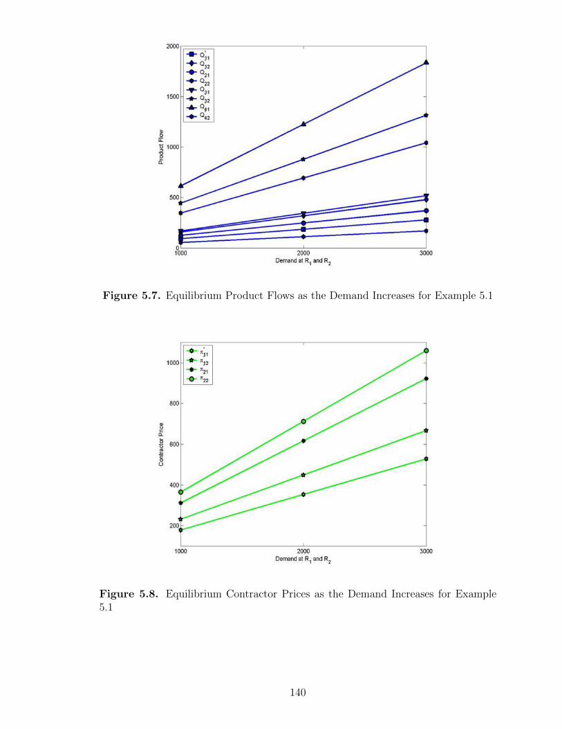
Figure 5.7. Equilibrium Product Flows as the Demand Increases for Example 5.1

Figure 5.8. Equilibrium Contractor Prices as the Demand Increases for Example5.1

140

Figure 5.9. Equilibrium Quality Levels as the Demand Increases for Example 5.1

equilibrium prices and the equilibrium quality levels in Figure 5.8 and Figure 5.9,

respectively. The contractors consistently provide the majority of the product to the

demand markets.

Observe from Figure 5.8 that as the demand increases the quality levels for both

contractors drops to zero.

Example 5.2

A disruption to the original supply chain in Example 5.1 is considered. No business is

immune from supply chain disruptions and, particularly, as noted by Purtell (2010),

pharmaceuticals are especially vulnerable since they are high-value, highly regulated

products. Moreover, pharmaceuticals disruptions may not only increase costs but

may also create hazards and expose the pharmaceutical companies to damage to

their brands and reputations (see also Nagurney, Yu, and Qiang (2011), Masoumi,

Yu, and Nagurney (2012), and Qiang and Nagurney (2012)).

141

��0Firm

��

��Firm’s Plants M1

?��R1

@@@R

��M2

?��R2

Demand Markets

��

@@@R��O1��)

��

Contractor


Specifically, I consider the following disruption. The data are as in Example 5.1

but contractor O2 is not able to provide any production and distribution services.

This could arise due to a natural disaster, adulteration in its production process,

and/or an inability to procure an ingredient. Hence, the topology of the disrupted

supply chain network is as in Figure 5.10.

The Euler method converges in 73 iterations and yields the following new equilib-

rium solution. The computed product flows are:

Q∗11 = 218.06, Q∗12 = 141.79, Q∗21 = 260.20, Q∗22 = 25.96,

Q∗31 = 521.74, Q∗32 = 332.25.

The computed quality level of the remaining contractor is:

q∗1 = 14.60,


π∗11 = 531.74, π∗12 = 176.12.

142

With the decrease in competition among the contractors, since there is now only

one, rather than two, as in Example 5.1, the quality level of contractor O1 drops, but

the prices that it charges increases. The new average quality level is q′=51.38. The

total cost of the firm is now 1,123,226.62 whereas the profit of the first contractor is

now 123,460.67, a sizable increase relative to that with competition as in Example

5.1.

Example 5.3

The data for Example 5.3 are the same as for Example 5.1, except that the opportunity

cost functions oc11, oc12, oc21, oc22 are all equal to 0.00.



Q∗11 = 451.17, Q∗12 = 396.50, Q∗21 = 548.73, Q∗22 = 103.39,

Q∗31 = 0.00, Q∗32 = 0.00, Q∗41 = 0.00, Q∗42 = 0.00.


q∗1 = 100.00, q∗2 = 100.00,


π∗11 = 3, 060.70, π∗12 = 2, 515.08, π∗21 = 3, 060.56, π∗22 = 2, 515.16.

The total cost of the firm is 2,171,693.16 and the profits of the contractors are 0.00

and 0.00. The value of q′ is 100.00.

Because the opportunity costs are all zero, in order to improve the total profit,

the contractors will charge the firm very large prices. Thus, the original firm would

rather produce by itself than outsource to the contractors.

143

One can see, from this example, that, in addition to the total revenue term, each

contractor must consider an outsourcing price related term, such as the opportunity

cost, in its objective function. Without considering such a function, the outsourcing

quantities will all be zero (cf. (5.14)), and, hence, a contractor would not secure any

contracts from the firm.

Example 5.4

The data for Example 5.4 are the same as for Example 5.1, except the opportunity

cost functions and the demand. The demand in R1 is now 700, and the demand in

R2 is 100.

The contractors’ opportunity cost functions now become:

oc11(π11) = .5(π11 − 2)2 − 15265.29, oc12(π12) = (π12 − 1)2 − 513.93,

oc21(π21) = (π21 − 1)2 − 35751.25, oc22(π22) = .5(π22 − 2)2 − 613.20.



Q∗11 = 69.12, Q∗12 = 19.65, Q∗21 = 77.99, Q∗22 = 0.00,

Q∗31 = 174.72, Q∗32 = 45.34, Q∗41 = 378.17, Q∗42 = 35.00.


q∗1 = 77.99, q∗2 = 58.68,


π∗11 = 176.73, π∗12 = 23.67, π∗21 = 190.08, π∗22 = 37.02.

144

The total cost of the firm is 204,701.28 and the profits of the contractors are: 12,366.75

and 7,614.84. The incurred opportunity costs at the equilibrium prices are all zero.

Thus, in this example, the equilibrium prices that the contractors charge the firm are

such that they are able to adequately recover their costs, and secure contracts.

The value of q′ is 72.61.


In this chapter, I developed a supply chain network game theory model, in both

equilibrium and dynamic versions, to capture contractor selection, based on the com-

petition among the contractors in the prices that they charge as well as the quality

levels of the products that they produce. I introduced a disrepute cost associated

with the average quality at the demand markets. It is assumed that the firm is

cost-minimizing whereas the contractors are profit-maximizing.

I utilized variational inequality theory for the formulation of the governing Bertrand-

Nash equilibrium conditions and then revealed interesting dynamics associated with

the evolution of the firm’s product flows, and the contractors’ prices and quality levels.

I provided stability analysis results as well as an algorithm that can be interpreted

as a discretization of the continuous-time adjustment processes. The methodological

framework was illustrated through a series of numerical examples for which I reported

the complete input and output data for transparency purposes. The numerical stud-

ies included sensitivity analysis results as well as a disruption to the supply chain

network in that a contractor is no longer available for production and distribution.

I also discussed the scenario in which the opportunity costs on the contractors’ side

are identically equal to zero and the scenario in which the opportunity costs at the

equilibrium are all zero.

145

This chapter is a contribution to the literature on outsourcing with a focus on

quality. It also is an interesting application of game theory and associated method-

ologies.

In this chapter, only a single original firm is considered, and the in-house quality

level of the single original firm is assumed to be perfect. In contrast, in the next

chapter, Chapter 6, I consider quantity and quality competition among multiple firms,

whose products are differentiated by their brands. Moreover, instead of assuming

perfect in-house quality levels, quality levels are strategic variables of the firms in

Chapter 6. Numerical examples and sensitivity analysis are also provided.

146

CHAPTER 6

A SUPPLY CHAIN NETWORK MODEL WITHPRODUCT DIFFERENTIATION, OUTSOURCING, AND

QUALITY AND PRICE COMPETITION

In this chapter, I develop a supply chain network game theory model with prod-

uct differentiation, possible outsourcing of production and distribution, quantity and

quality competition among the firms, and quality and price competition among the

contractors. The model in this chapter extends the one in Chapter 5.

This chapter, in contrast to Chapter 5, focuses on the supply chain network con-

sisting of multiple competing firms with product differentiation and their potential

contractors. For each contractor, the number of contracted original firms is not pre-

determined. In addition, unlike Chapter 5, the in-house quality levels are no longer

assumed to be perfect, and are considered as the strategic variables for the firms.

I assume that the original firms compete in the sense of Cournot-Nash. Each firm

aims at determining its equilibrium in-house quality level, in-house production quan-

tities and shipments, and outsourcing quantities, which satisfy demand requirements,

so as to minimize its total cost and the weighted cost of disrepute. The contractors,

in turn, are competing a la Bertrand-Nash in determining their optimal quality and

price levels in order to maximize their individual total profits. This model provides

each original firm with the equilibrium in-house quality level and the equilibrium

make-or-buy and contractor-selection policy, with the demand for its product being

satisfied in multiple demand markets. The demand of the product is still assumed to

be fixed in this model, as in Chapter 5.

147

In this chapter, the governing equilibrium conditions of the model are formulated

as a variational inequality problem. The Euler method (cf. Section 2.5.1), which

provides a discrete-time adjustment process and tracks the evolution of the product

flows, quality levels, and prices over time, is, again, utilized and convergence results

given. Numerical examples are provided to illustrate how such a supply chain network

game theory model can be applied in practice.

This chapter is based on Nagurney and Li (2015). It is organized as follows.

In Section 6.1, I describe the decision-making behavior of the original firms, who

compete in quantity and quality, and that of the contractors, who compete in price and

quality. Then, I construct the supply chain network game theory model with product

differentiation, possible outsourcing of production and distribution, and quality and

price competition. I obtain the governing equilibrium conditions, and derive the

equivalent variational inequality formulation. In Section 6.2, I describe the closed

form expressions yielded by the Euler method for the prices and the quality levels, with

the product flows being solved exactly by an equilibration algorithm. Convergence

results are also provided. It is applied in Section 6.3 to compute solutions to numerical

examples, along with sensitivity analysis, in order to demonstrate the generality and

the applicability of the proposed framework. In Section 6.4, I summarize the results

and present the conclusions.

6.1. The Supply Chain Network Model with Product Differ-

entiation, Outsourcing, and Quality and Price Compe-

tition

In this section, I develop the supply chain network game theory model with prod-

uct differentiation, outsourcing, price and quality competition among the contractors,

and quantity and quality competition among the original firms. I consider a finite

number of I original firms, with a typical firm denoted by i, who compete noncoopera-

148

tively. The products of the I firms are not homogeneous but, rather, are differentiated

by brands. Firm i; i = 1, . . . , I, is involved in the processes of in-house manufacturing

and distribution of its brand name product, and may subcontract its manufacturing

and distribution activities to contractors who may be located overseas. I seek to

determine the optimal product flows from each firm to its demand markets, along

with the prices the contractors charge the firms, and the quality levels of the in-house

manufactured products and the outsourced products.

For clarity and definiteness, I consider the supply chain network topology of the

I firms depicted in Figure 6.1. Each firm i; i = 1, . . . , I, is considering in-house and

outsourcing manufacturing facilities and serves the same nR demand markets. A link

from each top-tiered node i, representing original firm i, is connected to its in-house

manufacturing facility node M i. The in-house distribution activities of firm i, in turn,

are represented by links connecting M i to the demand nodes: R1, . . . , RnR .

Firm 1

1

Firm I

I��

��

M1��

O1��

· · · ��

OnO M I��

R1��

· · · ��

RnR

· · ·

?

PPPPPPPPPPPPPP

XXXXXXXXXXXXXXXXXXXXq z ?

��

��) 9

llllllllllllll

bbbbbbbbbbbbbbbbbbbb

""""""""""""""""""""

,,,,,,,,,,,,,,R� j�U

TTTTTTTTTTTT�

��

? ?� U

· · ·· · ·· · ·

In-houseManufacturing

In-houseManufacturing

In-houseDistribution

In-houseDistributionOutsourced Manufacturing

and Distribution

TransactionActivities

TransactionActivities

Figure 6.1. The Supply Chain Network Topology with Outsourcing and MultipleCompeting Firms

149

In this model, I capture the possible outsourcing of the products from the I firms

in terms of their production and delivery. As depicted in Figure 6.1, there are nO

contractors available to each of the I firms. Each firm may potentially contract to

any of these contractors who then produce and distribute the product to the same

nR demand markets. In Figure 6.1, hence, there are additional links from each top-

most node i; i = 1, . . . , I, to the nO contractor nodes, O1, . . . , OnO , each of which

corresponds to the transaction activity of firm i with contractor j. The next set of

links, which emanates from the contractor nodes to the demand markets, reflect the

production and delivery of the outsourced products to the nR demand markets.

As shown in Figure 6.1, the outsourced flows of different firms are represented by

links with different colors, for convenience and clarity of depiction, which indicates

that, in the processes of transaction and outsourcing of manufacturing and distribu-

tion, the outsourced products are still differentiated by brands. In Figure 6.1, red

links are used to denote the outsourcing flows of firm 1 with blue links referring to

those of firm I. The mathematical notation given in Table 6.1 explicitly handles such

options.

In Figure 6.1, the top set of links consists of the manufacturing links, whether

in-house or outsourcing, whereas the next set of links consists of the associated dis-

tribution links. For simplicity, let n = 1 + nO, where nO is the number of potential

contractors, denote the number of manufacturing plants, whether in-house or belong-

ing to the contractors’.

The notation for the model is given in Table 6.1. The vectors are assumed to be

column vectors. The optimal/equilibrium solution is denoted by “∗”.

For consistency, I define and quantify quality levels, quality costs, production and

delivery/transportation costs, transaction cost, and the disrepute cost in a manner

similar to that in Chapter 5. However, unlike Chapter 5, the in-house quality levels

are now strategic variables for the firms, therefore, in this model, in addition to the

150

Table 6.1. Notation for the Supply Chain Network Model with Product Differenti-ation, Outsourcing, and Quality and Price Competition

Notation DefinitionQijk the nonnegative amount of firm i’s product produced at man-

ufacturing plant j, whether in-house or contracted, and deliv-ered to demand market Rk, where j = 1, . . . , n. For firm i, itsown {Qijk} elements are grouped into the vector Qi, and allsuch vectors for all original firms are grouped into the vectorQ, where Q ∈ RInnR

+ . All in-house quantities are grouped intothe vector Q1 ∈ RInR

+ , with all outsourcing quantities into thevector Q2 ∈ RInRnO

+ .dik the demand for firm i’s product at demand market Rk; k =

1, . . . , nR.

qi the nonnegative quality level of firm i’s product produced in-house. I group the {qi} elements into the vector q1 ∈ RI

+.qij the nonnegative quality level of firm i’s product produced by

contractor j; j = 1, . . . , nO. I group all the {qij} elements forfirm i’s product into the vector q2

i ∈ RnO+ . For each contractor

j, I group its own {qij} elements into the vector qj, and thengroup all such vectors for all contractors into the vector q2 ∈RInO

+ .q All the qi and qij are grouped into the vector q ∈ RIn

+ .

πijk the price charged by contractor j; j = 1, . . . , nO, for producingand delivering a unit of firm i’s product to demand marketRk. The {πijk} elements for contractor j are grouped intothe vector πj ∈ RInR

+ , and group all such vectors for all thecontractors into the vector π ∈ RInRnO

+ .fi(Q

1, q1) the total in-house production cost of firm i.

ci(q1) the total quality cost of firm i.

tcij(∑nR

k=1 Qi,1+j,k) the total transaction cost associated with firm i transactingwith contractor j; j = 1, . . . , nO.

cik(Q1, q1) the total transportation cost associated with delivering firm

i’s product manufactured in-house to demand market Rk; k =1, . . . , nR.

scijk(Q2, q2) the total cost of contractor j; j = 1, . . . , nO, to produce and

distribute the product of firm i to demand market Rk.cj(q

2) the total quality cost faced by contractor j; j = 1, . . . , nO.

ocijk(π) the opportunity cost associated with pricing the product offirm i at πijk, and delivering to demand market Rk, by con-tractor j; j = 1, . . . , nO.

q′i(Qi, qi, q2i ) the average quality level of firm i’s product (cf. (6.3)).

dci(q′i(Qi, qi, q

2i )) the cost of disrepute of firm i.

151

outsourcing production and distribution costs, I also express the in-house production

and distribution costs as functions that depend on both production quantities and

quality levels. These functions are assumed to be convex in quality and quantity.

6.1.1 The Behavior of the Firms and Their Optimality Conditions

Unlike Chapter 5, the in-house quality levels are not assumed to be perfect any-

more. As mentioned in Table 6.1, the quality level of firm i’s product produced

in-house is denoted by qi, where i = 1, . . . , I, and the quality level of firm i’s product

produced by contractor j is denoted by qij, where j = 1, . . . , nO. Both vary from a 0%

conformance level to a 100% conformance level (cf. Section 1.1), so that, respectively,

0 ≤ qij ≤ qU , i = 1, . . . , I; j = 1, . . . , nO, (6.1)

0 ≤ qi ≤ qU , i = 1, . . . , I, (6.2)

where qU is the value representing perfect quality level associated with the 100%

conformance level.

The average quality level of firm i’s product is, hence, an average quality level

determined by the in-house quality level, the in-house product flows, the quality

levels of the contractors, and the outsourced product flows. Thus, the average quality

level for firm i’s product, both in-house and outsourced, can be expressed as

q′i(Qi, qi, q2i ) =

∑nRk=1

∑nj=2Qijkqi,j−1 +

∑nRk=1Qi1kqi∑nR

k=1 dik, i = 1, . . . , I. (6.3)

Compared to the average quality levels in Chapters 3 (cf. (3.7)) and 5 (cf. (5.2)), (6.3)

captures the average quality levels at the demand markets in a competitive supply

chain network with product differentiation and outsourcing.

Following Chapter 5, I assume that the disrepute cost of firm i, dci(q′i(Qi, qi, q

2i )),

is a monotonically decreasing function of the average quality level. Here, however, I

152

no longer assume, as was done in Chapter 5, which considered only a single firm, that

the firms produce their branded products with perfect quality. Hence, the average

quality level in (6.3) is a generalization of (5.2).

Each original firm i selects the product flows Qi and the in-house quality level qi,

whereas each contractor j, who competes for contracts in quality and price, selects

its outsourcing quality level vector qj and outsourcing price vector πj.

Firm i’s utility function is denoted by U1i , where i = 1, . . . , I. The objective of

original firm i is to maximize its utility (cf. (6.4) below) represented by minus its

total costs that include the production cost, the quality cost, the transportation costs,

the payments to the contractors, the transaction costs, along with the weighted cost

of disrepute, with the nonnegative term ωi denoting the weight that firm i imposes

on the disrepute cost function (cf. Section 2.4).

As discussed in Chapter 5, the production and transportation cost functions only

capture the costs of production and delivery, and depend on both the quantities and

the quality levels. The production and the transportation costs and the quality cost

are entirely different costs, and they do not overlap.

Hence, firm i seeks to

MaximizeQi,qi U1i = −fi(Q1, q1)− ci(q1)−

nR∑k=1

cik(Q1, q1)−

nO∑j=1

nR∑k=1

π∗ijkQi,1+j,k

−nO∑j=1

tcij(

nR∑k=1

Qi,1+j,k)− ωidci(q′i(Qi, qi, q2∗

i )) (6.4)

subject to:n∑j=1

Qijk = dik, i = 1, . . . , I; k = 1, . . . , nR, (6.5)

Qijk ≥ 0, i = 1, . . . , I; j = 1, . . . , n; k = 1, . . . , nR, (6.6)

and (6.2).

153

As revealed by constraint (6.5), a fixed demand is assumed for each firm, in order

to capture the forecasted/projected demands at multiple demand markets. Note that,

according to (6.4), the prices and the contractors’ quality levels are evaluated at their

equilibrium values.

I assume that all the cost functions in (6.4) are continuous, twice continuously

differentiable, and convex. The original firms compete in a noncooperative in the

sense of Nash with each one trying to maximize its own utility. The strategic variables

for each original firm i are all the in-house and the outsourcing flows produced and

shipped by firm i and its in-house quality level.

I define the feasible set Ki as Ki = {(Qi, qi)|Qi ∈ RnnR+ with (6.5) satisfied and qi

satisfying (6.2)}. All Ki; i = 1, . . . , I, are closed and convex. I also define the feasible

set K1 ≡ ΠIi=1Ki.

Definition 6.1: Supply Chain Network Cournot-Nash Equilibrium with

Product Differentiation, Outsourcing, and Quality Competition

An in-house and outsourced product flow pattern and in-house quality level (Q∗, q1∗)

∈ K1 is said to constitute a Cournot-Nash equilibrium if for each firm i; i = 1, . . . , I,

U1i (Q∗i , Q

∗i , q∗i , q∗i , q

2∗, π∗i ) ≥ U1i (Qi, Q

∗i , qi, q

∗i , q

2∗, π∗i ), ∀(Qi, qi) ∈ Ki, (6.7)

where

Q∗i ≡ (Q∗1, . . . , Q∗i−1, Q

∗i+1, . . . , Q

∗I),

q∗i ≡ (q∗1, . . . , q∗i−1, q

∗i+1, . . . , q

∗I ).

According to (6.7) (cf. Definition 2.7), a Cournot-Nash equilibrium is established

if no firm can unilaterally improve upon its utility by selecting an alternative vector

of in-house or outsourced product flows and quality level.

154

Next, I derive the variational inequality formulation of the Cournot-Nash equi-

librium with product differentiation and outsourcing according to Definition 6.1 (cf.

Cournot (1838), Nash (1950, 1951), Gabay and Moulin (1980), and Theorem 2.7) in

the following theorem.

Theorem 6.1

Assume that, for each firm i; i = 1, . . . , I, the utility function U1i (Q, q1, q2∗, π∗i ) is

concave with respect to its variables Qi and qi, and is continuous and twice continu-

ously differentiable. Then (Q∗, q1∗) ∈ K1 is a Counot-Nash equilibrium according to

Definition 6.1 if and only if it satisfies the variational inequality:

−I∑i=1

n∑h=1

nR∑m=1

∂U1i (Q∗, q1∗ , q2∗ , π∗i )

∂Qihm

× (Qihm −Q∗ihm)

−I∑i=1

∂U1i (Q∗, q1∗q2∗ , π∗i )

∂qi× (qi − q∗i ) ≥ 0,

∀(Q, q1) ∈ K1, (6.8)

with notice that: for h = 1; i = 1, . . . , I; m = 1, . . . , nR:

− ∂U1i

∂Qihm

=

[∂fi

∂Qihm

+

nR∑k=1

∂cik∂Qihm

+ ωi∂dci∂q′i

∂q′i∂Qihm

],

for h = 2, . . . , n; i = 1, . . . , I; m = 1, . . . , nR:

− ∂U1i

∂Qihm

=

[π∗i,h−1,m +

∂tci,h−1

∂Qihm

+ ωi∂dci∂q′i

∂q′i∂Qihm

],

for i = 1, . . . , I:

−∂U1i

∂qi=

[∂fi∂qi

+∂ci∂qi

+

nR∑k=1

∂cik∂qi

+ ωi∂dci∂q′i

∂q′i∂qi

].

155

6.1.2 The Behavior of the Contractors and Their Optimality Conditions

The objective of contractor j; j = 1, . . . , nO, is profit maximization. Their rev-

enues are obtained from the purchasing activities of the original firms, while their

costs are the costs of production and distribution, the total quality costs, and the

opportunity costs (cf. Section 5.1.2).

Similar as in Chapter 5, in this model, each contractor has, as its strategic vari-

ables, its quality levels for producing and distributing the original firms’ products,

and the prices that charges the firms. I denote the utility of each contractor j by U2j ,

with j = 1, . . . , nO, and note that it represents the profit. Hence, each contractor j;

j = 1, . . . , nO, seeks to:

Maximizeqj ,πj U2j =

nR∑k=1

I∑i=1

πijkQ∗i,1+j,k −

nR∑k=1

I∑i=1

scijk(Q2∗, q2)− cj(q2)

−nR∑k=1

I∑i=1

ocijk(π) (6.9)

subject to:

πijk ≥ 0, j = 1, . . . , nO; k = 1, . . . , nR, (6.10)

and (6.1) for each j. are at their equilibrium values.

According to (6.9), the original firms’ outputs are evaluated at the equilibrium,

since the contractors do not control these variables, and, hence, must respond to these

outputs.

The cost functions in each contractor’s utility function are continuous, twice con-

tinuously differentiable, and convex. The contractors compete in a noncooperative in

the sense of Nash, with each one trying to maximize its own profits.

The feasible sets are defined as Kj ≡ {(qj, πj)|qj satisfies (6.1) and πj satisfies (6.

10) for j}, K2 ≡ ΠnOj=1Kj, and K ≡ K1 × K2. All the above-defined feasible sets are

convex.

156

Definition 6.2: A Bertrand-Nash Equilibrium with Price and Quality Com-

petition

A quality level and price pattern (q2∗, π∗) ∈ K2 is said to constitute a Bertrand-Nash

equilibrium if for each contractor j; j = 1, . . . , nO,

U2j (Q2∗ , q∗j , q

∗j , π

∗j , π

∗j ) ≥ U2

j (Q2∗ , qj, q∗j , πj, π

∗j ), ∀(qj, πj) ∈ Kj, (6.11)

where

q∗j ≡ (q∗1, . . . , q∗j−1, q

∗j+1, . . . , q

∗nO

),

π∗j ≡ (π∗1, . . . , π∗j−1, π

∗j+1, . . . , π

∗nO

).


if no contractor can unilaterally improve upon its profits by selecting an alternative

vector of quality levels or prices charged to the original firms.

I present the variational inequality formulation of the Bertrand-Nash equilibrium

according to Definition 6.2 (see, Bertrand (1883), Nash (1950, 1951), Gabay and

Moulin (1980), and Theorem 2.7) in the following theorem.

Theorem 6.2

Assume that, for each contractor j; j = 1, . . . , nO, the profit function U2j (Q2∗ , q2, π)

is concave with respect to the variables πj and qj, and is continuous and twice contin-

uously differentiable. Then (q2∗, π∗) ∈ K2 is a Bertrand-Nash equilibrium according

to Definition 6.2 if and only if it satisfies the variational inequality:

−I∑l=1

nO∑j=1

∂U2j (Q2∗ , q2∗ , π∗)

∂qlj× (qlj − q∗lj)

−I∑l=1

nO∑j=1

nR∑k=1

∂U2j (Q2∗ , q2∗ , π∗)

∂πljk× (πljk − π∗ljk) ≥ 0,

157

∀(q2, π) ∈ K2. (6.12)

with notice that: for j = 1, . . . , nO; l = 1, . . . , I:

−∂U2

j

∂qlj=

I∑i=1

nR∑k=1

∂scijk∂qlj

+∂cj∂qlj

,

and for j = 1, . . . , nO; l = 1, . . . , I; k = 1, . . . , nR:

−∂U2

j

∂πljk=

I∑i=1

nR∑r=1

∂ocijr∂πljk

−Q∗l,1+j,k.


Product Differentiation, Outsourcing, and Quality and Price Com-

petition

In equilibrium, the optimality conditions for all contractors and the optimality

conditions for all the original firms must hold simultaneously, according to the defi-

nition below.

Definition 6.3: Supply Chain Network Equilibrium with Product Differ-

entiation, Outsourcing, and Quality and Price Competition

The equilibrium state of the supply chain network with product differentiation, out-

sourcing, and quality and price competition is one where both variational inequalities

(6.8) and (6.12) hold simultaneously.

Theorem 6.3

The equilibrium conditions governing the supply chain network model with product

158

differentiation, outsourcing, and quality competition are equivalent to the solution of

the variational inequality problem: determine (Q∗, q1∗ , q2∗ , π∗) ∈ K, such that:

−I∑i=1

n∑h=1

nR∑m=1

∂U1i (Q∗, q1∗ , q2∗ , π∗i )

∂Qihm

×(Qihm−Q∗ihm)−I∑i=1

∂U1i (Q∗, q1∗ , q2∗ , π∗i )

∂qi×(qi−q∗i )

−I∑l=1

nO∑j=1

∂U2j (Q2∗ , q2∗ , π∗)

∂qlj× (qlj − q∗lj)

−I∑l=1

nO∑j=1

nR∑k=1

∂U2j (Q2∗ , q2∗, π∗)

∂πljk× (πljk − π∗ljk) ≥ 0,

∀(Q, q1, q2, π) ∈ K. (6.13)

Proof: The proof follows a manner similar to that for Theorem 5.3.�

Variational inequality (6.13) can be put into standard form (cf. (2.1a)): determine

X∗ ∈ K such that:

〈F (X∗), X −X∗〉 ≥ 0, ∀X ∈ K, (6.14)

where 〈·, ·〉 denotes the inner product in N -dimensional Euclidean space, and N =

InnR + I + InO + InOnR. If the column vectors X ≡ (Q, q1, q2, π) and F (X) ≡

(F1(X), F2(X), F3(X), F4(X)), such that:

F1(X) =

[∂U1

i (Q, q1, q2, πi)

∂Qihm

; h = 1, . . . , n; i = 1, . . . , I;m = 1, . . . , nR

],

F2(X) =

[∂U1

i (Q, q1, q2, πi)

∂qi; i = 1, . . . , I

],

F3(X) =

[∂U2

j (Q2, q2, π)

∂qlj; l = 1, . . . , I; j = 1, . . . , nO

],

F4(X) =

[∂U2

j (Q2, q2, π)

∂πljk; l = 1, . . . , I; j = 1, . . . , nO; k = 1, . . . , nR

], (6.15)

then (6.13) can be re-expressed as (2.1a).

159


Supply Chain Network with Product Differentiation, Out-

sourcing, and Quality and Price Competition

The algorithm employed for the computation of the solution for the supply chain

network game theory model is the Euler method (cf. Section 2.5.1).

Similar to the discussion in Chapter 5 (cf. (5.3)), at each iteration τ , the values of

the product flows can be determined by the exact equilibration algorithm of Dafermos

and Sparrow (1969) (cf. Sections 2.5.1 and 5.3). Furthermore, one can determine the

values for the in-house and the outsourced quality variables explicitly according to

the following closed form expressions: for each original firm i; i = 1, . . . , I:

qτ+1i = min{qU ,max{0, qτi − aτ (

∂fi(Q1τ , q1τ )

∂qi+∂ci(q

1τ )

∂qi+

nR∑k=1

∂cik(Q1τ , q1τ )

∂qi

+ωi∂dci(q

′iτ )

∂q′i

∂q′i(Qτi , q

τi , q

2τ

i )

∂qi)}}; (6.16)

and for the contractor and firm pairs: l = 1, . . . , I; j = 1, . . . , nO:

qτ+1lj = min{qU ,max{0, qτlj − aτ (

I∑i=1

nR∑k=1

∂scijk(Q2τ , q2τ )

∂qlj+∂cj(q

2τ )

∂qlj)}}. (6.17)

Also, the following are the explicit formulae for the outsourced product prices: for

l = 1, . . . , I; j = 1, . . . , nO; k = 1, . . . , nR:

πτ+1ljk = max{0, πτljk − aτ (

I∑i=1

nR∑r=1

∂ocijr(πτ )

∂πljk−Qτ

l,1+j,k)}. (6.18)

I now provide the convergence result. The proof follows using similar arguments

as those in Theorem 2.17 and Nagurney and Zhang (1996).

160

Theorem 6.4

In the supply chain network game theory model with product differentiation, out-

sourcing, and quality competition, let F (X) = −∇U(Q, q1, q2, π), where I group all

U1i ; i = 1, . . . , I, and U2

j ; j = 1, . . . , nO, into the vector U(Q, q1, q2, π), be strongly

monotone. Also, assume that F is uniformly Lipschitz continuous (cf. Definition

2.6). Then there exists a unique equilibrium product flow, quality level, and price pat-

tern (Q∗, q1∗ , q2∗ , π∗) ∈ K, and any sequence generated by the Euler method as given

by (2.34), where {aτ} satisfies∑∞

τ=0 aτ = ∞, aτ > 0, aτ → 0, as τ → ∞ converges

to (Q∗, q1∗ , q2∗ , π∗).

As discussed in Section 5.3, one can also expect the existence of a solution, given

the continuity of the functions that make up F (X), under less restrictive conditions

that that of strong monotonicity.

The Euler method (cf. (5.19) and (6.16)-(6.18)), can be interpreted as a discrete-

time adjustment process in which each iteration reflects a time step (cf. Section

2.5.1). The original firms determine, at each time step, their optimal production

(and shipment) outputs and quality levels, whereas the contractors, at each time

step (iteration), compute their optimal quality levels and the prices that they charge.

The process evolves over time until the equilibrium product flows, quality levels, and

contractor prices are achieved, at which point no one has any incentive to switch their

strategies.


In this section, I present numerical supply chain network examples for which I

applied the Euler method (cf. (5.19) and (6.16)-(6.18)) to compute the equilibrium

solutions. I present a spectrum of examples, accompanied by sensitivity analysis.

The supply chain network topology of the numerical examples is given in Figure

6.2. There are two original firms, both of which are located in North America. Their

161

products are substitutes but are differentiated by brands in the two demand markets,

R1 and R2. Demand market R1 is in North America, whereas demand market R2

is in Asia. I use different colors to denote the outsourcing links of different original

firms, with red links denoting the outsourcing links of firm 1 and blue links denoting

those of firm 2.

1 2� ��

M1� �� O1� �� O2 M2� ��

R1� �� R2

?

PPPPPPPPPP

XXXXXXXXXXXXXXq z ?

��

��) 9

llllllllll

bbbbbbbbbbbbbb

""""""""""""""

,,,,,,,,,,RU� �Rj�U

TTTTTTTTT�

��

? ?� U

Figure 6.2. The Supply Chain Network Topology for the Numerical Examples

Each original firm has one in-house manufacturing plant and two potential con-

tractors. Contractor 1 and contractor 2 are located in North America and Asia,

respectively. Each firm must satisfy the demands for its product at the two demand

markets. The demands for firm 1’s product at R1 and at R2 are 50 and 100, respec-

tively. The demands for firm 2’s product at R1 and at R2 are 75 and 150.

For the computation of solutions to the numerical examples, I implemented the

Euler method using Matlab on a Lenovo Z580. The convergence tolerance is 10−6,

so that the algorithm is deemed to have converged when the absolute value of the

difference between each successive product flow, quality level, and price is less than

or equal to 10−6. The sequence {aτ} is set to: {1, 12, 1

2, 1

3, 1

3, 1

3, . . .}. I initialized the

algorithm by equally distributing the product flows among the paths joining the firm

162

top-node to the demand market, by setting the quality levels equal to 1 and the prices

equal to 0.

Example 6.1

The data are as follows.

The production cost functions at the in-house manufacturing plants are:

f1(Q1, q1) = (Q111 +Q112)2 + 1.5(Q111 +Q112) + 2(Q211 +Q212) + .2q1(Q111 +Q112),

f2(Q1, q1) = 2(Q211 +Q212)2 + .5(Q211 +Q212) + (Q111 +Q112) + .1q2(Q211 +Q212).

The total transportation cost functions for the in-house manufactured products

are:

c11(Q111) = Q2111 + 5Q111, c12(Q112) = 2.5Q2

112 + 10Q112,

c21(Q211) = .5Q2211 + 3Q211, c22(Q212) = 2Q2

212 + 5Q212.

The in-house total quality cost functions for the two original firms are given by:

c1(q1) = (q1 − 80)2 + 10, c2(q2) = (q2 − 85)2 + 20.

The transaction cost functions are:

tc11(Q121 +Q122) = .5(Q121 +Q122)2 + 2(Q121 +Q122) + 100,

tc12(Q131 +Q132) = .7(Q131 +Q132)2 + .5(Q131 +Q132) + 150,

tc21(Q221 +Q222) = .5(Q221 +Q222)2 + 3(Q221 +Q222) + 75,

tc22(Q221 +Q222) = .75(Q231 +Q232)2 + .5(Q231 +Q232) + 100.

The contractors’ total cost functions of production and distribution are:

sc111(Q121, q11) = .5Q121q11, sc112(Q122, q11) = .5Q122q11,

163

sc121(Q131, q12) = .5Q131q12, sc122(Q132, q12) = .5Q132q12,

sc211(Q221, q21) = .3Q221q21, sc212(Q222, q21) = .3Q222q21,

sc221(Q231, q22) = .25Q231q22, sc222(Q232, q22) = .25Q232q22.

The total quality cost functions of the contractors are:

c1(q11, q21) = (q11 − 75)2 + (q21 − 75)2 + 15,

c2(q12, q22) = 1.5(q12 − 75)2 + 1.5(q22 − 75)2 + 20.

The contractors’ opportunity cost functions are:

oc111(π111) = (π111 − 10)2, oc121(π121) = .5(π121 − 5)2,

oc112(π112) = .5(π112 − 5)2, oc122(π122) = (π122 − 15)2,

oc211(π211) = 2(π211 − 20)2, oc221(π221) = .5(π221 − 5)2,

oc212(π212) = .5(π212 − 5)2, oc222(π222) = (π222 − 15)2.

The original firms’ disrepute cost functions are:

dc1(q′1) = 100− q′1, dc2(q′2) = 100− q′2,

where

q′1 =Q121q11 +Q131q12 +Q111q1 +Q122q11 +Q132q12 +Q112q1

d11 + d12

,

and

q′2 =Q221q21 +Q231q22 +Q211q2 +Q222q21 +Q232q22 +Q212q2

d21 + d22

.

ω1 and ω2 are 1. qU is 100.


solution.

164

The computed product flows are:

Q∗111 = 13.64, Q∗121 = 26.87, Q∗131 = 9.49, Q∗112 = 9.34, Q∗122 = 42.85,

Q∗132 = 47.81, Q∗211 = 16.54, Q∗221 = 47.31, Q∗231 = 11.16, Q∗212 = 12.65,

Q∗222 = 62.90, Q∗232 = 74.45.

The computed quality levels of the original firms and the contractors are:

q∗1 = 77.78, q∗2 = 83.61, q∗11 = 57.57, q∗12 = 65.45, q∗21 = 58.47, q∗22 = 67.87.

The equilibrium prices are:

π∗111 = 23.44, π∗112 = 47.85, π∗121 = 14.49, π∗122 = 38.91,

π∗211 = 31.83, π∗212 = 67.90, π∗221 = 16.16, π∗222 = 52.23.

Notice that, although the North American contractor produces at a lower qual-

ity and at a higher price at equilibrium, it produces and distributes more than the

off-shore contractor to R1, who is located in North America. This happens for two

reasons. First, because of the fixed demands, no pressure for quality improvement is

imposed from the demand side. Secondly, as reflected in the transaction costs with

the North America contractor, firms are willing to outsource more to this contractor.

The Asian contractor, who produces at higher quality levels and at lower prices at

equilibrium, produces and distributes more to R2. This happens because the contrac-

tor who charges lower prices and produces at higher quality levels is highly preferable

in the demand market, R2, with the larger demand for which the original firms need

to outsource more.

165

The total costs of the original firms’ are, respectively, 11,419.90 and 24,573.94,

with their incurred disrepute costs being 36.32 and 34.69. The profits of the con-

tractors are 567.84 and 440.92. The values of q′1 and q′2 are, respectively, 63.68 and

65.31.

I now conduct sensitivity analysis by varying the weights that the firms im-

pose on their disrepute costs, ω, which is the vector of ωi; i = 1, 2, with ω =

(0, 0), (1000, 1000), (2000, 2000), (3000, 3000), (4000, 4000), (5000, 5000).

I display the equilibrium product flows and the equilibrium quality levels, both

the in-house and the outsourced ones, and the average quality levels, in Figure 6.3,

with the equilibrium prices changed by each contractor, the disrepute cost, and the

total cost of each original firm displayed in Figure 6.4.

As the weights of the disrepute costs increase, there is more pressure for firms to

improve quality. Thus, all the quality levels increase. In addition, because the in-

house activities are more capable of guaranteeing higher quality, the outputs of both

firms are shifted in-house as the weights increase. As a result, the outsourcing prices

decrease (see (6.12)). Moreover, as shown in Figure 6.4, as expected, the values of

the incurred disrepute costs decrease as ω increases, but the total costs of the original

firms increase.

Example 6.2

In Example 6.2, both firms consider quality levels as variables affecting their in-house

transportation costs. The transportation cost functions of the original firms, hence,

now depend on in-house quality levels as follows:

c11(Q111, q1) = Q2111 + 1.5Q111q1, c12(Q112, q1) = 2.5Q2

112 + 2Q112q1,

c21(Q211, q2) = .5Q2211 + 3Q211q2, c22(Q212, q2) = 2Q2

212 + 2Q212q2.

The remaining data are identical to those in Example 6.1.

166

Figure 6.3. Equilibrium Product Flows and Quality Levels as ω Increases for Ex-ample 6.1

167

Figure 6.4. Equilibrium Prices, Disrepute Costs, and Total Costs of the Firms as ωIncreases for Example 6.1


solution.

The computed product flows are:

Q∗111 = 0.00, Q∗121 = 36.42, Q∗131 = 13.58, Q∗112 = 0.00, Q∗122 = 46.42,

Q∗132 = 53.58, Q∗211 = 0.00, Q∗221 = 60.13, Q∗231 = 14.87, Q∗212 = 3.83,

Q∗222 = 65.50, Q∗232 = 80.68.

168

The computed quality levels of the original firms and the contractors are:

q∗1 = 80, q∗2 = 80.90, q∗11 = 54.29, q∗12 = 63.81, q∗21 = 56.16, q∗22 = 67.04.

The equilibrium prices are:

π∗111 = 28.21, π∗112 = 51.42, π∗121 = 18.58, π∗122 = 41.79,

π∗211 = 35.03, π∗212 = 70.50, π∗221 = 19.87, π∗222 = 55.34.

The total costs of the original firms are, respectively, 13,002.64 and 27,607.44,

with incurred disrepute costs of 41.45 and 38.80. The profits of the contractors are,

respectively, 967.96 and 656.78. The average quality levels of the original firms, q′1

and q′2, are 58.55 and 61.20.

I also conduct sensitivity analysis by varying the weights associated with the disre-

pute costs, ω, for ω = (0, 0), (1000, 1000), (2000, 2000), (3000, 3000), (4000, 4000), (5000,

5000). The results of this sensitivity analysis are displayed in Figures 6.5 and 6.6.

I now discuss the results of the sensitivity analysis for Example 6.2. As shown

in Figures 6.5 and 6.6, as the weights of the disrepute costs increase, the changing

trends of all the variables and costs in Figures 6.5 and 6.6 are the same as those in

Example 6.1, except the trends for Q∗231, q∗22, and π∗221. As ω increases from 0 to 2000,

Q∗231 increases. However, as ω increases further, Q∗231 decreases. The trends of q∗22

and π∗221 then change accordingly.

The reason is as follows. Because now in-house transportation costs more than

before, in order to satisfy the fixed demand d21, firm 2 tends to shift more production

and distribution to the contractor with a good quality level, when ω is small. This

is why Q∗231 increases as ω increases from 0 to 2000. Nevertheless, as ω increases

further, firm 2 is under greater pressure to improve quality. Therefore, firm 2 then

shifts more production in-house, and, as a result, Q∗231 decreases.

169

Figure 6.5. Equilibrium Product Flows and Quality Levels as ω Increases for Ex-ample 6.2

170

Figure 6.6. Equilibrium Prices, Disrepute Costs, and Total Costs of the Firms as ωIncreases for Example 6.2

For firm 1, whose cost functions are completely distinct from those of firm 2, it

is always more cost-wise for it to improve quality by shifting product flows in-house.

Thus, the changing trends of all the variables and costs of firm 1 in Figures 6.5 and

6.6 are either monotonically increasing or decreasing.

I now compare Examples 6.1 and 6.2 with ω in both examples equal to 0. Please

refer to the preceding figures. This case is interesting and informative since it repre-

sents the scenario that neither firm 1 nor firm 2 cares about its possible reputation

171

loss due to its product/brand having a lower quality. After the incorporation of qual-

ity levels into both firms’ in-house transportation costs, it now costs more for both

firms to transport the same amounts of their products manufactured in-house and

to maintain the same in-house quality levels as in Example 6.1, as reflected by the

in-house transportation functions in Examples 6.1 and 6.2. Thus, in Example 6.2,

the equilibrium in-house product flows are lower as compared to those in Example

6.1, and, in order to satisfy the demands, the equilibrium outsourced flows of both

firms are higher. The corresponding results are: the contractors charge more to the

firms; the outsourcing quality levels of the contractors are lower; the contractors’ total

profits increase, and the firms’ total costs are higher than those in Example 6.1.

Example 6.3

In Example 6.3, I consider the scenario that the in-house transportation from the

two firms to each demand market gets much more congested than before, and each

firm’s in-house quantities also affect the other firm’s in-house transportation costs.

The total in-house transportation cost functions of the two firms now become:

c11(Q111, Q211, q1) = Q2111 + 1.5Q111q1 + 7Q211,

c12(Q112, Q212.q1) = 2.5Q2112 + 2Q112q1 + 10Q212,

c21(Q211, Q111, q2) = .5Q2211 + 3Q211q2 + 8Q111,

c22(Q212, Q112, q2) = 2Q2212 + 2Q212q2 + 10Q112.

The remaining data are identical to those in Example 6.1.

The total costs of firm 1 and firm 2 associated with different ω values are displayed

in Tables 6.2 and 6.3, respectively. Note that, in Table 6.2, the total cost of firm 1

increases monotonically, whether ω1 or ω2 increases. The same result is inferred from

Table 6.3 for firm 2.

172

Table 6.2. Total Costs of Firm 1 with Different Sets of ω1 and ω2

ω ω1 = 0 ω1 = 1000 ω1 = 2000 ω1 = 3000 ω1 = 4000 ω1 = 5000

ω2 = 0 12,999.09 45,135.09 61,322.22 71,463.36 77,437.89 80,462.63ω2 = 1000 13,218.71 45,348.05 61,535.18 71,676.32 77,650.85 80,675.60ω2 = 2000 13,425.67 45,571.40 61,758.53 71,899.67 77,874.20 80,898.94ω2 = 3000 13,666.29 45,812.52 61,999.65 72,140.79 78,115.32 81,114.01ω2 = 4000 14,091.85 46,034.08 62,221.20 72,362.34 78,336.88 81,361.62ω2 = 5000 14,091.85 46,239.00 62,426.12 72,567.26 78,541.80 81,566.54

Table 6.3. Total Costs of Firm 2 with Different Sets of ω1 and ω2

ω ω1 = 0 ω1 = 1000 ω1 = 2000 ω1 = 3000 ω1 = 4000 ω1 = 5000

ω2 = 0 27,585.65 28,203.96 28,561.15 28,798.10 29,005.24 29,187.92ω2 = 1000 62,896.33 63,626.00 63,983.19 64,220.14 64,427.28 64,609.96ω2 = 2000 92,753.88 93,312.11 93,669.30 93,906.25 94,113.39 94,296.07ω2 = 3000 116,378.40 116,981.94 117,339.13 117,576.08 117,783.22 117,965.90ω2 = 4000 135,237.43 135,872.91 136,230.10 136,467.05 136,674.19 136,856.87ω2 = 5000 150,231.01 150,886.51 151,243.69 151,480.65 151,687.79 151,870.47

The reason is the following. As discussed for Examples 6.1 and 6.2, when ωi; i =

1, 2, increases, the in-house production quantities of firm i increase. Now, in Example

6.3, because of the in-house production costs (as in Example 6.1) and the new in-house

transportation costs, the increase of firm i’s in-house quantities would also increase

the other firm’s total cost.

According to the results in Tables 6.2 and 6.3, strategically, if a firm has to increase

the weight of its own disrepute cost, it is more cost-wise to increase it before the other

firm does. If the firm increases its weight at the same time as, or after the other firm

does, it would incur more cost under the same disrepute cost weight.


In this chapter, I developed a supply chain network game theory model with prod-

uct differentiation, outsourcing, and price and quality competition. The original firms

compete with one another in in-house quality levels and in-house and outsouced pro-

173

duction (and shipment) flows in order to minimize their total costs and the weighted

disrepute costs. The contractors, in turn, compete in their quality levels and the prices

that they charge the original firms for manufacturing and distributing the products

to the demand markets. This model provides the optimal make-or-buy as well as

contractor selection decisions for each original firm.

I modeled the impact of quality on in-house and outsourced production and trans-

portation and on the reputation of each firm through the quantification of the quality

levels, quality cost, and the disrepute cost, with the production and the transportation

cost functions depending on both quantities and quality levels.

Variational inequality theory was employed in the formulations of the equilibrium

conditions of the original firms, the contractors, and the supply chain network game

theory model with product differentiation, possible outsourcing of production and

distribution, and quality and price competition. The algorithm adopted was the Euler

method, which provides a discrete-time adjustment process and tracks the evolution

of the in-house and outsourced production (and shipment) flows, the in-house and the

outsourced quality levels, and the prices over time. It also yields closed form explicit

formulae at each iteration with nice features for computation for all variables except

for the production/shipment ones, which are computed via an exact equilibration

algorithm.

In order to demonstrate the generality of the model and the computational scheme,

I provided solutions to a series of numerical examples, accompanied by sensitivity

analysis.

Unlike this chapter, in the next chapter, Chapter 6, a multitiered supply chain

network model with suppliers’ quality is developed. Different from contractors, which

produce and deliver products for firms, suppliers provide firms with the components

needed to assemble their products. In Chapter 6, I include the quality of suppliers and

firms in producing the components in the model. The preservation/decay of quality

174

in the assembly process of each firm is also considered and modeled as a decision

variable. Numerical examples along with sensitivity analysis are provided.

175

CHAPTER 7

A SUPPLY CHAIN NETWORK MODEL WITHSUPPLIER SELECTION AND QUALITY AND PRICE

COMPETITION

This chapter, unlike Chapters 5 and 6, focuses on the supply chain network prob-

lem with multiple competing firms and their potential suppliers. The competitive

behavior of each tier of decision-makers in the supply chain network is described

along with their strategic variables, which include quality of the components and, in

the case of the firms, the quality of the assembly process itself.

Specifically, the potential suppliers may either provide distinct components to the

firms, or provide the same component, in which case, they compete noncooperatively

with one another in terms of quality and prices. The firms, in turn, are responsible

for assembling the products under their brand names using the components needed

and transporting the products to multiple demand markets. They also have the op-

tion of producing their own components, if necessary. The firms compete in product

quantities, the quality preservation levels of their assembly processes, the contracted

component quantities produced by the suppliers, and in in-house component quan-

tities and quality levels. Each of the firms aims to maximize profits. The quality of

an end product is determined by the qualities and quality levels of its components,

produced both by the firms and the suppliers, the importance of the quality of each

component to that of the end product, and the quality preservation level of its as-

sembly process. Consumers at the demand markets respond to both the prices and

the quality of the end products. In addition, in this chapter, I provide a formula to

176

quantify the quality of the finished product based on the quality of the individual

components.

The governing equilibrium conditions of the supply chain network are formulated

as a variational inequality problem and qualitative properties are presented. The

algorithm, which is the modified projection method (cf. Section 2.5.2), accompanied

with convergence results, is then applied to numerical supply chain network exam-

ples, along with sensitivity analysis in which the impacts of capacity disruptions and

complete supplier elimination are investigated.

This chapter is based on Li and Nagurney (2015). It is organized as follows. In

Section 7.1, I develop the multitiered supply chain network model with competing

suppliers and competing firms. The variational inequality formulations for each tier

followed by a unified variational inequality are derived. In Section 7.2, the qualitative

properties of the equilibrium pattern, in particular, existence and uniqueness results,

are presented. In Section 7.3, the explicit formulae for the computation of this sup-

ply chain network problem, which is solved by the modified projection method (cf.

Section 2.5.2), are presented, along with conditions for convergence, which is then

applied in Section 7.4 to compute solutions to numerical supply chain network ex-

amples accompanied by sensitivity analysis. I summarize the results and present the

conclusions in Section 7.5.

7.1. The Supply Chain Network Model with Supplier Selec-

tion and Quality and Price Competition

In this section, I develop a multitiered supply chain network game theory model

with suppliers and firms that procure components from the suppliers for their prod-

ucts, which are differentiated by brand. I consider a supply chain network consisting

of I firms, with a typical firm denoted by i, nS suppliers, with a typical supplier de-

177

noted by j, and a total of nR demand markets, with a typical demand market denoted

by Rk.

The firms compete noncooperatively, and each firm corresponds to an individual

brand representing the product that it produces. Product i, which is the product

produced by firm i, requires nli different components, and the total number of different

components required by the I products is nl. Each supplier may be able to produce

a variety of components for each firm.

The I firms are involved in the processes of assembling the products using the

components needed, transporting the products to the demand markets, and, possibly,

producing the components of the products. The suppliers, in turn, are involved in the

processes of producing and delivering the components of the products to the firms.

Both in-house and contracted component production activities are captured in the

model. Firms’ and suppliers’ production capacities/abilities are also considered.

The network topology of the problem is depicted in Figure 7.1. The first two

sets of links from the top are links corresponding to distinct supplier components.

The links from the top-tiered nodes j; j = 1, . . . , nS, representing the suppliers, are

connected to the associated manufacturing nodes, denoted by nodes 1, . . . , nl. These

links represent the manufacturing activities of the suppliers. The next set of links

that emanates from 1, . . . , nl to the firms, denoted by nodes 1, . . . , I, reflects the

transportation of the components to the associated firms. In addition, the links that

connect nodes 1i, . . . , nili , which are firm i’s component manufacturing nodes, and

firm i are the manufacturing links of firm i for producing its components.

The rest of the links in Figure 7.1 are links corresponding to the finished products.

The link connecting firm i and node i′, which is the assembly node of firm i, represents

the activity of assembling firm i’s product using the components needed, which may

be produced by firm i, the suppliers, or both. Finally, the links joining nodes 1′, . . . , I ′

178

��R1 · · · RnRDemand Markets ��Transportation

PPPPPPPPPPPPq?

��) ?

��1′ I ′��? ?

��1 · · ·Firms I��HHHHH

HHHj? ?

��

��

1�� · · · ��nl 1�� · · · ��nl��

\\\\\\\\\\

��

HHHHHHHHHHHHHHHHHHHH

Assembly

11 · · ·�� n1l1�� 1I · · · ��nIlI

Manufacturing Manufacturing

TransportationXXXXXXXXXXXXXXXX

��

llllllllllll

,,,,,,,,,,,, R)Uq q�)

��

@@@@R

��

@@@@R

��1 ��nS· · ·Suppliers

Manufacturing Manufacturing

Figure 7.1. The Multitiered Supply Chain Network Topology with Suppliers

with demand market nodes 1, . . . , nR correspond to the transportation of the products

to the demand markets.

In this chapter, the optimal component production quantities and quality levels,

both by the firms and by the suppliers, the optimal product shipments from the

firms to the demand markets, the optimal quality preservation levels of the assembly

processes of the firms, and the prices that the suppliers charge the firms for producing

and delivering the components are determined. The firms compete noncooperatively

under the Cournot-Nash equilibrium concept in product shipments, in-house and

contracted component production quantities, in-house component quality levels, and

the quality preservation levels of the assembly processes. The suppliers, in turn,

179

compete in Bertrand fashion in the prices that they charge the firms and the quality

levels of the components produced by them. It is assumed that there is no information

asymmetry between the firms and the suppliers.

The notation for the variables and parameters in the model is given in Table 7.1.

The functions in the model are given in Table 7.2. The transaction cost is defined in

a manner similar to that in Chapters 5 and 6. The vectors are assumed to be column

vectors. The optimal/equilibrium solution is denoted by “∗”.

The following conservation of flow equation must hold:

Qik = dik, i = 1, . . . , I; k = 1, . . . , nR. (7.1)

Hence, the quantity of a firm’s brand-name product consumed at a demand market

is equal to the amount shipped from the firm to that demand market. In addition,

the shipment volumes must be nonnegative, that is:

Qik ≥ 0, i = 1, . . . , I; k = 1, . . . , nR. (7.2)

The quality levels of the components are quantified as values between 0 and the

perfect quality (cf. Section 1.1), that is:

qUil ≥ qSjil ≥ 0, j = 1, . . . , nS; i = 1, . . . , I; l = 1, . . . , nli , (7.3)

qUil ≥ qFil ≥ 0, i = 1, . . . , I; l = 1, . . . , nli , (7.4)

where qUil is the value representing the prefect quality level associated with firm i’s

component l; i = 1, . . . , I; l = 1, . . . , nli .

180

Table 7.1. Notation for the Supply Chain Network Model with Supplier Selectionand Quality and Price Competition

Notation DefinitionQSjil the nonnegative amount of firm i’s component l produced by supplier

j; j = 1, . . . , nS; i = 1, . . . , I; l = 1, . . . , nli . For firm i, I group its{QS

jil} elements into the vector QSi ∈ R

nSnli+ . All the {QS

jil} elements

are grouped into the vector QS ∈ RnS∑Ii=1 nli

+ .qSjil the quality of firm i’s component l produced by supplier j. For supplier

j, I group its {qSjil} elements into the vector qSj ∈ R∑Ii=1 nli

+ , and group

all such vectors into the vector qS ∈ RnS∑Ii=1 nli

+ .CAP S

jil the capacity of supplier j for producing firm i’s component l.

πjil the price charged by supplier j for producing one unit of firm i’scomponent l. For supplier j, its {πjil} elements are grouped into

the vector πj ∈ R∑Ii=1 nli

+ , and group all such vectors into the vector

π ∈ RnS∑Ii=1 nli

+ .QFil the nonnegative amount of firm i’s component l produced by firm i

itself. For firm i, I group its {QFil} elements into the vector QF

i ∈ Rnli+ ,

and group all such vectors into the vector QF ∈ R∑Ii=1 nli

+ .qFil the quality of firm i’s component l produced by firm i itself. For firm

i, its {qFil } elements are grouped into the vector qFi ∈ Rnli+ , and group

all such vectors into the vector qF ∈ R∑Ii=1 nli

+ .CAP F

il the capacity of firm i for producing its component l.

qil the average quality of firm i’s component l, produced both by the firmand by the suppliers.

Qik the nonnegative shipment of firm i’s product from firm i to demandmarket Rk; k = 1, . . . , nR. For firm i, I group its {Qik} elementsinto the vector Qi ∈ RnR

+ , and group all such vectors into the vectorQ ∈ RInR

+ .αFi the quality preservation level of the assembly process of firm i. All

{αFi } elements are grouped into the vector αF ∈ RI+.

qi the quality associated with firm i’s product. I group all {qi} elementsinto the vector q ∈ RI

+.dik the demand for firm i’s product at demand market Rk. I group all

{dik} elements into the vector d ∈ RInR+ .

θil the amount of component l needed by firm i to produce one unitproduct i.

ωil the ratio of the importance of the quality of firm i’s component l inone unit product i to the quality associated with one unit product i(i.e., qi).

181

Table 7.2. Functions for the Supply Chain Network Model with Supplier Selectionand Quality and Price Competition

Function DefinitionfFil (Q

F , qF ) firm i’s production cost for producing its component l; i = 1, . . . , I;l = 1, . . . , nl.

fi(Q,αF ) firm i’s cost for assembling its product using the components needed.

cFik(Q, q) firm i’s transportation cost for shipping its product to demand marketRk; k = 1, . . . , nR.

tcijl(QS) the transaction cost paid by firm i for transacting with supplier j;

j = 1, . . . , nS, for its component l.fSjl(Q

S, qS) supplier j’s production cost for producing component l.

cSjil(QS, qS) supplier j’s transportation cost for shipping firm i’s component l.

ocjil(π) the opportunity cost of supplier j associated with pricing firm i’s com-ponent l at πjil for producing and transporting it.

ρik(d, q) the demand price for firm i’s product at demand market Rk.

The average quality level of product i’s component l is determined by all the

quantities and quality levels of that component, produced both by firm i and by the

suppliers, that is:

qil =qFilQ

Fil +

∑nSj=1Q

Sjilq

Sjil

QFil +

∑nSj=1Q

Sjil

, i = 1, . . . , I; l = 1, . . . , nli . (7.5)

Unlike the average quality levels developed in Chapters 3, 6, and 7, (7.5) measures

the average quality levels of components needed for assembling the final products,

which can be produced by the firm, the suppliers, or both.

The quality failure rate of a finished product was modeled as a weighted summa-

tion of those of its components by Chao, Iravani, and Savaskan (2009). In Economides

(1999), the quality of the composite good is the minimum quality of the quality lev-

els of its components. Reyniers and Tapiero (1995), Tagaras and Lee (1996), Hwang,

Radhakrishnan, and Su (2006), Baiman, Fischer, and Rajan (2000), Lim (2001), Hsieh

and Liu (2010) considered the quality of a product as the product of the quality effort

of the supplier and that of the firm. In this chapter, the quality level associated with

182

product i is determined by the average quality levels of its components, the impor-

tance of the quality of the components to the quality of the product, and the quality

preservation level of the assembly process of firm i. It is expressed as:

qi = αFi (

nli∑l=1

ωilqil), i = 1, . . . , I; l = 1. (7.6)

Note that αFi captures the percentage of the quality preservation of product i in the

assembly process of the firm and lies between 0 and 1, that is:

0 ≤ αFi ≤ 1, i = 1, . . . , I. (7.7)

The decay of quality can hence be captured by 1 − αFi . In Nagurney and Masoumi

(2012), Masoumi, Yu, and Nagurney (2012), Nagurney and Nagurney (2012), Yu and

Nagurney (2013), and in Nagurney et al. (2013), arc multipliers that are similar to

αFi are used to model the perishability of particular products, such as pharmaceu-

ticals, human blood, medical nuclear products, and fresh produce, in terms of the

percentages of flows that reach the successor nodes in supply chain networks.

Assume that the importance of the quality levels of all components of product i

sums up to 1, that is:nli∑l=1

ωil = 1, i = 1, . . . , I. (7.8)

In view of (7.1), (7.5), and (7.6), the transportation cost functions of the firms

cFik(Q, q) and the demand price functions ρik(d, q); i = 1, . . . , I; k = 1, . . . , nR, are

redefined in quantities and quality levels of the components, both by the firms and

by the suppliers, the quantities of the products, and the quality preservation levels of

the assembly processes, that is:

cFik = cFik(Q,QF , QS, qF , qS, αF ) = cFik(Q, q), i = 1, . . . , I; k = 1, . . . , nR, (7.9)

183

ρik = ρik(Q,QF , QS, qF , qS, αF ) = ρik(d, q), i = 1, . . . , I; k = 1, . . . , nR. (7.10)

The demand price functions (7.10) are, typically, assumed to be monotonically de-

creasing in product quantities but increasing in terms of product quality levels.

As noted in Table 7.2, the assembly cost functions, the production cost functions,

the transportation cost functions, the transaction cost functions, and the demand

price functions are general functions in vectors of quantities and/or quality levels,

due to the competition among firms and the competition among suppliers for re-

sources and technologies. Furthermore, as in Chapters 3, 5, and 6, it is assumed that

transportation activities affect quality in terms of quality preservation, and, thus,

quality does not deteriorate during transportation. However, in this chapter, qual-

ity may deteriorate in the assembly processes. As in Chapter 3 (cf. (3.5a and b)),

the costs of quality (Section 1.1) of the suppliers and the firms are included in the

associated production costs.

This model is also capable of handling the case of outsourcing (cf. Chapters 5

and 6) by setting each nli ; i = 1, . . . , I, to 1. In such a case, the contractors do

the outsourced jobs of producing products and transporting them to the firms, and

the firms do the packaging and labeling for their products and may also produce

in-house.

7.1.1 The Behavior of the Firms and Their Optimality Conditions

Given the prices π∗i of the components that the suppliers charge firm i, and the

quality qS∗

of the components produced by the suppliers, the objective of firm i;

i = 1, . . . , I, is to maximize its utility/profit UFi . It is the difference between its total

revenue and its total cost. The total cost includes the assembly cost, the produc-

tion costs, the transportation costs, the transaction costs, and the payments to the

suppliers.

184

Hence, firm i seeks to

MaximizeQi,QFi ,QSi ,qFi ,αFi UFi =

nR∑k=1

ρik(Q,QF , QS, qF , qS

∗, αF )dik − fi(Q,αF )

−nli∑l=1

fFil (QF , qF )−

nR∑k=1

cFik(Q,QF , QS, qF , qS

∗, αF )−

nS∑j=1

nli∑l=1

tcijl(QS)−

nS∑j=1

nli∑l=1

π∗jilQSjil

(7.11)

subject to:

nR∑k=1

Qikθil ≤nS∑j=1

QSjil +QF

il , i = 1, . . . , I; l = 1, . . . , nli , (7.12)

CAP Sjil ≥ QS

jil ≥ 0, j = 1, . . . , nS; i = 1, . . . , I; l = 1, . . . , nli , (7.13)

CAP Fil ≥ QF

il ≥ 0, i = 1, . . . , I; l = 1, . . . , nli , (7.14)

and (7.1), (7.2), (7.4), and (7.7).

All the cost functions and demand price functions in (7.11) are continuous and

twice continuously differentiable. The cost functions are convex in quantities and/or

quality levels and have bounded second-order partial derivatives. The demand price

functions have bounded first-order and second-order partial derivatives. Constraint

(7.12) captures the material requirements in the assembly process. Constraints (7.13)

and (7.14) indicate that the component production quantities should be nonnegative

and limited by the associated capacities, which can capture the abilities of producing.

If a supplier or a firm is not capable of producing a certain component, the associated

capacity should be 0.

The firms compete in the sense of Nash. The strategic variables for each firm i are

the product shipments to the demand markets, the in-house component production

quantities, the contracted component production quantities, which are produced by

the suppliers, the quality levels of the in-house produced components, and the quality

preservation level of its assembly process.

185

The feasible set is defined as KF

i as KF

i ≡ {(Qi, QFi , Q

Si , q

Fi , α

Fi )|(7.1), (7.2), (7.4),

(7.7), and (7.12)-(7.14) are satisfied}. All KF

i ; i = 1, . . . , I, are closed and convex. I

define the feasible set KF ≡ ΠIi=1K

F

i .

Definition 7.1: A Cournot-Nash Equilibrium

A product shipment, in-house component production, contracted component produc-

tion, in-house component quality, and assembly quality preservation pattern (Q∗, QF ∗,

QS∗, qF∗, αF

∗) ∈ KF is said to constitute a Cournot-Nash equilibrium if for each firm

i; i = 1, . . . , I,

UFi (Q∗i , Q

∗i , Q

F ∗

i , QF ∗

i , QS∗

i , QS∗

i , qF ∗

i , qF∗

i , αF∗

i , αF∗

i , π∗i , qS∗) ≥

UFi (Qi, Q

∗i , Q

Fi , Q

F ∗

i , QSi , Q

S∗

i , qFi , q

F ∗

i , αFi , αF ∗

i , π∗i , qS∗),

∀(Qi, QFi , Q

Si , q

Fi , α

Fi ) ∈ KF

i , (7.15)

where

Q∗i ≡ (Q∗1, . . . , Q∗i−1, Q

∗i+1, . . . , Q

∗I),

QF ∗

i ≡ (QF ∗

1 , . . . , QF ∗

i−1, QF ∗

i+1, . . . , QF ∗

I ),

QS∗

i ≡ (QS∗

1 , . . . , QS∗

i−1, QS∗

i+1, . . . , QS∗

I ),

qF∗

i ≡ (qF∗

1 , . . . , qF∗

i−1, qF ∗

i+1, . . . , qF ∗

I ),

and

αF∗

i ≡ (αF∗

1 , . . . , αF∗

i−1, αF ∗

i+1, . . . , αF ∗

I ).

According to (7.15) (cf. Definition 2.7), a Cournot-Nash equilibrium is established

if no firm can unilaterally improve upon its profit by selecting an alternative vector of

product shipments, in-house component production quantities, contracted component

production quantities, in-house component quality levels, and the quality preservation

level of its assembly process.

186

I now derive the variational inequality formulation of the Cournot-Nash equilib-

rium (see Cournot (1838), Nash (1950, 1951), and Gabay and Moulin (1980)) in the

following theorem.

Theorem 7.1

Assume that, for each firm i; i = 1, . . . , I, the utility function UFi (Q,QF , QS, qF , αF , π∗i ,

qS∗) is concave with respect to its variables in Qi, Q

Fi , QS

i , qFi , and αFi , and is con-

tinuous and twice continuously differentiable. Then (Q∗, QF ∗, QS∗, qF∗, αF

∗) ∈ KF is

a Counot-Nash equilibrium according to Definition 7.1 if and only if it satisfies the

variational inequality:

−I∑i=1

nR∑k=1

∂UFi (Q∗, QF ∗, QS∗, qF

∗, αF

∗, π∗i , q

S∗)

∂Qik

× (Qik −Q∗ik)

−I∑i=1

nli∑l=1


∗, αF

∗, π∗i , q

S∗)

∂QFil

× (QFil −QF ∗

il )

−nS∑j=1

I∑i=1

nli∑l=1


∗, αF

∗, π∗i , q

S∗)

∂QSjil

× (QSjil −QS∗

jil)

−I∑i=1

nli∑l=1


∗, qF

∗, π∗i , q

S∗)

∂qFil× (qFil − qF

∗

il )

−I∑i=1


∗, αF

∗, π∗i , q

S∗)

∂αFi× (αFi − αF

∗

i ) ≥ 0,

∀(Q,QF , QS, qF , αF ) ∈ KF , (7.16)

with notice that: for i = 1, . . . , I; k = 1, . . . , nR:

−∂UFi∂Qik

=

[∂fi(Q,α

F )

∂Qik+

nR∑h=1

∂cFih(Q,QF , QS , qF , qS∗, αF )

∂Qik−

nR∑h=1

∂ρih(Q,QF , QS , qF , qS∗, αF )

∂Qik× dih

−ρik(Q,QF , QS , qF , qS∗, αF )

],

for i = 1, . . . , I; l = 1, . . . , nli:

−∂UFi∂QFil

=

nli∑

m=1

∂fFim(QF , qF )

∂QFil+

nR∑h=1


∂QFil−

nR∑h=1


∂QFil× dih

,

187

for j = 1, . . . , nS; i = 1, . . . , I; l = 1, . . . , nli:

−∂UFi∂QSjil

=

π∗jil +

nS∑h=1

nli∑

m=1

∂tcihm(QS)

∂QSjil+

nR∑h=1


∂QSjil

−nR∑h=1


∂QSjil× dih

],

for i = 1, . . . , I; l = 1, . . . , nli:

−∂UFi∂qFil

=

nli∑

m=1

∂fFim(QF , qF )

∂qFil+

nR∑h=1


∂qFil−

nR∑h=1


∂qFil× dih

,

for i = 1, . . . , I:

−∂UFi∂αFi

=

[∂fi(Q

F , αF )

∂αFi+

nR∑h=1


∂αFi−

nR∑h=1


∂αFi× dih

],

or, equivalently, in view of (7.1) and (7.12), (Q∗, QF ∗ , QS∗ , qF∗, αF

∗, λ∗) ∈ KF is a

vector of the equilibrium product shipment, in-house component production, contracted

component production, in-house component quality, and assembly quality preservation

pattern and Lagrange multipliers if and only if it satisfies the variational inequality

I∑i=1

nR∑k=1

[∂fi(Q

∗, αF∗)

∂Qik+

nR∑h=1

∂cFih(Q∗, QF∗, QS

∗, qF∗, qS∗, αF

∗)

∂Qik−

nR∑h=1

∂ρih(Q∗, QF∗, QS


∗)

∂Qik×Q∗ih

−ρik(Q∗, QF∗, QS


∗) +

nli∑

l=1

λ∗ilθil

× (Qik −Q∗ik)

+

I∑i=1

nli∑

l=1

nli∑

m=1

∂fFim(QF∗, qF∗)

∂QFil+

nR∑h=1



∗)

∂QFil

−nR∑h=1



∗)

∂QFil×Q∗ih − λ

∗il

]× (QFil −Q

F∗il )

+

nS∑j=1

I∑i=1

nli∑

l=1

π∗jil +

nS∑h=1

nli∑

m=1

∂tcihm(QS∗)

∂QSjil+

nR∑h=1



∗)

∂QSjil

−nR∑h=1



∗)

∂QSjil×Q∗ih − λ

∗il

]× (QSjil −Q

S∗jil )

+

I∑i=1

nli∑

l=1

nli∑

m=1


∂qFil+

nR∑h=1



∗)

∂qFil

188

−nR∑h=1



∗)

∂qFil×Q∗ih

]× (qFil − q

F∗il )

+

I∑i=1

[∂fi(Q

F∗ , αF∗)

∂αFi+

nR∑h=1



∗)

∂αFi

−nR∑h=1



∗)

∂αFi×Q∗ih

]× (αFi − αF

∗i )

+

I∑i=1

nli∑

l=1

nS∑j=1

QS∗jil +QF

∗il −

nR∑k=1

Q∗ikθil

× (λil − λ∗il) ≥ 0, ∀(Q,QF , QS , qF , αF , λ) ∈ KF , (7.17)

where KF ≡ ΠIi=1K

Fi and KF

i ≡ {(Qi, QFi , Q

Si , q

Fi , α

Fi , λi)|λi ≥ 0 with (7.2), (7.4),

(7.7), (7.13), and (7.14) satisfied}. λi is the nli-dimensional vector with component

l being the element λil corresponding to the Lagrange multiplier associated with the

(i, l)-th constraint (7.12). Both the above-defined feasible sets are convex.

Proof: For a given firm i, under the imposed assumptions, (7.16) holds if and only

if (see Bertsekas and Tsitsiklis (1989) page 287) the following holds:nR∑k=1

[∂fi(Q

∗, αF∗)

∂Qik+

nR∑h=1



∗)

∂Qik

−nR∑h=1



∗)

∂Qik×Q∗ih − ρik(Q∗, QF

∗, QS


∗) +

nli∑

l=1

λ∗ilθil

× (Qik −Q∗ik)

+

nli∑

l=1

nli∑

m=1


∂QFil+

nR∑h=1



∗)

∂QFil

−nR∑h=1



∗)


∗il

]× (QFil −Q

F∗il )

+

nS∑j=1

nli∑

l=1

π∗jil +

nS∑h=1

nli∑

m=1

∂tcihm(QS∗)

∂QSjil+

nR∑h=1



∗)

∂QSjil

−nR∑h=1



∗)


∗il

]× (QSjil −Q

S∗jil )

+

nli∑

l=1

nli∑

m=1


∂qFil+

nR∑h=1



∗)

∂qFil

−nR∑h=1



∗)

∂qFil×Q∗ih

]× (qFil − q

F∗il )

+

[∂fi(Q

F∗ , αF∗)

∂αFi+

nR∑h=1



∗)

∂αFi

−nR∑h=1



∗)

∂αFi×Q∗ih

]× (αFi − αF

∗i )

+

nli∑

l=1

nS∑j=1

QS∗jil +QF

∗il −

nR∑k=1

Q∗ikθil

× (λil − λ∗il) ≥ 0, ∀(Qi, QFi , QSi , qFi , αFi , λi) ∈ KFi . (7.18)

189

Variational inequality (7.18) holds for each firm i; i = 1, . . . , I, and, hence, the

summation of (7.18) yields variational inequality (7.17).�

7.1.2 The Behavior of the Suppliers and Their Optimality Conditions

Given the QS∗ determined by the firms, the objective of supplier j; j = 1, . . . , nS,

is to maximize its total profit, denoted by USj . Its revenue is obtained from the

payments of the firms, while its costs are the costs of production and delivery and

the opportunity costs (cf. Section 5.1.2). The strategic variables of a supplier are

the prices that it charges the firms and the quality levels of the components that it

produces.

The decision-making problem for supplier j is as the following:

Maximizeπj ,qSj USj =

I∑i=1

nli∑l=1

πjilQS∗

jil −nl∑l=1

fSjl(QS∗ , qS)−

I∑i=1

nli∑l=1

cSjil(QS∗ , qS)

−I∑i=1

nli∑l=1

ocjil(π) (7.19)

subject to:

πjil ≥ 0, j = 1, . . . , nS; i = 1, . . . , I; l = 1, . . . , nli , (7.20)

and (7.3).

The cost functions of each supplier are continuous, twice continuously differen-

tiable, and convex, and have bounded second-order partial derivatives.

The suppliers compete in a noncooperative in the sense of Nash, with each one

trying to maximize its own profit. The feasible sets are defined as KSj ≡ {(πj, qSj )|πj ∈

R∑Ii=1 nli

+ and qSj satisfies (7.3) for j}, KS ≡ ΠnSj=1K

Sj , and K ≡ KF × KS. All the

above-defined feasible sets are convex.

190

Definition 7.2: A Bertrand-Nash Equilibrium

A price and contracted component quality pattern (π∗, qS∗) ∈ KS is said to constitute

a Bertrand-Nash equilibrium if for each supplier j; j = 1, . . . , nS,

USj (QS∗ , π∗j , π

∗j , q

S∗

j , qS∗

j ) ≥ USj (QS∗ , πj, π

∗j , q

Sj , q

S∗

j ), ∀(πj, qSj ) ∈ KSj , (7.21)

where

π∗j ≡ (π∗1, . . . , π∗j−1, π

∗j+1, . . . , π

∗nS

)

and

qS∗

j ≡ (qS∗

1 , . . . , qS∗

j−1, qS∗

j+1, . . . , qS∗

nS).


if no supplier can unilaterally improve upon its profit by selecting an alternative vector

of prices that it charges the firms and the quality levels of the components that it

produces.

The variational inequality formulation of the Bertrand-Nash equilibrium according

to Definition 7.2 (see Bertrand (1883), Nash (1950, 1951), Gabay and Moulin (1980),

Nagurney (2006)) is given in the following theorem.

Theorem 7.2

Assume that, for each supplier j; j = 1, . . . , nS, the profit function USj (QS∗ , π, qS) is

concave with respect to the variables in πj and qSj , and is continuous and twice contin-

uously differentiable. Then (π∗, qS∗) ∈ KS is a Bertrand-Nash equilibrium according

to Definition 7.2 if and only if it satisfies the variational inequality:

−nS∑j=1

I∑i=1

nli∑l=1

∂USj (QS∗ , π∗, qS

∗)

∂πjil× (πjil − π∗jil)

191

−nS∑j=1

I∑i=1

nli∑l=1


∗)

∂qSjil× (qSjil − qS

∗

jil ) ≥ 0, ∀(π, qS) ∈ KS, (7.22)

with notice that: for j = 1, . . . , nS; i = 1, . . . , I; l = 1, . . . , nli:

−∂USj

∂πjil=

I∑g=1

nli∑

m=1

∂ocjgm(π)

∂πjil−QS

∗jil ,

for j = 1, . . . , nS; i = 1, . . . , I; l = 1, . . . , nli:

−∂USj

∂qSjil=

nl∑m=1

∂fSjm(QS∗, qS)

∂qSjil+

I∑g=1

nli∑

m=1

∂cSjgm(QS∗, qS)

∂qSjil.


Supplier Selection and Quality and Price Competition

In equilibrium, the optimality conditions for all firms and the optimality conditions

for all suppliers must hold simultaneously, according to the definition below.

Definition 7.3: Supply Chain Network Equilibrium with Supplier Selection

and Quality and Price Competition

The equilibrium state of the multitiered supply chain network with suppliers is one

where both variational inequalities (7.16), or, equivalently, (7.17), and (7.22) hold

simultaneously.

Theorem 7.3

The equilibrium conditions governing the multitiered supply chain network model with

suppliers and quality competition are equivalent to the solution of the variational

inequality problem: determine (Q∗, QF ∗ , QS∗ , qF∗, αF

∗, π∗, qS

∗) ∈ K, such that:

−I∑i=1

nR∑k=1


∗, αF

∗, π∗i , q

S∗)

∂Qik

× (Qik −Q∗ik)

192

−I∑i=1

nli∑l=1


∗, αF

∗, π∗i , q

S∗)

∂QFil

× (QFil −QF ∗

il )

−nS∑j=1

I∑i=1

nli∑l=1


∗, αF

∗, π∗i , q

S∗)

∂QSjil

× (QSjil −QS∗

jil)

−I∑i=1

nli∑l=1


∗, αF

∗, π∗i , q

S∗)

∂qFil× (qFil − qF

∗

il )

−I∑i=1


∗, αF

∗, π∗i , q

S∗)

∂αFi× (αFi − αF

∗

i )

−nS∑j=1

I∑i=1

nli∑l=1


∗)

∂πjil× (πjil − π∗jil)

−nS∑j=1

I∑i=1

nli∑l=1


∗)

∂qSjil× (qSjil − qS

∗

jil ) ≥ 0, ∀(Q,QS, QF , qF , αF , π, qS) ∈ K,

(7.23)

or, equivalently: determine (Q∗, QF ∗ , QS∗ , qF∗, αF

∗, λ∗, π∗, qS

∗) ∈ K, such that:

I∑i=1

nR∑k=1

[∂fi(Q

∗, αF∗)

∂Qik+

nR∑h=1



∗)

∂Qik

−nR∑h=1



∗)

∂Qik×Q∗ih − ρik(Q∗, QF

∗, QS


∗) +

nli∑

l=1

λ∗ilθil

× (Qik −Q∗ik)

+

I∑i=1

nli∑

l=1

nli∑

m=1


∂QFil+

nR∑h=1



∗)

∂QFil

−nR∑h=1



∗)


∗il

]× (QFil −Q

F∗il )

+

nS∑j=1

I∑i=1

nli∑

l=1

π∗jil +

nS∑h=1

nli∑

m=1

∂tcihm(QS∗)

∂QSjil+

nR∑h=1



∗)

∂QSjil

−nR∑h=1



∗)


∗il

]× (QSjil −Q

S∗jil )

+I∑i=1

nli∑

l=1

nli∑

m=1


∂qFil+

nR∑h=1



∗)

∂qFil

−nR∑h=1



∗)

∂qFil×Q∗ih

]× (qFil − q

F∗il )

+I∑i=1

[∂fi(Q

F∗ , αF∗)

∂αFi+

nR∑h=1



∗)

∂αFi

−nR∑h=1



∗)

∂αFi×Q∗ih

]× (αFi − αF

∗i )

193

+

I∑i=1

nli∑

l=1

nS∑j=1

QS∗jil +QF

∗il −

nR∑k=1

Q∗ikθil

× (λil − λ∗il) +

nS∑j=1

I∑i=1

nli∑

l=1

I∑g=1

nli∑

m=1

∂ocjgm(π∗)

∂πjil−QS

∗jil

× (πjil − π∗jil)

+

nS∑j=1

I∑i=1

nli∑

l=1

nl∑m=1

∂fSjm(QS∗, qS∗)

∂qSjil+

I∑g=1

nli∑

m=1

∂cSjgm(QS∗, qS∗)

∂qSjil

× (qSjil − qS∗jil ) ≥ 0,

∀(Q,QF , QS , qF , αF , λ, π, qS) ∈ K, (7.24)

where K ≡ KF ×KS.

Proof: The proof follows a manner similar to that for Theorem 5.3.�




〈F (X∗), X −X∗〉 ≥ 0, ∀X ∈ K, (7.25)

where 〈·, ·〉 is the inner product in the N -dimensional Euclidean space, N = InR +

3∑I

i=1 nli + 3nS∑I

i=1 nli + I, and K is closed and convex. Define the vector X ≡

(Q,QF , QS, qF , αF , λ, π, qS) and the vector F (X) ≡ (F 1(X), F 2(X), F 3(X), F 4(X),

F 5(X), F 6(X), F 7(X), F 8(X)), such that:

F 1(X) =

[∂fi(Q,α

F )

∂Qik+

nR∑h=1

∂cFih(Q,QF , QS , qF , qS , αF )

∂Qik−

nR∑h=1

∂ρih(Q,QF , QS , qF , qS , αF )

∂Qik

×Qih − ρik(Q,QF , QS , qF , qS , αF ) +

nli∑

l=1

λilθil; i = 1, . . . , I; k = 1, . . . , nR

,F 2(X) =

nli∑

m=1

∂fFim(QF , qF )

∂QFil+

nR∑h=1


∂QFil−

nR∑h=1


∂QFil×Qih − λil;

i = 1, . . . , I; l = 1, . . . , nli ] ,

F 3(X) =

πjil +

nS∑h=1

nli∑

m=1

∂tcihm(QS)

∂QSjil+

nR∑h=1


∂QSjil−

nR∑h=1


∂QSjil×Qih

−λil; j = 1, . . . , nS ; i = 1, . . . , I; l = 1, . . . , nli ] ,

F 4(X) =

nli∑

m=1

∂fFim(QF , qF )

∂qFil+

nR∑h=1


∂qFil−

nR∑h=1


∂qFil×Qih;

i = 1, . . . , I; l = 1, . . . , nli ] ,

F 5(X) =

[∂fi(Q

F , αF )

∂αFi+

nR∑h=1


∂αFi−

nR∑h=1


∂αFi×Qih; i = 1, . . . , I

],

F 6(X) =

nS∑j=1

QSjil +QFil −nR∑k=1

Qikθil; i = 1, . . . , I; l = 1, . . . , nli

,

194

F 7(X) =

I∑g=1

nli∑

m=1

∂ocjgm(π)

∂πjil−QSjil; j = 1, . . . , nS ; i = 1, . . . , I; l = 1, . . . , nli

,F 8(X) =

nl∑m=1

∂fSjm(QS , qS)

∂qSjil+

I∑g=1

nli∑

m=1

∂cSjgm(QS , qS)

∂qSjil; j = 1, . . . , nS ; i = 1, . . . , I; l = 1, . . . , nli

. (7.26)

Hence, (7.24) can be put into standard form (7.25).

Similarly, I also put variational inequality (7.23) into standard form: determine

Y ∗ ∈ K where Y is a vector in RM , G(Y ) is a continuous function such that G(Y ) :

Y 7→ K ⊂ RM , and

〈G(Y ∗), Y − Y ∗〉 ≥ 0, ∀Y ∈ K, (7.27)

where M = InR + 2∑I

i=1 nli + 3nS∑I

i=1 nli + I, and K is closed and convex. Define

Y ≡ (Q,QF , QS, qF , αF , π, qS), G(Y ) ≡ (− ∂UFi∂Qik

,−∂UFi∂QFil

,− ∂UFi∂QSjil

,−∂UFi∂qFil

,−∂UFi∂αFi

,− ∂USj∂πjil

,

− ∂USj∂qSjil

); j = 1, . . . , nS; i = 1, . . . , I; l = 1, . . . , nli . Hence, (7.23) can be put into

standard form (7.27).

The equilibrium solution (Q∗, QF ∗ , QS∗ , qF∗, αF

∗, π∗, qS

∗) to (7.27) and the (Q∗,

QF ∗ , QS∗ , qF∗, αF

∗, π∗, qS

∗) in the equilibrium solution to (7.25) are equivalent for this

multitiered supply chain network problem. In addition to (Q∗, QF ∗ , QS∗ , qF∗, αF

∗, π∗,

qS∗), the equilibrium solution to (7.25) also contains the equilibrium Lagrange mul-

tipliers (λ∗).

7.2. Qualitative Properties

In this section, I present some qualitative properties of the solution to variational

inequality (7.25) and (7.27), equivalently, (7.24) and (7.23). In particular, the exis-

tence result and the uniqueness result are presented. I also investigate the properties

of the function F given by (7.26) that enters variational inequality (7.25) and the

function G that enters variational inequality (7.27).

In a multitiered supply chain network with suppliers, it is reasonable to expect

that the price charged by each supplier j for producing one unit of firm i’s component

l, πjil, is bounded by a sufficiently large value, since, in practice, each supplier cannot

195

charge unbounded prices to the firms. Therefore, the following assumption is not

unreasonable:

Assumption 7.1

Suppose that in our multitiered supply chain network model with suppliers and quality

competition, there exist a sufficiently large Π, such that,

πjil ≤ Π, j = 1, . . . , nS; i = 1, . . . , I; l = 1, . . . , nli . (7.28)

With this assumption, I have the following existence result.

Theorem 7.4

With Assumption 7.1 satisfied, there exists at least one solution to variational in-

equality (7.25) and (7.27), equivalently, (7.24) and (7.23).

Proof : I first prove that there exists at least one solution to variational inequality

(7.27) (cf. (7.23)). Note that, all the component quality levels, qSjil and qFil , and

quality preservation levels αi are bounded due to constraints (7.3), (7.4), and (7.7).

Because of constraint (7.12), all the product quantities Qik are also bounded, since

the components quantities are nonnegative and capacitated (cf. (7.13) and (7.14)).

Therefore, with Assumption 7.1, the feasible set of variational inequality (7.27) is

bounded, and, hence, the existence of a solution to (7.27) (cf. (7.23)) is guaranteed

(cf. Theorem 2.2). Because (7.27) and (7.25) (cf. (7.24)) are equivalent (Nagurney

and Dhanda (2000)), the existence of (7.25) is also guaranteed. �

I now present a monotonicity result.

196

Theorem 7.5

Under the assumptions in Theorems 7.1 and 7.2, the F (X) that enters variational

inequality (7.25), is monotone (cf. Definition 2.3), that is,

〈F (X ′)− F (X ′′), X ′ −X ′′〉 ≥ 0, ∀X ′, X ′′ ∈ K, (7.29)

and the G(Y ) that enters variational inequality (7.27) is also monotone,

〈G(Y ′)−G(Y ′′), Y ′ − Y ′′〉 ≥ 0, ∀Y ′, Y ′′ ∈ K. (7.30)

Proof : Let Y ′ = (Q′, QS′ , QF ′ , qF′, αF

′, π′, qS

′), Y ′′ = (Q′′, QS′′ , QF ′′ , qF

′′, αF

′′, π′′, qS

′′),

X ′ = (Q′, QS′ , QF ′ , qF′, αF

′, λ′, π′, qS

′), andX ′′ = (Q′′, QS′′ , QF ′′ , qF

′′, αF

′′, λ′′, π′′, qS

′′).

Then the left-had-side of (7.30) can be expended to:

I∑i=1

nR∑k=1

[(−

∂UFi (Q′, QS′, QF

′, qF′, αF

′, π′, qS

′)

∂Qik)− (−

∂UFi (Q′′, QS′′, QF

′′, qF′′, αF

′′, π′′, qS

′′)

∂Qik)

]× (Q′ik −Q

′′ik)

+

I∑i=1

nli∑

l=1

[(−


′, qF′, αF

′, π′, qS

′)

∂QFil)− (−


′′, qF′′, αF

′′, π′′, qS

′′)

∂QFil)

]× (QF

′il −Q

F ′′il )

+

nS∑j=1

I∑i=1

nli∑

l=1

[(−


′, qF′, αF

′, π′, qS

′)

∂QSjil)− (−


′′, qF′′, αF

′′, π′′, qS

′′)

∂QSjil)

]×(QS

′jil−Q

S′′jil )

+

I∑i=1

nli∑

l=1

[(−


′, qF′, αF

′, π′, qS

′)

∂qFil)− (−


′′, qF′′, αF

′′, π′′, qS

′′)

∂qFil)

]× (qF

′il − q

F ′′il )

+

I∑i=1

[(−


′, qF′, αF

′, π′, qS

′)

∂αFi)− (−


′′, qF′′, αF

′′, π′′, qS

′′)

∂αFi)

]× (αF

′i − αF

′′i )

+

nS∑j=1

I∑i=1

nli∑

l=1

[(−

∂USj (QS′, π′, qS

′)

∂πjil)− (−

∂USj (QS′′, π′′, qS

′′)

∂πjil)

]× (π′jil − π

′′jil)

+

nS∑j=1

I∑i=1

nli∑

l=1

[(−


′)

∂qSjil)− (−

∂USj (QS′′, π′′, q′′)

∂qSjil)

]× (qS

′jil − q

S′′jil )

+I∑i=1

nR∑k=1

nli∑l=1

λ′ilθil −nli∑

l=1

λ′ilθil

× (Q′ik −Q′′ik) +

I∑i=1

nR∑k=1

nli∑l=1

λ′′ilθil −nli∑

l=1

λ′′ilθil

× (Q′ik −Q′′ik)

+

I∑i=1

nli∑

l=1

[λ′il − λ

′il

]× (QF

′il −Q

F ′′il ) +

I∑i=1

nli∑

l=1

[λ′′il − λ

′′il

]× (QF

′il −Q

F ′′il )

197

+

nS∑j=1

I∑i=1

nli∑

l=1

[λ′il − λ

′il

]× (QS

′jil −Q

S′′jil ) +

nS∑j=1

I∑i=1

nli∑

l=1

[λ′′il − λ

′′il

]× (QS

′jil −Q

S′′jil ). (7.31)

where λ′il, λ′′il ≥ 0, i = 1, . . . , I, l = 1, . . . , nli . After combining terms, (7.31) reduces

to

I∑i=1

nR∑k=1

(−∂UFi (Q′, QS

′, QF

′, qF′, αF

′, π′, qS

′)

∂Qik+

nli∑

l=1

λ′ilθil)− (−∂UFi (Q′′, QS

′′, QF

′′, qF′′, αF

′′, π′′, qS

′′)

∂Qik

+

nli∑

l=1

λ′′ilθil)

× (Q′ik −Q′′ik)

+I∑i=1

nli∑

l=1

[(−


′, qF′, αF

′, π′, qS

′)

∂QFil− λ′il)− (−


′′, qF′′, αF

′′, π′′, qS

′′)

∂QFil− λ′′il)

]

×(QF′

il −QF ′′il )

+

nS∑j=1

I∑i=1

nli∑

l=1

[(−


′, qF′, αF

′, π′, qS

′)

∂QSjil− λ′il)− (−


′′, qF′′, αF

′′, π′′, qS

′′)

∂QSjil− λ′′il)

]

×(QS′jil −Q

S′′jil )

+I∑i=1

nli∑

l=1

[(−


′, qF′, αF

′, π′, qS

′)

∂qFil)− (−


′′, qF′′, αF

′′, π′′, qS

′′)

∂qFil)

]× (qF

′il − q

F ′′il )

+I∑i=1

[(−


′, qF′, αF

′, π′, qS

′)

∂αFi)− (−


′′, qF′′, αF

′′, π′′, qS

′′)

∂αFi)

]× (αF

′i − αF

′′i )

+

nS∑j=1

I∑i=1

nli∑

l=1

[(−


′)

∂πjil)− (−

∂USj (QS′′, π′′, qS

′′)

∂πjil)

]× (π′jil − π

′′jil)

+

nS∑j=1

I∑i=1

nli∑

l=1

[(−


′)

∂qSjil)− (−

∂USj (QS′′, π′′, q′′)

∂qSjil)

]× (qS

′jil − q

S′′jil )

+

I∑i=1

nli∑

l=1

(

nS∑j=1

QS′jil +QF

′il −

nR∑k=1

Q′ikθil)− (

nS∑j=1

QS′′jil +QF

′′il −

nR∑k=1

Q′′ikθil)

× (λ′il − λ′′il). (7.32)

The expression in (7.31), equivalently, (7.32), is greater than or equal to zero,

since it is assumed in Theorems 7.1 and 7.2 that the profit functions are concave with

respect to associated variables. (7.31) is derived from the left-hand-side of (7.30), so

(7.30) holds true, and, hence, the G(Y ) that enters variational inequality (7.27) is

monotone. Because (7.32) is also the left-hand-side of (7.29), the F (X) that enters

variational inequality (7.25) is also monotone. �

A uniqueness result is also presented (cf. Theorem 2.5).

198

Theorem 7.6

Assume that the function G(Y ) in variational inequality (7.27) is strictly monotone

(cf. Definition 2.4) on K. Then, if variational inequality (7.27) admits a solution,

(Q∗, QF ∗ , QS∗ , qF∗, αF

∗, π∗, qS

∗), that is the only solution.

Theorem 7.7

The function that enters the variational inequality problem (7.25) is Lipschitz contin-

uous (cf. Definition 2.6), that is,

‖ F (X ′)− F (X ′′) ‖≤ L ‖ X ′ −X ′′ ‖, ∀X ′, X ′′ ∈ K, where L > 0. (7.33)

Proof : Since it is assumed that all the cost functions have bounded second-order

partial derivatives, and the demand price functions have bounded first-order and

second-order partial derivatives, the result is direct by applying a mid-value theorem

from calculus to the F (X) that enters variational inequality (7.25). �

7.3. Explicit formulae for the Modified Projection Method

Applied to the Supply Chain Network Model with Sup-

plier Selection and Quality and Price Competition

In this section, the realization of the modified projection method (cf. Section

2.5.2), for the computation of the solution to variational inequality (7.24) is described.

In particular, the explicit formulae for the solution to variational inequality (2.37)

with F (X) and X as defined in variational inequality (7.25) are as the following:

QT −1ik = max{0, QT −1

ik + a(−∂fi(Q

T −1, αFT−1

)

∂Qik−

nR∑h=1

∂cFih(QT −1, QFT−1

, QST−1

, qFT−1

, qST−1

, αFT−1

)

∂Qik

+

nR∑h=1

∂ρih(QT −1, QFT−1

, QST−1

, qFT−1

, qST−1

, αFT−1

)

∂Qik×QT −1

ih

199

+ρik(QT −1, QFT−1

, QST−1

, qFT−1

, qST−1

, αFT−1

)−nli∑

l=1

λT −1il θil)}; i = 1, . . . , I; k = 1, . . . , nR, (7.34a)

QFT−1

il = min{CAPFil ,max{0, QFT−1

il + a(−nli∑

m=1

∂fFim(QFT−1

, qFT−1

)

∂QFil

−nR∑h=1


, QST−1

, qFT−1

, qST−1

, αFT−1

)

∂QFil

+

nR∑h=1


, QST−1

, qFT−1

, qST−1

, αFT−1

)

∂QFil×QT −1

ih + λT −1il )}}; i = 1, . . . , I; l = 1, . . . , nli , (7.34b)

QST−1

jil = min{CAPSjil,max{0, QST−1

jil + a(−πT −1jil −

nS∑h=1

nli∑

m=1

∂tcihm(QST−1

)

∂QSjil

−nR∑h=1


, QST−1

, qFT−1

, qST−1

, αFT−1

)

∂QSjil

+

nR∑h=1


, QST−1

, qFT−1

, qST−1

, αFT−1

)

∂QSjil×QT −1

ih +λT −1il )}}; j = 1, . . . , nS ; i = 1, . . . , I; l = 1, . . . , nli ,

(7.34c)

qFT−1

il = min{qUil ,max{0, qFT−1

il + a(−nli∑

m=1

∂fFim(QFT−1

, qFT−1

)

∂qFil

−nR∑h=1


, QST−1

, qFT−1

, qST−1

, αFT−1

)

∂qFil

+

nR∑h=1


, QST−1

, qFT−1

, qST−1

, αFT−1

)

∂qFil×QT −1

ih )}}; i = 1, . . . , I; l = 1, . . . , nli , (7.34d)

αFT−1

i = min{1,max{0, αFT−1

i +a(−∂fi(Q

FT−1, αF

T−1)

∂αFi−nR∑h=1


, QST−1

, qFT−1

, qST−1

, αFT−1

)

∂αFi

+

nR∑h=1


, QST−1

, qFT−1

, qST−1

, αFT−1

)

∂αFi×QT −1

ih ; i = 1, . . . , I, (7.34e)

λT −1il = max{0, λT −1

il + a(−nS∑j=1

QST−1

jil −QFT−1

il +

nR∑k=1

QT −1ik θil)}; i = 1, . . . , I; l = 1, . . . , nli , (7.34f)

πT −1jil = max{0, πT −1

jil + a(−I∑g=1

nli∑

m=1

∂ocjgm(πT −1)

∂πjil+QS

T−1

jil )}; j = 1, . . . , nS ; i = 1, . . . , I; l = 1, . . . , nli , (7.34g)

qST−1

jil = min{qUil ,max{0, qST−1

jil + a(−nl∑m=1

∂fSjm(QST−1

, qST−1

)

∂qSjil−

I∑g=1

nli∑

m=1

∂cSjgm(QST−1

, qST−1

)

∂qSjil)}};

j = 1, . . . , nS ; i = 1, . . . , I; l = 1, . . . , nli . (7.34h)

In addition, the explicit formulae for the solution to variational inequality (2.38) areas the following:

QTik = max{0, QT −1ik + a(−

∂fi(QT −1, αF

T−1)

∂Qik−

nR∑h=1


, QST−1

, qFT−1

, qST−1

, αFT−1

)

∂Qik

+

nR∑h=1


, QST−1

, qFT−1

, qST−1

, αFT−1

)

∂Qik× QT −1

ih

200

+ρik(QT −1, QFT−1

, QST−1

, qFT−1

, qST−1

, αFT−1

)−nli∑

l=1

λT −1il θil)}; i = 1, . . . , I; k = 1, . . . , nR, (7.35a)

QFT

il = min{CAPFil ,max{0, QFT−1

il + a(−nli∑

m=1

∂fFim(QFT−1

, qFT−1

)

∂QFil

−nR∑h=1


, QST−1

, qFT−1

, qST−1

, αFT−1

)

∂QFil

+

nR∑h=1


, QST−1

, qFT−1

, qST−1

, αFT−1

)

∂QFil× QT −1

ih + λT −1il )}}; i = 1, . . . , I; l = 1, . . . , nli , (7.35b)

QSTjil = min{CAPSjil,max{0, QS

T−1

jil + a(−πT −1jil −

nS∑h=1

nli∑

m=1

∂tcihm(QST−1

)

∂QSjil

−nR∑h=1


, QST−1

, qFT−1

, qST−1

, αFT−1

)

∂QSjil

+

nR∑h=1


, QST−1

, qFT−1

, qST−1

, αFT−1

)

∂QSjil× QT −1

ih

+λT −1il )}}; j = 1, . . . , nS ; i = 1, . . . , I; l = 1, . . . , nli , (7.35c)

qFT

il = min{qUil ,max{0, qFT−1

il + a(−nli∑

m=1

∂fFim(QFT−1

, qFT−1

)

∂qFil

−nR∑h=1


, QST−1

, qFT−1

, qST−1

, αFT−1

)

∂qFil

+

nR∑h=1


, QST−1

, qFT−1

, qST−1

, αFT−1

)

∂qFil× QT −1

ih )}}; i = 1, . . . , I; l = 1, . . . , nli , (7.35d)

αFT

i = min{1,max{0, αFT−1

i +a(−∂fi(Q

FT−1, αF

T−1)

∂αFi−nR∑h=1


, QST−1

, qFT−1

, qST−1

, αFT−1

)

∂αFi

+

nR∑h=1


, QST−1

, qFT−1

, qST−1

, αFT−1

)

∂αFi× QT −1

ih ; i = 1, . . . , I, (7.35e)

λTil = max{0, λT −1il + a(−

nS∑j=1

QST−1

jil − QFT−1

il +

nR∑k=1

QT −1ik θil)}; i = 1, . . . , I; l = 1, . . . , nli , (7.35f)

πTjil = max{0, πT −1jil + a(−

I∑g=1

nli∑

m=1

∂ocjgm(πT −1)

∂πjil+ QS

T−1

jil )}; j = 1, . . . , nS ; i = 1, . . . , I; l = 1, . . . , nli , (7.35g)

qST

jil = min{qUil ,max{0, qST−1

jil + a(−nl∑m=1

∂fSjm(QST−1

, qST−1

)

∂qSjil−

I∑g=1

nli∑

m=1

∂cSjgm(QST−1

, qST−1

)

∂qSjil)}};

j = 1, . . . , nS ; i = 1, . . . , I; l = 1, . . . , nli . (7.35h)

The convergence result is provided as below.

Theorem 7.8

If Assumption 7.1 is satisfied, the modified projection method described above con-

verges to the solution of variational inequality (7.25).

201

Proof: Existence of a solution to variational inequality (7.25) follows from Theorem

7.4, monotonicity follows from Theorem 7.5, and Lipschitz continuity, in turn, follows

from Theorem 7.7. According to Theorem 2.18, the proof is complete. �


In this section, I applied the modified projection method (cf. (7.34a)-(7.35h))

to several numerical examples accompanied by extensive sensitivity analysis. The

modified projected method was implemented in Matlab on a Lenovo Z580. I set

a = 0.003 in the algorithm with the convergence tolerance ε = 10−4. The product

and component quantities were initialized to 30 and the prices, quality levels, quality

preservation levels, and the Lagrange multipliers to 0.

Example 7.1

Consider the supply chain network topology given in Figure 7.2 in which firm 1 serves

demand market R1 and procures the components of its product from supplier 1. The

firm also has the option of producing the components needed by itself. The product

of firm 1 requires only one component 11. 2 units of 11 are needed for producing one

unit of firm 1’s product. Thus,

θ11 = 2.

Component 11 corresponds to node 1 in the second tier and node 11 in the third tier

in Figure 2 below.

The capacity of the supplier is:

CAP S111 = 120.

The firm’s capacity for producing its component is:

CAP F11 = 80.

202

mR1Demand Market?

m1′?m1Firm

HHHH

HHj?

m111m

Supplier 1m?

Figure 7.2. Supply Chain Network Topology for Example 7.1

The value that represents the perfect component quality is:

qU11 = 75.

The supplier’s production cost is:

fS11(QS111, q

S111) = 5QS

111 + 0.8(qS111 − 62.5)2.

The supplier’s transportation cost is:

cS111(QS111, q

S111) = 0.5QS

111 + 0.2(qS111 − 125)2 + 0.3QS111q

S111,

and its opportunity cost is:

oc111(π111) = 0.7(π111 − 100)2.

203

The firm’s assembly cost is:

f1(Q11, αF1 ) = 0.75Q2

11 + 200αF2

1 + 200αF1 + 25Q11αF1 .

The firm’s production cost for producing its component is:

fF11(QF11, q

F11) = 2.5QF 2

11 + 0.5(qF11 − 60)2 + 0.1QF11q

F11,

and its transaction cost is:

tc111(QS111) = 0.5QS2

111 +QS111 + 100.

The firm’s transportation cost for shipping its product to the demand market is:

cF11(Q11, q1) = 0.5Q211 + 0.02q2

1 + 0.1Q11q1,

and the demand price function at demand market R1 is:

ρ11(d11, q1) = −d11 + 0.7q1 + 1000,

where q1 = αF1 ω11QF11q

F11+QS111q

S111

QF11+QS111and ω11 = 1.

The equilibrium solution obtained using the modified projection method is:

Q∗11 = 89.26, QF ∗

11 = 60.16, QS∗

111 = 118.38, qF∗

11 = 71.17,

qS∗

111 = 57.25, π∗11 = 184.53, αF∗

1 = 1.00, λ∗11 = 305.25.

with the induced demand, demand price, and product quality being

d11 = 89.26, ρ11 = 954.10, q1 = 61.94.

The profit of the firm is 33,331.69, and the profit of the supplier is 13,218.67.

204

For this example, the eigenvalues of the symmetric part of the Jacobian matrix of

G(Y ) (cf. (7.27)) are 0.0016, 0.0101, 0.0140, 0.0169, 0.0439, 0.0503, 5.5468, which are

all positive. Therefore, ∇G(Y ) is positive-definite, and G(Y ) is strictly monotone.

The uniqueness of the solution (Q∗, QF ∗ , QS∗ , qF∗, αF

∗, π∗, qS

∗) (cf. Theorem 7.6)

and the convergence of the modified projection method (cf. Theorem 7.8) are then

guaranteed.

In Example 7.1, the capacities of the firm and the supplier do not constrain the

production of the components, since, at the equilibrium, the component quantities

are lower than the associated capacities. However, in some cases, due to disruptions

to capacities, such as disasters and strikes, firms and suppliers may not always be

able to operate under desired capacities. In this sensitivity analysis, I investigate the

impacts of the capacities that constrain the production of the components on the

quantities, prices, quality levels, and the profits of the firm and the supplier.

First, I maintain the capacity of the firm at 80, and vary the capacity of the

supplier from 0 to 20, 40, 60, 80, 100, and 120. The results of equilibrium quantities,

quality levels, prices, and profits are shown in Figures 7.3 and 7.4.

As indicated in Figure 7.3.b, when the capacity of the supplier is 0, the firm has

to produce the components for its product by itself, at full capacity, which is 80.

This production pressure limits the firm’s ability to produce with high quality, which

causes a low in-house component quality (cf. Figure 7.3.d). Based on the data in this

example, purchasing components from the supplier is always cheaper than producing

them in-house. Therefore, as the capacity of the supplier increases, the firm buys

more components from the supplier and tends to be more dependent on the supplier

in component production. Thus, the contracted component quantity increases (cf.

Figure 7.3.a), and the in-house component quantity decreases (cf. Figure 7.3.b).

In addition, with more components provided by the supplier, the firm is now able

205

Figure 7.3. Equilibrium Component Quantities, Equilibrium Component QualityLevels, Equilibrium Product Quantity (Demand), and Product Quality as the Capac-ity of the Supplier Varies

206

Figure 7.4. Equilibrium Quality Preservation Level, Equilibrium Lagrange Multi-plier, Demand Price, Equilibrium Contracted Price, the Supplier’s Profit, and theFirm’s Profit as the Capacity of the Supplier Varies

207

to assemble more products for profit maximization, which leads to an increase in

demand (cf. Figure 7.3.e) and in profit (cf. Figure 7.4.f).

Since there is no competition on the supplier’s side, as the firm becomes more

dependent on the supplier, it charges more to the firm to maximize its profit (cf.

Figure 7.4.d). For the same reason, the supplier’s incentive to improve quality de-

creases, which leads to a reduction in contracted quality (cf. Figure 7.3.c). After the

capacity of the supplier achieves a certain value (e.g., 100), as the capacity of the

supplier increases, the contracted quantity and price keep increasing. This results in

an extremely high payment to the supplier and a large transaction cost, and hence a

decline in the profit of the firm (cf. Figure 7.4.f). The profit of the supplier always

increases as its capacity expands (cf. Figure 7.4.e).

Moreover, when the supplier’s capacity is 20, the in-house component quality

achieves a higher value than before (cf. Figure 7.3.d), because the firm is able to

pay for quality improvement for more profit at this point. However, it decreases ever

after, since, given the high payment to the supplier and the high transaction cost,

the firm is unable to produce a higher quality anymore. This also explains the trend

of the product quality (cf. Figure 7.3.f) and that of the demand price (cf. Figure

7.4.c). The highest product quality and the highest demand price are achieved when

the supplier’s capacity is 20, after which they decrease.

Therefore, in the case of this example, the supplier would want to prevent disrup-

tions to its own capacity in order to maintain a good profit. However, such disruptions

may be beneficial for the firm’s profit and the quality of the product at the demand

market. Hence, it may be wise for the firm to contract with competing suppliers who

have capacities that are not so high to harm the profit of the firm.

As already noted, when the capacity of the supplier is 0, the quantity of the in-

house produced component is bounded by the capacity of the firm, which is 80. This

happens because the firm can actually produce more to improve its profit with higher

208

capacity. When the capacity of the firm is 80.78 or higher, the in-house component

production does not have to operate at full capacity.

I then maintain the capacity of the supplier at 120, and vary the capacity of the

firm from 0 to 20, 40, 60, and 80. The results are reported in Figures 7.5 and 7.6.

Most of the trends in Figures 7.5 and 7.6 follow a similar logic as that for Figures

7.3 and 7.4. However, as revealed in Figures 7.6.e and f, as the capacity of the firm

increases, the profit of the supplier decreases, but that of the firm increases. Now,

with higher capacity, the firm is more capable of producing more to satisfy the greater

demand by itself, which weakens its dependence on the supplier and leads to a decline

in the supplier’s profit. Therefore, disruptions to the firm’s capacity would benefit

the profit of the supplier, but jeopardize the profit of the firm and the quality of the

product at the demand market. Thus, the supplier would want to produce for firms

who have low capacities and are, hence, more dependent on suppliers in component

production.

As shown in Figure 7.5.a, when the capacity of the firm is 0, 20, and 40, the quan-

tity of contracted component production is bounded by the capacity of the supplier.

Actually, when the capacity of the supplier is no less than 141.71, 133.99, and 126.20,

respectively, the supplier does not need to operate at full capacity.

This sensitivity analysis further sheds light on the investments in capacity chang-

ing for the supplier and for the firm. If the investment is higher than the associated

profit improvement, it is not wise for the supplier or the firm to invest in themselves’

or each other’s capacity changing. Tables 7.3 and 7.4 below show the maximum

acceptable investments for capacity changing for this sensitivity analysis. The first

number in each cell is the maximum acceptable investment for the supplier, and the

second is that for the firm. In the italic cells, the two numbers are with different

signs.

209

Figure 7.5. Equilibrium Component Quantities, Equilibrium Component QualityLevels, Equilibrium Product Quantity (Demand), and Product Quality as the Capac-ity of the Firm Varies

210

Figure 7.6. Equilibrium Quality Preservation Level, Equilibrium Lagrange Multi-plier, Demand Price, Equilibrium Contracted Price, the Supplier’s Profit, and theFirm’s Profit as the Capacity of the Firm Varies

211

Table 7.3. Maximum Acceptable Investments (×103) for Capacity Changing whenthe Capacity of the Firm Maintains 80 but that of the Supplier Varies

XXXXXXFromTo

CAPS111=0 20 40 60 80 100 120

CAPS111=0 – 0.97, 5.89 2.86, 10.17 5.08, 13.09 7.57, 14.62 10.37, 14.77 13.22, 13.6920 -0.97, -5.89 – 1.90, 4.28 4.09, 7.20 6.60, 8.73 9.40, 8.88 12.25, 7.8040 -2.86, -10.17 -1.90, -4.28 – 2.20, 2.92 4.70, 4.45 7.51, 4.60 10.36, 3.5260 -5.06, -13.09 -4.09, -7.20 -2.20, -2.92 – 2.50, 1.53 5.31, 1.68 8.16, 0.6080 -7.57, -14.62 -6.60, -8.73 -4.70, -4.45 -2.50, -1.53 – 2.81, 0.15 5.66, -0.93100 -10.37, -14.77 -9.40, -8.88 -7.51, -4.60 -5.31, -1.68 -2.81, -0.15 – 2.85, -1.08120 -13.22, -13.69 -12.25, -7.80 -10.36, -3.52 -8.16, -0.60 -5.65, 0.93 -2.85, 1.08 –

Table 7.4. Maximum Acceptable Investments (×103) for Capacity Changing whenthe Capacity of the Supplier Maintains 120 but that of the Firm Varies

PPPPPPFromTo

CAPF11=0 20 40 60 80

CAPF11=0 – 0.00, 5.94 0.00, 9.77 -0.25, 11.10 -0.26, 11.1020 0.00, -5.94 – 0.00, 3.83 -0.25, 5.16 -0.26, 5.1640 0.00, -9.77 0.00, -3.83 – -0.25, 1.33 -0.26, 1.3360 0.25, -11.10 0.25, -5.16 0.25, -1.33 – -0.01, 0.00480 0.26, -11.10 0.26, -5.16 0.26, -1.33 0.01, -0.004 –

In Tables 7.3 and 7.4, for the cells in which both numbers are negative, it is not

wise for the firm or the supplier to change the capacities at all, because their profits

would decrease with the associated capacity change. For the italic cells that are with

two opposite-sign numbers, the one with the negative number should prevent the

other from investing in the associated capacity change, or, it should ask the other for

a compensation which will prevent its profit from being compromised. This situation

may occur only in 4 cases when the supplier’s capacity varies (cf. Table 7.3). However,

in Table 7.4, it happens very often when the firm’s capacity varies, which is consistent

with the results in the above sensitivity analysis. For the numbers that are 0, the

associated profits will not be affected by the corresponding capacity changes.

In addition, if there is a capacity changing offer that costs more than the summa-

tion of the two numbers in the associated cell, it is not worthwhile for the supplier

or the firm to accept the offer, since more profit cannot be obtained by doing so. If

the offer costs less, the two parties should consider investing in the associated ca-

212

pacity change, and, if possible, negotiate on the separation of the payment between

themselves.

Example 7.2

In Example 7.2, there are 2 firms competing with each other with differentiated but

substitutable products in demand market R1. The firms can procure the components

for producing their products from suppliers 1 and 2 who also compete noncoopera-

tively, and they can also produce the components needed by themselves.

Two components are required by the product of firm 1, components 11 and 21. 1

unit of 11 and 2 units of 21 are required for producing 1 unit of firm 1’s product. In

order to produce 1 unit firm 2’s product, 2 units of 12 and 1 unit of 12 are needed.

Therefore,

θ11 = 1, θ12 = 2, θ21 = 2, θ22 = 1.

The ratio of the importance of the quality of the components to the quality of one

unit product is:

ω11 = 0.2, ω12 = 0.8, ω21 = 0.4, ω22 = 0.6.

The network topology of Example 7.2 is as in Figure 7.7. Components 11 and

21 are the same component, which correspond to nodes 1’s in the second tier of the

figure. Components 21 and 22 are the same component, and they correspond to nodes

2’s in the second tier.

The other data are as follows:

The capacities of the suppliers are:

CAP S111 = 80, CAP S

112 = 100, CAP S121 = 100, CAP S

122 = 60,

CAP S211 = 60, CAP S

212 = 100, CAP S221 = 100, CAP S

222 = 50.

213

mR1Demand Market

@@@@@R

��

��

m1′ 2′m? ?

m1Firms 2mHHH

HHHj? ?

��

1m m2 1m m2��

\\\\\\\\

��

HHHHHHHHHHHHHHH

11m 21m m12 m22XXXXXXXXXXXX

��

lllllllll

,,,,,,,,, R)Uq q�)

��

@@@R

��

@@@R

m1 m2Suppliers

Figure 7.7. Supply Chain Network Topology for Example 7.2

The firms’ capacities for in-house component production are:

CAP F11 = 30, CAP F

12 = 30, CAP F21 = 30, CAP F

22 = 30.

The values representing the perfect component quality are:

qU11 = 60, qU12 = 75, qU21 = 60, qU22 = 75.

The suppliers’ production costs are:

fS11(QS111, QS121, q

S111, q

S121, q

S211, q

S221) = 0.4(QS111 +QS121) + 1.5(qS111 − 50)2 + 1.5(qS121 − 50)2 + qS211 + qS221,

fS12(QS112, QS122, q

S112, q

S122, q

S212, q

S222) = 0.4(QS112 +QS122) + 2(qS112 − 45)2 + 2(qS122 − 45)2 + qS212 + qS222,

fS21(QS211, QS221, q

S211, q

S221, q

S111, q

S121) = QS211 +QS221 + 2(qS211 − 31.25)2 + 2(qS221 − 31.25)2 + qS111 + qS121,

fS12(QS212, QS222, q

S212, q

S222, q

S112, q

S122) = QS212 +QS222 + (qS212 − 85)2 + (qS222 − 85)2 + qS112 + qS122.

214

Their transportation costs are:

cS111(QS111, q

S111) = 0.2QS

111 + 1.2(qS111 − 41.67)2,

cS112(QS112, q

S112) = 0.1QS

112 + 1.2(qS112 − 37.5)2,

cS121(QS121, q

S121) = 0.2QS

121 + 1.4(qS121 − 39.29)2,

cS122(QS122, q

S122) = 0.1QS

122 + 1.1(qS122 − 36.36)2,

cS211(QS211, q

S211) = 0.3QS

211 + 1.3(qS211 − 30.77)2,

cS212(QS212, q

S212) = 0.4QS

212 + 1.7(qS212 − 32.35)2,

cS221(QS221, q

S221) = 0.2QS

221 + 1.3(qS221 − 30.77)2,

cS222(QS222, q

S222) = 0.1QS

222 + 1.5(qS222 − 30)2.

The opportunity costs of the suppliers are:

oc111(π111, π211) = 5(π111 − 80)2 + 0.5π211,

oc112(π112, π212) = 9(π112 − 80)2 + π212,

oc121(π121, π221) = 5(π121 − 100)2 + π221,

oc122(π122, π222) = 7.5(π122 − 50)2 + 0.1π222,

oc211(π211, π111) = 5(π211 − 50)2 + 2π111,

oc212(π212, π112) = 8(π212 − 70)2 + 0.5π112,

oc221(π221, π121) = 9(π221 − 60)2 + π121,

oc222(π222, π122) = 8(π222 − 60)2 + 0.5π122.

The firms’ assembly costs are:

f1(Q11, αF1 ) = 3Q2

11 + 0.5Q11αF1 + 100αF

2

1 + 50αF1 ,

215

f2(Q21, αF2 ) = 2.75Q2

21 + 0.6Q21αF2 + 100αF

2

2 + 50αF2 .

Their production costs for producing components are:

fF11(QF11, q

F11) = QF 2

11 + 0.0001QF11q

F11 + 1.1(qF11 − 36.36)2,

fF12(QF12, q

F12) = 1.25QF 2

12 + 0.0001QF12q

F12 + 1.2(qF12 − 41.67)2,

fF21(QF21, q

F21) = QF 2

21 + 0.0001QF21q

F21 + 1.5(qF21 − 33.33)2,

fF22(QF22, q

F22) = 0.75QF 2

22 + 0.0001QF22q

F22 + 1.25(qF22 − 36)2.

The transaction costs are:

tc111(QS111) = 0.5QS2

111 +QS111 + 100, tc112(QS

112) = 0.5QS2

112 + 0.5QS112 + 150,

tc121(QS211) = 0.75QS2

211 + 0.75QS211 + 150, tc122(QS

212) = QS2

212 +QS212 + 100,

tc211(QS121) = 0.75QS2

121 +QS121 + 150, tc212(QS

122) = 0.5QS2

122 + 0.75QS122 + 100,

tc221(QS221) = 0.8QS2

221 + 0.25QS221 + 100, tc222(QS

222) = 0.5QS2

222 +QS222 + 175.

The firms’ transportation costs are:

cF11(Q11, q1) = 3Q211 + 0.3Q11q1 + 0.25q1, cF21(Q21, q2) = 3Q2

21 + 0.3Q21q2 + 0.1q2,


ρ11(d11, d21, q1, q2) = −3d11 − 1.3d21 + q1 + 0.74q2 + 2200,

ρ21(d21, d11, q2, q1) = −3.5d21 − 1.4d11 + 1.1q2 + 0.9q1 + 1800,

where q1 = αF1 (ω11QF11q

F11+QS111q

S111+QS211q

S211

QF11+QS111+QS211+ω12

QF12qF12+QS112q

S112+QS212q

S212

QF12+QS112+QS212) and q2 = αF2 (ω21

QF21qF21+QS121q

S121+QS221q

S221

QF21+QS121+QS221+ ω22

QF22qF22+QS122q

S122+QS222q

S222

QF22+QS122+QS222).

216

The modified projection method converges to the following equilibrium solution:

Q∗11 = 93.56, Q∗21 = 71.34,

QF ∗

11 = 30.00, QF ∗

12 = 30.00, QF ∗

21 = 30.00, QF ∗

22 = 30.00,

QS∗

111 = 27.37, QS∗

112 = 100.00, QS∗

121 = 45.44, QS∗

122 = 23.35,

QS∗

211 = 36.19, QS∗

212 = 57.12, QS∗

221 = 67.24, QS∗

222 = 17.99,

qF∗

11 = 38.26, qF∗

12 = 45.15, qF∗

21 = 34.93, qF∗

22 = 41.71,

qS∗

111 = 46.30, qS∗

112 = 42.19, qS∗

121 = 44.83, qS∗

122 = 41.94,

qS∗

211 = 31.06, qS∗

212 = 51.85, qS∗

221 = 31.06, qS∗

222 = 52.00,

π∗111 = 82.74, π∗112 = 85.56, π∗121 = 104.54, π∗122 = 51.56,

π∗211 = 53.62, π∗212 = 73.57, π∗221 = 63.74, π∗222 = 61.12,

αF∗

1 = 1.00, αF∗

2 = 1.00,

λ∗11 = 109.83, λ∗12 = 187.06, λ∗21 = 172.34, λ∗22 = 76.58,

and the induced demands, demand prices, and product quality levels are:

d11 = 93.56, d21 = 71.34, ρ11 = 1, 901.07, ρ21 = 1, 504.22,

q1 = 44.06, q2 = 41.13.

The firms’ profits are 94,610.69 and 57,787.69, respectively, and those of the suppliers

are 15,671.13 and 6923.20.

The eigenvalues of the symmetric part of the Jacobian matrix of G(Y ) (cf. (7.27))

are 0.0089, 0.0098, 0.0100, 0.0102, 0.0107, 0.0135, 0.0147, 0.0151, 0.0158, 0.0164,

0.0198, 0.0198, 0.0201, 0.0224, 0.0254, 0.0298, 0.0409, 0.0492, 0.0540, 0.0564, 0.0578,

0.0605, 0.0650, 0.0660, 0.1000, 0.1000, 0.1000, 0.1063, 0.1500, 0.1600, 0.1600, 0.1600,

217

0.1800, 0.1800, 2.0280, 2.1399, which are all positive. Therefore, the uniqueness

of the solution (Q∗, QF ∗ , QS∗ , qF∗, αF

∗, π∗, qS

∗) and the convergence of the modified

projection method are guaranteed.

As mentioned in the Introduction, the manufacturing plants of suppliers may

be located in different geographical locations around the globe, which increases the

vulnerability of the supply chain networks of the firms to the disruptions that happen

to the suppliers, such as those caused by natural disasters. In this analysis, I model

and analyze the impacts of the disruptions to suppliers 1 and 2 on the profits of the

firms and the demands, prices, and quality levels of the products.

I also evaluate the values of the two suppliers and which one of them is more

important to the firms. With the values of the suppliers and the importance level of

them to the firms, the firms can make more specific and targeted efforts in their sup-

plier management strategies and in the contingency plans in handling the disruptions

to their suppliers.

First, I present the following disruption. The data are as in Example 7.2, except

that supplier 1 is no longer available for the firms to contract with or to produce

or transport the components needed. The network topology with this disruption is

presented in Figure 7.8.

The equilibrium solution achieved by the modified projection method is:

Q∗11 = 65.00, Q∗21 = 65.00,

QF ∗

11 = 30.00, QF ∗

12 = 30.00, QF ∗

21 = 30.00, QF ∗

22 = 30.00,

QS∗

111 = 0.00, QS∗

112 = 0.00, QS∗

121 = 0.00, QS∗

122 = 0.00,

QS∗

211 = 35.00, QS∗

212 = 100.00, QS∗

221 = 100.00, QS∗

222 = 35.00,

qF∗

11 = 38.26, qF∗

12 = 45.16, qF∗

21 = 34.93, qF∗

22 = 41.75,

218

mR1Demand Market

@@@@@R

��

��

m1′ 2′m? ?

m1Firms 2mHHH

HHHj ?

��

1m m2��

��


��

,,,,,,,,, �)

��

@@@R

m2 Supplier

)q �)

Figure 7.8. Supply Chain Network Topology With Disruption to Supplier 1

qS∗

211 = 31.06, qS∗

212 = 51.85, qS∗

221 = 31.06, qS∗

222 = 52.00,

π∗211 = 53.50, π∗212 = 76.25, π∗221 = 65.56, π∗222 = 62.19,

αF∗

1 = 1.00, αF∗

2 = 1.00,

λ∗11 = 107.53, λ∗12 = 448.93, λ∗21 = 242.02, λ∗22 = 95.98,

and the induced demands, demand prices, and product quality levels are:

d11 = 65.00, d21 = 65.00 ρ11 = 1, 998.07, ρ21 = 1, 569.17,

q1 = 47.12, q2 = 41.14.

The firms’ profits are 80,574.83 and 57,406.47, respectively, and supplier 2’s profit is

13,635.49. The uniqueness of the solution (Q∗, QF ∗ , QS∗ , qF∗, αF

∗, π∗, qS

∗) is guaran-

teed.

219

Without supplier 1 and with the firms’ limited in-house production capacities,

there is no competition on the suppliers’ side and the firms have to depend more on

the supplier in component production. Therefore, as shown by the results, 3 out of

the 4 contracted component quantities produced by supplier 2 increase. supplier 2

charges the firms more than before, and its profit improves. Without supplier 1, the

firms are not able to provide as many products as before, and hence, the demands at

the demand market decrease. The quality of the products of firms 1 and 2 increase,

and the prices at the demand market increase.

Under this disruption, the profit of firm 1 decreases by 14.84%, and that of firm

2 decreases by 0.66%. Therefore, from this perspective, supplier 1 is more important

to firm 1 than to firm 2. The value of supplier 1 to firm 1 is 14,035.86, and that to

firm 2 is 381.22, which are measured by the associated profit declines.

I then present the disruption in which supplier 2 is no longer available to the firms.

The other data are the same as in Example 7.2. The network topology is as in Figure

7.9.

The modified projection method converges to the following equilibrium solution:

Q∗11 = 65.00, Q∗21 = 63.79,

QF ∗

11 = 30.00, QF ∗

12 = 30.00, QF ∗

21 = 30.00, QF ∗

22 = 30.00,

QS∗

111 = 35.00, QS∗

112 = 100.00, QS∗

121 = 97.58, QS∗

122 = 33.79,

QS∗

211 = 0.00, QS∗

212 = 0.00, QS∗

221 = 0.00, QS∗

222 = 0.00,

qF∗

11 = 38.26, qF∗

12 = 45.16, qF∗

21 = 34.93, qF∗

22 = 41.75,

qS∗

111 = 46.30, qS∗

112 = 42.19, qS∗

121 = 44.83, qS∗

122 = 41.94,

π∗111 = 83.50, π∗112 = 85.56, π∗121 = 109.76, π∗122 = 52.25,

αF∗

1 = 1.00, αF∗

2 = 1.00,

220

mR1Demand Market

@@@@@R

��

��

m1′ 2′m? ?

m1Firms 2mHHH

HHHj?

��

1m m2\\\\\\\\

HHHHHHHHHHHHHHH


��

lllllllllRUq q)

��

@@@R

m1Supplier

Figure 7.9. Supply Chain Network Topology With Disruption to Supplier 2

λ∗11 = 119.17, λ∗12 = 442.79, λ∗21 = 256.75, λ∗22 = 86.75.

The induced demands, demand prices, and product quality levels are:

d11 = 65.00, d21 = 63.79, ρ11 = 1, 996.05, ρ21 = 1, 570.59,

q1 = 42.82, q2 = 42.11.

The firms’ profits are 83,895.42 and 53,610.96, respectively, and supplier 1’s profit is

22,729.18. The uniqueness of the solution (Q∗, QF ∗ , QS∗ , qF∗, αF

∗, π∗, qS

∗) is guaran-

teed.

The impacts of the disruption to supplier 2 follow similar logic as those brought

about by the disruption to supplier 1. The contracted component quantities by

supplier 1 increase, and its profit increases. The demands at the demand market

decrease. Firm 1’s product quality decreases, and firm 2’s increases. The prices at

the demand market increase.

221

Without supplier 2, firm 1’s profit declines by 11.33%, and that of firm 2 reduces

by 7.23%. Thus, supplier 2 is more important to firm 1 than to firm 2 under this

disruption. The value of supplier 2 to firm 1 is 10,715.27, and that to firm 2 is

4,176.73.

In addition, according to the above results, supplier 1 is more important than

supplier 2 to firm 1, and to firm 2, supplier 2 is more important.

For completeness, the disruption in which neither of the supplier is no longer

available to the firms is also considered. The other data are the same as in Example

7.2. The network topology is depicted in Figure 7.10.

mR1Demand Market

@@@@@R

��

��

m1′ 2′m? ?

m1Firms 2mHHH

HHHj

��z 9


��

Figure 7.10. Supply Chain Network Topology With Disruption to Suppliers 1 and2

The equilibrium solution obtained using the modified projection method is:

Q∗11 = 15.00, Q∗21 = 15.00,

QF ∗

11 = 15.00, QF ∗

12 = 30.00, QF ∗

21 = 30.00, QF ∗

22 = 30.00,

QS∗

111 = 0.00, QS∗

112 = 0.00, QS∗

121 = 0.00, QS∗

122 = 0.00,

QS∗

211 = 0.00, QS∗

212 = 0.00, QS∗

221 = 0.00, QS∗

222 = 0.00,

222

qF∗

11 = 37.29, qF∗

12 = 45.08, qF∗

21 = 35.71., qF∗

22 = 37.90,

αF∗

1 = 1.00, αF∗

2 = 1.00,

λ∗11 = 30.46, λ∗12 = 967.28, λ∗21 = 772.88, λ∗22 = 22.63.

The induced demands, demand prices, and the product quality levels are:

d11 = 15.00, d21 = 15.00, ρ11 = 2, 206.42, ρ21 = 1, 806.40,

q1 = 43.52, q2 = 37.02.

The firms’ profits are 30,016.91 and 24,391.32, respectively. The uniqueness of the

solution (Q∗, QF ∗ , QS∗ , qF∗, αF

∗, π∗, qS

∗) is guaranteed.

Compared to Example 7.2, without the suppliers, the demands at the demand

market decrease, the firms’ product quality levels decrease, and the prices at the

demand market increase. Firm 1’s profit deceases by 68.27%, firm 2’s reduces by

57.79%. The value of the suppliers to firm 1 is 64,593.78, and that to firm 2 is

33,396.37.


In this chapter, I develop a general multitiered supply chain network equilibrium

model with a focus on quality in which suppliers compete to produce components that

are utilized by competing firms as they assemble final products that are differentiated

by brands. The firms can also produce components in-house, depending on their ca-

pacities. I model the competitive behavior of the two tiers of decision-makers as they

identify their optimal strategies in terms of quantity and quality with the assembling

firms also identifying their assembly quality preservation levels. The suppliers charge

the firms prices for the components that they supply.

The novelty of our framework lies in its generality and its computability. Rather

than focus, as some of the literature does, on one supplier-one manufacturer studies,

223

the number of components needed for the finished product, the number of suppliers,

the number of firms, nor the number of demand markets are limited. Moreover, I

provide a framework for tracking the quality of the product from the component

level, through the assembly process into the final product, and ultimate distribution

to the demand markets.

I derive the unified variational inequality formulation of the governing equilibrium

conditions, provide qualitative properties of the equilibrium solution pattern, in terms

of existence and uniqueness results, and propose an algorithm along with conditions

for convergence. Our framework is illustrated with numerical examples, accompanied

by sensitivity analysis that explores such critical issues as the impacts of capacity

disruptions and the potential investments in capacity enhancements. I also conduct

sensitivity analysis to reveal the impacts of specific supplier unavailability along with

their values as reflected in the profits of the firms and in the quality of the finished

products. With knowledge of the values of the suppliers to the firms, the firms can

make more specific, targeted efforts in their supplier management strategies and in

their contingency plans in the case of supplier disruptions.

224

CHAPTER 8

CONCLUSIONS AND FUTURE RESEARCH

8.1. Conclusions

The purpose of this dissertation was to contribute to the equilibrium and dy-

namics modeling and analysis of quality competition in supply chain networks under

four different scenarios: information asymmetry, product differentiation, outsourcing,

and supplier selection. In this dissertation, I demonstrated how to model, analyze,

and solve quality competition problems, as appropriate to the specific scenarios, in a

quantitative manner. The models developed are able to provide firms with the deci-

sions in production quality, component quality, prices, and/or the selections of their

contractors and suppliers, and the evolution of these decisions over time under the

above mentioned four scenarios. The models can also be utilized by policy makers to

study the impacts of quality standards, disrepute, and supply chain disruptions on

the behavior and decisions of firms, contractors, and suppliers. The methodologies

utilized in this dissertation included: variational inequality theory, projected dynamic

systems, game theory, optimization theory, and multicriteria decision-making.

In Chapter 3, I focused on quality competition in supply chain networks under

the information asymmetry associated with the knowledge of quality between firms

and consumers, when there is no product differentiation. I introduced an average

quality measure to capture consumers’ perception of quality at the demand markets

under such information asymmetry. In this chapter, each firm might have multiple

manufacturing plants, which might be located in different regions and therefore with

different quality levels. The firms competed in product quantity and quality with

225

each firm aiming at maximizing its own profit in the competition. I also considered

minimum quality standards in the model. A unified variation inequality formulation

that provided the equilibrium conditions for the problem with minimum quality stan-

dards and the one without was presented. The impacts of different minimum quality

standards were studied numerically. Suggestions to the policy makers and regulators

in regards to the imposition of minimum quality standards were given accordingly.

In contrast to Chapter 3, Chapter 4 concentrated on quality competition under

the scenario of product differentiation, as firms are engaging in distinguishing their

product from the competitors’ in imperfect markets. I developed both equilibrium

and dynamic models, along with qualitative properties of the solution. The costs of

R&D activities and quality costs were included in the production cost functions. The

impacts of consumers’ attitude towards quality, which can be captured by the quality

coefficients in demand price functions, were studied numerically.

Chapters 5 and 6 were dedicated to quality competition in supply chain net-

works with outsourcing and fixed projected demand. The optimal make-or-buy and

contractor-selection decisions of the firms and the pricing and quality decisions of the

contractors were provided. An average quality level was constructed to measure the

average product quality under outsourcing. The models allowed each firm to weight

its disrepute cost, which measured the loss of reputation caused by poor quality

products, in its decision-making problem with the weight capturing the firm’s atti-

tude towards its reputation. In addition to the firms’ cost minimization behavior, the

behavior of the contractors was also modeled. The contractors competed in the prices

charged to the firms and their quality in producing and delivering each firm’s product,

aiming at maximizing their profits. The equilibrium conditions of the entire system

which includes both the firms and the contractors were presented. In the numerical

examples, sensitivity analyses in terms of demand were conducted, and a contractor

disruption case was modeled, solved, and discussed. Chapter 6 extended Chapter 5

226

in considering the competition among firms in product quantity and quality. The

impacts of firms’ attitudes towards reputation were explored numerically. These two

chapters can be applied to solve supply chain network problems with outsourcing in

numerous industries, including the pharmaceutical industry, electronic industry, and

the apparel industry, where outsourcing is prevalent.

Chapter 8 concentrated on quality competition in multitiered supply chain net-

works with supplier selection. Both the behavior of the firms and the behavior of the

suppliers were modeled. Firms were responsible for assembling the products using

the components needed, which can be produced by the firms in house and/or by the

suppliers, and delivering the products to the demand markets. Firms competed in

in-house and contracted component production, in-house component quality, product

quantity and quality, and the quality preservation/decay level in the assembly process

of the product, in order to maximize their profits. Suppliers, in turn, competed in

the prices charged to the firms for producing and delivering the components and in

component quality. The equilibrium decisions of the firms and the suppliers were

presented. In this chapter, the quality of the final product was determined by the

quality of its components, the importance of the quality of them to the final products,

and the preservation/decay level of the assembly process. In the numerical examples,

the value of each supplier to each firm, which was measured by the profit drop after

associated supplier disruption, the impacts of capacity changing, and the investments

in capacity enhancement were studied numerically. The network topology and the

model in this model are able to capture the case of outsourcing as a special case.

In this dissertation, for each supply chain network model with quality competi-

tion, I stated the governing equilibrium conditions, derived the equivalent variational

inequality formulation, proposed an algorithm, presented convergence results, and

computed solutions to numerical examples in order to illustrate the generality and

applicability of the framework. For models in Chapters 3, 4, and 5, I also proposed

227

the dynamic adjustment processes for the evolution of quality levels, and, as appro-

priated, product quantities and prices over time, with stability analysis results also

presented. The framework extended the literature since the models herein are not

limited to a fixed number of firms or demand markets nor to functions of specific

form.

8.2. Future Research

Following the work in this dissertation, several potential directions can be sug-

gested for future research. Some topics that I intend to pursue in the future are listed

below.

1. For new products, their quality takes time to be revealed to consumers. The

perception of the quality of new products would first depend only upon extrinsic

attributes, such as warranty, brand name, and package, and, as time goes, the true

quality which involves both extrinsic and intrinsic attributes, would be learned by

consumers (Zeithaml (1988)). In the future, I plan to extend the models in Chapter 3

to capture the quality information asymmetry caused by the time delay of consumer’s

learning process of quality in spatial price networks for new products. I hope to

provide insights regarding the impacts of such information asymmetry on demand,

price, quality, and consumer welfare over multiple periods in the planning horizon.

By comparing the consumer welfare under perfect information and the one under

information asymmetry, the value of perfect quality information for consumers can

be measured.

2. I would also like to extend Chapters 5 and 6, which concentrated on quality com-

petition in outsourcing, to incorporate the quality information asymmetry that lies

between firms and their potential contractors and the transaction costs and risk caused

by such information asymmetry. Specifically, I would like to further the understand-

ing of firm-contractor interactions in outsourcing with a focus on contractible and

228

non-contractible information and the impacts of training and monitoring activities

conducted by the firms on such information asymmetry.

3. The quality of perishable products, such as food, some pharmaceuticals, and

human blood, decays, especially in the transportation and storage processes (Yu and

Nagurney (2013), Masoumi, Yu, and Nagurney, (2012), and Nagurney, Masoumi,

and Yu (2012)). In the future, I plan to formulate quality degradation in competitive

transportation networks for perishable products. The study will focus on the influence

of multimodal transportation, different transportation/storage technologies, and the

costs of them on the quality preservation/decay of such products and on consumers’

demand to them at the demand markets.

4. Furthermore, the dynamics of quality competition in multitiered supply chain

networks with suppliers, on which Chapter 8 focused, can be developed using pro-

jected dynamical systems theory (cf. Section 2.3) with stability results presented.

Such a dynamic model, as those developed in Chapters 3, 4, and 5, can predict the

evolution of the decisions of firms and those of the suppliers over time based on the

discretization of the dynamics.

5. In addition, I would like to conduct empirical research to apply the models and

results in this dissertation to real-life quality competition problems in supply chain

networks under the four scenarios discussed and modeled. I also plan to develop

models and provide solutions and suggestions for specific organizations with their

own specific cost and demand information.

229

BIBLIOGRAPHY

AAFA (American Apparel and Footwear Association), 2012. AAFA releases apparel-stats 2012 report. available at: https://www.wewear.org/aafa-releases-apparelstats-2012-report/.

Abbott, L., 1953. Vertical equilibrium under pure quality competition. The AmericanEconomic Review 43(5), 826-845.

Abbott, L., 1955. Quality and Competition. Columbia University Press, NewYork.

Acharyya, R., 2005. Consumer targeting under quality competition in a liberalizedvertically differentiated market. Journal of Economic Development 30(1), 129-150.

Akerlof, G. A., 1970. The market for ‘lemons’: Quality uncertainty and the marketmechanism. Quarterly Journal of Economics 84(3), 488-500.

Allen, L., 2003. Legal cloud hangs over buyers. Australian Financial Review 5(1),2003.

Alzaman, C., Ramudhin, A., Bulgak, A. A., 2010. Gradient method in solving non-linear cost of quality functions in supply chain network design. International Journalof Management Science and Engineering Management 5(6), 411-421.

Amaral, J., Billington, C., Tsay, A., 2006. Safeguarding the promise of productionoutsourcing. Interfaces 36(3), 220-233.

Anderson, S. P., de Palma, A., 2001. Product diversity in asymmetric oligopoly: Isthe quality of consumer goods too low? The Journal of Industrial Economics 49(2),113-135.

Aoki, R., 1991. R&D competition for product innovation: An endless race. AmericanEconomic Review 81(2), 252-256.

Apple, 2012. Apple reports fourth quarter results. available at: http://www.apple.com/pr/library/2012/10/25Apple-Reports-Fourth-Quarter-Results.html.

Armstrong, M., Chen, Y., 2009. Inattentive consumers and product quality. Journalof the European Economic Association 7(2-3), 411-422.

230

ASQC (American Society for Quality Control), 1971. Quality Costs, What andHow, second edition. ASQC Quality Press, Milwaukee, Wisconsin.

Aubert, B. A., Rivard, S., Patry, M., 1996. A transaction costs approach to outsourc-ing: Some empirical evidence. Information and Management 30(2), 51-64.

Bagwell, K., Riordan, M. H., 1991. High and declining prices signal product quality.The American Economic Review 81(1), 224-239.

Bailey, B., 2007. Where does your food come from? Food labels don’t tell the wholeinside story. Mercury News, July 22.

Baiman, S., Fischer, P. E., Rajan, M. V., 2000. Information, contracting, and qualitycosts. Management Science 46(6), 776-789.

Baliamoune-Lutz, M., Lutz, S., 2010. Pre-emption, predation, and minimum qualitystandards. International Economic Journal 24(1), 111-123.

Baltzer, K., 2012. Standards vs. labels with imperfect competition and asymmetricinformation. Economics Letters 114(1), 61-63.

Banker, R. D., Khosla, I., Sinha, K. K., 1998. Quality and competition. ManagementScience 44(9), 1179-1192.

Barboza, D., 2008. China detains 22 in tainted-milk case. The New York Times,September 29.

Bazaraa, M. S., Sherali, H. D., Shetty, C. M., 1993. Nonlinear Programming:Theory and Algorithms. John Wiley & Sons, New York.

Beamish, P., Bapuji, H., 2008. Toy recalls and China: Emotion vs evidence. Man-agement and Organizational Review 4(2), 197-209.

Berndt, E. R., Bui, L., Reily, D. R., Urban, G. L., 1995. Information, marketing, andpricing in the U.S. antiulcer drug market. The American Economic Review 85(2),100-105.

Bernstein, J., Nadiri, M. I., 1991. Product demand, cost of production, spillovers,and the social rate of return to R&D. National Bureau of Economic Research (NBER)No. w3625.

Bertrand, J., 1883. Theorie mathematique de la richesse sociale. Journal des SavantsSeptember, 499-508.

Bertsekas, D. P., Tsitsiklis, J. N., 1989. Parallel and distributed computation -Numerical methods. Prentice Hall, Englewood Cliffs, New Jersey.

231

Besancenot, D., Vranceanu, R., 2004. Quality and price dispersion in an equilibriumsearch model. Journal of Economics and Business 56(2), 99-116.

Besanko, D., Donnenfeld, S., White, L. J., 1988. The multiproduct firm, qualitychoice, and regulation. The Journal of Industrial Economics 36(4), 411-429.

Bester, H., 1998. Quality uncertainty mitigates product differentiation. The RANDJournal of Economics 29(4), 828-844.

Bomey, N., 2014. Maker of GM ignition switches stymies investigation. USA Today,June 22.

Boom, A., 1995. Asymmetric international minimum quality standards and verticaldifferentiation. The Journal of Industrial Economics 43(1), 101-119.

Bozarth, C. C., Warsing, D. P., Flynn, B. B., Flynn, E. J., 2009. The impact ofsupply chain complexity on manufacturing plant performance. Journal of OperationsManagement 27(1), 78-93.

Brekke, K. R., Siciliani, L., Straume, O. R., 2010. Price and quality in spatialcompetition. Regional Science and Urban Economics 40(6), 471-480.

BS (British Standards) 6143, 1990. Guide to Determination and Use of Quality-related Costs. British Standards Institution, London, England.

Buzzell, R. D., Gale, B. T., 1987. The PIMS Principles: Linking Strategy toPerformance. Free Press, New York.

Cabral, L., 2012. Oligopoly dynamics. International Journal of Industrial Organiza-tion 30(3),278-282.

Cameron, K. S., Whetten, D. A., 1983. Organizational Effectiveness: A Com-parison of Multiple Models. Academic Press, New York.

Campanella, J., 1990. Principles of Quality Costs, second edition. ASQC QualityPress, Milwaukee, Wisconsin.

Cecere, L., 2005. So you want to outsource manufacturing. Supply Chain Manage-ment Review 9(6), 13-14.

Chambers, C., Kouvelis, P., Semple, J., 2006. Quality-based competition, profitabil-ity, and variable costs. Management Science 52(12), 1884-1895.

Chan, Y. S., Leland, H. E., 1982. Prices and qualities in markets with costly infor-mation. The Review of Economic Studies 49(4), 499-516.

Chao, G. H., Iravani, S. M., Savaskan, R. C., 2009. Quality improvement incentivesand product recall cost sharing contracts. Management Science 55(7), 1122-1138.

232

Chase, R. B., Aquilano, N. J., 1992. Production and Operations Management:A Life Cycle Approach. Irwin Professional Publishing, Chicago, Illinois.

Chiadamrong, N., 2003. The development of an economic quality cost model. TotalQuality Management and Business Excellence 14(9), 999-1014.

Coase, R. H., 1937. The nature of the firm. Economica 4(16), 386-405.

Cockburn, I. M., 2004. The changing structure of the pharmaceutical industry. HealthAffairs 23(1), 10-22.

Cohen, W. M., Klepper, S., 1996. Firm size and the nature of innovation withinindustries: The case of process and product R&D. The review of Economics andStatistics 78(2), 232-243.

Cohon, J. L., 1978. Multiobjective Programming and Planning. AcademicPress, New York.

Cooper, R., Ross, T. W., 1984. Prices, product qualities and asymmetric information:The competitive case. The Review of Economic Studies 51(2), 197-207.

Cournot, A. A., 1838. Researches into the Mathematical Principles of theTheory of Wealth, English translation. MacMillan, London, England.

Crampes, C., Hollander, A., 1995. Duopoly and quality standards. European Eco-nomic Review 39(1), 71-82.

Cronin, J. J. Jr., Taylor, S. A., 1992. Measuring service quality: A reexaminationand extension. Journal of Marketing 56(3), 55-68.

Crosby, P. B., 1979. Quality is Free. McGraw-Hill, New York.

Dafermos, S. C., Sparrow, F. T., 1969. The traffic assignment problem for a generalnetwork. Journal of Research of the National Bureau of Standards 73B(2), 91-118.

Dafermos, S. C., Nagurney, A., 1987. Oligopolistic and competitive behavior of spa-tially separated markets. Regional Science and Urban Economics 17(2), 245-254.

Das, S. P., Donnenfeld, S., 1989. Oligopolistic competition and international trade:Quantity and quality restrictions. Journal of International Economics 27(3), 299-318.

Daughety, A. F., Reinganum, J. F., 2008. Imperfect competition and quality sig-nalling. The RAND Journal of Economics 39(1), 163-183.

De Vany, A. S., Saving, T. R., 1983. The economics of quality. The Journal ofPolitical Economy 91(6), 979-1000.

Deming, W. E., 1986. Out of the Crisis. Massachusetts Institute of TechnologyCenter for Advanced Engineering Study, Cambridge, Massachusetts.

233

Denning, S., 2013. What went wrong with Boeing? Forbes, January 21.

Dixit, A., 1979. Quality and quantity competition. Review of Economic Studies46(4), 587-599.

Doig, S. J., Ritter, R. C., Speckhals, K., Woolson, D., 2001. Has outsourcing gonetoo far? McKinsey Quarterly 4(26), 24-37.

Drew, C., 2014. Suppliers of jet parts require greater oversight, report says. The NewYork Times, March 19.

Dubovik, A., Janssen, M. C. W., 2012. Oligopolistic competition in price and quality.Games and Economic Behavior 75(1), 120-138.

Dupuis, P., Nagurney, A., 1993. Dynamical systems and variational inequalities.Annals of Operations Research 44(1), 9-42.

Ecchia, G., Lambertini, L., 2001. Endogenous timing and quality standards in a verti-cally differentiated duopoly. Recherches Economiques de Louvain/Louvain EconomicReview 67(2), 119-130.

Economides, N., 1989. Quality variations and maximal differentiation. RegionalScience and Urban Economics 19(1), 21-29.

Economides, N., 1999. Quality choice and vertical integration. International Journalof Industrial Organization 17(6), 903-914.

Ensinger, D., 2010. US pharmaceutical outsourcing threat. Economy in Crisis, July11.

European Commission Health and Consumers Directorate, 2010. Outsourced activi-ties. In The Rules Governing Medicinal Products in the European Union,Volume 4, Chapter 7.

Farrell, J., 1980. Prices as Signals of Quality. Ph.D. Dissertation, Brasenose College,Oxford, England.

FDA, 2002. FDA’s general CGMP regulations for human drugs. In Codes of Fed-eral Regulations, Parts 210 and 211.

Feigenbaum, A. V. 1951. Quality Control: Principles, Practice, and Admin-istration. McGraw-Hill, New York.

Feigenbaum, A. V., 1982. Quality and business growth today. Quality progress15(11), 22-25.

Feigenbaum, A. V., 1983. Quality Costs in Total Quality Control, third edition.McGraw-Hill, New York.

234

Feigenbaum, A. V., 1991. Total Quality Control, fourth edition. McGraw-Hill,New York.

Floden, J., Barthel, F., Sorkina, E., 2010. Factors influencing transport buyer’s choiceof transport service: A European literature review. Proceedings of the 12th WCTRConference, July 11-15, Lisbon, Portugal.

Fluet, C., Garella, P. G., 2002. Advertising and prices as signals of quality in a regimeof price rivalry. International Journal of Industrial Organization 20(7), 907-930.

Foster, S. T. Jr., 2008. Towards an understanding of supply chain quality manage-ment. Journal of Operations Management 26(4), 461-467.

Franceschini, F., Galetto, M., Pignatelli, A., Varetto, M., 2003. Outsourcing: Guide-lines for a structured approach. Benchmarking: An International Journal 10(3),246-260.

Gabay, D., Moulin, H., 1980. On the uniqueness and stability of Nash equilibria innoncooperative games. In Applied Stochastic Control in Econometrics andManagement Science, Bensoussan, A., Kleindorfer, P., Tapiero, C. S. (Editors),North-Holland, Amsterdam, The Netherlands, 271-294.

Gal, T., Stewart, T. J., Hanne, T., 1999. Multicriteria Decision Making: Ad-vances in MCDM Models, Algorithms, Theory and Applications. KluwerAcademic Publishers, Boston, Massachusetts.

Gal-or, E., 1983. Quality and quantity competition. Bell Journal of Economics 14(2),590-600.

Gan, D., Litvinov, E., 2003. Energy and reserve market designs with explicit con-sideration to lost opportunity costs. IEEE Transactions on Power Systems 18(1),53-59.

Garvin, D. A., 1984. What does “product quality” really mean? Sloan ManagementReview 26(1), 25-43.

Gerstner, E., 1985. Do higher prices signal higher quality? Journal of MarketingResearch 22(2), 209-215.

Gilmore, H. L., 1974. Product conformance cost. Quality Progress 7(5), 16-19.

Goettler, R., Gordon, B., 2011. Does AMD spur Intel to innovate more? Journal ofPolitical Economy 119(6), 1141-1200.

Gronroos, C., 1990. Service Management and Marketing: Managing theMoments of Truth in Service Competition. Lexington Books, Lexington, Mas-sachusetts.

235

Grabowski, H., Vernon, J., 1990. A new look at the returns and risks to pharmaceu-tical R&D. Management Science 36(7), 804-821.

Gray, J. V., Roth, A. V., Leiblein, M. V., 2011. Quality risk in offshore manufacturing:Evidence from the pharmaceutical industry. Journal of Operations Management 29(7-8), 737-752.

Handley, S. M., Gray, J. V., 2013. Inter-organizational quality management: The useof contractual incentives and monitoring mechanisms with outsourced manufacturing.Production and Operations Management 22(6), 1540-1556.

Harrington, H. J., 1987. Poor-quality Cost. ASQC Quality Press, Milwaukee,Wisconsin.

Harris, G., 2009. Peanut plant broadens product list under recall. The New YorkTimes, January 29.

Harris, G., 2011. Deal in place for inspecting foreign drugs. The New York Times,August 3.

Hartman, P., Stampacchia, G., 1966. On some nonlinear elliptic differential functionalequations. Acta Mathematica 115(1), 271-310.

Helm, K. A., 2006. Outsourcing the fire of genius: The effects of patent infringementjurisprudence on pharmaceutical drug development. Fordham Intellectual PropertyMedia & Entertainment Law Journal 17(1), 153-206.

Heshmati, A., 2003. Productivity growth, efficiency and outsourcing in manufacturingand service industries. Journal of Economic Surveys 17(1), 79-112.

Hoppe, H. C., Lehmann-Grube, U., 2001. Second-mover advantages in dynamic qual-ity competition. Journal of Economics and Management Strategy 10(3), 419-433.

Hotelling, H., 1929. Stability in competition. The Economic Journal 39(153), 41-57.

Hsieh, C. C., Liu, Y. T., 2010. Quality investment and inspection policy in a sup-pliermanufacturer supply chain. European Journal of Operational Research 202(3),717-729.

Hwang, I., Radhakrishnan, S., Su, L. N., 2006. Vendor certification and appraisal:Implications for supplier quality. Management Science 52(10), 1472-1482.

Insinga, R. C., Werle, M. J., 2000. Linking outsourcing to business strategy. TheAcademy of Management Executive 14(4), 58-70.

Jiang, B., Belohlav, J. A., Young, S. T., 2007. Outsourcing impact on manufacturingfirms’ value: Evidence from Japan. Journal of Operations Management 25(4), 885-900.

236

John, S., 2006. Leadership and strategic change in outsourcing core competencies:Lessons from the pharmaceutical industry. Human Systems Management 25(2), 135-143.

Johnson, J. P., Myatt, D. P., 2003. Multiproduct quality competition: Fightingbrands and product line pruning. American Economic Review 93(3), 748-774.

Jones, D. F., Mirrazavi, S. K., Tamiz, M., 2002. Multi-objective meta-heuristics: Anoverview of the current state-of-the-art. European Journal of Operational Research137(1), 1-9.

Juran, J. M., 1951. Quality Control Handbook. McGraw-Hill, New York.

Juran, J. M., Gryna, F. M., 1988. Quality Control Handbook, fourth edition.McGraw-Hill, New York.

Juran, J. M., Gryna, F. M., 1993. Quality Planing and Analysis. McGraw-Hill,New York.

Kageyama, Y., 2011. Thai floods: Honda under water. The World Post, November10.

Karamardian, S., 1969. Nonlinear complementary problem with applications, PartsI and II. Journal of Optimization Theory and Applications 4(2), 87-98, 167-181.

Karmarkar, U. S., Pitbladdo, R. C., 1997. Quality, class, and competition. Manage-ment Science 43(1), 27-39.

Kaya, O., 2011. Outsourcing vs. in-house production: A comparison of supply chaincontracts with effort dependent demand. Omega 39(2), 168-178.

Kaya, M., Ozer, O., 2009. Quality risk in outsourcing: Noncontractible productquality and private quality cost information. Naval Research Logistics 56(7), 669-685.

Keeney, R. L., Raiffa, H., 1976. Decisions with Multiple Objectives. John Wiley& Sons, New York.

Klein, B., Leffler, K. B., 1981. The role of market forces in assuring contractualperformance. The Journal of Political Economy 89(4), 615-641.

Klette, T. J., Griliches, Z., 2000. Empirical patterns of firm growth and R&D in-vestment: A quality ladder model interpretation. The Economic Journal 110(463),363-387.

Klopack, T. G, 2000. Strategic outsourcing: Balancing the risks and the benefits.Drug Discovery Today 5(4), 157-160.

237

Klum, E., 2007. Volvo to outsource auto components from India. available at:http://www.articlesbase.com/cars-articles/volvo-to-outsource-auto-components-from-india-223056.html.

Korpelevich, G. M., 1977. The extragradient method for finding saddle points andother problems. Matekon 13, 35-49.

Krantz, M., 2012. Microsoft, Intel, Google outspend Apple on R&D. USA Today,March 1.

Kubota, Y., Klayman, B., 2013. Japan carmakers recall 3.4 million vehicles for Takataairbag flaw. Reuter, April 11.

Landler, M., 2002. Taiwan maker of notebook PC’s thrives quietly. The New YorkTimes, March 25.

Lederer, P. J., Rhee, S. K., 1995. Economics of total quality management. Journalof Operations Management 12(3), 353-367.

Lehmann-Grube, U., 1997. Strategic choice of quality when quality is costly: Thepersistence of the high quality advantage. RAND Journal of Economics 28(3), 372-384.

Leland, H. E., 1977. Quality choice and competition. American Economics Review67(2), 127-137.

Leland, H. E., 1979. Quacks, lemons, and licensing: A theory of minimum qualitystandards. Journal of Political Economy 87(6), 1328-1346.

Levitt, T., 1972. Production-line approach to service. Harvard Business Review50(5), 41-52.

Li, D., Nagurney A., 2015. A general multitiered supply chain network model ofquality competition with suppliers. Isenberg School of Management, University ofMassachusetts Amherst.

Lilien, G. L., Yoon, E., 1990. The timing of competitive market entry: An exploratorystudy of new industrial products. Management Science 36(5), 568-585.

Lim, W. S., 2001. Producer-supplier contracts with incomplete information. Man-agement Science 47(5), 709-715.

Lin, C., Chow, W. S., Madu, C. N., Kuei, C. H., Yu, P. P., 2005. A structuralequation model of supply chain quality management and organizational performance.International Journal of Production Economics 96(3), 355-365.

Linnemer, L., 1998. Entry deterrence, product quality: Price and advertising assignals. Journal of Economics & Management Strategy 7(4), 615-645.

238

Liu, Z., Nagurney, A., 2013. Supply chain networks with global outsourcing andquick-response production under demand and cost uncertainty. Annals of OperationsResearch 208(1), 251-289.

Lohr, S., 2011. Stress test for the global supply chain. The New York Times, March19.

Lopatto, E., 2013. Boehringer Ohio drug plant shut by US on quality issues. Bloomb-erg, January 31.

Lu, Y., Ng, T., Tao, Z., 2012. Outsourcing, product quality, and contract enforce-ment. Journal of Economics & Management Strategy 21(1), 1-30.

Ma, C., Burgess, J. F. Jr., 1993. Quality competition, welfare and regulation. Journalof Economics 58(2), 153-173.

Mankiw, G. N., 2011. Principles of Microeconomics, sixth edition. CengageLearning, Mason, Ohio.

Marler, R. T., Arora, J. S., 2004. Survey of multi-objective optimization methods forengineering. Structural and Multidisciplinary Optimization 26(6), 369-395.

Marsden, T. K., 2004. Theorising food quality: Some key issues under its competitiveproduction and regulation. In Qualities of Food, Harvey, A., McMeekin, A., Warde,M. (Editors), Manchester University Press, Manchester, England,129-155.

Marucheck, A., Greis, N., Mena, C., Cai, L., 2011. Product safety and security inthe global supply chain: Issues, challenges and research opportunities. Journal ofOperations Management 29(7), 707-720.

Masoumi, A. H., Yu, M., Nagurney, A., 2012. A supply chain generalized networkoligopoly model for pharmaceuticals under brand differentiation and perishability.Transportation Research E 48(4), 762-780.

McDonald, J., 2014. Meat scandal hits China Starbucks, Burger King. Masslive, July22.

Milgrom, P., Roberts, J., 1986. Price and advertising signals of product quality. TheJournal of Political Economy 94(4), 796-821.

Moorthy, K. S., 1988. Product and price competition in a duopoly. Marketing Science7(2), 141-168.

Motta, M., 1993. Endogenous quality choice: Price vs. quantity competition. TheJournal of Industrial Economics 41(2), 113-131.

Mussa, M., Rosen, S., 1978. Monopoly and product quality. Journal of EconomicTheory 18(2), 301-317.

239

Nagurney, A., 1999. Network Economics: A Variational Inequality Approach,second and revised edition. Kluwer Academic Publishers, Boston, Massachusetts.

Nagurney, A., 2006. Supply Chain Network Economics: Dynamics of Prices,Flows, and Profits. Edward Elgar Publishing, Cheltenham, England.

Nagurney, A., Dhanda, K. K., 2000. Marketable pollution permits in oligopolisticmarkets with transaction costs. Operations Research 48(3), 424-435.

Nagurney, A., Li, D., 2014a. Equilibria and dynamics of supply chain network com-petition with information asymmetry in quality and minimum quality standards.Computational Management Science 11(3), 285-315.

Nagurney, A., Li, D., 2014b. A dynamic network oligopoly model with transportationcosts, product differentiation, and quality competition. Computational Economics44(2), 201-229.

Nagurney, A., Li, D., 2015. A supply chain network game theory model with productdifferentiation, outsourcing of production and distribution, and quality and pricecompetition. Annals of Operations Research 226(1), 479-503.

Nagurney, A., Li, D., Nagurney, L. S., 2013. Pharmaceutical supply chain networkswith outsourcing under price and quality competition. International Transactions inOperational Research 20(6), 859-888.

Nagurney, A., Li, D., Nagurney, L. S., 2014. Spatial price equilibrium with informa-tion asymmetry in quality and minimum quality standards. International Journal ofProduction Economics 158, 300-313.

Nagurney, A., Li, D., Saberi S., Wolf, T., 2014. A dynamic network economic model ofa service-oriented Internet with price and quality competition. In Network Modelsin Economics and Finance, Kalyagin, V. A., Pardalos, P. M., Rassias, T. M.(Editors), Springer International Publishing, Switzerland, 239-264.

Nagurney, A., Masoumi, A. H., Yu, M., 2012. Supply chain network operations man-agement of a blood banking system with cost and risk minimization. ComputationalManagement Science 9(2), 205-231.

Nagurney, A., Nagurney, L. S., 2012. Medical nuclear supply chain design: Atractable network model and computational approach. International Journal of Pro-duction Economics 140(2), 865-874.

Nagurney, A., Wolf, T., 2014. A Cournot-Nash-Bertrand game theory model of aservice-oriented Internet with price and quality competition among network transportproviders. Computational Management Science 11(4), 475-502.

240

Nagurney, A., Yu, M., Masoumi, A.H., Nagurney, L.S., 2013. Networks againsttime: Supply chain analytics for perishable products. Springer Business +Science Media, New York.

Nagurney, A., Yu, M., Qiang, Q., 2011. Supply chain network design for critical needswith outsourcing. Papers in Regional Science 90(1), 123-142.

Nagurney, A., Zhang, D., 1996. Projected Dynamical Systems and Varia-tional Inequalities with Applications. Kluwer Academic Publishers, Boston,Massachusetts.

Nagurney, A., Zhang, D., 1997. Projected dynamical systems in the formulation,stability analysis, and computation of fixed-demand traffic network equilibria. Trans-portation Science 31(2), 147-158.

Narasimhan, R., Das, A., 1999. An empirical investigation of the contribution ofstrategic sourcing to manufacturing flexibilities and performance. Decision Sciences30(3), 683-718.

Nash, J. F., 1950. Equilibrium points in n-person games. Proceedings of the NationalAcademy of Sciences 36(1), 48-49.

Nash, J. F., 1951. Noncooperative games. Annals of Mathematics 54(2), 286-298.

Nelson, P., 1974. Advertising as information. The Journal of Political Economy82(4), 729-754.

New Oxford American Dictionary, 2010. Stevenson, A., Lindberg, C. A. (Editors),Oxford University Press, Oxford, England.

Nystedt, D., 2010. Kindle screen maker will increase capacity to meet demand.Computerworld, July 28.

Oliver, R. L., 1981. Measurement and evaluation of satisfaction processes in retailsettings. Journal of Retailing 57(3), 25-48.

Olson, D., Wu, D., 2011. Risk management models for supply chain: A scenario anal-ysis of outsourcing to China. Supply Chain Management: An International Journal16(6), 401-408.

Palmer, S., Raftery, J., 1999. Economics notes: Opportunity cost. BMJ: BritishMedical Journal 318(7197), 1551-1552.

Parasuraman, A., Zeithaml, V. A., Berry, L. L., 1985. A conceptual model of servicequality and its implications for future research. Journal of Marketing 4(4), 41-50.

Pareto, V., 1971. Manual of Political Economy. Augustus M. Kelley Publishers,New York.

241

Parker, A., 2014. Boeing hit by fresh 787 battery problem. Financial Times, January14.

Payne, J. W., Bettman, J. R., Luce, M. F., 1996. When time is money: Decisionbehavior under opportunity-cost time pressure. Organizational Behavior and HumanDecision Processes 66(2), 131-152.

Payne, P., 2008. Is pharma’s supply chain safe? Pharmaceutical Technology Europe20(7), 15-16.

Pirsig, R. M., 1992. Lila: An Inquiry Into Morals. Bantam Books, New York.

Porter, L. J., Rayner, P., 1992. Quality costing for total quality management. Inter-national Journal of Production Economics 27(1), 69-81.

Porteus, E. L., 1986. Optimal lot sizing, process quality improvement and setup costreduction. Operations Research 34(1), 137-144.

Qiang, Q., Nagurney, A., 2012. A bi-criteria indicator to assess supply chain networkperformance for critical needs under capacity and demand disruptions. TransportationResearch A 46(5), 801-812.

Rao, R., 2014. Indian bulk drug industry: Maintain quality conscience to face com-petition. Business Standards, January 16.

Rapley, C. W., Prickett, T. W., Elliot, M. P., 1999. Quality costing: A study of manu-facturing organizations. Part 1: Case studies and survey. Total Quality Management10(1), 85-93.

Rawson, C., 2012. Why Apple’s products are “Designed in California” but “Assem-bled in China”. Tuaw, Jan 22.

Reyniers, D. J., Tapiero, C. S., 1995. The delivery and control of quality in supplier-producer contracts. management Science 41(10), 1581-1589.

Riordan, M. H., Sappington, D. E., 1987. Information, incentives, and organizationalmode. The Quarterly Journal of Economics 102(2), 243-263.

Robinson, C. J., Malhotra, M. K., 2005. Defining the concept of supply chain qualitymanagement and its relevance to academic and industrial practice. InternationalJournal of Production Economics 96(3), 315-337.

Rogerson, W. P., 1988. Price advertising and the deterioration of product quality.The Review of Economic Studies 55(2), 215-229.

Ronnen, 1991. Minimum quality standards, fixed costs, and competition. RANDJournal of Economics 22(4), 490-504.

242

Rosen, J. B., 1965. Existence and uniqueness of equilibrium points for concave n-person games. Econometrica 33(3), 520-533.

Saberi, S., Nagurney, A., Wolf, T., 2014. A network economic game theory modelof a service-oriented Internet with price and quality competition in both content andnetwork provision. Service Science 6(4), 229-250.

Salameh, M. K., Jaber, M. Y., 2000. Economic production quantity model for itemswith imperfect quality. International Journal of Production Economics 64(1), 59-64.

Sandoval-Chavez, D. A., Beruvides, M. G., 1998. Using opportunity costs to de-termine the cost of quality: A case study in a continuous-process industry. TheEngineering Economist 43(2), 107-124.

Saxin, B., Lammgard, C., Floden, J., 2005. Meeting the demand for goods trans-ports - Identification of flows and needs among Swedish companies, NOFOMA 2005,Copenhagen, Denmark.

Scarpa, C., 1998. Minimum quality standards with more than two firms. Interna-tional Journal of Industrial Organization 16(5), 665-676.

Schumpeter, J. A., 1943. Capitalism, Socialism, and Democracy. Harper andBrothers Publishers, London, England.

Schwartz, A., Wilde, L. L., 1985. Product quality and imperfect information. TheReview of Economic Studies 52(2), 251-262.

Seetharaman, D., 2013. Surge in auto production impairs quality of parts, Fordpurchasing boss says. Automotive News, October 21.

Shaked, A., Sutton, J., 1982. Relaxing price competition through product differenti-ation. The Review of Economic Studies 49(1), 3-13.

Shank, J. K., Govindarajan, V., 1994. Measuring the cost of quality: A strategic costmanagement perspective. Journal of Cost Management 8(2), 5-17.

Shankar, V., Carpenter G. S., Krishnamurthi, L., 1998. Late mover advantage: Howinnovative late entrants outsell pioneers. Journal of Marketing Research 35(1), 54-70.

Shapiro, C., 1982. Consumer information, product quality, and seller reputation. TheBell Journal of Economics 13(1), 20-35.

Shapiro, C., 1983. Premiums for high quality products as returns to reputations.Quarterly Journal of Economics 98(4), 659-679.

Shewhart, W. A., 1931. Economic Control of Quality of Manufactured Prod-uct. Van Nostrand, New York.

243

Smallwood, D. E., Conlisk, J., 1979. Product quality in markets where consumersare imperfectly informed. The Quarterly Journal of Economics 93(1), 1-23.

Spence, A. M., 1975. Monopoly, quality, and regulation. The Bell Journal of Eco-nomics 6(2), 417-429.

Sridhar, S. S., Balachandran, B. V., 1997. Incomplete information, task assignment,and managerial control systems. Management Science 43(6), 764-778.

Stahl, M. J., Bounds, G. M., 1991. Competing Globally Through CustomerValue. Quorum Books, New York.

Steiner, M., Bugen, D., Kazanchy, B., Knox, W., Prentice, M. V., Goldfarb, L. S.,2007. The continuing evolution of the pharmaceutical industry: Career challengesand opportunities. RegentAtlantic Capital, white paper.

Steven, A. B., Dong, Y., Corsi, T., 2013. Global sourcing and quality recalls: An em-pirical study of outsourcing-supplier concentration-product recall linkages. IsenbergSchool of Management, University of Massachusetts Amherst.

Stiglitz, J. E., 1987. The causes and consequences of the dependence of quality onprice. Journal of Economic Literature 25(1), 1-48.

Stiglitz, J. E., 2002. Information and the change in the paradigm in economics. TheAmerican Economic Review 92(3), 460-501.

Story, L., Barboza, D., 2007. Mattel recalls 19 million toys sent from China. TheNew York Times, August 15.

Stout, H., Ivory, D., Wald, M. L., 2014. Auto regulators dismissed defect tied to 13deaths. The New York Times, March 8.

Strom, S., 2013. Taylor farms, big food supplier, grapples with frequent recalls. TheNew York Times, August 19.

Symeonidis, G., 2003. Comparing Cournot and Bertrand equilibria in a differentiatedduopoly with product R&D. International Journal of Industrial Organization 21(1),39-55.

Tagaras, G., Lee, H. L., 1996. Economic models for vendor evaluation with qualitycost analysis. Management Science 42(11), 1531-1543.

Tabuchi, H., Jensen, C., 2014. Now the air bags are faulty too - Takata acknowledgespoor records in air bag recall. The New York Times, June 23.

Tang, C. S., 2008. Making products safe: Process and challenges. InternationalCommerce Review 8, 48-55.

244

Tellis, G. J., Wernerfelt B., 1987. Competitive price and quality under asymmetricinformation. Marketing Science 6(3), 240-53.

Teng, J. T., Thompson, G. L., 1996. Optimal strategies for general price-qualitydecision models of new products with learning production costs. European Journalof Operational Research 93(3), 476-489.

Thomas, K., 2013. Lapses in big drug factories as to shortages and danger. The NewYork Times, October 17.

Topolsky, J., 2010. Foxconn’s Tegra 2-powered Android tablet hands-on. Engadget,May 19.

Triantaphyllou, E., 2000. Multi-Criteria Decision Making Methods: A Com-parative Study. Kluwer Academic Publishers, Dordrecht, The Netherlands.

Tuchman, B. W., 1980. The decline of quality. New York Times Magazine 2, 38-41.

U.S. Department of Health and Human Services, FDA (Food and Drug Administra-tion), CDER (Center for Drug Evaluation and Research), CBER (Center for BiologicsEvaluation and Research), 2009. Guidance for Industry: Q10 PharmaceuticalQuality System.

von Stackelberg, H., 1934. Marktform und Gleichgewicht. Springer, Vienna,Austria.

Wankhade, L., Dabade, B., 2010. Quality Uncertainty and Perception, Infor-mation Asymmetry and Management of Quality Uncertainty and QualityPerception. Springer-Verlag, Berlin, Germany.

Wolinsky, A., 1983. Prices as signals of product quality. The Review of EconomicStudies 50(4), 647-658.

Xiao, T., Xia, Y., Zhang, G. P., 2014. Strategic outsourcing decisions for manufac-turers competing in product quality. IIE Transactions 46(4), 313-329.

Xie, G., Yue, W., Wang, S., Lai, K. K., 2011. Quality investment and price decisionin a risk-averse supply chain. European Journal of Operational Research 214(2), 403-410.

Xu, X., 2009. Optimal price and product quality decisions in a distribution channel.Management Science 55(8), 1347-1352.

Yin, S., Nishi, T., Zhang, G., 2013. A game theoretic model to manufacturing plan-ning with single manufacturer and multiple suppliers with asymmetric quality infor-mation. Procedia CIRP 7, 115-120.

245

Yip, G. S., 1989. Global strategy in a world of nations. Sloan Management Review89(1), 29-41.

Yu, M., Nagurney, A., 2013. Competitive food supply chain networks with applicationto fresh produce. European Journal of Operational Research 224(2), 273-282.

Zadeh, L. A., 1963. Optimality and non-scalar-valued performance criteria. IEEETransactions on Automatic Control 8(1), 59-60.

Zeithaml, V. A., 1988. Consumer perceptions of price, quality, and value: A means-end model and synthesis of evidence. The Journal of Marketing 52(3), 2-22.

Zhang, D., Nagurney, A., 1995. On the stability of projected dynamical systems.Journal of Optimization Theory and its Applications 85(1), 97-124.

Zhou, Y., 2007. Opportunities in biopharmaceutical outsourcing to China. BioPro-cess International 5(1), 16-23.

Zhu, K., Zhang, R. Q., Tsung, F., 2007. Pushing quality improvement along supplychains. Management Science 53(3), 421-436.

246

quality competition in supply chain networks with

Documents